comparison and assessment of some synthetic jet models

HAL Id: hal-00915037https://hal.inria.fr/hal-00915037

Submitted on 6 Dec 2013

HAL is a multi-disciplinary open accessarchive for the deposit and dissemination of sci-entific research documents, whether they are pub-lished or not. The documents may come fromteaching and research institutions in France orabroad, or from public or private research centers.

L’archive ouverte pluridisciplinaire HAL, estdestinée au dépôt et à la diffusion de documentsscientifiques de niveau recherche, publiés ou non,émanant des établissements d’enseignement et derecherche français ou étrangers, des laboratoirespublics ou privés.

Comparison and Assessment of some Synthetic JetModels

Régis Duvigneau, Jérémie Labroquère

To cite this version:Régis Duvigneau, Jérémie Labroquère. Comparison and Assessment of some Synthetic Jet Models.[Research Report] RR-8409, INRIA. 2013, pp.40. hal-00915037

https://hal.inria.fr/hal-00915037

https://hal.archives-ouvertes.fr

ISS

N02

49-6

399

ISR

NIN

RIA

/RR

--84

09--

FR+E

NG

RESEARCHREPORTN° 8409December 2013

Project-Team Opale

Comparison andAssessment of someSynthetic Jet ModelsRégis Duvigneau, Jérémie Labroquère

RESEARCH CENTRESOPHIA ANTIPOLIS – MÉDITERRANÉE

2004 route des Lucioles - BP 9306902 Sophia Antipolis Cedex

Comparison and Assessment of some SyntheticJet Models

Régis Duvigneau∗, Jérémie Labroquère∗

Project-Team Opale

Research Report n° 8409 — December 2013 — 40 pages

Abstract: A synthetic jet is an oscillatory jet, with zero time-averaged mass-flux, used tomanipulate boundary layer characteristics for flow control applications such as drag reduction,detachment delay, etc. The objective of this work is the comparison and assessment of somenumerical models of synthetic jets, in the framework of compressible flows governed by Reynolds-averaged Navier-Stokes (RANS) equations. More specifically, we consider three geometrical models,ranging from a simple boundary condition, to the account of the jet slot and the computation of theflow in the underlying cavity. From numerical point of view, weak and strong oscillatory boundaryconditions are tested. Moreover, a systematic grid and time-step refinement study is carried out.Finally, a comparison of the flows predicted with two turbulence closures (Spalart-Allmaras andMenter SST k − ω models) is achieved.

Key-words: synthetic jet, boundary condition, turbulence, RANS

∗ Opale Project-Team

Comparaison et validation de quelques modèles de jetsynthétique

Résumé : Un jet synthétique est un jet oscillant, avec un flux de masse nul en moyennetemporelle, utilisé pour manipuler les caractéristiques de couche limite pour des applications aucontrôle d’écoulement, comme la réduction de traînée, le retard de décollement, etc. L’objectifde ce travail est de comparer et valider quelques modèles numériques de jets synthétiques, dansle cadre d’écoulements compressibles gouvernés par les équations de Navier-Stokes en moyennede Reynolds (RANS). Plus spécifiquement, on considère trois modèles géométriques, allant d’unesimple condition aux limites, à la prise en compte de la fente du jet et le calcul de l’écoulementdans la cavité sous-jacente. Du point de vue numérique, des conditions aux limites oscillantesfaibles et fortes sont testées. De plus, une étude de raffinement systématique du maillage et dupas de temps est réalisée. Finalement, on compare les écoulements prédits avec deux fermeturesturbulentes (modèles de Spalart-Allmaras et k − ω SST de Menter).

Mots-clés : jet synthétique, condition aux limites, turbulence, RANS

Some Synthetic Jet Models 3

1 IntroductionFlow control is an active research area for the last decade, which benefits from the progressof simulation methods in terms of accuracy and robustness, and from the continuous increaseof computational facilities. Actuator devices, such as synthetic jets or vortex generators, haveproved their ability to modify the flow dynamics and represent a promising way to improve theaerodynamic performance of a system, without modifying its shape. However, the determinationof efficient flow control parameters, in terms of location, frequency, amplitude, etc., is tediousand highly problem dependent [7, 11].

To overcome this issue, the numerical simulation of controlled flows is often considered todetermine optimal control parameters, or at least a range of efficient parameters. This task canbe carried out in a systematic and parametric way [11], but the use of an automated optimizationprocedure is more and more observed [2, 3, 9, 13, 19]. However, several studies have shown thatthe simulation of controlled flows is a difficult task, because of the presence of complex turbulentstructures. Large Eddy Simulation (LES) is certainly the most appropriate approach for suchproblems [5], but the related computational burden makes its use tedious for optimization orexploration of control parameters. Reynolds-Averaged Navier-Stokes (RANS) models are moresuitable in practice, but the results obtained may be highly dependent on the turbulence closureused. Moreover, the numerical assessment should be done carefully because the solution isstrongly influenced by the numerical parameters, such as the time step or the grid size. Asconsequence, the simulation results exhibit modeling and numerical errors, which may lead theoptimization process to failure, or to unexpected low efficiency [8].

Therefore, this study is intended to provide a rigorous and systematic assessment of someactuators models, and quantify the impact of the turbulence closures and numerical parameters,as a preparatory phase before optimization of the control laws.

The first part of the report describes the numerical framework of the study and the actuatormodels studied. Then, the selected test-case is presented. Finally, the results obtained areanalyzed, in terms of impact of the actuator model, impact of the numerical parameters, impactof discretization level and impact of the turbulence closure.

RR n° 8409

4 Duvigneau, Labroquère

2 Numerical framework

2.1 Discretization

The compressible flow analysis is performed using the Num3sis platform developed at IN-RIA Sophia-Antipolis (see http://num3sis.inria.fr). For this study, we consider the two-dimensional Favre-averaged Navier-Stokes equations, that can be written in the conservativeform as follows:

∂W

∂t+∂F1(W)

∂x+∂F2(W)

∂y=∂G1(W)

∂x+∂G2(W)

∂y, (1)

where W are the conservative mean flow variables (ρ, ρu, ρv, E), with ρ the density, ~U = (u, v)

the velocity vector and E the total energy per unit of volume. ~F = (F1(W),F2(W)) is thevector of the convective fluxes and ~G = (G1(W ),G2(W )) the vector of the diffusive fluxes. Thepressure p is obtained from the perfect gas state equation p = (γ−1)(E− 1

2ρ‖−→U ‖2) where γ = 1.4

is the ratio of the specific heat coefficients.

Provided that the flow domain Ω is discretized by a triangulation Th, a discretization ofequation (1) at the mesh node si is obtained by using a mixed finite-volume / finite-elementformulation [6, 14]. The finite-volume cell Ci is built around the node si by joining the midpointsof the edges adjacent to si to some points inside the triangles containing si. The latter pointscould be the barycenter of the triangles in the case of rather isotropic cells, or the orthocenter inthe case of anisotropic cells, as in the boundary layers, to avoid the definition of stretched cells.Finite-elements correspond to classical P1 elements constructed on each triangle. Finally, thefollowing semi-discretized form is obtained:

V oli∂Wi

∂t+∑

j∈N(i)

Φ(Wi,Wj ,−→σ ij) =

∑k∈E(i)

Ψk, (2)

where Wi represents the cell-averaged state and V oli the volume of the cell Ci. N(i) is the setof the neighboring vertices and E(i) the set of the neighboring triangles. Φ(Wi,Wj ,

−→σ ij) is anapproximation of the integral of the convective fluxes over the boundary ∂Cij between Ci and Cj ,which depends onWi, Wj and −→σ ij the integral of a unit normal vector over ∂Cij . The convectivefluxes are evaluated using upwinding, according to the approximate HLLC Riemann solver [1]. Ahigh-order scheme is obtained by reconstructing the physical variables at the midpoint of [sisj ]using Wi, Wj and the upwind gradient (β-scheme), before the fluxes are evaluated. Ψk is thecontribution of the triangle k to the diffusive terms, according to a classical P1 description ofthe flow fields.

The inlet and outlet boundary conditions are imposed weakly, using a modified Steger-Warming flux [6], whereas the no-slip boundary condition at the wall is strongly enforced byan implicit condition.

An dual time-stepping procedure is used for the time integration of (2). For the physicaltime, a classical three-step backward scheme ensures a second-order accurate discretization. Animplicit first-order backward scheme is employed to solve the resulting non-linear problem ateach time-step. The linearization of the numerical fluxes yields the following integration scheme:

((V oli∆t

+V oli∆τ

) Id+ Jpi

)δWp+1

i = −∑

j∈N(i)

Φpij +

∑k∈E(i)

Ψpk−

3

2

V oli∆t

δWni +

1

2

V oli∆t

δWn−1i (3)

Inria

http://num3sis.inria.fr


with:

δWp+1i = (Wn+1

i )p+1 − (Wn+1i )p δWn

i = (Wn+1i )p −Wn

i δWn−1i = Wn

i −Wn−1i (4)

Jpi is the Jacobian matrix of the convective and diffusive terms and ∆τ is the pseudo time-step.

For the computation of the convective Jacobian, we employ the first-order flux of Rusanov [14],while the Jacobian of the diffusive terms is computed exactly. The right hand side of (3) is evalu-ated using high order approximations. The resulting integration scheme provides a second-ordersolution in space and time. The linear system is inverted using the GMRES method, includingan ILU preconditionner.

2.2 Turbulence closures

Two linear eddy-viscosity models are used in this study, namely the Spalart-Allmaras and MenterSST k − ω models, which are commonly employed for industrial problems.

The Spalart-Allmaras model is a one-equation closure calibrated on simple flows, which isintensively used in aerodynamics. It provides satisfactory results on attached flows and gives abetter description of velocity fields for detached flows than zero-equation models. Several ver-sions and variants of this model, including curvature corrections, have been developed since theoriginal version was written. The details are not described here, but the implemented compress-ible version [10] corresponds to the standard model.

The k-ω model is a two-equation turbulence closure. It is based on the transport equationsof the turbulent kinetic energy k and the characteristic frequency of the largest eddies ω. Itis well known that the simple k-ω closure is sensitive to boundary conditions, but can be inte-grated to the wall. This drawback is alleviated by the SST (Shear Stress Transport) k-ω modelfrom Menter [16], which is far more employed now. The domain of validity of the latter modelis larger than the Spalart-Allmaras one, but it is still limited by the linear Boussinesq assumption.

From numerical point of view, the additional transport equations for turbulent variables arediscretized using similar principles as the equations for the mean-flow variables. They are treatedin a segregated way, by solving the equations for turbulent variables with frozen flow variables,and vice-versa.

3 Synthetic jet models

A synthetic jet is a fluidic actuator that injects momentum in the boundary layer by the mean ofoscillatory blowing and suction phases. It has been found efficient for flow vectorization, mixingenhancement or detachment delay [12, 17, 18]. This actuator is especially interesting for real-lifeflow control problems, because it is compact and does not require air supply, contrary to pulsatedjets for instance.

As illustrated in the previous references, practical synthetic jets can be of different types.Nevertheless, they are usually composed of a cavity with a moving surface, which generates in-flow and outflow though a slot, as shown in Fig. (1). The numerical simulation of a syntheticjet in interaction with the flow in the outer domain is tedious, for several reasons. If one intendsto represent exactly the device, the simulation of the flow in the deformable cavity should be

RR n° 8409


achieved, which requires to use sophisticated methods like automated grid deformation, ALE(Arbitrary Lagrangian Eulerian) formulation, etc. Moreover, a significant part of the computa-tional time could be devoted to the simulation of the flow inside the cavity, which is usually notthe main purpose. Obviously, the introduction of the actuator makes the grid generation stepmore complex and the automatization of the process could be tedious, if possible. This is espe-cially dommageable in a design optimization framework, if one intends to optimize the actuatorlocation, for instance. These reasons motivate the development and the use of simplified modelsin an industrial context. Some of them are detailed below.

Figure 1: Synthetic jet principle.

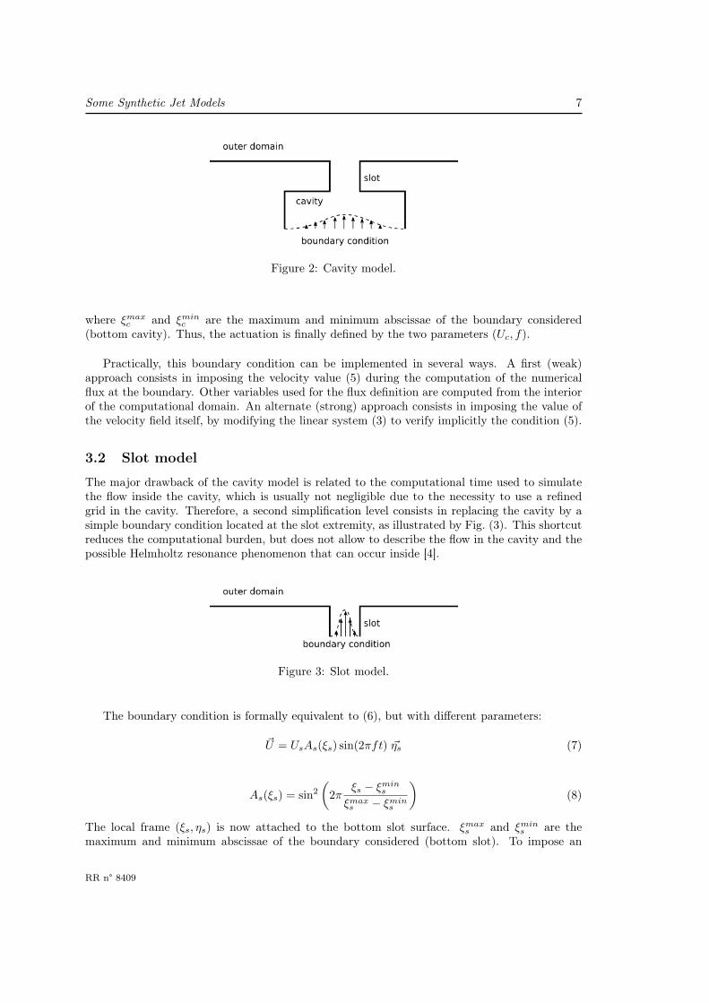
3.1 Cavity model

A first simplification consists in using a fixed computational domain. In that case, the move ofthe bottom surface of the cavity is modeled by imposing a prescribed boundary condition for theflow velocity [5] and possibly for the normal pressure gradient [15], as illustrated by Fig. (2).

In this study, we impose the value of the velocity at the bottom surface, as:

~U = UcAc(ξc) sin(2πft) ~ηc (5)

where Uc is the oscillation amplitude of the velocity at the cavity bottom surface, (ξc, ηc) a localframe system and f is the actuation frequency. Ac(ξc) describes the velocity profile along thesurface, which is here defined as:

Ac(ξc) = sin2

(2π

ξc − ξminc

ξmaxc − ξmin

c

)(6)

Inria


Figure 2: Cavity model.

where ξmaxc and ξmin

c are the maximum and minimum abscissae of the boundary considered(bottom cavity). Thus, the actuation is finally defined by the two parameters (Uc, f).

Practically, this boundary condition can be implemented in several ways. A first (weak)approach consists in imposing the velocity value (5) during the computation of the numericalflux at the boundary. Other variables used for the flux definition are computed from the interiorof the computational domain. An alternate (strong) approach consists in imposing the value ofthe velocity field itself, by modifying the linear system (3) to verify implicitly the condition (5).

3.2 Slot model

The major drawback of the cavity model is related to the computational time used to simulatethe flow inside the cavity, which is usually not negligible due to the necessity to use a refinedgrid in the cavity. Therefore, a second simplification level consists in replacing the cavity by asimple boundary condition located at the slot extremity, as illustrated by Fig. (3). This shortcutreduces the computational burden, but does not allow to describe the flow in the cavity and thepossible Helmholtz resonance phenomenon that can occur inside [4].

Figure 3: Slot model.

The boundary condition is formally equivalent to (6), but with different parameters:

~U = UsAs(ξs) sin(2πft) ~ηs (7)

As(ξs) = sin2

(2π

ξs − ξmins

ξmaxs − ξmin

s

)(8)

The local frame (ξs, ηs) is now attached to the bottom slot surface. ξmaxs and ξmin

s are themaximum and minimum abscissae of the boundary considered (bottom slot). To impose an

RR n° 8409


equivalent flow rate, the following relationship should be verified:

Us = Ucξmaxc − ξmin

c

ξmaxs − ξmin

s

(9)

The practical implementation of the boundary condition is exactly the same as the one used forthe cavity model.

3.3 Boundary condition model

Finally, the simplest model just consists in imposing a boundary condition for the velocity at theslot exit, as illustrated by Fig. (4). This model makes the grid generation process slightly easier,but the benefit is not significant, because the mesh should anyway account for the jet, as shownin the following numerical study. This model does not allow to describe the interaction betweenthe flow in the outer domain and the flow exiting the slot. However, this model is certainly themost used in the literature due to its implementation ease.

Figure 4: Boundary model.

In practice, the boundary condition is the same as previously, defined by (7-8).

4 Test-case descriptionTo compare the flows predicted by the different models and quantify the impact of the numericalparameters, we consider as test-case a single synthetic jet located on a flat plate and interactingwith a boundary layer, as illustrated by Fig. (5). The baseline case, without actuator, correspondsto the zero pressure gradient flat plate verification case proposed by NASA and fully defined athttp://turbmodels.larc.nasa.gov/flatplate.html. The plate length is 2 m, whereas thecomputational domain height is 30 cm. The distance between the inlet boundary and the plateis 40 cm, and the distance between the stagnation point and the jet center is 50.25 cm. The slotwidth measures h = 5 mm. The length of the slot is twice its width 2h. The cavity dimension is9h× h.

The reference flow conditions are the following :

ρref 1.363 kg/m3

uref 69.437 m/spref 115056 Paµref 1.9 10−5 Pa s

The resulting Mach and Reynolds numbers are respectively Mref = 0.2 and Reref = 5 106.Note that the resulting boundary layer thickness at the actuation location is about twice theslot width. A validation of the flow simulation without actuation is first achieved, in terms ofskin friction coefficient and velocity profile by comparing with experiments and other codes, as

Inria

http://turbmodels.larc.nasa.gov/flatplate.html


Figure 5: Test-case description.

Figure 6: Comparison of the friction coefficient along the plate (without actuation).

illustrated by Figs. (6-7) for the Spalart-Allmaras model.

All inlet / outlet boundary conditions are imposed weakly. At the inlet boundary, the veloc-ity value uref and density ρref are imposed, while the pressure is computed from the interiordomain. On the contrary, an imposed pressure condition of value pref is prescribed at the outletboundary. For the far-field condition, boundary values are computed thanks to Riemann invari-ants.

Two sets of actuation parameters are tested. The first one corresponds to a rather lowfrequency - low amplitude actuation, whereas the second one exhibits high frequency - high

RR n° 8409


Figure 7: Comparison of the velocity profiles at outlet (without actuation).

amplitude characteristics:

Actuation 1 f = 50 Hz Us = Uref/2 = 34.72 m/sActuation 2 f = 500 Hz Us = 2Uref = 138.87 m/s

For all the computations below, the time-step is chosen to account for 200 steps for each actu-ation period. Therefore, the time-step is defined as ∆t1 = 1. 10−4 s for the first actuation, and∆t2 = 1. 10−5 s for the second one. The unsteady simulations are initialized by the steady statesolutions corresponding to the flows without actuation. For each time-step, a stopping criterioncorresponding to a reduction of 3 orders of the non-linear residuals is adopted.

The baseline grids used for the three models are depicted on Figs. (5-11) and count Nc =36848, Ns = 19304 and Nb = 17424 vertices respectively, for the cavity model, the slot modeland the boundary model respectively. The maximal aspect ratio of the cells is about 40000. Thenumber of vertices located on the jet exit is 40. Note that the grids are identical in the outerdomain.

Figure 8: Global view of the mesh.

Inria


Figure 9: Mesh in the vicinity of the actuator, cavity model.

Figure 10: Mesh in the vicinity of the actuator, slot model.

Figure 11: Mesh in the vicinity of the actuator, boundary model.

RR n° 8409


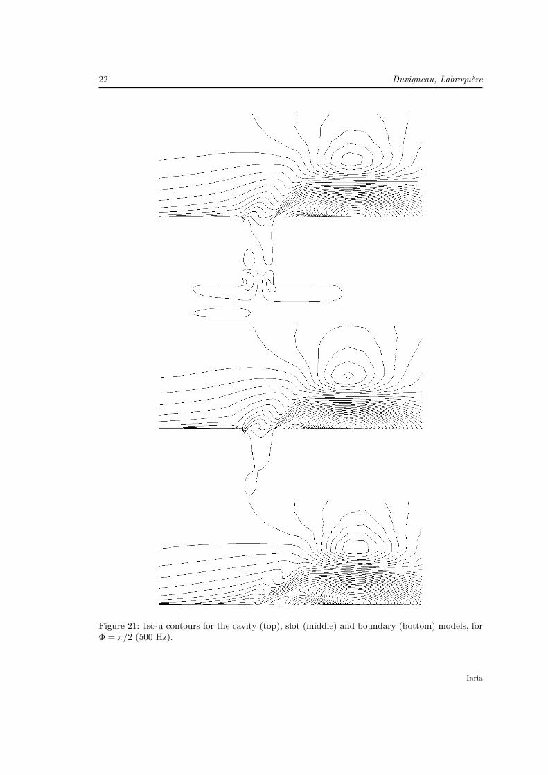
5 Comparison of the synthetic jet modelsComputations are carried out until a periodic flow is observed. Comparisons of the two velocitycomponents for the three models, in the vicinity of the actuator, are provided by Figs. (12-19)for the first actuation, and by Figs. (20-27) for the second actuation. On these figures, the phaseΦ = 0 corresponds to the maximum blowing time and Φ = π to the maximum suction time. TheSST k − ω turbulence closure is used here.

Clearly, the flows obtained using the three models are close to each other. The boundarymodel generates obviously a more symmetric flow at the slot exit, due to the boundary conditionon the velocity. The slot and the cavity models allow to compute the flow in the slot, which ischaracterized by strong asymmetry and generates a more intense flow at the slot corners. Onecan notice that the cavity and slot models only differ at the bottom part of the slot, with anegligible influence on the flow in the outer domain. The second actuation, with high frequencyand amplitude, exhibits larger discrepancies.

A comparison of the drag coefficient is also performed, as a more global assessment criterion.Fig. (28) confirms that the cavity and boundary models predict very similar flows, whereas theboundary model slightly underestimates the drag coefficient value, especially for the second ac-tuation parameters.

The conclusions of these comparisons are the following: although the cavity model is far moreCPU-demanding than the slot model, the discrepancy between the two predicted flows is weak,in terms of local field values and global drag coefficient. The boundary model predicts similarflows. However, some differences are reported for high-frequency high-amplitude actuation. Inthe perspective of more complex studies, the slot model seems to be the best compromise, interms of CPU cost and flow prediction. An alternate approach could be to capture the velocityprofile computed at the slot exit using the cavity model, and use it as boundary condition for theboundary model. However, if one considers a jet with varying parameters (amplitude, frequency,location), it is not clear that the selected profile will correspond to the new conditions. For thesereasons, the boundary model could be considered as reasonable for design optimization purpose,provided that actuation characteristics are moderate.

Inria


Figure 12: Iso-u contours for the cavity (top), slot (middle) and boundary (bottom) models, forΦ = 0 (50 Hz).

RR n° 8409


Figure 13: Iso-u contours for the cavity (top), slot (middle) and boundary (bottom) models, forΦ = π/2 (50 Hz).

Inria


Figure 14: Iso-u contours for the cavity (top), slot (middle) and boundary (bottom) models, forΦ = π (50 Hz).

RR n° 8409


Figure 15: Iso-u contours for the cavity (top), slot (middle) and boundary (bottom) models, forΦ = 3π/2 (50 Hz).

Inria


Figure 16: Iso-v contours for the cavity (top), slot (middle) and boundary (bottom) models, forΦ = 0 (50 Hz).

RR n° 8409


Figure 17: Iso-v contours for the cavity (top), slot (middle) and boundary (bottom) models, forΦ = π/2 (50 Hz).

Inria


Figure 18: Iso-v contours for the cavity (top), slot (middle) and boundary (bottom) models, forΦ = π (50 Hz).

RR n° 8409


Figure 19: Iso-v contours for the cavity (top), slot (middle) and boundary (bottom) models, forΦ = 3π/2 (50 Hz).

Inria


Figure 20: Iso-u contours for the cavity (top), slot (middle) and boundary (bottom) models, forΦ = 0 (500 Hz).

RR n° 8409


Figure 21: Iso-u contours for the cavity (top), slot (middle) and boundary (bottom) models, forΦ = π/2 (500 Hz).

Inria


Figure 22: Iso-u contours for the cavity (top), slot (middle) and boundary (bottom) models, forΦ = π (500 Hz).

RR n° 8409


Figure 23: Iso-u contours for the cavity (top), slot (middle) and boundary (bottom) models, forΦ = 3π/2 (500 Hz).

Inria


Figure 24: Iso-v contours for the cavity (top), slot (middle) and boundary (bottom) models, forΦ = 0 (500 Hz).

RR n° 8409


Figure 25: Iso-v contours for the cavity (top), slot (middle) and boundary (bottom) models, forΦ = π/2 (500 Hz).

Inria


Figure 26: Iso-v contours for the cavity (top), slot (middle) and boundary (bottom) models, forΦ = π (500 Hz).

RR n° 8409


Figure 27: Iso-v contours for the cavity (top), slot (middle) and boundary (bottom) models, forΦ = 3π/2 (500 Hz).

Inria


0.04 0.05 0.06 0.07 0.08time

0.0053

0.0054

0.0055

0.0056

0.0057

drag

coe

ffici

ent

CavitySlotBoundary

0.01 0.011 0.012 0.013 0.014time

0.0051

0.0052

0.0053

0.0054

0.0055

0.0056

0.0057

drag

coe

ffici

ent

CavitySlotBoundary

Figure 28: Time evolution of the drag coefficient, for the first actuation (top) and second actu-ation (bottom).

RR n° 8409


6 Impact of numerical parametersIn this section, we investigate the influence of some numerical parameters on the flow predicted.In the perspective of design optimization, we restrict this study to the boundary condition modelfor the actuation 1 and we use the drag coefficient as main comparison criterion. More precisely,we test the influence of the choice of the boundary condition type for the jet (weak vs. strong)and we measure the impact of the convergence criterion used for each time step. The SST k−ωturbulence closure is used here again.

0.04 0.05 0.06 0.07 0.08time

0.0053

0.0054

0.0055

0.0056

0.0057

drag

coe

ffici

ent

WeakStrong

Figure 29: Time evolution of the drag coefficient, for weak and strong boundary conditions.

0.04 0.05 0.06 0.07 0.08time

0.0053

0.0054

0.0055

0.0056

0.0057

drag

coe

ffici

ent

2 orders3 orders

Figure 30: Time evolution of the drag coefficient, for different non-linear convergence criteria.

The evolution of the drag coefficient computed using weak and strong boundary conditionsis depicted in Fig. (29). As seen, the discrepancy is not relevant. Indeed, the iterative process

Inria


carried out at each time-step makes the two approaches nearly identical.

Fig. (30) shows the same quantity, when different parameters are used as stopping criterionfor the non-linear iterative process. Here again, the discrepancy is small, which indicates thatthe flow at each time-step is well converged.

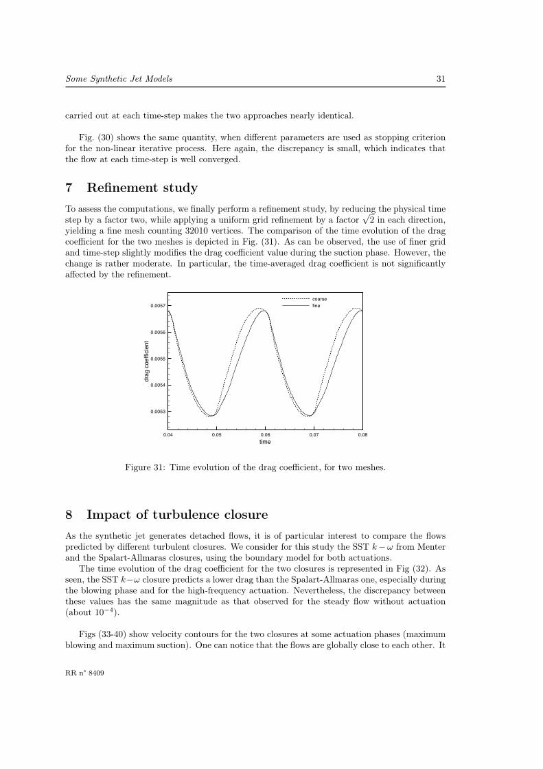
7 Refinement studyTo assess the computations, we finally perform a refinement study, by reducing the physical timestep by a factor two, while applying a uniform grid refinement by a factor

√2 in each direction,

yielding a fine mesh counting 32010 vertices. The comparison of the time evolution of the dragcoefficient for the two meshes is depicted in Fig. (31). As can be observed, the use of finer gridand time-step slightly modifies the drag coefficient value during the suction phase. However, thechange is rather moderate. In particular, the time-averaged drag coefficient is not significantlyaffected by the refinement.

0.04 0.05 0.06 0.07 0.08time

0.0053

0.0054

0.0055

0.0056

0.0057

drag

coe

ffici

ent

coarsefine

Figure 31: Time evolution of the drag coefficient, for two meshes.

8 Impact of turbulence closureAs the synthetic jet generates detached flows, it is of particular interest to compare the flowspredicted by different turbulent closures. We consider for this study the SST k−ω from Menterand the Spalart-Allmaras closures, using the boundary model for both actuations.

The time evolution of the drag coefficient for the two closures is represented in Fig (32). Asseen, the SST k−ω closure predicts a lower drag than the Spalart-Allmaras one, especially duringthe blowing phase and for the high-frequency actuation. Nevertheless, the discrepancy betweenthese values has the same magnitude as that observed for the steady flow without actuation(about 10−4).

Figs (33-40) show velocity contours for the two closures at some actuation phases (maximumblowing and maximum suction). One can notice that the flows are globally close to each other. It

RR n° 8409


0.04 0.05 0.06 0.07 0.08time

0.0053

0.0054

0.0055

0.0056

0.0057

drag

coe

ffici

ent

SST k-wSpalart-Allmaras

0.01 0.011 0.012 0.013 0.014time

0.0052

0.0053

0.0054

0.0055

drag

coe

ffici

ent

SST k-wSpalart-Allmaras

Figure 32: Time evolution of the drag coefficient for different turbulence closures, for the firstactuation (top) and second actuation (bottom).

is confirmed that they differ mainly during the blowing phase, the SST k− ω closure generatinga more vortical flow, with more intense gradients, than the Spalart-Allmaras one.

Inria


Figure 33: Iso-u contours for the SST k − ω (top) and Spalart-Allmaras (bottom) closures, forΦ = 0 (50 Hz).

Figure 34: Iso-u contours for the SST k − ω (top) and Spalart-Allmaras (bottom) closures, forΦ = π (50 Hz).

RR n° 8409


Figure 35: Iso-v contours for the SST k − ω (top) and Spalart-Allmaras (bottom) closures, forΦ = 0 (50 Hz).

Figure 36: Iso-v contours for the SST k − ω (top) and Spalart-Allmaras (bottom) closures, forΦ = π (50 Hz).

Inria


Figure 37: Iso-u contours for the SST k − ω (top) and Spalart-Allmaras (bottom) closures, forΦ = 0 (500 Hz).

Figure 38: Iso-u contours for the SST k − ω (top) and Spalart-Allmaras (bottom) closures, forΦ = π (500 Hz).

RR n° 8409


Figure 39: Iso-v contours for the SST k − ω (top) and Spalart-Allmaras (bottom) closures, forΦ = 0 (500 Hz).

Figure 40: Iso-v contours for the SST k − ω (top) and Spalart-Allmaras (bottom) closures, forΦ = π (500 Hz).

Inria


9 ConclusionThe objective of the current study was to simulate a synthetic jet in a turbulent boundary layerflow, compare the flows predicted by some actuator models and assess the turbulence closures inthis context. This study can be considered as a preparatory work before optimization of controlparameters for more complex problems.

It has been found that the actuator model including the slot description is a satisfactorycompromise between the complexity of including the whole cavity and the simplicity of usingonly a boundary condition. The numerical parameters (convergence criterion, grid size, timestep, type of boundary condition) have been set to reasonable values for the problem considered.

Regarding the influence of turbulence closures, a moderate discrepancy between the Spalart-Allmaras and the SST k − ω closures has been reported, the latter generating a more intenseflow at blowing. However, it would be interesting to consider more different models for futurestudies, such as non-linear algebraic stress models.

AcknowlegementThis study is supported by the 7th Framework Program of the European Union, project number266326 "MARS".

RR n° 8409


References

[1] P. Batten, N. Clarke, C. Lambert, and M. Causon. On the choice of wavespeeds for the hllcRiemann solver. SIAM J. Sci. Comput., 18(6):1553–1570, November 1997.

[2] M. Bergmann and L. Cordier. Optimal control of the cylinder wake in the laminar regimeby trust-region methods and pod reduced-order models. J. Comput. Physics, 227(16), 2008.

[3] A. Carnarius, F. Thiele, E. Oezkaya, A. Nemili, and N. Gauger. Optimization of active flowcontrol of a naca 0012 airfoil by using a continuous adjoint approach. In European Congresson Computational Methods in Applied Sciences and Engineering, Vienna, Austria, 2012.

[4] J. Dandois. Contrôle des décollements par jet synthétique. PhD thesis, University Paris VI,2007.

[5] J. Dandois, E. Garnier, and P. Sagaut. Unsteady simulation of synthetic jet in a crossflow.AIAA Journal, 44(2), 2006.

[6] A. Dervieux and J.-A. Désidéri. Compressible flow solvers using unstructured grids. INRIAResearch Report 1732, June 1992.

[7] J.F. Donovan, L.D. Kral, and A.W. Cary. Active flow control applied to an airfoil. AIAAPaper 98–0210, January 1998.

[8] R. Duvigneau, A. Hay, and M. Visonneau. Optimal location of a synthetic jet on an airfoilfor stall control. Journal of Fluid Engineering, 129(7):825–833, July 2007.

[9] R. Duvigneau and M. Visonneau. Optimization of a synthetic jet actuator for aerodynamicstall control. Computers and Fluids, 35:624–638, July 2006.

[10] R. P. Dwight. Efficiency improvements of RANS-based analysis and optimization usingimplicit and adjoint methods on unstructured grids. PhD thesis, University of Manchester,2006.

[11] J.A. Ekaterinaris. Active flow control of wing separated flow. ASME FEDSM’03 Joint FluidsEngineering Conference, Honolulu, Hawai, USA, July 6-10, 2003.

[12] J.L. Gilarranz, L.W. Traub, and O.K. Rediniotis. Characterization of a compact, high powersynthetic jet actuator for flow separation control. AIAA Paper 2002–0127, September 2002.

[13] J. W. He, R. Glowinski, R. Metcalfe, A. Nordlander, and J. Periaux. Active control anddrag optimization for flow past a circular cylinder: I. oscillatory cylinder rotation. Journalof Computational Physics, 163(1):83 – 117, 2000.

[14] T. Kloczko, C. Corre, and A. Beccantini. Low-cost implicit schemes for all-speed flows onunstructured meshes. International Journal for Numerical Methods in Fluids, 58(5):493–526,October 2008.

[15] L.D. Kral, J.F. Donovan, A.B. Cain, and A.W. Cary. Numerical simulation of synthetic jetactuators. In AIAA Paper 97-1824, 1997.

[16] F.R. Menter. Two-equation eddy-viscosity turbulence models for engineering applications.AIAA Journal, 32(8), 1994.

Inria


[17] A. Seifert, A. Darabi, and I. Wygnanski. Delay of airfoil stall by periodic excitation. AIAAJournal, 33(4):691–707, July 1996.

[18] B. Smith and A. Glezer. Vectoring and small-scale motions effected in free shear flows usingsynthetic jet actuators. In AIAA Paper 97-0213, 1997.

[19] A. Zymaris, D. Papadimitriou, K. Giannakoglou, and C. Othmer. Optimal location fosuction or blowing jets using the continuous adjoint approach. In European Congress onComputational Methods in Applied Sciences and Engineering ECCOMAS 2010 Lisbon, 2010.

RR n° 8409


Contents1 Introduction 3

2 Numerical framework 42.1 Discretization . . . . . . . . . . . . . . . . . . . . . . . . . . . . . . . . . . . . . . 42.2 Turbulence closures . . . . . . . . . . . . . . . . . . . . . . . . . . . . . . . . . . . 5

3 Synthetic jet models 53.1 Cavity model . . . . . . . . . . . . . . . . . . . . . . . . . . . . . . . . . . . . . . 63.2 Slot model . . . . . . . . . . . . . . . . . . . . . . . . . . . . . . . . . . . . . . . . 73.3 Boundary condition model . . . . . . . . . . . . . . . . . . . . . . . . . . . . . . . 8

4 Test-case description 8

5 Comparison of the synthetic jet models 12

6 Impact of numerical parameters 30

7 Refinement study 31

8 Impact of turbulence closure 31

9 Conclusion 37

Inria

RESEARCH CENTRESOPHIA ANTIPOLIS – MÉDITERRANÉE

2004 route des Lucioles - BP 9306902 Sophia Antipolis Cedex

PublisherInriaDomaine de Voluceau - RocquencourtBP 105 - 78153 Le Chesnay Cedexinria.fr

ISSN 0249-6399

comparison and assessment of some synthetic jet models

Documents