NBER WORKING PAPER SERIES

COMMODITY MARKET DISINTEGRATION IN THE INTERWAR PERIOD

William HynesDavid S. Jacks

Kevin H. O'Rourke

Working Paper 14767http://www.nber.org/papers/w14767

NATIONAL BUREAU OF ECONOMIC RESEARCH1050 Massachusetts Avenue

Cambridge, MA 02138March 2009

Work on this paper commenced while O'Rourke was a Government of Ireland Senior Research Fellow,and he thanks the Irish Research Council for the Humanities and Social Sciences for their generousfinancial support. Jacks gratefully acknowledges the Social Sciences and Humanities Research Councilof Canada for research support. The views expressed herein are those of the author(s) and do not necessarilyreflect the views of the National Bureau of Economic Research.

NBER working papers are circulated for discussion and comment purposes. They have not been peer-reviewed or been subject to the review by the NBER Board of Directors that accompanies officialNBER publications.

© 2009 by William Hynes, David S. Jacks, and Kevin H. O'Rourke. All rights reserved. Short sectionsof text, not to exceed two paragraphs, may be quoted without explicit permission provided that fullcredit, including © notice, is given to the source.

Commodity Market Disintegration in the Interwar Period William Hynes, David S. Jacks, and Kevin H. O'Rourke NBER Working Paper No. 14767 March 2009 JEL No. F13,F15,F59,N70

ABSTRACT

Using data collected by the International Institute of Agriculture, we document the disintegration of international commodity markets between 1913 and 1938. There was dramatic disintegration during World War I, gradual reintegration during the 1920s, and then a very substantial disintegration after 1929. The period saw the unravelling of a great many of the integration gains of the 1870-1913 period. While increased transport costs certainly help to explain the wartime disintegration, they cannot explain the post-1929 increase in trade costs. Protectionism seems the most likely alternative candidate.

William Hynes Kevin H. O'Rourke Wadham College Department of Economics and IIIS Parks Road Trinity College Oxford Dublin 2, IRELAND OX1 3PN and NBER United Kingdom kevin.orourke@tcd.ie william.hynes@wadh.ox.ac.uk

David S. Jacks Department of Economics Simon Fraser University 8888 University Drive Burnaby, BC V5A 1S6 CANADA and NBER dsjacks@gmail.com

1. Introduction

Since the early work of pioneers such as Jeffrey Williamson (1974), Knick Harley

(1978, 1980), John Hurd (1975) or Jacob Metzer (1974) there has been an explosion of work

documenting the integration of national and international commodity markets during the 19th

century. Successive papers have advanced the state of our knowledge along several

dimensions. A small minority (e.g. O'Rourke and Williamson 1994, Klovland 2005) have

documented patterns of price convergence or divergence for commodities other than the

grains which have been the focus of most papers. Some authors, notably Karl Gunnar

Persson (e.g. Persson 2004), have demonstrated the importance of comparing commodities of

identical qualities in different markets. And during the past decade or so, much more

sophisticated econometric procedures have been used to identify both the speed with which

commodity prices moved back to equilibrium after a shock, and the trade costs which

determined whether such an adjustment process would take place in the first place (e.g.

Ejrnaes and Persson 2000).

Recent work has broadened the scope of these investigations well beyond the late

19th century. David Jacks (2005, 2006) and Federico and Persson (2007) have established

that international commodity markets were becoming better integrated throughout the post­

1815 period, and not just after 1870. O'Rourke and Williamson (2002) find no evidence of

commodity market integration between continents before 1800, while the evidence provided

by Jacks (2004) and Özmucur and Pamuk (2007) for market integration within early modern

Europe is decidedly mixed. Meanwhile, international economists have recently started to

uncover evidence of international price convergence for a variety of consumer goods during

the late 20th century, although this finding is at odds with what little we know about

international agricultural markets during the same period (Engel and Rogers 2004, Goldberg

and Verboven 2005, Parsley and Wei 2002, O’Rourke 2002, Federico and Persson 2007).

2

Strikingly, however, there has been little or no work documenting price convergence

or divergence during the interwar period. This is surprising, since the years after 1929 saw a

collapse in world trade which has been extensively studied, as well as a rise in protectionism

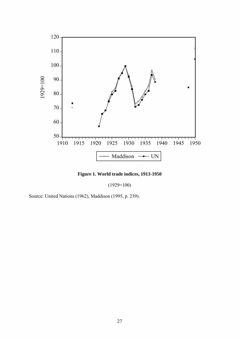
which has also been the subject of much scholarly attention. One of the classic questions

which many have asked regarding the period is: can this post-1929 collapse in world trade

(documented in Figure 1) be attributed to the Smoot-Hawley tariff of 1930 in the United

States, and equivalent import restrictions imposed elsewhere, or was it simply a reflection of

declining world output? Somewhat embarrassingly for economists to whom policies such as

Smoot-Hawley symbolise the folly of interwar economic policy-making, quantitative

analyses of the episode have tended to downplay the role of tariffs in explaining the world

trade slump, emphasising instead the role of falling demand and output (Irwin 1998).

However, Jacob Madsen (2001) argues that discretionary increases in protection were as

important as nominal income declines in explaining the post-1929 world trade slump.

Presumably, if trade barriers had contributed to the fall of world trade, then this would

have manifested itself in an increase in price gaps between markets, leading (ceteris paribus)

to an increase in import prices, a decline in export prices, and a decline in trade volumes, with

the size of all three effects depending upon elasticities of supply and demand. Increasing

price gaps is a necessary, if not sufficient, condition for protectionism to have had any effects

on world trade whatsoever. It thus seems as though the question of what happened to interwar

commodity market integration should be of interest not just to scholars of market integration

per se, but to those interested in the international economy of the period more generally. And

yet, very little work has been done on the subject to date. One exception is Federico and

Persson (2007), who look at world wheat markets over the past two centuries and find (using

annual data) that while these were extremely well integrated in the early 1920s, there was a

sharp increase in international price variance in the years after 1929. The aim of this paper is

3

to provide more such evidence, using higher-frequency data and more sophisticated

techniques, for a greater range of commodities, and to ask: what was the impact of World

War I on international commodity markets? To what extent did these recover during the

1920s? Did the years after 1929 see a further disintegration of international commodity

markets, and if so, was this disintegration severe enough to leave these markets less well

integrated than they had been before 1914? And what were the causes of the disintegration?

Was it due to rising transportation costs, as suggested by Estevadeordal, Frantz and Taylor

(2003), or to policy, or to some combination of the two?

2. Empirics

Data

The primary source for this study is the International Institute of Agriculture’s

International Yearbook of Agricultural Statistics. Although this publication provides a wealth

of information on international commodity markets during the interwar period, it has not yet

been exploited by economic historians, as far as we know. The Institute was founded in 1905

and headquartered in Rome. The IIA was a “world clearinghouse for data on crops, prices,

and trade to protect the common interests of farmers of all nations.” Thus, it was the first

international organization dedicated to the task of generating and publicizing world

agricultural data. Initially comprising forty nations, membership was extended to 51 by 1913.

It was succeeded in 1945 by the United Nation’s Food and Agricultural Organization (FAO).

The first statistical Yearbook was produced in 1909 and covered a wide range of

statistical material, from land area and population to agricultural production and agricultural

prices. After World War I, these volumes were published in subsequent years from 1920 to

1939. Their express purpose was to document the changes in global commodity markets after

the First World War. To quote, “the opinion was widely held that world economy [sic] would

4

return to the position existing on the eve of the conflagration so that data for the years

immediately preceding the War could be taken in a sense to represent the normal and thus to

constitute a good basis of comparison” (International Institute of Agriculture, 1933).

The data collection efforts of the International Institute of Agriculture were

prodigious. They cover 374 weekly commodity price series over 46 commodity

classifications in locales as far-flung as Rangoon, Rio de Janeiro, and almost all conceivable

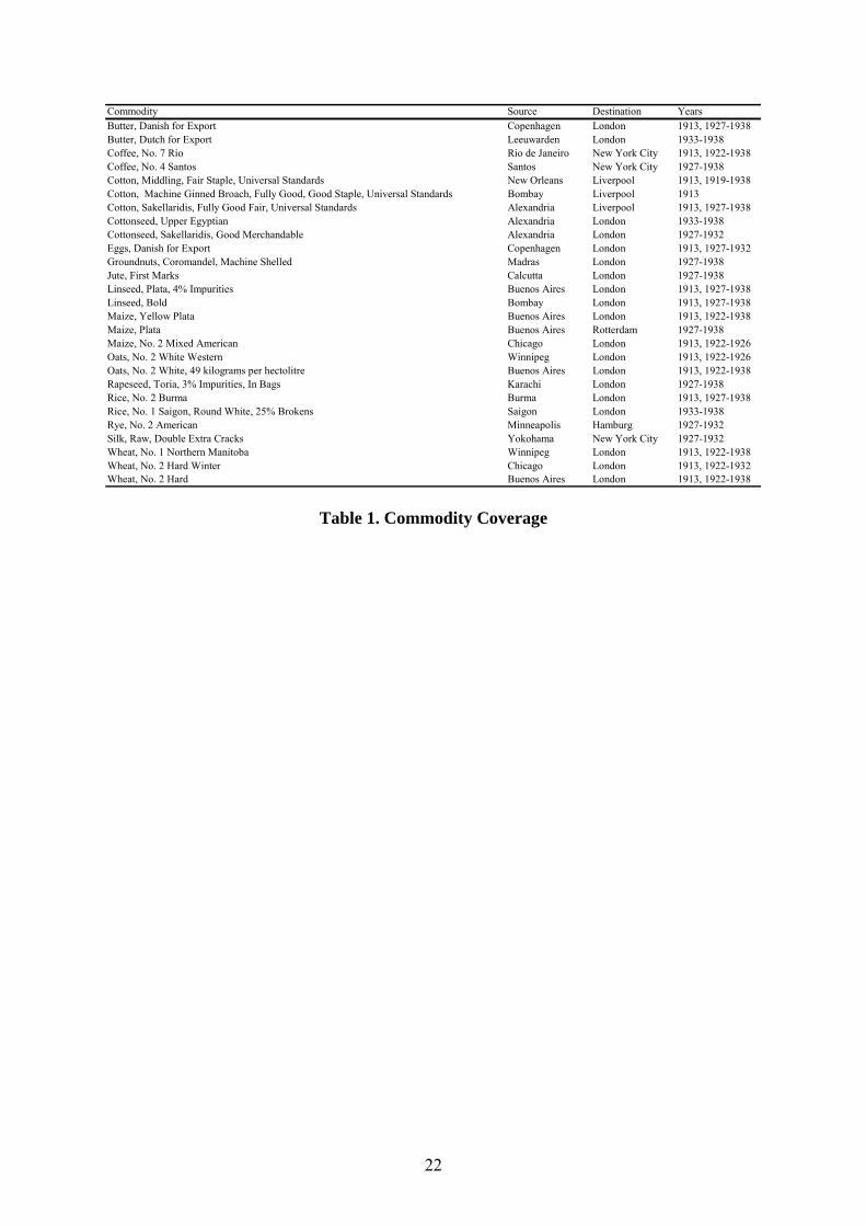
commercial ports in between. Of the 374 series, we are able to exactly match 27 commodity-

specific city pairs. These range from (Danish, creamery for export) butter in Copenhagen and

London to (No. 2 winter, American) wheat in Chicago and Liverpool. The commodity and

temporal coverage of our exact matches is documented in Table 1. We note that the

International Yearbook of Agricultural Statistics potentially allows for an even larger number

of matches. However, we have employed a very conservative selection criterion to ensure

that differences in product quality can play no role in our results.

In the International Yearbook of Agricultural Statistics, all weekly prices were quoted

in local currencies and measurements. Quoted prices in the source country were converted

into the currency and measurement of the matched destination country. For instance, (Danish,

creamery for export) butter in Copenhagen was quoted in crowns per 100 kilograms and

converted into shillings per hundredweight based on standard physical conversion rates and

nominal exchange rates derived from the Global Financial Database.

Methodology

Our chief focus is on estimating trade costs—that is, the costs of physically

transporting goods across markets inclusive of freight rates, tariffs and non-tariff barriers to

trade—over the interwar period, with an especial regard to comparing these to conditions

prevailing on the eve of the First World War. In recent years, a voluminous literature has

5

emerged in economics and economic history on how to gauge the trade costs separating

markets on the basis of price differentials (Balke and Fomby 1997; Obstfeld and Taylor

1997). For instance, Jacks (2005, 2006) documents the process of market integration in the

context of the Atlantic economy by examining grain price data from over 100 markets in

Europe and North America from 1800 to 1913.

In contrast to earlier work which looked mainly at average annual price gaps between

markets, the modern literature has relied on methods directly based on or indirectly inspired

by the threshold autoregression approach first developed by Tsay (1989). Here, we adopt the

latter approach and make use of an extremely parsimonious model of commodity market

integration. The basic idea is that agents—given the prevailing costs of transport, tariffs and

non-tariff barriers to trade, the costs of obtaining credit and contracting in foreign exchange

markets, etc.—will exploit all profitable opportunities in terms of price differentials. In this

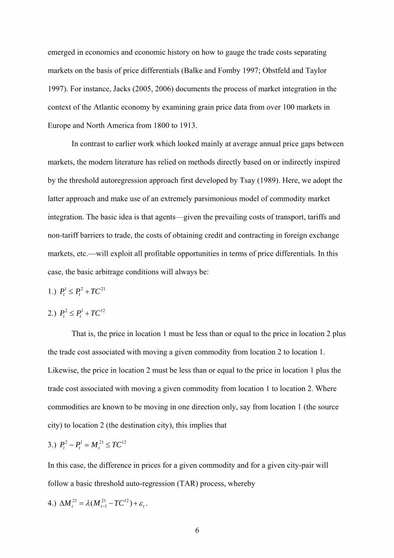
case, the basic arbitrage conditions will always be:

1 2 21 1.) Pt Pt TC

2 1 12 2.) Pt Pt TC

That is, the price in location 1 must be less than or equal to the price in location 2 plus

the trade cost associated with moving a given commodity from location 2 to location 1.

Likewise, the price in location 2 must be less than or equal to the price in location 1 plus the

trade cost associated with moving a given commodity from location 1 to location 2. Where

commodities are known to be moving in one direction only, say from location 1 (the source

city) to location 2 (the destination city), this implies that

2 1 21 123.) P P M TC t t t

In this case, the difference in prices for a given commodity and for a given city-pair will

follow a basic threshold auto-regression (TAR) process, whereby

21 21 124.) M (M TC ) .t t1 t

6

21In models of this class, λ is allowed to vary according to whether Mt1 is below (that is,

21 12 21 12 M TC ) or above (that is, M TC ) the threshold defined by the trade cost term, t1 t1

21 12TC12 . If M TC , then there are no profitable arbitrage opportunities available and λ ist1

21 12equal to zero. However, if M TC , then a profitable arbitrage opportunity exists, and we t1

assume that agents exploit such opportunities, which would imply that λ is negative.

The International Yearbook of Agricultural Statistics reports weekly observations on

commodity prices. Consequently, we are able to estimate TARs for every individual year

available. This comes at the cost of assuming a constant trade cost term for each year. Given

the slowly evolving dynamics of international shipping and commercial policy, this does not

seem to be too heroic an assumption. Finally, we are not open to the identification problem

highlighted by Coleman (2007). Given that the IIA reports exact commodity-specific city-

pair matches (for example, Danish creamery butter for export, in Copenhagen and London)

chosen to represent bilateral trading relations, the goods are traded between our city pairs by

definition, so there is little need to worry about the emergence of triangular arbitrage

shipments, which apparently characterised the pre-World War I gold trade between New

York City and London.

Results

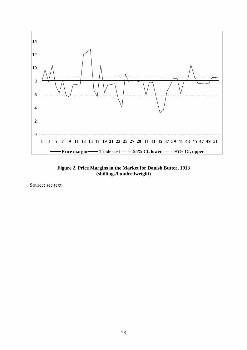
Figure 2 illustrates the estimation procedure for a single commodity for a given city-

pair in a given year. Here, we consider the case of the market for Danish butter for export in

Copenhagen and London in 1913. Throughout the year, the price in shillings per

hundredweight is always higher in London than in Copenhagen. Thus, the margin informs us

about the likely size of the composite trade costs—that is, all the costs of transportation and

transaction involved in exporting Danish creamery butter from Copenhagen to London.

7

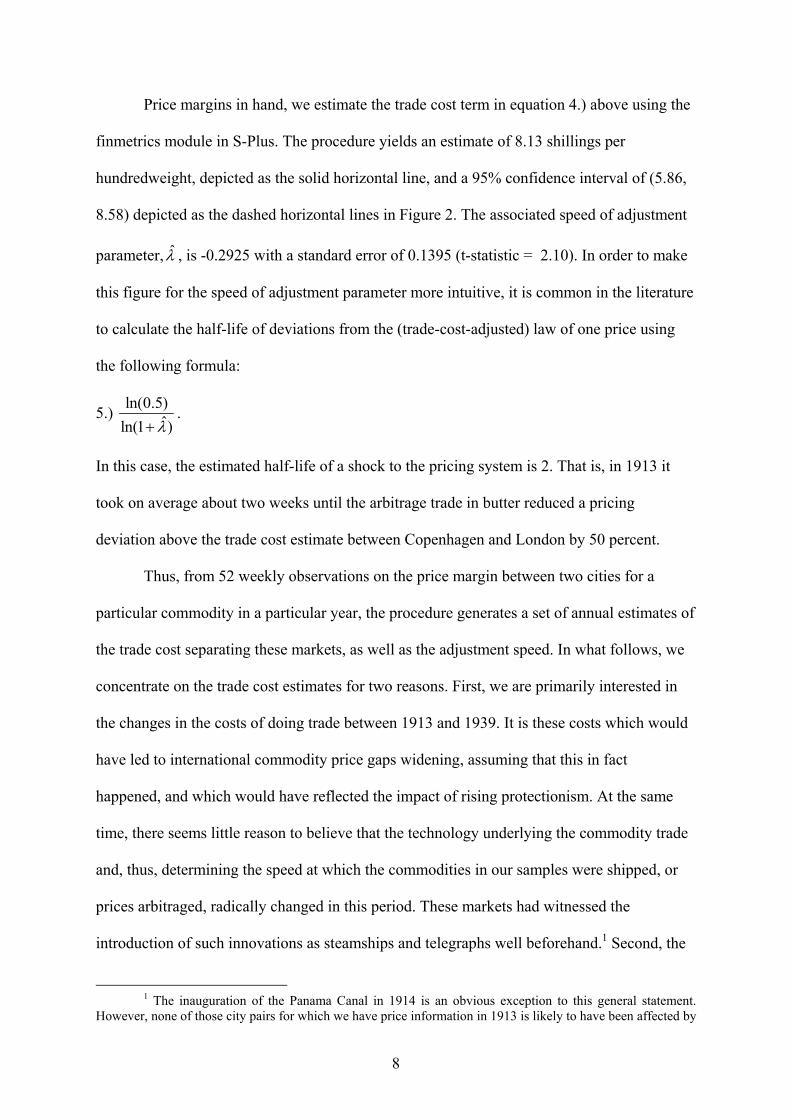
Price margins in hand, we estimate the trade cost term in equation 4.) above using the

finmetrics module in S-Plus. The procedure yields an estimate of 8.13 shillings per

hundredweight, depicted as the solid horizontal line, and a 95% confidence interval of (5.86,

8.58) depicted as the dashed horizontal lines in Figure 2. The associated speed of adjustment

parameter, ̂ , is -0.2925 with a standard error of 0.1395 (t-statistic = 2.10). In order to make

this figure for the speed of adjustment parameter more intuitive, it is common in the literature

to calculate the half-life of deviations from the (trade-cost-adjusted) law of one price using

the following formula:

ln(0.5) 5.) .

ln(1 ̂)

In this case, the estimated half-life of a shock to the pricing system is 2. That is, in 1913 it

took on average about two weeks until the arbitrage trade in butter reduced a pricing

deviation above the trade cost estimate between Copenhagen and London by 50 percent.

Thus, from 52 weekly observations on the price margin between two cities for a

particular commodity in a particular year, the procedure generates a set of annual estimates of

the trade cost separating these markets, as well as the adjustment speed. In what follows, we

concentrate on the trade cost estimates for two reasons. First, we are primarily interested in

the changes in the costs of doing trade between 1913 and 1939. It is these costs which would

have led to international commodity price gaps widening, assuming that this in fact

happened, and which would have reflected the impact of rising protectionism. At the same

time, there seems little reason to believe that the technology underlying the commodity trade

and, thus, determining the speed at which the commodities in our samples were shipped, or

prices arbitraged, radically changed in this period. These markets had witnessed the

introduction of such innovations as steamships and telegraphs well beforehand.1 Second, the

1 The inauguration of the Panama Canal in 1914 is an obvious exception to this general statement. However, none of those city pairs for which we have price information in 1913 is likely to have been affected by

8

identification of the threshold parameter comes off the entire set of observations for a given

year (generally 52), while the identification of the adjustment parameter comes off the subset

of observations that the TAR routine determines to be most likely to be above the trade-cost

threshold, resulting in less precision.2

In any case, most of the estimated coefficients are significant at the 10 percent level,

and, as predicted, we always find a negative adjustment parameter and a positive trade cost

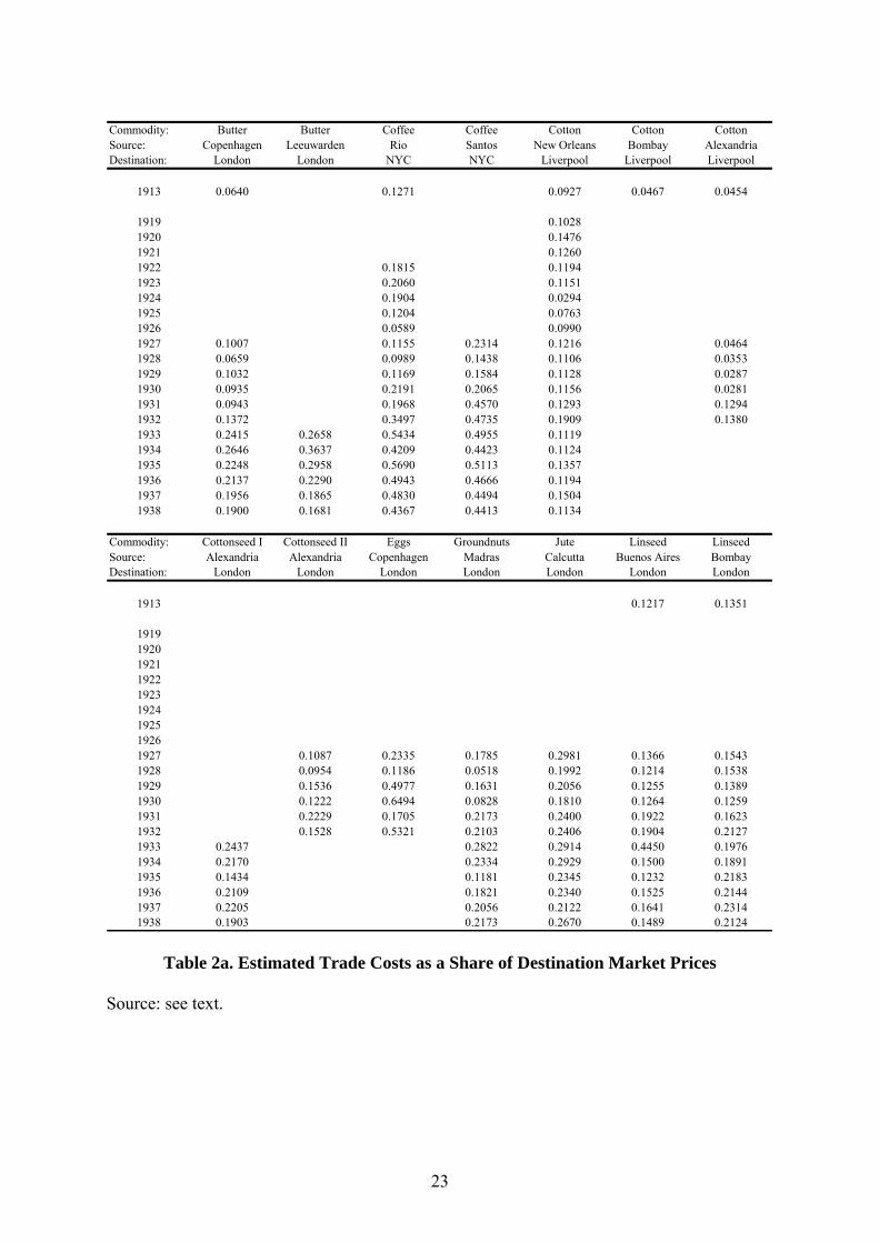
TC. We combine these commodity-, city pair-, year-specific estimates of trade costs with

information on the average annual prices of the same commodities in destination cities to

arrive at a unit-less measure of trade costs which is comparable across commodities and

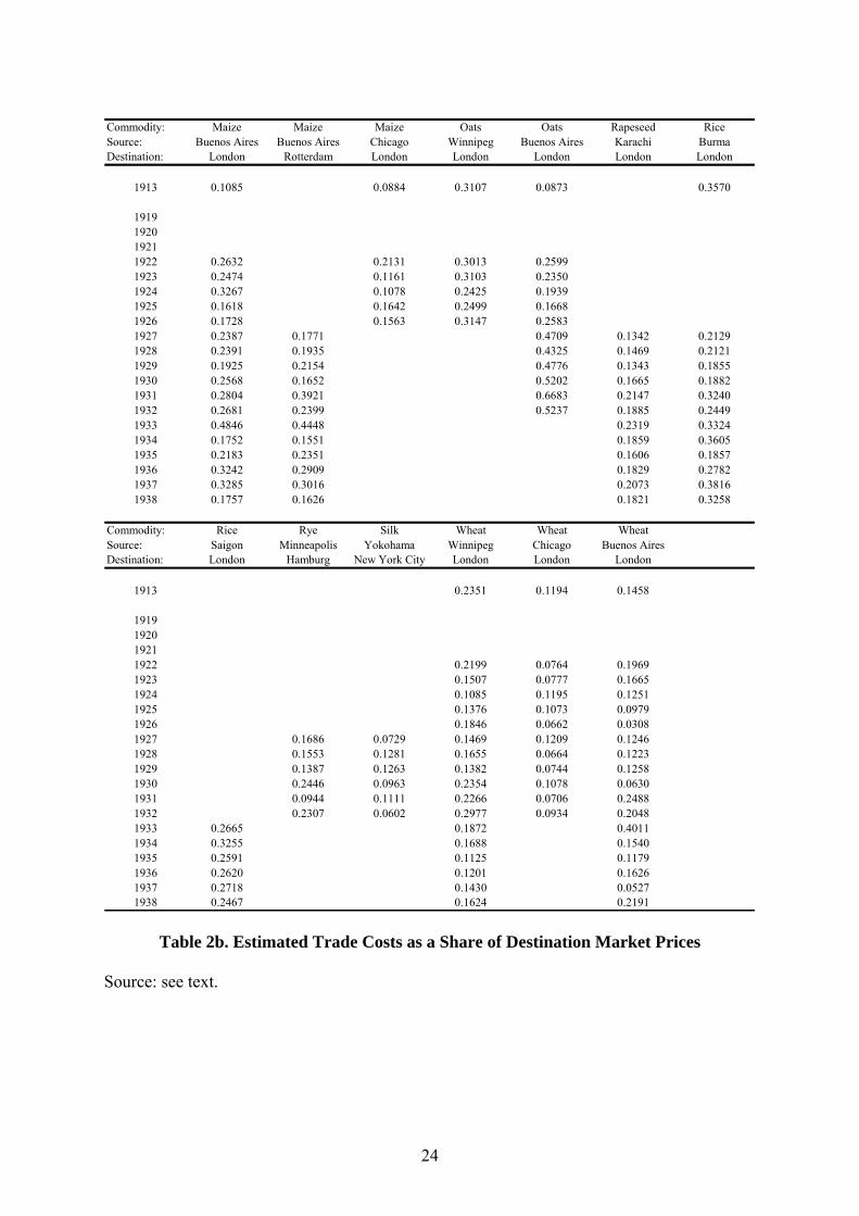
years. Tables 2a and 2b summarize the estimated trade costs as a share of destination market

prices for the 291 observations at our disposal.

The first finding which we want to discuss is the comparison between trade cost levels

in 1913 versus the post-war period. For the fourteen trade cost series at our disposal with

observations both in 1913 and in the post-war period, fully ten register an increase in trade

costs as a share of destination market prices. Regarding the four which register a decrease, we

note that three of these involved the trade in grains between North American and the United

Kingdom (oats between Winnipeg and London, wheat between Winnipeg and London, and

wheat between Chicago and London). These three exceptions are less surprising if we

consider the staggering heights of commercial activity in these trades—and presumably,

investment in the attendant handling and shipping facilities—achieved during World War I

(Food Research Institute, various years). Comparing trade costs in 1913 to those in 1922 for

those series with available data suggests that, on average, trade costs rose by 60%. The

its completion, as a quick review of Table 1 will confirm. We discuss interwar transportation technologies further below.

2 In an exercise to follow, we estimate two TARs on all pre-1930 observations, and all post-1929 observations, for the handful of commodities with sufficient data. These results bear out our expectation that adjustment speeds cannot be distinguished from one another, pre- and post-1929, but that estimates of trade costs can.

9

respective figures for 1927 and 1929 are 48% and 42%, suggesting that the international

economy was slowly converging back to the levels of integration set in 1913. The evidence

from the price data is thus consistent with the recovery in world trade volumes during the

1920s apparent in Figure 1.

The cataclysm of the Great Depression and the corresponding fallout in commercial

policy changed all of this. The ratio of trade costs in 1933 to trade costs in 1913 is a

staggering 2.59—that is, trade costs as a share of destination market prices had increased by

almost 160%. Furthermore, apart from some fits and starts in re-establishing some semblance

of order to international markets, the ratio still stood at 2.68 in 1938.

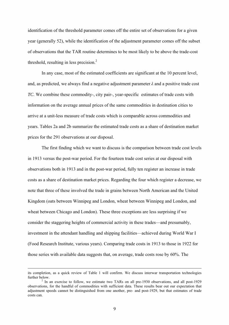
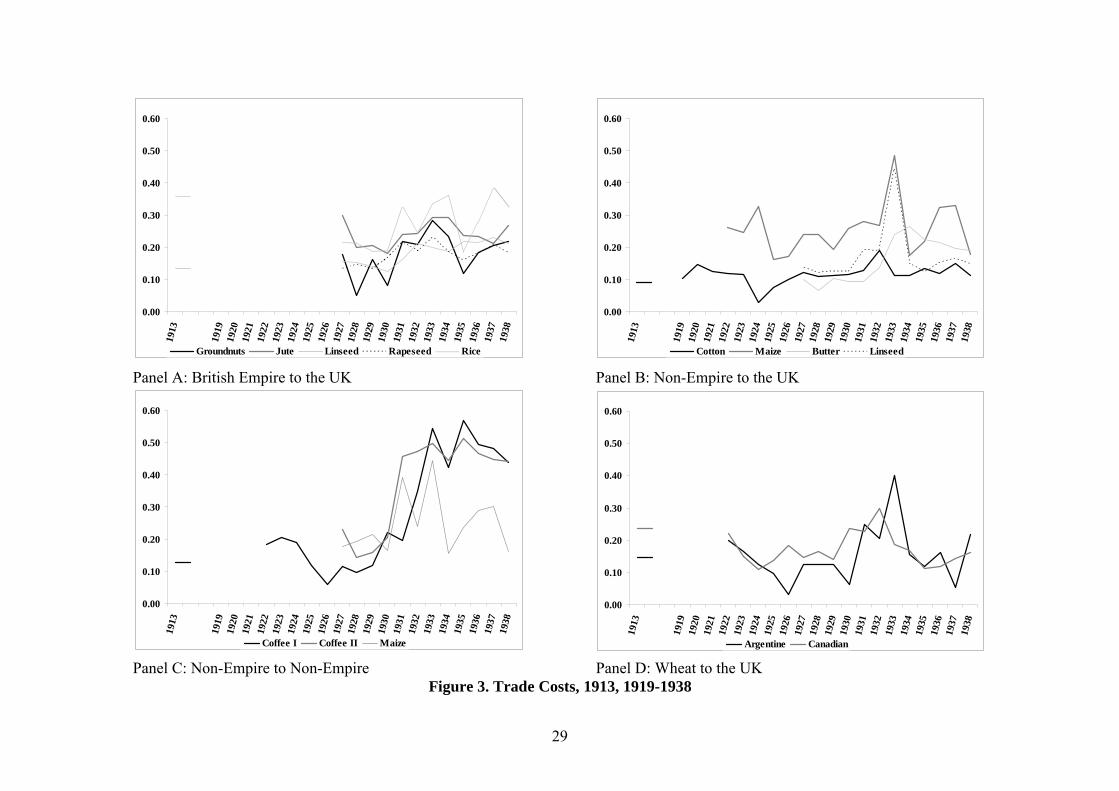
Some of these patterns can be detected in Figure 3. Rather than plot all the available

series, we simply consider those trade cost series which bridge the critical period from 1929

to 1933. That is, we are able to track individual commodity trade costs from the onset of the

Great Depression to the nadir in global trade and beyond. The figure distinguishes between

series representing different orientations of trade flows. Thus, in panel A there are five trade

cost series—groundnuts from Madras to London, jute from Calcutta to London, linseed from

Bombay to London, rapeseed from Karachi to London, and rice from Burma to London—

which represent trade between the British Empire (or, more precisely, British India including

Burma) and the United Kingdom. In panel B, there are four trade cost series—cotton from

New Orleans to Liverpool, maize from Buenos Aires to London, butter from Copenhagen to

London, and linseed from Buenos Aires to London—which represent trade between non-

British Empire countries and the United Kingdom. In panel C, there are three trade cost

series—coffee (I) from Rio de Janeiro to New York City, coffee (II) from Santos to New

York City, and maize from Buenos Aires to Rotterdam—which represent trade among non-

British Empire countries. Finally, in panel D, there are two trade cost series from Buenos

10

Aires and Winnipeg to London, which allow us to compare the trade in wheat to the United

Kingdom from British Empire and non-British Empire countries.

Across all panels, the series again demonstrate that trade costs were on the decline

during the 1920s. There appears to have been some retrenchment in the later 1920s, but this

seems more to be a slowing in the trend than a turning point. However, 1930 witnessed a

marked transition in the trade cost series. The average for all series shot up from 0.1511 in

1929 to 0.3350 in 1933. Of the fourteen series depicted in 1933, only one — cotton from

New Orleans to Liverpool — stood at a level comparable to that of 1929 (0.1119 versus

0.1128, respectively). And even in this case, cotton trade costs increased by 70% between

1929 and 1932. The series are also roughly synchronized on the downside with most

bottoming out no later than 1935. Finally, after stabilizing at levels generally higher than in

the 1920s, the averages show no clear trend in the years immediately preceding the outbreak

of World War II.

Even more telling than these generalized trends is the differences between Empire and

non-Empire trade. For the series in Panel A, involving trade between British Empire

countries and the United Kingdom, trade costs increased on average by 62% between 1929

and 1933. For the series in Panel B, involving trade between non-British Empire countries

and the United Kingdom, trade costs increased on average by 135% between 1929 and 1933,

or almost twice as much. Among the series in Panel C, involving trade among non-British

Empire countries, trade costs increased on average by 205%. Of course, the commodity

composition of trade flows differed across these three categories, and this matters since

commercial policy responses across goods and countries is likely to have been highly

asymmetric. It is therefore instructive to turn to the series in Panel D, showing trade costs for

wheat between Argentina and the United Kingdom on the one hand, and between Canada and

the United Kingdom on the other. Again, membership in the British Empire seems to have

11

mattered: Argentine trade costs increased by 219% between 1929 and 1933, while Canadian

trade costs increased by 35% over the same period. These patterns are consistent with the re­

orientation of world trade in light of the system of imperial preferences instituted in the

Import Duties Act and the Ottawa Conference of 1932 (Eichengreen and Irwin, 1995).

A longer run perspective: international price gaps, 1870-1938

Some authors, such as Giovanni Federico (2008), prefer to use simpler indicators,

such as the average annual price gaps between markets, as a measure of international

commodity market integration. In this section we therefore provide this evidence for the

interwar period, and compare interwar price gaps with those pertaining in the late 19th

century, so as to gain a longer-run perspective on interwar disintegration.

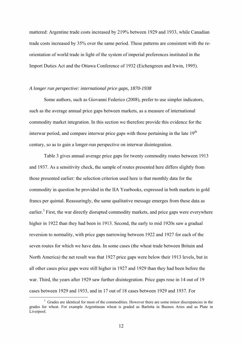
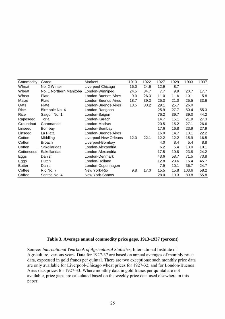
Table 3 gives annual average price gaps for twenty commodity routes between 1913

and 1937. As a sensitivity check, the sample of routes presented here differs slightly from

those presented earlier: the selection criterion used here is that monthly data for the

commodity in question be provided in the IIA Yearbooks, expressed in both markets in gold

francs per quintal. Reassuringly, the same qualitative message emerges from these data as

earlier.3 First, the war directly disrupted commodity markets, and price gaps were everywhere

higher in 1922 than they had been in 1913. Second, the early to mid 1920s saw a gradual

reversion to normality, with price gaps narrowing between 1922 and 1927 for each of the

seven routes for which we have data. In some cases (the wheat trade between Britain and

North America) the net result was that 1927 price gaps were below their 1913 levels, but in

all other cases price gaps were still higher in 1927 and 1929 than they had been before the

war. Third, the years after 1929 saw further disintegration. Price gaps rose in 14 out of 19

cases between 1929 and 1933, and in 17 out of 18 cases between 1929 and 1937. For

3 Grades are identical for most of the commodities. However there are some minor discrepancies in the grades for wheat. For example Argentinean wheat is graded as Barletta in Buenos Aries and as Plate in Liverpool.

12

example, the New York-Rio coffee price gap rose from 9.8% in 1913 to 15.8% in 1929 and

103.6% in 1933, before declining to a still high 58.2% in 1937.

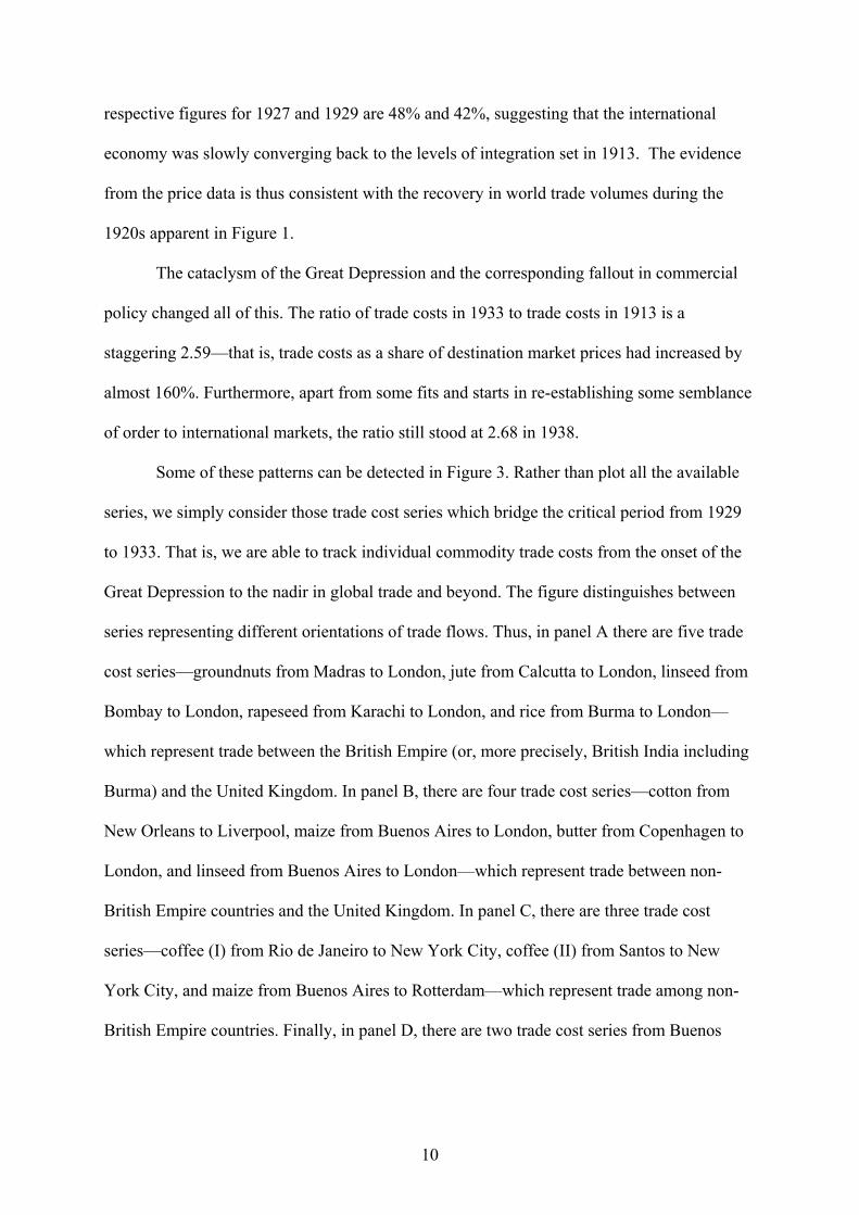
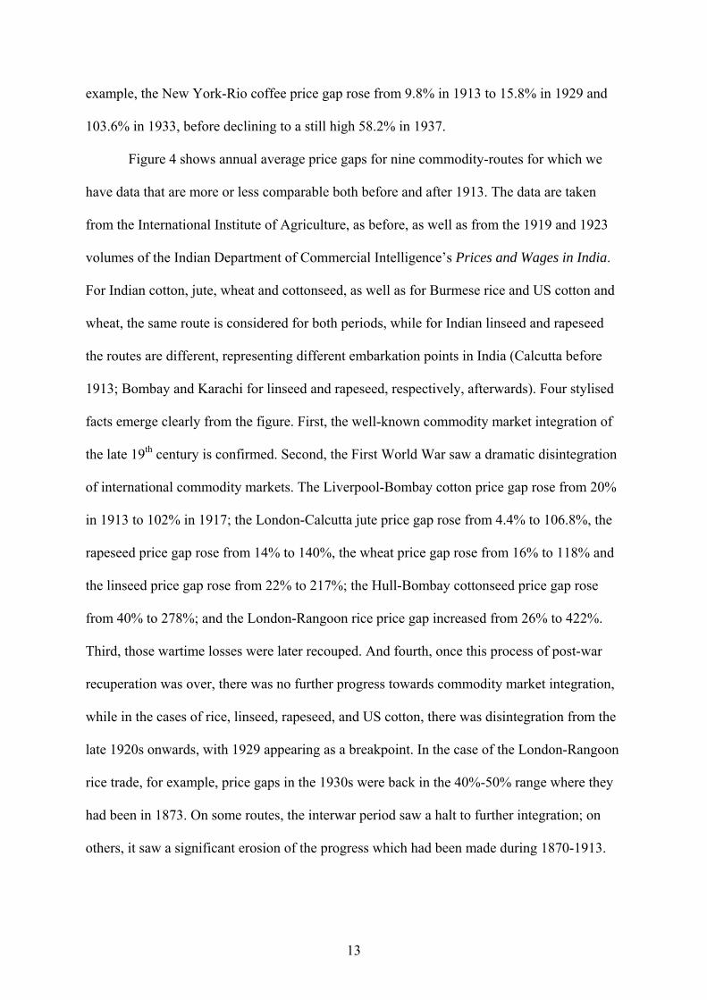
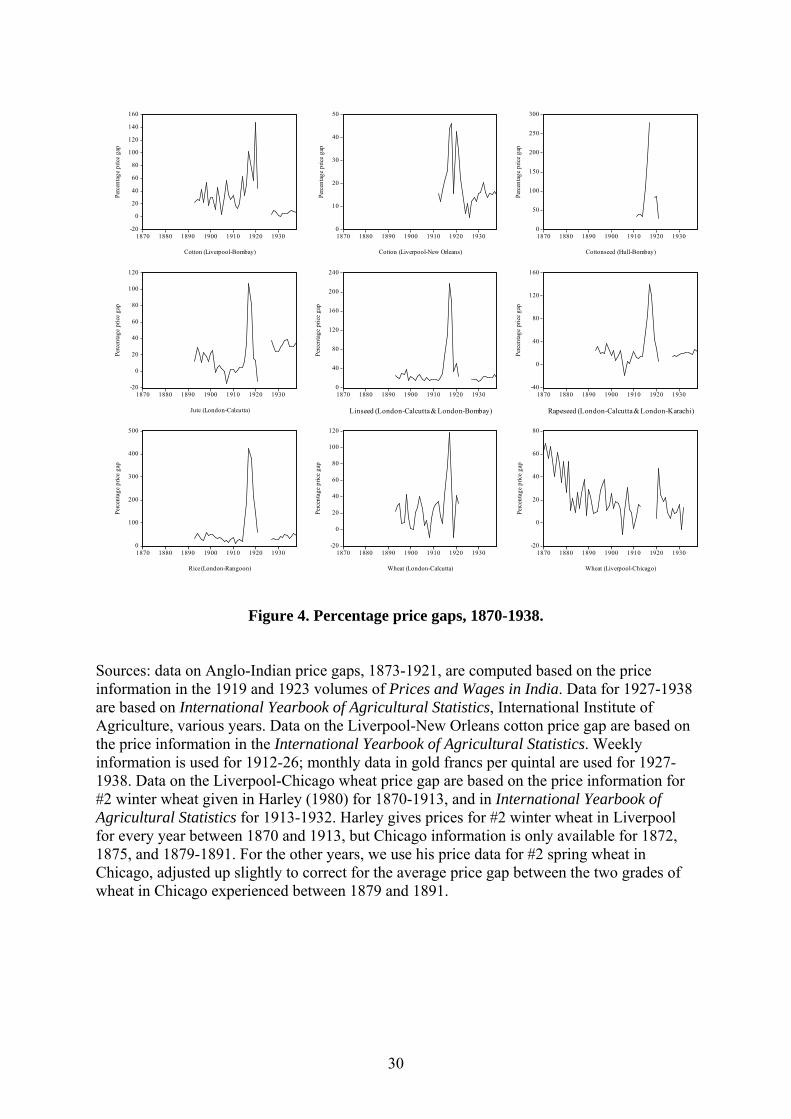
Figure 4 shows annual average price gaps for nine commodity-routes for which we

have data that are more or less comparable both before and after 1913. The data are taken

from the International Institute of Agriculture, as before, as well as from the 1919 and 1923

volumes of the Indian Department of Commercial Intelligence’s Prices and Wages in India.

For Indian cotton, jute, wheat and cottonseed, as well as for Burmese rice and US cotton and

wheat, the same route is considered for both periods, while for Indian linseed and rapeseed

the routes are different, representing different embarkation points in India (Calcutta before

1913; Bombay and Karachi for linseed and rapeseed, respectively, afterwards). Four stylised

facts emerge clearly from the figure. First, the well-known commodity market integration of

the late 19th century is confirmed. Second, the First World War saw a dramatic disintegration

of international commodity markets. The Liverpool-Bombay cotton price gap rose from 20%

in 1913 to 102% in 1917; the London-Calcutta jute price gap rose from 4.4% to 106.8%, the

rapeseed price gap rose from 14% to 140%, the wheat price gap rose from 16% to 118% and

the linseed price gap rose from 22% to 217%; the Hull-Bombay cottonseed price gap rose

from 40% to 278%; and the London-Rangoon rice price gap increased from 26% to 422%.

Third, those wartime losses were later recouped. And fourth, once this process of post-war

recuperation was over, there was no further progress towards commodity market integration,

while in the cases of rice, linseed, rapeseed, and US cotton, there was disintegration from the

late 1920s onwards, with 1929 appearing as a breakpoint. In the case of the London-Rangoon

rice trade, for example, price gaps in the 1930s were back in the 40%-50% range where they

had been in 1873. On some routes, the interwar period saw a halt to further integration; on

others, it saw a significant erosion of the progress which had been made during 1870-1913.

13

Sources of disintegration: policy or technology shocks?

One of the questions remaining is the source of this disintegration. The historical

literature strongly suggests that any changes in trade costs in the early 1930s were the result

of drastic changes in commercial policy. At the same time, the recent work of Estevadeordal,

Frantz, and Taylor (2003) suggests that there might have been some room for rising

transportation costs in explaining the interwar trade bust and, thus, the climb in estimated

trade costs.

The available evidence is ambiguous regarding what actually happened to interwar

transport costs. The interwar period saw several incremental improvements to ocean shipping

technologies, such as better boilers on steamships, or the development of turboelectric

transmission mechanisms. According to Shah Mohammed and Williamson (2004), TFP

growth in the British tramp shipping industry was as fast if not faster between 1909-11 and

1932-34 as before the war, with annual TFP growth rates of 2.83% on the transatlantic route,

1.27% on the Alexandria route, and 1.05% on the Bombay route. However, most of the

improvements had been realised by 1923-5, suggesting war-induced technological change.

Moreover, Estevadeordal et al. point out, citing Hummels (1999), that what matters for the

relative cost of shipping is its TFP growth rate relative to the economy-wide TFP growth rate

(since the latter will raise factor prices throughout the economy, and thus raise costs for

sectors experiencing below-average productivity growth).

Estevadeordal et al.’s finding that rising real maritime freight rates (from the mid­

1920s through the end of the 1930s) can help explain the interwar trade bust is based on the

Isserlis (1938) maritime freight rate index, which ends in 1936, and which they deflated by

the British consumer price index. However, there are at least two reasons why this finding

should not be accepted uncritically. The first is that the way in which Isserlis constructed his

index has been criticized, for example by Yasuba (1978) who argues that there was an

14

upward bias built into the index based on its choice of routes. The second is that if we are

concerned about the impact of freight rates on international trade, we should be deflating

them, not by a general consumer price index, but by the prices of the goods being traded.

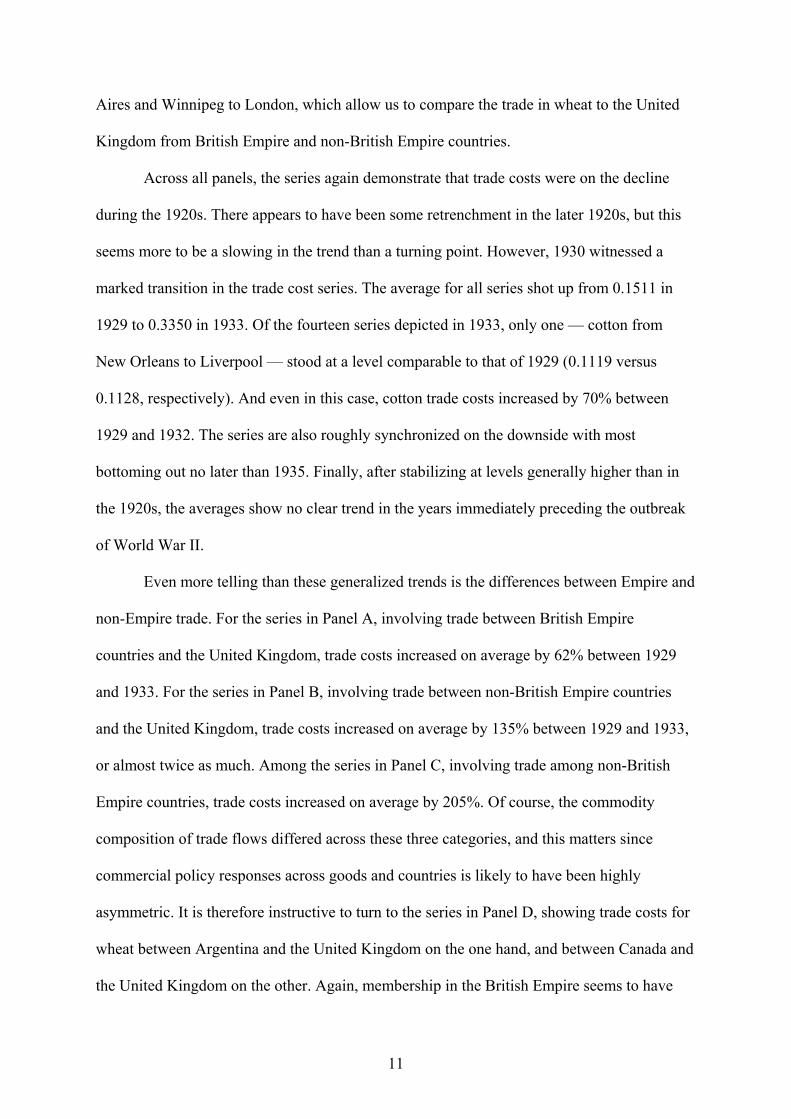
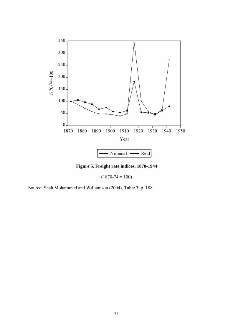
A more recent paper, by Shah Mohammed and Williamson (2004), addresses both of

these concerns. Shah Mohammed and Williamson collect freight rates for a larger and more

representative sample of routes, and deflate by route-specific deflators, based on the prices of

the commodities being shipped on those routes. The resulting nominal and real freight rate

indices, for the period 1870-1944, are plotted in Figure 5. As can be seen, despite the wartime

improvements in transportation technology mentioned earlier, freight rates shot up after 1914,

as a result of higher wages and fuel, and more expensive ships. Transport cost increases are

thus prima facie a plausible contender in explaining the wartime disintegration of

international commodity markets documented earlier. Nominal freight rates remained higher

during the 1920s than they had been before the war, although they fell continuously, and

regained pre-war levels briefly in the early 1930s. They then increased as the 1930s

progressed, before exploding once more during World War II.4

However, it is real freight rates that matter for trade, and commodity prices were

much higher after the First World War than before. The data show real freight rates falling

through the 1920s, at levels below those experienced in 1913, so that the real freight rate

index stood at 0.58 in 1930-34, as opposed to 0.75 in 1910-14. The index then increased to

0.75 in 1935-39, although how much of this rise was due to developments in 1939 is not

clear. An immediate implication of this index is that the interwar trade bust could not have

been due to rising transport costs, since real freight rates only started rising in the mid-1930s,

after world trade volumes had started to recover.

4 This evidence is consistent with the idea that because of the endogeneity between freight rates and trade flows the two series should be positively correlated—see Jacks and Pendakur (forthcoming) on this issue.

15

While the Shah Mohammed index represents the current state of the art, there is thus a

certain ambiguity regarding the course of international transport costs during the interwar

period. We therefore use our price data to gain some sense of whether or not the technology

of information transmission and goods shipment changed over that time. That is, with the

onset of the Great Depression, did commodity markets experience technological regression as

the world market imploded? We set a break-point in 1929 and estimate two TARs on all pre­

1930 observations and all post-1929 observations for two series: wheat between Buenos

Aires and London and wheat between Winnipeg and London. The choice of these two series

is strictly predicated on data availability.5

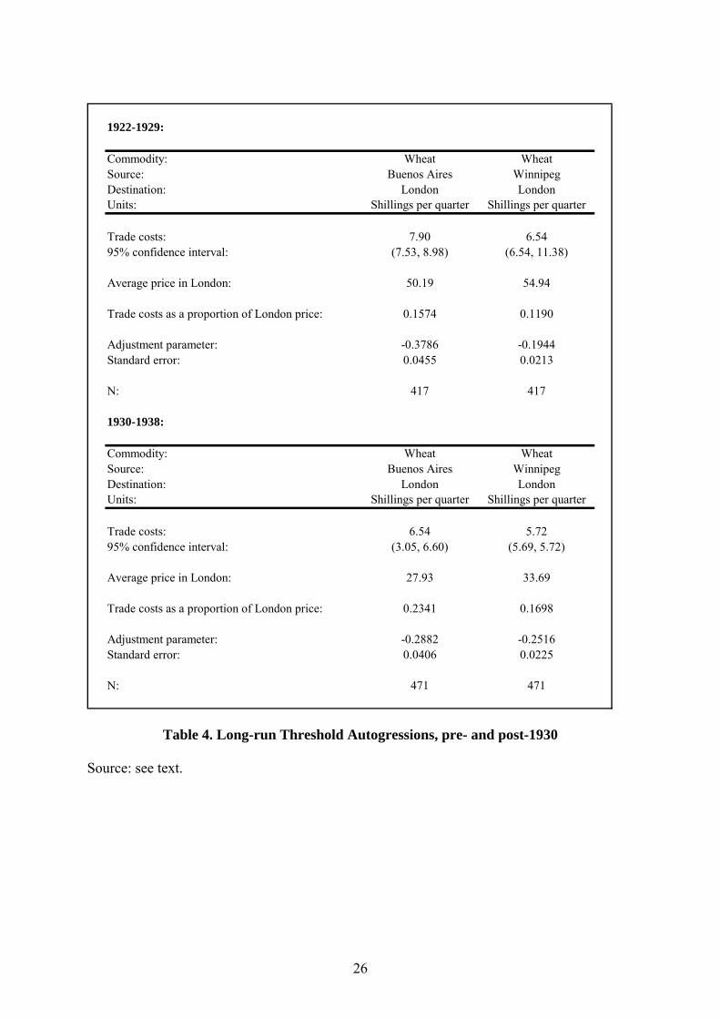
Estimating TAR models, as in equation 4.), for 1922 to 1929 and 1930 to 1938, we

generate the results reported in Table 4. In the upper panel, we find that trade costs in

shillings per quarter between 1922 and 1929 were 7.90 and 6.54 for the Buenos Aires and

Winnipeg routes, respectively. Combined with information on the average prices of the

specific varieties of wheat in London, this translates into proportional trade costs of 0.1574

and 0.1190, respectively—results which seem consistent with those in Table 2b above. The

speed of adjustment parameters are also fairly precisely estimated, at -0.3786 and -0.1944.

Turning to the post-1930 environment in the lower panel, we see that trade costs as a

proportion of the average London price increased to 0.2341 in the case of Argentine wheat

and 0.1698 in the case of Canadian wheat. At the same time, the speed of adjustment

parameter for Buenos Aires rose to -0.2882, while for Winnipeg it fell, to -0.2516. Thus,

trade costs as a proportion of London prices rose by roughly 50% in both instances.

5 The price data used in the previous section experienced gaps in reporting from August to December 1926, and from September to December 1932. That is, the observations for 1926 and 1932 previously presented were estimated over the range of January to July and January to August, respectively. This does not present a problem for estimation in a given year as the only data requirement for the TAR procedure is that the price data is evenly spaced (in this case, weekly) and continuous. However, when estimating over the entire period 1922 to 1929, or 1930 to 1938, the data need to be augmented so as to fill those gaps with observations from the latter halves of 1926 and 1932. Fortunately, the Food Research Institute’s Wheat Studies provides a wealth of data not only on consumption, production, and transactions worldwide, but also on trends in wheat prices in international markets. Combining the two sources, we have continuous weekly time series for these two wheat markets from January 1922 to December 1938.

16

Moreover, the difference is statistically significant across periods. By contrast, while the

speed of adjustment parameters do change across regimes, they do so in an inconsistent

manner, and the differences are not statistically significant. We take this as prima facie

evidence that the communication and transportation technology surrounding trade did not

change in this period, but that policy and other barriers to trade almost certainly did.

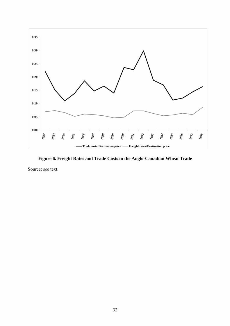
Is there any other evidence from these particular markets which might guide us on this

point? Luckily, the Wheat Studies publication also provides some limited information on

prevailing freight rates linking prominent markets in the worldwide wheat trade. In this

instance, we are limited to considering the case of the wheat trade between Winnipeg and

London. Figure 6 depicts the ratio of the estimated trade costs to the London price, and the

ratio of quoted freight rates to the London price. Both ratios start in 1922 at or near their pre­

war levels of 0.2351 and 0.0787, respectively. As in Table 2b, the trade cost to destination

price ratio falls rapidly in the early 1920s, but then remains rather steady up to 1929, when it

was 0.1382. From 1929, the trade cost series explodes, reaching a peak in 1932 of 0.2977,

and then quickly recedes by the mid-1930s. In contrast, the ratio of freight rates to the

destination price declines continuously through the 1920s with an inflection point being

reached in 1929. However, the ratio never rises above 0.1000 and is not marked by the

dramatic spike surrounding the onset of the Great Depression found in the trade cost series.

Thus, we are left with the proposition that the spikes in the proportionate trade cost series

depicted in Figure 3 must have been driven by other processes. Again, the historical literature

leads us to believe that commercial policy is a very likely contender. However, future work

should also consider the collapse of the gold standard, as well as the likely evaporation of

commercial credit in the wake of the Great Depression.

17

3. Conclusion

This paper has documented a dramatic wartime disintegration of international

commodity markets; a gradual reintegration during the 1920s; and yet another phase of

disintegration from 1929 onwards. The post-1929 disintegration was not due to increasing

freight costs, unlike the disintegration of the wartime years, and protectionism seems the

most likely alternative candidate. On the other hand, an increasing scarcity of trade finance,

similar to what is happening today, may also have been playing a role. Another possibility,

suggested by Estevadeordal, Frantz, and Taylor (2003), is that the increase in transaction

frictions associated with the collapse of the interwar gold standard may have increased trade

costs. On the other hand, the net impact of abandoning gold on trade remains to be seen,

given that, as Irwin (1993) points out, countries which maintained monetary orthodoxy were

more likely to impose quantitative restrictions on trade than those which abandoned gold.

On balance, this paper provides evidence in favour of the view that interwar

protectionism led to a severe disintegration of international commodity markets. Our hope is

that it will stimulate others to undertake the kind of work which has been extensively

undertaken for the pre-1913 period, so that we will ultimately arrive at a fuller understanding

both of 20th century trends in international integration, and of the causes of the spectacular

decline in world trade which occurred after 1929.

18

References

Balke, N.S. and T.B. Fomby. 1997. Threshold Cointegration. International Economic Review 38: 627-645.

Coleman, A. 2007. The Pitfalls of Estimating Transactions Costs from Price Data: Evidence from Trans-Atlantic Gold-Point Arbitrage, 1886–1905. Explorations in Economic History 44: 387-410.

Department of Commercial Intelligence. 1919 and 1923. Prices and Wages in India. Calcutta: Superintendent of Government Printing.

Eichengreen, B. and D.A. Irwin 1995. Trade Blocs, Currency Blocs and the Reorientation of World Trade in the 1930s. Journal of International Economics 38: 1-24.

Ejrnæs, M. and K.G. Persson. 2000. Market Integration and Transport Costs in France, 1825­1903: A Threshold Error Correction Approach to the Law of One Price. Explorations in Economic History 37: 149-173.

Engel, C. and J.H. Rogers. 2004. European Product Market Integration after the Euro. Economic Policy 39: 347-384.

Estevadeordal, A., B. Frantz and A.M. Taylor. 2003. The Rise and Fall of World Trade, 1870-1939. Quarterly Journal of Economics 118: 359-407.

Federico, G. and K.G. Persson. 2007. Market Integration and Convergence in the World Wheat Market, 1800-2000. In The New Comparative Economic History: Essays in Honor of Jeffrey G. Williamson, ed. T.J. Hatton, K.H. O'Rourke and A.M. Taylor. Cambridge, MA: MIT Press.

Federico, G. 2008. The first European grain invasion: a study in the integration of the European market 1750-1870. HEC Working Paper 2008/1. Fiesole: European University Institute.

Food Research Institute. Various years. Wheat Studies. FRI: Palo Alto.

Goldberg, P.K. and F. Verboven. 2005. Market Integration and Convergence to the Law of One Price: Evidence from the European Car Market. Journal of International Economics 65: 49-73.

Harley, C. K. 1978. Western Settlement and the Price of Wheat, 1872-1913. Journal of Economic History 38: 865-878.

Harley, C. K. 1980. Transportation, the World Wheat Trade, and the Kuznets Cycle, 1850­1913. Explorations in Economic History 17: 218-250.

Hummels, D. 1999. Have International Transportation Costs Declined? Mimeo, University of Chicago.

19

Hurd, J. 1975. Railways and the Expansion of Markets in India, 1861-1921. Explorations in Economic History 12: 263-288.

International Institute of Agriculture. Various years. International Yearbook of Agricultural Statistics. IIA: Rome.

Irwin, D.A. 1993. Multilateral and Bilateral Trade Policies in the World Trading System: An Historical Perspective. In New Dimensions in Regional Integration, ed. J. de Melo and A. Panagariya. Cambridge: Cambridge University Press.

Irwin, D.A. 1998. The Smoot-Hawley Tariff: A Quantitative Assessment. Review of Economics and Statistics 80: 326-334.

Isserlis, L. 1938. Tramp Shipping Cargoes and Freights. Journal of the Royal Statistical Society 101: 53-146.

Jacks, D.S. 2004. Market Integration in the North and Baltic Seas, 1500-1800. Journal of European Economic History 33: 285-329.

Jacks, D.S. 2005. Intra- and International Commodity Market Integration in the Atlantic Economy, 1800–1913. Explorations in Economic History 42:381-413.

Jacks, D.S. 2006. What Drove 19th Century Commodity Market Integration? Explorations in Economic History 43: 383-412.

Jacks, D.S. and K. Pendakur, forthcoming, “Global Trade and the Maritime Transport Revolution.” Review of Economics and Statistics.

Klovland, J.T. 2005. Commodity Market Integration, 1850-1913: Evidence from Britain and Germany. European Review of Economic History 9: 163-197.

Maddison, Angus. 1995. Monitoring the World Economy 1820-1992. Paris: OECD.

Madsen, J. 2001. Trade Barriers and the Collapse of World Trade during the Great Depression. Southern Economic Journal 67: 848-868

Metzer, J. 1974. Railroad Development and Market Integration: The Case of Tsarist Russia. Journal of Economic History 34: 529-550.

Obstfeld, M., and A.M. Taylor. 1997. Nonlinear Aspects of Goods-Market Arbitrage and Adjustment: Heckscher’s Commodity Points Revisited. Journal of the Japanese and International Economies 11: 441-479.

O’Rourke, K.H. 2002. Europe and the Causes of Globalization, 1790-2000. In From Europeanization of the Globe to the Globalization of Europe, ed. H. Kierzkowski. Basingstoke: Palgrave Macmillan.

O'Rourke, K.H. and J.G. Williamson. 1994. Late 19th Century Anglo-American Factor Price Convergence: Were Heckscher and Ohlin Right? Journal of Economic History 54: 892-916.

20

Özmucur, S. and Ş. Pamuk. 2007. Did European Commodity Prices Converge during 1500­1800? In The New Comparative Economic History: Essays in Honor of Jeffrey G. Williamson, ed. T.J. Hatton, K.H. O'Rourke and A.M. Taylor. Cambridge, MA: MIT Press.

Parsley, D.C. and S.-J. Wei. 2002. Currency Arrangement and Goods Market Integration: A Price Based Approach. Mimeo, Vanderbilt University and IMF.

Persson, K.G. 2004. Mind the Gap! Transport Costs and Price Convergence in the Nineteenth Century Atlantic Economy. European Review of Economic History 8: 125-147.

Shah Mohammed, S.I. and J.G. Williamson. 2004. Freight Rates and Productivity Gains in British Tramp Shipping 1869-1950. Explorations in Economic History 41: 172-203.

Tsay, R.S. 1989. Testing and Modeling Threshold Autoregressive Processes. Journal of the American Statistical Association 84: 231-240.

United Nations. 1962. International Trade Statistics 1900-1960. Mimeo, MGT(62)12 (May).

Williamson, J.G. (1974). Late Nineteenth-Century Americna Development: A General Equilibrium History. Cambridge: Cambridge University Press.

Yasuba, Y. 1978. Freight Rates and Productivity in Ocean Transportation for Japan, 1875­1943. Explorations in Economic History 15: 11-39.

21

Commodity Source Destination Years Butter, Danish for Export Copenhagen London 1913, 1927-1938 Butter, Dutch for Export Leeuwarden London 1933-1938 Coffee, No. 7 Rio Rio de Janeiro New York City 1913, 1922-1938 Coffee, No. 4 Santos Santos New York City 1927-1938 Cotton, Middling, Fair Staple, Universal Standards New Orleans Liverpool 1913, 1919-1938 Cotton, Machine Ginned Broach, Fully Good, Good Staple, Universal Standards Bombay Liverpool 1913 Cotton, Sakellaridis, Fully Good Fair, Universal Standards Alexandria Liverpool 1913, 1927-1938 Cottonseed, Upper Egyptian Alexandria London 1933-1938 Cottonseed, Sakellaridis, Good Merchandable Alexandria London 1927-1932 Eggs, Danish for Export Copenhagen London 1913, 1927-1932 Groundnuts, Coromandel, Machine Shelled Madras London 1927-1938 Jute, First Marks Calcutta London 1927-1938 Linseed, Plata, 4% Impurities Buenos Aires London 1913, 1927-1938 Linseed, Bold Bombay London 1913, 1927-1938 Maize, Yellow Plata Buenos Aires London 1913, 1922-1938 Maize, Plata Buenos Aires Rotterdam 1927-1938 Maize, No. 2 Mixed American Chicago London 1913, 1922-1926 Oats, No. 2 White Western Winnipeg London 1913, 1922-1926 Oats, No. 2 White, 49 kilograms per hectolitre Buenos Aires London 1913, 1922-1938 Rapeseed, Toria, 3% Impurities, In Bags Karachi London 1927-1938 Rice, No. 2 Burma Burma London 1913, 1927-1938 Rice, No. 1 Saigon, Round White, 25% Brokens Saigon London 1933-1938 Rye, No. 2 American Minneapolis Hamburg 1927-1932 Silk, Raw, Double Extra Cracks Yokohama New York City 1927-1932 Wheat, No. 1 Northern Manitoba Winnipeg London 1913, 1922-1938 Wheat, No. 2 Hard Winter Chicago London 1913, 1922-1932 Wheat, No. 2 Hard Buenos Aires London 1913, 1922-1938

Table 1. Commodity Coverage

22

Commodity: Butter Butter Coffee Coffee Cotton Cotton Cotton Source: Copenhagen Leeuwarden Rio Santos New Orleans Bombay Alexandria Destination: London London NYC NYC Liverpool Liverpool Liverpool

1913 0.0640 0.1271 0.0927 0.0467 0.0454

1919 0.1028 1920 0.1476 1921 0.1260 1922 0.1815 0.1194 1923 0.2060 0.1151 1924 0.1904 0.0294 1925 0.1204 0.0763 1926 0.0589 0.0990 1927 0.1007 0.1155 0.2314 0.1216 0.0464 1928 0.0659 0.0989 0.1438 0.1106 0.0353 1929 0.1032 0.1169 0.1584 0.1128 0.0287 1930 0.0935 0.2191 0.2065 0.1156 0.0281 1931 0.0943 0.1968 0.4570 0.1293 0.1294 1932 0.1372 0.3497 0.4735 0.1909 0.1380 1933 0.2415 0.2658 0.5434 0.4955 0.1119 1934 0.2646 0.3637 0.4209 0.4423 0.1124 1935 0.2248 0.2958 0.5690 0.5113 0.1357 1936 0.2137 0.2290 0.4943 0.4666 0.1194 1937 0.1956 0.1865 0.4830 0.4494 0.1504 1938 0.1900 0.1681 0.4367 0.4413 0.1134

Commodity: Cottonseed I Cottonseed II Eggs Groundnuts Jute Linseed Linseed Source: Alexandria Alexandria Copenhagen Madras Calcutta Buenos Aires Bombay Destination: London London London London London London London

1913 0.1217 0.1351

1919 1920 1921 1922 1923 1924 1925 1926 1927 0.1087 0.2335 0.1785 0.2981 0.1366 0.1543 1928 0.0954 0.1186 0.0518 0.1992 0.1214 0.1538 1929 0.1536 0.4977 0.1631 0.2056 0.1255 0.1389 1930 0.1222 0.6494 0.0828 0.1810 0.1264 0.1259 1931 0.2229 0.1705 0.2173 0.2400 0.1922 0.1623 1932 0.1528 0.5321 0.2103 0.2406 0.1904 0.2127 1933 0.2437 0.2822 0.2914 0.4450 0.1976 1934 0.2170 0.2334 0.2929 0.1500 0.1891 1935 0.1434 0.1181 0.2345 0.1232 0.2183 1936 0.2109 0.1821 0.2340 0.1525 0.2144 1937 0.2205 0.2056 0.2122 0.1641 0.2314 1938 0.1903 0.2173 0.2670 0.1489 0.2124

Table 2a. Estimated Trade Costs as a Share of Destination Market Prices

Source: see text.

23

Commodity: Maize Maize Maize Oats Oats Rapeseed Rice Source: Buenos Aires Buenos Aires Chicago Winnipeg Buenos Aires Karachi Burma Destination: London Rotterdam London London London London London

1913 0.1085 0.0884 0.3107 0.0873 0.3570

1919 1920 1921 1922 0.2632 0.2131 0.3013 0.2599 1923 0.2474 0.1161 0.3103 0.2350 1924 0.3267 0.1078 0.2425 0.1939 1925 0.1618 0.1642 0.2499 0.1668 1926 0.1728 0.1563 0.3147 0.2583 1927 0.2387 0.1771 0.4709 0.1342 0.2129 1928 0.2391 0.1935 0.4325 0.1469 0.2121 1929 0.1925 0.2154 0.4776 0.1343 0.1855 1930 0.2568 0.1652 0.5202 0.1665 0.1882 1931 0.2804 0.3921 0.6683 0.2147 0.3240 1932 0.2681 0.2399 0.5237 0.1885 0.2449 1933 0.4846 0.4448 0.2319 0.3324 1934 0.1752 0.1551 0.1859 0.3605 1935 0.2183 0.2351 0.1606 0.1857 1936 0.3242 0.2909 0.1829 0.2782 1937 0.3285 0.3016 0.2073 0.3816 1938 0.1757 0.1626 0.1821 0.3258

Commodity: Rice Rye Silk Wheat Wheat Wheat Source: Saigon Minneapolis Yokohama Winnipeg Chicago Buenos Aires Destination: London Hamburg New York City London London London

1913 0.2351 0.1194 0.1458

1919 1920 1921 1922 0.2199 0.0764 0.1969 1923 0.1507 0.0777 0.1665 1924 0.1085 0.1195 0.1251 1925 0.1376 0.1073 0.0979 1926 0.1846 0.0662 0.0308 1927 0.1686 0.0729 0.1469 0.1209 0.1246 1928 0.1553 0.1281 0.1655 0.0664 0.1223 1929 0.1387 0.1263 0.1382 0.0744 0.1258 1930 0.2446 0.0963 0.2354 0.1078 0.0630 1931 0.0944 0.1111 0.2266 0.0706 0.2488 1932 0.2307 0.0602 0.2977 0.0934 0.2048 1933 0.2665 0.1872 0.4011 1934 0.3255 0.1688 0.1540 1935 0.2591 0.1125 0.1179 1936 0.2620 0.1201 0.1626 1937 0.2718 0.1430 0.0527 1938 0.2467 0.1624 0.2191

Table 2b. Estimated Trade Costs as a Share of Destination Market Prices

Source: see text.

24

Commodity Grade Markets 1913 1922 1927 1929 1933 1937 Wheat No. 2 Winter Liverpool-Chicago 16.0 24.6 12.9 8.7 Wheat No. 1 Northern Manitoba London-Winnipeg 24.5 34.7 7.7 9.9 20.7 17.7 Wheat Plate London-Buenos-Aires 9.0 26.3 11.0 11.6 10.1 5.8 Maize Plate London-Buenos-Aires 18.7 39.3 25.3 21.0 25.5 33.6 Oats Plate London-Buenos-Aires 13.5 33.2 29.1 25.7 26.0 Rice Birmanie No. 4 London-Rangoon 25.9 27.7 50.4 55.3 Rice Saigon No. 1 London-Saigon 76.2 39.7 39.0 44.2 Rapeseed Toria London-Karachi 14.7 15.1 21.8 27.3 Groundnut Coromandel London-Madras 20.5 15.2 27.1 26.6 Linseed Bombay London-Bombay 17.6 16.8 23.9 27.9 Linseed La Plata London-Buenos-Aires 16.0 14.7 13.1 22.2 Cotton Middling Liverpool-New Orleans 12.0 22.1 12.2 12.2 15.9 16.5 Cotton Broach Liverpool-Bombay 4.0 8.4 5.4 8.8 Cotton Sakellaridas London-Alexandria 6.2 5.4 13.0 10.1 Cottonseed Sakellaridas London-Alexandria 17.5 19.8 23.8 24.2 Eggs Danish London-Denmark 43.6 58.7 71.5 73.8 Eggs Dutch London-Holland 12.8 23.6 15.4 45.7 Butter Danish London-Copenhagen 7.9 10.1 36.7 24.7 Coffee Rio No. 7 New York-Rio 9.8 17.0 15.5 15.8 103.6 58.2 Coffee Santos No. 4 New York-Santos 28.0 19.3 89.8 55.8

Table 3. Average annual commodity price gaps, 1913-1937 (percent)

Source: International Yearbook of Agricultural Statistics, International Institute of Agriculture, various years. Data for 1927-37 are based on annual averages of monthly price data, expressed in gold francs per quintal. There are two exceptions: such monthly price data are only available for Liverpool-Chicago wheat prices for 1927-32; and for London-Buenos Aires oats prices for 1927-33. Where monthly data in gold francs per quintal are not available, price gaps are calculated based on the weekly price data used elsewhere in this paper.

25

1922-1929:

Commodity: Wheat Wheat Source: Buenos Aires Winnipeg Destination: London London Units: Shillings per quarter Shillings per quarter

Trade costs: 7.90 6.54 95% confidence interval: (7.53, 8.98) (6.54, 11.38)

Average price in London: 50.19 54.94

Trade costs as a proportion of London price: 0.1574 0.1190

Adjustment parameter: -0.3786 -0.1944 Standard error: 0.0455 0.0213

N: 417 417

1930-1938:

Commodity: Wheat Wheat Source: Buenos Aires Winnipeg Destination: London London Units: Shillings per quarter Shillings per quarter

Trade costs: 6.54 5.72 95% confidence interval: (3.05, 6.60) (5.69, 5.72)

Average price in London: 27.93 33.69

Trade costs as a proportion of London price: 0.2341 0.1698

Adjustment parameter: -0.2882 -0.2516 Standard error: 0.0406 0.0225

N: 471 471

Table 4. Long-run Threshold Autogressions, pre- and post-1930

Source: see text.

26

50

60

70

80

90

100

110

120 19

29=

100

1910 1915 1920 1925 1930 1935 1940 1945 1950

Maddison UN

Figure 1. World trade indices, 1913-1950

(1929=100)

Source: United Nations (1962), Maddison (1995, p. 239).

27

0

2

4

6

8

10

12

14

1 3 5 7 9 11 13 15 17 19 21 23 25 27 29 31 33 35 37 39 41 43 45 47 49 51

Price margin Trade cost 95% CI, lower 95% CI, upper

Figure 2. Price Margins in the Market for Danish Butter, 1913 (shillings/hundredweight)

Source: see text.

28

0.00

0.10

0.20

0.30

0.40

0.50

0.60

1913

1919

19

20

1921

19

22

1923

19

24

1925

19

26

1927

19

28

1929

19

30

1931

19

32

1933

19

34

1935

19

36

1937

19

38

Groundnuts Jute Linseed Rapeseed Rice

0.00

0.10

0.20

0.30

0.40

0.50

0.60

1913

1919

19

20

1921

19

22

1923

19

24

1925

19

26

1927

19

28

1929

19

30

1931

19

32

1933

19

34

1935

19

36

1937

19

38

Cotton Maize Butter Linseed

Panel A: British Empire to the UK Panel B: Non-Empire to the UK

0.00

0.10

0.20

0.30

0.40

0.50

0.60

1913

1919

19

20

1921

19

22

1923

19

24

1925

19

26

1927

19

28

1929

19

30

1931

19

32

1933

19

34

1935

19

36

1937

19

38

Coffee I Coffee II Maize

0.00

0.10

0.20

0.30

0.40

0.50

0.60

1913

1919

19

20

1921

19

22

1923

19

24

1925

19

26

1927

19

28

1929

19

30

1931

19

32

1933

19

34

1935

19

36

1937

19

38

Argentine Canadian

Panel C: Non-Empire to Non-Empire Panel D: Wheat to the UK Figure 3. Trade Costs, 1913, 1919-1938

29

160 50 300

140

120 40 250

100 200 30

Perc

enta

ge p

rice

gap

Perc

enta

ge p

rice

gap

Perc

enta

ge p

rice

gap

Perc

enta

ge p

rice

gap

Perc

enta

ge p

rice

gap

Perc

enta

ge p

rice

gap

Perc

enta

ge p

rice

gap

Perc

enta

ge p

rice

gap

Perc

enta

ge p

rice

gap

80

60

40

150

100 20

20 10 50

0

-20 0 0 1870 1880 1890 1900 1910 1920 1930 1870 1880 1890 1900 1910 1920 1930 1870 1880 1890 1900 1910 1920 1930

Cotton (Liverpool-Bombay) Cotton (Liverpool-New Orleans) Cottonseed (Hull-Bombay)

120 240 160

100 200 120

80

60

40

20

160

120

80

80

40

00 40

-20 0 -40 1870 1880 1890 1900 1910 1920 1930 1870 1880 1890 1900 1910 1920 1930 1870 1880 1890 1900 1910 1920 1930

Jute (London-Calcutta) Linseed (London-Calcutta & London-Bombay) Rapeseed (London-Calcutta & London-Karachi)

500 120 80

100 400 60

80

60

40

20

300

200

40

20

100 0 0

0 -20 -20 1870 1880 1890 1900 1910 1920 1930 1870 1880 1890 1900 1910 1920 1930 1870 1880 1890 1900 1910 1920 1930

Rice (London-Rangoon) Wheat (London-Calcutta) Wheat (Liverpool-Chicago)

Figure 4. Percentage price gaps, 1870-1938.

Sources: data on Anglo-Indian price gaps, 1873-1921, are computed based on the price information in the 1919 and 1923 volumes of Prices and Wages in India. Data for 1927-1938 are based on International Yearbook of Agricultural Statistics, International Institute of Agriculture, various years. Data on the Liverpool-New Orleans cotton price gap are based on the price information in the International Yearbook of Agricultural Statistics. Weekly information is used for 1912-26; monthly data in gold francs per quintal are used for 1927­1938. Data on the Liverpool-Chicago wheat price gap are based on the price information for #2 winter wheat given in Harley (1980) for 1870-1913, and in International Yearbook of Agricultural Statistics for 1913-1932. Harley gives prices for #2 winter wheat in Liverpool for every year between 1870 and 1913, but Chicago information is only available for 1872, 1875, and 1879-1891. For the other years, we use his price data for #2 spring wheat in Chicago, adjusted up slightly to correct for the average price gap between the two grades of wheat in Chicago experienced between 1879 and 1891.

30

350

0

50

100

150

200

250

300

1870 1880 1890 1900 1910 1920 1930 1940 1950

1870

-74=

100

Year

Nominal Real

Figure 5. Freight rate indices, 1870-1944

(1870-74 = 100)

Source: Shah Mohammed and Williamson (2004), Table 3, p. 188.

31

0.00

0.05

0.10

0.15

0.20

0.25

0.30

0.35

1922

1923

1924

1925

1926

1927

1928

1929

1930

1931

1932

1933

1934

1935

1936

1937

1938

Trade costs/Destination price Freight rates/Destination price

Figure 6. Freight Rates and Trade Costs in the Anglo-Canadian Wheat Trade

Source: see text.

32