combining heuristics for the economic lot-sizing problem · abstract this report shows a new...

Bachelor Thesis Econometrie & Besliskunde 2008/2009

Combining Heuristics For The

Economic Lot-Sizing Problem

Charlie Ye (302759)

Supervisor: Dr. Wilco van den Heuvel

August 3, 2009

Abstract

This report shows a new heuristic for the economic lot-sizing problem (ELSP)

made by combining two already existing heuristics, namely a modification of the

well-known part-period algorithm (PPA) by DeMatteis (1968) and a fairly new

heuristic by Van den Heuvel and Wagelmans (2009b). The performance of this

new heuristic will be tested against a variety of heuristics of the same order and

the optimal solution obtained from the Wagner-Whitin algorithm. This will be

done in both a static schedule and a rolling horizon context.

Contents

1 Introduction 3

2 Wagner-Whitin Algorithm 6

2.1 Assumptions . . . . . . . . . . . . . . . . . . . . . . . . . . . . . . . 6

2.2 Wagner-Whitin algorithm . . . . . . . . . . . . . . . . . . . . . . . 8

2.3 Constrained Wagner-Whitin . . . . . . . . . . . . . . . . . . . . . . 10

2.4 Wagner-Whitin heuristic . . . . . . . . . . . . . . . . . . . . . . . . 11

3 Heuristics 12

3.1 Class of heuristics . . . . . . . . . . . . . . . . . . . . . . . . . . . . 12

3.2 Existing heuristics . . . . . . . . . . . . . . . . . . . . . . . . . . . 13

3.2.1 Part-period algorithm (PPA) . . . . . . . . . . . . . . . . . 13

3.2.2 Silver-Meal . . . . . . . . . . . . . . . . . . . . . . . . . . . 15

3.2.3 Least Unit Cost (LUC) . . . . . . . . . . . . . . . . . . . . . 16

3.2.4 Heuristic H* . . . . . . . . . . . . . . . . . . . . . . . . . . . 16

3.3 New heuristic (PPA-H*) . . . . . . . . . . . . . . . . . . . . . . . . 17

4 Performance 21

4.1 Static schedule . . . . . . . . . . . . . . . . . . . . . . . . . . . . . 21

4.1.1 Standard data set . . . . . . . . . . . . . . . . . . . . . . . . 22

4.1.2 Simulated data sets . . . . . . . . . . . . . . . . . . . . . . . 22

4.1.3 Manually constructed data set . . . . . . . . . . . . . . . . . 24

4.2 Rolling horizon . . . . . . . . . . . . . . . . . . . . . . . . . . . . . 24

4.3 Variations on PPA-H* . . . . . . . . . . . . . . . . . . . . . . . . . 26

4.3.1 In the static schedule . . . . . . . . . . . . . . . . . . . . . . 27

1

CONTENTS 2

4.3.2 In the rolling horizon schedule . . . . . . . . . . . . . . . . . 27

5 Conclusion and future research 30

Chapter 1

Introduction

Dynamic lot-sizing determines the amount and timing of an order (or production)

of a good that can be stored. This involves order cost and holding (or storage)

cost. Order cost is the cost for ordering a batch of goods once. Holding cost is

the cost to keep and maintain a batch of goods in storage for a certain amount of

time. Holding costs can include the rent for the space that is needed to store the

items in, the heating or cooling that is needed to keep the items from deteriorating,

security, et cetera.

One can choose to order goods in every period where the goods are demanded.

This will result in a total cost equal to the order cost multiplied by the number

of periods, thus with zero holding cost. But because the goods can be stored, one

can also choose to order only once, ordering the total quantity that is needed over

all periods. This causes a decrease in the total order cost, but will dramatically

increase the total holding cost, as the goods have to be stored over multiple periods.

Obviously, one wants to minimize the total costs. Because there is a trade-off

between the number of times one orders and the quantity that is ordered every

time, there exists a combination such that the total costs will be minimized. The

solution is dependent on the order cost, the holding cost for one period and the

demand pattern over all periods.

This problem can be solved optimally by an algorithm introduced by Wag-

ner and Whitin (1958). Although this algorithm can solve lot-sizing problems

optimally, it is rarely used in practice. A reason for this is that the algorithm

3

CHAPTER 1. INTRODUCTION 4

is relatively complex, making it more difficult to understand than other meth-

ods. Also, the Wagner-Whitin algorithm only gives guaranteed optimal solution

in static schedules. In a static schedule, the ending point is well-defined and no

future demands will become available. The demand for each period from the first

period through the last period, the ending point, is known. This is called the

horizon. In a static schedule, the information of the whole horizon can be used to

determine a solution. We say that the planning horizon is equal to the horizon.

In practice, the information of the whole horizon is not available. It is hard

to predict when one will not be needed to order anymore. Even if this piece of

information would be available, the demand pattern up to that period will be

hard to predict, if not impossible. Therefore, a rolling horizon schedule is used in

practice. In a rolling horizon schedule, the information of only a limited number of

periods is available at a certain period. As time progresses, more information will

become available. Predicting the demand quantities for the near future, or even

know them through accumulated orders, is much more feasible in practice than

to predict the demand quantities for a large number of periods. For example, at

period 1 the demand quantities of periods 1 through 5 are known and can be used

to obtain a replenishment strategy. At period 2, the demand quantity of period 6

will become available. So at period 2, the information of period 2 through 6 can

be used. This can continue indefinitely, which is what happens in practice, where

an ending point is normally not known. The horizon in this example, as well as

the planning horizon, is equal to 5. In this work however, we know the demand

patterns beforehand. This means the horizon in the rolling horizon schedule is the

same as the horizon in the static schedule. However, the planning horizon in the

rolling horizon schedule will be significantly smaller than the horizon, whereas in

a static schedule the planning horizon is equal to the horizon. This ensures that

the rolling horizon application will act the same as it would in practice, where the

horizon would be smaller.

To solve the lot-sizing problem without having the drawbacks of the Wagner-

Whitin algorithm, heuristics were introduced. In this work we first discuss the

Wagner-Whitin algorithm. Then we show some well-known heuristics and intro-

duce a new heuristic which is based on two existing heuristics. The performance

of the new heuristic will be compared to that of the Wagner-Whitin algorithm and

CHAPTER 1. INTRODUCTION 5

the old heuristics. This will be done in both a static schedule and a rolling horizon

schedule. Finally, we will show the performance of several variations on the new

heuristic.

Chapter 2

Wagner-Whitin Algorithm

Wagner and Whitin (1958) developed an algorithm that guarantees an optimal

solution for the lot-sizing problem under a set of general assumptions. In this

work we will use three versions of the Wagner-Whitin algorithm. First of all, the

classic Wagner-Whitin algorithm will be presented, which gives an optimal solution

in a static schedule. In a rolling horizon schedule, the results of the classic Wagner-

Whitin algorithm will not be appropriate anymore to compare the heuristics to,

since the heuristics will have additional assumptions which the Wagner-Whitin

algorithm does not have to comply to. Therefore we will also use a constrained

Wagner-Whitin algorithm, which is adapted to the rolling horizon setting, making

it comparable to the heuristics. Finally, we will use the Wagner-Whitin algorithm

as a heuristic.

2.1 Assumptions

The following assumptions apply to the Wagner-Whitin algorithm as well as the

heuristics stated in this work. These assumptions are slightly modified versions of

those from Silver et al. (1998).

1. The demand rate is given in the form of Dj which has to be satisfied in

period j (j = 1, 2, . . . , N) where the planning horizon is at the end of period

N . The demand rate may vary from period to period, unlike in a steady

6

CHAPTER 2. WAGNER-WHITIN ALGORITHM 7

state where an economic order quantity (EOQ) can be used, but is assumed

known.

2. The entire requirements of each period must be available at the beginning of

that period. Therefore, a replenishment arriving part-way through a period

cannot be used to satisfy that period’s requirements. It is cheaper, in terms

of reduced carrying costs, to delay its arrival until the start of the next

period. Thus, replenishments are constrained to arrive at the beginnings of

periods.

3. The cost factors do not change appreciably with time; in particular, inflation

is at a negligibly low level.

4. The item is treated entirely independently of other items; that is, benefits

from joint review or replenishment do not exist or are ignored.

5. The replenishment lead time is known with certainty (a special case being

zero duration) so that delivery can be timed to occur right at the beginning

of a period.

6. No shortages are allowed.

7. The entire order quantity is delivered at the same time.

8. It is assumed that the carrying cost is only applicable to inventory that is

carried over from one period to the next.

9. Orders will only be started in periods which have nonzero demand. It is

obviously not optimal to start an order in a period with zero demand. If

the replenishment is only for that period, the order cost is paid for nothing.

If the replenishment is for multiple periods, unnecessary holding costs are

made. In both situations it is better to start an order in the first upcoming

period with nonzero demand.


2.2 Wagner-Whitin algorithm

The Wagner-Whitin algorithm needs an additional assumption to guarantee an

optimal solution. It has to be assumed that the demand pattern terminates at

the planning horizon. If it does not terminate at the planning horizon, future de-

mands may influence the ordering periods that are established within the planning

horizon. This will lead to the need of rescheduling and the previously established

order periods will not be guaranteed to be optimal anymore.

The algorithm is an application of dynamic programming, a mathematical

procedure for solving sequential decision problems. This is because the outcome

of an order at one point has effects on the possible replenishment actions that can

be taken at later decision times. The algorithm first looks at all the possibilities

in a period and calculates the according costs. This is done for all periods. For

example, in period 1, one can only choose to place an order (if the demand at period

1 is nonzero). If the minimum possible cost of periods 1 through t is defined by

Ft, F1 would be equal to the order cost A.

In period 2, one can either use the best option up until period 1 (start an order in

period 1, which is the only option) and start another order in period 2, resulting

in costs of F1 + A = 2 · A, or decide to order the demand quantity of period 2

already in period 1. This results in holding costs being made in period 1, since

the quantity ordered in period 1 for period 2 has to be stored for whole period 1.

The total cost for this option is equal to A + D2 · h · 1, with h the holding cost per

unit per period. F2 would then be the minimum out of these two options.

In period 3, there are three options that can be considered. First is to use the

best option up until period 2 and start a new order in period 3, replenishing only

D3. The cost for this option will be F2 + A. Second, one can use the best option

up until period 1 and start an order in period 2 that replenishes D2 as well as

D3. This results in a cost of F1 + A + D3 · h · 1. The third option is to have a

single order in period 1 that replenishes the whole demand quantity from period

1 through 3. The cost for this option is A + D2 · h · 1 + D3 · h · 2. Notice that

the demand quantity of period 3 has to be stored for two periods, doubling the

holding cost for the demand quantity of period 3. This continues for all periods

in the planning horizon.


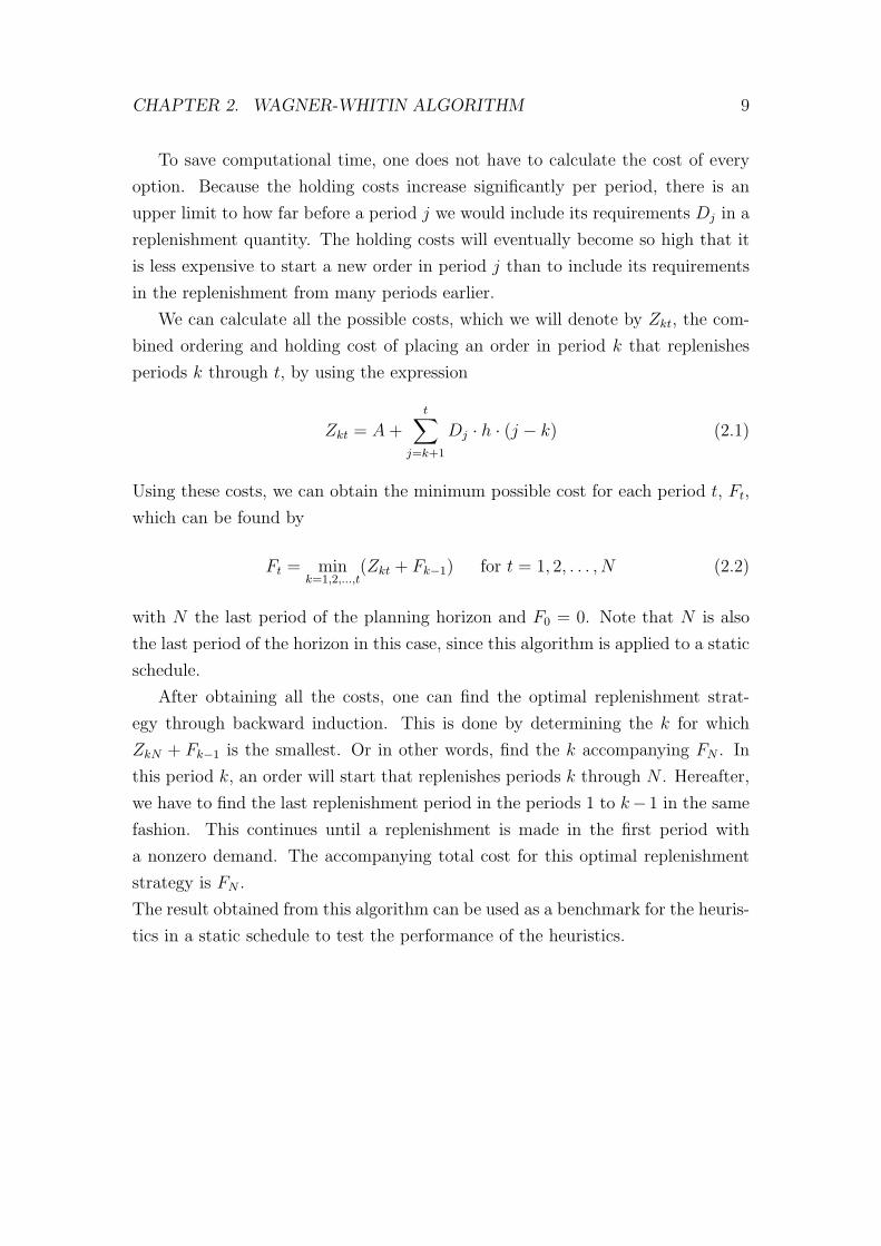
To save computational time, one does not have to calculate the cost of every

option. Because the holding costs increase significantly per period, there is an

upper limit to how far before a period j we would include its requirements Dj in a

replenishment quantity. The holding costs will eventually become so high that it

is less expensive to start a new order in period j than to include its requirements

in the replenishment from many periods earlier.

We can calculate all the possible costs, which we will denote by Zkt, the com-

bined ordering and holding cost of placing an order in period k that replenishes

periods k through t, by using the expression

Zkt = A +t∑

j=k+1

Dj · h · (j − k) (2.1)

Using these costs, we can obtain the minimum possible cost for each period t, Ft,

which can be found by

Ft = mink=1,2,...,t

(Zkt + Fk−1) for t = 1, 2, . . . , N (2.2)

with N the last period of the planning horizon and F0 = 0. Note that N is also

the last period of the horizon in this case, since this algorithm is applied to a static

schedule.

After obtaining all the costs, one can find the optimal replenishment strat-

egy through backward induction. This is done by determining the k for which

ZkN + Fk−1 is the smallest. Or in other words, find the k accompanying FN . In

this period k, an order will start that replenishes periods k through N . Hereafter,

we have to find the last replenishment period in the periods 1 to k− 1 in the same

fashion. This continues until a replenishment is made in the first period with

a nonzero demand. The accompanying total cost for this optimal replenishment

strategy is FN .

The result obtained from this algorithm can be used as a benchmark for the heuris-

tics in a static schedule to test the performance of the heuristics.


2.3 Constrained Wagner-Whitin

In a rolling horizon schedule, the solution from the Wagner-Whitin algorithm loses

meaning because no heuristic can get close to it under rolling horizon conditions.

Therefore we make use of the so-called constrained Wagner-Whitin algorithm. This

algorithm works in the same way as the Wagner-Whitin algorithm with a minor

modification to account for a planning horizon which is smaller than the horizon.

Instead of choosing the minimum cost in period t, Ft, from the costs of periods 1

through t, the algorithm is constrained to only use the costs of periods t−N + 1

through t, given that t − N + 1 is positive and period t has a nonzero demand.

If t − N + 1 is nonpositive, then one can use the costs of periods 1 through t. If

period t contains a zero demand, then the first period with nonzero demand before

period t is chosen as the last period the algorithm can use info from, say period s,

and the algorithm can use the costs of periods s−N + 1 through s. In this way,

no order is permitted to span a length of time longer than the planning horizon

used in the heuristics.

If this is done over the whole demand pattern, the result is the lowest cost

schedule, given an explicit constraint of the simulation environment that is used

for the heuristics. The optimal replenishment strategy can again be found by

backward induction and the accompanying total cost is FT , with T the last period

of the horizon.

The constraint imposed in this constrained application of the Wagner-Whitin

algorithm modifies expression (2.2) into

Ft = mink=p,p+1,...t

(Zkt + Fk−1) for t = 1, 2, . . . , T (2.3)

where p = 1 if t ≤ N and p = t−N + 1 otherwise.

The result from this constrained application of the Wagner-Whitin algorithm

can be used as a benchmark for the heuristics in a rolling horizon schedule in the

same way the Wagner-Whitin algorithm is used as a benchmark in the case of a

static schedule.


2.4 Wagner-Whitin heuristic

There is also the possibility to use the Wagner-Whitin algorithm as a heuristic.

The heuristic starts in the first period with nonzero demand, say period t, where

an order will start. It then uses information of N periods, with N the length of

the planning horizon, to apply the Wagner-Whitin algorithm on. So it determines

the optimal solution for period t through t + N − 1. Through backward induction

the optimal replenishment strategy is determined for this subproblem. The period

in which the next replenishment occurs, that is, the first period after period t in

which a replenishment occurs, is selected as the new t. The minimum possible cost

up until the new period t is stored in Ft and an order will start in period t. Then

the algorithm repeats itself until the end of the horizon is reached.

In the case no replenishment is found in the subproblem apart from the replen-

ishment at period t (the first period of the subproblem), the next replenishment

will be in the first period with nonzero demand after period t + N − 1. This way,

no order is permitted to span a length of time longer than the planning horizon.

Obviously, this heuristic can only be used in the rolling horizon setting, where

the planning horizon is smaller than the horizon. In a static schedule, the length

of the planning horizon is equal to the length of the horizon, which will result in

the heuristic being the same as the original Wagner-Whitin algorithm.

Chapter 3

Heuristics

After the introduction of the Wagner-Whitin algorithm in 1958, heuristics were

developed that try to obtain solutions as close to the optimal solution as possible.

The Wagner-Whitin algorithm was being used primarily as benchmark against

which to evaluate heuristics.

3.1 Class of heuristics

There are many kinds of heuristics developed for the ELSP, mainly dating from late

1960s to early 1980s (Simpson, 2001). The class of heuristics we will be focusing

on in this report is the same class of on-line heuristics as defined in Van den Heuvel

and Wagelmans (2009a).

Definition The on-line lot-sizing heuristics make setup decisions period by period

(so previously made decisions are fixed and cannot be changed) and setup decisions

do not depend on future demand.

In other words, in period t one must decide whether to start an order (or setup)

or not, depending on the demand available from period 1 to t. Once a decision is

made, it can not be altered again in a future period. All the heuristics presented

in this report comply to this definition.

12

CHAPTER 3. HEURISTICS 13

3.2 Existing heuristics

Before we go on to the actual heuristics, we first have to define the terms used in

the explanation of the heuristics, since the notation differs from article to article.

We assume period 1 is the period in which an order will take place. The number

of periods which this order will have to supply, the lot size, is denoted by t. Once t

is decided, the next non-zero demand period, where a new order will have to start,

will become the new period 1. (In the H* and PPA-H* heuristics however, t is

defined slightly differently.) The period before the period where a new order will

have to start, or the number of periods that gets covered by all previous orders, is

denoted by k (note the slight difference compared to Wagner-Whitin). This will

be repeated until the end of the horizon. The order cost will be denoted by A.

The total holding cost of a lot will be denoted by

H1,t =t∑

i=1

Dk+i · h · i (3.1)

where Dk+i is the demand at period k + i and h is the holding cost per unit per

period.

To obtain a better understanding of the heuristics, we will apply the heuristics

to a numerical example. This problem will consist of 12 periods and the demand

pattern is given by

Period 1 2 3 4 5 6 7 8 9 10 11 12Demand 250 10 20 250 10 20 20 250 15 10 20 230

Table 3.1: Demand pattern over 12 periods

The order cost will be 206 and the holding cost per unit per period will be 2.

The optimal solution obtained from the Wagner-Whitin algorithm can be found

in Table 3.2, which will be used as a benchmark.

3.2.1 Part-period algorithm (PPA)

In 1968 DeMatteis introduced the part-period algorithm. This algorithm keeps

adding demand quantities to an order as long as the total holding cost H1,t in the


Period 1 2 3 4 5 6 7 8 9 10 11 12Demand 250 10 20 250 10 20 20 250 15 10 20 230Replen. 280 — — 300 — — — 295 — — — 230Total cost 206 226 306 512 532 612 732 938 968 1008 1128 1334

Table 3.2: Optimal solution obtained from the Wagner-Whitin Algorithm

lot remains below or equal to the order cost A. So the stopping condition becomes

H1,t ≤ A < H1,t+1 (3.2)

An other form of this algorithm can be obtained by making a small modification

to the stopping rule, such that it becomes

H1,t < A ≤ H1,t+1 (3.3)

This modification is referred to as PPA(–) by Baker (1989), since it results in

smaller lot sizes in general compared to the original PPA.

Another modification is to stop adding quantities when the total holding cost

H1,t is made as close as possible to the order cost A. In other words, stop adding

quantities at either period t if

|A−H1,t| < |A−H1,t+1| (3.4)

or at period t + 1 if

|A−H1,t+1| < |A−H1,t| (3.5)

At exact equality the PPA stopping rule will be applied. This modification is

called part-period balancing (PPB) by Silver et al. (1998).

In literature, the terms PPA and PPB are used interchangeably. This causes

confusion, since it is often not clear which variation of the algorithm is meant. In

this report, the aforementioned terms will be used to refer to their corresponding

variation.

Because the PPA(–) variation of this heuristic will be used throughout this

report, we will apply PPA(–) on the numerical example. The results can be found

in Table 3.3. The holding costs in this table are the supposed holding costs, the


holding costs if the period was to be added to the last lot. These holding costs

can then be compared to the order cost and one can decide whether to start

an order in that period or not. One can see that the total holding cost of the lot

beginning in period 4 surpasses the order cost in period 7, resulting in an additional

replenishment in period 7 and a higher total cost compared to the optimal solution.

So PPA(–) gives a non-optimal solution in this particular example.

Period 1 2 3 4 5 6 7 8 9 10 11 12Demand 250 10 20 250 10 20 20 250 15 10 20 230Hold. cost 0 20 100 1600 20 100 220 500 30 70 190 460Replen. 280 — — 280 — — 20 295 — — — 230Total cost 206 226 306 512 532 612 818 1024 1054 1094 1214 1420

Table 3.3: Results of using the PPA(–) variation of the part period algorithm

3.2.2 Silver-Meal

The Silver-Meal algorithm appeared shortly after (Silver and Meal, 1973). In this

algorithm, one wishes to choose a t, the number of periods an order lasts, which

minimizes the total relevant costs per unit time (TRCUT(t)). The TRCUT(t) can

be found by

TRCUT (t) =A + H1,t

t(3.6)

The heuristic evaluates TRCUT(t) for increasing values of t until

TRCUT (t + 1) > TRCUT (t) (3.7)

for the first time. The associated t selected by this method represents the number

of periods the replenishment of that specific lot should cover. A drawback of this

method is that it will only ensure a local minimum in the total relevant costs per

unit time, for the current replenishment, as mentioned by Silver et al. (1998).

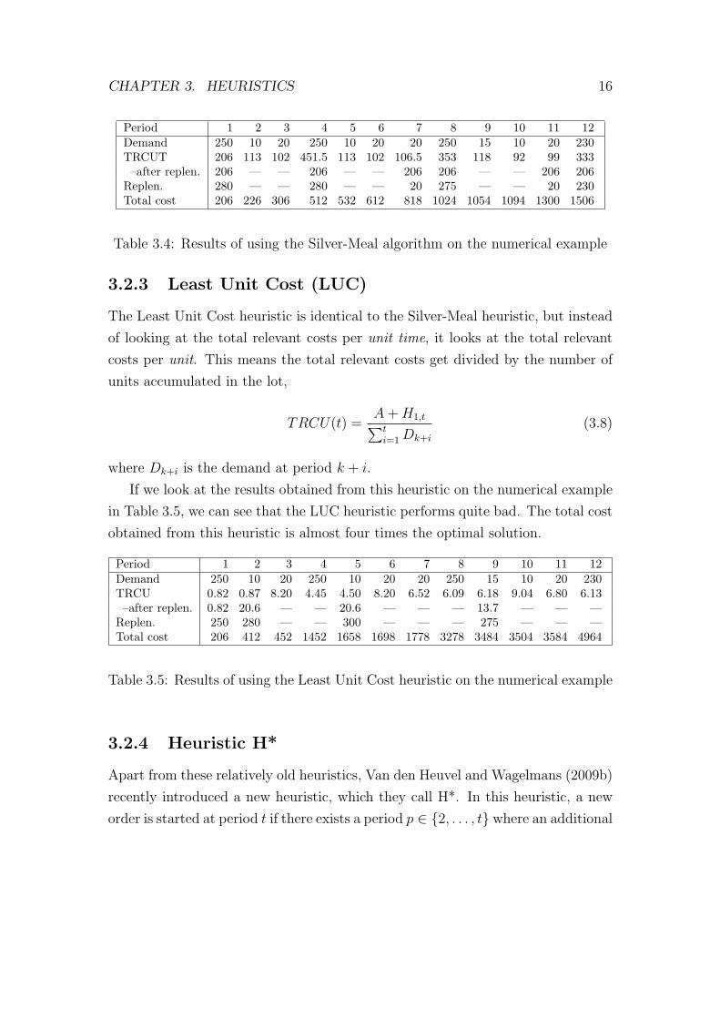
The results of using the Silver-Meal algorithm on the numerical example can

be found in Table 3.4. Notice the relatively small increases in TRCUT in periods

7 and 11, which cause new orders to start in those periods, resulting in even larger

expenses than PPA(–).


Period 1 2 3 4 5 6 7 8 9 10 11 12Demand 250 10 20 250 10 20 20 250 15 10 20 230TRCUT 206 113 102 451.5 113 102 106.5 353 118 92 99 333

–after replen. 206 — — 206 — — 206 206 — — 206 206Replen. 280 — — 280 — — 20 275 — — 20 230Total cost 206 226 306 512 532 612 818 1024 1054 1094 1300 1506

Table 3.4: Results of using the Silver-Meal algorithm on the numerical example

3.2.3 Least Unit Cost (LUC)

The Least Unit Cost heuristic is identical to the Silver-Meal heuristic, but instead

of looking at the total relevant costs per unit time, it looks at the total relevant

costs per unit. This means the total relevant costs get divided by the number of

units accumulated in the lot,

TRCU(t) =A + H1,t∑t

i=1 Dk+i

(3.8)

where Dk+i is the demand at period k + i.

If we look at the results obtained from this heuristic on the numerical example

in Table 3.5, we can see that the LUC heuristic performs quite bad. The total cost

obtained from this heuristic is almost four times the optimal solution.

Period 1 2 3 4 5 6 7 8 9 10 11 12Demand 250 10 20 250 10 20 20 250 15 10 20 230TRCU 0.82 0.87 8.20 4.45 4.50 8.20 6.52 6.09 6.18 9.04 6.80 6.13

–after replen. 0.82 20.6 — — 20.6 — — — 13.7 — — —Replen. 250 280 — — 300 — — — 275 — — —Total cost 206 412 452 1452 1658 1698 1778 3278 3484 3504 3584 4964

Table 3.5: Results of using the Least Unit Cost heuristic on the numerical example

3.2.4 Heuristic H*

Apart from these relatively old heuristics, Van den Heuvel and Wagelmans (2009b)

recently introduced a new heuristic, which they call H*. In this heuristic, a new

order is started at period t if there exists a period p ∈ {2, . . . , t} where an additional


setup in period p leads to a reduction in total costs for the lot compared to the

total costs in the situation where there is only one order at period 1 which covers

all demand in the lot. Period t then becomes the new period 1 and one can proceed

with the heuristic. In other words, start a new order at period t if there is a period

p ∈ {2, . . . , t} such that

2 · A + H1,p−1 + Hp,t ≤ A + H1,t (3.9)

So heuristic H* chooses the order periods such that no additional order may im-

prove the solution, thus resulting in order intervals that are as large as possible.

Table 3.6 contains the results of heuristic H* applied to the numerical example.

The costs of two orders in the table is the minimal cost in the case of two orders

over all p. Heuristic H* performs better than the heuristics thus far. It actually

gives the same solution as the Wagner-Whitin algorithm, the optimal solution, in

this example.

Period 1 2 3 4 5 6 7 8 9 10 11 12Demand 250 10 20 250 10 20 20 250 15 10 20 2301 order — 226 306 1806 226 306 426 2426 236 276 396 22362 orders — 412 432 512 412 432 472 632 412 432 482 602Replen. 280 — — 300 — — — 295 — — — 230Total cost 206 226 306 512 532 612 732 938 968 1008 1128 1334

Table 3.6: Results of using heuristic H* on the numerical example

3.3 New heuristic (PPA-H*)

The new heuristic is made by combining two existing heuristics, namely the part-

period algorithm with stopping condition (3.3) (PPA(–)) and the H* heuristic.

The idea behind this is that the H* heuristic chooses the order intervals as large

as possible, resulting in a relatively small number of orders, while the opposite

is true for PPA(–), where the stopping condition results in small lot sizes and

thus a relatively large number of orders. Also, both PPA(–) and H* have a worst

case ratio of 2 (Van den Heuvel and Wagelmans, 2009b). By combining these two


heuristics, we try to construct a heuristic such that the number of orders is close

to that of the optimal solution.

Therefore we construct two measurement values, one for the PPA(–) and one

for the H* heuristic. For PPA(–) we try to measure how much the total holding

cost exceeds the order cost. This is done by calculating the relative difference of

the total holding cost compared to the order cost, or

%PPAt =H1,t − A

A(3.10)

For H* we try to measure how much the total holding cost in the case of two orders

is away from the total holding cost in the case of only one order. This is done in

the same way as for PPA,

%H∗t =

(2 · A + H1,p−1 + Hp,t)− (A + H1,t)

A + H1,t

(3.11)

With these measurement values, we can construct a new stopping condition. Be-

cause we want a kind of compromise between the two heuristics, the stopping

condition becomes

%PPAt−1 < %H∗t−1 and %PPAt ≥ %H∗

t (3.12)

At the first t for which the stopping condition holds, a new order is started at

period t and this period becomes the new period 1, after which the heuristic will

proceed until the end of the horizon is reached.

The stopping condition can be seen as an intersection between the two heuris-

tics. %PPAt is negative when the PPA(–) stopping condition does not hold. %H∗t

would then be positive, since it will never happen that the H* stopping condition

will be satisfied while the PPA(–) stopping condition is not. This is because if

H1,t < A, then 2 ·A > A + H1,t, resulting in a positive %H∗t. This results in con-

dition (3.12) not being met. When the PPA(–) stopping condition [(3.3)] holds,

%PPAt becomes positive. From this moment on, the PPA-H* heuristic may start

new orders, as at least one of the composite heuristics gives permission to do so.

As t increases, %PPAt becomes larger and %H∗t becomes smaller. At a certain


t, stopping condition (3.12) will hold and a new order will be started at period t.

When the stopping condition of H* [(3.9)] holds, %H∗t becomes negative, whereas

%PPAt will be positive. This means both composite heuristics would recommend

to start an order. This is exactly what the PPA-H* heuristic will do, since the

stopping condition always holds when %PPAt is positive and %H∗t negative.

Table 3.7 shows the results using the PPA-H* heuristic on the example. In this

table, one can clearly see the increase of %PPAt and the decrease of %H∗t in a

lot. This heuristic, like heuristic H*, gives the same solution as the Wagner-Whitin

algorithm. The decision of PPA(–) to start an order in period 7 is being countered

by H*. Figure 3.1 shows a plot of the values of %PPAt and %H∗t. One can see

that, in a lot, %PPAt starts low and increases as the lot gets larger, while %H∗t

starts high and decreases. The period after the values intersect each other is the

period in which a new order has to start.

Period 1 2 3 4 5 6 7 8 9 10 11 12Demand 250 10 20 250 10 20 20 250 15 10 20 230%PPAt — -0.90 -0.51 6.77 -0.90 -0.51 0.07 9.78 -0.85 -0.66 -0.08 8.85%H∗

t — 0.82 0.41 -0.72 0.82 0.41 0.11 -0.74 0.75 0.57 0.22 -0.73Replen. 280 — — 300 — — — 295 — — — 230Total cost 206 226 306 512 532 612 732 938 968 1008 1128 1334

Table 3.7: Results of using the PPA-H* heuristic on the numerical example


Figure 3.1: A plot of the measurement values used in the PPA-H* heuristic

Chapter 4

Performance

Now that we have seen how the heuristics work, we are curious about their perfor-

mances, especially that of the new PPA-H* heuristic. To evaluate the usefulness

of the heuristic, we use various kinds of test data. This way, we can observe how

well the heuristic performs under different circumstances, so that we will obtain

the overall usefulness of the heuristic. We will first look at the performance in a

static schedule. Then we will continue with a rolling horizon schedule. Finally, we

will look at the performance of variations on the PPA-H* heuristic.

4.1 Static schedule

In a static schedule, the demand quantities of all periods are known. All of this

information, i.e. the whole demand pattern or horizon, can be used to find an

optimal replenishment strategy. It is assumed there are no more future demands

after the last period of the horizon. Because of this assumption, it is possible

to find an optimal solution for the problem (with the use of the Wagner-Whitin

algorithm).

In practice however, static schedules are rarely used, since it is hard to predict

when one has to stop ordering or producing. Even if this kind of information

was available, it is even harder to predict the demand for every period from the

current period to the last period, since the last period will most probably be in

the distant future. Even so, static schedules are useful to obtain a general view

21

CHAPTER 4. PERFORMANCE 22

of the performance of heuristics. The results of the heuristics in this section are

compared to the optimal solution obtained through the use of the Wagner-Whitin

algorithm.

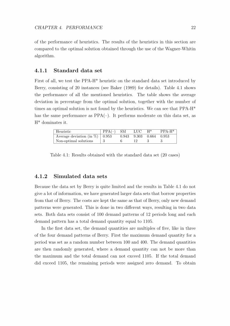
4.1.1 Standard data set

First of all, we test the PPA-H* heuristic on the standard data set introduced by

Berry, consisting of 20 instances (see Baker (1989) for details). Table 4.1 shows

the performance of all the mentioned heuristics. The table shows the average

deviation in percentage from the optimal solution, together with the number of

times an optimal solution is not found by the heuristics. We can see that PPA-H*

has the same performance as PPA(–). It performs moderate on this data set, as

H* dominates it.

Heuristic PPA(–) SM LUC H* PPA-H*Average deviation (in %) 0.953 0.943 9.303 0.664 0.953Non-optimal solutions 3 6 12 3 3

Table 4.1: Results obtained with the standard data set (20 cases)

4.1.2 Simulated data sets

Because the data set by Berry is quite limited and the results in Table 4.1 do not

give a lot of information, we have generated larger data sets that borrow properties

from that of Berry. The costs are kept the same as that of Berry, only new demand

patterns were generated. This is done in two different ways, resulting in two data

sets. Both data sets consist of 100 demand patterns of 12 periods long and each

demand pattern has a total demand quantity equal to 1105.

In the first data set, the demand quantities are multiples of five, like in three

of the four demand patterns of Berry. First the maximum demand quantity for a

period was set as a random number between 100 and 400. The demand quantities

are then randomly generated, where a demand quantity can not be more than

the maximum and the total demand can not exceed 1105. If the total demand

did exceed 1105, the remaining periods were assigned zero demand. To obtain


reasonable demand patterns, the patterns had to comply to a couple of criteria.

First, the last period may not contain a demand quantity of more than 400. This

is done to prevent demand patterns that have very low demand quantities in every

period and then have all the remainder in the last period. Second, the last three

periods may not contain nonzero demand in all three periods. This is to prevent

demand patterns that have very high demand quantities in the first few periods,

resulting in the remainder of the periods having zero demand. Also, the average

percentage deviations of the PPA(–) and H* heuristics applied to the demand

pattern have to be different. In this way, the results for PPA-H* will be more

interesting.

In the second data set, demand quantities may be any nonnegative integer

number and will not be restricted to multiples of five anymore. This data set

is generated by first drawing random uniformly distributed numbers (numbers

between 0 and 1) for all periods. These numbers get scaled to the total demand

of 1105, by multiplying the drawn numbers by the quotient of the total demand

and the sum of the drawn numbers and then being round to integer numbers.

Because of the rounding to integer numbers, the demand quantities may not sum

up to 1105 anymore. This is solved by adding or subtracting the difference from

a randomly chosen period. Similar to the first data set, the average percentage

deviations of the PPA(–) and H* heuristics have to be different.

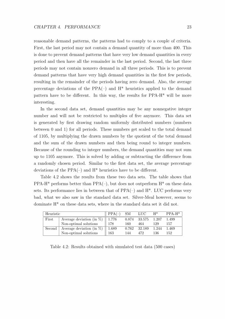
Table 4.2 shows the results from these two data sets. The table shows that

PPA-H* performs better than PPA(–), but does not outperform H* on these data

sets. Its performance lies in between that of PPA(–) and H*. LUC performs very

bad, what we also saw in the standard data set. Silver-Meal however, seems to

dominate H* on these data sets, where in the standard data set it did not.

Heuristic PPA(–) SM LUC H* PPA-H*First Average deviation (in %) 1.776 0.874 33.575 1.207 1.499

Non-optimal solutions 178 160 464 129 157Second Average deviation (in %) 1.689 0.762 32.189 1.244 1.469

Non-optimal solutions 163 144 472 136 152

Table 4.2: Results obtained with simulated test data (500 cases)


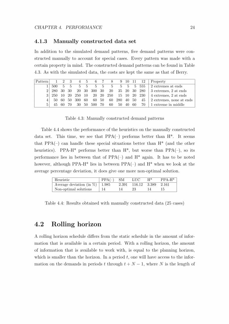
4.1.3 Manually constructed data set

In addition to the simulated demand patterns, five demand patterns were con-

structed manually to account for special cases. Every pattern was made with a

certain property in mind. The constructed demand patterns can be found in Table

4.3. As with the simulated data, the costs are kept the same as that of Berry.

Pattern 1 2 3 4 5 6 7 8 9 10 11 12 Property1 500 5 5 5 5 5 5 5 5 5 5 555 2 extremes at ends2 280 30 30 20 30 300 30 20 35 20 30 280 3 extremes, 2 at ends3 250 10 20 250 10 20 20 250 15 10 20 230 4 extremes, 2 at ends4 50 60 50 300 60 60 50 60 280 40 50 45 2 extremes, none at ends5 45 60 70 30 50 500 70 60 50 40 60 70 1 extreme in middle

Table 4.3: Manually constructed demand patterns

Table 4.4 shows the performance of the heuristics on the manually constructed

data set. This time, we see that PPA(–) performs better than H*. It seems

that PPA(–) can handle these special situations better than H* (and the other

heuristics). PPA-H* performs better than H*, but worse than PPA(–), so its

performance lies in between that of PPA(–) and H* again. It has to be noted

however, although PPA-H* lies in between PPA(–) and H* when we look at the

average percentage deviation, it does give one more non-optimal solution.

Heuristic PPA(–) SM LUC H* PPA-H*Average deviation (in %) 1.985 2.391 116.12 3.389 2.161Non-optimal solutions 14 14 23 14 15

Table 4.4: Results obtained with manually constructed data (25 cases)

4.2 Rolling horizon

A rolling horizon schedule differs from the static schedule in the amount of infor-

mation that is available in a certain period. With a rolling horizon, the amount

of information that is available to work with, is equal to the planning horizon,

which is smaller than the horizon. In a period t, one will have access to the infor-

mation on the demands in periods t through t + N − 1, where N is the length of


the planning horizon. Only this information can be used to decide when the next

replenishment has to take place. This also means no order is permitted to span

a length of time longer than the planning horizon, since there will be not enough

information to decide that.

In practice, contrary to the static schedule, a rolling horizon schedule is used

frequently. This is because in reality one also only knows the demand quantities

for the upcoming few periods in the form of orders placed or forecasts from models.

Because of this, there is also no need for the information when a demand pattern

will end, since future demands may be added indefinitely. This will be no problem

for the rolling horizon schedule.

The data set for the rolling horizon schedule was generated in a similar way as

the data generation of Simpson (2001). Three sets of 300 period patterns, with 10

replications each, were generated and used in the simulations. The generation of

all 30 patterns started with generating 300 normally distributed random variates

for each pattern, where the negative variates were changed to zero. The three sets

represent three levels of demand variability and non-zero demand requirement

frequency. In all three sets, the standard deviation is equal to 1000 (Simpson

(2001) reports a standard deviation of 100, but this actually has to be 1000).

The different means and associated percentages of zero-demand periods and the

coefficients of variation of the generated data set can be found in Table 4.5. The

same costs as stated in Simpson (2001) were used. The per unit, per period

holding cost is equal to 1.0 and the order cost is calculated to be consistent with

the expected order cycle time.

Set Mean Standard deviation % Zero-demand periods Coefficient of variationM50SD10 5000 1000 0 0.20M10SD10 1000 1000 0.16 0.81M5SD10 500 1000 0.31 1.07

Table 4.5: Properties of the data set used in the rolling horizon schedule

The heuristics mentioned in chapter 3 are modified so that no order will span a

length of time longer than the planning horizon. The results from these heuristics

and the Wagner-Whitin heuristic, run with the planning horizon ranging from 4 to

20 periods, are compared to the static schedule benchmark, which are the results


from the Wagner-Whitin algorithm, as well as the rolling horizon benchmark,

which are the results from the constrained Wagner-Whitin.

Table 4.6 reports the performance of the PPA-H* and the other heuristics on

the rolling horizon data set. One can see that the performances of the heuristics

that were also used by Simpson, do not match the performances reported in Simp-

son (2001). This may be caused by the different set of demand patterns, since the

properties of the data set also differ from each other.

H* performs quite bad in the application of a rolling horizon, being next to

last. PPA(–) on the other hand performs rather well, but not as good as the Silver-

Meal or Wagner-Whitin heuristics. As expected, the performance of PPA-H* is

yet again in between that of the PPA(–) and H* heuristics. Although this time,

its performance is very close to that of PPA(–). So PPA-H* performs quite well,

but is still not able to dominate both PPA(–) and H*. Its performance stays in

between that of PPA(–) and H* all the time.

Heuristic Average deviation with respect Average deviation with respectto 300 period benchmark (%) to rolling horizon benchmark (%)

WW 4.2 (3.5) 3.1 (1.9)PPA(–) 6.3 5.2SM 5.6 (6.2) 4.5 (4.6)LUC 13.2 (12.8) 12.2 (11.2)H* 8.7 7.6PPA-H* 6.3 5.3

Table 4.6: Average deviations in a rolling horizon schedule (3060 cases) with resultsfrom Simpson in brackets where applicable

4.3 Variations on PPA-H*

To see whether we can obtain better results with PPA-H*, the criterion for starting

a new order will be altered. Because of the nature of the criterion, this can be

easily done by scaling the measurement values. This modifies expression (3.12)

into

m ·%PPAt−1 < n ·%H∗t−1 and m ·%PPAt ≥ n ·%H∗

t (4.1)

where m, n = {0.1, 0.2, . . . , 1}.


If we change m, while keeping n = 1, it will result in a bias towards the H*

heuristic, since %PPAt loses significance in the criterion. The smaller the m, the

more PPA-H* will act like H*. If m = 0, PPA-H* will perform the same as H* (not

exactly the same though, since PPA-H* will have a strict greater than criterion,

opposed to that of H*, which has a greater or equal criterion). The opposite is also

true, if we keep m = 1 while changing n, it will result in a bias towards PPA(–).

If n = 0, PPA-H* will perform exactly the same as PPA(–).

4.3.1 In the static schedule

First the variations will be tested in the static schedule. The first simulated data

set and the manually constructed data set are used. Table 4.7 shows the perfor-

mance of the variations in the static schedule. It seems there is no variation for

which the performance is the best in both data sets. In the simulated data set,

H* dominates PPA(–) and therefore it is best to keep n = 1 and change m. In the

manually constructed data set however, PPA(–) dominates H*, which means it is

better to keep m = 1 and change n to get a better performance.

Although it seems the performance is quite monotone as m gets larger, and

eventually n gets smaller, there are some exceptions. One of the more interesting

ones is in the simulated data set, when m = 0.1, n = 1. This variation performs

better than H* if we focus on the average deviation. Although, if we look at the

number of non-optimal solutions, it does not perform better. In the manually con-

structed data set, the variations with m = 0.3 and m = 0.4 stand out. While the

other variations with a small m perform worse than PPA-H*, these two variations

actually perform better than PPA-H* and even PPA(–) with regard to the number

of non-optimal solutions and come close to the performance of PPA-H* with re-

gard to the average percentage deviation. However, since this is such a small data

set, this could just be a lucky shot. It seems there is no variation which performs

better overall than the standard PPA-H* in the static schedule.

4.3.2 In the rolling horizon schedule

The variations are also tested on the rolling horizon schedule. Table 4.8 reports

the results of the variations in the rolling horizon schedule. Again the performance


Variation Simulated data set Manually constructed data setm n Avg dev (in %) Non-opt sol Avg dev (in %) Non-opt solH* 1.207 129 3.389 140.1 1 1.189 132 2.868 150.2 1 1.212 138 2.590 150.3 1 1.294 146 2.171 130.4 1 1.385 151 2.171 130.5 1 1.479 156 2.633 150.6 1 1.451 154 2.633 150.7 1 1.457 155 2.633 150.8 1 1.471 158 2.161 150.9 1 1.471 158 2.161 15PPA-H* 1.499 157 2.161 151 0.9 1.481 156 2.161 151 0.8 1.501 157 2.161 151 0.7 1.507 158 2.161 151 0.6 1.579 160 2.419 161 0.5 1.610 168 2.196 151 0.4 1.610 168 2.196 151 0.3 1.628 170 2.196 151 0.2 1.730 173 2.196 151 0.1 1.743 175 2.196 15PPA(–) 1.776 178 1.985 14

Table 4.7: Average deviations and numbers of non-optimal solutions from varia-tions of the PPA-H* heuristic in a static schedule

is quite monotone. PPA(–) dominates H*, thus performance gets better when m

is larger and n is smaller. Although, because of the performance of PPA-H* being

very close to that of PPA(–), there is almost no change in performance when m = 1

and n is changed. There is no variation which stands out from the rest.


Variation Average deviation with respect Average deviation with respectm n to 300 period benchmark (%) to rolling horizon benchmark (%)H* 8.667 7.6120.1 1 7.611 6.5540.2 1 7.227 6.1710.3 1 6.939 5.8820.4 1 6.782 5.7250.5 1 6.683 5.6260.6 1 6.527 5.4700.7 1 6.409 5.3500.8 1 6.370 5.3100.9 1 6.336 5.276PPA-H* 6.340 5.2801 0.9 6.323 5.2621 0.8 6.327 5.2661 0.7 6.323 5.2631 0.6 6.315 5.2561 0.5 6.349 5.2921 0.4 6.349 5.2931 0.3 6.298 5.2421 0.2 6.309 5.2531 0.1 6.353 5.298PPA(–) 6.286 5.230

Table 4.8: Average deviations from variations of the PPA-H* heuristic in a rollinghorizon schedule (3060 cases)

Chapter 5

Conclusion and future research

In this report we studied the performance of a new heuristic which was made

by combining two heuristics. The results in both the static as the rolling hori-

zon schedule show that PPA-H* is a moderate performing heuristic. It does not

perform better than both PPA(–) and H* in any setting. However, it is a fairly

robust heuristic. In some data sets H* performs a lot better than PPA(–), while in

other data sets the opposite happens. Because the performance of PPA-H* lies in

between that of PPA(–) and H* most of the time, it will perform moderate most

of the time. It will not perform very well every time, nor will it perform very bad.

If we look at the results, it seems PPA(–) performs better than H* when there

is a lot of variation in the demand quantities, like with the manually constructed

data and rolling horizon schedule. When the variation in demand quantities is

low, like with the standard data set and simulated data, H* seems to perform

better than PPA(–). When one has a data set with very diverse demand patterns,

PPA-H* might be a good choice.

As we can see from the results from the variations, scaling one of the measure-

ment values does have an influence on the performance of PPA-H*. However, it

is dependent on the data set whether the scaling will be for the better or worse.

There is no variation that performs better than the standard PPA-H* at all times.

To keep the PPA-H* heuristic robust, it is best to keep the standard form, instead

of applying a variation. Although if one prefers the properties of either PPA(–) or

H* over the other, scale parameters n or m may be altered respectively.

30

CHAPTER 5. CONCLUSION AND FUTURE RESEARCH 31

We conclude this report with some issues for further research. First, a worst

case analysis may be performed. Both PPA(–) and H* have a worst case ratio of

2, but this does not mean PPA-H* will also have a worst case ratio of 2. Fur-

thermore, the initial idea was to construct a heuristic, borrowing the good aspects

of two well-performing heuristics, that would perform better than both the com-

posite heuristics. Unfortunately, we did not achieve this goal with our method of

combining the heuristics. Maybe it is possible to combine the heuristics in such a

way that this goal will be achieved. It may also be profitable to look at combining

other heuristics.

Bibliography

Kenneth R. Baker. Lot-sizing procedures and a standard data set: A reconciliation

of the literature. Working Paper, 243, 1989.

J.J. DeMatteis. The part-period algorithm. IBM Systems Journal, 7(1):30–39,

1968.

E.A. Silver and H.C. Meal. A heuristic for selecting lot size quantities for the case of

a deterministic time-varying rate and discrete opportunities for replenishment.

Production and Inventory Management, 2nd Quarter:64–74, 1973.

Edward Allen Silver, David F. Pyke, and Rein Peterson. Inventory management

and production planning and scheduling, chapter 6. Wiley, New York, 1998.

ISBN 0-471-11947-4.

N.C. Simpson. Questioning the relative virtues of dynamic lot sizing rules. Com-

puters & Operations Research, 28:899–914, 2001.

Wilco Van den Heuvel and Albert P.M. Wagelmans. Worst case analysis for a

general class of on-line lot-sizing heuristics. Operations Research, published

online before print, June 3 2009a.

Wilco Van den Heuvel and Albert P.M. Wagelmans. A holding cost bound for the

economic lot-sizing problem with time-invariant cost parameters. Operations

Research Letters, 37:102–106, 2009b.

H.M. Wagner and T.M. Whitin. Dynamic version of the economic lot size model.

Management Science, 5:89–96, 1958.

32

combining heuristics for the economic lot-sizing problem · abstract this report shows a new...

Documents