a dynamic lot-sizing-based profit maximization discounted
TRANSCRIPT
HAL Id: halshs-01683781https://halshs.archives-ouvertes.fr/halshs-01683781
Submitted on 14 Jan 2018
HAL is a multi-disciplinary open accessarchive for the deposit and dissemination of sci-entific research documents, whether they are pub-lished or not. The documents may come fromteaching and research institutions in France orabroad, or from public or private research centers.
L’archive ouverte pluridisciplinaire HAL, estdestinée au dépôt et à la diffusion de documentsscientifiques de niveau recherche, publiés ou non,émanant des établissements d’enseignement et derecherche français ou étrangers, des laboratoirespublics ou privés.
A dynamic lot-sizing-based profit maximizationdiscounted cash flow model considering working capital
requirement financing cost with infinite productioncapacity
Yuan Bian, David Lemoine, Thomas Yeung, Nathalie Bostel, VincentHovelaque, Jean-Laurent Viviani, Fabrice Gayraud
To cite this version:Yuan Bian, David Lemoine, Thomas Yeung, Nathalie Bostel, Vincent Hovelaque, et al.. A dynamic lot-sizing-based profit maximization discounted cash flow model considering working capital requirementfinancing cost with infinite production capacity. International Journal of Production Economics,Elsevier, 2018, 196, pp.319-332. �10.1016/j.ijpe.2017.12.002�. �halshs-01683781�

MANUSCRIP
T
ACCEPTED
ACCEPTED MANUSCRIPTInternational Journal of Production Economics
Title: A dynamic lot-sizing-based profit maximization discounted cash flow model considering working capital requirement financing cost with infinite production capacity
Authors: YuanBIAN∗, DavidLEMOINE, ThomasG. YEUNG, NathalieBOSTEL , VincentHOVELAQUE%, Jean-laurentVIVIANI%, FabriceGAYRAUD
Affiliations:
a : LS2N, UMR CNRS 6004, IMT Altantique, 4, Rue Alfred Kastler, B.P. 20722, 44307 Nantes, France
b : LS2N, UMR CNRS 6004, University of Nantes, 58 rue Michel Ange, B.P. 420, 44606 Saint-Nazaire, France
c : CREM, UMR CNRS 6211, IGR-IAE of Rennes, University of Rennes 1, 11 rue Jean Macé, 35708 Rennes, France
* : Corresponding author
Yuan BIAN
LS2N, UMR CNRS 6004,
IMT Altantique,
4, Rue Alfred Kastler, B.P. 20722, 44307 Nantes Cedex 3, France,
Phone : (0033)251858335
E-mail : [email protected]

MANUSCRIP
T
ACCEPTED
ACCEPTED MANUSCRIPT
A dynamic lot-sizing-based profit maximization discounted cashflow model considering working capital requirement financing
cost with infinite production capacity
Abstract
In times of crisis, companies need free cash flow to efficiently react against all uncertainty to
ensure solvency. However, classical dynamic lot-sizing models only consider the physical flow of
goods. In this paper, we introduce a first link between dynamic lot-sizing and the financial aspects
of working capital requirements (WCR). We propose a new generic WCR model which allows
us to evaluate the company’s financial situation throughout the planning horizon. Moreover, a
dynamic lot-sizing-based, discounted cash flow model is established for single-site, single-level,
single-product and infinite capacity cases. It is shown that the zero-inventory ordering property
holds for this case and thus a polynomial-time algorithm may be utilized. Numerical tests are
presented in order to show the relevance of our approach compared with the traditional dynamic
lot-sizing model.
Keywords: profit maximization; dynamic lot-sizing; working capital requirement; discounted
cash flow; delays in payment.
1. Introduction
According to the Ernst & Young annual Working Capital Management (WCM) report of
2012 devoted to the leading 1000 US companies in year 2011, on average, $330 billion dollars
of Net Working Capital (NWC) is unnecessarily immobilized (see in Ernst (2012)). This range
of cash opportunity corresponds to, respectively, between 3% and 6% of their aggregate sales.
Buchmann et al. (2008) also stress that savings on Working capital Requirement (WCR) as a
potential source of cash to fund growth is often neglected by companies. Suboptimal WCM
not only reduces potential gains, it also raises companies’ risk. A company needs to carefullyPreprint submitted to International Journal of Production Economics November 30, 2017
MANUSCRIP
T
ACCEPTED
ACCEPTED MANUSCRIPT
manage its WCR in order to ensure financial liquidity or reduce insolvency risk. Additionally,
optimal WCM can unlock internal capital and provide financial resources to financially constrai-
ned firms. Especially during the last financial crisis, bank loans were extremely difficult to obtain
by companies, especially those in the development phase (see in Wu et al. (2016)). Many com-
panies suffer from lack of credit and insufficient working capital. Small suppliers are forced to
accept unfavorable payment terms from their customers, exacerbating their financial situation.
Moreover, tight or unavailable bank credit reduces the working capital level of these companies.
As a result, some companies must suspend their operations which can disrupt the whole supply
chain as reported in Benito et al. (2010) and Ernst (2010).
In spite of its importance for firm (and more generally the supply chain) performance and
survival, WCM has been neglected by the literature on production planning. More generally, as
stated by Birge (2014), ”Operations management models typically only consider the level and
organization of a firms transformation activities without considering the financial implications
of those activities”. The separation of the operational decision (minimizing operational costs
or maximizing operational profits) and financial decision (minimizing financial costs or maxi-
mizing financial profit) was theoretically grounded on the famous Modigliani and Miller (1958)
theorem and practically by the functional organization of companies. However, in recent years,
the literature on operations and supply chain management, following the original work of Babich
and Sobel (2004), became aware of the fact that financing and operational problems are imbrica-
ted and that optimizing the two dimensions jointly could improve the global performance of the
company as shown in Chen et al. (2014). A recent review of this literature based on a risk mana-
gement framework has been proposed by Zhao and Huchzermeier (2015). Nevertheless, in the
production planning field, the majority of models typically ignore the financial consequences of
production planning decisions. In an attempt to fill this gap, the aim of the paper is to explicitly
introduce the financial dimension in a tactical production planning model.
Traditionally, tactical production planning aims at determining the production quantity for
each period of the planning horizon. It is often known for its strong influence in terms of custo-
mer service quality and production related operation costs. Two main classes of models distin-
2

MANUSCRIP
T
ACCEPTED
ACCEPTED MANUSCRIPT
guish the problem based on continuous/discrete time considerations: for example, with infinite
capacity, the Economic Order Quantity (EOQ) model of Harris (1913) for constant demand over
continuous time and the Uncapacitated Lot-Sizing model (ULS) of Wagner and Whitin (1958)
for time-varying demand over discrete time. Readers can refer to the literature review of Brahimi
et al. (2017) for single item cases and of Comelli et al. (2006) for model classification. However,
production planning is determined following the well-known Manufacturing Resource Planning
(MRP II) logic for a medium-term objective. As indicated by Helber (1998), this decision does
not reflect difference in Net Present Value (NPV) of cash flow due to planned operations in real
world market system. Moreover, financial aspects are rarely considered in dynamic lot-sizing
literature.
In order to better take into account the financial dimension in a production planning context,
we first replace the total operational cost minimization objective by the overall financial objective
of the firm, which is the wealth maximization objective. The total wealth represents the sum
of the net present values of all future cash flows. This remains the main stream objective in
corporate finance as stated in Jensen (2001). The importance of this objective has also been
recognized in the production planning literature (see Serrano et al. (2017)).
Second, we introduce a joint management of both physical and financial flows within a dis-
counted cash flow-based dynamic LSP model. We consider both classical operational costs (e.g.,
purchasing, setup, production) and financial costs. More specifically, financial costs are gene-
rated by the need to finance the Working Capital Requirement(WCR) induced by operational
decisions. In practice, the WCR is known as a key indicator to monitor and control a company’s
financial situation. The WCR is mainly caused by the timing mismatch between the cash inflows
and the cash outflows associated with the total production and commercial cycle as presented
in Theodore Farris and Hutchison (2002). According to the cash conversion cycle methodology
proposed by these authors, the free cash flow level can be approximately measured as the diffe-
rence between the working capital and WCR. As a consequence, a lower operating WCR gives
the company better liquidity and helps to ensure solvency. By this direct link with cash flow,
the WCR increasingly draws the attention of finance departments in a financial crisis context.
3
MANUSCRIP
T
ACCEPTED
ACCEPTED MANUSCRIPT
By introducing the financing cost of the WCR, the traditional trade-off between set-up costs and
inventory costs is therefore modified. If the company orders lots of bigger size, it will not only
increase inventory costs, but also the WCR, leading to higher financial costs.
The main contributions of this paper are the following:
• First, we propose a WCR model adapted to the production planning context. This allows
us to precisely measure the WCR during the planning horizon;
• Second, we demonstrate that the Zero-Inventory-Ordering property remains valid in this
problem. This ensures a strong structural property of the optimal solution and its exact
resolution in polynomial time. Moreover, it shows no additional computational complexity
by introducing the financial cost into the optimization objective;
• Finally, we show significant differences between optimal production planning obtained by
the classic dynamic lot-sizing model and our proposed model.
This remainder of this paper is organized as follows: In Section 2, related works that consider
a financial aspect in tactical production planning and profit maximization models are reviewed.
In Section 3, we propose a generic model of operating WCR in a tactical production planning
context. We then develop a profit maximization model based on a classic dynamic LSP model by
using the OWCR model for the single-product with infinite capacity case. In Section 4, the Zero-
Inventory-Ordering property is proven and a dynamic programming algorithm is consequently
established. In Section 5, we analyze the differences of both the optimal production planning of
the proposed model and the classical dynamic lot-sizing model in terms of production planning.
We end with a short conclusion and show insights for further research.
2. Literature Review
The management of financial flow is an important part of supply chain management (SCM)
as shown in Cooper et al. (1997) and Vidal and Goetschalckx (2001). However, formal analytical
models have only recently become available in Raghavan and Mishra (2011) and Liu and Cruz
(2012). They aim to understand how the planning, management and control of financial flows in4
MANUSCRIP
T
ACCEPTED
ACCEPTED MANUSCRIPT
supply chains affect the chain profitability. In addition, inventory management models have been
reformulated to take into account financial considerations such as trade credit, delay in payment
or financial risks, as in Aggarwal and Jaggi (1995), Berling and Rosling (2005) and Gupta and
Wang (2009). Moreover, Protopappa-Sieke and Seifert (2010) elaborate on the interest of con-
sidering decision making in both operational and financial levels for the physical and financial
supply chain by determining the optimal purchase order quantity. In addition, Zeballos et al.
(2013) explain the evolution of the Modigliani and Miller theorem in the field of inventory ma-
nagement and propose a single-product, finite horizon model that considers the financial aspects
of working capital constraints, payment delays and short-term debts. These studies highlight the
fact that in supply chain management, physical flow and financial information must be managed
jointly.
We consider WCR in tactical production planning because working capital management
(WCM) has been identified as an important indicator for measuring supply chain performance
by Timme and Williams-Timme (2000). The influence of WCM on a company’s performance
and profitability have been confirmed by several national studies by Ding et al. (2013), Enqvist
et al. (2014), Vahid et al. (2012) and Bei and Wijewardana (2012) and in different industrial sec-
tors, e.g., the restaurant and automotive industry in Lind et al. (2012) and Mun and Jang (2015),
respectively. In addition, Kieschnick et al. (2013) report that for the average firm the incremen-
tal dollar invested in net working capital is worth less than the incremental dollar held in cash.
Since free cash flow level is the difference between working capital level and the WCR level, if
the working capital remains constant, the minimum level of WCR represents the maximum level
of free cash flow. According to the accounting formula of WCR in finance, delays in payment
both from the customer and to the supplier significantly influence the level of WCR. In practice,
such a delay is often accepted by the supplier to the customer in the form of trade credit.
Furthermore, as a financial consideration, the time value of money has drawn significant at-
tention for building cash flow analysis models, namely the Discounted Cash Flow (DCF) model.
The Net Present Value (NPV) metric is adopted to measure the present value of future cash flow
in order to calculate the profitability of a projected investment or project. Since the work of Trippi
5
MANUSCRIP
T
ACCEPTED
ACCEPTED MANUSCRIPT
and Lewin (1974), the time value of money aspect has been largely addressed based on the classic
EOQ model. More related works are discussed in reviews of Taleizadeh and Nematollahi (2014)
and Martınez-Costa et al. (2014). In the single-site dynamic lot-sizing literature, the DCF mo-
dels can also be found since the work of Helber (1998) in various industry contexts. The author
develops a cash-flow oriented multi-level lot-sizing model in MRP II (Manufacturing Resource
Planning) system. Recently, Lim et al. (2013) establish a mathematical model in order to obtain
the optimal product portfolio and the processing route of an integrated, resource-efficient rice
mill complex with a profit maximization objective. Mitra et al. (2014) propose a Mixed Integer
Linear Programming (MILP) formulation that combines the operational and strategic decisions
for continuous power-intensive processes under time-sensitive electricity prices.
In addition, the aspect of working capital has often been considered in term of capital or
budget constraints in inventory management literature. Recently, Wang et al. (2007a) address
the acquisition and allocation of LCD (Liquid-Crystal Display) manufacturing industries which
requires a high amount of capital investments. In this problem, the authors included not only con-
straints of operational aspect, e.g., resource capacity constraints and backorder, but also financial
aspects of finite budget and the time value of capital and asset. Wang et al. (2007b) propose a
mathematical programming model for a generalized resource portfolio problem in a context of
the semiconductor testing industry considering the financial resource constraints and the time
value of capital. Chao et al. (2008) study the influence of loan limits on the operation decision
in the EOQ context. Thomas and Bollapragada (2010) develop an analytical decision tool based
on a capacity planning model to estimate product costs and demands in order to maximize the
NPV of profit for General Electric. Lusa et al. (2012) develop a MILP formulation of an integral
planning model with a maximum level of working capital constraints.
In this paper, therefore, we are interested in proposing a new generic operating WCR (OWCR)
model in a tactical planning framework for a dynamic LSP model. For this reason, we propose
a DCF-based profit maximization model considering the upstream and downstream payment de-
lays and the financing cost of OWCR. A comparison between the aforementioned single-site
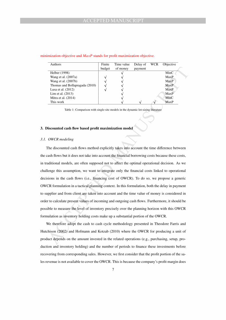
dynamic lot-sizing-based models and our research is presented in Table 1. MinC stands for cost
6
MANUSCRIP
T
ACCEPTED
ACCEPTED MANUSCRIPT
minimization objective and MaxP stands for profit maximization objective.
Authors Finite Time value Delay of WCR Objectivebudget of money payment
Helber (1998)√
MinCWang et al. (2007a)
√ √MaxP
Wang et al. (2007b)√ √
MaxPThomas and Bollapragada (2010)
√ √MaxP
Lusa et al. (2012)√ √
MaxPLim et al. (2013)
√MaxP
Mitra et al. (2014)√
MinCThis work
√ √ √MaxP
Table 1: Comparison with single-site models in the dynamic lot-sizing literature
3. Discounted cash flow based profit maximization model
3.1. OWCR modeling
The discounted cash flows method explicitly takes into account the time difference between
the cash flows but it does not take into account the financial borrowing costs because these costs,
in traditional models, are often supposed not to affect the optimal operational decision. As we
challenge this assumption, we want to integrate only the financial costs linked to operational
decisions in the cash flows (i.e., financing cost of OWCR). To do so, we propose a generic
OWCR formulation in a tactical planning context. In this formulation, both the delay in payment
to supplier and from client are taken into account and the time value of money is considered in
order to calculate present values of incoming and outgoing cash flows. Furthermore, it should be
possible to measure the level of inventory precisely over the planning horizon with this OWCR
formulation as inventory holding costs make up a substantial portion of the OWCR.
We therefore adopt the cash to cash cycle methodology presented in Theodore Farris and
Hutchison (2002) and Hofmann and Kotzab (2010) where the OWCR for producing a unit of
product depends on the amount invested in the related operations (e.g., purchasing, setup, pro-
duction and inventory holding) and the number of periods to finance these investments before
recovering from corresponding sales. However, we first consider that the profit portion of the sa-
les revenue is not available to cover the OWCR. This is because the company’s profit margin does
7

MANUSCRIP
T
ACCEPTED
ACCEPTED MANUSCRIPT
not correspond to the definition of working capital requirement since it has never been required.
Furthermore, this assumption supposes that the company does not prioritize its profit allocation
to WCR financing. Profit can be allocated to any of a number of objectives for the firm including
debt reduction, internal or external investment, or dividend payments. Our model is a partial
model of the company and we do not assume that allocation of profit to WCR financing rather
than to other objectives (e.g., new investments) is optimal. Moreover, following the Modigliani
Miller Theorem, a company should not allocate a specific financial resource (in this case, profit)
to a specific object (in this case, WCR financing). In consequence, we adopt the scheme that the
WCR generated by producing a product is only effectively recovered when that product is sold.
This assumption complicates the calculation of the financing duration of setup costs because
it is paid in its entirety at a single point in time for the entire production lot. Thus, we must
progressively and uniformly recover the setup cost from the sales revenue of all products in the
same production lot. These products therefore share the fixed setup cost equally as the amount
invested and the number of periods to finance is the time difference between the period when the
setup occurs and the period of sale of each product.
3.2. Assumptions
Since this model is built in the context of the ULS (Uncapacitated Lot-Sizing) problem, the
OWCR formulation and the corresponding profit maximization model proposed in this paper are
based on the following assumptions:
• Production:
– No replenishment and production delays as they are negligible compared with period
duration;
– Demand should be met on time (no backlogging);
– Only inventory of final product is considered;
– Initial and final stock are defined as zero;
– One unit of finished product is manufactured using one unit of raw material.
8

MANUSCRIP
T
ACCEPTED
ACCEPTED MANUSCRIPT
• Financial:
– All logistic and financial costs are paid at the beginning of periods;
– The profit from selling products is not be used for financing the OWCR;
– The fixed setup cost of a given lot is progressively and uniformly recovered over the
different periods during which the products of the corresponding lot are sold;
– All holding costs paid for a product for all periods it remains in inventory are not
recovered until it’s sale.
3.3. Physical and financial flow illustration
With the aforementioned assumptions, we express in detail in Figure 1, the physical and
financial flows generated by a production in period 1 for the demand of period 3. In this case, we
assume the delays in payment from client and to supplier are both one period.
• Physical flows are presented in the top block. They are generated by decisions made in the
operating cycle, such as purchase, production, inventory holding and delivery. Therefore,
the physical flows link all decisions in the graphic with the single line arrow.
• The financial flows are displayed in the bottom block. First, the logistic costs are immedi-
ately generated by the physical activities presented by small squares in the financial block.
Meanwhile, the WCR financing costs are also to be paid from the same period of corre-
sponding logistic costs until the reception of revenue. These financial costs are presented
with the double line arrow.
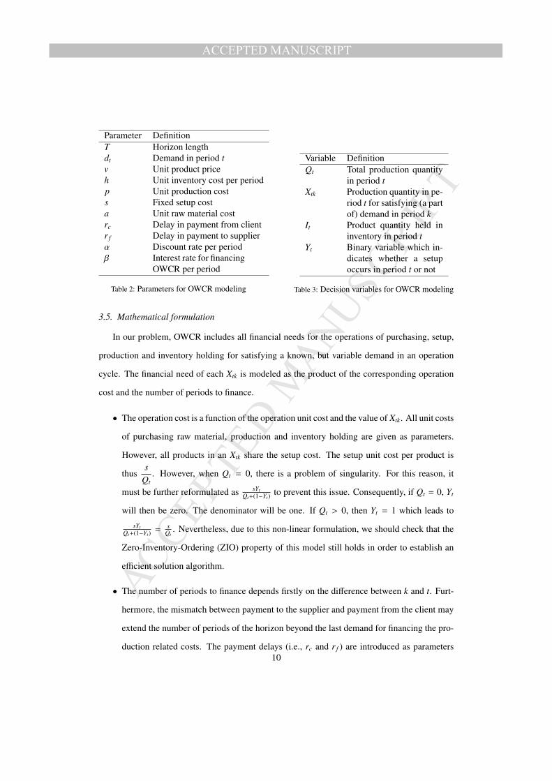
3.4. Parameters and decision variables
In this model, parameters and decision variables are adopted for the single-site, single-level,
single-product with infinite capacity case. Their notations are given in Tables 2 and 3 respecti-
vely. We assume that these parameters are all nonnegative. We choose the decision variables
of the FAL (FAcility Location) formulation of the ULS. These disaggregated variables allow
us to measure the exact amount of incoming and outgoing payments for all production related
operations considered for calculating the OWCR.9
MANUSCRIP
T
ACCEPTED
ACCEPTED MANUSCRIPT
Parameter DefinitionT Horizon lengthdt Demand in period tv Unit product priceh Unit inventory cost per periodp Unit production costs Fixed setup costa Unit raw material costrc Delay in payment from clientr f Delay in payment to supplierα Discount rate per periodβ Interest rate for financing
OWCR per period
Table 2: Parameters for OWCR modeling
Variable DefinitionQt Total production quantity
in period tXtk Production quantity in pe-
riod t for satisfying (a partof) demand in period k
It Product quantity held ininventory in period t
Yt Binary variable which in-dicates whether a setupoccurs in period t or not
Table 3: Decision variables for OWCR modeling
3.5. Mathematical formulation
In our problem, OWCR includes all financial needs for the operations of purchasing, setup,
production and inventory holding for satisfying a known, but variable demand in an operation
cycle. The financial need of each Xtk is modeled as the product of the corresponding operation
cost and the number of periods to finance.
• The operation cost is a function of the operation unit cost and the value of Xtk. All unit costs
of purchasing raw material, production and inventory holding are given as parameters.
However, all products in an Xtk share the setup cost. The setup unit cost per product is
thuss
Qt. However, when Qt = 0, there is a problem of singularity. For this reason, it
must be further reformulated as sYtQt+(1−Yt)
to prevent this issue. Consequently, if Qt = 0, Yt
will then be zero. The denominator will be one. If Qt > 0, then Yt = 1 which leads to
sYtQt+(1−Yt)
= sQt
. Nevertheless, due to this non-linear formulation, we should check that the
Zero-Inventory-Ordering (ZIO) property of this model still holds in order to establish an
efficient solution algorithm.
• The number of periods to finance depends firstly on the difference between k and t. Furt-
hermore, the mismatch between payment to the supplier and payment from the client may
extend the number of periods of the horizon beyond the last demand for financing the pro-
duction related costs. The payment delays (i.e., rc and r f ) are introduced as parameters10

MANUSCRIP
T
ACCEPTED
ACCEPTED MANUSCRIPT
in order to quantify this mismatch. Using these parameters, we define the start period to
finance the corresponding production related costs as well as the end period, as presented
in Table 4.
Operation cost Periods to finance
Operations Unit cost × Quantity from( the period ofoutgoing payment
)until
( the period ofincoming payment
)Purchasing a × Xtk from (t + r f ) until (k + rc − 1)
SetupsYt
Qt + (1 − Yt)× Xtk from t until (k + rc − 1)
Production p × Xtk from t until (k + rc − 1)Inventory holding h × Xtk Financing periods (FP)
Table 4: Formulation of OWCR components
Although the costs of purchasing, set-up and production are all one-time payments for each
production lot, the inventory holding cost is paid regularly in all periods where the stock is held
in inventory. For this reason, there is a cumulative effect of financing the inventory holding costs.
Assuming that a production lot covers all demands from period t to period k means that the
production occurs in period t at the latest. A unit of product of the demand in period k will be
sold in period k and the client’s payment will arrive in period k + rc. The inventory holding cost
for this item should be paid consequently from period t until period k − 1 (noted as ”OWCRinv
series”). The first of these payments occurs in period t and must be financed until period k+rc−1
(before the arrival of the client’s payment, so a total of k + rc − t periods must financed). The
second is paid in period t + 1 until the same period of k + rc − 1 (in total, k + rc − (t + 1) periods
to finance.), etc. Consequently, for each Xtk, the financing period is1 + (k − t)
2(k − t) + rc(k − t)
periods including all periods to finance before and after the demand delivery.
Following this formulation of OWCR, the OWCR at period t, written as Ot, can be expressed
in the following:
Ot = at−r f∑j=1
T∑l=t−rc+1
X j,l + pt∑
j=1
T∑l=t−rc+1
X j,l + st∑
j=1
T∑l=t−rc+1
Y j
Q j + (1 − Y j)X j,l
+ht∑
j=1
T∑l=t−rc+1
X j,l · (min {l, t + 1} − j) (1)
11

MANUSCRIP
T
ACCEPTED
ACCEPTED MANUSCRIPT
The formulationt−r f∑j=1
T∑l=t−rc−1
X j,l represents all products whose production related operations
still have to be financed at period t considering the payment delays. Especially for measuring
the total amount of inventory holding cost to finance at period t, we need to count the number
of completed payments in the OWCRinv series until period t for each X j,l. However, we must
consider whether or not we have sold the products of X j,l before reception of the client’s payment
(in other words, whether or not Xtk is still in inventory). min {l, t + 1} − j precisely represents the
total number of all payments for these two possible cases. The difference between these two
cases as presented in formulation (1) is:
• If we have sold Xtk at period t (i.e. l ≤ t < l + rc), then the total amount to finance for
inventory holding will not change during the periods before arrival of the client’s payment.
This is because we no longer need to pay the inventory holding cost for Xtk in these periods.
Thus, no additional inventory hold cost must be financed which means the total amount is
a function of l − j.
• On the contrary, if the Xtk is still in inventory (i.e. j ≤ t < l), then the total amount of
inventory holding costs to finance depends on t + 1 − j.
This formulation of OWCR allows us to follow the variation of OWCR over time in the planning
horizon. It will be used in the following section for calculating the financing cost of OWCR.
3.6. Objective function
The objective of this problem is to maximize the NPV of the profit (denoted by Pro f it)
by satisfying variable demand. To simplify the problem, the NPV of profit is defined as the
difference between the NPV of revenue and the NPV of expenses. In our model, the revenue
per period is a function of constant unit sales prices and demand quantity. The expenses include
the production costs and the OWCR financing costs. The production cost is the sum of the costs
for raw material purchasing, machine setup, production and inventory holding. The OWCR
financing cost depends on the interest rate and the OWCR for satisfying all the demand on-time.
Considering the payment delays, the planning horizon must be extended to the period when
12

MANUSCRIP
T
ACCEPTED
ACCEPTED MANUSCRIPT
the last incoming or outgoing cash flow occurred. Mathematically, this accounting horizon is
presented as T + max {r f , rc}. For simplification purposes, T denotes the accounting horizon in
this paper. Since the time value of money is considered in this model, both cash inflow (i.e.,
revenues) and outflow (i.e., expenses) are presented in NPV as follows:
• NPV of revenue in period t, Rt: due to the delay of the client’s payment, we only receive
the client’s payment for the demand of period t − rc in period t. Thus, Rt = 1(1+α)t vDt−rc .
• NPV of production cost in period t, LCt: all expenses of production related operations
must be paid immediately when they occur except for the purchasing cost which can be
delayed r f periods according to the supplier agreement. Therefore, LCt = 1(1+α)t (aQt−r f +
pQt + sYt + hIt) with Qt =T∑
k=tXtk and It =
t∑l=1
T∑k=t+1
Xlk.
• NPV of OWCR financing cost in period t, FCt: The OWCR financing cost depends only
on the interest rate per period and the amount of financial need (i.e., Ot) to cover in period
t. FCt = 1(1+α)t βOt.
By summing over all periods of the accounting horizon, the objective function is formulated
as follows:
Pro f it =T∑
t=1(Rt − LCt − FCt)
3.7. ULS P(WCR) model
A mixed-integer model of the profit maximization problem, ULS P(WCR), is formulated as
follows:
Max Pro f it (1.1)
s.t. Qt =∑T
k=t Xtk ∀t (1.2)
dkYt − Xtk ≥ 0 ∀t, k (1.3)
Yt − Qt ≤ 0 ∀t (1.4)∑kt=1 Xtk = dk ∀k (1.5)
Xtk ≥ 0,Yt ∈ {0, 1} ∀t, k (1.6)13

MANUSCRIP
T
ACCEPTED
ACCEPTED MANUSCRIPT
The objective function is to maximize the NPV of total profit. The constraints are similar to
those of the FAL formulation of the ULS. Constraints (1.2) indicate that Qt is the total quantity
of production that occurs in period t. Constraints (1.3) ensure that a setup is executed before
production. Constraints (1.4) prevent a setup from occurring in a period with no production.
Finally, constraints (1.5) ensure that all demands are satisfied.
4. Solution method
In order to solve the ULS P(WCR) problem efficiently, we propose an algorithm which avoids
the difficulty of the non-linear formulation of the setup cost in the OWCR calculation. This algo-
rithm is similar to the algorithm which is based on the Zero-Inventory-Ordering (ZIO) property
established for the ULS problem with infinite capacity by Wagner and Whitin (1958).
4.1. Zero-Inventory-Ordering property
In a ZIO-type planning, production is only planned when no products remain in the inven-
tory. We demonstrate that an optimal solution can always be found within all possible plans that
respect the ZIO property. Moreover, since only ZIO type plans need to be investigated to find
the optimal solution, the number of feasible solutions to investigate is significantly reduced. The
ZIO property can be expressed as follows:
Theorem: There exists an optimal production plan in which It−1 × Qt = 0 for all t (where It
is the inventory at the end of the period t) in ULS P(BFR) problem.
The proof is presented in Appendix A. The main idea is to demonstrate that we can always
improve the objective value by eliminating violation(s) of the property by transforming a pro-
duction plan which does not comply with the ZIO property to a ZIO-type plan. Eventually, we
can prove the ZIO-type production program provides the optimal objective value.
4.2. Algorithm description
Since the demand, the delay in payment from the customers, and the discounted rate are
all given, the NPV of revenue is fixed for each instance. Thus, we only need to minimize the
NPV of all costs. Then, like the classical shortest path problem, the ULS P(BFR) problem is14

MANUSCRIP
T
ACCEPTED
ACCEPTED MANUSCRIPT
formulated with an acyclic oriented graph G = {V, E} (see Figure 2). The nodes Vt represent
the T periods in the planning horizon including a dummy node at the end (node 6 in Figure
2). Moreover, determining the production quantity benefits from the ZIO property which means
that the production quantity can only be the sum of demands in the following periods. We thus
avoid the difficulty caused by the nonlinear formulation of setup cost to finance. Consequently,
an arc Etk denotes a production planned in period t for all demands between periods t and k −
1. With this concept and the ZIO property, we determine the precise quantity and period of a
production as well as the delivery periods. We are thus able to deduce the period of client’s
payment for financial cost calculation. Finding a shortest path therefore allows us to obtain the
optimal production program with the minimum total NPV of all costs generated. Furthermore,
with the dummy node, we are able to express all types of production lots in this acyclic graph
including ”make-to-order” type production.
In the objective function of ULS P(WCR), an aggregate OWCR formulation is given. However,
a Xtk-based formulation of NPV of OWCR is required for arc value calculations. In the former
formulation, the OWCR of an operation is the product of the corresponding unit cost, Xtk, and the
number of periods to finance. Considering the NPV of OWCR, the discount rates are different
(decreasing) during the periods to finance. Thereby, the discounted OWCR depends on the period
where the payment occurred. WCRpurtk , WCRset
tk , WCRprodtk and WCRInv
tk respectively stand for
the OWCR generated by operations of purchasing, set-up, production and inventory holding
for producing the Xtk. For example, in purchasing raw material for the production of Xtk, the
payment to supplier is made in period t + r f and the client’s payment is received in period k + rc.
Therefore, the corresponding discounted OWCR represents all financial needs to be covered
between t + r f and k + rc. However, we are not able to ensure the timing order between the
payment to supplier and the collection of clients payment. For this reason, we consider that we
continue to finance the payment to the supplier until the end of the planning horizon as well
as the payment from customer. The mathematical formulation can be written as WCRpurtk =
aXtk
T∑j=t+r f
1(1 + α) j −
T∑j=k+rc
1(1 + α) j
. (By considering the financing cost of OWCR, the horizon
is extended because some payments may be received from the client or sent to the supplier after
15

MANUSCRIP
T
ACCEPTED
ACCEPTED MANUSCRIPT
the last period of the planning horizon).
This formula allows us to correctly cover the two cases whether the payment to supplier or
client’s payment occurs first. In the first case, a negative OWCR in purchasing will be obtained
which can be considered as an additional refund for the OWCR of other operations. In the second
case, WCRpurtk is a positive financial need to finance.
Following the same concept, the OWCR in other operations can be formulated as
• WCRsettk =
sYt
Qt + (1 − Yt)Xtk
k+rc−1∑j=t
1(1 + α) j ,
• WCRprodtk = pXtk
k+rc−1∑j=t
1(1 + α) j ,
• and WCRInvtk = hXtk
k−1∑l=t
k+rc−1∑j=l
1(1 + α) j .
For WCR of inventory holding, if k = t (i.e., Xtk is produced for demand in the same period),
then there is no inventory holding cost. Combining all these components, the total OWCR for all
Xtk, denoted as WCRtotal, can be written as follows:
WCRtotal =T∑
t=1
T∑k=1
(WCRpurtk + WCRset
tk + WCRprodtk + WCRInv
tk )
To simplify the NPV formulation, note that a′t = a 1(1+α)t , s′t = s 1
(1+α)t , p′t = p 1(1+α)t and h′t =
h 1(1+α)t . With the ZIO property, the arc values are presented as follows (with LCtk representing
all the production costs):
Etk = LCtk + β
k−1∑l=t
(WCRpur
tk + WCRsettk + WCRprod
tk + WCRInvtk
)= (a′t+r f
+ p′t)k−1∑l=t
dl + s′t +
k−1∑l=t
dl
l−1∑i=t
h′i
+β
k−1∑l=t
dl
T∑
j=t
a′j+r f−
T∑j=l
a′j+rc
+
l+rc−1∑j=t
p′j +
l+rc−1∑j=t
s′jk−1∑i=t
di
+
l−1∑i=t
l+rc−1∑j=i
h′j
(2)
16

MANUSCRIP
T
ACCEPTED
ACCEPTED MANUSCRIPT
The computation of Etk is done in O(T 2). The objective of this algorithm is to find the shortest
path to the last node. To do so, we need to progressively locate the shortest path to other nodes.
We therefore examine all possible paths to each node from all its predecessors through the arc in
between. This can be carried out by the recursive function
Pro f it[t] = minj∈[1,t−1]
{Pro f it[ j] + E jt}
with Pro f it[t] the minimum total cost to finance to satisfy all demands until period t. Thus, a
dynamic programming algorithm is established as presented in Algorithm 1. The complexity of
the algorithm is O(T 4), thus the ULS P(WCR) problem can be solved in polynomial time.
Algorithm 1 Solving ULS P(WCR)
Require: All parameter valuesfor i = 2 to T-1 do
for j = 1 to i − 1 doif Pro f it[i] > Pro f it[ j] + E ji then
Pro f it[i] = Pro f it[ j] + E ji
end ifend for
end for
5. Numerical examples
Through the following numerical tests, we reveal differences between optimal production
plans for profit maximization and costs minimization objectives. These tests illustrate the influ-
ence of considering the financing cost of OWCR on an optimal production program. With the
proven ZIO property, the optimal program of profit maximization problem is calculated and de-
noted as Poptwcr. Moreover, the optimal program of the traditional ULS model is denoted as Popt
uls .
The tests are organized as follows:
• Firstly, a comparison between Poptwcr and Popt
uls with the same set of parameter values is
provided to show the differences in the production programs;
• Secondly, the evolution of a production program following the variation of discount and
interest rates is presented as well as the decrease of average inventory level;17

MANUSCRIP
T
ACCEPTED
ACCEPTED MANUSCRIPT
• Thirdly, we compare the objective value of ULS and ULS P(WCR) model by applying re-
spectively Poptuls and Popt
wcr in both models.
For the following tests, we use the demand of the instance of Trigeiro et al. (1989) (G-72,
demand 7). Values of other parameters are set to adapt the ULS concept which considers only
setup and inventory holding costs (see Table 5):
• Since the purchasing and production cost are not considered in the traditional ULS model,
these unit costs are given as zero in order to compare the optimal programs under the same
conditions. Accordingly, the delay in payment to the supplier involved only in purchasing
is irrelevant in determining the production planning. Thus, a = p = r f = 0;
• The setup cost, s, is given as 600 and the unit cost of inventory holding per period, h, is
fixed at 1;
• The delay in payments from customer, rc is set to 5 periods;
• The unit selling price will not be considered as it is a constant parameter and will not
impact the production program. However, it should be taken into account for the periodic
OWCR maximization objective.
Table 5: Numerical example parameter valuesParameter ValuePurchasing unit cost, a 0Setup cost, s 600Production unit cost, p 0Inventory holding unit cost per period, h 1Delay in payment from customer, rc 5Delay in payment to supplier, r f 0Unit sales price not considered
5.1. Production program comparisons
We compare optimal programs separately calculated by these two models with α = 0.08 and
β = 0.1. Poptwcr and Popt
uls are illustrated in Figure 3. We observe that
18

MANUSCRIP
T
ACCEPTED
ACCEPTED MANUSCRIPT
• The production programs are different. The ULS model cannot always provide the optimal
solution for maximizing the profit;
• The production lots of Poptwcr are smaller with a profit maximization objective compared
with Poptuls which leads to more setups and lower inventory levels on average;
The reason for this difference in production plans is the cumulative effect of financing the
inventory holding costs of a product for all periods until sold. Considering the financial cost,
more holding related cost is generated for each product held in inventory. In this case, fewer
products are held in inventory during the horizon even though production and financial costs for
setup costs are higher.
5.2. Production program evolution with different rates of discount and interest
In order to illustrate the influences of the two financial aspects (time value of money and fi-
nancing cost of OWCR) on a production program, the discount and interest rates are respectively
varied from 0.01 to 0.1 in steps of 0.01. The result of the comparison is presented in Figure 4.
The bold grid represents the numbers of setups in optimal programs proposed by the ULS P(WCR)
model and the light grid shows the number of setups in optimal programs in the ULS case (which
remain unchanged). In this figure, observations can be summarized as follows:
• When the rates are very small, we obtain the same production program as the optimal ULS
program;
• In other cases, the Poptwcr are different from Popt
uls . Two more production lots may be planned
for the financial model when the rates are relatively large.
Consequently, we first deduce from the second observation that considering the financial aspects
radically changes the production program from the traditional ULS program which only optimi-
zes logistic costs. Next, since Poptwcr generally proposes more setups, fewer products are held in
inventory during the planning horizon compared with the ULS case. This decrease of average
inventory level is presented numerically in Table 6, which compares the average inventory level
with Poptuls . For each rate combination, the difference in number of setups (#Setup) and average
19

MANUSCRIP
T
ACCEPTED
ACCEPTED MANUSCRIPT
level of inventory in percentage is given by ∆Avg.Stock =Invwcr − Invuls
Invuls× 100%, as presented
in Table 6.
Table 6: Differences in number of setups and average inventory level between optimal programs of ULS P(WCR) and ULS
Parameter β = 0.01 β = 0.02 β = 0.08 β = 0.1
α = 0.01#Setup = = +1 +1
∆Avg.Stock 0 0 -14.2% -14.2%
α = 0.02#Setup = +1 +1 +1
∆Avg.Stock 0 -14.2% -14.2% -14.2%
α = 0.08#Setup +1 +1 +1 +2
∆Avg.Stock -14.08% -14.08% -14.08% -26.7%
α = 0.1#Setup +1 +1 +2 +2
∆Avg.Stock -14.08% -14.08% -26.32% -26.32%
The difference between optimal programs becomes more significant when the financial rates
increase. A large decrease of 26% of average inventory level can be reached with relatively high
discount and interest rate according to these tests. Essentially, the financing cost of inventory
holding cost is quickly increased due to the cumulative effect of a higher inventory level. As a
consequence, it is undesirable to hold too much inventory when seeking to maximize the NPV
of profit i.e., more frequent setups are preferred.
5.3. Production and financial cost comparisons
Within these tests, we find three cases where Poptuls and Popt
wcr are identical when the rates
are small. For other cases, we compare the NPV of total costs including the financing cost of
OWCR generated by Poptuls and Popt
wcr, denoted respectively as NPVuls and NPVwcr. Since Poptwcr
generates a minimum NPV of total cost, the increase of NPV in applying the Poptuls is computed
as ∆NPVULS =NPVuls − NPVwcr
NPVwcr× 100%. The result is presented in Figure 5 (∆NPVULS P(WCR)
represents the minimum NPV of total cost with Poptwcr). Popt
uls generates a lower NPV of total cost
by at most 3% compared with the NPV obtained by Poptuls .
However, because the production cost generated by ULS model, denoted as Loguls is already
optimal, the increase of production cost generated by applying Poptwcr (denoted as Logwcr) is logi-
cally higher. It is calculated as ∆LOGULS P(WCR) =Logwcr − Loguls
Loguls× 100% and presented in
20

MANUSCRIP
T
ACCEPTED
ACCEPTED MANUSCRIPT
Figure 6.
5.4. Program evaluation with different purchasing costs and delays in payment to supplier
Considering the delay in payment to supplier only affects the purchasing cost so we combine
the tests of these two parameters as in Figure 7. In these tests, we vary the purchasing unit cost
from 0 to 90 in steps of 10. Moreover, the delay in payment to the supplier varies from 0 to
20 in steps of 2, and the rates are fixed at 3%. First, we observe that following the increase
of purchasing unit cost with a fixed delay, more production lots are launched which means that
fewer products will be held in inventory. The reason is that when the purchasing cost is more
expensive, it is preferred to launch production later considering the discount effect which make
early activities more costly in term of NPV. Second, with a fixed purchasing unit cost and an
increasing delay to the supplier, the production size will generally increase to keep more NPV of
inventory value in the system and to return cash back to the supplier as late as possible.
5.5. Program evaluation with different production unit costs
Based on the parameter values given in Table 5, we set the production unit cost at 5 and the
rates at 3%. The result is presented in Figure 8. The production lot size will decrease with an
increasing production unit cost which means the productions are generally postponed. This is
because that the NPV of the production costs is higher in an early period due to the discount
effect and the number of periods to finance is greater if the production occurs in an early period.
5.6. Program evaluation with different delays in payment from the client
Similar tests are performed with the rates set at 5%. Moreover, the purchasing and production
unit cost are set equal to 10. We then vary the delay in payment from client from 0 to 20 in steps
of 2. The result is shown in Figure 9. We observe that the increasing delay in payment from the
client causes a larger production lot size. This is due to postponing the periods for manufacturing
the demand and paying the associated costs in later periods.
21

MANUSCRIP
T
ACCEPTED
ACCEPTED MANUSCRIPT
6. Conclusions
In this paper, firstly, we propose a new generic model of operations-related working capital
requirements. This type of model allows us to measure the evolution of OWCR over the planning
horizon. Secondly, a dynamic lot-sizing-based profit maximization model is developed conside-
ring both the financing cost of OWCR and the time value of money. This model is established
for the single-site, single-level, single-production and infinite production capacity case. After
proving the Zero-Inventory-Ordering property of this problem, an exact method is built based on
dynamic programming. With the polynomial-time algorithm, we are able to not only reach the
optimal plan which maximizes the net present value of profit, but also evaluate the profitability
of satisfying a series of demands. Numerical tests are provided to show the interest of applying
our OWCR model compared with the classical ULS model. We find that we have less interest
in holding products in inventory due to their dramatic amplification of financial costs. On the
other hand, authors are nevertheless aware of the limits of this paper as the first study which
theoretically considers the WCR cost in a classic dynamic lot-sizing problem. Immediate appli-
cation for real-world problems remains a challenge, however, we believe this study contributes
significantly to promoting further studies in more complex and realistic cases.
For future research may focus on reducing the complexity of the proposed algorithm by
considering the approaches presented in Wagelmans et al. (1992), Aggarwal and Park (1993)
and Federgruen and Tzur (1991) since this algorithm is close to that of Wagner-Whitin. Mo-
reover, future research can be undertaken to consider time-varying cost parameters. In order
to establish a global profitability evaluation, a two-level (customer-factory) profit maximization
problem could also be addressed. Furthermore, the production capacity and risks in supply chain
management should be taken into account among other extensions.
Acknowledgment
The authors gratefully acknowledge the valuable comments and suggestions of the anony-
mous referees. This work is supported by the Competitiveness Clusters of France under FUI 1522

MANUSCRIP
T
ACCEPTED
ACCEPTED MANUSCRIPT
project ”Risk, Credit and Supply chain Management (RCSM)”.
References
Aggarwal, A. and Park, J. K. (1993). Improved algorithms for economic lot size problems, Operations research
41(3): 549–571.
Aggarwal, S. and Jaggi, C. (1995). Ordering policies of deteriorating items under permissible delay in payments, Journal
of the operational Research Society pp. 658–662.
Babich, V. and Sobel, M. J. (2004). Pre-ipo operational and financial decisions, Management Science 50(7): 935–948.
Bei, Z. and Wijewardana, W. (2012). Working capital policy practice: Evidence from sri lankan companies, Procedia-
Social and Behavioral Sciences 40: 695–700.
Benito, A., Neiss, K. S., Price, S. and Rachel, L. (2010). The impact of the financial crisis on supply, Bank of England
Quarterly Bulletin p. Q2.
Berling, P. and Rosling, K. (2005). The effects of financial risks on inventory policy, Management Science 51(12): 1804–
1815.
Birge, J. R. (2014). Om forum - operations and finance interactions, Manufacturing & Service Operations Management
17(1): 4–15.
Brahimi, N., Absi, N., Dauzere-Peres, S. and Nordli, A. (2017). Single-item dynamic lot-sizing problems: An updated
survey, European Journal of Operational Research .
Buchmann, P., Roos, A., Jung, U. and Martin, A. (2008). Cash for growth: The neglected power
of working-capital management, BCG Opportunities for Actions. Available Online: http://www. bcg. com.
cn/en/files/publications/articles pdf/Cash for Growth May 2008. pdf [Accessed Mai 18 2014] .
Chao, X., Chen, J. and Wang, S. (2008). Dynamic inventory management with cash flow constraints, Naval Research
Logistics (NRL) 55(8): 758–768.
Chen, T.-L., Lin, J. T. and Wu, C.-H. (2014). Coordinated capacity planning in two-stage thin-film-transistor liquid-
crystal-display (tft-lcd) production networks, Omega 42(1): 141–156.
Comelli, M., Gourgand, M. and Lemoine, D. (2006). A review of tactical planning models, 1: 594–600.
Cooper, M. C., Lambert, D. M. and Pagh, J. D. (1997). Supply chain management: more than a new name for logistics,
The international journal of logistics management 8(1): 1–14.
Ding, S., Guariglia, A. and Knight, J. (2013). Investment and financing constraints in china: does working capital
management make a difference?, Journal of Banking & Finance 37(5): 1490–1507.
Enqvist, J., Graham, M. and Nikkinen, J. (2014). The impact of working capital management on firm profitability in
different business cycles: Evidence from finland, Research in International Business and Finance 32: 36–49.
Ernst, Y. (2010). All tied up, White paper, working capital management report .
Ernst, Y. (2012). All tied up, White paper, working capital management report .
Federgruen, A. and Tzur, M. (1991). A simple forward algorithm to solve general dynamic lot sizing models with n
periods in 0 (n log n) or 0 (n) time, Management Science 37(8): 909–925.
23

MANUSCRIP
T
ACCEPTED
ACCEPTED MANUSCRIPT
Gupta, D. and Wang, L. (2009). A stochastic inventory model with trade credit, Manufacturing & Service Operations
Management 11(1): 4–18.
Harris, F. W. (1913). How many parts to make at once, Operations Research 38(6): 947–950.
Helber, S. (1998). Cash-flow oriented lot sizing in mrp ii systems, Beyond Manufacturing Resource Planning (MRP II),
Springer, pp. 147–183.
Hofmann, E. and Kotzab, H. (2010). A supply chain-oriented approach of working capital management, Journal of
Business Logistics 31(2): 305–330.
Jensen, M. C. (2001). Value maximization, stakeholder theory, and the corporate objective function, Journal of applied
corporate finance 14(3): 8–21.
Kieschnick, R., Laplante, M. and Moussawi, R. (2013). Working capital management and shareholders wealth, Review
of Finance 17(5): 1827–1852.
Lim, J. S., Abdul Manan, Z., Hashim, H. and Wan Alwi, S. R. (2013). Optimal multi-site resource allocation and utility
planning for integrated rice mill complex, Industrial & Engineering Chemistry Research 52(10): 3816–3831.
Lind, L., Pirttila, M., Viskari, S., Schupp, F. and Karri, T. (2012). Working capital management in the automotive
industry: Financial value chain analysis, Journal of purchasing and supply management 18(2): 92–100.
Liu, Z. and Cruz, J. M. (2012). Supply chain networks with corporate financial risks and trade credits under economic
uncertainty, International Journal of Production Economics 137(1): 55–67.
Lusa, A., Martınez-Costa, C. and Mas-Machuca, M. (2012). An integral planning model that includes production, selling
price, cash flow management and flexible capacity, International Journal of Production Research 50(6): 1568–1581.
Martınez-Costa, C., Mas-Machuca, M., Benedito, E. and Corominas, A. (2014). A review of mathematical programming
models for strategic capacity planning in manufacturing, International Journal of Production Economics 153: 66–85.
Mitra, S., Pinto, J. M. and Grossmann, I. E. (2014). Optimal multi-scale capacity planning for power-intensive continuous
processes under time-sensitive electricity prices and demand uncertainty. part i: Modeling, Computers & Chemical
Engineering 65: 89–101.
Modigliani, F. and Miller, M. H. (1958). The cost of capital, corporation finance and the theory of investment, The
American economic review 48(3): 261–297.
Mun, S. G. and Jang, S. S. (2015). Working capital, cash holding, and profitability of restaurant firms, International
Journal of Hospitality Management 48: 1–11.
Protopappa-Sieke, M. and Seifert, R. W. (2010). Interrelating operational and financial performance measurements in
inventory control, European Journal of Operational Research 204(3): 439–448.
Raghavan, N. S. and Mishra, V. K. (2011). Short-term financing in a cash-constrained supply chain, International Journal
of Production Economics 134(2): 407–412.
Serrano, A., Oliva, R. and Kraiselburd, S. (2017). On the cost of capital in inventory models with deterministic demand,
International Journal of Production Economics 183: 14–20.
Taleizadeh, A. A. and Nematollahi, M. (2014). An inventory control problem for deteriorating items with back-ordering
24

MANUSCRIP
T
ACCEPTED
ACCEPTED MANUSCRIPT
and financial considerations, Applied Mathematical Modelling 38(1): 93–109.
Theodore Farris, M. and Hutchison, P. D. (2002). Cash-to-cash: the new supply chain management metric, International
Journal of Physical Distribution & Logistics Management 32(4): 288–298.
Thomas, B. G. and Bollapragada, S. (2010). General electric uses an integrated framework for product costing, demand
forecasting, and capacity planning of new photovoltaic technology products, Interfaces 40(5): 353–367.
Timme, S. and Williams-Timme, C. (2000). The financial-scm connection., Supply Chain Management Review 4(2): 33–
40.
Trigeiro, W. W., Thomas, L. J. and McClain, J. O. (1989). Capacitated lot sizing with setup times, Management science
35(3): 353–366.
Trippi, R. R. and Lewin, D. E. (1974). A present value formulation of the classical eoq problem, Decision Sciences
5(1): 30–35.
Vahid, T. K., Elham, G., khosroshahi Mohsen, A. and Mohammadreza, E. (2012). Working capital management and
corporate performance: evidence from iranian companies, Procedia-Social and Behavioral Sciences 62: 1313–1318.
Vidal, C. J. and Goetschalckx, M. (2001). A global supply chain model with transfer pricing and transportation cost
allocation, European Journal of Operational Research 129(1): 134–158.
Wagelmans, A., Van Hoesel, S. and Kolen, A. (1992). Economic lot sizing: an o (n log n) algorithm that runs in linear
time in the wagner-whitin case, Operations Research 40(1-supplement-1): S145–S156.
Wagner, H. M. and Whitin, T. M. (1958). Dynamic version of the economic lot size model, Management science
5(1): 89–96.
Wang, K.-J., Wang, S.-M. and Yang, S.-J. (2007b). A resource portfolio model for equipment investment and allocation
of semiconductor testing industry, European Journal of Operational Research 179(2): 390–403.
Wang, S., Chen, J. and Wang, K.-J. (2007a). Resource portfolio planning of make-to-stock products using a constraint
programming-based genetic algorithm, Omega 35(2): 237–246.
Wu, J., Al-Khateeb, F. B., Teng, J.-T. and Cardenas-Barron, L. E. (2016). Inventory models for deteriorating items with
maximum lifetime under downstream partial trade credits to credit-risk customers by discounted cash-flow analysis,
International Journal of Production Economics 171: 105–115.
Zeballos, A. C., Seifert, R. W. and Protopappa-Sieke, M. (2013). Single product, finite horizon, periodic review inventory
model with working capital requirements and short-term debt, Computers & Operations Research 40(12): 2940–2949.
Zhao, L. and Huchzermeier, A. (2015). Operations–finance interface models: A literature review and framework, Euro-
pean Journal of Operational Research 244(3): 905–917.
Appendix A. Proof of Theorem
Firstly, we denote that:
• XULS P(WCR) represents all feasible solution in term of Xtk;25
MANUSCRIP
T
ACCEPTED
ACCEPTED MANUSCRIPT
• P is a production plan;
• Pro f it(P) stands for the objective value in the proposed model with P.
Definition 1. A production planning is complied with the ZIO property if and only if the pro-
duction is only planned when the inventory level drops to zero. With our notation, it can be
expressed mathematically as
Qt ×
t−1∑k=1
T∑l=t
Xk,l
= 0 ∀t ∈ [2,T ]
In other words, it can be written as:
Qt > 0 ⇒ Xk,l = 0 ∀(k, l) ∈ [1, t − 1] × [t,T ]
Xk,l > 0 ⇒ Qt = 0 ∀t ∈ [k + 1, l]
Conjecture Appendix A.1. There is a plan P∗ ∈ X(ULS P(BFR)) which verifies the ZIO property
while
Pro f it(P∗) = maxP∈X(ULS P(BFR) )
Pro f it(P)
Let (P) ∈ X(ULS P(BFR)) be a planning which does not comply with the ZIO property. Note that
(t,m, n) ∈ [1,T ]3 is a triplet with m < t ≤ n and a violation of the property can be presented as
Qt × Xm,n > 0. Then, we assume that several violations can be found in P.
X′
k,t = Xk,t ∀(k, t) ∈ [1,T ]2 − {(m, n), (t, n)}
X′
m,n = 0
X′
t,n = Xt,n + Xm,n
According to the above-mentioned definition, we find one less violation of the property in P′ than
in P. We now need to prove that Pro f it(P)− Pro f it(P′) ≤ 0. To do so, we go through each term
of the objective function. To simplify the NPV formulation, note that a′t = a 1(1+α)t , s′t = s 1
(1+α)t ,
p′t = p 1(1+α)t , h′t = h 1
(1+α)t and v′t = v 1(1+α)t . Essentially, these cost parameters decrease over time.
26

MANUSCRIP
T
ACCEPTED
ACCEPTED MANUSCRIPT
In the following proof, we examine the difference of all terms in the objective functions, P
and P′, respectively the revenue, the logistic cost and the OWCR financing cost. At first, there is
no difference in NPV of Revenue between these two plans. This is because the demand and unit
selling price (as well as discounted unit selling price.) are identical over planning horizon. Thus,
R(P) − R(P′) = 0. Then, the difference in logistic cost can therefore be written as:
LC(P) − LC(P′) =
T∑j=1
[a′j−r f(Q j−r f − Q′j−r f
) + p′j(Q j − Q′j) + s′j(Y j − Y ′j) + h′j(I j − I′j)]
= Xm,n(a′m−r f− a′t−r f
) + Xm,n(p′m − p′t) + s′t(Ym − Y ′m) + Xm,n
t−1∑j=m
h′j
Since m < t and Ym ≥ Y ′m, we obtain:
LC(P) − LC(P′) > 0
Next, for OWCR financing cost, we examine its components one by one:
Firstly, since we apply constant unit costs to calculate purchasing, production and inventory
holding costs, comparison on these operations are relatively direct as follows:
WCRpur(P) −WCRpur(P′) =
T∑t=1
T∑k=t
aXtk
T∑j=t
1(1 + α) j+r f
−
T∑j=k
1(1 + α) j+rc
−
T∑t=1
T∑k=t
aX′tk
T∑j=t
1(1 + α) j+r f
−
T∑j=k
1(1 + α) j+rc
= Xm,n
T∑j=m
a′j −T∑j=t
a′j
= Xm,n
t−1∑j=m
a′j > 0
WCRprod(P) −WCRprod(P′) =
T∑t=1
T∑k=t
pXtk
k+rc−1∑j=t
1(1 + α)t −
T∑t=1
T∑k=t
pX′tk
k+rc−1∑j=t
1(1 + α)t
= Xm,n
k+rc−1∑j=m
p′j −k+rc−1∑
j=t
p′j
= Xm,n
t−1∑j=m
p′j > 0
27
MANUSCRIP
T
ACCEPTED
ACCEPTED MANUSCRIPT
WCRinv(P) −WCRinv(P′) =
T∑t=1
T∑k=t
hXtk
k−1∑l=t
k+rc−1∑j=l
1(1 + α)t −
T∑t=1
T∑k=t
hX′tkk−1∑l=t
k+rc−1∑j=l
1(1 + α)t
= Xm,n
n−1∑l=m
n+rc−1∑j=l
h′j −n−1∑l=t
n+rc−1∑j=l
h′j
= Xm,n
m+n−t−1∑l=m
m−t−1∑k=0
(h′k1
(1 + α)l ) +
n−1∑l=m+n−t
n+rc−1∑j=l
h′j
> 0
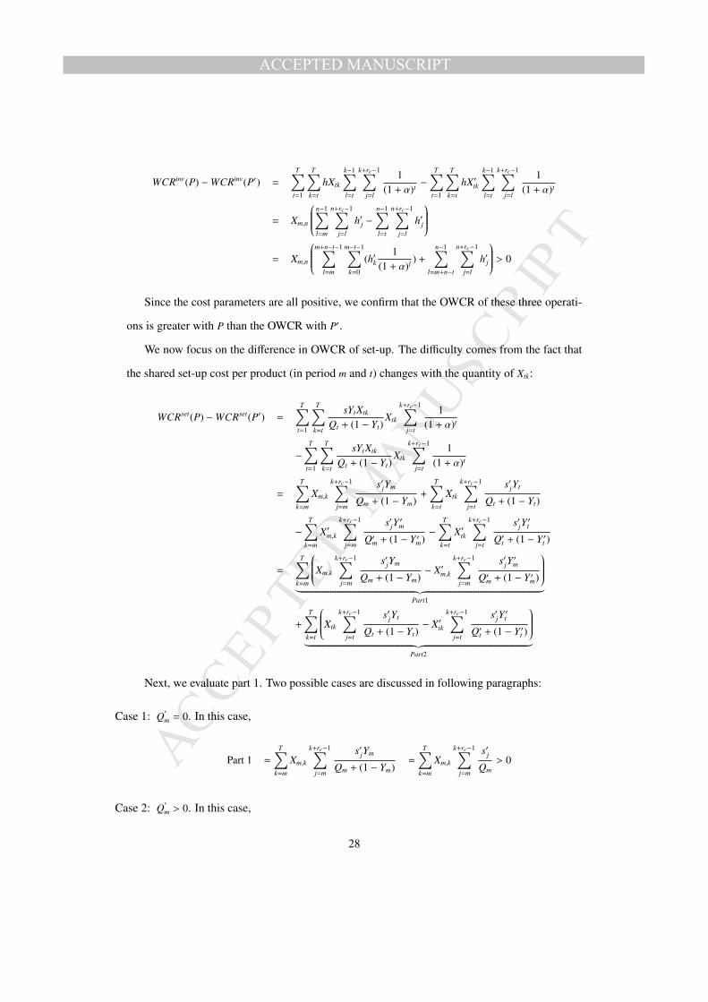
Since the cost parameters are all positive, we confirm that the OWCR of these three operati-
ons is greater with P than the OWCR with P′.
We now focus on the difference in OWCR of set-up. The difficulty comes from the fact that
the shared set-up cost per product (in period m and t) changes with the quantity of Xtk:
WCRset(P) −WCRset(P′) =
T∑t=1
T∑k=t
sYtXtk
Qt + (1 − Yt)Xtk
k+rc−1∑j=t
1(1 + α)t
−
T∑t=1
T∑k=t
sYtXtk
Qt + (1 − Yt)Xtk
k+rc−1∑j=t
1(1 + α)t
=
T∑k=m
Xm,k
k+rc−1∑j=m
s′jYm
Qm + (1 − Ym)+
T∑k=t
Xtk
k+rc−1∑j=t
s′jYt
Qt + (1 − Yt)
−
T∑k=m
X′m,k
k+rc−1∑j=m
s′jY′m
Q′m + (1 − Y ′m)−
T∑k=t
X′tk
k+rc−1∑j=t
s′jY′t
Q′t + (1 − Y ′t )
=
T∑k=m
Xm,k
k+rc−1∑j=m
s′jYm
Qm + (1 − Ym)− X′m,k
k+rc−1∑j=m
s′jY′m
Q′m + (1 − Y ′m)
︸ ︷︷ ︸Part1
+
T∑k=t
Xtk
k+rc−1∑j=t
s′jYt
Qt + (1 − Yt)− X′tk
k+rc−1∑j=t
s′jY′t
Q′t + (1 − Y ′t )
︸ ︷︷ ︸Part2
Next, we evaluate part 1. Two possible cases are discussed in following paragraphs:
Case 1: Q′
m = 0. In this case,
Part 1 =
T∑k=m
Xm,k
k+rc−1∑j=m
s′jYm
Qm + (1 − Ym)=
T∑k=m
Xm,k
k+rc−1∑j=m
s′jQm
> 0
Case 2: Q′
m > 0. In this case,
28

MANUSCRIP
T
ACCEPTED
ACCEPTED MANUSCRIPT
Part 1 =
T∑k=m
Xm,k
k+rc−1∑j=m
s′jYm
Qm + (1 − Ym)− X′m,k
k+rc−1∑j=m
s′jY′m
Q′m + (1 − Y ′m)
=
T∑k=m
Xm,k
k+rc−1∑j=m
s′jQm− X′m,k
k+rc−1∑j=m
s′jQ′m
=
1QmQ′m
T∑k=m
k+rc−1∑j=m
s′j(Xm,kQ
′
m − X′
m,kQm
)=
1QmQ′m
n+rc−1∑j=m
s′jXm,nQ′
m +
T∑k=m,k,n
k+rc−1∑j=m
s′j(X′
m,kQ′
m − X′
m,kQm
)=
1QmQ′m
n+rc−1∑j=m
s′jXm,nQ′
m +
T∑k=m,k,n
k+rc−1∑j=m
s′j(X′
m,kQ′
m − X′
m,k(Q′
m + Xm,n))
=1
QmQ′m
n+rc−1∑j=m
s′jXm,nQ′
m −
T∑k=m,k,n
k+rc−1∑j=m
s′jX′m,kXm,n
=
Xm,n
QmQ′m
n+rc−1∑j=m
s′jQ′
m −
T∑k=m,k,n
k+rc−1∑j=m
s′jX′m,k
=
Xm,n
QmQ′m
n+rc−1∑j=m
s′jt−1∑k=m
X′m,k −t−1∑k=m
k+rc−1∑j=m
s′jX′m,k
=
Xm,n
QmQ′m
t−1∑k=m
Xm,k(n+rc−1∑
j=m
s′j −k+rc−1∑
j=m
s′j)
=Xm,n
QmQ′m
t−1∑k=m
Xm,k
n+rc−1∑j=k+rc−1
s′j > 0
Thus, part 1 is positive in all cases. We then go through the part 2:
Part 2 =
T∑k=t
Xtk
k+rc−1∑j=t
s′jYt
Qt + (1 − Yt)− X′tk
k+rc−1∑j=t
s′jY′t
Q′t + (1 − Y ′t )
=
T∑k=t
Xtk
Qt
k+rc−1∑j=t
s′j −X′tkQ′t
k+rc−1∑j=t
s′j
=
1QtQ
′
t
T∑k=t
XtkQ′tk+rc−1∑
j=t
s′j − X′tkQt
k+rc−1∑j=t
s′j
=
1QtQ
′
t
T∑k=t
Xtk(Qt + Xm,n)k+rc−1∑
j=t
s′j − X′tkQt
k+rc−1∑j=t
s′j
=
1QtQ
′
t
T∑k=t
XtkXm,n
k+rc−1∑j=t
s′j − Qt(Xtk − X′tk)k+rc−1∑
j=t
s′j
29

MANUSCRIP
T
ACCEPTED
ACCEPTED MANUSCRIPT
=1
QtQ′
t
T∑k=t
XtkXm,n
k+rc−1∑j=t
s′j − QtXm,n
n+rc−1∑j=t
s′j
In order to determine the sign of part2, two following cases must be carefully examined:
Case A: Q′
t ≥ Qm. We haveXm,n
Q′t
n+rc−1∑j=n
s′j <Xm,n
Qm
n+rc−1∑j=n
s′j
Then, we attempt to compare this element with part 1:
Case A-1: Q′
m = 0. In this case,
Part 1 =
T∑k=m
Xm,k
Qm
k+rc−1∑j=m
s′j
=
T∑k=m,k,n
Xm,k
Qm
k+rc−1∑j=m
s′j +Xm,n
Qm
n+rc−1∑j=n
s′j
≥Xm,n
Qm
n+rc−1∑j=n
s′jq
≥Xm,n
Qm
n+rc−1∑j=n
s′j
Then, Part 1 + Part 2 ≥Xm,n
Qm
n+rc−1∑j=n
s′j −Xm,n
Q′t
n+rc−1∑j=n
s′j ≥ (Xm,n
Q′t−
Xm,n
Q′t)
n+rc−1∑j=n
s′j > 0 with Q′
t ≥ Qm
Case A-2: Q′
m > 0. In this case,
Part 1 =Xm,n
QmQ′m
t−1∑k=m
Xm,k
n+rc−1∑j=k+rc−1
s′j
=Xm,n
QmQ′m
t−1∑k=m
Xm,k(n+rc−1∑
j=m
s′j −k+rc−1∑
j=m
s′j)
≥Xm,n
QmQ′m
t−1∑k=m
Xm,k(n+rc−1∑
j=m
s′j −t+rc−1∑
j=m
s′j)
30

MANUSCRIP
T
ACCEPTED
ACCEPTED MANUSCRIPT
≥Xm,n
Qm(n+rc−1∑
j=m
s′j −t+rc−1∑
j=m
s′j)
≥Xm,n
Q′t(n+rc−1∑
j=m
s′j −t+rc−1∑
j=m
s′j)
=Xm,n
Q′t
n+rc−1∑j=t+rc−1
s′j (A.1)
Moreover, we have:
1QtQ
′
t
T∑k=t
XtkXm,n
k+rc−1∑j=t
s′j ≥
Xm,n
QtQ′
t
T∑k=t
Xtk
k+rc−1∑j=t
s′j ≥
Xm,n
QtQ′
t
T∑k=t
Xtk
t+rc−1∑j=t
s′j ≥
Xm,n
QtQ′
t
t+rc−1∑j=t
s′jT∑
k=t
Xtk ≥
Xm,n
Q′t
t+rc−1∑j=t
s′j (A.2)
Thus, with (A.1) and (A.2),
Part1 + Part2 ≥Xm,n
Q′t
n+rc−1∑j=t+rc−1
s′j +Xm,n
Q′t
t+rc−1∑j=t
s′j −Xm,n
Q′t
n+rc−1∑j=t
s′j ≥ 0
In this case, the sum of part 1 and part 2 is also positive.
Case B: Q′
t < Qm.
We distinguish again both cases of part 1:
Case B-1: Q′
m = 0. Impossible because Q′
t ≥ Qm.
Case B-2: Q′
m > 0. Part 1 can be transformed as follows:
31

MANUSCRIP
T
ACCEPTED
ACCEPTED MANUSCRIPT
Xm,n
QmQ′m
t−1∑k=m
Xm,k
n+rc−1∑j=k+rc−1
s′j ≥
Xm,n
QmQ′m
n+rc−1∑j=t+rc−2
s′jt−1∑k=m
Xm,k ≥
Xm,n
QmQ′m
n+rc−1∑j=t+rc−2
s′jQ′
m ≥
Xm,n
Qm
n+rc−1∑j=t+rc−2
s′j
Part 2 can be formulated as:
1QtQ
′
t
T∑k=t
XtkXm,n
k+rc−1∑j=t
s′j − QtXm,n
n+rc−1∑j=t
s′j
=
Xm,n
QtQ′
t
T∑k=t
Xtk
k+rc−1∑j=t
s′j − Qt
n+rc−1∑j=t
s′j
≥
Xm,n
QtQ′
t
t+rc−1∑j=t
s′j
T∑k=t
Xtk
− Qt
n+rc−1∑j=t
s′j
≥
Xm,n
QtQ′
t
t+rc−1∑j=t
s′jQt − Qt
n+rc−1∑j=t
s′j
≥
−Xm,n
Q′t
n+rc−1∑j=t+rc−1
s′j ≥
−Xm,n
Qm
n+rc−1∑j=t+rc−1
s′j
In consequence,
Part 1 + Part 2 =Xm,n
Qm
n+rc−1∑j=t+rc−2
s′j −Xm,n
Qm
n+rc−1∑j=t+rc−1
s′j ≥Xm,n
Qms′t+rc−2 ≥ 0
To summarize, the sum of part 1 and part 2 is positive in all cases which means P generates
a bigger OWCR financing cost than P′. To conclude, considering all above-mentioned compari-
sons, the NPV of revenue is equal with these two plans, but the NPV of the total cost is greater
with P. Therefore, we favor the P′ which has one less violation of ZIO property. In general, we
are able to deduce that the optimal planning is the ZIO type planning with no violations at all.
32