combined performance tests before installation of the
TRANSCRIPT
2008 JINST 3 P08003
PUBLISHED BY INSTITUTE OFPHYSICS PUBLISHING AND SISSA
RECEIVED: March 18, 2008REVISED: May 29, 2008ACCEPTED: July 7, 2008
PUBLISHED: August 8, 2008
Combined performance tests before installation ofthe ATLAS Semiconductor and Transition RadiationTracking Detectors
E. Abat, e,† A. Abdesselam, am T.N. Addy, s T.P.A. Åkesson, ab P.P. Allport, y
L. Andricek, ah F. Anghinolfi, i R. Apsimon, as E. Arik, e,† M. Arik, e N. Austin, y
O.K. Baker, bb E. Banas, l A. Bangert, ah G. Barbier, o S. Baron, i A.J. Barr, am
S. Basiladze, ag L.E. Batchelor, as R.L. Bates, q J.R. Batley, h M. Battistin, i G.A. Beck, aa
A. Beddall, e,1 A.J. Beddall, e,1 P.J. Bell, ac W.H. Bell, q A. Belymam, aa D.P. Benjamin, m
J. Bernabeu, ay H. Bertelsen, j S. Bethke, ah A. Bingul, e,1 A. Bitadze, i J.P. Bizzell, as
J. Blocki, l A. Bocci, m M. Bochenek, k J. Bohm, ap V.G. Bondarenko, a f P. Bonneau, i
C.N. Booth, au O. Brandt, am F.M. Brochu, h Z. Broklova, aq J. Broz, aq P.A. Bruckman deRenstrom, am,3 S. Burdin, y C.M. Buttar, q M. Capeáns Garrido, i L. Cardiel Sas, i
C. Carpentieri, n A.A. Carter, aa J.R. Carter, h A. Catinaccio, i S.A. Cetin, e,2 M. Chamizollatas, o D.G. Charlton, d A. Cheplakov, q S. Chouridou, at M.L. Chu, av V. Cindro, z
A. Ciocio, c J.V. Civera, ay A. Clark, o A.P. Colijn, ai T. Cornelissen, i M.J. Costa, ay
D. Costanzo, au J. Cox, am P. Cwetanski, t W. Dabrowski, k J. Dalmau, aa M. Dam, j
K.M. Danielsen, al H. Danielsson, i S. D’Auria, q I. Dawson, au P. de Jong, ai
M.D. Dehchar, am B. Demirkoz, i P. Dervan, y B. Di Girolamo, i S. Diez Cornell, ay
F. Dittus, i S.D. Dixon, au E. Dobson, am O.B. Dogan, e,† Z. Dolezal, aq B.A. Dolgoshein, a f
M. Donega, i M. D’Onofrio, o T. Donszelmann, au O. Dorholt, al J.D. Dowell, d Z. Drasal, aq
N. Dressnandt, an C. Driouchi, j R. Duxfield, au M. Dwuznik, k W.L. Ebenstein, m
S. Eckert, n P. Eerola, ab U. Egede,ab K. Egorov, t L.M. Eklund, i M. Elsing, i R. Ely,c
V. Eremin, ag C. Escobar, ay H. Evans, t P. Farthouat, i D. Fasching, ba O.L. Fedin, ao
L. Feld, n D. Ferguson, ba P. Ferrari, i D. Ferrere, o L. Fiorini, h J. Fopma, am A.J. Fowler, m
H. Fox,n R.S. French, au D. Froidevaux, i J.A. Frost, h J. Fuster, ay S. Gadomski, o,2
P. Gagnon, t B.J. Gallop, as F.C. Gannaway, aa C. Garcia, ay J.E. Garcia Navarro, ay
I.L. Gavrilenko, ae C. Gay,az N. Ghodbane, ah M.D. Gibson, as S.M. Gibson, am
K.G. Gnanvo, aa J. Godlewski, i T. Göttfert, ah S. Gonzalez, ba S. Gonzalez-Sevilla, ay
M.J. Goodrick, h A. Gorišek, z E. Gornicki, l M. Goulette, i Y. Grishkevich, ag
J. Grognuz, i J. Grosse-Knetter, f C. Haber,c R. Härtel, ah Z. Hajduk, l M. Hance,an
F.H. Hansen, j J.B. Hansen, j J.D. Hansen, j P.H. Hansen, j K. Hara,aw A. Harvey Jr., s
– 1 –

2008 JINST 3 P08003
M. Hauschild, i C. Hauviller, i B.M. Hawes, am R.J. Hawkings, i H.S. Hayward, y
S.J. Haywood, as F.E.W. Heinemann, am N.P. Hessey, ai J.C. Hill, h M.C. Hodgkinson, au
P. Hodgson, au T.I. Hollins, d A. Holmes, am R. Holt, as S. Hou,av D.F. Howell, am
W. Hulsbergen, i T. Huse,al Y. Ikegami, w Y. Ilyushenka, v C. Issever, am J.N. Jackson, y
V. Jain, t K. Jakobs, n R.C. Jared, ba G. Jarlskog, ab P. Jarron, i L.G. Johansen, b
P. Johansson, au M. Jones, am T.J. Jones, y D. Joos, n J. Joseph, ba P. Jovanovic, d
V.A. Kantserov, a f J. Kaplon, i M. Karagoz Unel, am F. Kayumov, ae P.T. Keener, an
G.D. Kekelidze, v N. Kerschen, au C. Ketterer, n S.H. Kim, aw D. Kisielewska, k
B. Kisielewski, l T. Kittelmann, j E.B. Klinkby, j P. Kluit, ai S. Kluth, ah B.R. Ko, m
P. Kodys, aq T. Koffas, i E. Koffeman, ai T. Kohriki, w T. Kondo, w N.V. Kondratieva, a f
S.P. Konovalov, ae S. Koperny, k H. Korsmo, ab S. Kovalenko, ao T.Z. Kowalski, k
K. Krüger, i V. Kramarenko, ag G. Kramberger, z M. Kruse, m P. Kubik, aq L.G. Kudin, ao
N. Kundu, am C. Lacasta, ay V.R. Lacuesta, ay W. Lau,am A-C. Le Bihan, i S.-C. Lee,av
R.P. Lefevre, o B.C. LeGeyt, an K.J.C. Leney, y C.G. Lester, h Z. Liang, av P. Lichard, i
W. Liebig, ai M. Limper, ai A. Lindahl, j S.W. Lindsay, y A. Lipniacka, b G. Llosa Llacer, ay
S. Lloyd, aa A. Loginov, bb C.W. Loh, az M. Lozano Fantoba, ay S. Lucas, i A. Lucotte, r
I. Ludwig, n J. Ludwig, n F. Luehring, t L. Luisa, ax J. Lynn, am M. Maaßen,n D. Macina, o
R. Mackeprang, j A. Macpherson, a C.A. Magrath, ai P. Majewski, au P. Malecki, l
V.P. Maleev,ao I. Mandi c,z M. Mandl, i M. Mangin-Brinet, o S. Marti i Garcia, ay
A.J. Martin, bb F.F. Martin, an T. Maruyama, aw R. Mashinistov, a f A. Mayne, au
K.W. McFarlane, s S.J. McMahon, as T.J. McMahon, d J. Meinhardt, n B.R. MelladoGarcia, ba C. Menot, i I. Messmer, n B. Mikulec, o M. Mikuž, z S. Mima,a j M. Minano, ay
B. Mindur, k V.A. Mitsou, ay P. Modesto, ay S. Moed,o B. Mohn, b R.M. Moles Valls, ay
J. Morin, aa M-C. Morone, o S.V. Morozov, a f J. Morris, aa H.G. Moser, ah
A. Moszczynski, l S.V. Mouraviev, ae A. Munar, an W.J. Murray, as K. Nagai, aa Y. Nagai,aw
D. Naito, a j K. Nakamura, aw I. Nakano, a j S.Y. Nesterov, ao F.M. Newcomer, an
R. Nicholson, au R.B. Nickerson, am T. Niinikoski, i N. Nikitin, ag R. Nisius, ah H. Ogren, t
S.H. Oh,m M. Olcese, p J. Olszowska, l M. Orphanides, au V. O’Shea,q W. Ostrowicz, l
B. Ottewell, am O. Oye,b E. Paganis, au M.J. Palmer, h M.A. Parker, h U. Parzefall, n
M.S. Passmore, i S. Pataraia, ah G. Pellegrini, ay H. Pernegger, i∗E. Perrin, o
V.D. Peshekhonov, v T.C. Petersen, i R. Petti, g A.W. Phillips, h P.W. Phillips, as
A. Placci, i K. Poltorak, k A. Poppleton, i M.J. Price, i K. Prokofiev, au O. Røhne,al
C. Rembser, i P. Reznicek, aq R.H. Richter, ah A. Robichaud-Veronneau, o
D. Robinson, h S. Roe, i O. Rohne, al A. Romaniouk, a f L.P. Rossi, p D. Rousseau, ak
G. Ruggiero, i K. Runge, n Y.F. Ryabov, ao A. Salzburger, u J. Sanchez, ay H. Sandaker, b
J. Santander, ay V.A. Schegelsky, ao D. Scheirich, aq J. Schieck, ah M.P. Schmidt, bb,†
C. Schmitt, i E. Sedykh, ao D.M. Seliverstov, ao A. Sfyrla, o T. Shin, s A. Shmeleva, ae
S. Sivoklokov, ag S.Yu. Smirnov, a f L. Smirnova, ag O. Smirnova, ab M. Söderberg, ab
A.O. Solberg, b V.V. Sosnovtsev, a f L. Sospedra Suay, ay H. Spieler, c G. Sprachmann, i
E. Stanecka, l S. Stapnes, al J. Stastny, ap M. Stodulski, l A. Stradling, ba B. Stugu, b
S. Subramania, t S.I. Suchkov, a f V.V. Sulin, ae R.R. Szczygiel, l R. Takashima, x
R. Tanaka,a j G. Tartarelli, ad P.K. Teng, av S. Terada,w V.O. Tikhomirov, ae P. Tipton, bb
– 2 –

2008 JINST 3 P08003
M. Titov, n K. Toms, ag A. Tonoyan, b D.R. Tovey, au A. Tricoli, as M. Turala, l M. Tyndel, as
F. Ukegawa, aw M. Ullan Comes, ay Y. Unno, w V. Vacek,ar S. Valkar, aq J.A. VallsFerrer, ay E. van der Kraaij, ai R. VanBerg, an V.I. Vassilakopoulos, s L. Vassilieva, ae
T. Vickey, ba G.H.A. Viehhauser, am E.G. Villani, as J.H. Vossebeld, y T. Vu Anh, o
R. Wall,bb R.S. Wallny, i C. Wang,m C.P. Ward,h R. Wastie, am M. Webel,n M. Weber,as
A.R. Weidberg, am P.M. Weilhammer, i C. Weiser, n P.S. Wells, i P. Werneke, ai
M.J. White, h D. Whittington, t A. Wildauer, i I. Wilhelm, aq H.H. Williams, an
J.A. Wilson, d M.W. Wolter, l S.L. Wu,ba A. Zhelezko, a f H.Z. Zhuau and A. Zsenei o
aCentre for Particle Physics, Department of Physics, University of Alberta,Edmonton, AB T6G 2G7, Canada
bUniversity of Bergen, Department for Physics and Technology,Allegaten 55, NO - 5007 Bergen, Norway
cLawrence Berkeley National Laboratory and University of California, Physics Division,MS50B-6227, 1 Cyclotron Road, Berkeley, CA 94720, United States of America
dSchool of Physics and Astronomy, University of Birmingham,Edgbaston, Birmingham B15 2TT, United Kingdom
eFaculty of Sciences, Department of Physics, Bogazici University,TR - 80815 Bebek-Istanbul, Turkey
f Physikalisches Institut der Universitaet Bonn, Nussallee12, D - 53115 Bonn, GermanygBrookhaven National Laboratory, Physics Department,Bldg. 510A, Upton, NY 11973, United States of America
hCavendish Laboratory, University of Cambridge,J J Thomson Avenue, Cambridge CB3 0HE, United Kingdom
iCERN, CH - 1211 Geneva 23, Switzerland, SwitzerlandjNiels Bohr Institute, University of Copenhagen,Blegdamsvej 17, DK - 2100 Kobenhavn 0, Denmark
kFaculty of Physics and Applied Computer Science of the AGH-University of Science andTechnology, (FPACS, AGH-UST), al. Mickiewicza 30, PL-30059 Cracow, Poland
l The Henryk Niewodniczanski Institute of Nuclear Physics, Polish Academy of Sciences,ul. Radzikowskiego 152, PL - 31342 Krakow, Poland
mDuke University, Department of Physics, Durham, NC 27708, United States of AmericanPhysikalisches Institut, Universitaet Freiburg,Hermann-Herder Str. 3, D - 79104 Freiburg i.Br., Germany
oUniversite de Geneve, Section de Physique,24 rue Ernest Ansermet, CH - 1211 Geneve 4, Switzerland
pINFN Genova and Università di Genova, Dipartimento di Fisica,via Dodecaneso 33, IT - 16146 Genova, Italy
qUniversity of Glasgow, Department of Physics and Astronomy,UK - Glasgow G12 8QQ, United Kingdom
rLaboratoire de Physique Subatomique et de Cosmologie, CNRS-IN2P3, Universite JosephFourier, INPG, 53 avenue des Martyrs, FR - 38026 Grenoble Cedex, France
sHampton University, Department of Physics, Hampton, VA 23668, United States of Americat Indiana University, Department of Physics, Swain Hall West,Room 117, 727 East Third St., Bloomington, IN 47405-7105, United States of America
uInstitut fuer Astro- und Teilchenphysik, Technikerstrasse 25, A - 6020 Innsbruck, Austria
– 3 –

2008 JINST 3 P08003
vJoint Institute for Nuclear Research, JINR Dubna, RU - 141 980 Moscow, RussiawKEK, High Energy Accelerator Research Organization, 1-1 Oho,Tsukuba-shi, Ibaraki-ken 305-0801, Japan
xKyoto University of Education, 1 Fukakusa, Fujimori,fushimi-ku, Kyoto-shi, JP - Kyoto 612-8522, Japan
yOliver Lodge Laboratory, University of Liverpool,P.O. Box 147, Oxford Street, UK - Liverpool L69 3BX, United Kingdom
zJožef Stefan Institute and Department of Physics, University of Ljubljana,SI-1001 Ljubljana, Slovenia
aaDepartment of Physics, Queen Mary, University of London,Mile End Road, UK - London E1 4NS, United Kingdom
abLunds Universitet, Fysiska Institutionen, Box 118, SE - 22100 Lund, SwedenacSchool of Physics and Astronomy, University of Manchester,
UK - Manchester M13 9PL, United KingdomadINFN Milano and Università di Milano, Dipartimento di Fisica,
via Celoria 16, IT - 20133 Milano, ItalyaeP.N. Lebedev Institute of Physics, Academy of Sciences,
Leninsky pr. 53, RU - 117 924 Moscow, Russiaa fMoscow Engineering & Physics Institute (MEPhI),
Kashirskoe Shosse 31, RU - 115409 Moscow, RussiaagLomonosov Moscow State University, Skobeltsyn Institute of Nuclear Physics,
RU - 119 992 Moscow Lenskie gory 1, RussiaahMax-Planck-Institut für Physik, (Werner-Heisenberg-Institut),
Föhringer Ring 6, 80805 München, GermanyaiNikhef National Institute for Subatomic Physics,
Kruislaan 409, P.O. Box 41882, NL - 1009 DB Amsterdam, Netherlandsa jOkayama University, Faculty of Science, Tsushimanaka 3-1-1, Okayama 700-8530, JapanakLAL, Univ. Paris-Sud, IN2P3/CNRS, Orsay, FrancealDepartment of Physics, University of Oslo, Blindern, NO - 0316 Oslo 3, Norway
amDepartment of Physics, Oxford University, Denys WilkinsonBuilding,Keble Road, Oxford OX1 3RH, United Kingdom
anUniversity of Pennsylvania, Department of Physics & Astronomy, 209 S. 33rd Street,Philadelphia, PA 19104, United States of America
aoPetersburg Nuclear Physics Institute, RU - 188 300 Gatchina, RussiaapInstitute of Physics, Academy of Sciences of the Czech Republic,
Na Slovance 2, CZ - 18221 Praha 8, Czech RepublicaqCharles University in Prague, Faculty of Mathematics and Physics, Institute of Particle and
Nuclear Physics, V Holesovickach 2, CZ - 18000 Praha 8, CzechRepublicarCzech Technical University in Prague, Zikova 4, CZ - 166 35 Praha 6, Czech RepublicasRutherford Appleton Laboratory, Science and Technology Facilities Council, Harwell Science
and Innovation Campus, Didcot OX11 0QX, United KingdomatUniversity of California Santa Cruz, Santa Cruz Institute for Particle Physics (SCIPP),
Santa Cruz, CA 95064, United States of AmericaauUniversity of Sheffield, Department of Physics & Astronomy,
Hounsfield Road, UK - Sheffield S3 7RH, United KingdomavInsitute of Physics, Academia Sinica, TW - Taipei 11529, TaiwanawUniversity of Tsukuba, Institute of Pure and Applied Sciences,
1-1-1 Tennoudai, Tsukuba-shi, JP - Ibaraki 305-8571, Japan
– 4 –
2008 JINST 3 P08003
axINFN Gruppo Collegato di Udine and Università di Udine, Dipartimento di Fisica,via delle Scienze 208, IT - 33100 Udine andINFN Gruppo Collegato di Udine and ICTP, Strada Costiera 11,IT - 34014 Trieste, Italy
ayInstituto de Física Corpuscular (IFIC), Centro Mixto UVEG-CSIC, Apdo. 22085, ES-46071Valencia; Dept. Física At., Mol. y Nuclear, Univ. of Valencia and Instituto de Microelectrónicade Barcelona (IMB-CNM-CSIC), 08193 Bellaterra, Barcelona, Spain
azUniversity of British Columbia, Dept of Physics,6224 Agricultural Road, CA - Vancouver, B.C. V6T 1Z1, Canada
baUniversity of Wisconsin, Department of Physics, Madison, WI 53706, United States of AmericabbYale University, Department of Physics,
PO Box 208121, New Haven CT, 06520-8121 , United States of America1Currently at Gaziantep University, Turkey2Currently at Dogus University, Istanbul3also at H. Niewodniczanski Institute of Nuclear Physics PAN, Cracow, Poland†DeceasedE-mail: [email protected]
ABSTRACT: The ATLAS (A Toroidal LHC ApparatuS) Inner Detector provides charged particletracking in the centre of the ATLAS experiment at the Large Hadron Collider (LHC). The InnerDetector consists of three subdetectors: the Pixel Detector, the Semiconductor Tracker (SCT), andthe Transition Radiation Tracker (TRT). This paper summarizes the tests that were carried out at thefinal stage of SCT+TRT integration prior to their installation in ATLAS. The combined operationand performance of the SCT and TRT barrel and endcap detectors was investigated through a seriesof noise tests, and by recording the tracks of cosmic rays. This was a crucial test of hardware andsoftware of the combined tracker detector systems. The results of noise and cross-talk tests onthe SCT and TRT in their final assembled configuration, using final readout and supply hardwareand software, are reported. The reconstruction and analysis of the recorded cosmic tracks allowedtesting of the offline analysis chain and verification of basic tracker performance parameters, suchas efficiency and spatial resolution, in combined operationbefore installation.
KEYWORDS: Particle tracking detectors; Solid state detectors; Transition radiation detectors;Large detector systems for particle and astroparticle physics.
∗Corresponding Author.
c© 2008 IOP Publishing Ltd and SISSA http://www.iop.org/EJ/jinst/

2008 JINST 3 P08003
Contents
1. Introduction 2
2. Experimental setup 52.1 Trigger 7
2.1.1 Barrel trigger setup 72.1.2 Endcap trigger setup 7
3. Detector readout and event reconstruction 83.1 Detector control system 8
3.1.1 SCT DCS 93.1.2 TRT DCS 11
3.2 Data acquisition 133.2.1 SCT DAQ 133.2.2 TRT DAQ 133.2.3 Trigger and synchronization 14
3.3 Simulation and reconstruction software 153.3.1 Detector description 153.3.2 Simulation 153.3.3 Reconstruction 173.3.4 Conditions database 20
3.4 Monitoring 213.4.1 Event filter monitoring 213.4.2 SCT specialized monitoring 233.4.3 TRT specialized monitoring 24
4. Tests with random triggers and calibration runs 264.1 SCT noise performance 26
4.1.1 Results from module calibration 264.1.2 Results from random triggers 27
4.2 TRT noise studies 33
5. Tests with cosmic triggers 365.1 Alignment and calibration 36
5.1.1 Alignment of the SCT and TRT 365.1.2 Alignment of the SCT 375.1.3 Comparison with the photogrammetry measurements 385.1.4 Relative alignment between the SCT and TRT 395.1.5 Alignment of the TRT 405.1.6 Alignment summary 425.1.7 TRT drift time calibration 42
– 1 –
2008 JINST 3 P08003
5.2 Tracking performance 465.3 SCT performance 49
5.3.1 Timing 505.3.2 Efficiency 505.3.3 SCT resolution 53
5.4 TRT performance 555.4.1 TRT efficiency 555.4.2 TRT resolution 56
6. Conclusions 57
1. Introduction
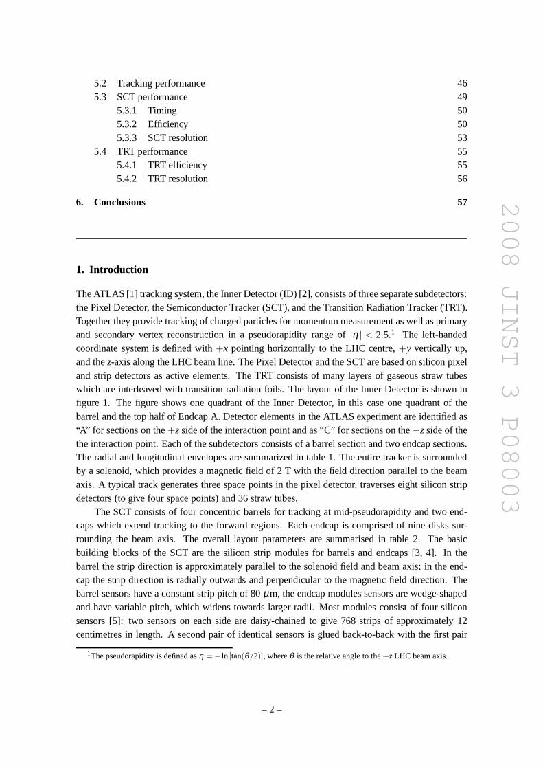
The ATLAS [1] tracking system, the Inner Detector (ID) [2], consists of three separate subdetectors:the Pixel Detector, the Semiconductor Tracker (SCT), and the Transition Radiation Tracker (TRT).Together they provide tracking of charged particles for momentum measurement as well as primaryand secondary vertex reconstruction in a pseudorapidity range of |η | < 2.5.1 The left-handedcoordinate system is defined with+x pointing horizontally to the LHC centre,+y vertically up,and thez-axis along the LHC beam line. The Pixel Detector and the SCT are based on silicon pixeland strip detectors as active elements. The TRT consists of many layers of gaseous straw tubeswhich are interleaved with transition radiation foils. Thelayout of the Inner Detector is shown infigure 1. The figure shows one quadrant of the Inner Detector, in this case one quadrant of thebarrel and the top half of Endcap A. Detector elements in the ATLAS experiment are identified as“A” for sections on the+zside of the interaction point and as “C” for sections on the−zside of thethe interaction point. Each of the subdetectors consists ofa barrel section and two endcap sections.The radial and longitudinal envelopes are summarized in table 1. The entire tracker is surroundedby a solenoid, which provides a magnetic field of 2 T with the field direction parallel to the beamaxis. A typical track generates three space points in the pixel detector, traverses eight silicon stripdetectors (to give four space points) and 36 straw tubes.
The SCT consists of four concentric barrels for tracking at mid-pseudorapidity and two end-caps which extend tracking to the forward regions. Each endcap is comprised of nine disks sur-rounding the beam axis. The overall layout parameters are summarised in table 2. The basicbuilding blocks of the SCT are the silicon strip modules for barrels and endcaps [3, 4]. In thebarrel the strip direction is approximately parallel to thesolenoid field and beam axis; in the end-cap the strip direction is radially outwards and perpendicular to the magnetic field direction. Thebarrel sensors have a constant strip pitch of 80µm, the endcap modules sensors are wedge-shapedand have variable pitch, which widens towards larger radii.Most modules consist of four siliconsensors [5]: two sensors on each side are daisy-chained to give 768 strips of approximately 12centimetres in length. A second pair of identical sensors isglued back-to-back with the first pair
1The pseudorapidity is defined asη = − ln [tan(θ/2)], whereθ is the relative angle to the+zLHC beam axis.
– 2 –
2008 JINST 3 P08003
Figure 1. Schematic drawing of one quadrant of the ATLAS Inner Detector.
Table 1. Radial and longitudinal envelopes of the Pixel, SCT and TRT detector sections.
Pixel 45.5< r < 242 mm|z| < 3092 mm
SCT Barrel 255< r < 549 mm|z| < 805 mm
SCT Endcap 251< r < 610 mm810< |z| < 2797 mm
TRT Barrel 554< r < 1082 mm|z| < 780 mm
TRT Endcap 617< r < 1106 mm827< |z| < 2744 mm
at a stereo angle of 40 mrad to provide space points. The innermodules of the endcap disks areshorter and consist of just two sensors with the same stereo angle. The module strips are read outby 12 radiation-hard ABCD3TA frontend readout chips [6]. The readout ASICs are integrated ona multi-layer Kapton-Cu flex circuit and are connected to thesilicon strips by wire bonds. Theflex circuit is mounted above the silicon sensors in the barrel modules and at the end of the siliconsensors in the endcap modules. The hit information is “binary”: only the channel address of a hitstrip is read out optically from each module side to the counting room; no analogue information ofthe signal is provided during normal running.
The TRT barrel contains up to 73 layers of straws interleavedwith polypropylene fibres andthe TRT endcap consists of 160 straw planes interleaved withpolypropylene foils, which providetransition radiation for electron identification. In the TRT barrel the straw direction is parallel tothe beam direction, in the endcap the straw direction is radially outwards. The barrel TRT [7] isdivided into three rings of 32 modules each, supported at each end by a space frame, which isthe main component of the barrel support structure. Each TRTendcap [8] consists of 20 wheelswith eight straw layers per wheel. In the endcap, the straw axis is radial and the anode wire is
– 3 –
2008 JINST 3 P08003
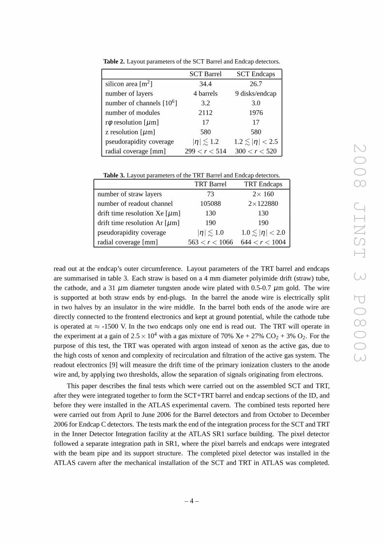
Table 2. Layout parameters of the SCT Barrel and Endcap detectors.
SCT Barrel SCT Endcaps
silicon area [m2] 34.4 26.7number of layers 4 barrels 9 disks/endcapnumber of channels [106] 3.2 3.0number of modules 2112 1976rφ resolution [µm] 17 17z resolution [µm] 580 580pseudorapidity coverage |η | . 1.2 1.2. |η | < 2.5radial coverage [mm] 299< r < 514 300< r < 520
Table 3. Layout parameters of the TRT Barrel and Endcap detectors.
TRT Barrel TRT Endcaps
number of straw layers 73 2× 160number of readout channel 105088 2×122880drift time resolution Xe [µm] 130 130drift time resolution Ar [µm] 190 190pseudorapidity coverage |η | . 1.0 1.0. |η | < 2.0radial coverage [mm] 563< r < 1066 644< r < 1004
read out at the endcap’s outer circumference. Layout parameters of the TRT barrel and endcapsare summarised in table 3. Each straw is based on a 4 mm diameter polyimide drift (straw) tube,the cathode, and a 31µm diameter tungsten anode wire plated with 0.5-0.7µm gold. The wireis supported at both straw ends by end-plugs. In the barrel the anode wire is electrically splitin two halves by an insulator in the wire middle. In the barrelboth ends of the anode wire aredirectly connected to the frontend electronics and kept at ground potential, while the cathode tubeis operated at≈ -1500 V. In the two endcaps only one end is read out. The TRT will operate inthe experiment at a gain of 2.5×10⁴ with a gas mixture of 70% Xe + 27% CO2 + 3% O2. For thepurpose of this test, the TRT was operated with argon insteadof xenon as the active gas, due tothe high costs of xenon and complexity of recirculation and filtration of the active gas system. Thereadout electronics [9] will measure the drift time of the primary ionization clusters to the anodewire and, by applying two thresholds, allow the separation of signals originating from electrons.
This paper describes the final tests which were carried out onthe assembled SCT and TRT,after they were integrated together to form the SCT+TRT barrel and endcap sections of the ID, andbefore they were installed in the ATLAS experimental cavern. The combined tests reported herewere carried out from April to June 2006 for the Barrel detectors and from October to December2006 for Endcap C detectors. The tests mark the end of the integration process for the SCT and TRTin the Inner Detector Integration facility at the ATLAS SR1 surface building. The pixel detectorfollowed a separate integration path in SR1, where the pixelbarrels and endcaps were integratedwith the beam pipe and its support structure. The completed pixel detector was installed in theATLAS cavern after the mechanical installation of the SCT and TRT in ATLAS was completed.
– 4 –

2008 JINST 3 P08003
Due to the integration and installation requirements for the ID, the pixel detector did not participatein the tests reported here.
The goals of the combined tests with the SCT and TRT were to test the noise performance ofthe combined detectors, to verify the absence of cross-talk, and to obtain experience in combineddetector operation in preparation for pit commissioning activities. The performance checks con-sisted of a series of noise tests with random triggers and calibration-mode noise tests, followed bydata taking to record cosmic ray tracks in the SCT and TRT. Thedetector sections used for thetests were limited by the size of the test system available onthe surface integration facility. In thetests approximately one quarter of both the SCT Barrel and Endcap C were powered and read outtogether with one-eighth of the TRT Barrel and one-sixteenth of the TRT Endcap C. Other sectionsof the detectors were not cooled, powered, or read out.
The full ATLAS offline software was used to analyze the cosmicray data. Key parts of thesoftware were tested during the combined operation. These software packages, such as the moni-toring, the reconstruction chain, and the calibration and alignment algorithms, will also be used fordata taken with colliding beams. The reconstruction and analysis of the recorded tracks allowed usto test the software chain and correct inconsistencies (e.g., in the detector description). The offlinesoftware was also used to check if the performance of the detector (efficiencies and resolutions) arewithin specifications.
2. Experimental setup
The tests described in this note were performed at the CERN Inner Detector Integration facilityat the ATLAS SR1 with the fully assembled SCT and TRT barrel and with one of the two SCTand TRT endcaps. Specifically, the endcap which is now installed on “Side C” of the ATLASexperiment was used.
Each SCT and TRT barrel or endcap was first assembled independently. For the SCT thisprocess was carried out at different assembly sites, while for the TRT the entire process was under-taken at SR1. The completed SCT barrel and endcaps were then inserted into the correspondingTRT subdetectors.
For the insertion of the SCT into the TRT, the SCT was supported on a cantilever frame asshown in the foreground of figure 2 (left) for the barrel. Meanwhile the completed TRT was trans-ferred into the final support and lifting frame, which was also used for the transport to the pit, andwhich can be seen in the background of figure 2 (left). The TRT was then guided on rails over theSCT (shown in figure 2 (right) for the endcap). During the movement the alignment and concen-tricity of the subdetectors were repeatedly verified, as wasthe electrical isolation of the SCT, TRTand support tooling. The clearance between the barrel portions of the SCT and the TRT is typically1 mm. After the insertion was completed, the SCT was positioned on rails inside the TRT with amechanical precision of≈250µm and a survey was carried out. The mechanical survey of the SCTand TRT barrel shows a horizontal displacement of∆x=0.3 mm and a rotation around they-axis of0.221 mrad of the SCT with respect to the TRT barrel.
For the final tests on the completed barrel, two opposite sectors of the SCT and TRT werecabled and tested. The connected sectors comprised 1/8 of the TRT and 468 modules, equivalent toapproximately one quarter, of the SCT barrel as shown on the right side of figure 3. For Endcap C
– 5 –

2008 JINST 3 P08003
Figure 2. Insertion of the SCT barrel into the TRT barrel (left) prior to their combined test in SR1. The rightphotograph shows the insertion of the SCT endcap into the TRTendcap before the SCT+TRT endcap weretested together.
Figure 3. Left: photo of the ID Barrel setup for the cosmic test; right:the configuration of module groupschosen for this test.
one quadrant of the SCT, consisting of 247 endcap modules, and 1/16 of the TRT Endcap WheelsA and B were connected to the supply and readout system. “Wheel A” denotes the twelve 8-planestraw wheels closest to the barrel (labelled 1 to 12 in figure 1) and “Wheel B” the eight 8-planestraw wheels farthest from the barrel (labelled 1 to 8 in figure 1). Care was taken to emulate thefinal setup in the pit, in particular for the service routing and detector grounding. Detectors andsupport structures were electrically isolated from each other. The detector grounds were connectedtogether in a star-point configuration similar to the one in the final configuration.
After the completion of the combined test of the SCT+TRT barrel detectors, they were installedas one package in the ATLAS cavern in August 2006. The SCT+TRTsections of endcap A wereinstalled in the ATLAS cavern in May 2007 and the SCT+TRT sections of endcap C in June 2007.
– 6 –

2008 JINST 3 P08003
2.1 Trigger
The following scintillator setups were implemented to record cosmic rays in the active barrel andendcap portions of the SCT and TRT.
2.1.1 Barrel trigger setup
For the barrel setup, cosmic rays were triggered using threelayers of Eljen EJ-200 scintillators2 ofdimension 144 cm× 40 cm× 2.5 cm, as shown in figure 4.
The three scintillators were arranged so that a wide angulardistribution of the cosmic raymuons would hit the scintillators as well as the instrumented sectors of the TRT and SCT. One ofthe scintillators was placed above the detector (HSC1), oneof them below (HSC2), and anotherunder the concrete floor (HSC3). The cosmic trigger was formed by looking for coincident hitsin the top and middle layers. The output of the third scintillator was also recorded to allow for anoptional offline energy cutoff of around 170 MeV (corresponding to a 15 cm thickness of concrete)by requiring an additional coincidence with the third scintillator.
The time of an output pulse emerging from one of the two Hamamatsu R2150 phototubes at-tached to both ends of the scintillators may differ from the other by a few nanoseconds dependingon where the particle intersects the scintillator. Therefore, a LeCroy Model 624 Octal Meantimerwas used to equalize the photon transit time by providing an output pulse at a fixed time, inde-pendent of where the impact occurred. In this way a 0.5 ns timeresolution was achieved in thetime-of-flight measurement. The scintillator coincidencerate, which was used to trigger the detec-tor readout, was 2.4 Hz. A total of 450000 events were recorded for the barrel test.
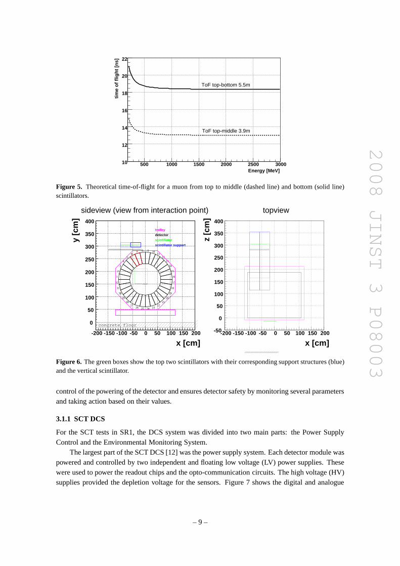
Figure 5 shows that the time-of-flight is independent of the energy of the cosmic muon forenergies above 600 MeV. The time-of-flight from the top scintillator (HSC1) to the bottom scintil-lator (HSC3) was used to cut away noise events (i.e., fake triggers) which can be recognized by anunphysical value for the computed time-of-flight. Other than in the rejection of noise triggers, thescintillator data were not used to select specific event samples. No momentum selection, based onscintillator data, was carried out during the offline analysis.
In addition, the charge deposited can be measured. This is important for ensuring that theevent has been triggered by a charged particle. The charge resolution is on the order of 100 fC.
2.1.2 Endcap trigger setup
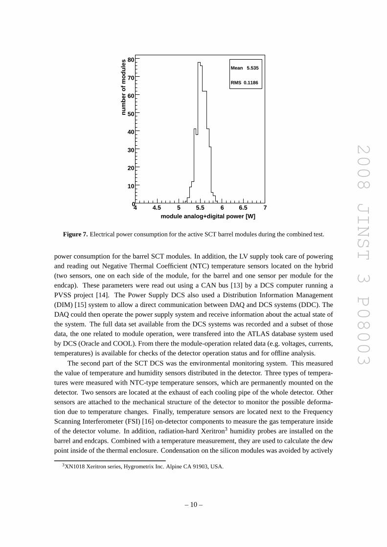
For the endcap setup, two of the three scintillators from thebarrel setup were reused and placedon top of the endcap while a third scintillator of size 50 cm× 60 cm was placed vertically in frontof the endcap as shown in figure 6. This layout balances the competing demands of selecting longtracks in the endcaps and having an acceptable rate of tracks. Information about the time-of-flightwas not available in this setup. The trigger rate for coincidence of the endcap trigger scintillatorswas 0.7 Hz. Due to the low scintillator trigger rate additional data samples were recorded usingTRT endcap frontend signals to enhance the track sample in the SCT for SCT studies at a triggerrate of 25 Hz. The scintillator trigger resulted in a rate of reconstructed tracks of 0.17 tracks/s, theTRT frontend trigger in a rate of 1.38 tracks/s. A total of 2.5million events were recorded for theendcap test.
2Eljen Technology, PO Box 870, 300 Crane Street, Sweetwater TX 79556, USA
– 7 –

2008 JINST 3 P08003
[cm]-200 -150 -100 -50 0 50 100 150 200
[cm
]
-200
-100
0
100
200
300
400
1
2
3
4
5
67
8 9 10 1112
13
14
15
16
17
18
19
20
21
2223
2425262728
29
30
31
32
78
2324
1
concrete floor
HSC1
HSC2
HSC3
Inner Detector
Figure 4. The boxes marked as “HSC1”, “HSC2”, “HSC3”, one above the Inner Detector and two below,represent the scintillators used for trigging on cosmic rays in the barrel region. Each scintillator was readout with two photomultipliers, one at each end. The hatched box just below HSC2 represents the concretefloor.
3. Detector readout and event reconstruction
3.1 Detector control system
The Detector Control System (DCS) serves two purposes during detector operation. It allows
– 8 –
2008 JINST 3 P08003
Energy [MeV]500 1000 1500 2000 2500 3000
time
of fl
ight
[ns]
10
12
14
16
18
20
22
ToF top-bottom 5.5m
ToF top-middle 3.9m
Figure 5. Theoretical time-of-flight for a muon from top to middle (dashed line) and bottom (solid line)scintillators.
x [cm]-200 -150 -100 -50 100 150 200
y [c
m]
0
50
100
150
200
250
300
350
400
1
2
3
4
56
7 8 9 1011
12
13
14
15
16
17
18
19
20
2122
2324252627
28
29
30
31
32
76
trolley
detectorscintillator
scintillator support
sideview (view from interaction point)
x [cm]-200 -150 -100 -50 100 150 200
z [c
m]
-50
0
50
100
150
200
250
300
350
400
topview
concrete floor
0 50 0 50
Figure 6. The green boxes show the top two scintillators with their corresponding support structures (blue)and the vertical scintillator.
control of the powering of the detector and ensures detectorsafety by monitoring several parametersand taking action based on their values.
3.1.1 SCT DCS
For the SCT tests in SR1, the DCS system was divided into two main parts: the Power SupplyControl and the Environmental Monitoring System.
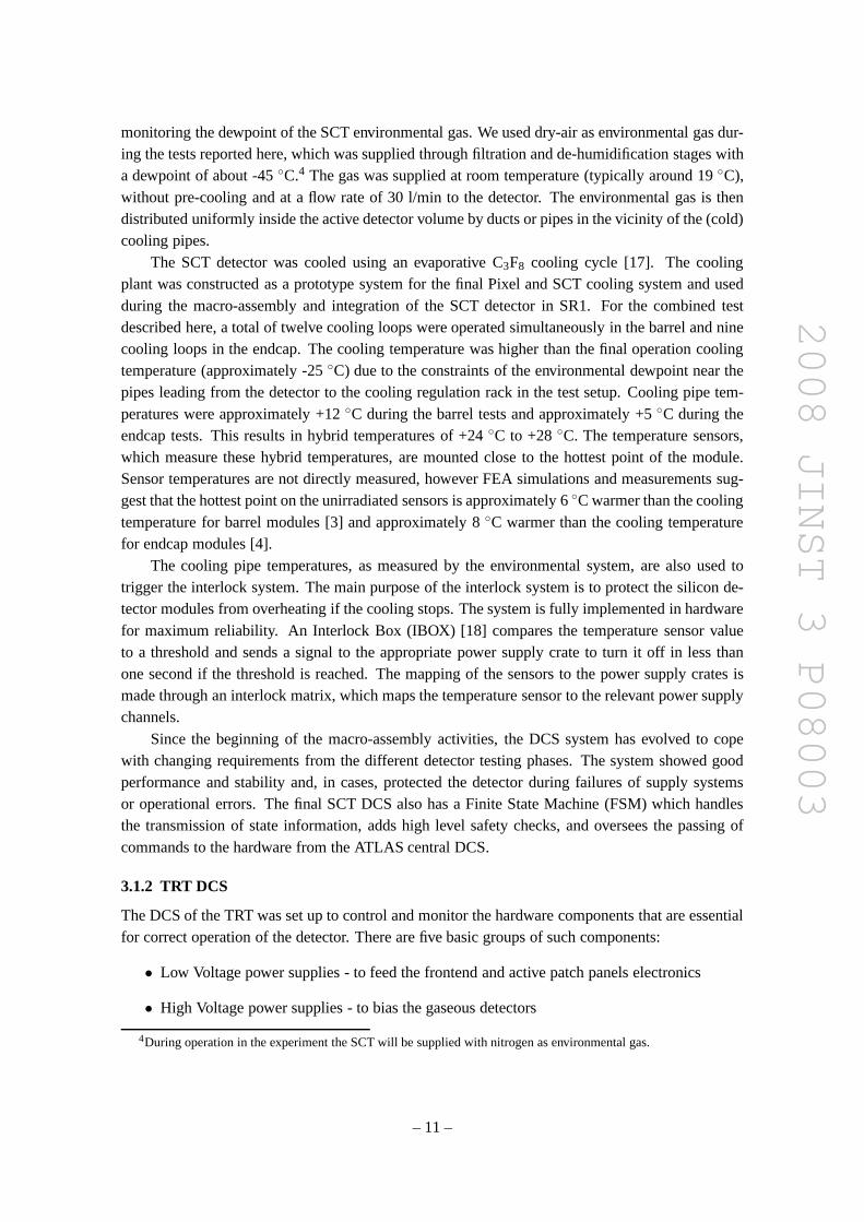
The largest part of the SCT DCS [12] was the power supply system. Each detector module waspowered and controlled by two independent and floating low voltage (LV) power supplies. Thesewere used to power the readout chips and the opto-communication circuits. The high voltage (HV)supplies provided the depletion voltage for the sensors. Figure 7 shows the digital and analogue
– 9 –
2008 JINST 3 P08003
Mean 5.535
RMS 0.1186
module analog+digital power [W]4 4.5 5 5.5 6 6.5 7
num
ber
of m
odul
es
0
10
20
30
40
50
60
70
80Mean 5.535
RMS 0.1186
Figure 7. Electrical power consumption for the active SCT barrel modules during the combined test.
power consumption for the barrel SCT modules. In addition, the LV supply took care of poweringand reading out Negative Thermal Coefficient (NTC) temperature sensors located on the hybrid(two sensors, one on each side of the module, for the barrel and one sensor per module for theendcap). These parameters were read out using a CAN bus [13] by a DCS computer running aPVSS project [14]. The Power Supply DCS also used a Distribution Information Management(DIM) [15] system to allow a direct communication between DAQ and DCS systems (DDC). TheDAQ could then operate the power supply system and receive information about the actual state ofthe system. The full data set available from the DCS systems was recorded and a subset of thosedata, the one related to module operation, were transfered into the ATLAS database system usedby DCS (Oracle and COOL). From there the module-operation related data (e.g. voltages, currents,temperatures) is available for checks of the detector operation status and for offline analysis.
The second part of the SCT DCS was the environmental monitoring system. This measuredthe value of temperature and humidity sensors distributed in the detector. Three types of tempera-tures were measured with NTC-type temperature sensors, which are permanently mounted on thedetector. Two sensors are located at the exhaust of each cooling pipe of the whole detector. Othersensors are attached to the mechanical structure of the detector to monitor the possible deforma-tion due to temperature changes. Finally, temperature sensors are located next to the FrequencyScanning Interferometer (FSI) [16] on-detector components to measure the gas temperature insideof the detector volume. In addition, radiation-hard Xeritron3 humidity probes are installed on thebarrel and endcaps. Combined with a temperature measurement, they are used to calculate the dewpoint inside of the thermal enclosure. Condensation on the silicon modules was avoided by actively
3XN1018 Xeritron series, Hygrometrix Inc. Alpine CA 91903, USA.
– 10 –
2008 JINST 3 P08003
monitoring the dewpoint of the SCT environmental gas. We used dry-air as environmental gas dur-ing the tests reported here, which was supplied through filtration and de-humidification stages witha dewpoint of about -45◦C.4 The gas was supplied at room temperature (typically around 19 ◦C),without pre-cooling and at a flow rate of 30 l/min to the detector. The environmental gas is thendistributed uniformly inside the active detector volume byducts or pipes in the vicinity of the (cold)cooling pipes.
The SCT detector was cooled using an evaporative C3F8 cooling cycle [17]. The coolingplant was constructed as a prototype system for the final Pixel and SCT cooling system and usedduring the macro-assembly and integration of the SCT detector in SR1. For the combined testdescribed here, a total of twelve cooling loops were operated simultaneously in the barrel and ninecooling loops in the endcap. The cooling temperature was higher than the final operation coolingtemperature (approximately -25◦C) due to the constraints of the environmental dewpoint nearthepipes leading from the detector to the cooling regulation rack in the test setup. Cooling pipe tem-peratures were approximately +12◦C during the barrel tests and approximately +5◦C during theendcap tests. This results in hybrid temperatures of +24◦C to +28◦C. The temperature sensors,which measure these hybrid temperatures, are mounted closeto the hottest point of the module.Sensor temperatures are not directly measured, however FEAsimulations and measurements sug-gest that the hottest point on the unirradiated sensors is approximately 6◦C warmer than the coolingtemperature for barrel modules [3] and approximately 8◦C warmer than the cooling temperaturefor endcap modules [4].
The cooling pipe temperatures, as measured by the environmental system, are also used totrigger the interlock system. The main purpose of the interlock system is to protect the silicon de-tector modules from overheating if the cooling stops. The system is fully implemented in hardwarefor maximum reliability. An Interlock Box (IBOX) [18] compares the temperature sensor valueto a threshold and sends a signal to the appropriate power supply crate to turn it off in less thanone second if the threshold is reached. The mapping of the sensors to the power supply crates ismade through an interlock matrix, which maps the temperature sensor to the relevant power supplychannels.
Since the beginning of the macro-assembly activities, the DCS system has evolved to copewith changing requirements from the different detector testing phases. The system showed goodperformance and stability and, in cases, protected the detector during failures of supply systemsor operational errors. The final SCT DCS also has a Finite State Machine (FSM) which handlesthe transmission of state information, adds high level safety checks, and oversees the passing ofcommands to the hardware from the ATLAS central DCS.
3.1.2 TRT DCS
The DCS of the TRT was set up to control and monitor the hardware components that are essentialfor correct operation of the detector. There are five basic groups of such components:
• Low Voltage power supplies - to feed the frontend and active patch panels electronics
• High Voltage power supplies - to bias the gaseous detectors
4During operation in the experiment the SCT will be supplied with nitrogen as environmental gas.
– 11 –

2008 JINST 3 P08003
• Temperature sensor - for checks of the FE electronics operation temperature
• Cooling system - C6F14 cooling of the FE electronics
• Active gas system
Only the temperature sensors mounted on the detector parts (cooling plates, electronics boards,modules shells) were of the final type. All other systems consisted of the hardware available atthe time. While the interfaces to the hardware were specifically built for the SR1 setup, the higherlayers of control software were prototypes of the final ATLASsystem, hence the setup was used toqualify the different procedures and actions of the final system. The TRT was operated during thetests in SR1 with an active gas mix of Ar:CO2 in the ratio of 70%:30%.
Three PL500 power crates manufactured by Wiener Plein & BausElectronics5 were used toprovide low voltage to the TRT. They contained eight channels each allowing us to create an LVpartitioning similar to the final architecture planned for the experiment. The control of the crateswas done using the CAN bus as the physical layer and using the OPC server as a higher-levelcontrol. The output of the power supplies (analogue positive/negative and digital voltages) fedthe LV patch panels (LVPP), which in turn distributed voltage lines to the individual electronicboards on the detector. The LVPP boards are controlled remotely via another CANbus branchand the CANOpen OPC protocol. The LVPP boards contain a standard ATLAS control module,ELMB [20], which serves as the measuring instrument for currents and voltages in individual lineswith its analogue segment, and as the communication driver,allowing the setting of the DACs forvoltage adjustment and a way to switch the regulators on or off via digital ports.
A CAEN 1527 system along with four 1833 boards6 was used to provide high voltage to theTRT straws. The software was built with the use of the CERN JCOP FrameWork toolkits [19].The setup allowed for the control and monitoring of voltagesand currents and was also capableof performing predefined actions on HV channels or modules consisting of several consecutiveoperations. For operation in SR1 we used a typical HV of -1500V applied to the straw tubes.
The TRT detector is equipped with several temperature sensors that monitored sensitive pointsof the apparatus. The temperatures of frontend electronicsboards are monitored by NTC sensors,while cooling elements and detector mechanics are monitored with PT1000 probes. The signals arefed to the ELMB module, which is read out via the CANbus and CANOpen OPC server. Limits areset on the temperature values, with the system configured to give a warning after crossing the firstthreshold and to switch the low voltage power supplies off when a dangerous temperature limit isreached.
For the TRT setup in SR1 the cooling unit was controlled via the local programmable logiccontroller (PLC) and the control DCS software had only monitoring functions. However the sta-tus of the unit was coupled to the low voltage system through ahardware-based interlock system,allowing the powering down of the detector in the case of a cooling failure. For the barrel a tem-porary interlock system using several NTC temperature sensors, which monitored on-barrel elec-tronic temperatures, was connected to special comparator logic which switches the power suppliesoff when the temperature threshold is exceeded.
5W-IE-NE-R, Plein & Baus GmbH, Müllersbaum 20, D - 51399 Burscheid, Germany6CAEN S.p.A., Via Vetraia, 11, I-55049 Viareggio (LU), Italy
– 12 –

2008 JINST 3 P08003
3.2 Data acquisition
3.2.1 SCT DAQ
Control, readout, and online calibration of the SCT were performed using the SctRodDaq [21],which was developed within the ATLAS TDAQ software framework [23]. Multiple c++ and Javaapplications can communicate across multiple processors using CORBA.7 The hardware part ofthe SctRodDaq system in SR1 was comprised of several PCs, a 6UVME crate for Trigger TimingControl (TTC) specific modules, and a 9U VME64x crate housing12 Readout Driver Modules(RODs) [25], 12 Back of Crate cards (BOCs), and a Timing Interface Module (TIM). The RODsare used for the main control and data handling, whereas the BOCs provide the ROD interface tothe frontend modules and to the rest of the ATLAS DAQ chain. The TIM provides the interface tothe ATLAS TTC system. Each ROD/BOC pair is connected optically to up to 48 SCT modules,and to a single Readout Supervisor (ROS) PC.
The SCT uses a binary readout architecture based on the ABCD3TA chip [6] whereby a hit isregistered if a pulse height from the silicon microstrip detector channel exceeds a preset threshold.SctRodDaq operates in two modes. For calibration of the SCT modules, triggers are generatedinternally by the RODs or by the TIM and sent to the modules. Known test charges are injected bythe frontend chips and the occupancy (the fraction of triggered events for which the pulse heightexceeds the threshold) is determined as a function of threshold. The resulting threshold scan dataare extracted from the RODs via VME readout and analysed online to generate an optimised cali-bration, which is then applied for cosmics or physics data taking. For running in physics or cosmicsmode, the triggers (originating from collisions or cosmics) are sent to the frontend chips via theTTC system. Hit information arising from noise or cosmics are channeled event-by-event to theROS for subsequent event building. The data are then analysed offline or online for track recon-struction and tracking efficiency. For the tests presented here, we recorded for each hit the infor-mation in the triggered bunch-crossing cycle plus the hit information of the bunch-crossing cycleprior to and immediately after the trigger bunch crossing cycle. This “hit pattern” is then presentedin its binary form as e.g., “011” for a signal recorded in the trigger time bin (second bit), none inits preceding clock cycle, and a signal above threshold in the cycle after the triggered time bin.
3.2.2 TRT DAQ
The TRT data acquisition system was composed of two softwaretools: XTRT [24] for calibra-tion and parameter tuning, and the TRT DAQ for the collectionand storage of data generated byan external trigger source. Each tool was responsible for coordinating the actions of the frontendelectronics, which are mounted at the end of the straw chambers, and the “backend” electronics,prototypes of two different 9U VME modules located off-detector. A series of patch panels medi-ated the communcation between the frontend and the backend.They provided signal compensationand replication for signals going to the frontend, and further compensation for signals returning tothe backend.
The TRT makes use of two custom ASICs on the frontend electronics to detect both minimumionizing particles (low threshold) as well as transition radiation (high threshold). The analogue
7Common Object Request Broker Architecture define by the Object Management Group enables software compo-nents written in multiple computer languages and running onmultiple computers to work together.
– 13 –

2008 JINST 3 P08003
ASDBLR chip [26] provides a ternary output corresponding tothree states: below threshold, lowthreshold crossed, low and high threshold crossed. The analogue output currents are sent to acompanion DTMROC chip [27], which digitizes the analogue data and, upon receipt of a trigger,returns the data for 16 straws to a ROD backend module.
The XTRT program was used extensively for testing of prototype and production frontendelectronics. The tests included scans of timing and threshold parameters, the injection of testpulses to test the response of the frontend to known signal shapes and amplitudes, and the use of an“accumulate mode” in the digitizing chips to test the integration of the electronics with the gas andhigh voltage systems. The results of all tests, as well as a record of the hardware used in each test,were stored in a MySQL database, which provided read-only access to a web interface for easybrowsing of the results.
While XTRT was designed to track the response of the hardwareas various parameters werescanned, the TRT DAQ was designed to take data at a fixed point in parameter space. The TRTDAQ is a collection of c++ libraries and database objects, which are used to initialize and runan instance of the ATLAS TDAQ software framework [23]. The TRT DAQ is configured via adatabase, which contains instructions for all of the necessary ATLAS DAQ infrastructure as wellas specific parameters used for running the TRT back- and frontend electronics. The TRT specificparameters were extracted from the database which held the results of the XTRT scans.
Because the TRT DAQ was an instance of the ATLAS TDAQ framework, it scaled easily tocope with the amount of readout hardware available. For the barrel and endcap tests, the systemwas composed of two 9U VME crates for TRT backend hardware, one 6U VME crate for ATLASTTC hardware, a PC dedicated for event building and storage,and a PC used to control the TDAQinfrastructure.
3.2.3 Trigger and synchronization
The trigger system used for both noise tests and cosmic ray tests was based on the ATLAS TTCsystem hardware. This hardware facilitates the distribution of clock, reset, and trigger signals toone or more subsystems via fibreoptic links between a TTC Crate and a Readout Driver Crate. EachTTC “partition” contains hardware sufficient to trigger some subset of a single subsystem. Differentpartitions can be daisy-chained together by connecting themaster components of each partition,called the Local Trigger Processors. In the SR1 system tests, there were separate partitions for theTRT and for the SCT. In this case, one partition acted as the master, and the other as the slave. Thedistinction between master and slave was made in software, so the same cable connections couldbe used in either configuration.
To test systematic noise effects introduced by either subsystem on the other, two different noisetriggers were used. The first was a trigger at a fixed frequency(variable from a fraction of a Hz toseveral MHz), while the second was a pseudo-random pulser, the average frequency of which wastunable between several Hz and several kHz. Neither triggerwas synchronous with the 40 MHzclock used by the subsystems, so a synchronization of the trigger signal was performed in the TTCcrate. For noise data, the phase of the trigger with respect to the clock was not monitored.
For tests with cosmic rays, the trigger was generated in one of two different ways. For thebarrel tests, the scintillators described in section 2 provided a coincidence trigger designed to illu-minate the active readout regions. For the endcap, in addition to the scintillator trigger, the TRT
– 14 –
2008 JINST 3 P08003
self-trigger functionality was exploited. In this mode, the digital chips on the TRT frontend pro-vided a trigger if any of their associated straw channels went over threshold. These triggers werecollected by the TRT-TTC module, and used to create a multiplicity based trigger for the two sub-systems. The efficiency and fake rates were almost entirely determined by the selection of frontendthresholds, so that it was possible to obtain a reasonably pure and efficient trigger.
In the case of cosmic ray triggers, unlike the case of noise triggers, the phase of the asyn-chronous trigger signal with respect to the clock plays a crucial role. The trigger must be syn-chronized with the 40 MHz clock before it reaches the frontend electronics, so a measurementof this phase must be made before the data are collected. To determine this phase, two methodswere employed. In the first, the TRT-TTC module was given a trigger delay measurement (TDM)module, which received an asynchronous trigger signal and stored the resulting measurement inthe TRT event fragment written to disk. In the second method,a TDC was used to measure thephase of the scintillator trigger, the results of which werestored in an independent event fragment.Both methods were limited to scintillator triggers; no phase measurement was possible for the TRTself-trigger.
3.3 Simulation and reconstruction software
The offline software infrastructure developed in ATLAS to simulate and reconstruct the LHC datawas used for the first data taken by the Inner Detector in SR1. Thanks to the very flexible underlyingATHENA [28] framework, the necessary adaptations in the algorithms could be easily integrated.These adaptations were required in order to take into account the fact that particles are not producedin the middle of the detector and that they are not synchronized with the readout clock, but randomlygenerated.
3.3.1 Detector description
The detector description is a common service that provides the geometry (including alignmentcorrections) and material information. It is used in the simulation to create the Geant4 [29, 30]geometry and to emulate the response of the electronics. In addition, it is used by the differentsteps of the reconstruction. A specific detector description was created for the SR1 setup with nomagnetic field.
For track fitting purposes, a simplified version of the geometry was created from the sameservice. This tracking geometry, which is the result of simplifying the material description intolayers and volumes, allows for fast navigation. However, nodirect measurement of the momentumcan be done from the SR1 reconstructed tracks due to the lack of a magnetic field and thereforematerial effects cannot be taken into account during tracking, leading to an underestimation of theuncertainty of the measured track quantities.
3.3.2 Simulation
A simulation of cosmic ray events for the detectors as set up in SR1 was provided in order tofirst test the full reconstruction chain before data taking started and later to compare the data withsimulated events.
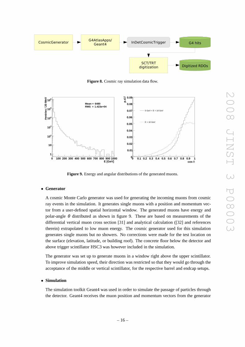
The data flow of the simulation (figure 8) contained the following steps:
– 15 –
2008 JINST 3 P08003
Figure 8. Cosmic ray simulation data flow.
E [GeV]0 100 200 300 400 500 600 700 800 900 1000
#ent
ries
/ 20
MeV
1
10
210
310
410
510
610Mean = 6480RMS = 1.423e+04
θcos 0 0.1 0.2 0.3 0.4 0.5 0.6 0.7 0.8 0.9 10
0.01
0.02
0.03
0.04
0.05
0.06
0.07
0.08
0.09
0 GeV < E < 10 GeV
E > 10 GeVp.
d.f
Figure 9. Energy and angular distributions of the generated muons.
• Generator
A cosmic Monte Carlo generator was used for generating the incoming muons from cosmicray events in the simulation. It generates single muons witha position and momentum vec-tor from a user-defined spatial horizontal window. The generated muons have energy andpolar-angleθ distributed as shown in figure 9. These are based on measurements of thedifferential vertical muon cross section [31] and analytical calculation ([32] and referencestherein) extrapolated to low muon energy. The cosmic generator used for this simulationgenerates single muons but no showers. No corrections were made for the test location onthe surface (elevation, latitude, or building roof). The concrete floor below the detector andabove trigger scintillator HSC3 was however included in thesimulation.
The generator was set up to generate muons in a window right above the upper scintillator.To improve simulation speed, their direction was restricted so that they would go through theacceptance of the middle or vertical scintillator, for the respective barrel and endcap setups.
• Simulation
The simulation toolkit Geant4 was used in order to simulate the passage of particles throughthe detector. Geant4 receives the muon position and momentum vectors from the generator
– 16 –

2008 JINST 3 P08003
and propagates the particle through a very detailed three-dimensional model of the detector,simulating the energy depositions throughout the detector.
• Trigger
A trigger algorithm was used to select those events which generated hits in both upper andmiddle scintillators (Barrel setup) or vertical scintillator (Endcap setup), respectively, andonly those were written to disk.
• Digitization
The digitization converts the simulated deposited energy to the Raw Data Objects (RDOs),which form the input objects to the reconstruction. It simulates effects such as the finite read-out resolution of the detectors and the electronic response. During this process the detectorelements which were not read out were masked.
The SCT digitization algorithm is described in ref. [33]. The algorithm loops over the de-posited energy in the detector elements and determines if the collected charge would pass thecomparator threshold of 1 fC. During the digitization a uniform noise level of 1500 electronsENC is added to the simulated signal data of all individual channels. It is also time-aware,in the sense that it integrates charge collection over one bunch crossing. Charges depositedafter this are not taken into account for the hit decision procedure.
The SCT digitization is interfaced to the conditions database for determining which modules,chips, and channels should be enabled for a given run number.Measured detector character-istics like channel specific noise and gain as well as configuration parameters such as appliedbias voltages and thresholds are also available from the conditions database, but those werenot used in this test.
Concerning the TRT, the digitization process simulates thedrift of charges from ionizationof the gas to the central wire, and records the drift time and time over threshold. It alsoadds the additional time introduced by the propagation fromthe impact point on the strawto the readout at the end of the straw. In addition, it simulates noise modeled from ATLASCombined Test Beam (CTB) data [34]. To account for the use of argon instead of xenon inthe combined tests, drift times were reduced by a factor of two-thirds and the detection ofhigh-signal hits was disabled.
The default ATLAS TRT digitization assumes that the particles originate from the interactionpoint, and for each straw there is a time offsetT0 taking this into account. However, in cosmicray events, the particles enter the top of TRT and leave through the bottom, so a differenttiming scheme was applied.
3.3.3 Reconstruction
A diagram representing the data flow of the reconstruction chain is shown in figure 10. It is de-signed to work with both simulated and real data provided that for the real case the data given outby the detectors are decoded and the corresponding RDOs created. The different steps of the chainare described below in more detail. The inner detector and tracking Event Data Model classes aredescribed in more detail in [35] and [36].
– 17 –

2008 JINST 3 P08003
Figure 10. Cosmic ray reconstruction data flow.
• Byte Stream convertersThe byte stream converters are responsible for decoding thedifferent ROD event fragmentsand creating a raw data object (RDO) for each recorded signal. The result is an SCT RDOper consecutive group of strips or an individual strip that had a signal (depending on whetherthe ROD is configured to run in “condensed” or “expanded” mode), and a TRT RDO per hitstraw. All the information written by the different detectors describing the signal is stored inthe RDO objects.
The converters use the ATHENA cabling service to map the ROD channel numbers to thecorresponding detector elements.
Since the cosmic trigger was not synchronized with the 40 MHzreadout clock the timedifference between the trigger and the next clock edge is also stored in the TRT RDO in thecase of the barrel setup to allow for a drift time correction.
Specific converters and RDO classes were developed in the same framework in order to storethe ADC and TDC information produced in the different scintillator photomultipliers.
• Data preparationThe raw data objects created by either the simulation or the real detectors are translated intopositions in space using the detector geometry informationand calibrations.
For the SCT, clusters containing one-dimensional measurements in the sensor plane are pro-duced. The stereo angle between the two different sides of a layer is used to form two-dimensional measurements, which combined with the known radial positions of the layersdetermine space points.
For the TRT, the drift time information is translated into the corresponding radius usingthe R-t calibration curves, parametrized by a third degree polynomial. For simulations, theparametrization is an integrated part of the reconstruction software and depends on theT0
configuration used in digitization. For real data the calibration constants are provided by theprocedure described in section 5.1.7.
– 18 –
2008 JINST 3 P08003
• Track finding and fitting in the barrel setupSince there was no magnetic field in the cosmic setup, the muons moved in straight linesthrough the detector. Also, the tracks do not originate at the centre of the detector. Forthe barrel test, the CTB tracking program [33], which was developed with such scenarios inmind, was used as default track finder. Straight line tracks are used as the fit model, meaningfour track parameters to fit:φ , the angle in the transverse plane,θ , the angle with thezaxis,d0, the point of closest approach to origin in the transverse plane, andz0, the intersectionpoint with thezaxis.
CTB tracking consists of a pattern recognition part, which is possible to seed from eitherSCT or TRT hits, and a track fit part based on aχ2 minimization method.
The pattern recognition in the SCT works with space points, and in the cosmic rays config-uration it looks for at least three space points on a line. If agood combination is found, thetrack is extrapolated to modules with no space points, and eventual clusters close to the trackin these modules are added. The track can then optionally be extrapolated to the TRT, wherehits close to the track are added. The pattern recognition can also work in standalone TRTmode without an SCT seed. The number of hits on a line is then required to be at least 20.
By default, tracks provided by the CTB tracking are fitted by aglobal χ2 fitter, and canoptionally be refitted by a Kalman filter technique that is being used by default in the InnerDetector reconstruction. Since the momentum of the incoming muons cannot be measuredwith the SR1 setup, material effects are not taken into account in the fit.
• Track finding and fitting in the endcap setupThe CTB tracking was developed specifically for a barrel-like geometry. It was extendedto deal with hits in the SCT endcap but not with hits in the TRT endcap. A different trackfinding strategy was therefore used for the endcap setup, where the CTB tracking was onlyused to find SCT only tracks.
For the TRT endcap, a dedicated pattern recognition algorithm had to be developed as theATLAS default pattern recognition assumes that tracks originate from the interaction point,which is in general not the case for the cosmic muons. As the TRT endcap does not providea measurement of the radial position of a hit, the pattern recognition only provides TRTsegments within thez− φ plane. These TRT segments are then fitted with a Kalman filterassuming the direction as given by the scintillator layout in order to provide full tracks.
In a second step, the TRT-only tracks are then fed into a backtracking algorithm that startswith the TRT track and tries to extend it into the SCT and collect all matching hits. Inaddition, another algorithm combines SCT-only tracks found by the CTB tracking and theTRT-only tracks.
In the final step, ambiguities that arise due to the differentways a track can be found areresolved and only the best candidate is kept.
• Output dataThe output of the reconstruction can be stored in several formats: An ntuple containinginformation from tracks, SCT clusters, TRT drift circles, raw data from detectors, and TDC
– 19 –

2008 JINST 3 P08003
and ADC data from the scintillators. The data can also be stored in an ESD (Event SummaryData) format, where the full objects (TrackParticles [35],Tracks and associated hits) arestored. A third option is to write data in an XML [38] format used by the standard ATLASevent display Atlantis [37].
3.3.4 Conditions database
In this context,Conditionsare those factors which will influence the datastream interpretation.The ATLAS standard database for the storage of conditions isthe COOL database, which repre-sents a technology independent schema for the storage of conditions. This permits their retrievalby run/event number or by timestamp during the analysis. Thevarious conditions data used aredescribed below:
• DCS Conditions
DCS conditions are measurements made of the temperatures, voltages, and currents by theATLAS DCS system PVSS [14]. Environmental factors such as temperature, humidity, andmodule power parameters were recorded in PVSS at regular intervals and subsequently up-loaded to the COOL database to be made available to the offlineanalysis.
• Configuration
The SCT is configured from an XML file containing all the data acquisition configuration(including cabling), the power supply configuration, and the individual module and chipconfigurations. The configuration files for each run were transformed via XSLT [39] to aform appropriate for uploading to the COOL database, and were subsequently used in theanalysis to identify, for example, masked channels.
• Calibrations
The calibration data are taken as part of a dedicated calibration run and used to determinethe noise levels of the modules and optimal noise settings. The calibration is “published”to the online information service and subsequently uploaded to COOL using the ConditionsDatabase Interface (CDI). For the TRT, calibration data includes the driftR− t relationshipsfor the straws.
• Data Stream Conditions
The data stream itself contains information about errors arising from the modules or theirRODs. This can reveal a faulty communication channel and thus determine whether the datastream itself is trustworthy.
• Data Quality
As a result of analysis, online or offline, it may be determined (by recording the channelefficiency) that a channel or module has become noisy during the run, or is no longer givingdata. The data monitoring algorithms write this information to a local database for use duringthe interpretation of the data. This local database can subsequently be merged with the mainCOOL database for use in all further analyses.
– 20 –

2008 JINST 3 P08003
• Alignment
The alignment data were stored using a different schema and allow precise location of thespace points from hits. This subject is treated more fully inthe Alignment sections.
3.4 Monitoring
3.4.1 Event filter monitoring
A monitoring system is needed in the data acquisition systemto assess the quality of the data sentto permanent storage. In the ATLAS Data Acquisition and DataFlow system, the Event Filter (EF)is the third level of the trigger process, receiving completely assembled physics events from theSub-Farm Input (SFI). Data are transmitted by the Event Filter Data Flow (EFD) to the ProcessingTask (PT), where the trigger algorithms run.
The EF is therefore the natural place to perform the monitoring of high level physics quantities,and cross-checks among different detectors. A key feature of the EF monitoring is its capability ofproviding data quality checks even before data is stored to disk.
The EF monitoring is based on a monitoring framework [40] that is provided by the ATLASTrigger and Data Acquisition (TDAQ) system. Fundamental services provided by the monitoringframework [41] are:
• Event Monitoring (Emon)
Emon provides event sampling. User programs can request event fragments from a specificsampling source.
• Online Histogram Service (OHS)
The OHS handles histogram objects and in particular ROOT [42] histograms. It is usedto share information among histogram providers and subscribers. The functionalities forproviders are: create, update, and delete. Subscribers cansubscribe to a particular histogramin OHS and be notified about a change in its state.
• HistoSender
HistoSender is a service of the High Level Trigger (HLT) infrastructure that collects his-tograms from the ATHENA histogram service and publishes them in the OHS.
• Online Histogram Present (OHP)
OHP [43] is the ATLAS histogram presenter based on QT [44] andROOT. It can browsehistograms published in OHS and display them in automatically updating tabs with user-defined graphical options.
The EF segment, controlled remotely by the DAQ system, runs on a dedicated server so thatPT processes do not share resources with other DAQ subsystems. The server also hosts a replica ofthe offline, online, and HLT software in order to reduce as much as possible the startup time of theEF segment.
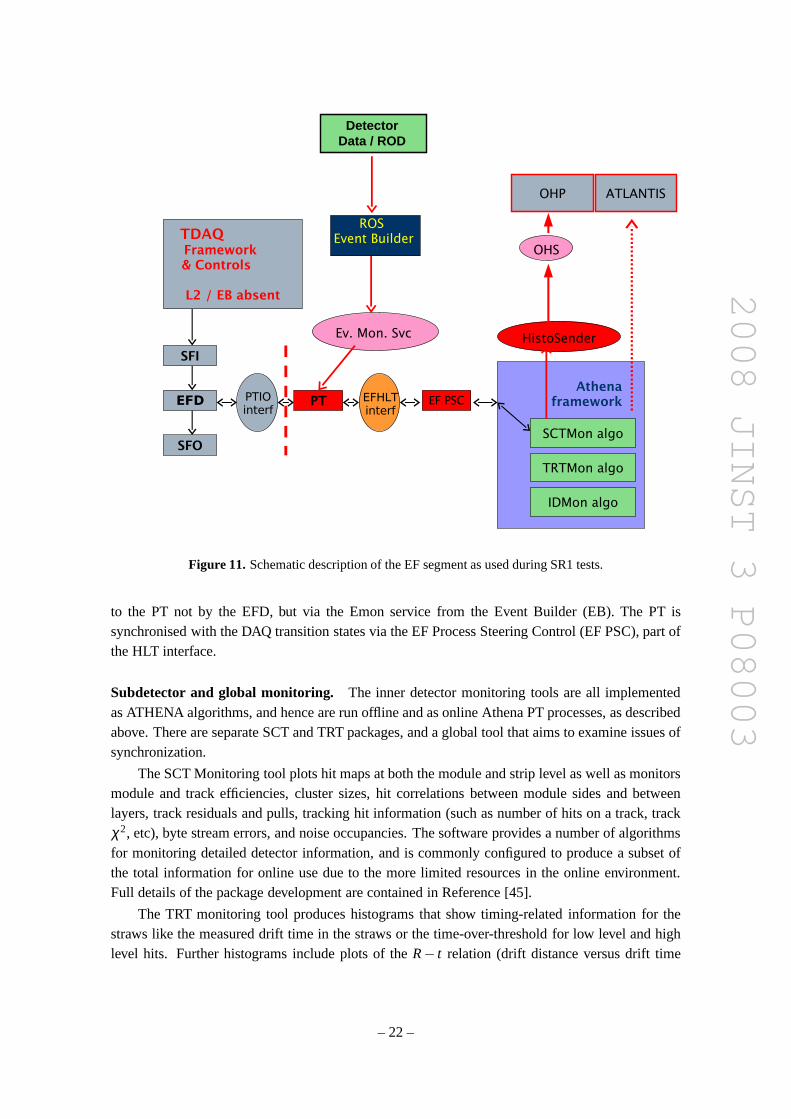
During SR1 commissioning, only a part of the ATLAS TDAQ system was in place, as shownin figure 11. In particular, there was no SFI during SR1 data taking, so that event data were passed
– 21 –
2008 JINST 3 P08003
DetectorData / ROD
Figure 11. Schematic description of the EF segment as used during SR1 tests.
to the PT not by the EFD, but via the Emon service from the EventBuilder (EB). The PT issynchronised with the DAQ transition states via the EF Process Steering Control (EF PSC), part ofthe HLT interface.
Subdetector and global monitoring. The inner detector monitoring tools are all implementedas ATHENA algorithms, and hence are run offline and as online Athena PT processes, as describedabove. There are separate SCT and TRT packages, and a global tool that aims to examine issues ofsynchronization.
The SCT Monitoring tool plots hit maps at both the module and strip level as well as monitorsmodule and track efficiencies, cluster sizes, hit correlations between module sides and betweenlayers, track residuals and pulls, tracking hit information (such as number of hits on a track, trackχ2, etc), byte stream errors, and noise occupancies. The software provides a number of algorithmsfor monitoring detailed detector information, and is commonly configured to produce a subset ofthe total information for online use due to the more limited resources in the online environment.Full details of the package development are contained in Reference [45].
The TRT monitoring tool produces histograms that show timing-related information for thestraws like the measured drift time in the straws or the time-over-threshold for low level and highlevel hits. Further histograms include plots of theR− t relation (drift distance versus drift time
– 22 –

2008 JINST 3 P08003
Figure 12. Difference between the SCT and TRT reconstructed trackφ parameter as a function of the eventnumber for one run of the combined barrel test. The synchronization between the readout of SCT and TRTsubdetectors was lost at event≈7600 and the run was stopped.
in the straw) for track hits, number of low-level and high level hits on a track as well as the trackresidual, which is the difference between measured and predicted hit positions. Another set ofhistograms monitors geometric quantities like the track’simpact parameter or its azimuthal angle.Additionally, various straw, noise, and track hitmaps are available.
The list of histograms produced by the global monitoring tool includes the synchronizationbetween the SCT and TRT readout, the∆φ of the perigee parameters of the SCT and TRT versusevent number (see, for example, figure 12), the mean number ofSCT and TRT segments, thenoise occupancy of the SCT and TRT, and the number of hits found on global tracks. Figure 12shows the difference of azimuth angle of track segments in the SCT and TRT versus event number,which is used to monitor the synchronization of readout between the subdetectors. It is clearlyvisible that the synchronization between the readout of SCTand TRT subdetectors was lost aroundevent 7600 and the run was stopped. The example shown in figure13 gives the variation of thenoise occupancy on the TRT Endcap C with the event number. In this case, the noise occupancyincreased from around 2% to 6% due to a trip of the analogue lowvoltage regulators. The globalmonitoring is also capable of extrapolating tracks from theSCT to the TRT in order to examine theTRT straw efficiencies.
3.4.2 SCT specialized monitoring
Most of the low level information about the SCT modules can beextracted directly from the bytestream file using an SCT standalone, monitoring program (sctComTool) with an event stream de-coder which unpacks the ROD fragments. As a result the hit strip numbers, trigger delay, andreadout errors are available. The byte stream has enough information to assign a hit to a module.
The low level monitoring includes occupancies at strip, chip, and module levels; dependencies
– 23 –

2008 JINST 3 P08003
0 2000 4000 6000 8000 10000 120000
0.01
0.02
0.03
0.04
0.05
0.06
0.07
0.08
0.09
0.1
TRT noise occupancy vs event number
Event number
TR
T N
oise
occ
upan
cy
Figure 13. TRT Endcap C noise occupancy as a function of the event number. A LV trip occurred aroundevent 1100.
of single and double hit8 occupancies on the trigger delay; and readout errors. A study of theoccupancy dependence on the trigger delay provides two types of results:
• If the trigger is random then the only recorded signals are due to noise. Different occupanciesat different trigger delays can indicate the presence of correlated noise with other subsystems.
• If the readout is triggered by real particles passing through the detector then the maximumoccupancy at certain trigger delay will indicate the right time for readout. The double hitoccupancy takes into account the position correlation between hits at both sides of a moduleand therefore such occupancy should give better noise background rejection. This leads tomore pronounced dependence of the double hit occupancy fromthe trigger delay.
The hits from tracks in the SCT will strongly bias the measured noise occupancy if these hitsare not subtracted. Therefore a special procedure was developed which determines the occupancyat module level on an event-by-event basis and subtracts thehits which were identified as belongingto space points.
3.4.3 TRT specialized monitoring
During the SR1 tests a TRT standalone monitoring tool (TRTViewer) was extensively used.TRTViewer runs at the ROD-Crate-DAQ (RCD) level and is a detector oriented tool which wasspecially developed as a flexible debugging and a fast diagnostics instrument. It is based on aROOT framework and contains some primitive tracking based on the least squares method, whichis necessary for the time tuning of the TRT parts and checks ofthe TRT basic functions.
The TRTViewer concept is based on the visualization of the basic detector characteristics ac-cording to the physical location of the elements: straws, chips, electronics boards, and detector
8A double hit is a coincidence between two sides of a module.
– 24 –
2008 JINST 3 P08003
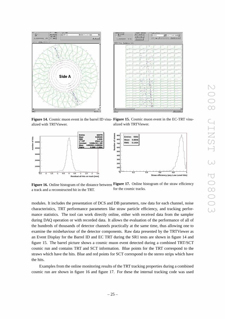
Figure 14. Cosmic muon event in the barrel ID visu-alized with TRTViewer.
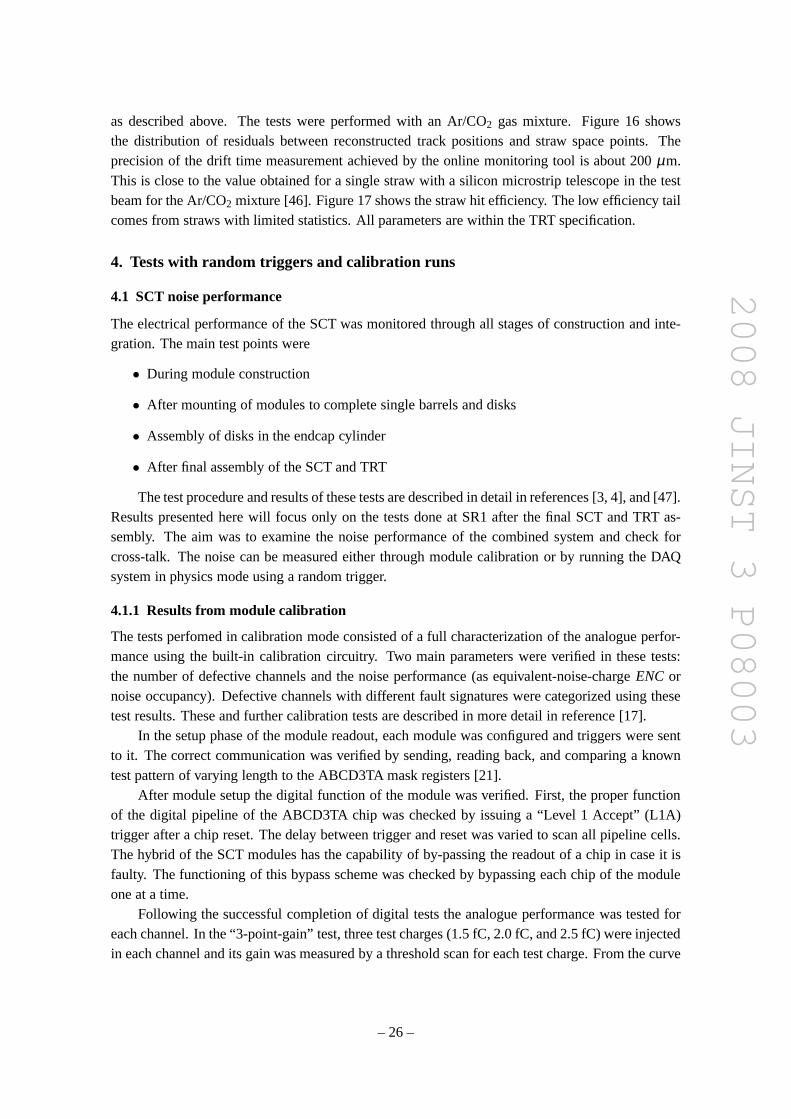
Figure 15. Cosmic muon event in the EC-TRT visu-alized with TRTViewer.
Entries 643779Mean 0.005103RMS 0.4106
/ ndf 2χ 376.9 / 11Constant 106± 5.546e+04 Mean 0.000334± 0.001916 Sigma 0.0004± 0.1968
-2.5 -2 -1.5 -1 -0.5 0 0.5 1 1.5 2 2.50
10000
20000
30000
40000
50000
Entries 643779Mean 0.005103RMS 0.4106
/ ndf 2χ 376.9 / 11Constant 106± 5.546e+04 Mean 0.000334± 0.001916 Sigma 0.0004± 0.1968
Residual all hits on track [mm]
num
ber
of h
its
Figure 16. Online histogram of the distance betweena track and a reconstructed hit in the TRT.
hTSEffiEntries 9302Mean 0.8846RMS 0.1434
0 0.2 0.4 0.6 0.8 10
100
200
300
400
500
600
700
800
900Entries 9302Mean 0.8846RMS 0.1434
Straw efficiency (any Low Level hits)
Num
ber
of s
traw
s
Figure 17. Online histogram of the straw efficiencyfor the cosmic tracks.
modules. It includes the presentation of DCS and DB parameters, raw data for each channel, noisecharacteristics, TRT performance parameters like straw particle efficiency, and tracking perfor-mance statistics. The tool can work directly online, eitherwith received data from the samplerduring DAQ operation or with recorded data. It allows the evaluation of the performance of all ofthe hundreds of thousands of detector channels practicallyat the same time, thus allowing one toexamine the misbehaviour of the detector components. Raw data presented by the TRTViewer asan Event Display for the Barrel ID and EC TRT during the SR1 tests are shown in figure 14 andfigure 15. The barrel picture shows a cosmic muon event detected during a combined TRT/SCTcosmic run and contains TRT and SCT information. Blue pointsfor the TRT correspond to thestraws which have the hits. Blue and red points for SCT correspond to the stereo strips which havethe hits.
Examples from the online monitoring results of the TRT tracking properties during a combinedcosmic run are shown in figure 16 and figure 17. For these the internal tracking code was used
– 25 –
2008 JINST 3 P08003
as described above. The tests were performed with an Ar/CO2 gas mixture. Figure 16 showsthe distribution of residuals between reconstructed trackpositions and straw space points. Theprecision of the drift time measurement achieved by the online monitoring tool is about 200µm.This is close to the value obtained for a single straw with a silicon microstrip telescope in the testbeam for the Ar/CO2 mixture [46]. Figure 17 shows the straw hit efficiency. The low efficiency tailcomes from straws with limited statistics. All parameters are within the TRT specification.
4. Tests with random triggers and calibration runs
4.1 SCT noise performance
The electrical performance of the SCT was monitored throughall stages of construction and inte-gration. The main test points were
• During module construction
• After mounting of modules to complete single barrels and disks
• Assembly of disks in the endcap cylinder
• After final assembly of the SCT and TRT
The test procedure and results of these tests are described in detail in references [3, 4], and [47].Results presented here will focus only on the tests done at SR1 after the final SCT and TRT as-sembly. The aim was to examine the noise performance of the combined system and check forcross-talk. The noise can be measured either through modulecalibration or by running the DAQsystem in physics mode using a random trigger.
4.1.1 Results from module calibration
The tests perfomed in calibration mode consisted of a full characterization of the analogue perfor-mance using the built-in calibration circuitry. Two main parameters were verified in these tests:the number of defective channels and the noise performance (as equivalent-noise-chargeENC ornoise occupancy). Defective channels with different faultsignatures were categorized using thesetest results. These and further calibration tests are described in more detail in reference [17].
In the setup phase of the module readout, each module was configured and triggers were sentto it. The correct communication was verified by sending, reading back, and comparing a knowntest pattern of varying length to the ABCD3TA mask registers[21].
After module setup the digital function of the module was verified. First, the proper functionof the digital pipeline of the ABCD3TA chip was checked by issuing a “Level 1 Accept” (L1A)trigger after a chip reset. The delay between trigger and reset was varied to scan all pipeline cells.The hybrid of the SCT modules has the capability of by-passing the readout of a chip in case it isfaulty. The functioning of this bypass scheme was checked bybypassing each chip of the moduleone at a time.
Following the successful completion of digital tests the analogue performance was tested foreach channel. In the “3-point-gain” test, three test charges (1.5 fC, 2.0 fC, and 2.5 fC) were injectedin each channel and its gain was measured by a threshold scan for each test charge. From the curve
– 26 –

2008 JINST 3 P08003
Mean 1680
RMS 74.69
ENC noise [e-]1400 1500 1600 1700 1800 1900 2000
num
ber
of c
hips
0
50
100
150
200
250 Mean 1680
RMS 74.69
Figure 18. Distribution of average equivalent noise charge (ENC) per readout chip for the SCT barrel sectorduring combined testing as measured by the SCT calibration.
of the threshold scan data, the gain was extracted as the threshold for 50% efficiency. A fit of acomplementary error function to the threshold scan yields the output noise at 2.0 fC, which wasused to extract the equivalent noise charge (ENC) as output noise divided by the channel gain.Figure 18 shows the average ENC noise per chip of the two sectors used in the combined tests. TheENC was measured at a hybrid operation temperature of around28 ◦C. The choice of temperaturewas driven by practical constraints of the test setup for dewpoint control. For final operation in theexperiment we envisage a hybrid temperature of≈0 ◦C, which will reduce the ENC noise [17].
With this noise test it was possible to identify defective channels (noisy or dead) as well asbonding defects (noise too high or low). The tests also allowed a comparison of the number of de-fective channels with results from earlier integration studies. No significant increase in the numberof bad channels was observed. From measurements carried outon single barrels and disks duringthe previous integration stage, we determined the percentage of defective channels as 0.2% in theSCT barrel and 0.3% in the SCT endcaps [17, 22].
The noise occupancy was measured with a threshold scan without charge injection. We definethe noise occupancy as the single channel noise occupancy per bunch-crossing. This strip noiseoccupancy is usually averaged over a readout chip (128 channels), or a module side (768 channels),or a full module (1536 channels). We quote the noise occupancy (number of noise hits per channeland L1A trigger) for a threshold of 1 fC, which will be the operational threshold in the experiment.The goal for the SCT is to have a noise occupancy of less than 5×10⁻⁴. Figure 19 shows the noiseoccupancy averaged over each chip of the two sectors used in the combined tests.
4.1.2 Results from random triggers
The noise tests performed in SR1 included runs at high trigger rates, tests of different groundingschemes, and tests of FE noise pickup during the active readout cycle of the TRT. In these tests the
– 27 –

2008 JINST 3 P08003
Mean 4.376e-05
RMS 2.629e-05
chip noise occupancy0 0.02 0.04 0.06 0.08 0.1 0.12 0.14
-310×
num
ber
of c
hips
0
10
20
30
40
50
60
70
80
90 Mean 4.376e-05
RMS 2.629e-05
Figure 19. Distribution of average noise occupancy per readout chip for the SCT barrel sector duringcombined testing as measured by the SCT calibration.
readout of the detectors was triggered by a pulser at fixed frequency or a pseudo-random trigger.Unless otherwise stated, the results shown here were obtained by running the ATHENA offlinecode on data that were taken with the SCT module thresholds set to 1.0 fC as given by the responsecurve calibration.
A simple illustration of the noise behaviour of the barrel SCT can be seen in figure 20, whichshows the strip number for all hits in the first 10000 events ofa run in which both the SCT and TRTwere powered and read out. The strip channel number goes from0 to 767, covering all strips onone side of a module. Hits from both sides of the module are therefore superimposed on the plot.The spikes represent the noisy strips present in the fraction of the SCT that was read out. Theyappear on a background of uniform noise.9 These nine noisy channels (out of a total of 718848)match those identified as problems in the calibration. Both subdetectors were triggered using apulse of 50 Hz and the thresholds of the SCT modules were set to1 fC. The expected modulationof the noise occupancy within a chip (128 channels) is also apparent in figure 20. The higher noisetoward the middle of the chip is due to power distribution inside the chip.
Several tests were performed in SR1 in order to investigate specific noise effects. These aresummarised below, and the results of the noise are given for each.
Trigger rate scan. For both the barrel and the endcap, physics mode runs were taken with dif-ferent trigger rates in order to check if this has any effect on the noise occupancy. The modulethresholds were set to 1 fC, and all other settings, such as the presence or absence of the TRT, werenot changed between runs.
Tables 4 and 5 contain a summary of the averaged noise occupancies measured for each layer
9In this sense, the plot shows the typical behaviour of a module side, with some smearing due to the cumulative effectof superimposing all module sides on the same plot.
– 28 –
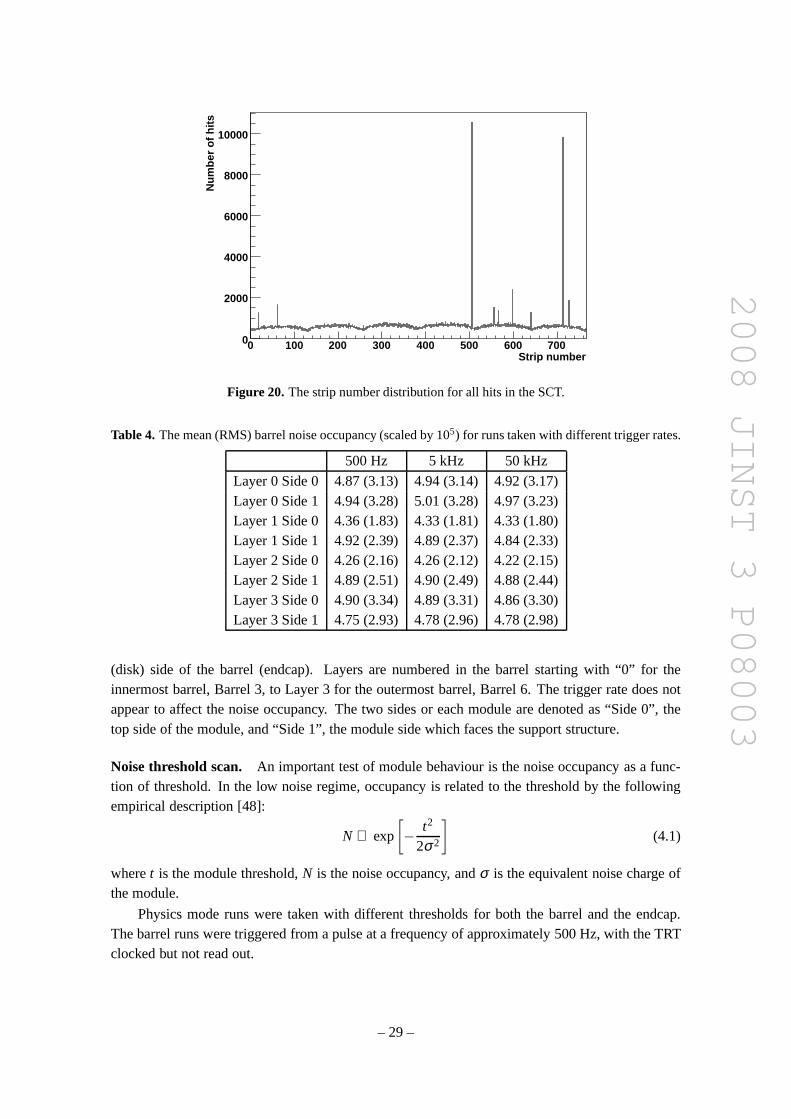
2008 JINST 3 P08003
Strip number0 100 200 300 400 500 600 7000
2000
4000
6000
8000
10000
Num
ber
of h
its
Figure 20. The strip number distribution for all hits in the SCT.
Table 4. The mean (RMS) barrel noise occupancy (scaled by 105) for runs taken with different trigger rates.
500 Hz 5 kHz 50 kHz
Layer 0 Side 0 4.87 (3.13) 4.94 (3.14) 4.92 (3.17)Layer 0 Side 1 4.94 (3.28) 5.01 (3.28) 4.97 (3.23)Layer 1 Side 0 4.36 (1.83) 4.33 (1.81) 4.33 (1.80)Layer 1 Side 1 4.92 (2.39) 4.89 (2.37) 4.84 (2.33)Layer 2 Side 0 4.26 (2.16) 4.26 (2.12) 4.22 (2.15)Layer 2 Side 1 4.89 (2.51) 4.90 (2.49) 4.88 (2.44)Layer 3 Side 0 4.90 (3.34) 4.89 (3.31) 4.86 (3.30)Layer 3 Side 1 4.75 (2.93) 4.78 (2.96) 4.78 (2.98)
(disk) side of the barrel (endcap). Layers are numbered in the barrel starting with “0” for theinnermost barrel, Barrel 3, to Layer 3 for the outermost barrel, Barrel 6. The trigger rate does notappear to affect the noise occupancy. The two sides or each module are denoted as “Side 0”, thetop side of the module, and “Side 1”, the module side which faces the support structure.
Noise threshold scan. An important test of module behaviour is the noise occupancyas a func-tion of threshold. In the low noise regime, occupancy is related to the threshold by the followingempirical description [48]:
N ∝ exp
[
− t2
2σ2
]
(4.1)
wheret is the module threshold,N is the noise occupancy, andσ is the equivalent noise charge ofthe module.
Physics mode runs were taken with different thresholds for both the barrel and the endcap.The barrel runs were triggered from a pulse at a frequency of approximately 500 Hz, with the TRTclocked but not read out.
– 29 –
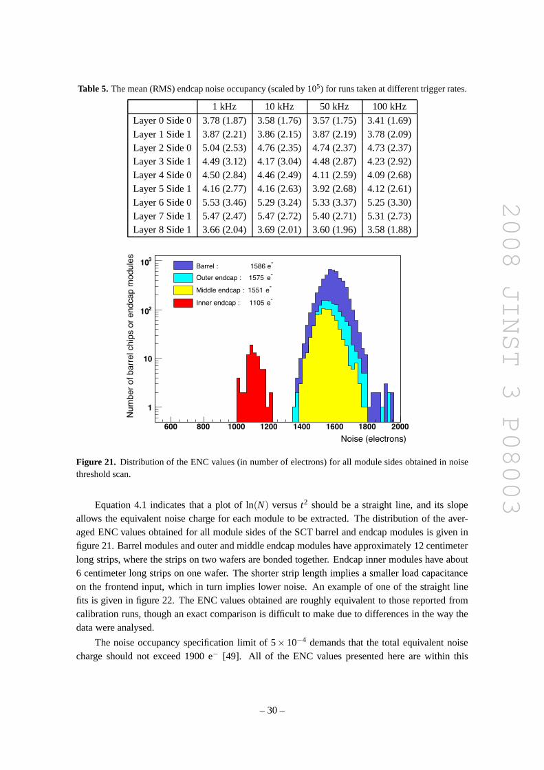
2008 JINST 3 P08003
Table 5. The mean (RMS) endcap noise occupancy (scaled by 105) for runs taken at different trigger rates.
1 kHz 10 kHz 50 kHz 100 kHz
Layer 0 Side 0 3.78 (1.87) 3.58 (1.76) 3.57 (1.75) 3.41 (1.69)Layer 1 Side 1 3.87 (2.21) 3.86 (2.15) 3.87 (2.19) 3.78 (2.09)Layer 2 Side 0 5.04 (2.53) 4.76 (2.35) 4.74 (2.37) 4.73 (2.37)Layer 3 Side 1 4.49 (3.12) 4.17 (3.04) 4.48 (2.87) 4.23 (2.92)Layer 4 Side 0 4.50 (2.84) 4.46 (2.49) 4.11 (2.59) 4.09 (2.68)Layer 5 Side 1 4.16 (2.77) 4.16 (2.63) 3.92 (2.68) 4.12 (2.61)Layer 6 Side 0 5.53 (3.46) 5.29 (3.24) 5.33 (3.37) 5.25 (3.30)Layer 7 Side 1 5.47 (2.47) 5.47 (2.72) 5.40 (2.71) 5.31 (2.73)Layer 8 Side 1 3.66 (2.04) 3.69 (2.01) 3.60 (1.96) 3.58 (1.88)
Noise (electrons)
600 800 1000 1200 1400 1600 1800 2000
Nu
mb
er
of
ba
rre
l ch
ips o
r e
nd
ca
p m
od
ule
s
1
10
210
310
Barrel : 1586 e-
Outer endcap : 1575 e-
Middle endcap : 1551 e-
Inner endcap : 1105 e-
Figure 21. Distribution of the ENC values (in number of electrons) for all module sides obtained in noisethreshold scan.
Equation 4.1 indicates that a plot of ln(N) versust2 should be a straight line, and its slopeallows the equivalent noise charge for each module to be extracted. The distribution of the aver-aged ENC values obtained for all module sides of the SCT barrel and endcap modules is given infigure 21. Barrel modules and outer and middle endcap moduleshave approximately 12 centimeterlong strips, where the strips on two wafers are bonded together. Endcap inner modules have about6 centimeter long strips on one wafer. The shorter strip length implies a smaller load capacitanceon the frontend input, which in turn implies lower noise. An example of one of the straight linefits is given in figure 22. The ENC values obtained are roughly equivalent to those reported fromcalibration runs, though an exact comparison is difficult tomake due to differences in the way thedata were analysed.
The noise occupancy specification limit of 5× 10⁻⁴ demands that the total equivalent noisecharge should not exceed 1900 e− [49]. All of the ENC values presented here are within this
– 30 –
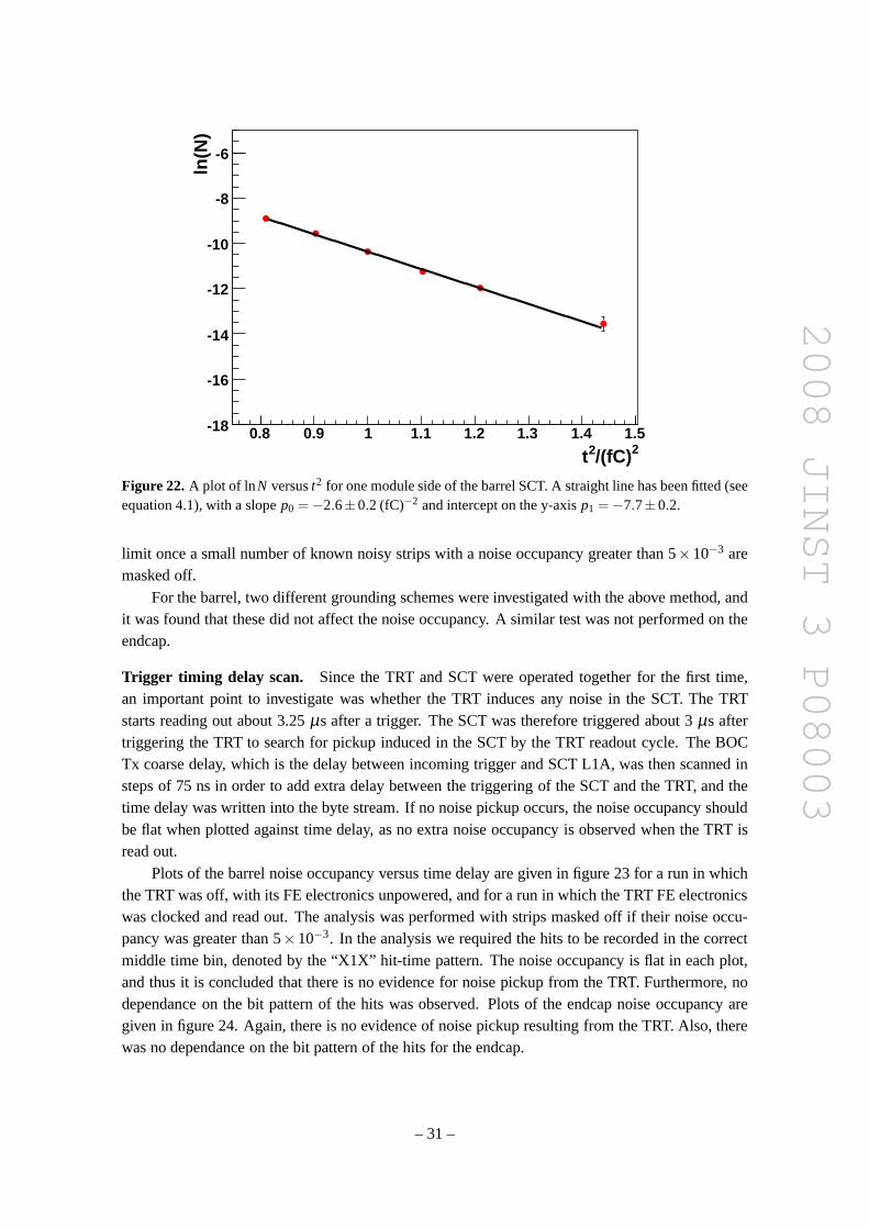
2008 JINST 3 P08003
0.8 0.9 1 1.1 1.2 1.3 1.4 1.5-18
-16
-14
-12
-10
-8
-6
2/(fC)2t
ln(N
)
Figure 22. A plot of lnN versust2 for one module side of the barrel SCT. A straight line has beenfitted (seeequation 4.1), with a slopep0 = −2.6±0.2 (fC)−2 and intercept on the y-axisp1 = −7.7±0.2.
limit once a small number of known noisy strips with a noise occupancy greater than 5×10⁻³ aremasked off.
For the barrel, two different grounding schemes were investigated with the above method, andit was found that these did not affect the noise occupancy. A similar test was not performed on theendcap.
Trigger timing delay scan. Since the TRT and SCT were operated together for the first time,an important point to investigate was whether the TRT induces any noise in the SCT. The TRTstarts reading out about 3.25µs after a trigger. The SCT was therefore triggered about 3µs aftertriggering the TRT to search for pickup induced in the SCT by the TRT readout cycle. The BOCTx coarse delay, which is the delay between incoming triggerand SCT L1A, was then scanned insteps of 75 ns in order to add extra delay between the triggering of the SCT and the TRT, and thetime delay was written into the byte stream. If no noise pickup occurs, the noise occupancy shouldbe flat when plotted against time delay, as no extra noise occupancy is observed when the TRT isread out.
Plots of the barrel noise occupancy versus time delay are given in figure 23 for a run in whichthe TRT was off, with its FE electronics unpowered, and for a run in which the TRT FE electronicswas clocked and read out. The analysis was performed with strips masked off if their noise occu-pancy was greater than 5×10⁻³. In the analysis we required the hits to be recorded in the correctmiddle time bin, denoted by the “X1X” hit-time pattern. The noise occupancy is flat in each plot,and thus it is concluded that there is no evidence for noise pickup from the TRT. Furthermore, nodependance on the bit pattern of the hits was observed. Plotsof the endcap noise occupancy aregiven in figure 24. Again, there is no evidence of noise pickupresulting from the TRT. Also, therewas no dependance on the bit pattern of the hits for the endcap.
– 31 –
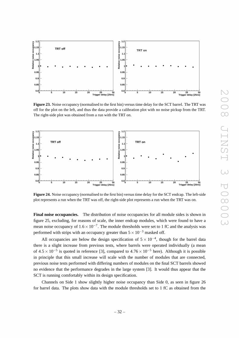
2008 JINST 3 P08003
Trigger delay [25ns]0 5 10 15 20 25 30
Rel
ativ
e no
ise
occu
panc
y
0.8
0.85
0.9
0.95
1
1.05
1.1
1.15
1.2
TRT off
0 5 10 15 20 25 30
Rel
ativ
e no
ise
occu
panc
y
0.8
0.85
0.9
0.95
1
1.05
1.1
1.15
1.2
TRT on
Trigger delay [25ns]
Figure 23. Noise occupancy (normalised to the first bin) versus time delay for the SCT barrel. The TRT wasoff for the plot on the left, and thus the data provide a calibration plot with no noise pickup from the TRT.The right-side plot was obtained from a run with the TRT on.
0 5 10 15 20 25 30
Rel
ativ
e no
ise
occu
panc
y
0.8
0.85
0.9
0.95
1
1.05
1.1
1.15
1.2
Trigger delay [25ns]
TRT off
0 5 10 15 20 25 30
Rel
ativ
e no
ise
occu
panc
y
0.8
0.85
0.9
0.95
1
1.05
1.1
1.15
1.2
Trigger delay [25ns]
TRT on
Figure 24.Noise occupancy (normalised to the first bin) versus time delay for the SCT endcap. The left-sideplot represents a run when the TRT was off, the right-side plot represents a run when the TRT was on.
Final noise occupancies. The distribution of noise occupancies for all module sides is shown infigure 25, excluding, for reasons of scale, the inner endcap modules, which were found to have amean noise occupancy of 1.6×10⁻⁷. The module thresholds were set to 1 fC and the analysis wasperformed with strips with an occupancy greater than 5×10⁻³ masked off.
All occupancies are below the design specification of 5× 10⁻⁴, though for the barrel datathere is a slight increase from previous tests, where barrels were operated individually (a meanof 4.5× 10⁻⁵ is quoted in reference [3], compared to 4.76× 10⁻⁵ here). Although it is possiblein principle that this small increase will scale with the number of modules that are connected,previous noise tests performed with differing numbers of modules on the final SCT barrels showedno evidence that the performance degrades in the large system [3]. It would thus appear that theSCT is running comfortably within its design specification.
Channels on Side 1 show slightly higher noise occupancy thanSide 0, as seen in figure 26for barrel data. The plots show data with the module thresholds set to 1 fC as obtained from the
– 32 –

2008 JINST 3 P08003
Noise occupancy0 0.05 0.1 0.15 0.2 0.25 0.3 0.35 0.4 0.45 0.5
-310×
Num
ber
of m
odul
e si
des
1
10
210Barrel: 4.7e-05
EC Outer: 5.2e-05
EC Middle: 3.8e-05
Figure 25. The distribution of noise occupancies for all module sides of the SCT detector, excluding theinner endcap modules.
Noise occupancy0 0.05 0.1 0.15 0.2 0.25 0.3 0.35 0.4 0.45 0.5
-310×
Num
ber
of m
odul
e si
des
0
10
20
30
40
50
Noise occupancy0 0.05 0.1 0.15 0.2 0.25 0.3 0.35 0.4 0.45 0.5
-310×
Num
ber
of m
odul
e si
des
0
10
20
30
40
50
Figure 26. The distribution of noise occupancies for the active modules of the SCT barrel detector for Side0 (left) and for Side 1 (right).
response curve calibration. The Side 0 distribution has a mean of 4.62× 10⁻⁵ and an RMS of2.70×10−5, while the Side 1 distribution has a mean of 4.90×10⁻⁵ and an RMS of 2.80×10⁻⁵.This is consistent with results obtained during module production.
4.2 TRT noise studies
Some of the most important issues during the combined tests were noise studies for different detec-tor configurations and different grounding schemes. Particular attention was given to the possibilityof inducing noise in the TRT from the SCT during combined operation.
TRT grounding and Faraday cage efficiency issues were addressed during standalone tests. Itwas found that a proper ground connection between the frontend boards and the Faraday cage isan important factor for the suppression of clock pickup noise. These connections must be made
– 33 –

2008 JINST 3 P08003
7A
7A
8A
8A
Figure 27. Noise occupancy map for the Barrel TRT sectors participating in the noise tests. Yellow colouredstraws have noise occupancies about 1.3% and black colouredstraws have noise occupancy above 4%.
with a spacing of not more than 3 cm to make a frequency cut at the level of above 100 MHz.After the implementation of this system, the noise level formost of the TRT channels was close tothat defined by thermal fluctuations. A typical picture of theTRT noise hit map for the modulesparticipating in the test is shown in figure 27. Yellow coloured straws have a noise occupancyof about 1.3% and black coloured straw have a noise occupancyabove 4%. One finds a groupof straws in the TRT module Type 1,10 which can be associated with one DTMROC chip witha systematically large noise occupancy. That is a known problem of these particular boards andis related to the board layout in which the 40 MHz clock line has a capacitive coupling with theASDBLR inputs. Details of the noise distribution across thechannels are shown in figure 28. Mostof the channels have noise at the level of 1%, but clock pickupaffected channels have noise levelsof up to 15%. Although that is a substantial noise level, it does not severely affect the physicsperformance.
A series of tests were performed to evaluate the change in TRTnoise during the combinedoperation of the SCT and TRT. The first test aimed to see the effect of SCT frontend power on TRTnoise occupancy. The noise occupancy differences for one ofthe TRT stacks (Stack 7) for sides Aand C are shown in figure 29. Positive values indicate an increase in noise between the reference(when the SCT was off) and when the SCT was on. Negative valuesindicate a decrease in noise.All deviations are within standard noise behaviour.
Following the ATLAS grounding convention, all detectors must have an independent groundconnection at one controlled point. In order to evaluate what happens if an uncontrolled groundshort appears during installation in the pit, a special testwas carried out. A worst case groundconnection was artificially created between the analogue ground plane in the TRT and the SCTpower return. A comparison of the TRT noise occupancy for this run with the reference one isshown in figure 30. No statistically significant effect was found during these tests.
A particular subject of interest was the effect of the SCT readout cycle on the TRT noise
10TRT barrel modules are stacked in layer with Type 1 modules forming the innermost layer, Type 2 modules the
– 34 –

2008 JINST 3 P08003
0 200 400 600 800 1000 1200 1400 16000
0.02
0.04
0.06
0.08
0.1
0.12
0.14
0.16
0.18
0.2
0.22
Straw number with any low level bit on
Occ
upan
cy
Figure 28. Noise occupancy distribution across the channels for one ofthe TRT Stacks (Stack 7 on Side A).Typical noise occupancy is about 1.3%.
Change in Occupancy (%)-10 -8 -6 -4 -2 0 2 4 6 8 10-110
1
10
210 Fit Mean = -0.01492Fit Sigma = 0.13945
Mean = -0.01253RMS = 0.19429
Stack7A - Change in Occupancy
Change in Occupancy (%)-10 -8 -6 -4 -2 0 2 4 6 8 10
-110
1
10
210
Stack7C - Change in Occupancy
Fit Mean = 0.03591Fit Sigma = 0.13050
Mean = 0.04354RMS = 0.24695
Stack7C - Change in Occupancy
Figure 29. Comparing noise occupancy when the SCT is off with a run when SCT is on. The horizontalaxis shows the difference of occupancy with SCT on minus occupancy with SCT off in percent. The verticalaxis gives the number of straws.
occupancy. Two types of tests were performed. In the first, TRT noise measurements were madeduring SCT operation at a trigger rate of 50 kHz. In order to increase SCT frontend digital activity,the SCT threshold was set to 0.8 fC. No change in the TRT noise occupancy was found. Anothertest aimed to look at exactly what happens during the SCT readout cycle. The time at whichthe SCT frontend chips transmit their header words to the backend corresponds to the maximumamount of frontend digital activity. Data were taken using different TRT delays with respect toSCT trigger. Figure 31 shows the typical occupancy difference with respect to the reference run.Again, no noticeable change was observed.
middle layer, and Type 3 modules the outermost layer.
– 35 –

2008 JINST 3 P08003
Change in Occupancy (%)-10 -8 -6 -4 -2 0 2 4 6 8 10-110
1
10
210 Fit Mean = -0.01025Fit Sigma = 0.12558
Mean = -0.01763RMS = 0.17109
Stack7A - Change in Occupancy
Change in Occupancy (%)-10 -8 -6 -4 -2 0 2 4 6 8 10
-110
1
10
210
Stack7C - Change in Occupancy
Fit Mean = -0.00512Fit Sigma = 0.12605
Mean = 0.00047RMS = 0.29187
Stack7C - Change in Occupancy
Figure 30. Comparison of the TRT noise occupancy when the TRT analogue ground plane is connected tothe SCT power return with the TRT standalone noise occupancy.
Change in Occupancy (%)-10 -8 -6 -4 -2 0 2 4 6 8 10-110
1
10
210 Fit Mean = 0.02258Fit Sigma = 0.19930
Mean = 0.06263RMS = 0.44481
Stack7A - Change in Occupancy
Change in Occupancy (%)-10 -8 -6 -4 -2 0 2 4 6 8 10
-110
1
10
210
Stack7C - Change in Occupancy
Fit Mean = 0.07140Fit Sigma = 0.20713
Mean = 0.09096RMS = 0.33160
Stack7C - Change in Occupancy
Figure 31. Comparison of the TRT noise occupancy during SCT readout cycle with the TRT standalonenoise occupancy.
5. Tests with cosmic triggers
5.1 Alignment and calibration
5.1.1 Alignment of the SCT and TRT
The determination of the position of the detector elements in space is crucial in order to make fulluse of the intrinsic resolution of the tracking device. The relative alignment of the sensors in amodule is given by the mounting precision during the module assembly [3], which used toleranceswell below the sensor spatial resolution. The mounting precision of modules on disks and barrels isless well known compared to the intrinsic resolution. This would lead to a significant degenerationof the tracking performance and needs to be corrected in the alignment step.
The position of the detector elements can be determined withtrack based alignment algo-rithms, based on the optimization of hit residuals. A perfectly aligned detector returns a residualdistribution centered around zero and with a width consistent with the quadratic sum of the in-trinsic resolution and the uncertainty originating from the track fit. A misaligned detector setupleads to a off-centered residual distribution with an increased width originating from the additionalmisalignment uncertainty.
– 36 –

2008 JINST 3 P08003
Track based alignment algorithms use the fact that the fit of the track trajectory is over-constrained and the deviations from the helix or the straight line in case of no magnetic field areminimized with respect to the translational and rotationaldegrees of freedom of the detector [50].Any deviation from the description of a perfect trajectory will appear as a misalignment of thedetector. Therefore the track selection processes for track based alignment use tracks with highmomentum to avoid kinks in the trajectory originating from multiple coulomb scattering (MCS)effects. As described above, the test setup was not inside a magnetic field. The momentum of thevarious charged particles could not be determined and no selection criteria based on the momen-tum could be applied. The momentum spectrum of particles from cosmic rays is dominated by lowmomentum particles, which suffer substantially from multiple scattering. The width of the resid-ual distribution, the quadratic sum of the intrinsic resolution, and the uncertainty from the trackreconstruction, is therefore dominated by multiple scattering. In particular, the impact of misalign-ment effects on the residual width is small compared to the multiple scattering effects. The trackfit algorithm normally applies the measured momentum to estimate the contribution from multiplescattering to the overall track position uncertainty. Since no momentum measurement is available,the uncertainty cannot be calculated and the multiple scattering contribution is set to zero. Thisleads to a significant underestimation of the uncertainty onthe track position.
The track based alignment approaches are based on the minimization of hit residuals. Thisis a necessary, but not sufficient requirement. The verticaltrack topology of the charged parti-cles originating from cosmic ray events can lead to degeneracies in the solution of the alignment,for example, a shearing of the detector in theYZ-plane cannot be recovered. In addition, verticalmovements along the track trajectory of the two shells are not constrained. These deformations,so calledweak modes, cannot be recovered by the alignment approaches. No track control sam-ple with a different track topology was available to verify the quality of the alignment constantsindependently. Therefore the conclusion on the obtained alignment constants is only limited.
Each SCT module has six degrees of freedom: three translations and three rotations. Thetranslation perpendicular to the strips is expected to be determined best. Overall for the SCT6×467= 2802 degrees of freedom have to be aligned. The TRT has no sensitivity along the wire,leading to five degrees of freedom per module times 12 TRT modules in the readout (overall 60degrees of freedom).
Several internal alignment approaches were developed and applied to data taken with the barrelSCT and the barrel TRT. The tracks used for the alignment werereconstructed using the standardATLAS reconstruction software framework ATHENA and the alignment algorithms were also im-plemented as a part of ATHENA.
5.1.2 Alignment of the SCT
Various alignment approaches were applied to align the SCT barrel in the SR1 cosmic setup [51 –54]. All approaches are based on the optimization of hit residuals. Figure 32 shows the residual dis-tribution for all modules located in a certain SCT layer obtained with the Globalχ2 approach [52].In this approach each module is aligned for six degrees of freedom. Modules with fewer than150 hits were kept stable. It is clearly visible that the residual distribution is distorted before thealignment corrections are applied. After the alignment themean for all layers is centered aroundzero and the width of the residual distribution is reduced compared to the width obtained with the
– 37 –

2008 JINST 3 P08003
residuals [mm]-0.3 -0.2 -0.1 0 0.1 0.2 0.3
num
ber
of h
its
0
1000
2000
3000
4000
5000
6000
7000SCT Layer 0
2 AlignedχGlobal
Nominal
residuals [mm]-0.3 -0.2 -0.1 0 0.1 0.2 0.3
num
ber
of h
its
0
1000
2000
3000
4000
5000
6000
7000
8000
9000 SCT Layer 1
2 AlignedχGlobal
Nominal
residuals [mm]-0.3 -0.2 -0.1 0 0.1 0.2 0.3
num
ber
of h
its
0
2000
4000
6000
8000
10000
12000
14000
SCT Layer 2
2 AlignedχGlobal
Nominal
residuals [mm]-0.3 -0.2 -0.1 0 0.1 0.2 0.3
num
ber
of h
its0
2000
4000
6000
8000
10000 SCT Layer 3
2 AlignedχGlobal
Nominal
Figure 32. The SCT biased residuals for the different layers of the SCT are shown before (red) and after(blue) the alignment.
misaligned setup. The other alignment approaches returnedsimilar results. As mentioned previ-ously, the width of the residuals distributions is dominated by multiple scattering and, in particular,effects due to detector misalignments might not be noticeable. In addition, the contribution to thetrack uncertainty originating from the track fit is largely underestimated, since the contributionfrom multiple scattering is not calculated.
All alignment algorithms used an iterative approach to get astable result. Figure 33 showsthe residual quantities as a function of iteration. The meanas well as the resolution of the residualdistribution converges to a stable number after three iterations. Convergence was reached when themovements of the detector were smaller than the corresponding statistical uncertainty. The initialshift of the mean was removed and the width of the resolutionσ got significantly smaller. Thewidth of the residuals varies between layers because the track error varies along the track, e.g., dueto multiple scattering.
The magnitude of the shifts obtained in the local X direction(orthogonal to the strip direction)is generally of the order of 100µm. The local Y alignment constants (along the strip direction) areof the order 600µm.
5.1.3 Comparison of alignment results with the photogrammetry measurements
Due to the fact that no magnetic field was used during SR1 data taking all tracks coming fromcosmic rays are straight lines. Thus, this setup was ideal todetermine the relative rotations of theSCT detector barrels inφ . A similar measurement was performed analysing the photogrammetrydata [56]. The first set of the three photogrammetry measurements, which was taken in November2005 [55], was precise enough to determine relative barrel rotations. However, these measurements
– 38 –
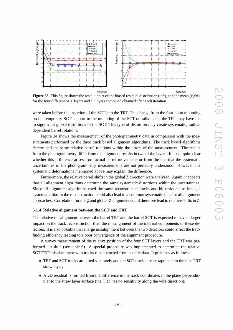
2008 JINST 3 P08003
Iteration
0 1 2 3 4 5 6 7 8
m)
µR
esid
ual s
igm
a (
0
10
20
30
40
50
60
70
80
90
100
Layer 0Layer 1Layer 2Layer 3All layers
Iteration
0 1 2 3 4 5 6 7 8
m)
µR
esid
ual m
ean
(
-15
-10
-5
0
5
10
15
Layer 0Layer 1Layer 2Layer 3All layers
Figure 33. This figure shows the resolutionσ of the biased residual distribution (left), and the mean (right),for the four different SCT layers and all layers combined obtained after each iteration.
were taken before the insertion of the SCT into the TRT. The change from the four point mountingon the temporary SCT support to the mounting of the SCT on rails inside the TRT may have ledto significant global distortions of the SCT. This type of distortion may create systematic, radius-dependent barrel rotations.
Figure 34 shows the measurement of the photogrammetry data in comparison with the mea-surements performed by the three track based alignment algorithms. The track based algorithmsdetermined the same relative barrel rotations within the errors of the measurement. The resultsfrom the photogrammetry differ from the alignment results in two of the layers. It is not quite clearwhether this difference arises from actual barrel movements or from the fact that the systematicuncertainties of the photogrammetry measurements are not perfectly understood. However, thesystematic deformations mentioned above may explain the difference.
Furthermore, the relative barrel shifts in the global Z direction were analysed. Again, it appearsthat all alignment algorithms determine the same systematic distortions within the uncertainties.Since all alignment algorithms used the same reconstructedtracks and hit residuals as input, asystematic bias in the reconstruction could also lead to a common systematic bias for all alignmentapproaches. Correlation for theφ and global-Z alignment could therefore lead to relative shifts in Z.
5.1.4 Relative alignment between the SCT and TRT
The relative misalignment between the barrel TRT and the barrel SCT is expected to have a largerimpact on the track reconstruction than the misalignment ofthe internal components of these de-tectors. It is also possible that a large misalignment between the two detectors could affect the trackfinding efficiency leading to a poor convergence of the alignment procedure.
A survey measurement of the relative position of the four SCTlayers and the TRT was per-formed “in situ” (see table 6). A special procedure was implemented to determine the relativeSCT-TRT misplacement with tracks reconstructed from cosmic data. It proceeds as follows:
• TRT and SCT tracks are fitted separately and the SCT tracks areextrapolated to the first TRTstraw layer;
• A 2D residual is formed from the difference in the track coordinates in the plane perpendic-ular to the straw layer surface (the TRT has no sensitivity along the wire direction);
– 39 –

2008 JINST 3 P08003
Layer0 0.5 1 1.5 2 2.5 3 3.5 4
Rot
atio
n [m
rad]
-0.25
-0.2
-0.15
-0.1
-0.05
0
0.05
0.1
0.15
0.2
0.25
Layer0 0.5 1 1.5 2 2.5 3 3.5 4
Shi
ft [m
m]
-0.25
-0.2
-0.15
-0.1
-0.05
0
0.05
0.1
0.15
0.2
0.25
Figure 34. For each SCT layer the relative rotation of the whole SCT barrel in φ is shown in mrad (left)and the relative Z shift in mm (right). Photogrammetry measurement are represented by green triangles,Robust Alignment results by blue circles, Localχ2 Alignment results by black squares, and Globalχ2
Alignment results by red squares. The alignment sets have been transformed into a common reference frameand normalised to layer 3.
Table 6. Relative translation and rotation between the SCT barrel and the TRT barrel as determined fromthe survey measurements.
∆x [mm] ∆y [mm] ∆rotX [mrad] ∆rotY [mrad]
-0.42 +0.33 +0.154 0.165
• A χ2 is constructed and minimized with similar techniques used in the alignment algorithms.Because of the SR1 setup (tracks almost vertical and no TRT sensitivity alongz) only themisplacement alongx (∆x) and the rotations around they (∆rotY) andz (∆rotZ) axes couldbe calculated.
This alignment procedure was applied to tracks collected from two different runs, one at the begin-ning and one at the end of a stable period of data taking. The two resulting SCT-TRT misalignmentvalues are consistent within their estimated uncertainties. Moreover, the track-based measurementsare found to be consistent with the survey measurements mentioned before.
5.1.5 Alignment of the TRT
After correcting for the relative alignment between the barrel SCT and TRT detectors, an internal
– 40 –

2008 JINST 3 P08003
x [mm]-1000 -500 0 500 1000
y [m
m]
-1000
-500
0
500
1000
translation x 2000
0.1 mm
translation x 2000
x [mm]-1000 -500 0 500 1000
y [m
m]
-1000
-500
0
500
1000rotation x 500
1 mrad
rotation x 500
Figure 35. Measured translations (left) and rotations (right) of TRT modules. The direction and size of thearrows in the left plot represent the direction and size of the translations. The rotation of the module in theright plot is proportional to the angle of the bar with the horizontal axis.
alignment of the TRT modules is carried out. In contrast to the SCT internal alignment described insection 5.1.2, where only SCT tracks were used, the TRT alignment employs extended SCT-TRTtracks. Since TRT tracks do not provide information outsidethexy-plane, SCT hits are needed toobtain thez coordinate of the track. Consequently, for a correct calculation of the TRT misalign-ment, the SCT modules need to be precisely aligned. A framework was developed to align TRTand SCT modules simultaneously and two of the approaches used in the SCT standalone align-ment (section 5.1.2) have been implemented in the framework. The result of this procedure is analignment that is consistent across both systems. The alignment constants obtained for the SCTare comparable, in terms of residuals, to the results from the other SCT alignment methods alreadypresented. Therefore, we will only report the TRT results.
The alignment of the TRT was limited to only the two most sensitive degrees of freedom,namely the direction perpendicular to the wire in the straw layer plane (∆X) and the rotation aroundthe wire axis (∆rotY).
The limited statistics and the nearly parallel track trajectories did not allow us to perform theTRT module alignment for the other weakly constrained degrees of freedom. The convergence ofthe alignment constants after successive iterations was reasonable, with the residual distributionscentered at zero after alignment. However, in contrast to the SCT case, the width of the TRTresidual distributions only marginally improved, due to the fact that for the TRT the alignmentcorrections are small (< 50 µm) with respect to the width of the residual distribution. Infigure 35the TRT module displacements returned by the alignment algorithm are shown graphically withthe values scaled for clarity. As can be seen, layer 0 and layer 2 modules are rotated in the samedirection while layer 1 modules are rotated in the opposite direction (both by approximately 300-400 µrad). Such a pattern is consistent with an elliptical distortion of the TRT (or possibly theSCT), but a conclusive interpretation cannot be obtained from the SR1 cosmic data.
A study of possible TRT module deformations was also carriedout. TRT module deviationsfrom the rigid body approximation are expected (caused by, for example, construction imperfec-
– 41 –
2008 JINST 3 P08003
tions, or mechanical stress) and if they are larger than the detector resolution, a correction mustbe applied. In terms of alignment, they effectively producea hit displacement depending on thehit position inside the module. Given the limited amount of available data, we limited our studyto the residual dependence on the hit position along the straw axis. Because the measurement ofthis coordinate is not provided by the TRT, it was derived by extrapolating SCT tracks to the TRTstraw layer under study (as a consequence, remaining alignment deviations in the SCT can alsoappear as module deformations in the TRT). For modules with larger statistics (layer 1 and layer 2)we actually observed significant deviations from zero. Somepatterns are consistent with moduletwists, others show more complicated deformations. A final conclusion on the magnitude of suchdeformations and their impact on track reconstruction willrequire more extensive data sets fromp-p collisions.
5.1.6 Alignment summary
Tracks reconstructed from cosmic ray events were used to determine the alignment of the barrelSCT, the barrel TRT, and the SCT with respect to the TRT. The calculated barrel alignment con-stants give a first indication as to the magnitude of the detector misalignments. The results forthe alignment are limited by multiple scattering of low momentum tracks. In addition the verticaltopology of the tracks from cosmic ray events leads toweak modesof the detector, which cannotbe resolved by track based alignment algorithms.
The three SCT alignment algorithms return consistent results. The magnitude of the shiftsin the local X direction is generally of the order 100µm. The local Y alignment constants areof the order 600µm. The comparison of the rotation around the global Z-coordinate betweenthe track based alignment and photogrammetry measurementsis not conclusive due to systematicuncertainties.
The alignment of the aligned SCT relative to the TRT is determined using tracks passingthrough both the SCT and the TRT. The alignment result is consistent with the survey measurementof the inner detector.
After the internal SCT alignment and the alignment of the SCTrelative to the TRT an internalalignment of TRT modules is performed. For this, SCT tracks extended to the TRT are used. Thevarious TRT modules move by about 50µm and are rotated by about 300 to 400µrad aroundthe wire axis. Internal deformations of the TRT modules are studied, but no final conclusion ispossible.
5.1.7 TRT drift time calibration
Drift time model. The TRT measures the drift time, the time between the LHC bunch clock andthe arrival of the signal to the anode wire, in time-to-digitcounts (TDC). A measured TDC value isa function of the position and orientation of the charged particle trajectory with respect to the driftcell. Since the TRT drift cells are symmetric around the wireaxis, the drift time is only a functionof the distance to the anode wire. The model used for calibration therefore reduces to:11
TDC(r) = α(tdrift(r)+ t0). (5.1)
11The propagation time and time-of-flight contributions werenot taken into account.
– 42 –
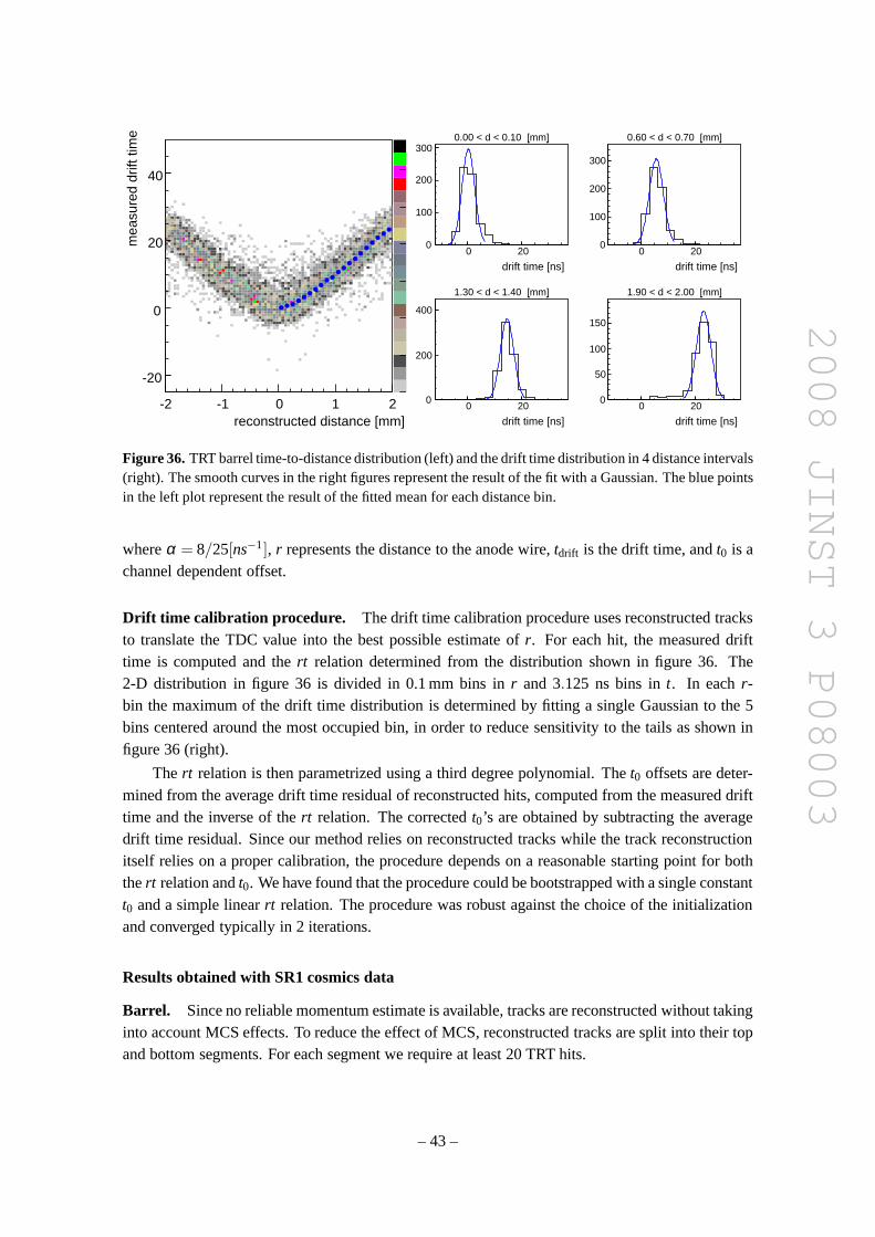
2008 JINST 3 P08003
reconstructed distance [mm]-2 -1 0 1 2
mea
sure
d dr
ift ti
me
-20
0
20
40
drift time [ns]0 20
0
100
200
3000.00 < d < 0.10 [mm]0.00 < d < 0.10 [mm]
drift time [ns]0 20
0
100
200
300
0.60 < d < 0.70 [mm]0.60 < d < 0.70 [mm]
drift time [ns]0 20
0
200
400
1.30 < d < 1.40 [mm]1.30 < d < 1.40 [mm]
drift time [ns]0 20
0
50
100
150
1.90 < d < 2.00 [mm]1.90 < d < 2.00 [mm]
Figure 36.TRT barrel time-to-distance distribution (left) and the drift time distribution in 4 distance intervals(right). The smooth curves in the right figures represent theresult of the fit with a Gaussian. The blue pointsin the left plot represent the result of the fitted mean for each distance bin.
whereα = 8/25[ns−1], r represents the distance to the anode wire,tdrift is the drift time, andt0 is achannel dependent offset.
Drift time calibration procedure. The drift time calibration procedure uses reconstructed tracksto translate the TDC value into the best possible estimate ofr. For each hit, the measured drifttime is computed and thert relation determined from the distribution shown in figure 36. The2-D distribution in figure 36 is divided in 0.1 mm bins inr and 3.125 ns bins int. In eachr-bin the maximum of the drift time distribution is determinedby fitting a single Gaussian to the 5bins centered around the most occupied bin, in order to reduce sensitivity to the tails as shown infigure 36 (right).
The rt relation is then parametrized using a third degree polynomial. Thet0 offsets are deter-mined from the average drift time residual of reconstructedhits, computed from the measured drifttime and the inverse of thert relation. The correctedt0’s are obtained by subtracting the averagedrift time residual. Since our method relies on reconstructed tracks while the track reconstructionitself relies on a proper calibration, the procedure depends on a reasonable starting point for boththert relation andt0. We have found that the procedure could be bootstrapped witha single constantt0 and a simple linearrt relation. The procedure was robust against the choice of theinitializationand converged typically in 2 iterations.
Results obtained with SR1 cosmics data
Barrel. Since no reliable momentum estimate is available, tracks are reconstructed without takinginto account MCS effects. To reduce the effect of MCS, reconstructed tracks are split into their topand bottom segments. For each segment we require at least 20 TRT hits.
– 43 –

2008 JINST 3 P08003
/ndof2χ
0 5 10 15 200
10000
20000
30000
/ndof2χ
0 5 10 15 20
wid
th o
f res
idua
l dis
trib
utio
n
0
0.5
1 from fit [-0.5,0.5]σ
rms [-2,2]
cut/ndof2χ
0 5 10 15 20
expe
cted
err
or o
n m
ean
0
0.05
0.1nu
mbe
r of
trac
ks
Figure 37. Distribution for χ2/ndof (left), width of the unbiased residual distribution inbins of χ2/ndof(centre), and estimate of the uncertainty on an estimate mean for a hypothetical set of 100 hits (right).
In the calibration procedure we require for each hit a time-over-threshold of at least 2×3.125 ns and a maximum time residual of 15 ns. The latter is chosen large, approximately 5 timesthe single hit resolution, to allow recovery from a poorly chosen starting value fort0 in the firstiteration. To improve the quality of the selected track segments, a cut is made on theχ2/ndof ofthe track. To prevent a bias in the calibration theχ2/ndof is first reduced by the contribution fromthe selected hit. The resultingχ2/ndof distribution is shown in figure 37.
The centre plot in figure 37 shows the width of the unbiased residual distribution in binsχ2/ndof. The width is measured both as an RMS on the interval±2 mm and as theσ of a Gaussianfit on the interval±0.5 mm. The latter result shows that a single hit resolution of around 200µm isobtained.
To motivate the choice of a particularχ2/ndof selection we calculate the uncertainty on themean of the residual distribution as a function of theχ2/ndof cut. The uncertainty is estimatedasσ(mean) = RMS/
√N−1. The rightmost plot in figure 37 shows the result, normalised for a
hypothetical set of 100 hits. As one can see contribution from hits with χ2/ndof > 10 actuallydegrades the resolution on the mean.12 Therefore only hits for whichχ2/ndof is smaller than 10are selected in order to reach an optimal sensitivity for calibration. Although this may seem tobe an unrealistically large value, it already rejects a significant fraction of the segments becausemultiple scattering effects are ignored.
For the cosmics data we use a singlert relation for all straws. The drift time offsett0 isdetermined for each straw separately. The uncertainty in the t0 is the RMS of the drift time residualdistribution divided by the square root of the number of entries (minus 1). Since the RMS of thedrittime residual distribution is itself proportional to the resolution, the fractional contribution ofthe uncertainty int0 to the hit resolution is about
√
1+1/N−1≈ 1/2N. To keep this contributionbelow 1% one would need about 50 hits per straw. For the calibration of the cosmics data we haverequired a minimum of 25 hits, based on considerations discussed below. For straws not fullfilingthe above requirements, we use the average value of thet0 of the corresponding TRT module as acompromise between the statistical and systematic uncertainties.
It is generally assumed that the time offsets of straws within one “DTMROC” unit (16 straws
12The reason that welosesensitivity, even though weadd information is that in the extraction of the mean we do notuse the fact that the uncertainty varies withχ2/ndof.
– 44 –
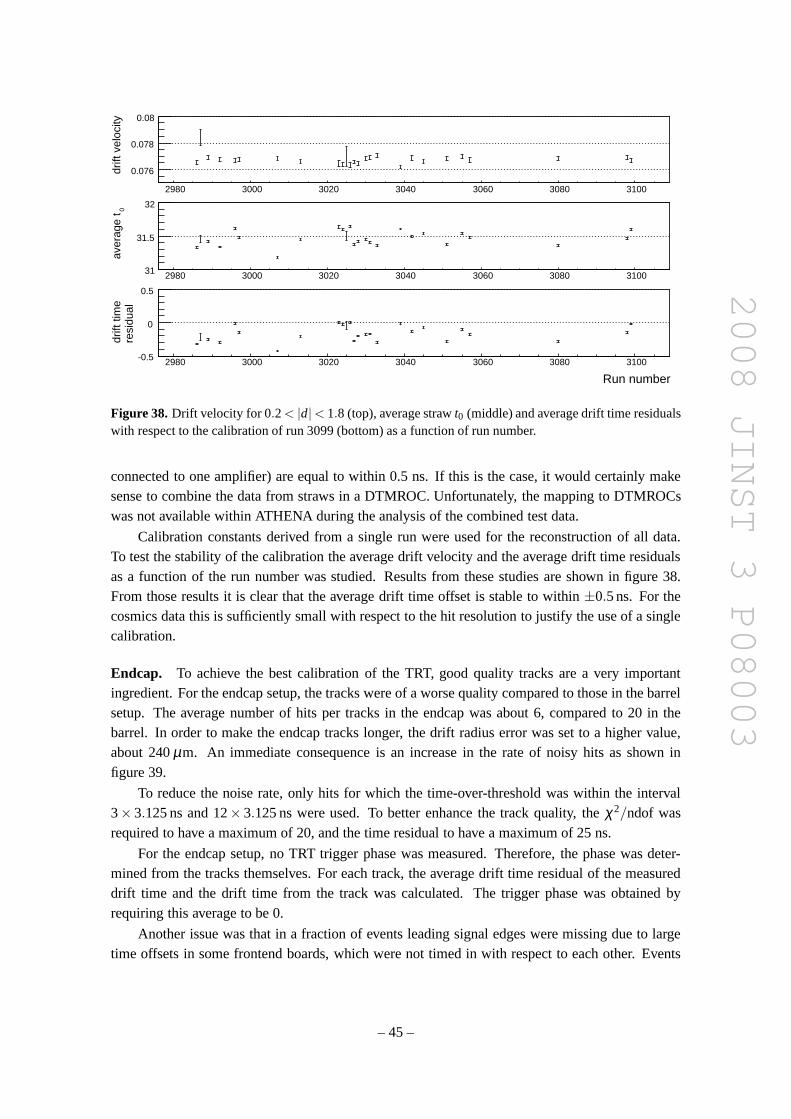
2008 JINST 3 P08003
2980 3000 3020 3040 3060 3080 3100
drift
vel
ocity
0.076
0.078
0.08
2980 3000 3020 3040 3060 3080 3100
aver
age
t 0
31
31.5
32
2980 3000 3020 3040 3060 3080 3100
Run number
drift
tim
ere
sidu
al
-0.5
0
0.5
Figure 38. Drift velocity for 0.2< |d|< 1.8 (top), average strawt0 (middle) and average drift time residualswith respect to the calibration of run 3099 (bottom) as a function of run number.
connected to one amplifier) are equal to within 0.5 ns. If thisis the case, it would certainly makesense to combine the data from straws in a DTMROC. Unfortunately, the mapping to DTMROCswas not available within ATHENA during the analysis of the combined test data.
Calibration constants derived from a single run were used for the reconstruction of all data.To test the stability of the calibration the average drift velocity and the average drift time residualsas a function of the run number was studied. Results from these studies are shown in figure 38.From those results it is clear that the average drift time offset is stable to within±0.5 ns. For thecosmics data this is sufficiently small with respect to the hit resolution to justify the use of a singlecalibration.
Endcap. To achieve the best calibration of the TRT, good quality tracks are a very importantingredient. For the endcap setup, the tracks were of a worse quality compared to those in the barrelsetup. The average number of hits per tracks in the endcap wasabout 6, compared to 20 in thebarrel. In order to make the endcap tracks longer, the drift radius error was set to a higher value,about 240µm. An immediate consequence is an increase in the rate of noisy hits as shown infigure 39.
To reduce the noise rate, only hits for which the time-over-threshold was within the interval3× 3.125 ns and 12× 3.125 ns were used. To better enhance the track quality, theχ2/ndof wasrequired to have a maximum of 20, and the time residual to havea maximum of 25 ns.
For the endcap setup, no TRT trigger phase was measured. Therefore, the phase was deter-mined from the tracks themselves. For each track, the average drift time residual of the measureddrift time and the drift time from the track was calculated. The trigger phase was obtained byrequiring this average to be 0.
Another issue was that in a fraction of events leading signaledges were missing due to largetime offsets in some frontend boards, which were not timed inwith respect to each other. Events
– 45 –
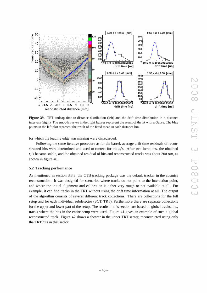
2008 JINST 3 P08003
reconstructed distance [mm]-2 -1.5 -1 -0.5 0 0.5 1 1.5 2
mea
sure
d dr
ift ti
me
-20
-10
0
10
20
30
40
50
0
20
40
60
80
100
120
drift time [ns]-10-5 0 5 1015202530350
100200300400500600700800900
0.00 < d < 0.10 [mm]
drift time [ns]-10-5 0 5 10 1520 2530350
200
400
600
800
1000
12000.60 < d < 0.70 [mm]
drift time [ns]-10-5 0 5 1015202530350
200
400
600
800
1000
1.30 < d < 1.40 [mm]
drift time [ns]-10-5 0 5 10 1520 2530350
50100150200250300350400450
1.90 < d < 2.00 [mm]
Figure 39. TRT endcap time-to-distance distribution (left) and the drift time distribution in 4 distanceintervals (right). The smooth curves in the right figures represent the result of the fit with a Gauss. The bluepoints in the left plot represent the result of the fitted meanin each distance bin.
for which the leading edge was missing were disregarded.Following the same iterative procedure as for the barrel, average drift time residuals of recon-
structed hits were determined and used to correct for thet0’s. After two iterations, the obtainedt0’s became stable, and the obtained residual of hits and reconstructed tracks was about 200µm, asshown in figure 40.
5.2 Tracking performance
As mentioned in section 3.3.3, the CTB tracking package was the default tracker in the cosmicsreconstruction. It was designed for scenarios where tracksdo not point to the interaction point,and where the initial alignment and calibration is either very rough or not available at all. Forexample, it can find tracks in the TRT without using the drift time information at all. The outputof the algorithm consists of several different track collections. There are collections for the fullsetup and for each individual subdetector (SCT, TRT). Furthermore there are separate collectionsfor the upper and lower part of the setup. The results in this section are based on global tracks, i.e.,tracks where the hits in the entire setup were used. Figure 41gives an example of such a globalreconstructed track. Figure 42 shows a shower in the upper TRT sector, reconstructed using onlythe TRT hits in that sector.
– 46 –

2008 JINST 3 P08003
/ ndf 2χ 313.8 / 3
cnstnt 62.2± 8020
mean 0.001439± 0.001242
sigma 0.0020± 0.1997
Residual (mm)-5 -4 -3 -2 -1 0 1 2 3 4 50
1000
2000
3000
4000
5000
6000
7000
8000 / ndf 2χ 313.8 / 3
cnstnt 62.2± 8020
mean 0.001439± 0.001242
sigma 0.0020± 0.1997 nu
mbe
r of
hits
Figure 40. Residual of reconstructed hits obtained after two iterations.
ATLAS Atlantis 2006-06-02 17:45:23 MET DST Event: JiveXML_2850_00023 Run: 2850 Event: 23
-100 1000 X (cm)
-100
100
0Y
(cm
)
Figure 41. A reconstructed cosmic track with both SCT and TRT hits.
– 47 –
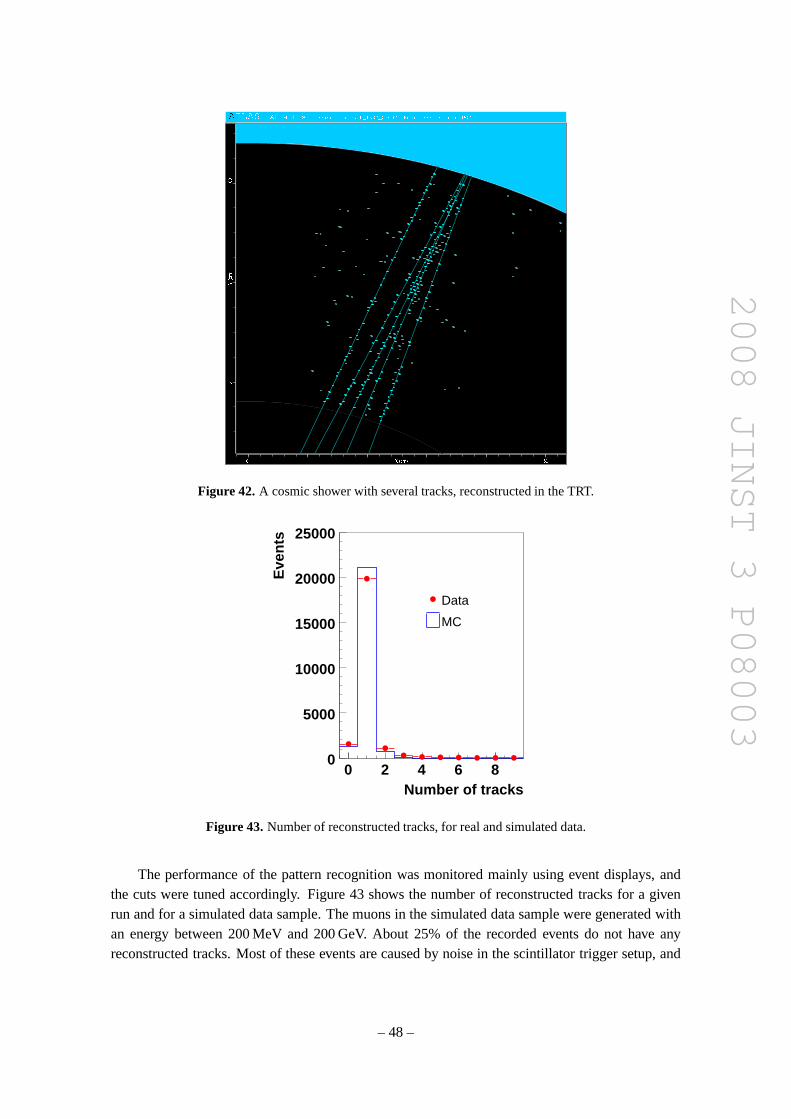
2008 JINST 3 P08003
Figure 42. A cosmic shower with several tracks, reconstructed in the TRT.
Number of tracks0 2 4 6 8
Eve
nts
0
5000
10000
15000
20000
25000
Data
MC
Figure 43. Number of reconstructed tracks, for real and simulated data.
The performance of the pattern recognition was monitored mainly using event displays, andthe cuts were tuned accordingly. Figure 43 shows the number of reconstructed tracks for a givenrun and for a simulated data sample. The muons in the simulated data sample were generated withan energy between 200 MeV and 200 GeV. About 25% of the recorded events do not have anyreconstructed tracks. Most of these events are caused by noise in the scintillator trigger setup, and
– 48 –
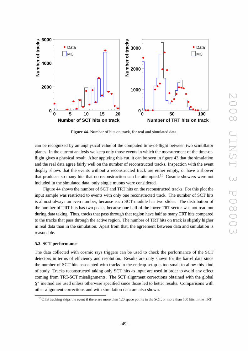
2008 JINST 3 P08003
Number of SCT hits on track0 5 10 15 20
Num
ber
of tr
acks
0
2000
4000
6000
Data
MC
Number of TRT hits on track0 50 100
Num
ber
of tr
acks
0
1000
2000
3000 Data
MC
Figure 44. Number of hits on track, for real and simulated data.
can be recognized by an unphysical value of the computed time-of-flight between two scintillatorplanes. In the current analysis we keep only those events in which the measurement of the time-of-flight gives a physical result. After applying this cut, it can be seen in figure 43 that the simulationand the real data agree fairly well on the number of reconstructed tracks. Inspection with the eventdisplay shows that the events without a reconstructed trackare either empty, or have a showerthat produces so many hits that no reconstruction can be attempted.13 Cosmic showers were notincluded in the simulated data, only single muons were considered.
Figure 44 shows the number of SCT and TRT hits on the reconstructed tracks. For this plot theinput sample was restricted to events with only one reconstructed track. The number of SCT hitsis almost always an even number, because each SCT module has two slides. The distribution ofthe number of TRT hits has two peaks, because one half of the lower TRT sector was not read outduring data taking. Thus, tracks that pass through that region have half as many TRT hits comparedto the tracks that pass through the active region. The numberof TRT hits on track is slightly higherin real data than in the simulation. Apart from that, the agreement between data and simulation isreasonable.
5.3 SCT performance
The data collected with cosmic rays triggers can be used to check the performance of the SCTdetectors in terms of efficiency and resolution. Results areonly shown for the barrel data sincethe number of SCT hits associated with tracks in the endcap setup is too small to allow this kindof study. Tracks reconstructed taking only SCT hits as inputare used in order to avoid any effectcoming from TRT-SCT misalignments. The SCT alignment corrections obtained with the globalχ2 method are used unless otherwise specified since those led tobetter results. Comparisons withother alignment corrections and with simulation data are also shown.
13CTB tracking skips the event if there are more than 120 space points in the SCT, or more than 500 hits in the TRT.
– 49 –

2008 JINST 3 P08003
Hit pattern000
001
010
011
100
101
110
111
Ent
ries/
hit p
atte
rn
0
50
100
150
200
250
300
350
400
450
310×
Figure 45. SCT hit pattern.
5.3.1 Timing
The SCT was run in the expanded mode in the cosmic runs, which provides time information forthe triggered time bin as well as the preceding and followingbins. Figure 45 shows the distributionof the hit patterns for a given run. The 010 hit pattern is dominant, indicating that the trigger istimed well with respect to the SCT modules. The 20 ns shaping time of the ABCD3TA chip willalso give rise to hits in adjacent time bins as the pulse duration above threshold can be longer thanthe 25ns bunch-crossing time window. Hit pattern 001 comes from cases where the hit is registeredin the next time bin due to a muon arriving late in the clock cycle. The majority of hits in eachevent are noise hits, and thus not correlated with the trigger. Notice that there are also some hitswith the hit pattern 000. As the readout chip should only output hits from fired channels, this is nota valid hit pattern. Three modules showed this phenomenon inthe tests at SR1, on a whole module,on a chip, and on a single channel, respectively.
5.3.2 Efficiency
The efficiency of a given SCT module side was computed using the following method. For eachreconstructed track in an event that remains after a qualitycut, the algorithm removed any hitslocated on the SCT barrel layer under investigation, or theith layer. A track refit was then performedexcluding these hits. From the perigee parameters of this new track, an extrapolation to theith layerwas performed to obtain the intersection point or “predicted position” of a hit on a module. If thisintersection point was within the sensitive area of the module it was included in the denominatorof the efficiency calculation. If a SCT cluster was found to belocated within a set distance fromthe predicted position, an entry was made for the numerator.
Various track quality cuts and fiduciality requirements were made before a hit prediction en-tered the denominator of the efficiency calculation:
• the track must have 10 or more SCT hits
• the track fit must have aχ2/ndof≤ 24
– 50 –

2008 JINST 3 P08003
layer and side0 0.5 1 1.5 2 2.5 3 3.5 4
0.98
0.982
0.984
0.986
0.988
0.99
0.992
0.994
0.996
0.998
1
Unb
iase
d H
it E
ffici
ency
2mm roadwidth
1.5mm roadwidth
1.0mm roadwidth
0.5mm roadwidth
99% eff
Figure 46. The hit efficiency for the different barrel layers and sides from simulated cosmic data withpT
greater than 200 MeV. Also shown is the specification efficiency of 99% (dashed blue line).
• the track must have an incidence angle on the module of less than 20 degrees in the azimuthaldirection
• the track intersection point on the module must be at least 2 mm from the bond gap and 1.5mm from the edges of the module
• the track intersection point must be at least 1.5 mm from any masked strips or chips
In order for a hit to be entered into the numerator of the efficiency calculation, in addition tothe above requirements, a hit must be found within a certain road width around the predicted hitposition. By default, and unless specified otherwise, this road width was 2 mm.
In order to choose a proper value for the cut applied to the distance from the predicted trackposition and the cluster position, the simulation was used.Due to the lack of magnetic field, thisdistance can be quite large for tracks corresponding to low momentum cosmic rays. Figure 46shows the average efficiency per SCT layer, for different distance cuts, for all simulated particles.In order to neglect MCS effects, a cut of 2 mm was then chosen tocompute efficiencies from realdata. The result obtained in this case is shown in figure 47, where after alignment the unbiased hitefficiency in all barrel layers is measured to be within specifications, i.e., greater than 99%.
Since the cosmic trigger is not synchronized with the readout clock, the collected data canalso be used to study the dependence of the SCT efficiency withthe arrival time of the particle withrespect to the readout time. This difference in time was measured and since the SCT is recordingthe information of three consecutive bunch crossings, the measurement can be done over a timerange of 75 ns. Figure 48 shows the SCT efficiency obtained in the barrel section as a functionof the arrival time of the particle. The efficiency remains high for a range of 4 ns, compared to
– 51 –
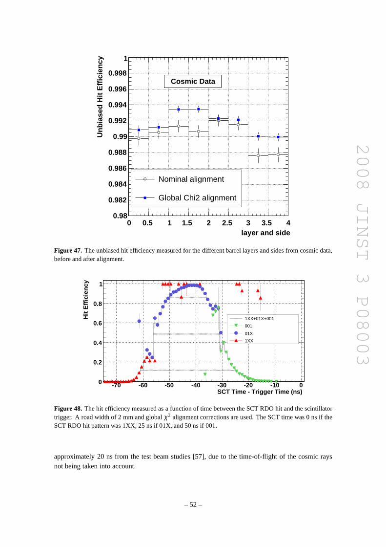
2008 JINST 3 P08003
layer and side0 0.5 1 1.5 2 2.5 3 3.5 4
Unb
iase
d H
it E
ffici
ency
0.98
0.982
0.984
0.986
0.988
0.99
0.992
0.994
0.996
0.998
1
Nominal alignment
Global Chi2 alignment
Cosmic Data
Figure 47. The unbiased hit efficiency measured for the different barrel layers and sides from cosmic data,before and after alignment.
SCT Time - Trigger Time (ns)-70 -60 -50 -40 -30 -20 -10 0
Hit
Effi
cien
cy
0
0.2
0.4
0.6
0.8
1
1XX+01X+001
001
01X
1XX
Figure 48. The hit efficiency measured as a function of time between the SCT RDO hit and the scintillatortrigger. A road width of 2 mm and globalχ2 alignment corrections are used. The SCT time was 0 ns if theSCT RDO hit pattern was 1XX, 25 ns if 01X, and 50 ns if 001.
approximately 20 ns from the test beam studies [57], due to the time-of-flight of the cosmic raysnot being taken into account.
– 52 –

2008 JINST 3 P08003
layer and side0 0.5 1 1.5 2 2.5 3 3.5 4
aver
age
Res
idua
l mea
n [m
m]
-0.003
-0.002
-0.001
0
0.001
0.002
0.003
layer and side0 0.5 1 1.5 2 2.5 3 3.5 4
aver
age
Res
idua
l sig
ma
[mm
]
00.010.020.030.040.050.060.070.080.090.1
Figure 49. The unbiased residual means for the different layers and sides of the SCT modules for simulation(triangle) and data using globalχ2 alignment (squares). A road width of 2 mm is used.
5.3.3 SCT resolution
The SCT detector resolution can be extracted from theσ of the SCT residual distribution of a givenmodule side after subtracting the track prediction and alignment corrections uncertainties. How-ever, as mentioned above, the track uncertainty is not well estimated for the case of low momentumparticles. Figure 49 shows the mean andσ of the unbiased residuals measured for data (usingglobal χ2 alignment constants) and Monte Carlo simulation. For both the data and simulation themeasured residuals are much larger than the expected detector resolution of 23µm due to the effectof multiple scattering.
Figure 50 shows for simulated data theσ of the SCT residual and pull distribution as a functionof the true particle energy. Theσ of the residual distribution increases for low energy tracks andfor this case theσ of the residual pull distribution is no longer 1 due to the already mentionedwrong track uncertainty estimation. For high momentum tracks, aσ of around 28µm is obtained.After subtracting in quadrature the track uncertainty contribution (which is estimated to be around16 µm), a value of 23µm is obtained in agreement with the intrinsic detector resolution.
In order to determine the detector resolution from the data,the σ of the residual distributionas a function of the unbiased trackχ2 (i.e., removing the contribution to theχ2 of the hit underevaluation) was measured, for side 1 of modules in layer 2. These modules were chosen to max-imise statistics, and minimize track errors. The result obtained is shown in figure 51 for real and
– 53 –

2008 JINST 3 P08003
E [MeV]0 2000 4000 6000 8000 10000 12000 14000 16000 18000 20000
[mm
]σ
0.02
0.03
0.04
0.05
0.06
0.07
0.08
0.09
0.1
0.11
SCT Resolution as a function of energy
E [MeV]0 2000 4000 6000 8000 10000 12000 14000 16000 18000 20000
[mm
]σ
1
1.5
2
2.5
3
3.5
SCT pulls as a function of energy
Figure 50. σ of SCT unbiased residuals (left) and pull distributions (right) as a function of true particleenergy.
0 1 2 3 4 5 6 7 8 9
Res
idua
l Sig
ma
(mm
)
0
0.02
0.04
0.06
0.08
0.1
0.12data
MC
Figure 51. Width of the SCT unbiased residuals, as a function of the unbiased trackχ2 per number ofdegrees of freedom, for real and simulated cosmic data.
simulated data. When theχ2 tends to zero, the contribution of low momentum tracks should benegligible. Aσ of 24± 1 µm (20± 2 µm) is obtained for real (simulated) data for tracks with aχ2
per degrees of freedom of less than 1. For these tracks the contribution to the residual from trackuncertainty is negligable. Alignment uncertainties have not been considered resulting in slightlylarger residuals in real data than in simulation. The low measured residuals are due to the largenumber of double clusters present in both data and simulation. Approximately one in three of theclusters in the SCT is a two hit cluster, in both data and simulation. This means that most tracksintercepting the module near the edge of the strip will produce two strip clusters. This effectivelyreduces the resolution of the one-strip cluster measurement.
– 54 –
2008 JINST 3 P08003
5.4 TRT performance
5.4.1 TRT efficiency
The data collected in the SR1 test were also used to study the efficiency of the TRT straw tubes.Because of the limited statistics in the endcap, this study was only performed for the barrel.
It is important to note that, given the lack of track momentuminformation, an accurate mea-surement of the straw efficiency with cosmic data is difficult. Multiple scattering effects cannot beaccounted for and hence there is a high uncertainty on the relative position of the passing particlewith respect to the straw tubes. On the other hand, knowing whether a particle passes through theactive region of a straw or not, is essential in determining its efficiency.
For this reason particular care was devoted to selection of tracks for this study in order toreduce the uncertainties resulting from multiple scattering. The detector geometry was correctedusing the procedure described in section 5.1.5 for simultaneously aligning the SCT and TRT.
The track selection proceeded as follows:
• Full SCT+TRT tracks were reconstructed and, to suppress events generated by cosmic show-ers, only events with a single track were selected,
• SCT track segments from the top and bottom sectors were combined and the resulting SCTtracks were required to be of high quality (χ2/ndof< 5),
• SCT tracks were extrapolated to the TRT. The distance between the extrapolated track inter-section at the last straw layer (corresponding to the maximum lever arm) and the closest hitin the same straw layer was required to be less than 0.3 mm.
Monte Carlo studies have shown that this selection procedure reduces the presence of tracksat the low end of the momentum spectrum. These tracks are mostaffected by multiple scattering.Most importantly, no requirements were made on the quality of the TRT segments themselves, inparticular no cuts were applied to theχ2 of the TRT (or SCT+TRT) tracks. In this way the biason the efficiency induced by the track selection is kept to a minimum for layers other than the laststraw layer.
For each straw the efficiency was defined as the ratio between the number of “expected” hits(i.e., the number of tracks passing closer than a certain distanceR to the straw wire) and the totalnumber of recorded hits. In figure 52 the distribution of the straw efficiencies (calculated forR= 2 mm, the straw radius) is shown. To reduce statistical fluctuations only straws with at least 40expected hits were considered. The mean of the efficiency distribution is approximately 93%.
Due to the statisical nature of the ionization process, the efficiency of a straw tube dependson the path length of the track inside the straw. Straws with atrack passing close to the edge areexpected to be less efficient than straws having tracks passing well inside their volume. In figure 53the efficiency profile as a function of the track distanceR to the wire is shown. The efficiency isvery close to one if the tracks pass well inside the straw (R. 1.7 mm) while it drops for tracks closeto the straw boundary. The shape of the efficiency profile for distances close to the tube boundaryis determined by properties of the ionization gas and by the track extrapolation uncertainties. Anon-zero efficiency forRsignificantly outside the straw radius is almost exclusively due to noise.
– 55 –
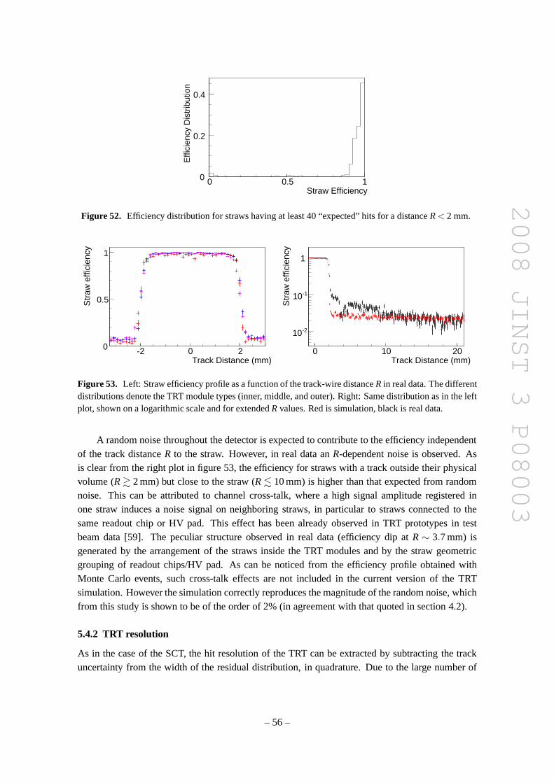
2008 JINST 3 P08003
Straw Efficiency0 0.5 10
0.2
0.4
Effi
cien
cy D
istr
ibut
ion
Figure 52. Efficiency distribution for straws having at least 40 “expected” hits for a distanceR< 2 mm.
Str
aw e
ffici
ency
Track Distance (mm)-2 0 20
0.5
1
Str
aw e
ffici
ency
Track Distance (mm)0 10 20
-210
-110
1
Figure 53. Left: Straw efficiency profile as a function of the track-wiredistanceR in real data. The differentdistributions denote the TRT module types (inner, middle, and outer). Right: Same distribution as in the leftplot, shown on a logarithmic scale and for extendedR values. Red is simulation, black is real data.
A random noise throughout the detector is expected to contribute to the efficiency independentof the track distanceR to the straw. However, in real data anR-dependent noise is observed. Asis clear from the right plot in figure 53, the efficiency for straws with a track outside their physicalvolume (R& 2 mm) but close to the straw (R. 10 mm) is higher than that expected from randomnoise. This can be attributed to channel cross-talk, where ahigh signal amplitude registered inone straw induces a noise signal on neighboring straws, in particular to straws connected to thesame readout chip or HV pad. This effect has been already observed in TRT prototypes in testbeam data [59]. The peculiar structure observed in real data(efficiency dip atR∼ 3.7 mm) isgenerated by the arrangement of the straws inside the TRT modules and by the straw geometricgrouping of readout chips/HV pad. As can be noticed from the efficiency profile obtained withMonte Carlo events, such cross-talk effects are not included in the current version of the TRTsimulation. However the simulation correctly reproduces the magnitude of the random noise, whichfrom this study is shown to be of the order of 2% (in agreement with that quoted in section 4.2).
5.4.2 TRT resolution
As in the case of the SCT, the hit resolution of the TRT can be extracted by subtracting the trackuncertainty from the width of the residual distribution, inquadrature. Due to the large number of
– 56 –
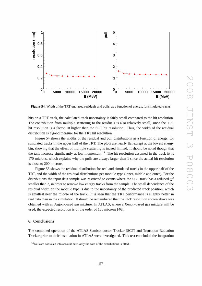
2008 JINST 3 P08003
E (MeV)0 5000 10000 15000 20000
reso
lutio
n (m
m)
0
0.2
0.4
0.6
0.8
1
E (MeV)0 5000 10000 15000 20000
pull
0
1
2
3
4
5
Figure 54. Width of the TRT unbiased residuals and pulls, as a function of energy, for simulated tracks.
hits on a TRT track, the calculated track uncertainty is fairly small compared to the hit resolution.The contribution from multiple scattering to the residualsis also relatively small, since the TRThit resolution is a factor 10 higher than the SCT hit resolution. Thus, the width of the residualdistribution is a good measure for the TRT hit resolution.
Figure 54 shows the widths of the residual and pull distributions as a function of energy, forsimulated tracks in the upper half of the TRT. The plots are nearly flat except at the lowest energybin, showing that the effect of multiple scattering is indeed limited. It should be noted though thatthe tails increase significantly at low momentum.14 The hit resolution assumed in the track fit is170 microns, which explains why the pulls are always larger than 1 since the actual hit resolutionis close to 200 microns.
Figure 55 shows the residual distribution for real and simulated tracks in the upper half of theTRT, and the width of the residual distributions per module type (inner, middle and outer). For thedistributions the input data sample was restricted to events where the SCT track has a reducedχ2
smaller than 2, in order to remove low energy tracks from the sample. The small dependence of theresidual width on the module type is due to the uncertainty ofthe predicted track position, whichis smallest near the middle of the track. It is seen that the TRT performance is slightly better inreal data than in the simulation. It should be remembered that the TRT resolution shown above wasobtained with an Argon-based gas mixture. In ATLAS, where a Xenon-based gas mixture will beused, the expected resolution is of the order of 130 microns [46].
6. Conclusions
The combined operation of the ATLAS Semiconductor Tracker (SCT) and Transition RadiationTracker prior to their installation in ATLAS were investigated. This test concluded the integration
14Tails are not taken into account here, only the core of the distributions is fitted.
– 57 –

2008 JINST 3 P08003
(mm)hit - Rtrackr = R-2 -1 0 1 2
Num
ber
of h
its
0
1000
2000
3000
4000 µ 0.00± 0.00 σ 0.00± 0.20
Data
MC
module layer0 1 2
resi
dual
wid
th (
mm
)
0
0.1
0.2
0.3
0.4
0.5
Data
MC
Figure 55. Comparison of the real and simulated TRT unbiased hit residuals.
process of these two tracking subdetectors and provided thefirst opportunity to test the combinedtracking of SCT and TRT with cosmic rays in a large test stand at the surface integration facility.The four months combined operation of the SCT and TRT allowedthe commissioning and thoroughtesting of the hardware for detector supply, control, and readout systems for the SCT and TRT in afinal detector configuration. The experience of this operation led to numerous improvements in thedetector control, calibration, and physics readout software.
The noise performance of SCT and TRT in the final detector configuration was tested. Thetests showed on the SCT a noise occupancy of 4.7×10⁻⁵ and equivalent noise charge of about1650 electrons for warm operation with hybrid temperaturesapproximately 25◦C above their finalcold operation temperature in the experiment. These results are consistent with previous assemblytest results on single barrels or disks and individual modules during production, showing that thesimultaneous operation of four barrels (nine disks) did notlead to a noise increase. The noise ofthe TRT barrel and endcap was investigated through a series of test runs with the SCT off and withthe SCT operated synchronously with the TRT. The tests showed no increase of noise on the TRTthrough a series of tests with SCT in on and off states. The frontend electronics noise of SCT andTRT during the active readout cycle of the respective other subdetector was tested and the absenceof cross-talk between SCT and TRT in the combined test was confirmed.
During the combined tests of barrel and endcap large samplesof cosmic ray events werecollected. Those events were used to commission the online monitoring software and offline trackreconstruction software chain, which will be used for LHC collisions. The online monitoring wasoperated at the event filter level as well as standalone. Reconstructing the cosmic tracks in SCTand TRT, individually and combined, allowed the successfultesting of raw data processing, trackreconstruction, and detector alignment methods with real data for the first time. This has led to theextraction of first preliminary results for basic tracking performance parameters. A single planeefficiency of 99% and spatial resolution matching expectations from simulation for the SCT were
– 58 –

2008 JINST 3 P08003
found. The TRT drift time resolution of≈200 µm agrees with the expected value for an argon-based gas mixture. Similarly, the measured straw efficiencyis in agreement with expectations.
Acknowledgments
We are greatly indebted to all the technical staff who workedon the integration and testing of theInner Detector from the ATLAS SCT and TRT Institutes. We acknowledge the support of the fund-ing authorities of the collaborating institutes includingthe Spanish National Programme for ParticlePhysics; the Research Council of Norway; the Science and Technology Facilities Council of theUnited Kingdom; the Polish Ministry of Education and Science; the German Ministry of Science;the Swiss National Science Foundation; the State Secretariat for Education and Research and theCanton of Geneva; the Slovenian Research Agency and the Ministry of Higher Education, Scienceand Technology of the Republic of Slovenia; the Ministry of Education, Culture, Sports, Scienceand Technology of Japan; the Japan Society for the Promotionof Science; the Civil Research andDevelopment Foundation and the Office of High Energy Physicsof the United States Departmentof Energy; the United States National Science Foundation; the Australian Research Council (ARC)and Department of Education, Science and Training (DEST); the Dutch Foundation for Fundamen-tal Research on Matter (FOM) and the Netherlands Organisation for Scientific Research (NWO);the Ministry of Education, Youth and Sports of the Czech Republic; the National Science Council,Taiwan; the Swedish Research Council; the European Union (DGXII), the International ScienceFoundation; the Knut and Alice Wallenberg Foundation; the International Science and Technol-ogy Centre; the Natural Science and Engineering Research Council of Canada; the Ministry ofEducation and Science of the Russian Federation; the Academy of Science of the Russian Federa-tion; the International Association for the Promotion of Cooperation with Scientists from the newIndependent States of the former Soviet Union; the Turkish Atomic Energy Authority.
References
[1] ATLAS collaboration,ATLAS: technical proposal for a general-purpose pp experiment at the LargeHadron Collider at CERN, CERN-LHCC-94-43.
[2] ATLAS collaboration,ATLAS Inner Detector Technical Design Report. Volume 1 and 2,CERN-LHCC-97-016, CERN-LHCC-97-017.
[3] A. Abdesselam et al.,The barrel modules of the ATLAS semiconductor tracker, Nucl. Instrum. Meth.A 568 (2006) 642.
[4] A. Abdesselam et al.,The ATLAS semiconductor tracker end-cap module, Nucl. Instrum. Meth.A 575(2007) 353.
[5] A. Ahmad et al.,The Silicon microstrip sensors of the ATLAS semiconductor tracker, Nucl. Instrum.Meth.A 578 (2007) 98.
[6] F. Campabadal et al.,Design and performance of the ABCD3TA ASIC for readout of silicon stripdetectors in the ATLAS semiconductor tracker, Nucl. Instrum. Meth.A 552 (2005) 292.
[7] E. Abat et al.,The ATLAS TRT Barrel Detector, 2008JINST3 P02014.
[8] E. Abat et al.,The End Caps of the ATLAS Transition Radiation Tracker, in preparation.
– 59 –
2008 JINST 3 P08003
[9] E. Abat et al.,The ATLAS TRT Electronic, 2008JINST3 P06007.
[10] S. Terada et al.,Design and development of a work robot to place ATLAS SCT modules onto barrelcylinders, Nucl. Instrum. Meth.A541 (2005) 144.
[11] G. Viehhauser,Macro-assembly of the ATLAS Barrel SCT, IEEE Nucl. Sci. Symp. Conf. Rec.2 (2004)1188.
[12] A. Abdesselam et al.,The Detector Control System of the ATLAS SemiConductor Tracker duringMacro-Assembly and Integration, 2008JINST3 P02007.
[13] CAN in Automation (CiA), http://www.can-cia.de/.
[14] PVSS-II, ETM Austria, http://www.pvss.com/.
[15] http://dim.web.cern.ch/dim/.
[16] P.A. Coe, D.F. Howell and R.B. Nickerson,Frequency scanning interferometry in ATLAS: remote,multiple, simultaneous and precise distance measurementsin a hostile environment, Meas. Sci.Technol.15 (2004) 2175;S.M. Gibson,The ATLAS SCT alignment system and a comparative study of misalignment at CDFand ATLAS, D.Phil. Thesis, Oxford (2004), CERN-THESIS-2007-080.
[17] A. Abdesselam et al.,The Integration and Engineering of the ATLAS SemiconductorTracker Barrel,submitted to JINST.
[18] A. Sfyrla et al.,The Detector Control System for the ATLAS Semiconductor Tracker Assembly Phase,IEEE Trans. Nucl. Sci.52 (2005) 938.
[19] http://itcobe.web.cern.ch/itcobe/Projects/Framework/.
[20] ATLAS Embedded Local Monitor Board,http://www.nikhef.nl/pub/departments/ct/po/html/ELMB128/ELMB22.pdf.
[21] A.J. Barr et al.,The Data Acquisition and Calibration System for the ATLAS Semiconductor Tracker,2008JINST3 P01003.
[22] A. Abdesselam et al.,Engineering for the ATLAS SemiConductor Tracker (SCT) End-cap,2008JINST3 P05002.
[23] ATLAS collaboration,ATLAS high-level trigger, data-acquisition and controls :Technical DesignReport, CERN-LHCC-2003-022.
[24] B.C. LeGeyt and J. Valls,XTRTUsersGuide,http://valls.web.cern.ch/valls/ATLAS_TRT/Files%20TRT/xtrt.htm
[25] T. Vickey,A read-out driver for silicon detectors in ATLAS, Proceedings of 12th Workshop onElectronics for LHC and Future Experiments, LECC2006, Valencia Spain (2006),http://cdsweb.cern.ch/record/1027436.
[26] Amplifier-Shaper-Discriminator-BLR Integrated Circuit, http://www.hep.upenn.edu/atlas/asdblr/.
[27] F. Anghinolfi et al.,DSM-DTMROC: Project Specification,http://www.hep.upenn.edu/atlas/dtmroc/dsm_dtmroc/DSM_DTMROC_Specs_v1_12.pdf.
[28] ATLAS collaboration,ATLAS computing: Technical Design Report, ATLAS-TDR-017,CERN-LHCC-2005-022.
[29] S. Agostinelli et al.,GEANT4 — a simulation toolkit, Nucl. Instrum. Meth.A 506 (2003) 250.
– 60 –

2008 JINST 3 P08003
[30] J. Allison et al.,GEANT4 developments and applications, IEEE Trans. Nucl. Sci.53 (2006) 270.
[31] O.C. Allkofer et al.,The absolute cosmic ray muon spectrum at sea level, Phys. Lett.B 36 (1971) 425.
[32] A. Dar,Atmospheric neutrinos, astrophysical neutrinos and proton decay experiments, Phys. Rev.Lett.51 (1983) 227.
[33] T. Cornelissen,Track fitting in the ATLAS experiment, PhD Thesis, University of Amsterdam (2006),CERN-THESIS-2006-072.
[34] T.H. Kittelmann and E.B. Klinkby,A Study of TRT Noise in 2004 Test Beam Data,ATL-INDET-PUB-2008-010;T.H. Kittelmann,Modelling of Noise and Straw to Straw Variations in the ATLASTransitionRadiation Tracker, ATL-INDET-PUB-2008-009.
[35] F. Åkesson et al.,ATLAS Tracking Event Data Model, ATL-SOFT-PUB-2006-004.
[36] F. Åkesson et al.,ATLAS Inner Detector Event Data Model, ATL-SOFT-PUB-2007-006.
[37] ATLAS Event Display Atlantis, http://www.hep.ucl.ac.uk/atlas/atlantis/.
[38] E.T. Ray,Learning XML, O’Reilly (2003) [ISBN: 0-596-00420-6].
[39] D. Tidwell, XSLT, O’Reilly (2001) [ISBN: 0-596-00053-7].
[40] S. Kolos et al.,Online Monitoring software framework in the ATLAS experiment, Proceeding ofConference for Computing in High-Energy and Nuclear Physics (CHEP2003), La Jolla, CaliforniaU.S.A. (2003), ATL-DAQ-2003-005.
[41] W. Vandelli et al.,Stategies and Tools for ATLAS on-line monitoring, Proceeding of Conference forComputing in High-Energy and Nuclear Physics (CHEP2003), Mumbai, India (2006).
[42] R. Brun and F. Rademaker,ROOT — An Object Oriented Data Analysis Framework, Nucl. Instum.Meth.A 389 (1997) 81, also inProceedings AIHENP’96 Workshop, Lausanne Switzerland (1996);see also http://root.cern.ch/.
[43] F.P. Zema et al.,The GNAM Monitoring system and the OHP histogram presenter for ATLAS, 14th
IEEE-NPS Real Time Conference 2005, Stockholm, Sweden (2005).
[44] Trolltech ASA Sandakerveien 116, Oslo, Norway, http://trolltech.com/.
[45] M. White, Searching for Supersymmetry with the ATLAS Detector, PhD Thesis, University ofCambridge (2006), CERN-THESIS-2008-052.
[46] E. Abat et al.,The ATLAS Transition Radiation Tracker (TRT) proportionaldrift tube: design andperformance, 2008JINST3 P02013.
[47] P.W. Phillips,Functional testing of the ATLAS SCT barrels, Nucl. Instrum. Meth.A 570 (2007) 230.
[48] S.O. Rice,Mathematical Analysis of Random Noise, Bell System Technical Journal23 (1944) 282.
[49] ATLAS SCT collaboration, V.A. Mitsou,Production performance of the ATLAS semiconductortracker readout system, IEEE Trans. Nucl. Sci.53 (2006) 729.
[50] S. Blusk et al.,Proceedings of the first LHC Detector Alignment Workshop, Geneva Switzerland(2006), CERN-2007-004.
[51] F. Heinemann,Robust Track Based Alignment of the ATLAS Silicon Detectorsand Assessing PartonDistribution Uncertainties in Drell-Yann Processes, D.Phil. Thesis, University of Oxford (2007),CERN-THESIS-2007-075.
– 61 –

2008 JINST 3 P08003
[52] P. Bruckman et al.,Global χ2 approach to the Alignment of the ATLAS Silicon Tracking Detectors,ATL-INDET-PUB-2005-002.
[53] A. Bocci and W. Hulsbergen,TRT Alignment For SR1 Cosmics and Beyond,ATL-INDET-PUB-2007-009;T. Golling, , ATL-INDET-PUB-2006-001.
[54] O.K. Øye,Preparing the ATLAS experiment, SemiConductor Tracker commissioning and simulationstudies of SUSY models, Thesis, University of Bergen (2006).
[55] D. Mergelkuhl, A. Wiart,ATLAS - SCT Barrel Detector Photogrammetric Measurement ofSCTBarrel, FSI and Pixel JIG, EDMS document ATL-IS-UR-0004 id 681215 (2005).
[56] E. Dobson, S.M. Gibson, F. Heinemann and M. Karagoz Unel, Study of a twisted ATLAS SCT Barreldeformation as revealed by a photogrammetry survey, ATL-INDET-PUB-2008-011.
[57] F. Campabadal et al.,Beam tests of ATLAS SCT silicon strip detector modules, Nucl. Instrum. Meth.A 538 (2005) 384.
[58] H. Pernegger,Integration and test of the ATLAS semiconductor tracker, Nucl. Instrum. Meth.A 572(2007) 108.
[59] ATLAS TRT collaboration, T. Akesson et al.,ATLAS Transition Radiation Tracker test-beam results,Nucl. Instrum. Meth.A 522 (2004) 50.
– 62 –