Collusive Capacity∗

Daehyun Kim† Rustin Partow‡

November 11, 2019

Abstract

It is widely believed that cartels with too many members are destined to fail. Thestandard argument is that as the number of cartel members increases, shares of collu-sive profit diminish relative to deviation profits. We show that this argument is builton unreasonable assumptions about plant capacity. We add plant capacity choicesto an otherwise standard dynamic oligopoly game. We consider the unsophisticatedand easily enforced strategy in which each firm simply chooses plant capacity equalto static Nash output. Our main result is that as the number of firms goes to infinity,the critical discount factor required to sustain collusion converges to less than 0.63.Thus, collusion is (quite) robust to the number of firms. This result applies to a broadclass of demand functions and to both Cournot and Bertrand competition.

Keywords: Capacity constraints; Collusion; Repeated games.

JEL Classification Numbers: C72, C73, L13, L41.∗We thank Moshe Buchinsky, Maurizio Mazzocco, and Ichiro Obara for their support. For useful discus-

sions and comments, we thank Simon Board, Elhadi Caoui, and Vitaly Titov. All errors are ours.†Department of Mathematical Economics and Finance, Wuhan University. E-mail address:

daehyunkim@whu.edu.cn‡Department of Economics, UCLA. E-mail address: rustinpartow@gmail.com

1

1 Introduction

Economists widely believe that cartels with too many firms are doomed to fail. We arguethat the standard intuition underlying this consensus is flawed because it ignores capac-ity constraints. In this paper, we consider the behavior of a cartel with arbitrarily manymembers, who endogenously choose plant capacity in addition to the usual quantity orprice choices. We show that a relatively unsophisticated and easily enforced strategy con-cerning plant capacity will tend to ensure successful collusion regardless of the numberof members.

In particular, our paper challenges what might be called the splitting-of-the-pie intu-ition, which is well explained in the following excerpt from a European Commission re-port (Ivaldi et al., 2007):

Since firms must share the collusive profit, as the number of firms increaseseach firm gets a lower share of the pie. This has two implications. First, thegain from deviating increases for each firm since, by undercutting the col-lusive price, a firm can steal market shares from all its competitors; that is,having a smaller share each firm would gain more from capturing the entiremarket. Second, for each firm the long-term benefit of maintaining collusion isreduced, precisely because it gets a smaller share of the collusive profit. Thusthe short-run gain from deviation increases, while at the same time the long-run benefit of maintaining collusion is reduced. It is thus more difficult toprevent firms from deviating.

This pie-splitting reasoning is commonly taught in undergraduate economics coursesand appears to be the main reason why cartels with many members are expected to fail.1

This same intuition (applied in reverse) suggests that a possible benefit of antitrust activ-ity is to prevent collusion by reducing concentration. Theory plays an unusually large rolein determining the factors that facilitate collusion because tacit (or sufficiently discrete)cartels are necessarily unobserved. The available evidence from sanctioned or criminallyinvestigated cartels fails to establish a connection between market concentration and col-lusion, as discussed in Levenstein and Suslow (2006).2

The implicit assumption in the above excerpt from Ivaldi et al. (2007) is that capac-ity can be changed spontaneously. In the physical products industries that are typicallymodeled under Cournot competition, output can be easily varied at the margin, but ex-pansions in plant capacity are slow and conspicuous. Any realistic theoretical rendition

1Another possible reason, which we will not challenge in this paper, pertains to the difficulty in moni-toring.

2See table 4 on page 59 for a list of cartels and numbers of participants.

2

Figure 1

of a cartel defection ought not require installing large amounts of new capacity. In thispaper, we claim to show that this is precisely what would needs to happen to force theunraveling of a cartel with many members.

Our basic argument can be easily understood through the mathematics of large cartels.Suppose that a small member of a large cartel deviates from a collusive regime for a one-time increase in output, causing the industry to permanently revert to a price war withzero profit.3 Then letting r denote the interest rate, the cartel member’s percent increasein output must be at least 1

r . For reasonable interest rates, this means a 1,000% increase ormore to make defection attraction.

Can a 1,000% increase in output occur without a conspicuous increase in capacity?The data on excess plant capacity suggest not. In Figure 1, we show the excess capacitiesfor 75 different industries taken from the quarterly Survey of Plant Capacity Utilizationconducted by the US Census Bureau. In the survey, individual plants report their currentquarterly production, and the maximum output that they could feasible have producedin that quarter. Both numbers are aggregated across industries using the NAICS classifi-cation system, and the ratio of the two numbers gives an industry’s capacity utilization.

According to Figure 1, excess capacity seldom averages more than 40% across an in-dustry. Combining our brief mathematical example with the data gives some prima facie

3Here we assume that the firm’s expansion in output by several multiples would have negligible effectson price-cost margins, due to its being small and having constant marginal costs.

3

evidence to suspect that by realistically modeling capacity constriants, the apparent fea-sibility of collusion, and its dependence on the number of cartel members, may change.

In a recent paper, Kuhn (2012) considers a setting where a fixed industry capacity be-comes increasingly fragmented after entry. He finds that collusion may become easierafter the increase, because “Very fragmented markets allow for very severe punishments,while capacity constraints limit the incentives for deviation from a collusive price.” Mean-while, Brock and Scheinkman (1985) consider the case where per-capita capacity is con-stant, and find a non-monotonic relationship between the number of firms and the easeof collusion. In their setting, adding firms initially aids collusion by increasing the sever-ity of punishments, but this effect eventually diminishes and is dominated by the dilutionof collusive profits.

Our main contribution, relative to these papers, is to properly endogenize the choiceof capacity as part of a collusive equilibrium. We present a two-stage game. In stage one,firms simultaneously choose costless and permanent capacity levels. In stage two, theyplay an infinitely repeated oligopoly game, and each firm’s production is constrained bytheir previous capacity choice. We analyze a simple collusive regime in which the firmschoose modest capacity levels and then repeatedly produce equal shares of the monopolyquantity. Defection in both stages is punished with infinite Nash reversion. The importantfeature of the stage-one capacity choice, which is simply the static stage-Nash level ofoutput, is that it remains incentive compatible regardless of any stage one uncertaintyabout whether a cooperative or non-cooperative outcome will be played in stage two.We initially assume that capacity is free, and we later show that relaxing this assumptiondoesn’t qualitatively change the results. We find support for Kuhn’s assumption of fixedindustry capacity. We then derive some practical results on cartel robustness by calcultingasymptotic and uniform bounds on the critical discount factor necessary for collusion.

We proceed with a discount factor analysis that shows that collusive capacity makescollusion on output much easier than is suggested by models that abstract from capacity,and this holds uniformly with respect to the number of firms. As the number of firmsgoes to infinity, industry capacity converges to the constant perfectly competitive out-put level and monopolistic collusion can be achieved with a discount factor above 0.63.For any finite number of firms, we find that a discount factor of 0.732 is sufficient for awide range of demand functions, 2/3 for concave demand functions, and 1/2 for lineardemand functions.

These results suggest that capacity constraints can completely mitigate the number-of-firms effect discussed in Ivaldi et al. (2007). This is because a model with unlimitedcapacity constraints will eventually, as N becomes large, imply deviation payoffs that

4

are unrealistically large when compared to, say, the capacity these firms would need toproduce competitive output levels. It is still possible that collusion becomes harder asthe number of firms increases, but it is probably because of monitoring difficulties andnot because of the incentives effect that is typically emphasized by economists. There area large number of unconcentrated industries with relatively strong monitoring devicessuch as trade associations and industry newsletters.4

Before Kuhn (2012), several other papers also considered capacity investment in anoligopoly model. Davidson and Deneckere (1986) imagine the specific case where twocartel participants merge and insist that there shares of cartel profit be unchanged post-merger. If the cartel relies on a Nash reversion punishment, then the severity of the Nashpunishment will decline, while some of the participants will still get their original shares,increasing their incentives to defect. Benoit and Krishna (1987) study a case similar toours where firms in a duopoly make capacity decisions and compete a-la Bertrand (alsosee Kreps and Scheinkman (1983)). Their focus is to characterize shared properties ofequilibria with above-Nash prices, and they show that excess capacity in every period isa necessity.5

Our paper essentially extends the Benoit and Krishna (1987) setting to incorporate ar-bitrarily many firms. The thrust of their results is that excess capacity plays a role as a“sheathed but visible sword”. Our paper emphasizes that this is its only role. Even if ca-pacity were free, the firms in a minimally sophisticated cartel would carry at most enoughto inflict punishments–anything more than this would threaten to unravel collusion with-out offering any private benefits. To emphasize this we initially assume that capacity iscostless. On the other hand, when capacity is costly, it effectively becomes a public goodand the cartel’s punishment protocol must disincentivize free-riding in the form of capac-ity underinvestment. We discuss costly capacity as an extension towards the end of thepaper.

The rest of this paper is organized as follows. Section 2 describes the basic model. Sec-tion 3 establishes some preliminary results on the robustness of our collusive equilibriumto the number of firms. We then introduce the concept of ρ-concavity (see Anderson andRenault (2003)) and use it to establish stronger results on cartel robustness. Section 4 dis-cusses several extensions, including Bertrand rather than Cournot competition, capacity

4Levenstein and Suslow (2006) find that trade associations are important to the duration of large cartels.5There is also relatively large literature concerning the use of capacity constraints as a pre-commitment

device (e.g., Spence (1977), Fudenberg and Tirole (1984), Bulow et al. (1985), Herk (1993), Spencer andBrander (1992)). In these settings, capacity can be used by an incumbent to deter entry, or by an entranthoping that by setting aside enough residual demand for the incumbent, it will be induced to maintain highprices (the Judo economics technique).

5

adjustment costs, and entry. Section 5 concludes.

2 Dynamic Oligopoly with Irreversible Capacity Investment

Our model is a standard dynamic oligopoly (Cournot) model except that in period t = 0,each firm i ∈ I ≡ {1, 2, . . . , N} simultaneously chooses a capacity xi ∈ R+. An identicalgame is studied by Benoit and Krishna (1987). Capacity investment is costless and per-manent. For each subsequent period t ∈ {1, 2, . . . }, each firm i simultaneously choosesqi ∈ [0, xi).6

Goods are perfectly substitutable and P : R+ → R+ is the industry’s inverse demandfunction. We make the following assumptions on the cost and inverse demand functions:

Assumption 1. Marginal cost is a constant, c ≥ 0.

Assumption 2. P(·) is twice continuously differentiable, with P′(Q) < 0 and P′′(Q)Q +

P′(Q) < 0 for all Q ∈ R+.

Assumption 3. P(Q) < c for some finite quantity Q.

For example, any strictly decreasing, strictly log-concave, and twice continuously dif-ferentiable inverse demand function would satisfy our assumptions. Assumption 2 issimply a regularity condition which is shown in Lemma 2 to be necessary to ensure thatfirm profit functions are strictly concave and submodular, and thus rule out the existenceof multiple equillibria. Assumption 2 is weaker than strict concavity of P. The other twoassumptions are standard assumptions made for tractability.

Each firm’s choice of capacity and following outputs are perfectly publicly observedby the other firms. A firm’s strategy is defined in the usual way: in period t = 0, each firmchooses the capacity; and in each period t ≥ 1, each firm chooses output within its capac-ity level depending on the history, i.e., the capacity choice and past outputs by the all thefirms up to the period. Each firm’s payoff is discounted by a common discounting factorδ ∈ [0, 1). We use subgame perfection as our equilibrium concept, which requires that inevery possible history, the continuation strategy profile constitutes a Nash equilibrium inthe induced subgame.

6Note that firms cannot produce output in period 0, eliminating the need to analyze simultaneousquantity-capacity deviations. The assumption is purely cosmetic, as our equilibrium could easily incorpo-rate a ”feeling-out” stage where firms produce non-collusive output before reaching the collusive capacitylevel.

6

3 Cartel Robustness to the Number of Firms

Our main question is whether collusive profits can be achieved even as the number offirms goes to infinity if firms are allowed to collude in their capacity, and our analysis willspecifically focus on the industry’s ability to achieve monopoly profits.7 In this section, weshow that holding the industry price at the monopoly level (pm) is robust for a large rangeof discount factors. Moreover, it can be achieved with a very simple equilibrium, whichwe will denote as Collusive Capacity.

Note that the definition of Nash reversion in our model accommodates the fact thatfeasible output levels are determined by the capacity decisions in period 0. The Nashequilibrium of the classic Cournot oligopoly game without capacity, which we will simplycall classic Nash output, may not be feasible if some firms have chosen small capacitylevels.8

We will now present results from a special equilibrium of the model where firms buildup capacity levels equal to classic Cournot-Nash output levels, and subsequently producecollusive output. Both components of the equililbrium are supported with the threat ofinfinite Nash reversion following a defection. The ensuing results will show that thissequence of play is an equilibrium for a broad set of possible discount factors, demandfunctions, and numbers of firms, and that as the number of firms goes to infinity, there canbe no other sequence of play that achieves monopoly profit for a lower discount factor.Our results are easily extended to Bertrand competition, although the emphasis is onCournot where capacity constraints are typically more relevant.

Let Qm ∈ R+ be the monopolist industry quantity, let QneN be the static Nash industry

quantity with N firms, let Qpc be the competitive or choke-quantity at which P(Qpc) = c.Given N, let δ(N) denote the critical level of δ for which the grim trigger strategy withNash reversion achieves Qm.

Proposition 1. Under our assumptions,

(a)

δ ≡ limN→∞

δ(N) = 1− Qm

Qpc ≤ 1− 1e≈ 0.632. (1)

In particular, if P(Q) is concave, then 1− Qm

Qpc ≤ 12 .

7This is in line with many papers on collusion, such as Fershtman and Pakes (2000), where firms areassumed only to collude when it is feasible to achieve monopoly profits.

8For example, on any path where all firms have chosen (weakly) less than the equilibrium capacity level,it is a dominant strategy Nash equilibrium of the ensuing repeated game for each firm to set output equalto capacity.

7

(b) Uniform upper bound for δ(N): Let zN ≡πne

Nπm , and suppose it is bounded by some sequence

zN ≤ z. For any N ≥ 2,

δ(N) ≤ 1− NN − 1

1− zN

eN−1

N − zN≤ 1− 1− z

e− z.

(c) Finally, if demand is linear, i.e., P(Q) = a− bQ for some a, b > 0, then δ(N) = 12 for all

N ≥ 2.

Proof. See Appendix.

Proposition 1 illustrates that Nash capacity makes collusion dramatically resilient tothe number of firms. For example, according to our second result, if collusive profits aretwice as high as Nash profits, then a discount factor of 0.775 is sufficient to sustain col-lusion for any number of firms. This corresponds to a maximum interest rate of about29%–much higher than what is typically assumed in the literature. The underlying in-tuition for our results is simple. For large N, deviations are significantly constrained bycollusive capacity, while punishments are unchanged relative to classic grim trigger collu-sive equilibria with infinite capacity. In the classic case, collusive profits go to zero at rateN while deviation profits remain strictly positive. In our equilibrium, deviation profitsalso go to 0 at approximately rate N.9

Our limiting result is quite simple to understand–as N tends to infinity, Nash profitsas a ratio of collusive per-firm profits (which we denote as 1

N Πm) converge to 0, anddeviation profits as a ratio of collusive profits converge to Qpc/Qm. The reason is that, inthe limit, a firm’s capacity becomes arbitrarily small so that, upon deviating, they have anegligible effect on the industry’s price. Hence, the ratio of deviation to collusive payoffsis Qpc/Qm plus a term that is shrinking at rate N. We can write δ(N) = πd/Πm−1

πd/Πm−πneN /Πm ,

and it should now be clear why the right-hand side converges to Qpc/Qm−1Qpc/Qm = 1− Qm

Qpc .Lemma 4 establishes that this limit must be below 1− 1

e = .632 or, under the strongerassumption that inverse demand is concave, below 1

2 .It is particularly convenient that in the most widely studied case of linear demand,

we get an exact result: a discount factor above 12 is necessary and sufficient for collusion,

regardless of the number of firms.

Example 1. Consider the following inverse demand function:

P(Q) = 1−Qα

9This intuition is also owed to Kuhn (2012).

8

3 4 5 6 7 8 9 10N

0.510

0.515

0.520

0.525

0.530

0.535

0.540

∆HNL

(a) When α = 1/2

2 3 4 5 6 7 8 9 10N

0.475

0.480

0.485

0.490

0.495

0.500

∆HNL

(b) When α = 3/2

and let c = 0. We will show that, depending on α, the critical discount factor required forour equilibrium can either increase or decrease with the number of firms. When α > 1,P is strictly concave; while it is strictly convex when α < 1. For any α ≥ 0, it satisfiesAssumption 2.

One can show QneN =

( Nα+N

) 1α and Qm =

(1

α+1

) 1α ; and Qd = N−1

N Qm + 1N Qne. Using

these and from

δ(N) =πd(N)− 1

N Πm

πd(N)− 1N Πne(N)

we obtain different direction of δ as N increases depending on the size of α (see Figure 2aand Figure 2b).

�

Proposition 2. Let δ(N) denote the minimum discount factor for which collusion can be achievedin any symmetric subgame perfect equilibrium, and let δ(N) denote the analagous discount factorfor our equilibrium.

limN→∞

δ(N) = limN→∞

δ(N) (2)

Proof. See Appendix.

Proposition 2 establishes a sense in which our proposed collusive capacity equilib-rium is close-to-optimal. The reason this is not obvious is that in classic repeated Cournotgames, stick-and-carrot strategies of the type considered in Abreu (1986) will generallysupport collusion for a strictly larger set of feasible discount rates than Nash reversionstrategies. This suggests that they may also provide advantages in our setting. In theclassic repeated Cournot oligopoly, a stick-and-carrot strategy’s punishment entails a sin-gle period of very low or even negative profits, followed by a return to collusion. Butto achieve these low initial profits, the stick-and-carrot strategy requires larger capacitythan an infinite reversion strategy. If the industry had enough capacity to impose thisstick-and-carrot punishment, then while the industry’s punishment could be made more

9

severe, deviation payoffs would also increase. We believe there are cases where this trade-off favors Nash reversion, and other cases where it does not.

However, our proposition establishes that for large N, no symmetric SPE can sustaincollusion for a larger set of discount factors. The intuition is simple. As N goes to infinity,the industry capacity converges to Qpc, the perfectly competitive quantity, and the Nashreversion punishment payoff converges to 0, the most severe possible punishment. Sup-pose there exists another sequence of equilibria with a convergent industry quantity, Q,with a strictly smaller limiting critical discount factor. The key to our proof is recognizingthat Q ≤ Qpc. The reason is that if Q > Qpc, the punishment payoff will still converge toa number no less than 0, as with our equilibrium, but the deviation payoff will be strictlylarger than in our equilibrium, causing the limiting critical discount factor to be larger.

Given that Q ≤ Qpc, as N goes to infinity, Nash reversion becomes an arbitrarily close-to-optimal punishment strategy, and producing at full capacity becomes an arbitrarilyclose-to-optimal deviation strategy. This allows for a convenient closed-form analysisof the asymptotic tradeoffs of capacity. The benefit of more capacity is a more severepunishment, and the cost is a larger deviation incentive. Asymptotically, this tradeoffalways favors adding capacity (until capacity equals Qpc).10

The downside of our analysis thus far is that it requires N going to infinity. We wouldlike to establish claims that are independent of N. In the next sub-section, we will intro-duce the concept of ρ-concavity as a means of restricting and analyzing demand in orderto obtain stronger results.

3.1 Demand Curvature and Robustness

We need to place modest restrictions on the curvature of demand in order to extend ourresults to broad classes of demand or numbers of firms. If demand is allowed to be highlyconcave in one region, and highly convex in another, then it is theoretically possible fordeviation payoffs to be very large, and Nash reversion punishments very mild, for anyfinite number of firms. To tackle this issue formally, we use concept of ρ-concavity (con-vexity) that was first applied to the Cournot setting by Anderson and Renault (2003). Ourpreferred interpretation of ρ-concavity (convexity) is that it bounds the rate at which theinverse-elasticity of demand changes in the industry quantity.

10The reason is quite intuitive. For a very large number of firms, each with arbitrarily small capacities, asingle firm’s deviation from collusive output to producing at full capacity has a negligible effect on price.Thus, a one-percent increase in capacity raises deviation profits asymptotically by one-percent. Meanwhile,the elasticity of industry profits with respect to quantity must be strictly less than -1 for any quantity abovethe collusive level. Thus, a one-percent increase in capacity reduces punishment payoffs asymptotically bymore than one-percent.

10

Definition 1. Consider a strictly positive function D with a convex domain B ⊆ R+. Forρ 6= 0, D is ρ-concave if for any p, p′ ∈ B,

(D(λp + (1− λ)p′))ρ ≥ λD(p)ρ + (1− λ)D(p′)ρ, ∀λ ∈ [0, 1].

For ρ = 0, D is 0-concave if

ln D(λp + (1− λ)p′) ≥ λ ln D(p) + (1− λ) ln D(p′), ∀λ ∈ [0, 1].

A strictly positive function D with a convex domain is said to be ρ-convex if the directionof the inequality is opposite.

When ρ = 0, ρ-concave function is log concave. Also note that a linear function is1-concave and 1-convex.

Lemma 1 (Anderson and Renault (2003)11). The following hold:

(a) D is ρ-concave if and only ifψ(Q) ≤ (1− ρ)

where ψ(Q) ≡ −Q P′′(Q)P′(Q)

. Similarly, D is ρ-convex if and only if

(1− ρ) ≤ ψ(Q).

(b) Let D be a strictly positive and decreasing function with a convex domain in R+. Then,there exists a pair of values in the extended real line, ρ′ and ρ′′ such that D is ρ′-concaveand ρ′′-convex. If D is ρ′-concave and ρ′′-convex, then ρ′ ≤ ρ′′.

We call ψ(Q) := −Q P′′(Q)P′(Q)

the curvature of the inverse demand. This is the elasticity ofthe slope of the inverse demand. The lemma says that ρ-concavity (resp. ρ-convexity) ofa demand function provides an upper (resp. lower) bound of the curvature of its inversedemand.

The demand function in Example 1 has the constant curvature of ψ(Q) = 1− α for allQ ∈ [0, 1]. It is therefore both α-concave and α-convex.

Proposition 3 (Asymptotic bound). If D is ρ′-concave and ρ′′-convex, where ρ′′ ≥ ρ′ ≥ −1,then

ξ(ρ′′) ≤ limN→∞

δ(N) ≤ ξ(ρ′)

11This lemma is Proposition 1 and Claim 1 of Anderson and Renault (2003, p.255). For the proof, refer tothe paper.

11

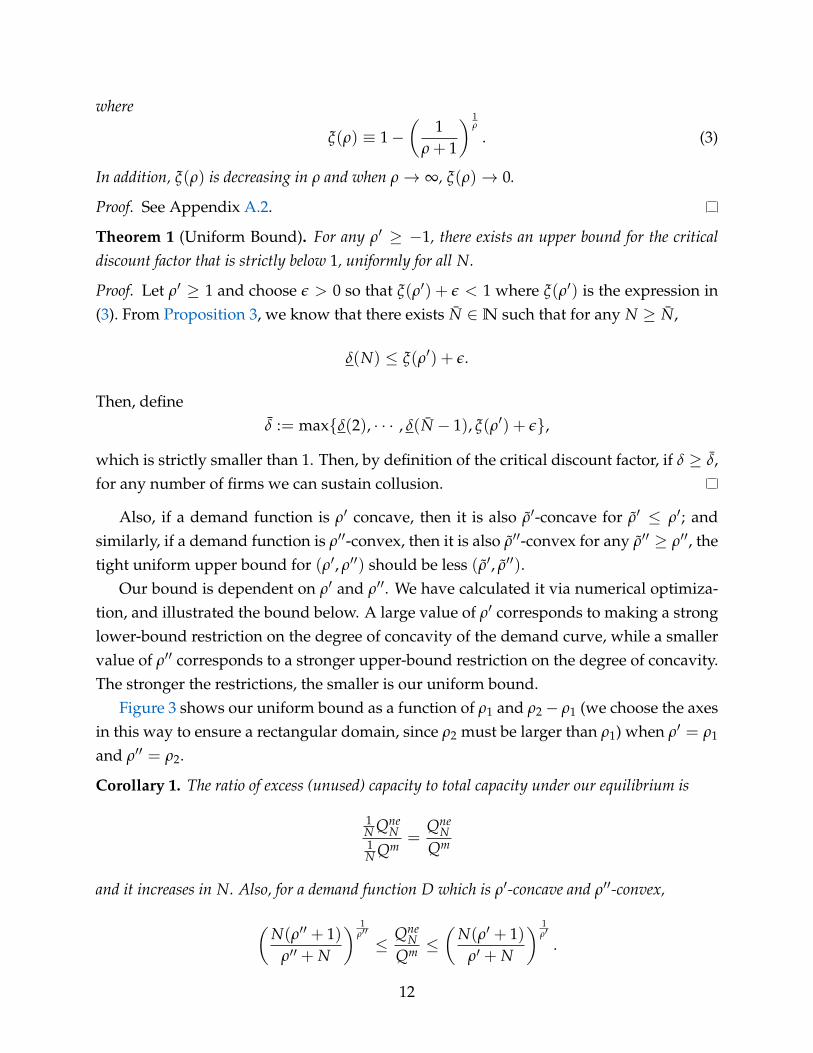
where

ξ(ρ) ≡ 1−(

1ρ + 1

) 1ρ

. (3)

In addition, ξ(ρ) is decreasing in ρ and when ρ→ ∞, ξ(ρ)→ 0.

Proof. See Appendix A.2.

Theorem 1 (Uniform Bound). For any ρ′ ≥ −1, there exists an upper bound for the criticaldiscount factor that is strictly below 1, uniformly for all N.

Proof. Let ρ′ ≥ 1 and choose ε > 0 so that ξ(ρ′) + ε < 1 where ξ(ρ′) is the expression in(3). From Proposition 3, we know that there exists N ∈N such that for any N ≥ N,

δ(N) ≤ ξ(ρ′) + ε.

Then, defineδ := max{δ(2), · · · , δ(N − 1), ξ(ρ′) + ε},

which is strictly smaller than 1. Then, by definition of the critical discount factor, if δ ≥ δ,for any number of firms we can sustain collusion.

Also, if a demand function is ρ′ concave, then it is also ρ′-concave for ρ′ ≤ ρ′; andsimilarly, if a demand function is ρ′′-convex, then it is also ρ′′-convex for any ρ′′ ≥ ρ′′, thetight uniform upper bound for (ρ′, ρ′′) should be less (ρ′, ρ′′).

Our bound is dependent on ρ′ and ρ′′. We have calculated it via numerical optimiza-tion, and illustrated the bound below. A large value of ρ′ corresponds to making a stronglower-bound restriction on the degree of concavity of the demand curve, while a smallervalue of ρ′′ corresponds to a stronger upper-bound restriction on the degree of concavity.The stronger the restrictions, the smaller is our uniform bound.

Figure 3 shows our uniform bound as a function of ρ1 and ρ2− ρ1 (we choose the axesin this way to ensure a rectangular domain, since ρ2 must be larger than ρ1) when ρ′ = ρ1

and ρ′′ = ρ2.

Corollary 1. The ratio of excess (unused) capacity to total capacity under our equilibrium is

1N Qne

N1N Qm

=Qne

NQm

and it increases in N. Also, for a demand function D which is ρ′-concave and ρ′′-convex,

(N(ρ′′ + 1)

ρ′′ + N

) 1ρ′′≤

QneN

Qm ≤(

N(ρ′ + 1)ρ′ + N

) 1ρ′

.

12

Figure 3

Hence, we provide a testable prediction that excess capacity rates should increase withthe number of firms in an industry that is colluding on capacity. Having establishedthese results for the basic Cournot model, the next section will consider several interestingextensions.

4 Extensions

4.1 Capacity Costs

Our job so far has been made relatively easy by the assumption of costless capacity. Whathappens when building capacity requires firms to incur sunk costs? In this section wewill show that when the costs of building capacity are sufficiently small, our results areunchanged. We assume that at t = 0, when firms choose capacity x, they commit topaying periodic costs (1− δ)b(x), for some increasing function b(·). Since these costs aresunk in future periods, adding costs only affects the incentive compatibility of the firstperiod of our strategy profile. Our concepts of monopoly and Nash output will still be

13

based on the one-shot Cournot game without capacity.12

Proposition 4. Suppose that b(·) and N satisfies b(

1N Qne

N

)≤ 1

N (Πm −ΠneN ). Then the Nash

reversion strategy profile remains subgame perfect when there are N firms.

Proof. See Appendix.

Hence, as long as the per-period costs of each firm’s capacity is less than per-periodgains from collusion, the incentive compatibility of our equilibrium will not be affected.There is one desirable property of our equilibrium that we have not preserved in theabove proof. Previously, our collusive capacity level was the same as what firms wouldhave chosen, had they instead anticipated producing Nash output forever. Hence, it re-quired minimal coordination. This is no longer the case in the equilibrium that we use inour proof. It is simple to understand why. Suppose that a firm expects its competitors toeach produce 1

N QneN . It will choose capacity x and then produce x forever. Its anticipated

periodic profits are x(

P(N−1N Qne

N x− c)− b(x). Hence, the new capacity cost term, b(x),

now enters into its stage one decision, and creates an incentive to produce less than Nashoutput. Hence, collusive capacity is no longer identical to non-cooperative capacity.

This property can be easily salvaged, at the cost of exposition, by changing the levelof collusive capacity to equal the new level of non-cooperative capacity. The new level ofnon-cooperative capacity, x?, is the best-response capacity choice in stage one when eachfirm anticipates that the industry will subsequently produce at full capacity forever. Thisis exactly the same as the Nash output level corresponding to the static Cournot gamewhen each firm’s costs of producing q are cq + b(x).This new level of capacity will besmaller than the one we consider above. In general, collusion via a grim trigger pun-ishment, using this capacity level, will require a strictly higher discount factor than thecapacity level that we use in our proof. However, when capacity costs are small, the dif-ferences in these capacity levels, and hence critical discount factors, will be negligible.Thus, we conclude that even with capacity costs, collusion can be sustained with arbitrar-ily many firms, and still requires minimal coordination on capacity.

4.2 Deterring Entry

We have argued that the purpose of excess capacity is to inflict punishments on defectingcartel members. Therefore, a colluding industry should have only enough excess capac-

12In principal, what we are referring to as monopoly output might no longer correspond to the outputdecisions of a forward-looking monopoly, who would consider both capacity costs and variable costs whendetermining its joint capacity and output strategy. However, if capacity costs are small, then so too wouldbe the differences in these levels of output and profits.

14

ity for this purpose, which should correspond to the static Nash output level when thestandard grim trigger punishment is being used. This overlooks another potential usefor excess capacity: deterring potential entrants. From the perspective of the industryincumbents, it may be more profitable to compete and deter entry, than to accomodateentry and subsequently collude. Hence, it is important to check whether the capacityconstraints prescribed in our equilibrium would make an industry more susceptible toentry. Thus, we extend the model to consider endogenous entry.

Suppose that, in addition to the original N firms in the market at stage one, there areinfinitely more firms who can pay an entry cost κ ∈ R+ in order to enter the market at anyperiod during the game, at which point they are in the market permanently. All firms inthe market can make capacity and quantity decisions. However, capacity choices must bemade, and observed, one period before the capacity becomes available to use.13 Assumethat firms compete a-la Cournot and that capacity costs are 0, as in the original model.

It is straightforward to devise a new equilibrium, similar in spirit to our original one,where collusion remains resilient to the number of firms. Let rt ∈ N denote the totalnumber of entrants observed up to period t. Our revised strategy hinges around a criticalnumber of entrants, R ∈ N. If strictly more than R firms choose to enter, the firms willproduce the corresponding level of Nash output. In equilibrium, exactly R firms willenter, all in the first period, and the industry will collude at monopoly output. We willfocus on the equilibrium of this type that delivers the largest profits to the incumbents–theone with the smallest possible number of entrants.

The equilibrium strategy is as follows: In any period where there are fewer than R totalentrants, collude at monopoly output. If there are more than R entrants, or if anyone hasdefected in a previous stage, proceed to the punishment phase. The punishment phaseinvolves producing the stage Nash equilibrium that corresponds to the total number offirms currently in the market, and their respective capacities. Let rt be the number ofentrants in period t. On the equilibrium path, each firm that is in the market choosescapacity equal to 1

N+R QneN+R, and produces output equal to 1

N+R Qm. In the first period, Rfirms enter the market. In all subsequent periods, there is no entry. We call this collusivecapacity with entry deterrence.

Proposition 5. Suppose that in an industry with N ∈ N firms and a given demand function,collusive capacity without entry is an equilibrium for some discount factor δ. Then there existssome R < ∞ for which collusive capacity with entry deterrence is also an equilibrium (for the

13Imagine, for example, the time it takes to build a new manufacturing plant. Notice that this implies thatfirms immediately make capacity decisions after entering, but their competitors observe their new capacitynext period before they are able to start producing.

15

same δ). Moreover, the minimum possible value of R, R, satisfies

R = min{

R ∈N :1

R + N + 1Πne

R+N+1

}≤ κ. (4)

Moreover, R is exactly the same as the number of entrants in the equilibrium where all firmschoose infinite capacity and subsequently produce static Nash output. Hence, we may concludethat collusive capacity does not come at the expense of entry deterrence.

Proof. See appendix.

Our proposition shows that entry will occur up to the point at which entry costs arejust below the Nash profits. This is exactly the same amount of entry that would beexpected in a “competitive” market with unrestricted capacity. Hence, there seems to belittle evidence that the capacity constraints we propose would undermine the industry’sability to deter entry. More importantly, we show that any such entry, if it occured, wouldnot undermine the ability of the cartel to subsequently collude (with the new entrants asmembers).

4.3 Competition in Prices rather than Quantities

In this section, we modify the game so that firms compete choosing prices rather thanquantitities. We assume the efficient rationing rule, which states that aggregate demandis always served first by firms offering the lowest prices, and is then split evenly in thecase of ties.14

Proposition 6. Suppose N ≥ 3 and let δ(N) denote the critical discount factor for which collu-sion can be sustained and let δ denote its limit as N goes to infinity. Then there exists a strategyprofile such that

(a) δ(N) = 1− N−2N

Qm

Qpc ≤ 0.877

(b) δ = 1− Qm

Qpc ≤ 1− 1e .

One such strategy profile is:

• In period 0, each firm i chooses capacity xi =Qpc

N−2 .

• In all periods t ≥ 1, if no firm has deviated, each firm i sets pi = pm.

14Specifying a rationing rule is necessary in settings of price competition with capactiy constraints be-cause, in the event that capacity exceeds demand, payoffs will in general depend on how the scarce demandis allocated to different firms charging potentially different prices.

16

• If there has been exactly one deviation, all firms set price equal to c.

• If there has been more than one deviation, play any stage Nash equilibrium (potentially inmixed strategies).

Proof. See Appendix A.3.

Hence, in a Bertrand setting, our results on capacity constraints are quite similar toour Cournot results.

Unlike the Cournot case, we require industry capacity to be NN−2 times larger than the

Nash output level (in this case, Qpc). If any firm’s capacity is “pivotal” to the industry’sability to produce the Nash punishment quantity, then that firm could profitably deviatefrom the punishment phase by raising price above marginal cost and serving a positiveresidual demand. This implies that at the end of the capacity selection stage, the industrycapacity must exceed N

N−1 Qpc. To ensure that this holds even if one of the firms deviateson capacity selection, each firm must choose 1

N−2 Qpc. These assumptions are similar tothose needed in Kuhn (2012) (see page 1,123).

This equilibrium is no longer robust to miscoordination where firms incorrectly antic-ipate competition at stage one. In such a case, a firm would choose to accumulate 1

N Qpc

instead of the prescribed level. However, this property can be easily recovered with aminor modification at the expense of exposition. Instead of reverting to Nash outputfollowing any deviation, we merely need to introduce some forgiveness with respect todeviations on capacity. Suppose that the industry ignores deviations on capacity when1N Qpc is selected instead of 1

N−2 Qpc. After such a deviation, the industry is still capable ofimplementing the Nash punishment, so the same proof regarding incentive compatibilityapplies.

5 Conclusion

In this paper, we provide theoretical evidence that collusion is more resilient to the num-ber of firms than has been previously thought. In industries where capacity is public andcostly to change, a large number of firms does not necessarily make it difficult to col-lude. On the other hand, if collusion really is harder with more firms, we believe thatmonitoring problems have more theoretical appeal than the incentive problems typicallyemphasized in the literature.

We see the most fruitful avenue for extending our work to be one that incorporatescollusive capacity into an empirical framework such as that in Fershtman and Pakes

17

(2000). Their paper considers the consequences of collusion on technological investment,entry and exit, and welfare in a differentiated product Bertrand setting. Collusion in theirmodel is dictates that, conditional on the industry state, firms produce monopoly outputwhenever doing so is supported by a grim-trigger punishment and otherwise play a stageNash equilibrium. But a potential shortcoming of their paper is that investment decisionsare made unilaterally. They do not consider how a (tacit) cartel would potentially ben-efit from collusive investment, also supported by grim-trigger punishment. Our paperprovides some theoretical evidence that collusive investment strategies can qualitativelyincrease the scope for collusion while remaining very tractable.

A Appendix

A.1 Omitted Proofs

A.1.1 Useful Lemmas

Let π(Qi, qi) denote the profits of firm i given the sum of its competitors quantities, Qi ∈R+, and its own quantity, qi ∈ R+.

Lemma 2. Under our Assumptions 1,2 and 3,

1. The profit-maximizing choice of qi is submodular in Qi

2. π(Qi, qi) is a strictly concave and twice continuously differentiable function

3. For all Q, q ≥ 0P′′(Q + q)q + P′(Q) < 0.

Proof. The FOC of firm i’s profit with respect to its own output is

π2(Q−i, qi) = P′(Q−i + qi)qi + P(Q−i + qi)− c = 0 (5)

By differentiating the equation with respect to Q−i yields

π21 + π22dqi

dQ−i= 0. (6)

Submodularity requires that dqidQ−i

< 0, and concavity requires that π22(Q−i, qi) < 0.Hence, (6) implies π21(Q−i, qi) < 0. Derivation of (5) with respect to Qi yields

π21 = P′′(Q−i + qi)qi + P′(Q−i + qi).

18

Since above we showed that π21 < 0 , the first result follows. The second result followsimmediately from the assumption that demand is decreasing in Q.

The remaining lemmas make the assumption that

P′′(Q + q)q + P′(Q) < 0, ∀Q, q ≥ 0

and P′(Q) < 0, ∀x ≥ 0.

Lemma 3. The Nash first-order condition (5) implies

P(QneN )− c +

1N

QneN P′(Qne

N ) = 0, ∀N ∈N. (7)

By totally differentiating (18) w.r.t. N,

P′(QneN )

dQneN

dN− 1

N2 QneN P′(Qne

N ) +1N

dQneN

dNP′(Qne

N ) +1N

QneN P′′(Qne

N )dQne

NdN

= 0

ordQne

NdN

=Qne

N P′(QneN )

N(

NP′(QneN ) + (P′(Qne

N ) + QneN P′′(Qne

N ))

Because we assume that P′ < 0 and P′′(x)x+ P′(x) < 0, the above equation implies the followinginequality:

0 <dQne

NdN

<1

N2 QneN . (8)

Lemma 4. 1. The industry Nash output QneN is increasing in N

2. For all K, N ∈N, K < N

1 <Qne

NQne

K< e

N−KNK < e,

andlim

N→∞P(Qne

N ) = c

thuslim

N→∞πne

N → 0.

Moreover, if P(Q) is concave, then

1 <Qne

NQne

K≤ N

N + 1K + 1

K, ∀K, N ∈N, K < N.

19

Proof. The Nash first-order condition (5) implies

P(QneN )− c +

1N

QneN P′(Qne

N ) = 0, ∀N ∈N. (9)

By totally differentiating (18) w.r.t. N,

P′(QneN )

dQneN

dN− 1

N2 QneN P′(Qne

N ) +1N

dQneN

dNP′(Qne

N ) +1N

QneN P′′(Qne

N )dQne

NdN

= 0

ordQne

NdN

=Qne

N P′(QneN )

N(

NP′(QneN ) + (P′(Qne

N ) + QneN P′′(Qne

N ))

Because we assume that P′ < 0 and P′′(x)x + P′(x) < 0, the above equation implies thefollowing inequality:

0 <dQne

NdN

<1

N2 QneN . (10)

We can express the Nash quantity with the following integral, for K < N:

QneN = exp

(ln Qne

K +∫ N

K

d ln QneM

dMdN)

(11)

= exp(

ln QneK +

∫ N

K

d ln QneM

dMdM)

(12)

< exp(

ln QneK +

∫ N

K

1M2 dM

)(13)

where the last inequality comes from (10) and solving this integral yields

1 <Qne

NQne

K< e

N−KNK < e, ∀K, N ∈N, K < N.

Next, we will prove the limit result. Since QneN is increasing in N, as shown above,

and is bounded above by Q (see Assumption 3), it must converge. Taking the limit of theNash FOC in (18) as N goes to infinity, and noting that P′(Qne

N ) must be bounded becauseP(Q) was assumed to be twice continuously differentiable, we have

limN→∞

P(QneN ) = c

Finally, we will derive the tighter bound on the growth of the Nash quantity with

20

respect to N under the assumption that P is concave. From (10), we have

dQneN

dN=

QneN

N(

P′′(QneN )

P′(QneN )

QneN + (N + 1)

)≤

QneN

N(N + 1)

where the second inequality comes from P′′(Q) ≤ 0. Thus,

d ln QneN

dN≤ 1

N(N + 1).

Applying this to (11) and solving the integral yields

1 <Qne

NQne

K≤ N

N + 1K + 1

K.

Lemma 5. When firms have classic Nash output as capacity, an optimal one-shot deviation froma collusive output level is to produce at capacity.

Proof. When other firms produce N−1N Qne

N (equal shares of the industry Nash quantity),the optimal response is to produce 1

N QneN (this is the definition of a symmetric Nash

equilibrium). Under collusion, firms produce strictly less than equal shares of Nash out-put, so the unconstrained best response is to produce strictly more than 1

N QneN . (2) also

showed that our assumptions guarantee that profits are concave in a firm’s own quan-tity, which implies that when the unconstrained best response would involve produc-ing above capacity, the constrained best response must be to produce at capacity, whichequals 1

N QneN .

Lemma 6. Suppose Q > Qm. Then P(Q)− c ≤ (Pm − c) QQm .

Proof. The elasticity of price-cost margins with respect to quantity must be larger in ab-solute value than 1 for all quantities above the monopoly quantity (otherwise we do nothave a unique monopoly quantity, and we require demand functions that pose uniqueNash equilibria for all numbers of players N = 1, ..., ∞).

Hence,ln(P(Q)− c) ≤ ln(Pm − c)− (ln Q− ln Qm)

Thus,

ln(P(Q)− c) ≤ (Pm − c)Qm

Q

21

A.1.2 Proof of Proposition 1

Proof. By Lemma 2,P′′(Q + q)q + P′(Q) < 0, ∀Q, q ≥ 0

and P′(Q) < 0, ∀x ≥ 0. Under collusion with Nash capacity, the minimal value of δ, δ, forwhich this is an equilibrium satisfies

δ(N) =πd

N −1N Πc

πdN −

1N Πne

N=

NπdN −Πc

NπdN −Πne

N

where πd(N) denotes an optimal deviation when N− 1 other players are producing equalshares of collusive output, Πc denotes industry collusive profits, and Πne denotes indus-try Nash profits. The collusive output level is assumed to remain fixed as N varies. Hence,Qm must be uniformly smaller than Qne

N for all N. In other words, the maximal possiblevalue of Qm for this exercise is Qpc (we will show that Qne

N increases in N and convergesto Qpc) and the minimal possible value is Qm.

First, we will derive the limiting value of δ(N), as N goes to infinity.

limN→∞

δ(N) =limN→∞ Nπd

N −Πc

limN→∞ NπdN − limN→∞ Πne

N.

By Lemma 5, an optimal deviation is to produce 1N Qne

N . Hence,

limN→∞

Nπd(N) = limN→∞

NQne

NN

(P(

N − 1N

Qc +1N

QneN

)− c)

. (14)

By Lemma 4,

limN→∞

Nπd(N) =

(lim

N→∞Qne

N

)(P(Qc)− c)

= Qpc (P(Qc)− c) .

Also, industry Nash profits converge to 0,15

limN→∞

NπneN = lim

N→∞Qne

N (p(QneN )− c) = Qpc(p(Qpc)− c) = 0

15Note the importance here of constant marginal cost.

22

Finally, note that NΠm = Qm (P(Qm)− c). Substituting in these results, we have

limN→∞

δ(N) =Qpc (P(Qc)− c)−Qm (P(Qm)− c)

Qpc (P(Qc)− c)= 1− Qm

Qpc ≤ 1− 1e

where the last inequality comes from Lemma 4.Second, we will prove the uniform bound result.

δ(N) =πd

N/πm − 1πd

N/πm − πneN /πm

. (15)

The numerator is smaller than the denominator. Hence, applying the quotient rule re-veals that the expression must be increasing in πd

N/πm. The expression is also obviouslyincreasing in πne

N /πm. Thus, to obtain an upper-bound for δ(N), it is sufficient to replaceπd

N/πm and πneN /πm with upper-bounds.

Let πd = QneN(

P(Qd)− c), and write Qd = λQne

N + (1− λ)Qm, where λ = 1N . Then

πd = Qd(

P(Qd)− c)+(

QneN −Qd

) (P(Qd)− c

)= π(Qd) +

(Qne

N −Qd) (

P(Qd)− c)

.

Because π(Q), the industry profit under homogenous output, is strictly concave, weknow that π(Qd) = π

(λQne

N + (1− λ)Qm) > λπ(QneN ) + (1− λ)πm. Hence,

πd < λπneN + (1− λ)πm +

(Qne

N −Qd) (

P(Qd)− c)

= λπneN + (1− λ)πm + (Qne

N − (λQneN + (1− λ)Qm))

(P(Qd)− c

)= λπne

N + (1− λ)πm + (1− λ) (QneN −Qm)

(P(Qd)− c

)< λπne

N + (1− λ)πm + (1− λ) (QneN −Qm) (Pm − c)

From Lemma 4, we know that QneN < e

N−1N Qm. Hence,

πd < λπneN + (1− λ)πm + (1− λ)

(e

N−1N − 1

)Qm (Pm − c)

= λπneN + (1− λ)πm + (1− λ)

(e

N−1N − 1

)πm,

23

which upon dividing by πm implies

πd

πm < λπne

Nπm + (1− λ) + (1− λ)

(e

N−1N − 1

)= λ

πneN

πm + (1− λ)(

eN−1

N

).

Plugging this into (15) and letting z ≡ πneN

πm , we have

δ(N) =

πdN

πm − 1πd

Nπm − πne

Nπm

<λ

πneN

πm + (1− λ)(

eN−1

N

)− 1

λπne

Nπm + (1− λ)

(e

N−1N

)− πne

Nπm

=λ

1−λ z + eN−1

N − 11−λ

eN−1

N − z

= 1− 11− λ

1− z

eN−1

N − z.

Replacing λ = 1N and rearranging terms, we have

δ(N) ≤ 1− NN − 1

1− z

eN−1

N − z≤ 1− 1− z

e− z. (16)

A.1.3 Proof of Proposition 2

Proof. For each N ∈ N, let Q(N) denote an industry capacity under which δ(N) can beachieved. Because the equilibrium is assumed to be symmetric, each firm’s capacity isQ(N)/N.

Claim 1. For any sequence of equilibria whose limiting critical discount rate is less than 1, thereexists a finite N ∈N such that for N ≥ N,

Q(N)

N= arg max

qi∈[0, Q(N)

N

] qi

(P(

qi +N − 1

NQm)− c)

.

In addition, Q(N) is uniformly bounded over N.

In words, when there are sufficiently large number of firms the optimal deviationinvolves producing at capacity.

24

Proof. Such an N must exist because without binding capacity constraints, the criticaldiscount rate must go to 1, whereas we proved in Proposition 1 that with binding capacityconstraints, a critical discount rate less than 1 is achievable.

Also,1N

Q(N)→ 0.

Note that

δ(N) ≥Q(N)(P( 1

N Q(N) + N−1N Qm)− c)−Qm(P(Qm)− c)

Q(N)(P( 1N Q(N) + N−1

N Qm)− c)− 0

If Q(N) is not uniformly bounded the RHS is arbitrarily close to 1.

Assume that Q(N) converges to Q < ∞.16 We henceforth assume that N ≥ N whereN satisfies Claim 1.

We will now show that Q ≤ Qpc. Suppose instead that Q > Qpc. Note that thelimiting punishment payoff (times N) is Πp ≥ 0. The limiting deviation payoff (times N)is Q (P(Qm)− c).17 However, by reducing capacity to Qpc and playing a Nash reversionstrategy, we can always achieve a limiting punishment payoff of 0, but a strictly lowerlimiting deviation payoff (times N) of Qpc (P(Qm)− c). Thus, Q ≤ Qpc.

Having established that Q ≤ Qpc, and therefore Q(N) ≤ Qpc + κ(N) for some se-quence κ(N) → 0 and κ(N) > 0, we will explain why the punishment payoff for anyalternative sequence of collusive equilibria achieves payoffs that are no larger than whatwould be achieved if the industry produced at capacity forever (“capacity reversion”,for short). This will justify analyzing the alternative equilibria as if they used a simplecapacity reversion punishment.

Recall that

δ(N) =πd

N − πm

πdN − π

pN

=Πd

N −Πm

ΠdN −Πp

N

where ΠpN is the lowest strongly symmetric equilibrium payoff.

16This is without loss in generality. To achieve δ(N), capacity must eventually become bounded. Thus,Q(N) is bounded and by Bolzano-Weirstrass, has a convergent subsequence. Hence, if Q(N) did not con-verge, we could always consider instead a convergent subsequence. The limiting discount factor of thatsubsequence must also lie below the limiting discount factor of our equilibrium, otherwise the suppositionthat the original sequence achieved a critical discount rate below δ(N) is wrong. Thus, it is sufficient toprove that no convergent subsequence is asymptotically better than our equilibrium sequence.

17As long as industry capacity is bounded (by assumption), in the limit, an individual firm’s deviationhas no effect on price.

25

Claim 2. For each N ∈N,

ΠpN ≡ Nπ

pN ≥ Q(N)(P(Q(N))− c).

Namely, the industry profit from the worst punishment industry is greater than thatfrom “capacity reversion.”

Proof. In any symmetric equilibrium, where each firm produces the same output, in anyperiod involving punishment a firm’s profit is 1

N Q(P(Q)− c) for some Q ≥ 0.First we claim that in any punishment involving the industry output greater than Qm,

the harshest punishment is achieved when the industry output is Q(N). This is simplybecause for Q > Qm, the industry profit Q(P(Q)− c) is decreasing.

Given this, it is sufficient for the result to show that any punishment that involves theindustry output less Qm in one or more periods cannot be the harshest punishment. Thisis because, deviation from these punishment periods would be strictly more profitable thandeviation from collusive output itself. Formally, consider firm i’s deviation and supposeQ−i <

N−1N Qm, then,

maxqi∈[0, 1

N Q(N)]qi(P(qi + Q−i)− c) ≥ 1

NQm

(P(

1N

Qm + Q−i

)− c)

>1N

QmP((Qm)− c).

We should emphasize that “capacity reversion” may not actually be subgame perfect(it is certainly not when Q(N) > Qne

N ). Our purpose is merely to provide a lower boundfor the worst possible punishment payoff that could be subgame perfect.

From the above discussion, we can proceed to consider alternative sequences of equi-libria achieving critical discount rate sequence δ(N) which (1) have asymptotic industrycapacity Q ∈ [Qm, Qpc] , (2) use capacity reversion as punishment, and (3) where an opti-mal deviation is to produce at capacity.

By Claim 1, the deviation payoff satisfies

Πd = limN→∞

NπdN = Q (P(Qm)− c) .

And by Claim 2, the punishment payoff, πpN, satisfies

Πp = limN→∞

NπpN ≥ Q (P(Q)− c) .

26

Thus,

δ ≡ limN→∞

δ(N) =Q(P(Qm)− c)−Qm(P(Qm)− c)

Q(P(Qm)− c)−Πp

≥ δ(Q) ≡ Q(P(Qm)− c)−Qm(P(Qm)− c)Q(P(Qm)− c)− Q(P(Q)− c)

. (17)

Because the critical discount rate is increasing in the punishment payoff, a lower bound isformed by replacing the punishment payoff with its upper bound that was given above.

Since the Nash reversion equilibrium we construct yields the critical discounting fac-tor of δ(Qpc), it is sufficient for the conclusion to show that δ(Q) is indeed decreasingover [Qm, Qpc]. Although the direction of δ(Q) is a priori not obvious (note that there is atrade-off of having a larger capacity; i.e., harsher punishment and larger deviation gain),the following claim shows that this is the case.

Claim 3. δ(Q) in (17) is decreasing over [Qm, Qpc].

Proof. Let P(Q) ≡ P(Q)− c. Then,

δ′(x) =P(Qm)(xP(Qm)− xP(x))− (P(Qm)− P(x)− xP′(x))(xP(Qm)−QmP(Qm))

(xP(Qm)− xP(x))2.

Let

η(x) ≡ P(Qm)(xP(Qm)− xP(x))− (P(Qm)− P(x)− xP′(x))(xP(Qm)−QmP(Qm))

Note that at Qm, η(x) is 0; so is δ′(x). Thus, to show δ′′(x) ≤ 0 for all x ≥ Qm, it issufficient that η(x) is decreasing.

dη(x)dx

= P(Qm)(P(Qm)− P(x)− xP′(x))

− (−P′(x)− xP′′(x))(xP(Qm)−QmP(Qm))− (P(Qm)− P(x)− xP′(x))P(Qm)

= −(−P′(x)− xP′′(x))(xP(Qm)−QmP(Qm))

≤ 0

where the last inequality comes from Assumption 2.

Thus, the derivative is non-positive over the entire interval [Qm, Qpc], and we canconclude that δ(Q) < δ(Qpc). Hence, no other sequence of equilibria can admit a broaderset of discount factors than ours, asymptotically.

27

A.1.4 Proof of Proposition 5

Proof. We want to solve for the minimum value of R that makes this an equilibrium. If the(R + 1)th firm enters the market, then its competitors will revert to the non-cooperativeoutcome: producing N + R + 1-firm Nash output, 1

N+R+1 QneN+R+1. Anticipating this, a

best response is for these entrants is to respond by choosing capacities and subsequentoutputs of 1

N+R+1 QneN+R+1, obtaining profits of 1

N+R+1 πneN+R+1 − κ. The ex-ante profits

of this non-cooperative outcome, from the perspective of an entrant, is decreasing in R,holding N fixed. Thus, the minimum value of R is the smallest number for which thenon-cooperative outcome with R + 1 entrants is not profitable. I.e., we need to find

min{

R ∈N :1

R + N + 1Πne

R+N+1

}≤ κ.

Because Nash profits converge to 0 with N (Lemma 4), as long as κ is strictly positive,there must be some R < ∞ for which this holds. In periods 2 and after, one can simplymodify all of our previous results on N firms to account for R + N + 1 firms. We can usethe same uniform bound for δ that was previously obtained in Proposition 1. Note thatthe resulting bound is even smaller than that using the original number of firms, N.18

Finally, we will prove the last statement regarding the number of firms that wouldenter when all firms are choosing infinite capacity and subsequently competing by pro-ducing static Nash output. The proof is trivial. First, assume that firm capacity andoutput strategies do not depend on the actions of other firms. Then clearly, conditionalon the number of entrants in the first period, it is subgame perfect for each individualfirm to choose infinite capacity and to produce the static Nash output level (by defini-tion of Nash equilibrium) in each period. In each period, it must be unprofitable foran additional firm to enter the market. Consider the last period of entry, T (readersmay anticipate that actually, all entry must occur in period 1, but this is not necessaryfor the proof). The entering firm will pay period cost κ forever, and earn period prof-its of 1

R+N+1 πnR+N+1 forever. Hence, the smallest possible number of entrants satisfies

R = min{R : 1RT+N+1 πn

RT+N+1}.

A.1.5 Proof of Proposition 4

Proof. First, note that setting deviant capacity, x, larger than the prescribed Nash capacityis clearly never profitable since it involves greater spending on capacity and worse profitsin the subsequent supergame. Assume that deviations at future stages are unprofitable

18This does not necessarily mean that entry actually makes collusion easier, because we haven’t identifiedthe exact critical discount factor for arbitrary demand functions.

28

so that we can focus on how the introduction of costs affects the robustness of our results.A deviation to a capacity of x < 1

N QneN produces the following per-period profit forever:

π(x) ≡ −b(x) + x(

P(

N − 1N

QneN + x

)− c)

.

If the firm conforms to the equilibrium capacity, it gets

−b(

1N

QneN

)+

1N

QmP(Qm).

The gains to deviation are (in per-period terms)

π(x)−(

1N

Πm − b(

1N

QneN

))= b

(1N

QneN

)− b(x) + x

(P(

N − 1N

QneN + x

)− c)− 1

NΠm

≤ b(

1N

QneN

)+

1N

ΠneN −

1N

Πm

where the last inequality comes from the definition of Nash equilibrium, i.e., the termx(

P(

N−1N Qne

N + x)− c)

is maximized at x = 1N Qne

N , achieving the value of 1N Πne

N . Asufficient condition for deviations to be unprofitable is, therefore,

b(

1N

QneN

)≤ 1

N(Πm −Πne

N ).

A.2 Proof of Proposition 3

The proof follows from the sequence of lemmas given below.

Lemma 7. For any N ∈N,

d ln Π(QneN )

dN= −(N − 1)

d ln QneN

dN.

Proof.ln Π(Qne

N ) = ln QneN + ln(P(Qne

N )− c)

andd ln Π(Qne

N )

dN=

dQneN

dN

[1

QneN

+1

P(QneN )− c

P′(QneN )

]

29

From the FOCs for the Nash equilibrium, we have

P(QneN )− c +

1N

QneN P′(Qne

N ) = 0

⇐⇒ 1 +1N

QneN

P′(QneN )

P(QneN )− c

= 0

P′(QneN )

P(QneN )− c

= − NQne

N

Thus,

d ln Π(QneN )

dN=

1Qne

N

dQneN

dN(1− N)

= −(N − 1)d ln Qne

NdN

.

Lemma 8. For any N ∈N,

d ln QneN

dN=

1N(ψ(Qne

N ) + N + 1) .

Proof. The Nash first-order conditions for each firm imply

P(QneN )− c +

1N

QneN P′(Qne

N ) = 0, ∀N ∈N. (18)

By totally differentiating (18) with respect to N, we get

P′(QneN )

dQneN

dN− 1

N2 QneN P′(Qne

N ) +1N

dQneN

dNP′(Qne

N ) +1N

QneN P′′(Qne

N )dQne

NdN

= 0

ordQne

NdN

=Qne

N P′(QneN )

N(

NP′(QneN ) + (P′(Qne

N ) + QneN P′′(Qne

N )) .

Dividing both sides by QneN P′(Qne

N ) and applying the definition ψ(QneN ) = Qne

NP′′(Qne

N )P′(Qne

N )

yieldsd ln Qne

NdN

=1

N(

N + 1 + ψ(QneN )) .

30

Lemma 9. For any N ∈N,

d ln Π(QneN )

dN= −N − 1

N1

ψ(QneN ) + N + 1

.

Proof. This comes from straightforward application of Lemma 7 and Lemma 8.

Lemma 10. Suppose demand is ρ′-concave. Then

Π(Q)

Π(Qm)≤ Q

Qm

(1− 1

ρ′

((

QQm )ρ′ − 1

)).

Proof. Observe that

−P′(Q) = −P′(Qm) exp∫ ln Q

ln Qm

d ln(−P′(Q))

d ln Qd ln Q.

Using Lemma 1, we have

d ln(−P′(Q))

d ln Q=−P′′(Q)Q−P′(Q)

= −ψ(Q) ≥ ρ′ − 1,

and we also know from the monopoly FOC that

P′(Qm) = −Pm − cQm .

Applying the two properties yields

−P′(Q) ≥ Pm − cQm exp

(∫ ln Q

ln Qm

(ρ′ − 1

)d ln Q

),

=Pm − c

Qm

(Q

Qm

)ρ′−1

.

This implies

P(Q) = P(Qm) +∫ Q

QmP′(q)dq ≤ P(Qm)−

∫ Q

Qm

(Pm − c

Qm

(q

Qm

)ρ′−1)

dq

= Pm − Pm − c(Qm)ρ′

(Qρ′

ρ′− (Qm)ρ′

ρ′

)

31

From this,

=⇒ P(Q)− c ≤ Pm − c− (Pm − c)1ρ′

(Qρ′ − (Qm)ρ′

)=⇒ P(Q)− c

Pm − c≤ 1− 1

ρ′

((

QQm )ρ′ − 1

)=⇒ Q (P(Q)− c)

Qm (Pm − c)≤ Q

Qm

(1− 1

ρ′

((

QQm )ρ′ − 1

))=⇒ Π(Q)

Π(Qm)≤ Q

Qm

(1− 1

ρ′

((

QQm )ρ′ − 1

)).

Lemma 11. Suppose that D, market demand, is ρ′-concave and ρ′′-convex, with ρ′′ ≥ ρ′. Thenfor any N > K, (

N(ρ′′ + K)K(ρ′′ + N)

) 1ρ′′≤

QneN

QneK≤(

N(ρ′ + K)K(ρ′ + N)

) 1ρ′

,

and (ρ′ + Kρ′ + N

)(1+ 1ρ′) (

NK

) 1ρ′≤

Π(QneN )

Π(QneK )≤(

ρ′′ + Kρ′′ + N

)(1+ 1ρ′′) (

NK

) 1ρ′′

.

Proof. From Lemma 9, we have

d ln Π(QneN )

dN= −N − 1

N1

ψ(QneN ) + N + 1

.

From Lemma 1, we have

1ρ′′ + N

≤ 1ψ(Qne

N ) + N + 1≤ 1

ρ′ + N.

Thus,

−N − 1N

1ρ′ + N

≤d ln Π(Qne

N )

dN≤ −N − 1

N1

ρ′′ + N.

In turn, this implies

−∫ N

K

M− 1M

1ρ′ + M

dM ≤ lnΠ(Qne

N )

Π(QneK )≤ −

∫ N

K

M− 1M

1ρ′′ + M

dM

32

Note that

−∫ N

K

(1− 1

M

)1

ρ + MdM = −

∫ N

K

(1

ρ + M− 1

ρ

(1M− 1

ρ + M

))dM

= −∫ N

K

1ρ + M

((1 +

1ρ

)− 1

ρ

1M

)dM

= −[(

1 +1ρ

)ln(ρ + M)

∣∣∣∣NK− 1

ρln M

∣∣∣∣NK

]

= − ln

(ρ + Nρ + K

)(1+ 1ρ

) (KN

) 1ρ

= ln

( ρ + Kρ + N

)(1+ 1ρ

) (NK

) 1ρ

Thus, (

ρ′ + Kρ′ + N

)(1+ 1ρ′) (

NK

) 1ρ′≤

Π(QneN )

Π(QneK )≤(

ρ′′ + Kρ′′ + N

)(1+ 1ρ′′) (

NK

) 1ρ′′

.

From Lemma 8, and using D is ρ′-concave,

1Qne

N

dQneN

dN=

1N(ψ(Qne

N ) + (N + 1))

≤ 1N((ρ− 1) + N + 1)

=1

N(ρ′ + N).

Thus,

QneN ≤ exp

(ln Qne

K +∫ N

K

1M(ρ′ + M)

dM)

= exp(

ln QneK +

∫ N

K

1ρ

(1M− 1

ρ′ + M

)dM)

when ρ 6= 0. Thus,Qne

NQne

K≤ e

1ρ ln

(N(ρ+K)K(ρ+N)

)

In a similar way, since D is ρ′′-convex, we can obtain

1N(ρ′′ + N)

≤ 1Qne

N

dQneN

dN

33

and thus we have (N(ρ′′ + K)K(ρ′′ + N)

) 1ρ′′≤

QneN

QneK≤(

N(ρ′ + K)K(ρ′ + N)

) 1ρ′

In particular, when K = 1,

(N(ρ′′ + 1)

ρ′′ + N

) 1ρ′′≤

QneN

Qm ≤(

N(ρ′ + 1)ρ′ + N

) 1ρ′

Thus,

1−(

ρ′′ + NN(ρ′′ + 1)

) 1ρ′′≤ 1− Qm

QneN≤ 1−

(ρ′ + N

N(ρ′ + 1)

) 1ρ′

, ∀N ∈N.

Taking N to infinity for each term, we obtain

1−(

1ρ′′ + 1

) 1ρ′′≤ 1− Qm

Qpc ≤ 1−(

1ρ′ + 1

) 1ρ′

,

where we remind the reader that Qpc is the perfectly competitive quantity–the limitingvalue of Nash output. When ρ′ → 0, the upper bound goes to 1− 1

e . When ρ′ = ρ′′ = 1(i.e., when D is concave), both the lower and upper bounds converge to 1

2 .

A.3 Proof of Proposition 6

Proof. We only need to check whether there is a profitable one-shot deviation on the equi-librium paths, and the off-the-equilibrium paths in which only one firm has ever deviated(because for the other off-the equilibrium paths, firms play a static Nash equilibrium).

Unilaterally deviating at the capacity stage generates 0 profits forever and is unprof-itable compared to the collusive outcome.

Consider a deviation from an off-the equilibrium path in which there has been onlyone deviation. First, consider the case in which there was a unilateral deviation in ca-pacity choice. Consider a deviation by a firm i to set a lower price than pm. Since theother firms set price 0, and the sum of their capacity is at least Qpc (this is because, in thecapacity choice, even in the case the deviated firm k (assume k 6= i) chose 0 capacity,

∑j 6=i

xj ≥ 0 + ∑j 6=i,k

xj = (N − 2)Qpc

N − 2= Qpc

where xj is firm j’s capacity. If k = i, then the sum is even bigger as (N − 1) Qpc

N−2 . Inwords, their is no residual demand for firm i, so setting price c is incentive compatible. An

34

immediate implication is that in such off-the-equilibrium paths, the continuation payoffis 0.19

Now consider a one-shot unilateral deviation from a history on the equilibrium path att ≥ 1. The profits under deviation are maximized by slightly undercutting pm and sellingat maximum capacity. In the previous paragraph, we have shown that the continuationpayoff following this deviation is 0. Thus, the deviation is unprofitable if and only if

1N

Qm pm ≥ (1− δ)1

N − 2Qpc pm

Thus, the critical discount rate is given by

δ = 1− N − 2N

Qm

Qpc .

Finally, we can use ρ-concavity and ρ-convexity to bound the right-hand-side.

Lemma 12.

QneK

(NK

K + ρ′′

N + ρ′′

) 1ρ′′≤ Qne

N ≤ QneK

(NK

K + ρ′

N + ρ′

) 1ρ′

,

and

QneK

(K + ρ′′

K

) 1ρ′′≤ Qpc ≤ Qne

K

(K + ρ′

K

) 1ρ′

.

Proof. Suppose that demand is ρ′-concave and ρ′′-convex, Lemma 8 states that d ln QneN

dN =1

N(N+1+ψ(QneN ))

. By Lemma 1, we therefore know that 1N(N+ρ′′) ≤

d ln QneN

dN ≤ 1N(N+ρ′) .

For N > K, we have

QneN = Qne

K exp(∫ N

K

d ln QneM

dMdM)

. (19)

We will use the aforementioned bounds to bound QneN in terms of Qne

K .

∫ N

K

1M (M + ρ′′)

dM ≤∫ N

K

d ln QneM

dMdM ≤

∫ N

K

1M (M + ρ′′)

dM,

which, by integrating, implies

ln M− ln(M + ρ′′)|NKρ′′

≤∫ N

K

d ln QneM

dMdM ≤

ln M− ln(M + ρ′)|NKρ′

,

19For this argument, we need N ≥ 3. We do not know whether we can dispense this assumption.

35

or equivalently,

1ρ′′

ln(

NK

K + ρ′′

N + ρ′′

)≤∫ N

K

d ln QneM

dMdM ≤ 1

ρ′ln(

NK

K + ρ′

N + ρ′

).

Applying this to Equation 19 yields

QneK exp

(1

ρ′′ln(

NK

K + ρ′′

N + ρ′′

))≤ Qne

N ≤ QneK exp

(1ρ′

ln(

NK

K + ρ′

N + ρ′

)),

which simplifies to

QneK

(NK

K + ρ′′

N + ρ′′

) 1ρ′′≤ Qne

N ≤ QneK

(NK

K + ρ′

N + ρ′

) 1ρ′

,

Finally, taking the limit as N goes to infinity, and writing Qpc = limN→∞ QneN , we have

QneK

(K + ρ′′

K

) 1ρ′′≤ Qpc ≤ Qne

K

(K + ρ′

K

) 1ρ′

.

Using Lemma 12, with K = 1, we conclude that (1 + ρ′′)1

ρ′′ ≤ Qpc

Qm ≤ (1 + ρ′)1ρ′ .

Applying this to our earlier expression for the critical discount rate yields

1− N − 2N

(1 + ρ′

) 1ρ′ ≤ δN ≤ 1− N − 2

N(1 + ρ′′

) 1ρ′′ .

Thus, taking the limit as N → ∞, we get bounds for the asymptotic critical discountrate, δ:

1−(

11 + ρ′

) 1ρ′≤ δ ≤ 1−

(1

1 + ρ′′

) 1ρ′′

.

Finally, a set of uniform bounds can be derived by letting N go to infinity on the left-hand-side, and letting N = 3 in the right-hand-side.

0 ≤ δ ≤ 1− 13

(1

1 + ρ′′

) 1ρ′′

.

36

References

Abreu, Dilip (1986), “Extremal equilibria of oligopolistic supergames.” Journal of EconomicTheory, 39, 191–225.

Anderson, Simon P. and Regis Renault (2003), “Efficiency and surplus bounds in cournotcompetition.” Journal of Economic Theory, 113, 253–264.

Benoit, Jean-Pierre and Vijay Krishna (1987), “Dynamic duopoly: Prices and quantities.”The review of economic studies, 54, 23–35.

Brock, William A and Jose A Scheinkman (1985), “Price setting supergames with capacityconstraints.” The Review of Economic Studies, 52, 371–382.

Bulow, Jeremy, John Geanakoplos, and Paul Klemperer (1985), “Holding idle capacity todeter entry.” The Economic Journal, 95, 178–182.

Davidson, Carl and Raymond Deneckere (1986), “Long-run competition in capacity,short-run competition in price, and the cournot model.” The Rand Journal of Economics,404–415.

Fershtman, Chaim and Ariel Pakes (2000), “A dynamic oligopoly with collusion and pricewars.” The RAND Journal of Economics, 207–236.

Fudenberg, Drew and Jean Tirole (1984), “The fat-cat effect, the puppy-dog ploy, and thelean and hungry look.” The American Economic Review, 74, 361–366.

Herk, Leonard F (1993), “Consumer choice and cournot behavior in capacity-constrainedduopoly competition.” The RAND Journal of Economics, 399–417.

Ivaldi, Marc, Bruno Jullien, Patrick Rey, Paul Seabright, and Jean Tirole (2007),The Political Economy of Antitrust (Contributions to Economic Analysis, Volume282), chapter The Economics of Tacit Collusion:Implications for Merger Con-trol, 217–239. URL https://www.emeraldinsight.com/doi/abs/10.1016/

S0573-8555%2806%2982008-0.

Kreps, David M and Jose A Scheinkman (1983), “Quantity precommitment and bertrandcompetition yield cournot outcomes.” The Bell Journal of Economics, 326–337.

Kuhn, Kai-Uwe (2012), “How market fragmentation can facilitate collusion.” Journal of theEuropean Economic Association, 10, 1116–1140.

37

Levenstein, Margaret C and Valerie Y Suslow (2006), “What determines cartel success?”Journal of economic literature, 44, 43–95.

Spence, A Michael (1977), “Entry, capacity, investment and oligopolistic pricing.” The BellJournal of Economics, 534–544.

Spencer, Barbara J and James A Brander (1992), “Pre-commitment and flexibility: Appli-cations to oligopoly theory.” European Economic Review, 36, 1601–1626.

38