collocation methods general approach for ordinary...

Palestine Journal of Mathematics

Vol. 7(2)(2018) , 650–662 © Palestine Polytechnic University-PPU 2018

COLLOCATION METHODS GENERAL APPROACH FORORDINARY DIFFERENTIAL EQUATIONS

K.P.Mredula1,2 and D. C. Vakaskar2

Communicated by I. Lasiecka

MSC 2010 Classifications: Primary 65Y20, 42C40; Secondary 65G30, 65T60.

Keywords and phrases: Boundary value problem, initial value problem, solution of ordinary differential equation,generalized wavelet collocation procedure.

Abstract The article discusses generalized method for solving ordinary differential equationusing wavelet collocation method. The method is implemented for both the initial valued problemsas well as boundary valued problems. We can directly solve the boundary valued problem asagainst the traditional shooting methods where the boundary valued problem itself is approximatedby Initial valued problem and hence we achieve better accuracy with wavelet collocation methods.

1 Introduction

The theory of wavelets is being utilized for the past two decades in various applications ofsignal processing, fingerprint verification [7], storing fingerprint electronically using wavelet,denoising data , musical tones, etc see [8] and solution of differential equations [5],[3], [4].Wavelets have several properties which are encouraging their use for numerical solutions ofdifferential equations. The orthogonal, compactly supported wavelet basis exactly approximatespolynomial of increasingly higher order. This wavelet basis can provide an accurate and stablerepresentation of differential operations even in region of strong gradients or oscillations. Inaddition, the orthogonal wavelet basis has the inherent advantage of multi resolution analysisover the traditional methods [4]. The adaptive wavelet collocation method is able to dynamicallytrack the evolution of the solution’s irregular features and to allocate higher grid density to thenecessary regions. Therefore, the number of collocation points needed is optimized, withoutdamaging the accuracy of the solution [5]. The benefit of Haar wavelet approach is their sparsematrices representation, fast transformation and possibility of implementation of fast algorithms[8].In this article we brief the collocation method used for solving initial valued problem andboundary valued problem with simple examples to establish a common unified approach ofapproximating derivative using wavelet function as basis.In this method higher order derivative is approximated using wavelet function and the lower orderderivatives and functions itself are expressed by repeated integration. The orthogonal set of Haarfunctions is used. This group of square waves has magnitude ±1 in some interval and zeroelsewhere. These zeros make Haar transform faster than other square functions such as Walshsfunctions. Haar wavelet basis lacks differentiability and hence the integration approach will beused instead of the differentiability for calculation of coefficients. Due to the local property ofthe powerful Haar wavelet the new method is simpler.This article has been organized in the following way. Section 2 discusses the prerequisitesfor understanding Haar wavelets as a basis function and their properties. Section 3 describeshow a function can be represented using Haar wavelets as basis function. Section 4 discussesinitial value problem formation using haar wavelets. Section 5 describes solution for boundaryvalue problem with four different types of boundary conditions. Section 6 explains a commonprocedure to handle examples of both initial value and boundary value problem. Section 9explains normalization procedure for a general solution of IVP and BVP within domain [A,B].Section [11] and 8 discusses examples of IVP and BVP respectively. Section 10 describestransformation of a boundary valued problem using the general transformation discussed insection 9. Section 11 explains along with an example of IVP, how to extend the solution to

WAVELET BASED SOLUTIONS 651

a specified value with increased resolution , since the basis is valid within [0, 1]. The examplesare validated using plots utilizing Matlab code.

2 Basis wavelet

Haar wavelets are considered as basis wavelets in the discussion, haar transform has been usedas an earliest example for orthonormal wavelet transform with compact support. Haar wavelettransform has been used as an earliest example for orthonormal wavelet transform with compactsupport. The Haar wavelet transform is the first known wavelet and was proposed in 1909 byAlfred Haar. The Haar wavelet family for,x ∈ [0, 1) Is defined by,

hi(x) =

1 if x ∈ α, β)−1 if x ∈ [β, γ)

0 elsewhere.(2.1)

here,

α =k

mβ =

k + 0.5m

γ =k + 1m

(2.2)

here m = 2j , j = 0, 1, , J. indicates the levels of wavelet and integer k = 0, 1, .., (m − 1),the shift parameter. Maximum resolution is J , and i = m + k + 1. Incase of minimum valuem = 1, k = 0, i = 2 The maximal value of i is i = 2M = 2J + 1 The function

h1(x) =

{1 x ∈ [0, 1)0 elsewhere.

(2.3)

From equation (2)

h2(x) =

1 if x ∈ 0, 0.5)−1 if x ∈ [0.5, 1)0 elsewhere.

(2.4)

which can be graphically vizualized as,

Figure 1. Haar function

The equation 2.3 is also called mother wavelet. In order to perform wavelet transform, Haarwavelet uses translations and dilations of the function, i.e. the transformation uses the followingfunction

h(x) = h(2j − k) (2.5)

Translation/Shifting with h(x) = h(x− k)Dilation/Scaling with h(x) = h(2jx) where this is the basic work for wavelet expansion. With

652 K.P.Mredula1,2 and D. C. Vakaskar2

the dilation and translation process as in Eq.(2.5), one can easily obtain father wavelet, daughterwavelet, granddaughter wavelet etc.

Figure 2. Haar wavelets representation upto second resolution

We can obtain coefficient matrix H of order 2m× 2m as

H =

1 1 1 11 1 − 1 − 11− 1 0 00 0 1 − 1

for m = 2, The Haar wavelets are orthogonal as, i.e. The operational matrix P which is a 2msquare matrix is define as in [12] by

pi,1(x) =

x∫0

hi(x′)dx′ (2.6)

Figure 3. Integratral representation of Haar wavelets

and the recurrence relation is given by

pi,v+1(x) =

x∫0

pi,v(x′)dx′ where v = 1, 2, ... (2.7)


We will need the integral

P (x) =

x∫A

x∫A

...

x∫A

hi(t)dtu =

1(u− 1)!

x∫A

(x− t)u−1hi(t)dt (2.8)

with u = 2, 3, ..., n and i = 1, 2, ..., 2m The above integrals can be evaluated using equation 2the first two are given by

pi,1(x) =

x− α for x ∈ [α, β)

γ − x for x ∈ [β, γ)

0 elsewhere.(2.9)

pi,2(x) =

12(x− α)

2, for x ∈ [α, β)1

4m2 − 12(γ − x)

2, for x ∈ [β, γ)1

4m2 , for x ∈ [γ, 1)0 elsewhere.

(2.10)

and so on will be utilized in representing the derivative and function values in the furtherdiscussion.

3 Function representation

Considering the fact that Haar functions are orthogonal, we may take any function f(x) whichis square integrable in the interval [0, 1) as an infinite sum of Haar wavelets,

f(x) =∞∑i=1

aihi(x) (3.1)

where ai are haar coefficients and hi(x) are haar wavelet functions. f(x) has finite terms and iff(x) is piecewise constant or can be approximated as piecewise constant during each subintervalas,

f(x) =2M∑i=1

aihi(x) (3.2)

In this scheme the highest order derivative of the function is approximated by haar wavelets andthe consecutive lower order derivatives and function itself is obtained by repeated integration asexplained in the section IV and V.

4 Initial Value Problem IVP

Consider the general nth order linear differential equation

M1yn(x) +M2y

(n−1)(x) + ...+Mny(x) = f (4.1)

for x ∈ [A,B] with initial condition

y(n−1)(A), y(n−2)(A), ..., y(A) (4.2)

and all lower order derivative approximations are obtained by repeated integrals. For examplerth order derivative of y is obtained as

yr(x) =2M∑i=1

aipi,n−r(x) +n−r−1∑σ=0

1σ!

(x−A)σy(r+σ)0 (4.3)


We obtain y(n−1)(x), y(n−2)(x), ... and y(x) The collocation points are obtained by

xp =(p− 1

2)

2M, p = 1, 2, ... 2M (4.4)

The expressions of yn(x), y(n−1)(x), and y(x) are substituted in differential equation, discretizationis applied along the points given by equation (4.4) resulting in a linear or non linear system of2M × 2M . Solving the system for haar coefficients the approximate solution is achieved.

5 Boundary value problems BVP

Consider a second order boundary valued problem

y”(x) = f(x, y, y′) (5.1)

for x ∈ [0, 1] For second order ordinary differential equations, there are four different types ofboundary conditions possible. They are treated differently as follows

Case 1 y(0) = R and y(1) = Q then integrating equation (5.1) yields

y′(x) =2M∑i=1

aipi,1(x) + y′(0) as pi,1(0) = 0.

Integrating again and using condition y(0) = R we get

y(x) = R+ y′(0)x+2M∑i=1

aipi,2(x). (5.2)

Now utilizing second condition y(1) = Q we obtain y′(0) = (Q − R) −2M∑i=1

aici1 with

ci1 =∫ 1

0 pi,1(x)dx further simplifying we get

y(x) = R+ (Q−R)x+2M∑i=1

ai(pi,2(x)− xci1) (5.3)

and

y′(x) = Q−R+2M∑i=1

ai(pi,1(x)− ci1) (5.4)

Case 2 y′(0) = R1 and y(1) = Q1 Integrating equation (5.1) and using boundary condition,y′(0) = R1 we get

y′(x) = R1 +2M∑i=1

aipi,1(x) (5.5)

y(x) = Q1 −R1(1− x)−2M∑i=1

ai(ci1 − pi,2(x)) (5.6)

Case 3 y(0) = R2 and y′(1) = Q2 we get

y′(x) = Q2 − a1 +2M∑i=1

aipi,1(x) (5.7)

and

y(x) = R2 + (Q2 − a1)x+2M∑i=1

ai(pi,2(x)) (5.8)


Case 4 y′(0) = R3 and y′(1) = Q3 here by integrating and applying the first condition we obtain,

y′(x) = R3 +2M∑i=1

aipi,1(x) using y′(1)

(Q3 −R3) = a1 as pi,1(1) = 1.(5.9)

so we get

y”(x) = (Q3 −R3)h1(x) +2M∑i=2

aihi(x) (5.10)

y′(x) = R3 + (Q3 −R3)p11(x) +2M∑i=2

aipi1(x) (5.11)

(5.12)

y(x) = y(0) +R3x+ (Q3 −R3)p12(x) +2M∑i=2

aipi2(x) (5.13)

which is obtained by equation (5.9), by integrating from 0 to x. Similarly we can extend theapproach to higher order differential equations with boundary conditions.

6 Procedure• The highest order derivative is approximated by haar wavelet function.

• The successive lower order derivatives and the function itself is replaced by the expressionsobtained by repeated integration obtained in (i)

• The algebraic expression in terms of haar coefficients is represented in matrix form.

• The matrix is solved to obtain the haar coefficients ai which are then substituted in theexpression of solution function.

Separate MATLAB routines are generated for computation of the matrix P and C which appearin the algebraic representation. P represents the matrix formed by Pi,k and C represents thematrix formed by required C ′i,ks , where k depends on the order of the equation handled. Nowto get a clear idea of the methods we give examples, one each for second order initial valuedproblem and second order boundary value problem in the next sections.

7 Example 1

Consider an initial valued ordinary differential equation,

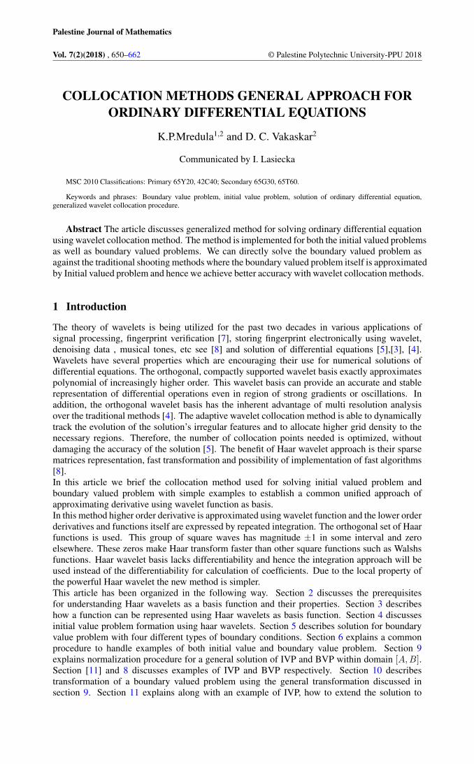
y” + y = sin(x) + x cos(x) (7.1)

with x ∈ [0, 1] and y(0) = 1 and y′(0) = 1 The analytic solution is given by

y(x) = cosx+54

sinx+14(x2 sinx− x cosx) (7.2)

Wavelet formulation is obtained by substituting y”(x) =∑2Mi=1 aihi(x) and integrating twice this

equation we get

y(x) =2M∑i=1

aipi2(x) + 1 + x (7.3)


The differential equation gets converted to

2M∑i=1

ai(hi(x) + pi,2(x)) = sinx+ x cosx− 1− x (7.4)

Solving the system A[H + P ] = B we obtain the wavelet coefficient matrix A, where H is thehaar matrix, P is the matrix consisting with rows P ′i,ks and B is right hand side vector obtainedby considering values of x at collocation points. From the expression y(x) of by substituting thewavelet coefficients, the solution function is generated. For j=3, that is m=16. We obtained theresult, compared it with analytical solution using MATLAB program. The plot is given in fig(4).

Figure 4. Comparison of haar solution with exact solution for example 1 using j = 3

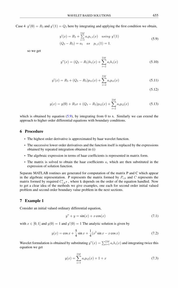
Now fig (5) represents the graph of the haar, analytical and inbuilt function implementationof matlab results for the initial valued problem (Example 1).

Figure 5. Plot for Haar implementation, analytic and inbuilt solution


8 Example 2

Consider a second order boundary valued problem as y” = y′+y+expx(1−2x) with x ∈ [0, 1]with condition y(0) = 1 and y(1) = 3e which are the boundary conditions as mentioned in case1. The analytical solution of this boundary valued problem is y = expx(1 + 2x) Taking thewavelet approximation for second derivative, we obtain

y′(x) = 3e− 1 +2M∑i=1

ai(pi,1(x)− ci1) and

y(x) = 1 + (3e− 1)x+2M∑i=1

ai(pi,2(x)− xci1)(8.1)

Therefore the boundary valued problem gets transformed as

2M∑i=1

ai(hi(x)− pi,1(x) + ci1(1 + x)− pi,2(x)) = x(3e− 1)

+ex(1− 2x) + 3e.(8.2)

For 2m collocation points we get 2m linear algebraic equations with unknowns 2m haar coefficients,which are obtained by solving the system of equations. By substituting the coefficients ai soobtained in the equation for y(x) we get the required solution. This result is compared with theanalytical solution which is exactly similar at j = 3, that is m = 16, as in fig (9)

Figure 6. Comparison of haar solution with exact solution for example 2

The graph of the haar, analytical and inbuilt function implementation of matlab results forthe boundary valued problem (Example 2) using , j = 3, is below.


Figure 7. Comparison of haar solution with exact solution for BVP

8.1 Observations

We have presented a unified way for solving the initial valued problem and the boundary valuedproblem using the wavelet collocation method. As we stated earlier this method is bound togive more accurate solution for boundary valued problem compared to the traditional shootingmethods. Also an appropriate higher wavelet resolution may be chosen if the ordinary differentialequation is stiff. To improve the accuracy and optimize the computation an appropriate dynamicresolution adaptive scheme could be formulated. In case of nonlinear differential equation withrelatively less non linearity, it generates manageable non linear algebraic equations; otherwise itbecomes a complicated system. Our method is more amicable for linear differential equations.

9 Normalization procedure for general solution of ivp and bvp within thedomain [0, 1].

Since Haar wavelet function is defined in [0, 1] the collocation method with haar basis functioncan be used for obtaining solution in interval [0,1], when we seek solution either for initialvalue or boundary value ordinary differential equation in domain [A,B], we need to carryouttransformation as follows Consider a boundary valued ordinary differential equation as (5.1) x ∈[A,B] with conditions specified at any random points A and B as y(A) and y(B) we transformthe variable x to x1 such that x1 lies in the interval [0, 1] with the transformation, x1 = x−A

B−Awhich leads to a change in the differential equation and boundary conditions. Derivatives willchange with this transformation.

dy

dx=

dy

dx1(dx1

dx), (9.1)

d2y

dx2 =d

dx(dy

dx) =

d

dx1(dy

dx)dx1

dx

Accordingly the boundary conditions are modified and obtained between [0, 1], once the aboveformulation is done, the equation can be solved as specified in an example. Finally the solutionis again transformed back to the original variable with specified parametric changes to obtainthe results in the domain [A,B]. Another possibility is extending the solution for an arbitraryinterval [A,B] with initial conditions specified at 0 , we convert the interval first to an interval[B −A, 0] and solving it for [0, B −A] which is further transformed into [0, 1] as required. Thisconversion helps in converting the problem to the required domain [0, 1] where haar collocationin implemented. Reverse conversion to [A,B] gives the required solution. Here the variable


x1 = B − x which simply converts say for n = 1

dy

dx=

d

dx1(dx1

dx) (9.2)

(9.3)

for n = 2

d2y

dx2 =d

dx(dy

dx) =

d

dx1(−dydx1

) (9.4)

dx1

dx=

d2y

dx12

(9.5)

The above concept is used in example as discussed in this section.

10 Example 3

Consider a simple second order boundary valued problem as

y” = 1, (10.1)

x ∈ [−2, 2] (10.2)

y(−2) = y(2) = 4. (10.3)

Here a change in variable as mentioned in the above section is done with x1 =x+2

4 the modifiedequation obtained using the change of variable both for the differential operator and the boundaryconditions is y”(x)

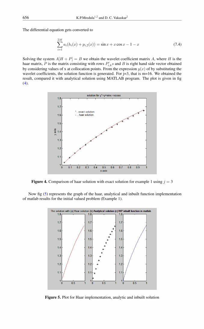
16 = 1 with y(0) = y(1) = 4 The analytical solution of this boundary valuedproblem is y = 8x2 − 8x+ 4 the wavelet formulation is obtain as,

y”(x) =2M∑1=1

aihi(x) (10.4)

y′(x) =2M∑i=1

ai(pi,1(x)− ci1)

y(x) = 4 +2M∑i=1

ai(pi,2(x)− xci1)

Therefore the boundary valued problem gets transformed as∑2M

1=1 aihi(x) = 16 For 2m collocationpoints we get 2m linear algebraic equations with unknowns 2m haar coefficients, which areobtained by solving the system of equations. By substituting the coefficients ai so obtained inthe equation for y(x) we get the required solution. This result is compared with the analyticalsolution which is exactly similar at j = 4, that is m = 32, as in figure 8.


Figure 8. Comparitive study of normalized approche

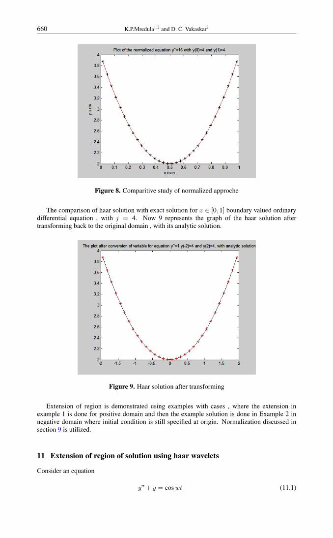
The comparison of haar solution with exact solution for x ∈ [0, 1] boundary valued ordinarydifferential equation , with j = 4. Now 9 represents the graph of the haar solution aftertransforming back to the original domain , with its analytic solution.

Figure 9. Haar solution after transforming

Extension of region is demonstrated using examples with cases , where the extension inexample 1 is done for positive domain and then the example solution is done in Example 2 innegative domain where initial condition is still specified at origin. Normalization discussed insection 9 is utilized.

11 Extension of region of solution using haar wavelets

Consider an equation

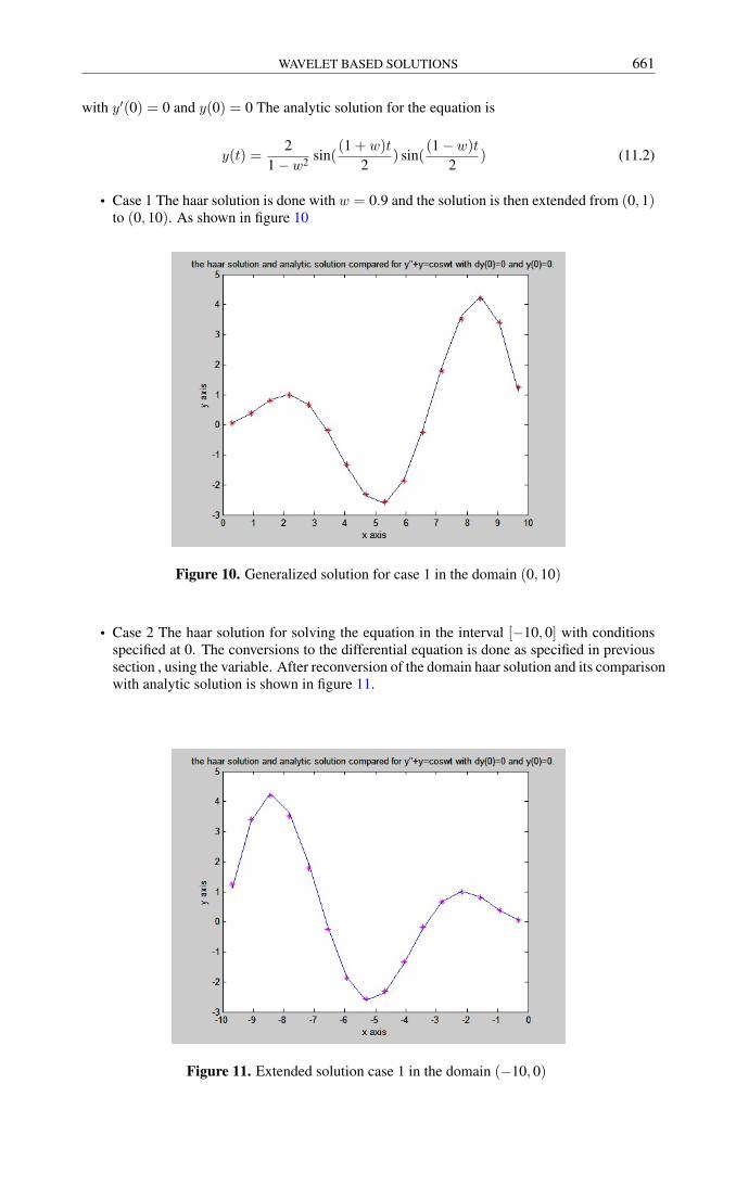
y” + y = coswt (11.1)


with y′(0) = 0 and y(0) = 0 The analytic solution for the equation is

y(t) =2

1− w2 sin((1 + w)t

2) sin(

(1− w)t2

) (11.2)

• Case 1 The haar solution is done with w = 0.9 and the solution is then extended from (0, 1)to (0, 10). As shown in figure 10

Figure 10. Generalized solution for case 1 in the domain (0, 10)

• Case 2 The haar solution for solving the equation in the interval [−10, 0] with conditionsspecified at 0. The conversions to the differential equation is done as specified in previoussection , using the variable. After reconversion of the domain haar solution and its comparisonwith analytic solution is shown in figure 11.

Figure 11. Extended solution case 1 in the domain (−10, 0)


12 Conclusion

The article presents a unified procedure for solving ordinary differential equation using waveletcollocation method for both initial value and boundary value problems. These are discussedwith examples specifying the details of formulation and validation is done using programsdeveloped by us. Results are shown with plots. It demonstrates methodology for solvingordinary differential equation using wavelets in any given domain even though the basis functionis defined in [0, 1]. Hence generalizing is done using the collocation approach with change invariables. Graphical details are interpreted using plots depicting higher resolution in fig 11. It isan efficient and more accurate numerical method for solving ordinary differential equation as wesolve the system of algebraic equation with less calculation rather than solving the differentialequations. The results obtained shows good agreement with analytical solutions.

References[1] Adefemi sunmonu., Implementation of wavelet Solutions to Second order differential equations with

Maple .,Applied Mathematics and Science, Vol 6, 2012.

[2] C.F.Chen, C.H.Hsiao. ,Haar wavelet method for solving lumped and distributed parameter systems., IEEProce.- Control Theory and Appl., vol 144,N0.1, 1997.

[3] Haydar Akca, Mohammed H. Al-Lail, Vallery Covachev.,Survey on Wavelet Transform and Applicationin ODE and Wavelet Networks Advances in Dynamical Systems and Applications., ISSN 0973-5321Volume 1 Number 2 (2006), pp. 129âAS162.

[4] M.A.H. Dempster, A. Eswaran., Solution of PDE by Wavelet Methods. Research Papers in ManagementStudies. WP/2001.

[5] Paulo Cruz AdeHlio Mendes F.D. Magalhaes., Using wavelets for solving PDEs an adaptive collocationmethod, Chemical Engineering Science, 56 (2001)

[6] Mani Mehra., Wavelet and Differential Equations-a short review., 01.30.Cc. http://web.iitd.ac.in/ mmehra,May 2009.

[7] M. Sifuzzaman M.R. Islam and M.Z. Ali., Application of Wavelet Transform and its AdvantagesCompared to Fourier Transform., Journal of Physical Sciences, Vol. 13, 2009, 121-134.

[8] Manoj Kumar Sapna Pandit., Wavelet Transform and Wavelet Based Numerical Methods an IntroductionInternational Journal of Nonlinear Sciences,(2012).

[9] R.J.E. Merry, Wavelet Theory and Applications., A literature study. Eindhoven, June 7, 2005.

[10] SirajâARulâARIslam, B. Sarler, I. Aziz and F. Haq, Haar wavelet collocation method for the numericalsolution of boundary layer fluid flow problems, International Journal of Thermal Sciences, 52 (2011).

[11] Tonghua Zhang, Yu-Chu Tian and Moses O.Tade., Wavelet based Collocation Method for Stiff Systemsin process engineering. , Journal of Mathematical chemistry, Vol 44, No.2, pp. 501-513, 2008.

[12] V.Mishra, H.Kaur, R.C.Mittal., Haar wavelet Algorithm for solving certain differential, integral andintegro differential equations, Int.J. of appl. Math and Mech., 8(6) 2012.

[13] Zhi shi, Li-Yuan Deng, Qing- Jiang Chen. Numerical solution of differential equation by using Haarwavelet, Proceedings of 2007 international conference of Wavelet Analysis and Pattern Recognition,Beijing China, Nov. 2007.

Author information

K.P.Mredula1,2 and D. C. Vakaskar2,1Sardar Vallabhbhai Patel Institute of Technology Vasad,2The Maharaja Sayajirao University of Baroda,Gujarat, India.E-mail: [email protected]

Received: November 10, 2016.

Accepted: April 13, 2017.

collocation methods general approach for ordinary...

Documents