adaptive residual subsampling methods for radial basis...
TRANSCRIPT
Computers and Mathematics with Applications 53 (2007) 927–939www.elsevier.com/locate/camwa
Adaptive residual subsampling methods for radial basis functioninterpolation and collocation problems
Tobin A. Driscoll∗, Alfa R.H. Heryudono
Department of Mathematical Sciences, University of Delaware, Newark, DE, 19716, United States
Received 31 January 2006; received in revised form 1 June 2006; accepted 15 June 2006
Abstract
We construct a new adaptive algorithm for radial basis functions (RBFs) method applied to interpolation, boundary-value, andinitial-boundary-value problems with localized features. Nodes can be added and removed based on residuals evaluated at a finerpoint set. We also adapt the shape parameters of RBFs based on the node spacings to prevent the growth of the conditioning ofthe interpolation matrix. The performance of the method is shown in numerical examples in one and two space dimensions withnontrivial domains.c© 2007 Elsevier Ltd. All rights reserved.
Keywords: Adaptive; Radial basis functions; Interpolation; Collocation; Residual subsampling
1. Introduction
Radial basis function (RBF) methods have been praised for their simplicity and ease of implementation in mul-tivariate scattered data approximation [1], and they are becoming a viable choice as a method for the numericalsolution of partial differential equations (PDEs) [2–5]. Compared to low-order methods such as finite differences,finite volumes, and finite elements, RBF-based methods offer numerous advantages, such as no need for a mesh ortriangulation, simple implementation, dimension independence, and no staircasing or polygonization for boundaries.Moreover, depending on how the RBFs are chosen, high-order or spectral convergence can be achieved [6,7].
In problems that exhibit high degrees of localization in space and/or time, such as steep gradients, corners, andtopological changes resulting from nonlinearity, adaptive methods may be preferred over fixed grid methods. Thegoal is to obtain a numerical solution such that the error is below a prescribed accuracy with the smallest numberof degrees of freedom. Since RBF methods are completely meshfree, requiring only interpolation nodes and a set ofpoints called centers defining the basis functions, implementing adaptivity in terms of refining and coarsening nodesis very straightforward.
In recent years several researchers have incorporated RBF methods in several adaptive schemes in a number oftime-independent and time-dependent settings, either in a primary or supporting role. In [8] Bozzini et al. combineB-spline techniques with RBFs, specifically scaled multiquadrics, as an adaptive method for interpolation. Instead of
∗ Corresponding author.E-mail addresses: [email protected] (T.A. Driscoll), [email protected] (A.R.H. Heryudono).
0898-1221/$ - see front matter c© 2007 Elsevier Ltd. All rights reserved.doi:10.1016/j.camwa.2006.06.005
928 T.A. Driscoll, A.R.H. Heryudono / Computers and Mathematics with Applications 53 (2007) 927–939
using piecewise linear spline interpolants as in standard B-spline techniques, scaled multiquadrics provide smootherinterpolants and maintain superior shape preserving properties (positivity, monotonicity, and convexity). Schabacket al. [9] and Hon et al. [10] propose adaptive methods based on a greedy algorithm and best n-term approximationusing compactly supported RBFs for interpolation and collocation problems. The convergence of their methods isknown to be linear. In problems with a boundary layer Hon [11] proposes an adaptive technique using multiquadrics.An indicator based on the weak formulation of the governing equation is used to adaptively re-allocate more pointsto the boundary layer. In the time-dependent case Behrens et al. [12,13] combine an adaptive semi-Lagrangianmethod with local thin plate splines interpolation. The interpolation part itself plays a crucial role in efficiency,approximation quality, and rules of adaptivity of the method. Their adaptive method performs well on nonlineartransport equations. In [14] Sarra modifies a simple moving grid algorithm, which was developed for use with low-order finite difference method, to RBF methods for time-dependent PDEs. The method is essentially the method oflines with RBFs implementation of the equidistribution of arclength algorithm in space.
The purpose of this article is to present a new method for adaptive RBF in time-independent problems, specificallyin interpolation and boundary-value problems, based on residual subsampling. We start with nonoverlapping boxes,each of which contains an active center. Once an interpolant has been computed for the active center set, the residual ofthe resulting approximation is sampled on a finer node set in each box. Nodes from the finer set are added to or removedfrom the set of centers based on the size of the residual of the interpolation or the PDE at those points. The interpolantis then recomputed using the new active center set for a new approximation. The choice of shape parameters of RBFsis also crucial to the method. The procedure for adapting the shape parameters will be explained in Section 3.1.
Our method is easily implemented in any number of dimensions and with any geometry. We demonstrate the effec-tiveness of this technique for interpolation in one dimension, and in square and nontrivial 2D regions. We also showthat it can be applied to linear and nonlinear boundary-value problems. Finally, we show that the method may also beeffective for time-dependent problems, either as a time-step post-processor or by operating directly in space–time.
2. Radial basis functions
Given data at nodes x1, . . . , xN in d dimensions, the basic form for an RBF approximation is
F(x) =
N∑j=1
λ jφε j (‖x − x j‖), (1)
where ‖ · ‖ denotes the Euclidean distance between two points and φ(r) is defined for r ≥ 0. Given scalar functionvalues fi = f (xi ), the expansion coefficients λ j are obtained by solving a system of linear equation A
λ1
...
λN
=
f1...
fN
, (2)
where the interpolation matrix A satisfies ai j = φε j (‖xi − x j‖). Common choices of φ(r) are:• Infinitely smooth with a free parameter: Multiquadrics (φε(r) =
√1 + (εr)2) and Gaussian (φε(r) = e−(εr)2
);• Piecewise smooth and parameter-free: Cubic (φ(r) = r3), thin plate splines (φ(r) = r2 ln r );• Compactly supported piecewise polynomials with free parameter for adjusting the support: Wendland
functions [15].For many choices of φ with mild restrictions, constant shape parameters, and possibly including minor
modifications to (1), the interpolation matrix A is guaranteed to be nonsingular [1,16]. Under certain conditions, theinfinitely smooth radial functions exhibit exponential or spectral convergence as a function of center spacing, whilethe piecewise smooth types give algebraic convergence [6,7,15,17]. The appeal of compactly supported functions isthat they lead naturally to banded interpolation matrices, although experience has shown that the matrices need to belarge for good accuracy.
In this article we focus on the popular choice of multiquadrics. Multiquadrics respond rather sensitively to theshape parameter ε. For example, in one dimension, the limit ε → ∞ produces piecewise linear interpolation, and the‘flat limit’ ε → 0 produces global polynomial interpolation [18]. Hence smaller values of ε are associated with moreaccurate approximation. Many rules of thumb for parameter selection are known from experience and theory [19–21].

T.A. Driscoll, A.R.H. Heryudono / Computers and Mathematics with Applications 53 (2007) 927–939 929
The use of node-dependent shape parameters ε unfortunately breaks the symmetry of the interpolation matrix A aswell as the proof of its nonsingularity. In practice, however, these properties do not prevent A from becoming so ill-conditioned as to be essentially singular, and we observe the benefits of varying ε as described below to be substantial.
In addition to the advantages mentioned in the previous section, RBF methods have serious drawbacks. Asthe number of centers grow, the method needs to solve a relatively large algebraic system. Moreover, severe ill-conditioning of the interpolation matrix A causes instability that makes spectral convergence difficult to achieve. Thisbehavior is manifested as a classic accuracy and stability trade-off or uncertainty principle; for instance, the conditionnumber of A, κ(A), grows exponentially with N [22]. For small N , it is possible to compute the coefficient vectorλ accurately, using complex contour integration [23], but the robustness of this method for large N is not yet tested.If one wishes to use an iterative method to solve for the interpolation coefficients, ill conditioning can also create aserious convergence issue. In such cases good preconditioners are needed [24].
Nor does all of the potential instability result from linear algebra. Node and center locations also play a crucial rolethrough the classical problem of interpolation stability, as measured by Lebesgue constants and manifested through theRunge phenomenon. It is clear, for example by comparison to the flat limit of polynomial interpolation, that spectralconvergence results such as those cited above must be limited to certain classes of functions that are well-behaved be-yond analyticity in the domain of approximation. This is thoroughly described in [25] for the special case of GaussianRBFs in one dimension. Just as in polynomial potential theory, for the limit N → ∞ an interpolated function must beanalytic in a complex domain larger than the interval of approximation, unless a special node density is used. This den-sity clusters nodes toward the ends of the interval, in much the same way as nodes based on Jacobi polynomials do, inorder to avoid Runge oscillations. The existence and construction of stable node sets in higher dimensions and generalgeometries, in particular with regards to proper clustering near the boundary, remains a very challenging problem [26].
3. Residual subsampling method
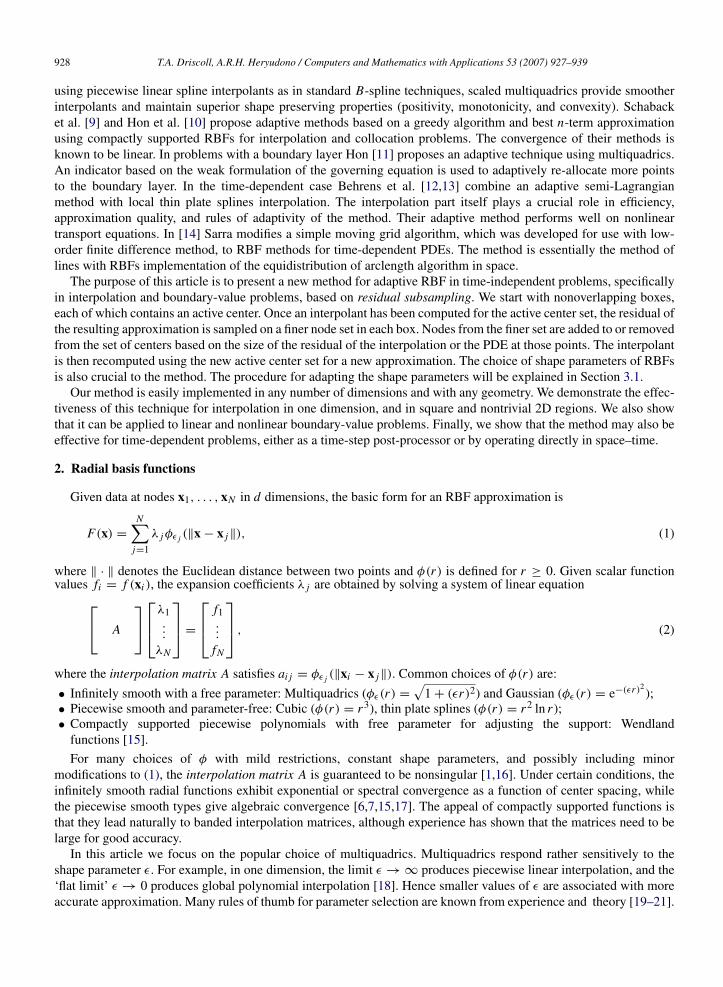
In this section, we describe a simple, easily implemented method for adapting RBF centers and parameters basedon the results of the interpolation process. We call our method residual subsampling. In order to introduce the method,we pick a simple 1D interpolation problem using Runge function f (x) = (25x2
+ 1)−1 on the interval [−1, 1]. First,we generate an initial discretization using N equally spaced points and find the RBF approximation of the function.Next, we compute the interpolation error at points halfway between the nodes. Points at which the error exceeds athreshold θr are to become centers, and centers that lie between two points whose error is below a smaller thresholdθc are removed. The two end points are always left intact. The shape parameter of each center is chosen based onthe spacing with nearest neighbors, and the RBF approximation is recomputed using the new center set. In short,the adaptation process follows the familiar paradigm of solve–estimate–refine/coarsen until a stopping criterion issatisfied. In MATLAB, this problem can be coded in modest number of lines.
930 T.A. Driscoll, A.R.H. Heryudono / Computers and Mathematics with Applications 53 (2007) 927–939
Fig. 1. Left: Runge function with final RBF node distribution. Right: Error convergence of residual subsampling method compared to standardChebyshev interpolation (dashes).
A version of the code with graphics can be downloaded from [27]. Fig. 1 shows the final result obtained fromrunning the MATLAB code. In this case, the adaptative iteration automatically clusters nodes near the boundaries tocounter oscillations while also resolving regions of high activity adequately. The convergence is evidently spectraland virtually identical to Chebyshev. Although the adaptive method above seems adequate for our example, inthe rest of the paper we describe and use a slightly different version that is more easily generalized to higherdimensions.
3.1. Residual subsampling for interpolation
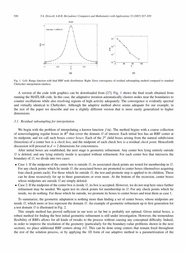
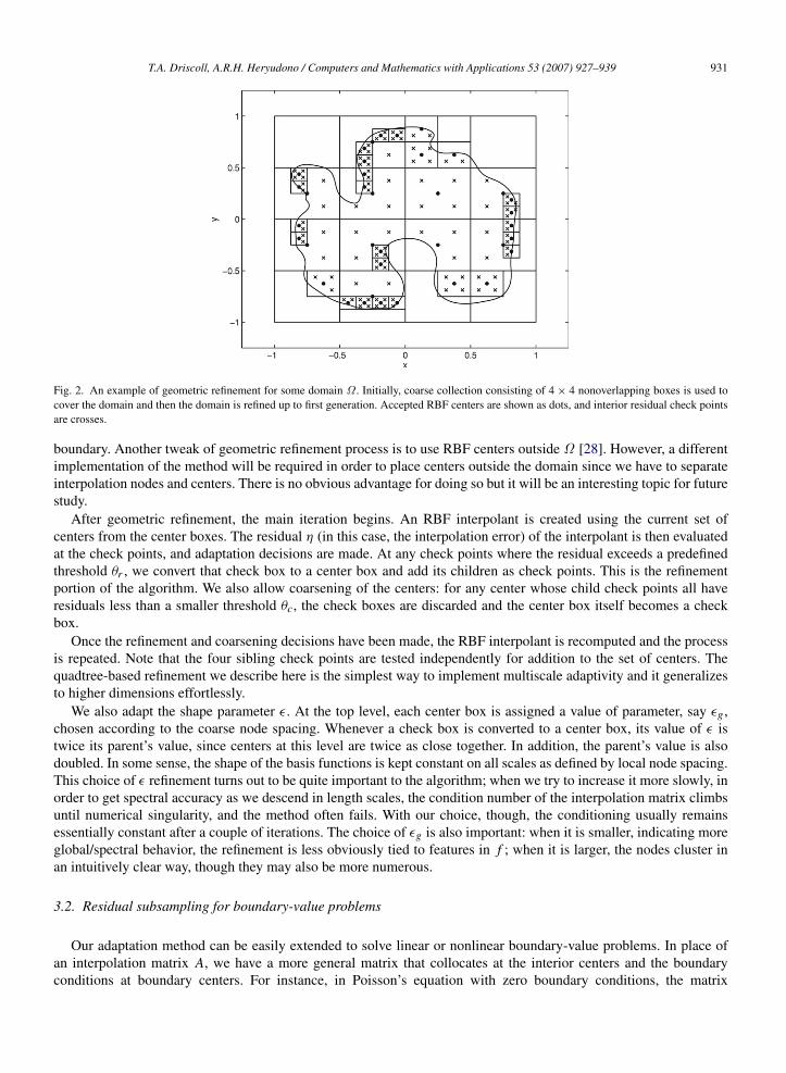
We begin with the problem of interpolating a known function f (x). The method begins with a coarse collectionof nonoverlapping regular boxes in Rd that cover the domain Ω of interest. Each initial box has an RBF center atits midpoint, and we call such boxes center boxes. Each of the 2d child boxes arising from the natural subdivision(bisection) of a center box is a check box, and the midpoint of each check box is a residual check point. Henceforthdiscussion will proceed in d = 2 dimensions for concreteness.
After initial boxes are established, the next stage is geometric refinement. Any center box lying entirely outsideΩ is deleted, and any lying entirely inside is accepted without refinement. For each center box that intersects theboundary of Ω , we divide into two cases:
• Case 1: If the midpoint of the center box is outside Ω , its associated check points are tested for membership in Ω .For any check points which lie inside Ω , the associated boxes are promoted to center boxes (themselves acquiringfour check points each). For those which lie outside Ω , the test-and-promote step is applied to its children. Thesecan be done recursively for up to three generations or even more. At the bottom of the recursion, center boxeswhose midpoints are outside Ω are simply deleted.
• Case 2: If the midpoint of the center box is inside Ω , its box is accepted. However, we do not stop here since furtherrefinement may be needed. We again test its check points for membership in Ω . For any check points which lieinside, we do nothing. For those which lie outside, we promote its boxes to center boxes and treat them as case 1.
To summarize, the geometric adaptation is nothing more than finding a set of center boxes, whose midpoints areinside Ω , which more or less represent the domain Ω . An example of geometric refinement up to first generation fora test domain Ω is illustrated in Fig. 2.
This simple method has proved sufficient in our tests so far but is probably not optimal. Given initial boxes, arobust method for finding the best initial geometric refinement is still under investigation. However, the tremendousflexibility of RBFs allows for all kinds of tweaks to the process without causing any conceptual difficulty. Indeed,in order to improve the resolution of the geometry (particularly for the boundary-value problems shown in the nextsection), we place additional RBF centers along ∂Ω . This can be done using centers that remain fixed throughoutthe rest of the solution process, or by applying the 1D form of our adaptive method to a parametrization of the
T.A. Driscoll, A.R.H. Heryudono / Computers and Mathematics with Applications 53 (2007) 927–939 931
Fig. 2. An example of geometric refinement for some domain Ω . Initially, coarse collection consisting of 4 × 4 nonoverlapping boxes is used tocover the domain and then the domain is refined up to first generation. Accepted RBF centers are shown as dots, and interior residual check pointsare crosses.
boundary. Another tweak of geometric refinement process is to use RBF centers outside Ω [28]. However, a differentimplementation of the method will be required in order to place centers outside the domain since we have to separateinterpolation nodes and centers. There is no obvious advantage for doing so but it will be an interesting topic for futurestudy.
After geometric refinement, the main iteration begins. An RBF interpolant is created using the current set ofcenters from the center boxes. The residual η (in this case, the interpolation error) of the interpolant is then evaluatedat the check points, and adaptation decisions are made. At any check points where the residual exceeds a predefinedthreshold θr , we convert that check box to a center box and add its children as check points. This is the refinementportion of the algorithm. We also allow coarsening of the centers: for any center whose child check points all haveresiduals less than a smaller threshold θc, the check boxes are discarded and the center box itself becomes a checkbox.
Once the refinement and coarsening decisions have been made, the RBF interpolant is recomputed and the processis repeated. Note that the four sibling check points are tested independently for addition to the set of centers. Thequadtree-based refinement we describe here is the simplest way to implement multiscale adaptivity and it generalizesto higher dimensions effortlessly.
We also adapt the shape parameter ε. At the top level, each center box is assigned a value of parameter, say εg ,chosen according to the coarse node spacing. Whenever a check box is converted to a center box, its value of ε istwice its parent’s value, since centers at this level are twice as close together. In addition, the parent’s value is alsodoubled. In some sense, the shape of the basis functions is kept constant on all scales as defined by local node spacing.This choice of ε refinement turns out to be quite important to the algorithm; when we try to increase it more slowly, inorder to get spectral accuracy as we descend in length scales, the condition number of the interpolation matrix climbsuntil numerical singularity, and the method often fails. With our choice, though, the conditioning usually remainsessentially constant after a couple of iterations. The choice of εg is also important: when it is smaller, indicating moreglobal/spectral behavior, the refinement is less obviously tied to features in f ; when it is larger, the nodes cluster inan intuitively clear way, though they may also be more numerous.
3.2. Residual subsampling for boundary-value problems
Our adaptation method can be easily extended to solve linear or nonlinear boundary-value problems. In place ofan interpolation matrix A, we have a more general matrix that collocates at the interior centers and the boundaryconditions at boundary centers. For instance, in Poisson’s equation with zero boundary conditions, the matrix
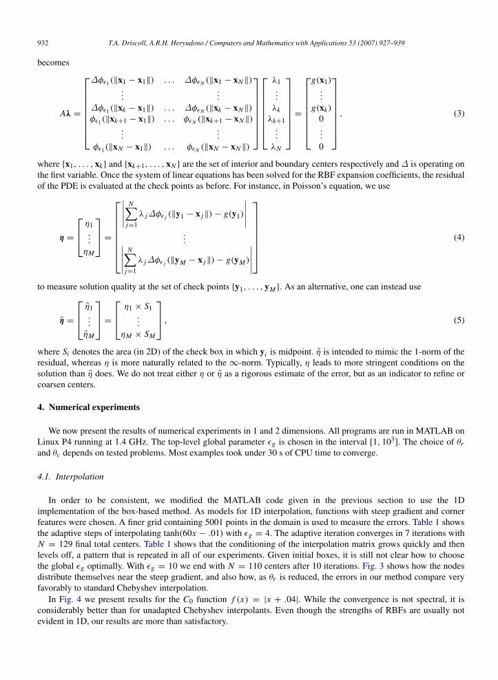
932 T.A. Driscoll, A.R.H. Heryudono / Computers and Mathematics with Applications 53 (2007) 927–939
becomes
Aλ =
∆φε1(‖x1 − x1‖) . . . ∆φεN (‖x1 − xN ‖)...
...
∆φε1(‖xk − x1‖) . . . ∆φεN (‖xk − xN ‖)
φε1(‖xk+1 − x1‖) . . . φεN (‖xk+1 − xN ‖)...
...
φε1(‖xN − x1‖) . . . φεN (‖xN − xN ‖)
λ1...
λkλk+1
...
λN
=
g(x1)...
g(xk)
0...
0
, (3)
where x1, . . . , xk and xk+1, . . . , xN are the set of interior and boundary centers respectively and ∆ is operating onthe first variable. Once the system of linear equations has been solved for the RBF expansion coefficients, the residualof the PDE is evaluated at the check points as before. For instance, in Poisson’s equation, we use
η =
η1...
ηM
=
∣∣∣∣∣ N∑j=1
λ j∆φε j (‖y1 − x j‖) − g(y1)
∣∣∣∣∣...∣∣∣∣∣ N∑
j=1
λ j∆φε j (‖yM − x j‖) − g(yM )
∣∣∣∣∣
(4)
to measure solution quality at the set of check points y1, . . . , yM . As an alternative, one can instead use
η =
η1...
ηM
=
η1 × S1...
ηM × SM
, (5)
where Si denotes the area (in 2D) of the check box in which yi is midpoint. η is intended to mimic the 1-norm of theresidual, whereas η is more naturally related to the ∞-norm. Typically, η leads to more stringent conditions on thesolution than η does. We do not treat either η or η as a rigorous estimate of the error, but as an indicator to refine orcoarsen centers.
4. Numerical experiments
We now present the results of numerical experiments in 1 and 2 dimensions. All programs are run in MATLAB onLinux P4 running at 1.4 GHz. The top-level global parameter εg is chosen in the interval [1, 103
]. The choice of θrand θc depends on tested problems. Most examples took under 30 s of CPU time to converge.
4.1. Interpolation
In order to be consistent, we modified the MATLAB code given in the previous section to use the 1Dimplementation of the box-based method. As models for 1D interpolation, functions with steep gradient and cornerfeatures were chosen. A finer grid containing 5001 points in the domain is used to measure the errors. Table 1 showsthe adaptive steps of interpolating tanh(60x − .01) with εg = 4. The adaptive iteration converges in 7 iterations withN = 129 final total centers. Table 1 shows that the conditioning of the interpolation matrix grows quickly and thenlevels off, a pattern that is repeated in all of our experiments. Given initial boxes, it is still not clear how to choosethe global εg optimally. With εg = 10 we end with N = 110 centers after 10 iterations. Fig. 3 shows how the nodesdistribute themselves near the steep gradient, and also how, as θr is reduced, the errors in our method compare veryfavorably to standard Chebyshev interpolation.
In Fig. 4 we present results for the C0 function f (x) = |x + .04|. While the convergence is not spectral, it isconsiderably better than for unadapted Chebyshev interpolants. Even though the strengths of RBFs are usually notevident in 1D, our results are more than satisfactory.

T.A. Driscoll, A.R.H. Heryudono / Computers and Mathematics with Applications 53 (2007) 927–939 933
Table 1Iterative progress of the refinement algorithm for interpolation of tanh(60x − 0.1)
It N Nc Nr κ(A) ‖.‖∞
1 11 0 18 5.090e+02 7.9211e−012 29 0 34 2.632e+04 4.1501e−013 63 0 31 4.545e+05 1.2544e−014 94 3 30 4.330e+06 1.1129e−025 121 4 12 3.962e+07 2.6766e−046 129 2 2 3.180e+08 5.7980e−057 129 0 0 3.038e+08 2.5329e−05
Nr , Nc = Number of centers to be added/removed respectively.
Fig. 3. Left: tanh(60x − .01). Right: Error convergence of residual subsampling method compared to standard Chebyshev interpolation (dashes).
Fig. 4. Left: |x + .04|, the box-based method adaptively refines centers around corners. Right: Error convergence of residual subsampling methodcompared to standard Chebyshev interpolation (dashes).
Now we move on to 2D cases. In addition to adapting interior points, we also adapt points on the boundary. Our firsttest is with the Franke-type function [29] in [−1, 1]
2, which has been used many times to test for RBF interpolation:
f (x, y) = e−0.1(x2+y2)
+ e−5((x−0.5)+(y−0.5)2)+ e−15((x+0.2)2
+(y+0.4)2)+ e−9((x+0.8)2
+(y−0.8)2), (6)
modified by introducing a singularity of lower-order derivatives along the line y − x = −1 by taking f (x, y) −
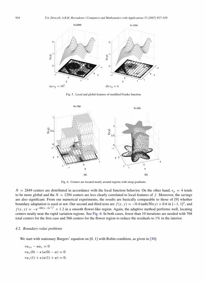
(y − x + 1)y instead of f (x, y) for y − x < −1, see [9]. Only six iterations are needed in reaching the desiredresiduals 8.82 × 10⁻⁴ in interior and 4.24 × 10⁻⁵ on boundary for both εg = 102 and εg = 4. As can be seen fromFig. 5, the two versions look quite different. When εg = 102, the multiquadrics are far from spectral and the final
934 T.A. Driscoll, A.R.H. Heryudono / Computers and Mathematics with Applications 53 (2007) 927–939
(a) εg = 102. (b) εg = 4.
Fig. 5. Local and global features of modified Franke function.
Fig. 6. Centers are located neatly around regions with steep gradients.
N = 2849 centers are distributed in accordance with the local function behavior. On the other hand, εg = 4 tendsto be more global and the N = 1294 centers are less clearly correlated to local features of f . Moreover, the savingsare also significant. From our numerical experiments, the results are basically comparable to those of [9] whetherboundary adaptation is used or not. Our second and third tests are f (x, y) = −0.4 tanh(50xy) + 0.6 in [−1, 1]
2, andf (x, y) = −e−60(y−2x2)2
+ 1.2 in a smooth flower-like region. Again, the adaptive method performs well, locatingcenters neatly near the rapid variation regions. See Fig. 6. In both cases, fewer than 10 iterations are needed with 768total centers for the first case and 566 centers for the flower region to reduce the residuals to 1% in the interior.
4.2. Boundary-value problems
We start with stationary Burgers’ equation on [0, 1] with Robin condition, as given in [30]:
νuxx − uux = 0νux (0) − κ(u(0) − α) = 0νux (1) + κ(u(1) + α) = 0,
T.A. Driscoll, A.R.H. Heryudono / Computers and Mathematics with Applications 53 (2007) 927–939 935
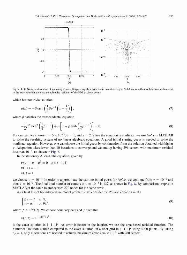
Fig. 7. Left: Numerical solution of stationary viscous Burgers’ equation with Robin condition. Right: Solid lines are the absolute error with respectto the exact solution and dots are pointwise residuals of the PDE at check points.
which has nontrivial solution
u(x) = −β tanh(
12βν−1
(x −
12
)), (7)
where β satisfies the transcendental equation
−12β2 sech2
(14βν−1
)+ κ
[α − β tanh
(14βν−1
)]= 0. (8)
For our test, we choose ν = 5 × 10⁻³, α = 1, and κ = 2. Since the equation is nonlinear, we use fsolve in MATLABto solve the resulting system of nonlinear algebraic equations. A good initial starting guess is needed to solve thenonlinear equation. However, one can choose the initial guess by continuation from the solution obtained with higherν. Adaptation takes fewer than 10 iterations to converge and we end up having 396 centers with maximum residualless than 10−4, as shown in Fig. 7.
In the stationary Allen–Cahn equation, given by
νuxx + u − u3= 0 x ∈ (−1, 1)
u(−1) = −1u(1) = 1,
we choose ν = 10−4. In order to approximate the starting initial guess for fsolve, we continue from ν = 10−2 andthen ν = 10−3. The final total number of centers at ν = 10−4 is 132, as shown in Fig. 8. By comparison, bvp4c inMATLAB at the same tolerance uses 270 nodes for the same error.
As a final test of boundary-value model problems, we consider the Poisson equation in 2D∆u = f in Ω ,
u = uo on ∂Ω ,(9)
where f ∈ C∞(Ω). We choose boundary data and f such that
u(x, t) = e−10(x2+y2) (10)
is the exact solution in [−1, 1]2. As error indicator in the interior, we use the area-based residual function. The
numerical solution is then compared to the exact solution on a finer grid in [−1, 1]2 using 4000 points. By taking
εg = 1, only 4 iterations are needed to achieve maximum error 4.54 × 10⁻⁵ with 260 centers.

936 T.A. Driscoll, A.R.H. Heryudono / Computers and Mathematics with Applications 53 (2007) 927–939
Fig. 8. Numerical solution of stationary Allen–Cahn with parameter ν = 10−4.
Fig. 9. Numerical solution of Poisson’s equation in starfish-like domain.
For a more complicated domain, like the smooth “starfish” in Fig. 9, we use forcing term f (x, y) =
100e−200(x2+y2). With εg = 4, Fig. 9 shows the solution after 3 iterations. Note that we measure the Dirichlet boundary
residuals as well as Laplace residuals inside the domain. Usually these residuals differ in orders of magnitude.Following [10], we calculate their relative magnitude and introduce a weighted maximum norm which often putsa larger weight on the quality of the boundary values.
The final test is the L-shaped domain with the forcing term
f (x, y) = −10e−10((x−0.1)2+(y−0.1)2)
close to the corner, as shown in Fig. 10. The iteration stops successfully with N = 2100. We do not regard automaticadaptation as the ideal method for a singularity due to a geometric corner. One would probably do much better withan a priori adaptation or by including appropriate singular functions in the interpolant [31].
4.3. Time-dependent problems
One way to use our adaptation in a time-dependent problem is to alternate time stepping with adaptation. Inthis model, an initial condition at t = 0 is used to adaptively select the RBF nodes and shape parameters. Theseparameters define a standard method-of-lines semi-discretization that can be used to advance the discrete solution upto a predetermined time t = τ . Now that one has values at the RBF nodes that implicitly determine an RBF interpolantapproximating the solution at t = τ , we can apply the residual subsampling algorithm to the interpolant to derive anew set of RBF nodes and shape parameters. This is treated like a new initial state for further time stepping, etc. The

T.A. Driscoll, A.R.H. Heryudono / Computers and Mathematics with Applications 53 (2007) 927–939 937
Fig. 10. Numerical solution of Poisson’s equation in L-shaped domain.
Fig. 11. Solution of the Allen–Cahn equation (11) using a model of alternating time stepping and adaptation by residual subsampling of theapproximate solution. Each line in the figure represents a time at which adaptation has occurred. The nodes clearly adapt themselves to emergingsteep gradients.
idea is to pick τ large enough to avoid excessive adaptation steps, while keeping it small enough that the adaptationcan keep up with emerging or changing features in the solution.
Fig. 11 shows the result of this alternating model for the Allen–Cahn equation,
ut − u(1 − u2) = νuxx , (11)
with ν = 10−6, u(±1, t) = ±1, and u(x, 0) = 0.6x + 0.4 sin[
π2 (x2
− 3x − 1)]. The solution is advanced in
time using fourth-order Runge–Kutta with step size 0.01, and adaptation occurs every 25 time steps with thresholdsθr = 200θc = 10−3. The number of RBF nodes starts with 27 and gradually grows to a maximum of 178 at t = 8.25.As the figure shows, the nodes are able to track the developing steep gradients quite efficiently.
Our final example is the moving front problem given by the Burgers’ equation
νuxx − uux = ut , 0 < x < 1u(0, t) = u(1, t) = 0
u(x, 0) = sin(2πx) +12
sin(πx).
This problem is known to be a common test problem for many adaptive methods [32]. The solution generates asteep front with width O(ν) moving towards x = 1 which also decays with time due to the boundary conditions.

938 T.A. Driscoll, A.R.H. Heryudono / Computers and Mathematics with Applications 53 (2007) 927–939
Fig. 12. Solution of the Burgers’ equation using a model of alternating time stepping and adaptation by residual subsampling of the approximatesolution. Each line in the figure represents a time at which adaptation has occurred.
Fig. 13. Numerical solution of time-dependent Burgers’ equation using direct implementation of residual subsampling method in space–time.
Our numerical experiment was run with ν = 10−3. The solution is advanced in time using MATLAB built-in stiffodesolver ode15s. As Fig. 12 shows, the nodes are able to track the developing moving front. As an alternative tostep-and-adapt method, our numerical experiment can be run directly in space–time. In other words, we treat thisspace–time problem as a regular 2D case. The choice of the distance function is the Euclidean distance in space–timegiven by
r =
√(x − x j )2 + (t − t j )2. (12)
To start with, we compute Burgers’ equation in the space–time slab [0, 1] × [0, 2]. We apply boundary adaptationexcept at points with t = 0.2 and the area-based residuals are used as error indicator. We use fsolve in MATLAB tosolve the nonlinear equations with u(x, t) = sin(2πx) +
12 sin(πx), where t = [0, 0.2] as the surface of the very
first initial guess. Even though fsolve has a built-in feature based on finite difference to calculate the Jacobian of thenonlinear algebraic equations, in this case we are able to use the exact Jacobian. The residuals are less than 5 × 10⁻⁴
in fewer than 10 adaptive iterations. In Fig. 13, we can see that the RBF centers are adaptively located following thepath of the moving front problem.
The process of marching in time can be done in a straightforward manner. Once we found all information such ascenters, shape parameters, and values at current space–time slab, we simply apply the same adaptive technique to thenext slab by using the values at final previous time as a new initial condition. In this preliminary form, the application
T.A. Driscoll, A.R.H. Heryudono / Computers and Mathematics with Applications 53 (2007) 927–939 939
of residual subsampling in time-dependent problems is very promising. However, the stability and robustness of themethod in time-dependent cases are still under research.
References
[1] M.D. Buhmann, Radial Basis Functions: Theory and Implementations, in: Cambridge Monographs on Applied and ComputationalMathematics, vol. 12, Cambridge University Press, Cambridge, 2003.
[2] E.J. Kansa, Multiquadrics—A scattered data approximation scheme with applications to computational fluid-dynamics. I. Surfaceapproximations and partial derivative estimates, Comput. Math. Appl. 19 (8–9) (1990) 127–145.
[3] E.J. Kansa, Multiquadrics—A scattered data approximation scheme with applications to computational fluid-dynamics. II. Solutions toparabolic, hyperbolic and elliptic partial differential equations, Comput. Math. Appl. 19 (8–9) (1990) 147–161.
[4] C. Franke, R. Schaback, Solving partial differential equations by collocation using radial basis functions, Appl. Math. Comput. 93 (1) (1998)73–82.
[5] E. Larsson, B. Fornberg, A numerical study of some radial basis function based solution methods for elliptic PDEs, Comput. Math. Appl. 46(5–6) (2003) 891–902.
[6] A.H.-D. Cheng, M.A. Golberg, E.J. Kansa, G. Zammito, Exponential convergence and h-c multiquadric collocation method for partialdifferential equations, Numer. Methods Partial Differential Equations 19 (5) (2003) 571–594.
[7] M. Buhmann, N. Dyn, Spectral convergence of multiquadric interpolation, Proc. Edinb. Math. Soc. (2) 36 (2) (1993) 319–333.[8] M. Bozzini, L. Lenarduzzi, R. Schaback, Adaptive interpolation by scaled multiquadrics, Adv. Comput. Math. 16 (4) (2002) 375–387.[9] R. Schaback, H. Wendland, Adaptive greedy techniques for approximate solution of large RBF systems, Numer. Algorithms 24 (3) (2000)
239–254.[10] Y.C. Hon, R. Schaback, X. Zhou, An adaptive greedy algorithm for solving large RBF collocation problems, Numer. Algorithms 32 (1) (2003)
13–25.[11] Y.C. Hon, Multiquadric collocation method with adaptive technique for problems with boundary layer, Internat. J. Appl. Sci. Comput. 6 (3)
(1999) 173–184.[12] J. Behrens, A. Iske, M. Kaser, Adaptive meshfree method of backward characteristics for nonlinear transport equations, in: Meshfree Methods
for Partial Differential Equations (Bonn, 2001), in: Lect. Notes Comput. Sci. Eng., vol. 26, Springer, Berlin, 2003, pp. 21–36.[13] J. Behrens, A. Iske, Grid-free adaptive semi-Lagrangian advection using radial basis functions, Comput. Math. Appl. 43 (3–5) (2002) 319–327.[14] S.A. Sarra, Adaptive radial basis function methods for time dependent partial differential equations, Appl. Numer. Math. 54 (1) (2005) 79–94.[15] H. Wendland, Piecewise polynomial, positive definite and compactly supported radial functions of minimal degree, Adv. Comput. Math. 4 (4)
(1995) 389–396.[16] C.A. Micchelli, Interpolation of scattered data: Distance matrices and conditionally positive definite functions, Constr. Approx. 2 (1) (1986)
11–22.[17] J. Yoon, Spectral approximation orders of radial basis function interpolation on the Sobolev space, SIAM J. Math. Anal. 33 (4) (2001) 946–958
(Electronic).[18] T.A. Driscoll, B. Fornberg, Interpolation in the limit of increasingly flat radial basis functions, Comput. Math. Appl. 43 (3–5) (2002) 413–422.[19] E.J. Kansa, R.E. Carlson, Improved accuracy of multiquadric interpolation using variable shape parameters, Comput. Math. Appl. 24 (12)
(1992) 99–120.[20] R.E. Carlson, T.A. Foley, The parameter R2 in multiquadric interpolation, Comput. Math. Appl. 21 (9) (1991) 29–42.[21] S. Rippa, An algorithm for selecting a good value for the parameter c in radial basis function interpolation, Adv. Comput. Math. 11 (2–3)
(1999) 193–210.[22] R. Schaback, Error estimates and condition numbers for radial basis function interpolation, Adv. Comput. Math. 3 (3) (1995) 251–264.[23] B. Fornberg, G. Wright, Stable computation of multiquadric interpolants for all values of the shape parameter, Comput. Math. Appl. 48 (5–6)
(2004) 853–867.[24] R.K. Beatson, J.B. Cherrie, C.T. Mouat, Fast fitting of radial basis functions: Methods based on preconditioned GMRES iteration, Adv.
Comput. Math. 11 (2–3) (1999) 253–270.[25] R.B. Platte, T.A. Driscoll, Polynomials and potential theory for Gaussian radial basis function interpolation, SIAM J. Numer. Anal. 43 (2)
(2005) 750–766 (Electronic).[26] B. Fornberg, T.A. Driscoll, G. Wright, R. Charles, Observations on the behavior of radial basis function approximations near boundaries,
Comput. Math. Appl. 43 (3–5) (2002) 473–490.[27] T.A. Driscoll, http://www.math.udel.edu/˜driscoll/index.html.[28] A.I. Fedoseyev, M.J. Friedman, E.J. Kansa, Improved multiquadric method for elliptic partial differential equations via PDE collocation on
the boundary, Comput. Math. Appl. 43 (3–5) (2002) 439–455.[29] R. Franke, Scattered data interpolation: Tests of some methods, Math. Comp. 38 (157) (1982) 181–200.[30] L.G. Reyna, M.J. Ward, On the exponentially slow motion of a viscous shock, Comm. Pure Appl. Math. 48 (2) (1995) 79–120.[31] R.B. Platte, T.A. Driscoll, Computing eigenmodes of elliptic operators using radial basis functions, Comput. Math. Appl. 48 (3–4) (2004)
561–576.[32] W. Huang, Y. Ren, R.D. Russell, Moving mesh methods based on moving mesh partial differential equations, J. Comput. Phys. 113 (2) (1994)
279–290.