collocation impacts on the vulnerability of lifelines ... · collocation impacts on the...
TRANSCRIPT

FEDERAL EMERGENCY MANAGEMENT AGENCY
Collocation Impacts on theVulnerability of Lifelines DuringEarthquakes with Applictions tothe Cajon Pass, California
Issued in Furtherance of the Decadefor Natural Disaster Reduction
Earthquake Hazard Reduction Series 61
FEMA 2261 February 1992

Collocation Impacts on theVulnerability of Lifelines During
Earthquakes with Applications to theCajon Pass, California
Submitted to the Federal Emergency Management AgencyWashington, D.C.
Submitted by:
INTECH Inc.11316 Rouen Dr.
Potomac, MD 20854-3126
Co-Principal Investigators:Dr. Phillip A. Lowe, INTEC, Inc.
Dr. Charles F. Scheffey, INTEC, Inc.Mr. Po Lam, Earth Mechanics, Inc.

COLLOCATION IMPACTS ON THE VULNERABILITY OF LIFELINES DURING
EARTHQUAKES WITH APPLICATION TO THE CAJON PASS, CALIFORNIA
TABLE OF CONTENTSVolume 1
ITEM PAGE
Table of Contents ..................... t .i
List of Figure............................................ ii
List of Tables........................................ v
1.0 CONCLUSIONS ................................... 1
2.0 INTRODUCTION ..................... . . 4
2.1 Background .. . ...... 4
2.2 Study Approach . . .................... . . 5
2.3 Chapter 2.0 Bibliography ................................ 6
3.0 SUMMARY .................................. . 6
4.0 ANALYSIS METHOD ...................................... 8
4.1 Data Acquisition . . . ............. 11
Lifeline and Geologic Information ... . . 11
Ground Shaking Intensity . . ............................... 13
Selection of the Earthquake Event ...................... 16
4.2 Calculation of Lifeline vulnerability .................. 16
Damage Assessment ................................... . 16
Shaking Damage .. . ..... 18
Fault Displacement. . . 23
Soil Movement . . ........................................ 24
Landslide .... 24
Liquefaction or Lateral Spread . . . .30
Highway and Railway Bridges . . ... 31
Times, to Restore the Lifeline to its Needed Service 37
Repair Time .............. 37
Access Time .... 38
Equipment and Material Time ........................... 39
4.3 Collocation Analysis .................................... 39
Impacts on Damage State....... .... 42
Impacts on Probability of Damage .... 42
Impacts on Time to Restore Lifeline Service . .43
4.4 Interpretation of the Results. .......................... 44
4.5 -Chapter 4.0 Bibliography ............................... 45
5.0 APPLICATION OF THE METHOD TO CAJON PASS ........ 47
5.1 Data Acquisition .... 47
5.2 Lifeline Collocation Vulnerability Analysis Results 55
Communication Lifelines .... 61
Electric Power Lifelines . . ............................ 6.8
Fuel Pipeline Lifelines ............................... 75
Transportation Lifelines .... 81
5.3 Chapter 5.0 Bibliography. . . 91
6.0 FUTURE STUDY NEEDS .... 91
Appendix A Modified Mercalli Intensity (MMI) Index Scale
i

LIST OF FIGURES
FIGURE PAGE
1 Flow Chart of the Analysis Method ....................
2 The "Attenuation Parameter k" for Use in CalculatingEarthquake Shaking Intensity .........................
3 Map of the U.S. Seismic Hazard Regions ................
4 Liquefaction Induced Damage ...........................
9
15
22
32
5 Map Showing the General Location of the CajonPass Study Area ....................................... 48
6 A Composite of the Lifeline Routes at Cajon Pass ...... 50
7 Identification of Collocations At Cajon Pass ... ....... 52
8 Lifeline Routes With Shaking Intensity andPotential Landslide and Liquefaction Areas ... ......... 54
9 Communication Lifeline Routes .......................... 62
10 Fiber Optic Conduits On A Bridge On The AbandonedPortion of Cajon Blvd. Extension ...................... 63
11 Details of the Fiber Optic Conduits of Figure 10 ...... 63
12 Fiber Optic Conduits On A Concrete CulvertThat Passes Under I-15 ................................ 64
13 Wall Support Details for the Fiber Optic ConduitsShown in Figure 12 .................................... 64
14 Surface Water Conditions Near The Toe of The I-15SRetaining Crib Wall ................................... 65
15 Fiber Optic Conduits Under a Heavy Water Pipe, Bothon a Highway Bridge ................................... 65
16 Electric Power Lifeline Routes ........................ 69
17 A Landslide Scar With Power Towers in the Slide Area .. 70
18 Power Lines, Natural Gas and Petroleum Products PipelinesIntersecting Over the San Andreas Fault Rift Zone ..... 71
ii
Figure
Figure
Figure
Figure
Figure
Figure
Figure
Figure
Figure
Figure
Figure
Figure
Figure
Figure
Figure
Figure
Figure
Figure

Figure 19 Power Tower at a Ravine Edge in the San Andreas FaultRift Zone .............. 72
Figure 20 Fuel Pipeline Lifeline Routes ...................... 76
Figure 21 Typical Long Open Span on the 36-Inch Natural
Gas Pipeline ...................................... 75
Figure 22 Two Natural Gas Pipelines Located Next to Highway 138 . 77
Figure 23 Natural Gas Pipeline Crossing Under Railroad Beds . 78
Figure 24 Transportation Lifeline Routes .......................... 83
Figure 25 I-15 Bridge Over Railroads in Cajon Wash .............. 84
Figure 26 I-15 Bridge Over Cajon Wash .................... ........ 84
Figure 27 Highway 138 Bridge Over I-15 .......................... 85
Figure 28 Railroad Bridges in Cajon Wash (I-15 Bridge in
Background) ................................... 86.... 8
Figure 29 Railroad Bridge Over Highway 138 (Collapse Expected) .. 86
Figure 30 Santa Fe Railroad Bubble Masonry Pier Bridge .8........ 87
Figure 31 Union Pacific Railroad Bridge With Power Lines
Overhead.....................................8....... 7
Figure 32 Typical I-15 Box Bridge Over the Railroads .90
Figure 33 I-15 and Access Road Bridges Over the SouthernPacific Railroad .............. 90..............I ...... 90
iii
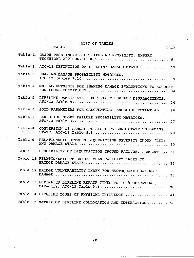
LIST OF TABLESTABLE PAGE
Table 1. CAJON PASS IMPACTS OF LIFELINE PROXIMITY: EXPERTTECHNICAL ADVISORY GROUP .............................. 6
Table 2. ATC-13 DEFINITION OF LIFELINE DAMAGE STATE ... ......... 17
Table 3 SHAKING DAMAGE PROBABILITY MATRICES,ATC-13 Tables 7.10 .................................... 19
Table 4 MMI ADJUSTMENTS FOR SHAKING DAMAGE EVALUATIONS TO ACCOUNTFOR LOCAL CONDITIONS .................................. 23
Table 5 LIFELINE DAMAGE STATE FOR FAULT SURFACE DISPLACEMENTS,ATC-13 Table 8.9 ...................................... 24
Table 6 SOIL PARAMETERS FOR CALCULATING LANDSLIDE POTENTIAL ... 26
Table 7 LANDSLIDE SLOPE FAILURE PROBABILITY MATRICES,ATC-13 Table 8.7 ...................................... 27
Table 8 CONVERSION OF LANDSLIDE SLOPE FAILURE STATE TO DAMAGESTATE, ATC-13 Table 8.8 ................................ 29
Table 9 RELATIONSHIP BETWEEN LIQUEFACTION SEVERITY INDEX (LSI)AND DAMAGE STATE ...................................... 30
Table 10 PROBABILITY OF LIQUEFACTION GROUND FAILURE, PERCENT ... 31
Table 11 RELATIONSHIP OF BRIDGE VULNERABILITY INDEX TOBRIDGE DAMAGE STATE ................................... 33
Table 12 BRIDGE VULNERABILITY INDEX FOR EARTHQUAKE SHAKINGDAMAGE ................................................ 35
Table 13 ESTIMATED LIFELINE REPAIR TIMES TO 100% OPERATINGCAPACITY, ATC-13 Table 9.11 ........................... 38
Table 14 LIFELINE ZONES OF PHYSICAL INFLUENCE .................. 41
Table 15 MATRIX OF LIFELINE COLLOCATION AND INTERACTIONS ....... 56
iv
COLLOCATION IMPACTS ON THE VULNERABILITY OF LIFELINES DURING
EARTHQUAKES WITH APPLICATION TO THE CAJON PASS, CALIFORNIA
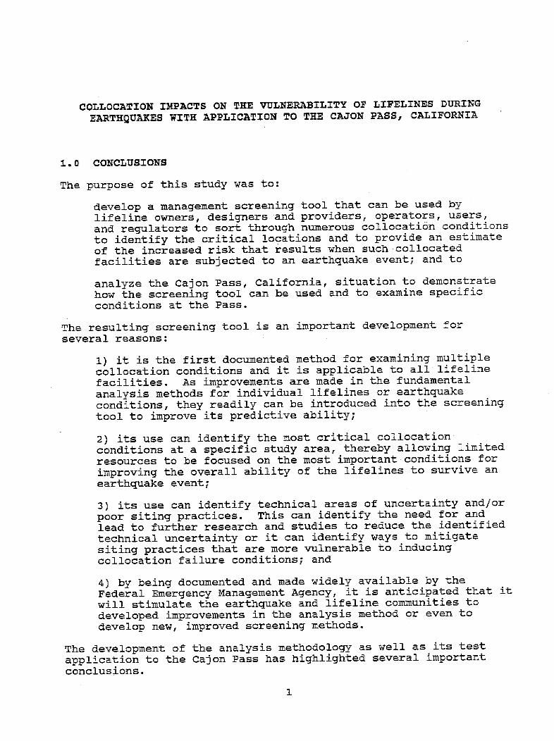
1.0 CONCLUSIONS
The purpose of this study was to:
develop a management screening tool that can be used bylifeline owners, designers and providers, operators, users,and regulators to sort through numerous collocation conditions
to identify the critical locations and to provide an estimateof the increased risk that results when such collocatedfacilities are subjected to an earthquake event; and to
analyze the Cajon Pass, California, situation to demonstratehow the screening tool can be used and to examine specificconditions at the Pass.
The resulting screening tool is an important development forseveral reasons:
1) it is the first documented method for examining multiplecollocation conditions and it is applicable to all lifeline
facilities. As improvements are made in the fundamental
analysis methods for individual lifelines or earthquakeconditions, they readily can be introduced into the screeningtool to improve its predictive ability;
2) its use can identify the most critical collocationconditions at a specific study area, thereby allowing limitedresources to be focused on the most important conditions forimproving the overall ability of the lifelines to survive anearthquake event;
3) its use can identify technical areas of uncertainty and/orpoor siting practices. This can identify the need for andlead to further research and studies to reduce the identifiedtechnical uncertainty or it can identify ways to mitigatesiting practices that are more vulnerable to inducingcollocation failure conditions; and
4) by being documented and made widely available by theFederal Emergency Management Agency, it is anticipated that itwill stimulate the earthquake and lifeline communities todeveloped improvements in the analysis method or even todevelop new, improved screening methods.
The development of the analysis methodology as well as, its testapplication to the Cajon Pass has highlighted several importantconclusions.
I

o Lifeline collocation can produce both benefits and increasedrisk of failure during earthquake events. A benefit ofclosely located transportation lifelines is that the secondlifeline can provide the detour or access route to the damagedsections of the first lifeline. However, intersectinglifelines generally result in the failure of one lifelineincreasing the risk of failure of the lifeline(s) it crosses.
o It is understandable that topographic conditions have led tothe routing of lifeline systems in corridors. However,manmade considerations that force the lifeline owners to usethe same rights-of-way for widely different lifelines (forexample, locating petroleum fuel pipeline and communicationconduits next to each other, routing natural gas pipelinesback and forth under a railroad bed, and having a mix oflifelines cross the earthquake fault zone at the samelocation) greatly increase the risk of failure for theindividual lifelines and the complications that will beencountered during site restoration after an earthquake.
o As compared to buildings, ground movement is more importantthat ground shaking for lifeline components, especially buriedlifelines and electrical transmission towers. This means thatmuch of the technical data base on earthquake shakingintensity is not critical for lifeline analysis, whereasimportant ground movement data and analyses are not as welldeveloped as the shaking intensity data. This suggests thatfuture studies need to emphasize obtaining ground movementinformation.
o A very useful screening tool has been developed during thisstudy. The tool can be used to identify the critical lifelinecollocation locations and the conditions that make themcritical. It can identify areas of technical uncertainty andpoor siting practices, and its use can identify importantresearch and development activities that can lead to loweredrisk of collocation-induced lifeline failures. It will be ofvalue to lifeline owners, designers and providers, operators,users, and regulators.
o The analysis tool has been successfully applied to the CajonPass, California. It has identified that for this semi-desertregion that:
The Cajon Junction, Lone Pine Canyon (which contains theSan Andreas fault zone), Blue Cut, and the area justsouth of the interchange between I-15 and I-215 are thecritical locations in terms of collocation impacts at theCajon Pass.
Fuel pipeline failures have the greatest impact on theother lifelines during the immediate recovery period
2

after an earthquake.
Current siting practices for fiber optic cables indicates
that more severe telephone communication failures than
have been experienced in past earthquakes can be
anticipated in future earthquakes when fiber optic
systems have become more dominant in providing the basic
telephone service.
Lifeline siting practices have not fully considered the
impacts that a new lifeline will have on existing
lifelines and, conversely, the impacts that the existing
lifelines will have on the new lifeline.
Transportation lifeline restoration of service is highly
dependent on sequentially repairing the lifeline damage
as the lifeline itself is needed to provide access to the
next damage location. Parallel repair operations are
more probable for the other lifeline systems.
Communication, electric power, and fuel pipeline
lifelines can generally be analyzed as a set of discrete
collocation points. The restoration of service at any
one point is not a strong function of the restoration
work that is needed at other collocation points. Thus,
if there is a restoration problem that will take a long
time compared to the other locations, it becomes the
"critical path" that sets the time period for the
restoration of the entire lifeline system.
When multiple lifelines of the same class are collocated
(such as installing all fiber optic cables or all fuel
pipelines in the same or parallel trenches) or when
multiple different lifelines intersect at a common point,
the reliability of each individual lifeline decreases to
the value of the "weakest link" of the combined lifeline
systems. In addition, repair times increase because of
local congestion and the concern that work on one
lifeline component could lead to damage of the other
different lifeline components.
o There is a need for further collocation lifeline studies: to
apply the newly developed screening tool to other locations to
assure that the methods can be transferred to other U.S.
locations and to analyze different lifelines, geographic, and
earthquake conditions; and to develop data and approaches that
can be used to further improve the predictive capabilities of
the screening tool.
3

2.0 INTRODUCTION
2.1 Background
Lifelines (e.g., systems and facilities that deliver energy andfuel and systems and facilities that provide key services such aswater and sewage, transportation, and communications are defined aslifelines) are presently being sited in "utility or transportationcorridors" to reduce their right-of-way environmental, aesthetic,and cost impacts on the communities that rely upon them. Theindividual lifelines are usually designed, constructed, andmodified throughout their service life. This results in differentstandards and siting criteria being applied to segments of the samelifeline, and also to different standards or siting criteria beingapplied to the separate lifelines systems within a single corridor.Presently, the siting review usually does not consider the impactof proximity or collocation of the lifelines on their individualrisk or vulnerability to natural or manmade hazards or disasters.This is either because the other lifelines have not yet beeninstalled or because such a consideration has not been identifiedas being an important factor for such an evaluation.
There have been cases when some lifeline collocations haveincreased the levels of damage experienced during an accident or anearthquake. For example, water line ruptures during earthquakeshave led to washouts which have caused foundation damage to nearbyfacilities. In southern California a railroad accident(transportation lifeline) led to the subsequent failure of acollocated fuel pipeline, and the resulting fire causedconsiderable property damage and loss of life. Loss of electricpower has restricted, and sometimes failed, the ability to providewater and sewer services or emergency fire fighting capabilities.
In response to these types of situations, the Federal EmergencyManagement Agency (FEMA) is examining the use of such corridors,and FEMA initiated this study to examine the impact of sitingmultiple lifeline systems in confined and at-risk areas.
The overall FEMA project goals are to develop managerial tools thatcan be used to increase the understanding of the lifeline systems'vulnerabilities and to help identify potential mitigationapproaches that could be used to reduce those vulnerabilities.Another program goal is to identify methods to enhance the transferof the resulting information to lifeline system providers,designers, builders, managers, operators, users, and regulators.
This report is the second of a series of three reports. The firstreport(' presented an inventory of the major lifeline systemslocated at Cajon Pass, California, and it summarized the earthquakeand geologic analysis tools available to identify and define the
* The numbers in superscript are references found at the end of eachchapter. 4

level of seismic risk to those lifelines. This report presents theanalytic methods developed to define the collocation impacts andthe resulting analyses of the seismic and geologic environmentalloads on the collocated lifelines in the Cajon Pass. The assumedearthquake event is similar to the 8.3 magnitude, San Andreasfault, Ft. Tejon earthquake of 1857. In this, report a new analysismethod is developed and applied to identify the increase in thevulnerability of the individual lifeline systems due to theirproximity to other lifelines in the Cajon Pass. A third reportspresents an executive summary of the study. The Cajon PassLifeline Inventory report and this present report taken togetherprovide a specific example of how the new analysis method can beapplied to a real lifeline corridor situation.
2.2 Study Approach
The approach used to develop the information for this report was asfollows. The Cajon Lifeline Inventory report('), additionalinformation provided during direct meetings with the lifelineowners, site reconnaissance surveys to validate the information andto examine specific site conditions of interest to the study, andexisting literature that describes lessons learned from actualearthquake events were compiled and thoroughly studied. Theprincipal investigators then hypothesized an analysis method thatcould be applied to the Cajon Pass lifelines to estimate theimpacts of proximity on their earthquake-induced performance andrepairs.
This analysis method emphasizes building upon existing data basesand analytic methods. In applications, it is recommended that theanalyses, studies, and information available from the lifelineowners be used whenever possible. In the event that sufficientdata on the lifeline response to earthquakes and the expected timeto restore the lifeline back to its, required service level are notavailable from the lifeline owners, the analytic methods, with someimportant modifications, of "Earthquake Damage Evaluation Data forCalifornial, ATC-13(3 ), are recommended as an appropriate alternativeanalysis method. In this project the "most probable restorationtime" was defined as the analysis parameter that best could be usedto define the impact of lifeline proximity on the individuallifeline's earthquake vulnerability.
The resulting method was then applied to the Cajon Pass lifelines.The U.S. Geologic Survey's digitized topographic map of the CajcnPass and the contiguous quadrangles were utilized. The commercial,computer aided, design program AutoCAD was used as it is readilyavailable to the public, thus the methodology is not limited tobeing dependent upon a specialized or proprietary computer program.With this tool, overlays of the lifeline routes with seismic andgeologic information presented in the inventory reportcl' were usedto identify the conditions and locations where the individuallifelines were most vulnerable to the hypothesized earthquake. The
5

analysis methods described in Section 4.0 of this report were thenapplied to the lifelines and the results are presented in Section5.0. Section 6.0 identifies future studies that could beundertaken to further qualify the analysis methods and to improvethe details of the specific analysis activities. Section 3.0provides a summary of the study.
As part of the study validation process, the draft results of thestudy were submitted to the project advisors, see Table 1, fortheir independent professional evaluation and to the lifelineowners and regulators who provided information for the preparationof the report or the Cajon Pass Inventory report. FEMA also sentdraft report copies to a select list of independent reviewers.Each comment received was addressed, and this final report then wasprepared and submitted to FEMA.
Table 1CAJON PASS IMPACTS OF LIFELINE PROXIMITY:
EXPERT TECHNICAL ADVISORY GROUP
William S. Bivins T.D. O'RourkeJames H. Gates Dennis K. OstromLe Val Lund Kenneth F. SullivanJohn D. (Jack) McNorgan
2.3 Chapter 2.0 Bibliography
1. P. Lowe, C. Scheffey, and P. Lam, "Inventory of Lifelines inthe Cajon Pass, California", ITI FEMA CP 120190, August 1991.
2. P. Lowe, C. Scheffey, and P. Lam, "Collocation Impacts onLifeline Earthquake Vulnerability at the Cajon Pass, -California, Executive Summary", ITI FEMA CP 050191-ES, August1991.
3. C. Rojahn and R. Sharpe, "Earthquake Damage Evaluation Datafor California", ATC-13, 1985.
3.0 SUMMARY
This report presents a systematic approach to calculate the impactsdue to the collocation or close proximity of one lifeline toanother during earthquake conditions. Specifically, thecollocation vulnerability impact is defined as the increase in themost probable time to restore the lifeline to its intended level ofservice. The analysis methods proposed are intended to be used inscreening analyses that determine which lifelines or lifelinesegments are most impacted by the collocation or close proximity ofother lifelines. Once the critical locations or conditions areknown, it may be equally important to reanalyze them using moredetailed analyses to further define the collocation impacts.
6

The methods proposed are to use the best available information todetermine the lifeline damage state, the probability that thedamage state or greater will occur, and the time to restore thelifeline to its intended service. Normally, such information isobtained from the lifeline owner/operator. However, a alternativemethod is proposed when such information is not available from thatsource.
The alternative method is based on building upon existingearthquake damage information and analysis methods which have been'compiled by the Applied Technology Council (ATC). In that manner,the analysis results can be compared with earlier or future studiesthat use the data base without the need to compare or justify thedata base. However, important improvements to the existing ATCdata base also are presented.
Collocation impacts, can be described in one of two broad terms: 1)the resource impacts (i.e., the increase in personnel, equipment,and material resources) that are required to return the totallifeline system to its needed operating capacity. This isperformed in the present method by summing the impacts at eachcomponent along the entire lifeline route. 2) the resource impactsat a specific location where multiple lifeline components arelocated. In both cases, the present method uses the most probabletime to restore the lifeline component or system to its neededoperating capacity as the appropriate measure of the resourceimpacts.
The analysis method has been applied to the lifeline systems in theCajon Pass, California, as a test case. It is clear that thecommunication, electric power, and fuel transmissions lifelinesystems that have the potential for collocation impacts are, ingeneral, not very sensitive to earthquake ground shaking forshaking intensities represented by Modified Mercalli Intensityindices of VIII or less (these are the values found at Cajon Passfor the assumed earthquake event). They are, however, verysensitive to ground movement expressed as fault displacement,landslides, or lateral spreads. Bridges are sensitive to bothground shaking and ground conditions (displacement, landslide,lateral spread, and local liquefactions at their foundationlocations).
It is understandable that topographic conditions have led to therouting of lifeline systems into corridors. However, manmadeconsiderations that force the lifeline owners to use the exact samerights-of-way for widely different needs (for example, locatingpetroleum fuel pipeline and communication conduits next to eachother, routing natural gas pipelines back and forth under arailroad bed, and having a mix of lifelines cross the earthquakefault zone at the same location) greatly increases the individuallifeline risks and the complications that will be encounteredduring site restoration after an earthquake.
7

The Cajon Pass example has identified that the communication,electric power transmission, and fuel pipeline lifelines generallycan be analyzed as a set of discrete collocation points. Therestoration of service at any one point is not a strong function ofthe restoration work that is needed at other collocation points.Thus, if there is a restoration problem that will take a long timecompared to the other locations, it becomes the "critical path"that sets the time period for the restoration of the entirelifeline system. Transportation lifeline collocation points,however, are sensitive to the damage that has occurred along theroute of the transportation system. That is, often it is necessaryfor the heavy equipment and material needed to have access to thedamage location by traveling along the highway or railroad itself.Thus, before access to a particular bridge can be made, it may benecessary to first repair all the damage sites on the route priorto that location.
4.0 ANALYSIS METHOD
In performing an analysis of the impacts of collocation or closeproximity on lifeline systems and components for earthquake orother at-risk conditions, it is important that the most accuratedata and analyses be used to characterize the response of theindividual lifelines to the loads applied. Whatever method isapplied must be applicable to all the components within thelifeline system, because the evaluation of the collocation impactsrequires comparing the calculated time to restore the lifeline toits intended service for both the collocation and an assumed non-collocation condition. The general methods for performing such ananalysis are shown in the flow chart of Figure 1. If owner-supplied or site specific analysis methods are not available foruse in the detailed calculations, the following material (Sections4.1, 4.2, 4.3, and 4.4) can be used as the alternative analysismethod. This is discussed more fully in the following material.
Figure 1 shows a four step approach that can be used to analyze anylifeline under at-risk conditions (e.g., an natural or manmadedisaster condition). However, the present study only develops thedetailed information needed to analyze earthquake conditions. Thesteps are:
1) Data Acquisition;2) Calculation of Lifeline Vulnerability;3) Collocation Analysis; and4) Interpretation of the Collocation Impacts.
Briefly, these activities include:
Data Acquisition
This task is to assemble all of the information that defines thelifelines and their routes as well as the geologic and seismic
8

Figure 1, FLOW CHART OF THE ANALYSIS METHOD
FLOW CHART OF ACTIVITIES FORCALCULATING COLOCATION-INDUCED LIFELINE
VULNERABILITIES DURING EARTHQUAKES
RESULTMost probable Incrementalchange in restoration time
9
STEP 1DATA ACQUISITION
a Lifelines and routes
* Geologic and seismic conditions
* Colocation pointsa Lifeline analysis segments
STEP 2CALCULATION OF LIFELINE VULNERABILITIES
Assuming no colocation
& Damage state4 Probability of damagea Restoration time
STEP 3COLOCATION ANALYSIS
* Lifeline zones of Influence* Damage scenarioa Recalculate new
o Damage stateo Probability of damageo Restoration time
Il FSTEP 4
iMPACT OF COLOCATION- Incremental Change In restoration time
I Colocation damage probability

conditions that will place loads on the lifelines. Some analysisand organization of the resulting information is included in thisstep to facilitate the application of the analysis method to thespecific conditions of interest. Such analyses include identifyingthe collocation sites as well as dividing the lifelines intoconsistent sections for subsequent analysis.
Calculation of Lifeline Vulnerability
The geologic conditions identified during the data acquisition areused as input to a seismic analysis. Such data include thetopology of the area being studied, a description of the sedimentand rock structures, locations of water, and identification ofsurface ground slopes. Seismic conditions include identifying thelocation and type of the anticipated earthquake. These are used toestimate the earthquake shaking intensities (it is recommended thatModified Mercalli Intensity (MMI) indices be used to characterizethe shaking intensity) and earthquake-induced landslides and soilliquefaction locations.
During this analysis step, the earthquake intensities and groundmovements are use to determine the vulnerability of each lifelineat each collocation site as if it were the only lifeline at thatsite (e.g., as if there were no collocation there). Based on thedesign and placement of the lifeline component or segment and theseismic loads placed on it, the resulting damage state, probabilitythat the damage state will occur, and the time required to restorethe lifeline to its intended service can be calculated. Therestoration time is the sum of the time to repair the lifelineassuming all the equipment, material, and repair personnel areavailable at the damage location, plus the access time required totransport them to the damage location, plus the time required tohave them available to transport to the site.
If owner-supplied damage information is not available, it isrecommended that the analysis methods, as modified in this report,of "Earthquake Damage Evaluation Data for California", ATC-13,1985, (prepared by the Applied Technology Council of Redwood City,California) be used. When a study is to be performed for locationsoutside of California, professional judgement must be applied todetermine how to adjust, if at all, the data base of ATC-13. Themethods of "Seismic Vulnerability of Lifelines in the ConterminousUnited State, ATC-25, (presently in print at the Applied TechnologyCouncil, and identified as reference 20 in this report section) canbe considered for use. However, it is noted that the consistencyand validity of the ATC-25 approach has not been examined duringthe present study, and thus the methods of that study can not berecommended by the Principal Investigators of the present study.It is identified here for information only.
10

Collocation Analysis
This analysis step builds upon the results obtained from theprevious two analysis steps. Based on the actual anticipateddamage states for each lifeline at the collocation site asdetermined in the previous analysis steps a collocation interactionscenario is postulated. The scenario can change either the damagestate, the probability that the damage will occur, the restorationtime (typically only the access time would be changed and therepair time then would be a new calculation), or any combination ofthose items. After the individual items are specified, theremaining items (i.e., the non specified damage state, probability,or repair time) are determined using the calculation method appliedin the previous analysis step.
Interpretation of the Collocation Impact
This analysis step uses the calculated information of the twoprevious steps to characterize the impact of lifeline collocation.The most realistic measure of the impact is the "most probableincremental change in the restoration of service time"'. This isdefined as the product of the probability of collocation damageoccurring times the incremental increase in restoration of servicetime (the incremental change in the time to restore service is therestoration time for collocation minus the restoration time with nocollocation considered).
Additional details on the recommended analysis, approach areprovided in Sections 4.1, 4.2, 4.3, and 4.4 below.
4.1 Data Acquisition
Lifeline and Geologic Information
Data acquisition is the first step of any lifeline vulnerabilityanalysis. Information is needed to define the lifelines and theirroutes as well as to define the geologic and seismic conditionsthat apply to the lifelines of interest.
Information on the lifelines can be obtained from a number ofsources. It is recommended that a site reconnaissance visit beconducted first to help the researchers understand the physicalconditions and to preliminarily define the lifelines of interest.In addition, maps from the U.S. Geologic Survey (such astopographic maps, published at the quadrangle scale of 1:24,000),state departments of natural resources or mines and geology, theU.S. Forest Service, and highway maps are excellent sources ofdata. They often indicate lifeline components and routes as wellas identify geographic features. The U.S. and state geologicsurveys (or departments of mines and geologies etc.) will alsohave maps and studies that characterize the earthquake faults,ground units (e.g., the types of sediments and rock formations in
11

the areas of interest), landslide locations, water table data,etc.. State offices of emergency response (such as offices ofemergency preparedness or seismic safety offices), fire marshaloffices, state public utility commissions, water boards andcommissions, and the general professional literature on earthquakesare other important sources of information on lifelines and thepotential geologic/seismic conditions of interest.
The single most important source for lifeline information is theowner/operators. They will each have detailed route maps anddetails on their design, construction, and installation. However,as built drawings and construction information are frequentlydifferent than the "design" information. Thus, it is important todiscuss the information received with the suppliers, and tovalidate the understanding received with data from other sourcesand site reconnaissance visits.
Once the applicable lifeline data has been assembled, the lifelinecollocation or close proximity locations in the study region shouldbe identified and given a reference number. Also, each lifelineshould be divided into convenient segments that are reasonablyuniform in their characteristics. These activities are done to aidin the subsequent analysis steps. The application of the analysisalgorithms (to be described below) can be separately applied toeach lifeline collocation location, using the list of collocationlocation points as a check that all the needed locations wereconsidered, and using the lifeline segments to identify thephysical conditions at the collocation point being analyzed.
The lifeline segments or divisions selected for analysis should bereasonably "uniform" in that the lifeline components should besimilar within the segment, the shaking intensity (as measured bythe Modified Mercalli Intensity (MMI)) index should be similar, theground conditions should be similar (that is, areas of groundmovement should be analyzed separately from areas of stableground), and access for repair crews, equipment, and material tothe lifeline proximity points along the segment should bereasonably the same. With this approach, lifelines, such as buriedpipelines or electrical transmission lines, can be divided intolong segments. Their division is primarily set by the groundconditions and the MMI values. Other lifeline systems that havefrequent component changes in them, such as transportation systemsthat include bridges separated by roadbeds, need to be separated bycomponent and access route, and sometimes the roadbed must befurther divided to account for ground condition or MMI changes.
Whenever possible, standard measures of earthquake events should beused to characterize the seismic conditions in the study area. Inthis way the results of the study more readily can be compared withother published data, which allows the conclusions to be validatedby such other available information. Thus, earthquake magnitude orthe earthquake "size" can be represented by the Richter scale.
12

Ground Shaking Intensity
Several methods to characterize the intensity of the shaking of anearthquake were considered. Items considered included themagnitude and extent of the shaking. Although ground acceleration,velocity, and displacement are more appropriate for evaluatingspecific lifeline designs, the use of intensity scales are moredominant in the literature. Rossi-Forell (RF) and ModifiedMercalli Intensity (MMI) scales are commonly used as a measure ofintensity. MMI is recommended for use since it is more widely usedin the earthquake literature, although it is a subjective scalethat is dependent on individual interpretation of its meaning.Appendix A presents the detailed definitions of MMI..
The MMI scale includes 12 categories of ground motion intensityfrom level I (not felt) to level XII (total damage). The use ofRoman numerals was done to discourage analysts from trying toconsider half scale values. This further implies that the MMI is abroad measure of the shaking intensity. The individual MMI scalesare almost exclusively characterized in terms of building damage,so their usefulness for modern lifeline structures and componentsis somewhat restricted. ATC-l3 (2, provides a detailed estimate oflifeline damage probability as a function of the MMI scale. As anexample of potential interpretation problems, the MMI scale IXidentifies that "runderground pipes are sometimes broken" while ATC-13 for MMI = IX estimates in California that pipe breaks will occurwith a total probability of 91.3%. This illustrates the subjectivenature of the MMI scale. Nevertheless, it is commonly used tocharacterize earthquake intensity, *and for consistency itrecommended as the proper characterization parameter for examiningthe collocation impacts on lifeline vulnerability to earthquakes.
Although there are two computer models,(3,4 ,5) that calculateearthquake intensit and that are applicable to the conterminousU.S., the Evernden ) model is recommended because it has beenverified by comparison with historical earthquakes, it incorporatesthe local sediment conditions and such sediment conditions aregenerally available in the national U.S. Geological Survey geologicdata base and in the data bases of the various state offices ofmines and geology or natural resources, it is easy to use, it isreadily available to researchers, lifeline owners, and to otherswho may need to apply the methods of this study to other regions inthe U.S., and it facilitates comparisons of this research with thatof others 7) who have used the Evernden Model. The Advisors to thisProject were concerned that the Evernden model may not be asaccurate near the earthquake fault location (it appears tounderestimate the EMI values there) as it is in predicting the farfield effects. Discussions with the staff of the CaliforniaDivision of Mines and Geology confirmed that they had similarconcerns. The recommended solution is to increase the calculatedMMI value by one scale level at locations near the earthquake faultzone. For most lifeline components this is expected to have a
13

small impact, because the fault displacement effects there areexpected to overshadow the shaking effects represented by theincreased MMI value.
The Evernden model has been coded in a computer program, QUAK2NW3.Appropriate input data files are available with the model, and theywere verified for use in the present study. They include:
(1) a fault data file that identifies the location of thegeologic fault by a series of uniform point sources.They can be spaced as closely as desirable.
(2) a ground condition file that identifies the soilconditions (soil and ground geologic units ordescriptions). The spacing of these ground unitsprovides the calculation grid for the program. Everndentypically organizes the ground condition into 0.5 minutelatitude by 0.5 minute longitude grids, and they wereused for the present study.
(3) a pseudodepth term "C" which is chosen to give the propernear-field die-off of the shaking intensities. Everndenhas previously analyzed earthquakes along the San Andreasfault, and his value of C (10 kilometers) was used inthis study. Values for other faults can be selected withconsultation with Dr. Evernden or by professionaljudgement.
(4) an attenuation parameter "k" which controls the rate ofdie-off of peak acceleration as a function of distancefrom the fault being analyzed. Evernden has identified avalue for coastal California, eastern California and theMountain States, the Gulf and Atlantic Coastal plains,and the rest of the eastern U.S., and these values areshown in Figure 2. The coastal California value was usedin this study, k = 1.75.
With the above input, QUAK2NW3 computes the acceleration associatedwith the energy release along each position of the fault.Earthquake intensities are calculated in terms of the Rossi Forellscale, and then the MMI value is computed from a correlation thatEvernden developed for that purpose. The intensity is firstcomputed for a reference ground unit condition (e.g., saturatedalluvium), and then the intensity value at each grid point isadjusted for the actual ground condition specified in the groundcondition file. The output of QUAK2NW3 can be used as input into adigital plotting program, so that the regions of uniform MMI indexcan be automatically plotted over the routes of each lifelinesystem studied. In the present study the commercially availableprogram "AutoCAD" was used, although other similar programs wouldbe just as appropriate. An important criteria for the selection ofthe plotting program is that it should be able to read the
14
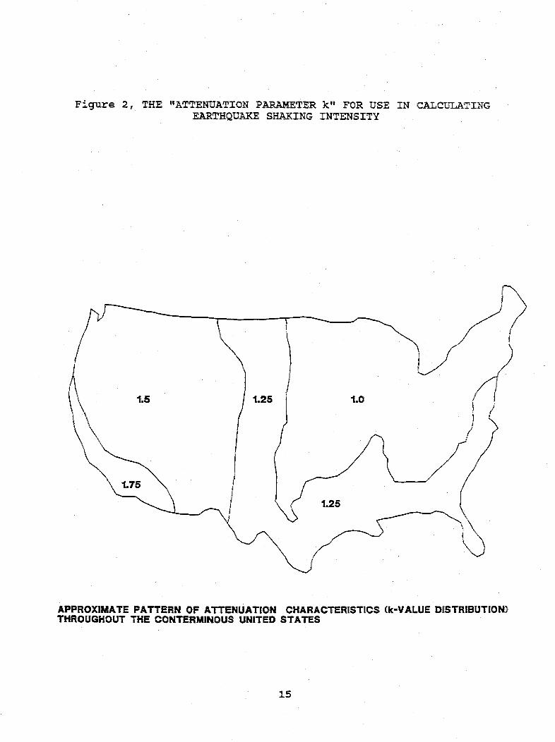
Figure 2, THE "ATTENUATION PARAMETER k" FOR USEEARTHQUAKE SHAKING INTENSITY
IN CALCULATING
APPROXIMATE PATTERN OF ATTENUATION CHARACTERISTICS (k-VALUE DISTRIBUTION)THROUGHOUT THE CONTERMINOUS UNITED STATES
15

ditigitized files of the U.S. Geological Survey topographic maps.Those maps include the routes of many of the lifelines and thegeographic elevation contours. Later when ground slopes are neededto calculate landslide and liquefaction potential, the computerprogram can be used to automatically perform the calculations.Thus, a single program can conveniently incorporate and graphicallypresent all the key data: lifeline location, fault traces, MMIvalues, and ground slopes.
Selection of the Earthquake Event
The next step is to identify the earthquake event for the analysis.Based on the faults in or near the study region, the QUAK2NW3program can be used to perform a sensitivity evaluation to identifythe appropriate earthquake event. All that is required is to inputvarious earthquake events (length and location of the faultmovement, the ground conditions, the depth of the earthquake, andthe attenuation parameter). The results of several analyses canthen be compared to identify the most realistic event for theanalysis. Key additional data that should be considered is theprediction of the magnitude and the probability that an earthquakewill occur near or in the study region. Such predictions areavailable from Federal and state seismologic offices.
4.2 Calculation of Lifeline Vulnerability-
Again, it is recommended that the lifeline owners/operators beconsulted to determine if they already have detailed calculationson their lifeline's vulnerability to earthquake events. If so,that approach may be the most detailed available. As analternative, the following sections identify how the ATC-13information, with important modifications, should specifically beused if such owner/operator information is not available.
Damage Assessment
To determine the potential damage state that occurs, the impacts ofshaking, fault displacement, and soil movement due to eitherlandslide or liquefaction conditions have to be considered. Thetotal damage state is the sum of these individual components;however, if one of these components dominates the others it can beused without adding the other damage states (this is often theactual situation). However, when that is done a similar approachmust be used for both the analysis performed while assuming nocollocation impacts and for the analysis performed while assumingcollocation impacts. Also, adding the separate damage states mayover estimate the total damage state. Knowledge of the physicalsituation and professional judgement must be applied to determinethe realistic total damage state.
There are seven categories of damage state defined in ATC-13. Theyare shown in Table 2.
16

Table 2ATC-13 DEFINITION OF LIFELINE DAMAGE STATE
Lifeline For Non Pipeline For PipelineDamage State Lifelines LifelinesNo. Description % Damage Breaks/kilometer % Damage1 - None 0 0 02 - Slight 0.5 0.25 0.63 - Light 5 0.75 24 - Moderate 20 5.5 145 - Heavy 45 15 3.86 - Major 80 30 757 - Destroyed 100 40 100
In the present method, the important parameter is theidentification of the Damage State Number, a number from 1 to 7.Thus, percent damage or breaks per kilometer are not the neededvariable. The experts that developed ATC-13 used the followingdefinitions for damage state: percent damage meant the estimate ofthe dollar value of the earthquake damage divided by the dollarcost to replace the entire lifeline. However, for pipelines theywere asked to think in terms of breaks in a pipeline per kilometerof pipeline length. Within a kilometer segment, 15 breaks mayactually cost the same as 40, since the expected procedure would beto simply replace the entire kilometer length rather than to makesuch a large number of individual repairs and still be concernedthat an additional partial break was undiscovered and thus remainedunrepaired. Similarly, an electrical transmission tower with 45%physical damage would probably be replaced entirely, as it wouldnot be worth the risk to the owner to make such extensive repairswhen a new tower may be less expensive to install and certainlywould be more reliable in the future. Thus, when the ATC-13definition is applied to a large number of similar lifelinecomponents, then, on the average, the damage state may properlypredict the condition of the sum of the individual repair costsdivided by the total replacement costs for all the components.
However, in the present analysis method, the ATC-13 data will beapplied to individual lifeline components. It is acceptable to usethe data in this. manner as it provides an expert knowledge base forestimating the damage state, and the final result of interest inthe present analysis method is not the damage state but a time torestore lifeline service. Its use for single lifeline componentswould be less accurate if the desired result were the percentdamage to be used to calculate a cost of repair (that is, ATC-13 ismore accurate for costs averaged over a large number of cases thanit would be for a single case). The proposed analysis methodcould, however, be improved if -a new expert opinion study of thedamage state and probability for that damage state for singlelifeline components were to become available.
The following material indicates how the data of ATC-13 are
17

proposed for use in evaluating the collocation impacts of lifelinesduring earthquake events.
Shaking Damage
The shaking impact of the earthquake event can be estimated byusing Table 7.10 (pages 198-217) of ATC-13. For convenience, themore frequently needed tables for lifeline analysis are reproducedin this report as Table 3.
These tables present the collective judgement of the probabilitythat a class of lifeline components will incur a given damage statelevel, as a function of the Modified Mercalli Intensity (MMI)index. They were developed by using a modified Delphi method thatemployed a large number of experts who provided their opinion as towhat was the probability that a damage level would be experiencedfor a given imposed value of shaking intensity, MMI.
The trend in the probability data would normally be expected toshow that, as the MMI increases, more of the lifeline componentswould be expected to experience higher damage states. Thus, forincreasing values of MMI, the shape of the probability curve shouldbe expected to have its peak value move towards higher damagestates and the magnitude of the peak value decrease as the width ofthe probability curve increases. However, at MMI = XII theprobability curve should again focus over the narrow band of damagestates 6 and 7. The information for bridges, highways, and buriedpipelines and conduits follow this pattern. It is less evident forelectrical transmission towers and railroads. The methodology forcalculating shaking damage collocation impacts, because it is basedon the ATC-13 data, will be less accurate for electricaltransmission towers and railroads, compared to buried pipeline andconduits, highways, and bridges. Still, the PrincipalInvestigators and Advisors for this project judged that the datawas adequate for the analysis purposes proposed in this report.
In Table 3 the lifeline items are: Facility Class 24-multiplesingle span bridges; Facility Class 25-continuous/monolithicbridges; Facility Class 31-underground pipelines; Facility Class47-railroads; Facility Class 48-highways; Facility Class 55-electrical towers less than 100 feet high; and Facility Class 56-electrical towers more than 100 feet high.
In this report the ATC-13 shaking damage data is used in thefollowing manner. For the lifeline component or segment beingconsidered, the appropriate table is entered using the MMI value atthe collocation'being analyzed. The table is entered to identifythe greatest probability value in the column under the MMI listing.In the sample below enter the table (on page 21) for MMI = VIII.Reading to the left of that maximum probability, the most probabledamage state is then read from the left most column.
18

Table 3SHAKING DAMAGE PROBABILITY MATRICES, ATC-13 Tables 7.10
Damage Probability Matrices Based on Expert Opinion forEarthquake Engineering Facility Classes
DamageState
Modified Mereaili IntensityMultiple Single Span Bridges
vYI VIi I III [S II XIII
1 3.0 iii fit Itt iii nj it
2 57.0 12.3 in i} in IF tiF3 i1i 85.7 70., fi t ri ii iti4 - fi i 29.1 71.1 iffi iM5 it Mi i 28.9 82.4 *ti t ii
6 iiit t1i i-n 1H.9 100.0 int7 i i ii off ii t 100.0
Continuous/Monolithic Bridges
v] V II VIII II I II III
1 93.6 8. 1 0.9 i ii itn ii2 6.4 77.8 17.6 itt it ii tt3 it 14.1 78.6 56.5 it i ifn
4 tit tt 2.9 43.5 1.9 1.2 0.75 i.E.! ii iii it 98.2 36.8 5.7
6 fiti i tit fit in 61.9 39.17 ti iii iti tit tin 0.1 54.5
lUnderground Pipelines and Conduits
VI VII VIII II I II XII
1 100.0 9.a, 20.9 8.7 tlIt ti it:2 it 0. 2 54.1 34.2 1.3 tit tlit3 itn a:: 17.2 36.1 7.9 os5 i1t4 it: t11 7.8 21.9 ;89.5 64.5 4.55 tit tit t1t 2t1 1.1 29.6 56.46 Itt tit t1t it: 0.2 3.3 37.97 ilI sit iI in Iti 0.1 1.2
***Very small probability
19

Table 3 (Continued)SHAKING DAMAGE PROBABILITY MATRICES, ATC-13 Tables 7.10
Modified Mercalli Intensity
Railr
VI ViI Vill
9.855.434.9
oft,
it#
0.112.387.00.6offoffit
-oads -
II I I1 III
M
0.373.925.8
off"I
',0
35.564.10.4off
MI
fit
10.280.89.0Hit
I..
III
tI
0.425.567.96.2tt
VI Yll
Highways
Vill ll
3.36.7
ftt
It
HIII
18.961.519.7tt
ftIII
2.927.068.8
1.4ittoffIII
Electrical Towers
VI VIl Vlll
94.15.9fittt
MHt
itt
6.978.814.3Ittott
.i.f
1.051.048.0itItt
HtIMI
Electrical Towers
VI VII Vll
93.66.4off
off
fit
it
itI
7.372.120.6
ttt
off
tII
itt
1.850.947.3
off
HfiII
Mt
1.0-13.875.49.8
Ht
Less
II
#iI
2.996.3
0.8If
*I
#it
it
1.359.039.10.6H
lt
Than 100 Feet High
I
63.736.3
MI
fiI
MI
More Than 100
1X I
III
7.592.20.3III
It*
it
oft
0.372.527.2iIIfitft
II Ill
itI
10.682.76.7itI
Feet
11
Ftt
16.679.44.0H
it§
***Very small probability
DamageState
1234567
94.15.9III
H,
tttHI Ht
1234567
I II XII
ilI
0.120.565.214.2
ft
itI
4.650.243.4
1.8off
1234567
1234567
III
0.539.059.21.3
High
Ill
III
0.838.25B.82.2i.
20

Sample ATC-13 Shaking Damage Matrix
Damage State Modified Mercalli Intensity IndexVI VII VIII IX X XI XII
1 100 99.8 20.9 8.7 - - -
2 - .2 54.1 34.7 1.3 - -
3 - - 17.2 36.1 7.9 .5 -4 - - 7.8 21.9 89.5 66.5 4.55 - - - - 1.1 29.6 56.46 - - - - .2 3.3 37.97 - - - - - .1 1.2
For a EMI = VIII, the largest probability is 54.1 (identified inbold); therefore the assumed damage state is damage state 2 (alsoin bold). The probability that the damage state or greater willoccur is the sum of its probability and all the probabilities forlarger damage at the MMI value of interest: (54.1 + 17.2 + 7.8) =
79.1%, or 79% for use in the subsequent analyses.
The data represented in Table 3 was developed based on assuming thefacility construction methods were in California. Since Californiahas incorporated seismic design criteria in some of their codes andstandards, it raises a question as to how the data should beapplied to other U.S. regions. The most direct approach would beto consider the design and construction practices at the study areain question, and to adjust the damage state predicted by Table 3 toaccount for differences with respect to California.
Rojahn 2 03 has developed a different approach. He suggests that theEMI value can be adjusted to account for the different design andconstruction practices. Increasing the MMI value would imply thatthe local practices are less conservative for earthquakeconsiderations than those used in California. Decreasing the XMIvalue would imply the opposite. Figure 3 shows the U.S. dividedinto seismic hazard regions. The Rojahn adjustments for arepresented in Table 4. He has used Figure 3 to divide the U.S. intofive broad regions: California region 7; Other U.S. areas, of region7; California regions 3 to 6; Puget Sound region 5; and all otherU.S. regions.
Table 4 is provided for information purposes. Data for additionallifeline components are provided in reference 20. Rojahn did notjustify the selection of the Table 4 values or explain whyadjustments are needed for California (recall that ATC-13 was basedon assuming that it applied to California). One of the importantrecommended follow-on studies to the present work is to apply thepresent screening tool to another U.S. location. One purpose ofsuch a study would be to examine the validity of the adjustments toMMI recommended by Rojahn.
21

Figure 3, MAP OF U.S. SEISMIC HAZARD REGIONS
NEHRP Seismic Map Areas OTC, 1978; BSSC, 1988).
Seismic RiskRegions
6 71 6
g S4
3
2
U1
22

Table 4EMI ADJUSTMENT FOR SHAKING DAMAGE EVALUATION
TO ACCOUNT FOR LOCAL CONDITIONS(the region numbers correspond to the numbers of Figure 3)
RegionCalifornia, #7Other area, #7California, #3-6Puget Sound, #5Other U.S. regions
Multiple Span Continuous Rail beds &Bridges Bridges Hichways
0 0 0I103
111
2 or 3
0000
Region and NumberCalifornia, #7Other area, #7California, #3-6Puget Sound, #5Other U.S. regions
RailroadBridges
-10
-101
Water Trunk Water PipeLines Distribution
O 10 10 10 11 2
Region and NumberCalifornia, #7Other area, #7California, #3-6Puget Sound, #5Other U.S. regions
Region and NumberCalifornia, #7Other area, #7California, #3-6Puget Sound, #5Other U.S. regions
Electrical ElectricalTowers Over Towers Less than100 ft. high 100 ft. high
0 'o 0
o 0Of 0
'0 1
Natural Gas Natural Gas OilTransmission Distribution Pipelines
-1 '0 -1-l-l-1
0011
-1-1-1-1
Fault Displacement
In ATC-13, the maximum fault surface displacement, D, in meters iscalculated from the equation:
Log D = -4.865 + 0.1719 x M; where M is the earthquakemagnitude
ATC-13 identifies that the fault average displacement is typically77% of the maximum, and that 30% of the maximum displacement on themain fault is characteristic of the displacement on subsidiaryfaults.
The damage states for the estimated displacement are obtained from
23

ATC-13 Table 8.9 and are presented in Table 5.
Table 5LIFELINE DAMAGE STATE FOR FAULT SURFACE DISPLACEMENTS,
ATC-13 Table 8.9
Facility Type Damage State (% damage is given in the parentheses)and Location For Various Values of Displacement in meters
Displacement = 0.2 m 0.6 m 1 m 3.5 m 10 mSubsurface StructureIn Fault Zone 5(50) 6(80) 7(100) 7(100) 7(100)In Drag Zone 4(20) 5(40) 5(60) 6(80) 7(100)
Surface StructuresIn Fault Zone 3(10) 4(30) 6(70) 7(100) 7(100)In Drag Zone 0(0) 0(°) 3(2) 3(10) 4(20)
The "Fault Zone" is defined as being within 100 meters of the faulttrace, the "Drag Zone" is defined as being within 100 to 200 metersof the fault trace. If lifeline components are judged to havefailed because of fault displacement, then the collocation impactwould be only an increase in the time to restore the lifeline toits needed level of operation (e.g., damage greater thancatastrophic is not meaningful). Such time increases would beattributed to the construction activity and the need to assure thatconstruction on one lifeline does not lead to damage onreconstructed other lifelines.
Soil Movement
Many texts separately define the impacts due to landslides andlateral spread (or liquefaction). However, they may be thought ofas being part of a continuum of soil movement with the slope of thetopography being a parameter that identifies whether the movementshould be calculated as a landslide or a lateral spread (orliquefaction). That is the approach proposed in the presentanalysis method.
Landslide (landslides occur on slopes greaterthan 50)
It is proposed that the historical landslides in the study area beidentified and considered as potential landslide req ions when thecollocation evaluation is made. Keefer and Wilsonsi0) and Sadlerand Morton" 1 ') have identified that landslides are associated withmany historical earthquakes and that shaking is one of the maintriggering agents for landslides. Actual site reconnaissancevisits are recommended as a means to verify the location ofhistorical landslides for any area being studied. In the presentstudy, a comparison of the known slides with the geologic unit mapidentified that many of the landslides were associated with areas
24

where Pelona Schist is the bedrock unit. Other researchers areadvised to examine the geologic sediments and rocks in the areaswhere they intend to evaluate collocation and to be sensitive tothe location of Pelona Schist.
It is proposed that the method of Legg et. al. CY2 ) be used toidentify additional areas where landslides may occur. It is basedon the sliding block model proposed by Newmark 1 3 ); Wilson &
Keeferc'4) have proposed a similar model.. However, the Wilson andReefer model requires using recorded accelerograms or predictionsof ground acceleration while the Legg method is related to usingMMI. The Legg model is the method used in ATC-13 to define thedamage state and probability of damage for landslides. Also, itwill be easier to apply the Legg model to other regions in theU.S.. Because of these items, the Legg method was adopted forpredicting additional landslide areas.
The Legg method consists of the following basic steps:
Step I Solve for the "critical acceleration" of the slopefor a given combination of slope angle and soilproperties. A formula derived from the stabilitysolution of an infinite slope was used by Legg andalso by Wilson and Reefer, and it is provided below.
Step 2 Use the critical acceleration to enter a table of"slope failure state"' versus DMI value. The tablevalues identify the potential for the slope to moveas a landslide. The tables are provided as Table8.7 of ATC-13 and are reproduced below as Table 7.
Step 3 The slope state is related to damage state in Table8.8 of ATC-13, which is presented below as Table 8.However, the ATC-13 Table 8.8 has been extended tomore accurately account for buried lifelines, basedupon expert opinion obtained during the presentstudy.
The formula for the critical acceleration is given by:
ar/g = c/(yh) + cos e tan ¢ - sin 0 ; where
a= the critical acceleration, ft/sec2
g = the gravitational constant, 32.2 ft/sec2
c = the effective soil cohesion factor, lb/ft2
= the soil density, typically 100 lb/ft3
h = the thickness of the soil block, typically 10 ftl = the slope angle, degrees
= the angle of friction of the slope material,degrees
Note, this equation applies to dry slopes.
25
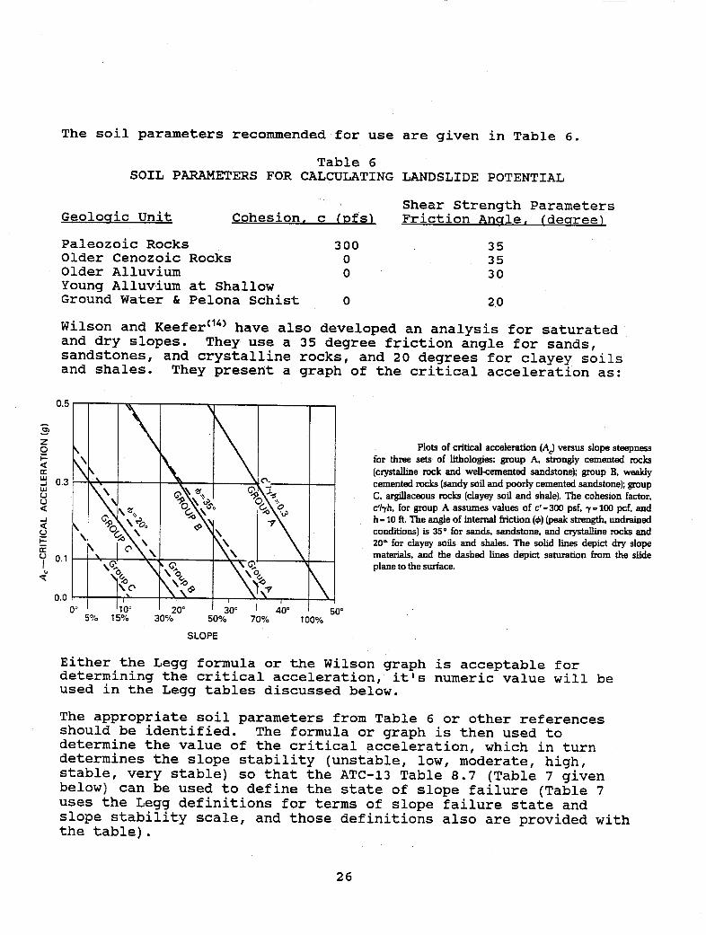
The soil parameters recommended for use are given in Table 6.
Table 6SOIL PARAMETERS FOR CALCULATING LANDSLIDE POTENTIAL
Shear Strength ParametersGeologic Unit Cohesion. c (Vfs) Friction Angle, (degree)
Paleozoic Rocks 300 35Older Cenozoic Rocks 0 35Older Alluvium 0 30Young Alluvium at ShallowGround Water & Pelona Schist 0 20
Wilson and Keefer (14 have also developed an analysis for saturatedand dry slopes. They use a 35 degree friction angle for sands,sandstones, and crystalline rocks, and 20 degrees for clayey soilsand shales. They present a graph of the critical acceleration as:
0.5 - -_ _ _ _ _ _ _ _
Z Plots of critical acceleration (Ad) versus slope steepness0
for three sets of lithologies: group A, strongly cemented rocksG% \ \ \ \(crystalline rock and well-cemented sandstone); group B, weakly
uj 0.3 ) v \ \ X \ cscemented rocks (sandy soil and poorly cemented sandstone); groupU \ \ O~y&> 9 96\ C, argillaceous rocks (clayey soil and shale). The cohesion factor,< 0 S C- 0 c'I'yh, for group A assumes values of c'-=300 psf. -y = 100 pcf. andX God O'er \S\ h -10ft. The angle of internal friction (e ) (peak strength, undrainedU \ '0< ,\ \ O \ 0 conditions) is 35° for sands, sandstone, and crystalline rocks and
I \\ \ 200 for clayey soils and shales. The solid lines depict dry slope_0_1 | materials, and the dashed lines depict saturation from the slide
plane to the surface.
10¢ 20' 300 i 400 5005% 15% 30% 50% 70% 100%
SLOPE
Either the Legg formula or the Wilson graph is acceptable fordetermining the critical acceleration, it's numeric value will beused in the Legg tables discussed below.
The appropriate soil parameters from Table 6 or other referencesshould be identified. The formula or graph is then used todetermine the value of the critical acceleration, which in turndetermines the slope stability (unstable, low, moderate, high,stable, very stable) so that the ATC-13 Table 8.7 (Table 7 givenbelow) can be used to define the state of slope failure (Table 7uses the Legg definitions for terms of slope failure state andslope stability scale, and those definitions also are provided withthe table).
26
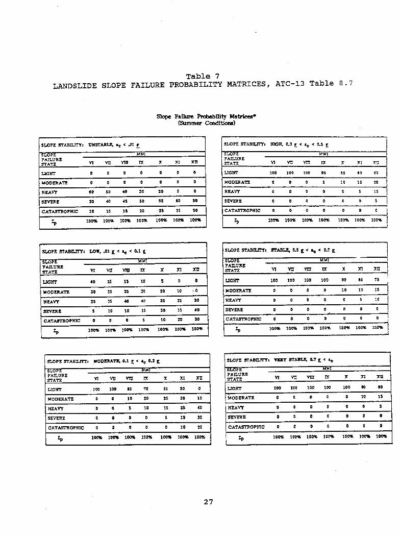
Table 7
LANDSLIDE SLOPE FAILURE PROBABILITY MATRICES, ATC-13 Table 8.7
Sope Fitflue Probabfity ¶abieft(Summer Conditico)
SLOPE SrABIErrY: UNSTABLE, .4 c .01 r
SLOPE YMIFAILURESTATE VI VD vm TX x Xl Xly
LUG&T 0 0 0 a 0 0 0
MODERATE a 0 a a a 0 0
HEAVY f00 50 40 30 20 5 a
SEVERI S0 40 45 50 55 60 S5
CATASTROPHIC l 1a i5 20 i5 15 50
½ 10I% 100% 100% 30% 100% 100% 2100%
LOnPE SriBLMrs LOW, .01 a , 0 c
SLOPE MMIYADLUR!STATE VI Vy Y3 ix X XI XE
LIGHT 40 25 15 10 5 0 0
iODERAIE 50 30 35 l0 20 10 0 O
HEAVY 25 35 40 40 35 35 30
SEVERC 5 10 10 15 20 35 40
CATASTROPHIC 0 0 a 5 10 20 30
½ 1 t00 100% 300% I00% 100% 100% 100%
SLOPE STABSLTYi XODIXATE, 0.1 a, -3 E
SLOPE MMIFhALURESTATE VI VI VM TX x xi
LIGHT 100 100 15 1 55 20 0
MODERATE O a 10 20 25 Jo 10
HEAVY 0 0 5 la 15 25 40
SEVERE 0 0 0 0 5 i5 20
CATASTROPHIC a a 0 0 0 10 10
Zp 100% l10 100% 100% 100% 300% l0
SLOPE STABEJrYza MIR, 0.3 p < a, c 0.5 r
SLOPEFAILUR ESTATE Vi VE vm rX X xi xEl
LIGHT 100 100 100 95 &5 !0 s0
MODERATE 0 0D 0 5 II 15 20
HEAVY 0 0 0 0 5 5 15
SEVERE C, o 0 0
CATASTROPH 0 a o0 0 0 0 0
Zp 100% 300%. 10a 100% 100% 1005S 10%
SLOPE SABUI STAEL., 0.5 c %( 0.7
SLOZ MMRFAGERFAILURESTATE VI vu vY 1x x X1 XII
LIGHT 10O 100 100 100 00 Is 75
MODERATE 0 0 0 0 10 l0 15
HEAVY 0 0 0 0 C 5 la0
SEVERE 0 0 0 0 0 0 C
CATASTROPHIC C 0 0 0 0 0 0
: D100%. 10096 I00 I00% 100% 100% 10C%
SIAPE sTABIlfrft Y=V 1TA l 0.1 E < 4e
SLOPE MMI
STATE V yn a TX X n XE
LIGHT 100 100 100 100 100 t SO
iAODERATE 0 0 0 0 0 1 15
HEAVY I 0 0 0 0 0 5
SEVERE 0 0 0 0 0 0 1
CATASTROPHIC 0 0 0 0 0 a 0
, 100 100 10100 %00% 100% 100% 100%
27
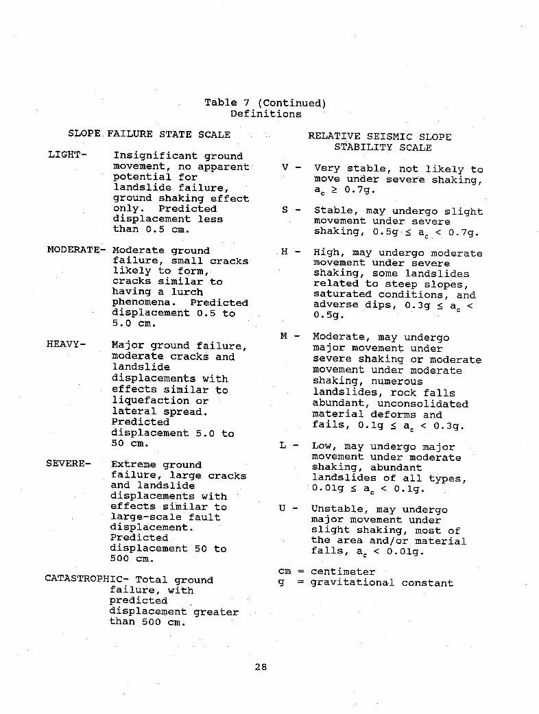
Table 7 (Continued)Definitions
SLOPE FAILURE STATE SCALE
LIGHT- Insignificant groundmovement, no apparentpotential forlandslide failure,ground shaking effectonly. Predicteddisplacement lessthan 0.5 cm.
MODERATE- Moderate groundfailure, small crackslikely to form,cracks similar tohaving a lurchphenomena. Predicteddisplacement 0.5 to5.0 cm.
HEAVY- Major ground failure,moderate cracks andlandslidedisplacements witheffects similar toliquefaction orlateral spread.Predicteddisplacement 5.0 to50 cm.
SEVERE- Extreme groundfailure, large cracksand landslidedisplacements witheffects similar tolarge-scale faultdisplacement.Predicteddisplacement 50 to500 cm.
RELATIVE SEISMIC SLOPESTABILITY SCALE
V - Very stable, not likely tomove under severe shaking,ac 2 0.7g.
S - Stable, may undergo slightmovement under severeshaking, 0.5g < a < 0.7g.
H - High, may undergo moderatemovement under severeshaking, some landslidesrelated to steep slopes,saturated conditions, andadverse dips, 0.3g < ac <0.5g.
M - Moderate, may undergomajor movement undersevere shaking or moderatemovement under moderateshaking, numerouslandslides, rock fallsabundant, unconsolidatedmaterial deforms andfails, 0.lg < ac < 0.3g.
L - Low, may undergo majormovement under moderateshaking, abundantlandslides of all types,0.0lg 5 ac < 0.1g.
U - Unstable, may undergomajor movement underslight shaking, most ofthe area and/or materialfalls, ac < 0.01g.
cm = centimeterCATASTROPHIC- Total ground g = gravitational constant
failure, withpredicteddisplacement greater :than 500 cm.
28

To use Table 7, it is necessary to enter it with the criticalacceleration, ac, and the MMI value. The critical accelerationvalue determines which sub-table is used. Within that sub-table,in the MMI column, identify the location with the peak probability.The slope failure state is read from the left-most column at therow that contains the peak probability value. The probability thatthe condition or worse will exist is the sum of the individualprobabilities for that slope state and all worse slope stateconditions. This is similar to how the shaking damage state andits probability were calculated.
Next, the slope failure status (light, moderate, heavy, severe,catastrophic) is converted to a damage state (and also a percentdamage) by using ATC-13 Table 8.8 (Table 8 below). ATC-13 providesa single conversion value for all lifelines.. This has beenexpanded in Table 8 to account for key buried lifelines. The newvalues were based on expert opinion obtained during the presentstudy.
Table 8CONVERSION OF LANDSLIDE SLOPE FAILURE STATE TO DAMAGE STATE
Damage State and (% Damage)
ATC-13 Values New Values Determine During This StudySlope Failure for all High Strength Low Strength
State Lifelines Lifelines Lifelines
Light 0-3 (0%) 0-2 (0%) 0-3 (0%)Moderate 4 (15%) 3 (0%) 4 (30%)Heavy 5 (50%) 4 (15%) 5 (60%)Severe 6 (80%) 5 (50%) 6 (90S%)Catastrophic 7 (100%) 7 (100%) 7 (100%)
The definition of high strength buried lifelines used to determinethe damage state is: continuous steel pipelines constructedaccording to modern quality control standards with full penetrationgirth welds; welds and inspection performed according to API 1104or equivalent.
The definition of the buried lifelines which should be representedby the original ATC-13 definitions is: pipelines and conduitsconstructed according to modern standards with average to goodworkmanship, other than the high strength lifelines defined above.Lifelines in this category are expected to include electric cables,steel pipelines with welded slip joints, ductile iron pipelines,telecommunication conduits, reinforced concrete pipe includingconcrete steel cylinder pipe, and plastic pipelines and conduits.Also, if the high strength lifelines are oriented so that thelandslide motion is expected to place them into compression, theyshould be analyzed in this category. Other lifelines not includedin the High Strength or Low Strength definitions should be
29

evaluated using the ATC-13 column.
The definition of low strength buried lifelines is: pipelines andconduits sensitive to ground deformation because of age, brittlematerials, corrosion, and potentially weak and defective welds.Lifelines in this category include cast iron, rivetted steel,asbestos cement, and unreinforced concrete pipelines; pipelineswith oxyacetylene welds; and pipelines and conduits with corrosionproblems. If other non high strength buried lifelines are orientedso that they are perpendicular to the expected landslide motion(e.g., their orientation is such that they will be put intocompression by the landslide), then they should be analyzed as alow strength lifeline rather than with the ATC-13 column.
Liquefaction or Lateral Spread (lateral spreadoccurs on slopes of 1-5°)
It is proposed that the Liquefaction Severity Index (LSI) be usedto correlate the liquefaction or lateral spread damage and theprobability of damage. The LSI is defined in the work of Youd andPerkins'15). The following material was developed from expertconsultive support provided during this study by Dr. T.D. O'Rourkeof Cornell Universityt 6 '8 '9 '1 6 '.
In a manner similar to the critical acceleration defined forlandslides, a critical LSI is defined in Table 9 below. The basisfor its use and the LSI damage probabilities of Table 10 is thework of Harding 6) which has shown that substantial lateralspreading can be triggered at a critical acceleration, ac, of 0.05to 0.15 g.
Table 9RELATIONSHIP BETWEEN LIQUEFACTION SEVERITY INDEX (LSI)
AND DAMAGE STATE
Physical Lateral EquivalentGround Movement LSI Damaqe State DamaQe Condition
< 0.5 inch <1 3 light0.5 to 5.0 inches 1-5 4 moderate5 to 30 inches 5-30 5 heavy30 to 90 inches 30-90 6 severe
> 90 inches > 90 7 catastrophic
O'Rourke has prepared a regression analysis of the observedrelationship between the MMI index and the LSI index for fourearthquakes; the 1906 San Francisco, the 1964 Alaska, the 1971 SanFernando, and the 1979 Imperial Valley earthquakes. Theobservations identified LSI values of 5 to 100 for MMI values of Vto X. The resulting regression curve (with an r2 = 0.68) is:
LSI=O . 226x1 0 0 255 x'MM
30
The equation can be used to calculate the LSI number, and thenTable 9 can be used to define the damage state. Graphically, therelationship between MMI and damage state is presented in Figure 4below.
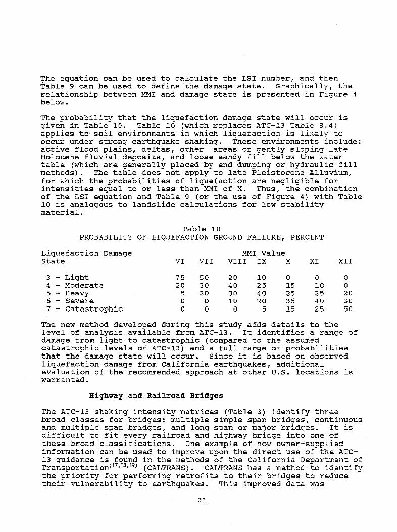
The probability that the liquefaction damage state will occur isgiven in Table 10. Table 10 (which replaces ATC-13 Table 8.4)applies to soil environments in which liquefaction is likely tooccur under strong earthquake shaking. These environments include:active flood plains, deltas, other areas of gently sloping lateHolocene fluvial deposits, and loose sandy fill below the watertable (which are generally placed by end dumping or hydraulic fillmethods). The table does not apply to late Pleistocene Alluvium,for which the probabilities of liquefaction are negligible forintensities equal to or less than MMI of X. Thus, the combinationof the LSI equation and Table 9 (or the use of Figure 4) with Table10 is analogous to landslide calculations for low stabilitymaterial.
Table 10PROBABILITY OF LIQUEFACTION GROUND FAILURE, PERCENT
Liquefaction Damage MMI ValueState VI VII VIII IX X XI XII
3 - Light 75 50 20 10 0 0 04 - Moderate 20 30 40 25 15 10 05 - Heavy 5 20 30 40, 25 25 206 - Severe 0 0 10 20 35 40 307 - Catastrophic 0 0 0 5 15 25 50
The new method developed during this study adds details to thelevel of analysis available from ATC-13. It identifies a range ofdamage from light to catastrophic (compared to the assumedcatastrophic levels of ATC-13) and a full range of probabilitiesthat the damage state will occur. Since it is based on observedliquefaction damage from California earthquakes, additionalevaluation of the recommended approach at other U.S. locations iswarranted.
Highway and Railroad Bridges
The ATC-13 shaking intensity matrices (Table 3) identify threebroad classes for bridges: multiple simple span bridges, continuousand multiple span bridges, -and long span or major bridges. It isdifficult to fit every railroad and highway bridge into one ofthese broad classifications. One example of how owner-suppliedinformation can be used to improve upon the direct use of the ATC-13 guidance is found in the methods of the California Department ofTransportation( 17 ,18 ,19 )' (CALTRANS). CALTRANS has a method to identifythe priority for performing retrofits, to their bridges to reducetheir vulnerability to earthquakes. This improved data was
31

LIQUEFACTION INDUCED DAMAGE7-
6
S~~
4--/ ,~~~~-0* Range Of Field Observation Data _
3- '-11
I ii III IV V VI VIl Vil IX: X Xi XIl
Modifed merCami index

integrated with the ATC-13 data to provide more discriminationcapabilities for evaluating railroad and highway bridges. Theresulting procedures (described below) are fully applicable tolocations outside of California if the needed data on theindividual bridges are known. The CALTRANS method includesfactors, such as traffic loading and detour routes1 that areimportant for making decisions about whether to spend money toretrofit a bridge, but they are not important for determining thedamage state of the bridge. However, other factors, such as thebridge sub and superstructure, the design codes used, and thebridge geometry can be related directly to the ability of thebridge to resist earthquake damage.
The method being proposed in this report calculates a parameterthat can be used to adjust the damage state value for shaking asdetermined by the ATC-13 matrices (Table 3 of this report). Theevaluation is based on starting with the ATC-13 shaking probabilitymatrix for Continuous and Multiple Span Bridges. The proceduresdiscussed above on how to use Table 3 to define the damage stateand the probability that the damage state or greater will occur areused to calculate a tentative damage state. A bridge vulnerabilityindex then is calculated and used to determine if the tentativedamage state should be changed (the probability is not changed).The decision to adjust the Table 3 tentative damage state value isbased on the numeric values identified below in Table 11 (highvalues of the Bridge Vulnerability Index mean that the damage willbe more severe than that predicted by Table 3).
Table 11RELATIONSHIP OF BRIDGE VULNERABILITY INDEX TO
BRIDGE DAMAGE STATE
Change to Table 3 ContinuousBridge Vulnerability & Multiple Span BridgeIndex Value Damaae State Value
0.0 - 0.2 Lower the Damage State bytwo increments
0.2 - 0.4 Lower the Damage State byone increment
0.4 - 0.6 No Change
0.6 - 0.8 Increase the Damage State byone increment
0.8 - 1.0 Increase the Damage State bytwo increments
33

The numeric value of the Bridge Vulnerability Index is calculatedby multiplying a Raw Score by a Multiplying Factor (in theCALTRANS' method, the terms were weighting factor and pre-weightingfactor, respectfully). The Raw Score is assigned by the importanceof the bridge factor being evaluated, the Multiplying Factor is aweighting scale that determines how earthquake resistant the RawScore items is. Table 12 presents the numeric values of the RawScore and the Multiplying Factors.
There are seven categories that are analyzed: 1) abutments; 2)piers; 3) soil type; 4) superstructure type; 5) design code orspecification used; 6) bridge height; and 7) bridge skew andcurvature. A separate number (the raw score times the multiplyingfactor) is calculated for each of the seven categories and then theindividual numbers are summed. The sum is divided by 100 to givethe total Bridge Vulnerability Index value.
In applying the incremental change to a tentative damage state fromTable 3, if this results in a damage state less than 1 or greaterthan 7 use those limit values. Damage states for long span (lengthgreater than 400 feet) and major bridges may be estimated usingthis procedure, but it is recommended that such structures besubjected to special studies whenever possible. It is emphasizedthat the above Bridge Vulnerability Index is for shaking damage.Special conditions, such as liquefaction, require additionalanalysis.
The analysis factors required to enter Table 12 can be obtainedfrom the general design drawings of the bridge or by fieldreconnaissance. Some assumptions may have to be made with respectto foundation design in the latter case.
Railway bridges have proved to be somewhat more resistant to groundshaking than highway bridges, in spite of the fact that theAmerican Railway Engineering Association (AREA) specifications makeno specific recommendations with regard to earthquake forces. Thisis probably due to the fact that railroad brides have an allowancefor lateral loads (originally, the allowance was to account for theloads produced by steam locomotives). Prior to 1935, thisallowance was 5% of the live load (typically based on a Cooper E60engine, or about 852,000 lbs. on a 109 ft. span), but not more than400 lbs. per foot of track. In 1935, this was changed to providefor a lateral load of 20,000 lbs. applied at the top of the rail atany point in the span. In 1950, AREA provided for higher allowablestresses, so that the allowance became somewhat less conservative.The multiplying factors of Table 12 for railroad bridges reflectsthese facts.
34

Table 12BRIDGE VULNERABILITY INDEX FOR EARTHQUAKE SHAKING DAMAGE
Multiplying Factor CriteriaMultiplyingFactor Value
SUBSTRUCTUREAbutments
Piers
10 Integral with pile foundationIntegral with spread footingHinge seat with restraintsHinge seat, all other types
15 wallmultiple column bentsingle column bent
0.00.50.61. 0
0.20.5
Note, if a spread footing foundation is used, add 0.2 to thepier multiplying factor, if the columns have been reinforcedto recent seismic codes, subtract 0.3 from the piermultiplying factor.
Soil Type
SUPERSTRUCTUREType
15 Rock or soil with bearing ofmore than 4 tons/ft2 0.0
Soil with bearing of 2 - 4 tons/f t 0.1Soil with bearing of less than 2 tons/ft2 0.5
20 Highway BridgesSimple span, box or slabSingle span, arches, reinforced concrete
*or well constructed masonrySimple span, steel or concrete beamsSimple span, steel trussMultiple spans, continuous with no hingesMultiple spans, continuous with 1 hingeMultiple spans, simple beamsMultiple spans, continuous with 2 or
or more hinges
ro . o
O0 . 1
0.50.50. 00.51. 0
1 . 0
Railroad BridgesSimple spans, steel with full trussSimple spans, deck or half trussSimple spans, steel or concrete ballastedSimple spans, steel or concrete beamsMultiple spans, fully continuousMultiple spans, simple beams.Multiple spans, continuous with hinges
0.30.40..51..00.01.01.0
Note, for both highway and railroad bridges with hinges,subtract 0.4 from the multiplying factor if restrainers havebeen added. Subtract an additional 0.3 if the columns havebeen reinforced to resist earthquake forces.
35
BridgeElement
RawScore

Table 12 (Continued)BRIDGE VULNERABILITY INDEX FOR EARTHQUAKE SHAKING DAMAGE
Bridge Raw MultiplyingElement Score Multiplying Factor Criteria Factor Value
DESIGN CODE OR SPECIFICATIONCode used 20 Highways
CALTRANS* after 1978 or AASHTO* after 1987 0.0CALTRANS between 1972 and 1978 0.2CALTRANS prior to 1972 andAASHTO prior to 1950 0.5AASHTO from 1950 to 1987 1.0
Note, AASHTO, from 1950 to 1987, leaves the earthquakeconsiderations to the States. If it is known that the State hasno such consideration, use 2.0 as the Multiplying Factor value.
RailroadsAREA* from 1935 to 1950 0.5AREA from 1950 to present 0.7AREA prior to 1935 0.8
Note, for the condition of bridge, modify the design code orspecification Multiplying Factor by adding the following to thefactor:
Good or fair condition 0.0Poor condition 0.2
GEOMETRYHeight 10 Less than 5 feet 0.2
5 to 15 feet 0.715 to 25 feet 0.925 feet and greater 1.0
Skew* and 10 Skew less than 200 andcurvature radius greater than 1000 ft. 0.0
Skew 200-400 and/orradius greater than 500 ft. 0.1
Skew greater than 400 and/orradius less than 500 feet 0.4
Key *AASHTO, American Association of State Highway & Transportation
OfficialsAREA, American Railroad Engineering AssociationCALTRANS, California Department of TransportationSkew is defined as the angle that abutments and piers make withrespect to the normal to the highway (or railway) alignment.That is, when the plane of the abutment or pier is alignedparallel to the normal to the road (or rail bed) alignment, theskew is 0°.
36

Times to Restore the Lifeline to its Needed Service
Once the lifeline components of interest have been identified andthe damage state and probability that the damage condition or worsewill occur have been calculated from the above tables and formulas,the time to restore the lifeline component or segment from thetotal calculated damage state to the operating level needed has tobe determined.
The restoration time is a combination of the time to repair the
lifeline segment or component assuming all the equipment, material,and personnel are available at the damage site, plus the accesstime to get the equipment and material to the damage site, plus thedelay time needed to obtain the equipment and material required for
making the repair. The way to calculate these items is given next.
Repair Time to restore the damaged lifeline to service
With the damage state known, the time to rep-air the lifelinecomponent or segment (assuming the equipment and material are atthe damage location) can be calculated from Table 9.11 of ATC-13.The key information of Table 9.11 is provided below as Table 13.If intermediate operating conditions (e.g., repair to less than100% capacity) are acceptable, the intermediate repair times of theATC-13 tables can be used or the plots of those tables provided byRojahn(20) can be used to estimate such intermediate conditionrepair times. The newer curves by Rojahn are curve fits of thedata of ATC-13l23, thus they are not exact replications of the data.But they may be more convenient to use since they relate the repairtime to MMI instead of to the damage state as is done in ATC-13.Also, if there is concern about the magnitude of the repair timeestimated, Table I.1 of Appendix I of ATC-13 can be used todetermine the range of repair times identified by the experts thatprepared Table 9.11. It is important to recognize that the actualrepair time is not used directly to estimate the impact ofcollocation on the vulnerability of lifelines to earthquakes (aswill be shown below).
Eleven of the more important repair tables are presented in Table13 (some of the tables were adjusted from the ATC-13 values toaccount for expert opinion obtained during the present study). Tomake a specific estimate of lifeline repair time, enter the properlifeline table at the row that identifies the damage state and moveto the right until the correct lifeline column is encountered.Then read the time, in days, required to restore the lifeline tofull capacity from that damage state. The ATC-13 lifelines ofinterest are: lac-petroleum transmission pipelines, 25a-highwaymajor bridges, 25c-highway conventional bridges, 25d-freeways andhighways, 26a-railroad bridges, 26c-railroad roadbeds, 29b-electrical transmission towers, 30f-water trunk lines, 31a-sewerlines, 32a-natural gas transmission lines, and 32d-natural gasdistribution lines. It should be recalled, however, that better
37

estimates of repair time are probably available from the individuallifeline owners, as they may have site specific conditions includedin their estimates.
.Table 13ESTIMATED LIFELINE REPAIR TIMES TO 100% OPERATING CAPACITY
ATC-13 Table 9.11(Times in Days)
RailroadBed**
112
114182
120
Highway**Conventional
Bridge118
84303686752
HighwayMajorBridge
127
141392845947
RailroadBridge
118
58213468606
Natural Gas** Natural GasDistribution & TransmissionPetroleum Lines Pipelines
1 1136
194455
13
11254475
FiberOptic**Conduits
1113
102430
ElectricalTransmission SewerTowers Lines
1 11 32 5
17 1849 6382 102
127 141
* Damage State 1 has a 1 day allowance to allow forinspection to determine the actual damage state thatexists at the lifeline
** These values were determined by expert opinion duringthis study
Access Time to get the equipment and material to thedamage site
Next it is necessary to estimate the time to get the equipment andrepair material to the site. This time is the time to getconstruction equipment and material to the damage site, and itshould not be confused with the time it would take to get generalpopulation traffic to the site or with the time it would take forrepair crews to get to the damage site. In many situations, andespecially for lifelines such as pipelines, fiber optics, andelectrical transmission towers, most of the necessary equipment andmaterial can be driven to the damage location either along thehighways, unpaved access roads, or cross country if the land is dry
38
DamageState
1*234567
HighwayBed
117
41147292437
WaterTrunkLine
123
102574
156
DamageState
1*234567

and accessible. In some of the more rugged regions they can behelicoptered to the site. An exception would be if wet ground orlarge water bodies must be negotiated. Thus, in general, for thoselifelines the access time is one or two days, depending upon thelocation of the segment or component of the lifeline system beingexamined. If access along the highway is required it should becalculated as described below for the railroads and the highways.
For many of the railroad or highway components and segments, theaccess will have to be along the railroad or highway itself becauseof the size and weight of the material and equipment that isrequired. In such cases, it will be necessary to estimate therepair times for damage along the route prior to the location beingstudied. The individual repair times must then be added for eachdisruption that occurs before the location being studied to obtaina total estimated access time. Alternatively, detours can be usedto calculate a "by pass" time estimate.
Equipment and Material Time to have those items available
For many of the lifelines, the owners have their own operatingequipment and have prepositioned repair material along theirlifeline routes. When they don't have suitable repair equipment intheir operating stock, they may have existing agreements with otherfirms, to provide such equipment during emergencies. Frequently,utility lifeline owners have reciprocal agreements with otherutilities to provide personnel and equipment during emergencyperiods. This preplanning can decrease the time it takes to haveequipment and repair material available to transport to the damagelocation.
The problem of material availability can be pronounced for railwayand highway bridge repairs. In those cases, the time required tofabricate off site the needed components must be accounted for inthe estimation of the delays in having equipment and materialavailable.
In almost all cases, it can be assumed that the equipment will notbe available during the emergency phase of the earthquake, since itwill be diverted to life-saving duty at that time. However, priorearthquake response experience indicates that most equipment andneeded material will be made available within one or two days.
4.3 Collocation Analysis
Section 4.2 presented a number of analysis methods that can be usedto determine the damage state, the probability that the damagestate or worse will occur, and the estimated restoration time toreturn each lifeline component or segment to its needed servicelevel.
In the collocation analysis activities, a collocation damage
39

scenario is developed and the unknown conditions (either damagestate, probability of damage, restoration time, or any combinationof those items) are recalculated for the assumed collocation damagescenario using the methods of Section 4.2. The collocation damagescenario should be based on the knowledge of how the individuallifelines would have responded if they had be the only lifeline atthe collocation point, the estimate of the types of impacts thatone lifeline failure could impose on another nearby lifeline, andthe zone of influence that one lifeline has.
This process requires that technical judgements be applied, basedon knowing the expected damage states of the collocated lifelines,the seismic and geologic conditions, information about thelifelines themselves (such information as the design conditions,construction history, repair and maintenance history, and otherpertinent facts), and other lessons learned from prior earthquakes.It will be important to obtain as much information from thelifeline owners as possible to help guide the collocation damagescenario analyses.
It is also important to recognize that there is a zone ofinfluence, beyond which the impact of one lifeline on another wouldbe negligible. During this study, expert opinion was used toestimate the appropriate radii of influence zones for the lifelinesfound in the Cajon Pass. The results are given in Table 14.
Care must be taken to differentiate between the zone of influenceand the actual influence or damage caused. For example, the zoneof influence of a failed dam is based on the path of the water thatspills past the dam. It includes the actual pathway and the areathat the water would inundate. The actual impact of the failed damcould be erosion of foundations of other lifelines (thereby causingthem to collapse) or the flooding of them (perhaps restrictingtheir ability to function). There may be no influence on onelifeline, while the impact on another could be pronounced. Some ofthe impacts may be subtle. For example, a failed communicationlifeline may have no immediate impact on the physical state orcondition of other nearby lifelines. Its impact, however, could betied to increasing the restoration time of nearby lifelines due tothe difficulty of maintaining communications with the repairpersonnel. In the present context of lifeline vulnerability, theimpact of one lifeline on a collocated or nearby lifeline can bethe damage state, the probability of damage, or the restoration ofservice time. Other impacts, although real, have no way to beaccounted for in the analysis method.
Although the values in Table 14 are considered appropriate for thesemi-desert region of the Cajon Pass, California, for which theywere prepared, it will be important to validate these values whenthe lifeline zones of influence are evaluated for other at-risk orcollocation conditions.
40

Table 14LIFELINE ZONES OF PHYSICAL INFLUENCE
Liquid Fuel Pipeline -
Natural Gas Pipeline -
Fiber Optic Cables -
Roadways -
Railroads -
Overhead Electrical -
Transmission Towers &Power Lines
Bridges -
Dams., Reservoirs & -
Canals,
Water & Sewer Lines -
The drainage path and catchment areafor any liquids spilled; two timesthe pipe burial depth for any soilcratering impacts due to pipelineruptures; 100 feet if explosionimpacts are estimated; ground erosionpaths for liquids spilled; and theburn path if fires are estimated.
Two times the burial depth for anysoil cratering impacts due topipeline ruptures.; 100 feet ifexplosion impacts are estimated; andthe burn path if fires are estimated.
Zero feet (e.g., no physical impacton other lifelines).
40 feet from the road edge; apossible ignition source for fuellifelines.
40 feet from the track edge; apossible ignition source for fuellifelines.
A radius equal to the height of thetower for physical contact;a possible source of ignition forfuel lifelines.
For an area centered on the bridge,twice the length of the bridge and 40feet-on either side of the bridge.
The drainage path and inundationareas for the spilled water.
The erosion area downstream of thebreak (sewers only if they arepressurized); the catchment area forthe spilled fluids.
It is anticipated/ but not required, that collocation impactscenarios will follow the following general guidance.
41
Impacts on Damage State
One of the easier direct impacts to hypothesize will be that thecollocation conditions will lead to an increase in the damage stateof one or both of the collocated lifelines (if there are more thantwo collocated lifelines this applies to all of them). It is easyto understand the damage state, as it relates to a physicalcondition. Because the individual lifeline damage states assumingno collocation are known, those values can be used to helpunderstand how the lifeline could impact another nearby lifeline.If, for example, light damage of a pipeline had been calculated, itwould be expected to cause no direct change in the damage state ofa nearby bridge. However, if the bridge had been estimated tocollapse, it would be reasonable to estimate that within thebridge's zone of influence it would lead to failure of the pipeline(this example also illustrates that the impacts are not necessarilyreciprocal).
As another example of how collocation impacts on damage state canbe estimated, consider the condition of a pipeline and a fiberoptic conduit hung from a bridge. The earthquake vibration may notbe enough to cause serious damage to the bridge or to the pipelineor conduit if they were not collocated with each other. However,the vibrations may cause the anchors holding the heavy pipeline tothe bridge to fail. As the pipeline sags (but does not fail) itcould fall onto the lower conduit, causing it to fail. Thecollocation damage state hypothesis would then be: no impact on thebridge; a small increase in damage state of the pipeline to accountfor the work required to rehang the pipeline; and catastrophicfailure of the fiber optic conduit.
Special attention should be given to the collocation of fuelcarrying lifelines with other lifelines that have the ability toprovide an ignition source. The resulting fire and/or explosioncould lead to significant collocation damage. Similarly, brokenpipelines which eject fluids could lead to foundation erosionproblems that would result in increased damage to nearby lifelines.
Impacts on Probability of Damage
The probability of damage does not directly enter into thecalculation of the damage state level or the time to repair thedamage. It is, as will be discussed below, a very important itemfor determining the key result of the collocation analysis, theprobable incremental change in restoration of service time.
There are several ways to estimate the change in the probabilitythat damage will occur, none are exact and there are no statisticsavailable from the literature on earthquakes. However, there aresome insights available to guide the analysts.
If the probabilities for two lifelines, assuming no collocation
42

conditions, are P1 and P2, they represent an upper bound on the
probability that a collocation damage would occur. For example, if
the probability that lifeline 1 would fail is PI, and it is, known
that if lifeline I fails it will cause, with -a 100% probability,
damage to lifeline 2, then the probability that lifeline 2 receives
collocation damage is also P1 (e.g., P1 x 100%). Similarly, the
upper bound on the probability that lifeline 2 has damaged lifeline
1 is P2.
As a practical matter, the collocation damage likely will be less,
since there is seldom a 100% chance that the collocation damage
scenario will occur. A useful measure of the probability that the
collocation event has occurred is the product of the two
probabilities that the single independent events that were used to
develop the collocation scenario have occurred (the independent
events are the estimate of the damage state of each lifeline
assuming there was no collocation). In the present case, that is
found by multiplying PI x P2. The product can be interpreted as
follows. It represents the increase in probability that the two
independent lifeline damages will occur during the same initiating
event. If both events must occur before the collocation damage
scenario can take place, then it is a measure of the probability of
the collocation damage scenario.
The actual probability that the collocation event will occur should
be a number between the numerical limits of P1 and (PI x P2) for
having lifeline 1 cause additional damage to lifeline 2, and P2 and
(P2 x Pi) for having lifeline 2 cause additional damage to lifeline
1. It is recommended that for calculational purposes, the product
Pi x P2 be used to characterize the hypothesized collocation damage
scenario.
Impacts on Time to Restore Lifeline Service
As discussed above, the time to restore lifeline service is
composed of the sum of the time to repair the lifeline damage, the
time to access the damage site with equipment and material, and the
time to obtain the equipment and material.
The hypothesized collocation damage scenario does not have to
assume a repair time. Once the collocation damage state is known,
the repair time can be obtained from Table 13.
However, it is reasonable to include in the collocation damage
scenario impacts on accessibility to the damage site, which has the
impact of increasing the overall restoration of service time
estimate. In fact, this is probably one of the more significant
aspects of the collocation damage scenario, e.g., the estimation of
the additional direct delays that will be incurred because of the
collocation of the lifelines. The greater the level of damage
estimated for each of the separate lifelines, assuming that there
is no collocation, the greater the anticipated delays that will
43

result from their actually being collocated.
The following are offered as possible examples of how collocationcould create access delays that would increase the time to restorethe lifeline to service. General congestion at the collocationlocation because there are multiple lifelines could delay the startof repair work on a lifeline. Concern over the possibility ofleaking fuel may cause all work to be delayed until it can beconfirmed that it is safe to have workers in the area. Spilledliquid fuels may have to be treated and/or removed beforeconstruction vehicles and welding (which could provide an ignitionsource for fuel vapors) would be allowed.
Work on a pipeline buried next to a railroad may be delayed whiledebris about and on the railroad is removed by heavy equipment.Then, because of the weight of the debris and/or the heavyequipment, the entire pipeline may have to be exposed and inspectedbefore it is allowed to return to service. Often, powertransmission towers are replaced with temporary towers while repairwork on the damaged tower is performed. However, the use of atemporary tower may limit the access of pipeline and transportationlifeline repair crews because of the increased potential forelectrocution if heavy equipment is operated near the temporarytower. Fires at collocation locations can increase the timerequired to inspect the nearby lifelines to determine the extent,if any, of damage caused by the fire. Water inundation can causedelays until the water is drained and the surrounding ground driesto a condition that allows the repair equipment and material to bedelivered to the damage site. Major damage to a lifeline mayresult in a regulatory review about the suitability of rebuilding(or repairing) the lifeline. While the regulatory review isunderway the repair on the lifeline may be delayed.
In summary, a collocation damage scenario must be developed, basedon the knowledge of the lifelines and their anticipated damagestate if they had been isolated or non-collocated. This willresult in the estimation of a new damage state, new access times,or combinations of those items. With the damage state known, a newrepair time is calculated, and the repair time and access time areused to determine the new time to restore service.
4.4 Interpretation of the Results
This is the activity that brings together all of the previousanalyses.
The most appropriate measure of the impact of lifeline collocationbecause of an earthquake was judged to be the most probableincremental increase in the time to restore the lifeline to itsneeded service level. The restoration of service time is a broadmeasure of the impact of lifeline damage on personnel, equipment,and material resources, it does not measure the impact that the
44

loss of the lifeline has on the community that was relying upon it.The difference between the restoration of service time assumingcollocation impacts and the shorter restoration time found byassuming no collocation impacts gives the incremental impact thatcollocation has caused to service restoration. The incrementaltime impact is a better measure of collocation impacts as comparedto the estimated total time to restore service, because any biasesin the estimation procedures tend to be canceled by the subtractionprocess.
It is important to multiply the incremental change in restorationtime by the probability that the collocation damage has occurred.This recognizes, the uncertainties in the data base and analysismethods provided in Section 4.2, and it also recognizes that inactual earthquakes there is a real probability that a given levelof damage will occur, or conversely, will not occur. The product,incremental change in restoration time multiplied by probability,identifies the most probable incremental change in restorationtime.
There are two ways to use the final measure:
1) the most probable incremental change in restoration timecan be considered at a specific collocation site to evaluatethe impacts at that site. This will provide an insight on thevulnerabilities that occur when specific types of lifelinesare collocated at at-risk locations. That is, this type ofinformation will help identify which lifeline types or whichlifeline design or construction practices, when collocatedwith other lifelines, lead to the greatest increases to theother lifelines' level of vulnerability.
2) the most probable incremental change in restoration timecan be summed along the route of a given lifeline to providean insight on the impacts that the specific lifeline route hashad on the vulnerability of the lifeline.. This type ofinformation can be used to help identify undesirable routingdecisions.
4.5 Chapter 4.0 Bibliography
1. P. Lowe, C. Scheffey, and P. Lam, uInventory of Lifelines inthe Cajon Pass, California", ITI FEMA CP 120190, August 1991.
2. C. Rojahn and R. Sharpe, "Earthquake Damage Evaluation Datafor California"l, ATC-13, 1985.
3. J. Evernden, et. al., "Interpretation of Seismic IntensityData"t, Bulletin of the Seismological Society of America, V 63,1973.
45

4. J. Evernden, et. al., "Seismic Intensities of Earthquakes ofConterminous United States - Their Predictions andInterpretations", U. S. Geological Survey Professional Paper1223, 1981.
5. S. Algermissen et. al., "Development of a Technique for theRapid Estimation of Earthquake Losses", U.S. Geological SurveyOpen File Report 78-441, 1978.
6. Harding Lawson Associates, et. al., "Marina District &Sullivan Marsh Area Liquefaction Study, San Francisco,California", Draft report prepared for the City & County ofSan Francisco, June 1991.
7. J. Davis, et. al., "Earthquake Planning Scenario for aMagnitude 8.3 Earthquake on the San Andreas Fault in SouthernCalifornia", California Division of Mines and Geology, SpecialPublication 60, 1982.
8. S. Barlett and T. Youd, "Case Histories of Lateral SpreadsCaused by the 1964 Alaska Earthquake", US/Japan Case Historiesof Liquefaction. Large Ground Deformation and Effects onLifeline Facilities, NCEER, in press.
9. T.D O'Rourke, et. al., "Large Ground Deformation and TheirEffects on Lifeline Facilities: 1906 San FranciscoEarthquake", US/Japan Case Histories of Liquefaction, LargeGround Deformation and Effects on Lifeline Facilities, NCEER,in press.
10. D. Keefer and R. Wilson, "Predicting Earthquake-InducedLandslides, with Emphasis on Arid and Semi-Arid Environments",Landslides in a Semi-Arid Environment with Emphasis on theInland Valleys of Southern California, Edited by P. Sadler andD. Morton, 1989.
11. P. Sadler and D. Morton, Editors, "Landslides in a Semi-AridEnvironment with Emphasis on the Inland Valleys of SouthernCalifornia", Publications of the Inland Geological Society,Volume 2, 1989.
12. M. Legg, M., J. Slosson, and R. Eguchi, "Seismic Hazard forLifeline Vulnerability Analyses", Proceedings of the ThirdInternational Conference on Microzonation, Seattle,Washington, 1982.
13. N. Newmark, "Effects of Earthquakes on Dams and Embankments",Geotechnique, v.15, No. 2, p. 139-160, 1965.
14. R. Wilson and D. Keefer, "Predicting Aerial Limits ofEarthquake Induced Landsliding", Evaluating Earthquake Hazardsin the Los Angeles Region, U.S. Geological Survey Professional
46

Paper 1360, 1985.
15. L. Youd and R. Perkins, "Mapping of Liquefaction SeverityIndex", Journal of Geotechnical Engineering, Vol. 113, No. 11,pp 1374-1392, 1987, and "Mapping Liquefaction Induced GroundFailure Potential", Journal of the Geotechnical EngineeringDivision, ASCE, 104, GT4, pp 433-446, 1978.
16. T.D O'Rourke, et. al., "Large Ground Deformation and TheirEffects on Lifeline Facilities: 1971 San Fernando Earthquake",US/Japan Case Histories of Liguefaction, Larae GroundDeformation and Effects on Lifeline Facilities, NCEER, inpress.
17. "Seismic Design Procedures and Specifications 1940 to 1968",CALTRANS Division of Structures, material provided for theCajon Pass Lifeline Study, September 1990.
18. B. Maroney and J. Gates, "Seismic Risk Identification &Prioritization in the CALTRANS Seismic Retrofit Program",material provided for the Cajon Pass Lifeline Study, September1990.
19. "1CALTRANS Seismic Risk Algorithm For Bridge Structures", SASADivision of Structures, June 30, 1990, material provided forthe Cajon Pass Lifeline Study, September 1990.
20. C. Rojahn, C. Scawthorn, and M. Khater, "Seismic Vulnerabilityof Lifelines in the Conterminous United State", ATC-25, inpress.
21. T. Airman, et. al., "Pilot Study on Seismic Vulnerability ofCrude Oil Transmission Systems", NCEER-90-0008, May 1990.
5.0 APPLICATION THE METHOD TO CAJON PASS
5.1 Data Acquisition
The following material demonstrates the application of the analysismethod described in Section 4.0. The first step of the process is,to assemble the data base that describes the lifelines and theirroutes in the study area as well as the geologic and seismicsituation. The earlier Cajon Pass studytl) provides most of theneeded information. It should be consulted for specifics abouteach lifeline and when it was installed.
Figure 5 shows the Cajon Pass study area and its relationship toother cities in California. It is used with the permission of theAutomobile Club of Southern California (it is copied from the SanBernardino County and Las Vegas Area map). It shows that the CajonPass canyon (which is about 10 miles northeast of San Bernardino)is a natural access route between the San Gabriel Mountains to the
47

Figure 5, MAP OF THE GENERAL LOCATION.OF THE CAJON PASS STUDY AREA
___ L E 1Y9 '
* I l,
inI
~ t* 0 ,..Study Area
WI ,^;* -n a. * = °h°pit. ,ftw.-
- 3LN Mtdsi. lul*_ l AM L
a IW AM 1FIAIX10 -r-
'LA VERNE~ M'~. CUAMONGA >..- - ABErARMk l . CLBO OTM AMP
PLAN -... NT ~~~~~~~~~IALI -'ACiBFA ** .,~~~~~~~~~~~ f'f~~~~~~~-lll'flb 19 - -C -!
.UN1AMU :;_
Si CHINO-
I _ -,.a. - - ,,la-!
o.- I6 .k4 -B ,
DEE'2~ ~ MORENOmIoRn ARaAM-.'-
1' A LA NhlA YILLAIE **.~- 8.,A4
-', - -
48
i-.
* ' .._ ^
-
0sl. _.._...~~ I^ C- q Nm
.s _ss-.*
'I 7:NP PMONA

west and the San Bernardino Mountains to the east. The Passconnects the Los Angles Basin in the south to the high desertregions to the north. The City of San Bernardino is about 10 milessoutheast of the mouth of the Pass.
U.S. Geological Survey quadrangle maps (7.5 minute seriestopographic maps published in 1988) were used to obtain more detailand to develop a plan for a site survey. The site survey was thenconducted. It identified additional lifelines that were notidentified on the 7.5 minute quadrangle maps, which emphasizes theheed to conduct actual site surveys to validate the publishedinformation on lifeline systems. With the map and site visitinformation as a background, the individual lifeline owners werecontacted and meetings were held with their staff to obtain moredetails on the location, capacity, design basis, operating andmaintenance history, and emergency response systems in place foreach lifeline. The Cajon Pass site was revisited to validate ourunderstanding of the actual siting conditions, and in some casesthis led to additional visits and discussions with the lifelineowners to resolve questions. This emphasis on the lifeline dataacquisition and validation is very important, as there are over 100discrete locations (which include over 250 separate combinations ofcollocated lifeline components) in the Cajon Pass study area wheredifferent lifeline components are in close enough proximity that itwas necessary to evaluate their potential for collocation impacts.
Figure 6 is a plot of the communication, electrical powertransmission, natural gas pipelines, petroleum products pipelines,railroad, and highway lifelines overlaid upon the U.S. GeologicalSurvey's quadrangle map of the study area. Figure 6 shows severalimportant items. First, the Pass is crowded with the lifelinestraveling in a general north-south orientation through the middleof the study area. Second, the lifelines are clearly routed in autility corridor. Since the bed of the Pass varies, from about 0.5miles near Blue Cut (which is located in about the center of thefigure) to over several miles wide at most other regions, topologyrequirements alone would not require the observed congestion. Theconclusion reached was that routing criteria such as aesthetic,cost, land use, and environmental considerations have had thecontrolling impact on the lifeline routing decisions.
There are especially congested areas near the intersection ofHighways I-15 and I-215 in the southeast corner of the study area,near Blue Cut in the center portion of the study areas, and southand separately north of the intersection of Highway I-15 and StateHighway 138. In addition, there are crowded areas for several ofthe lifeline systems, for example, near the railroad summit ofCajon Pass, where natural gas pipelines, fiber optic lines, and therailroads are closely located. Also in the northern portion of thestudy area it is crowded where the two petroleum product pipelinesand two fiber optic conduits parallel one set of high voltage powerlines and also along Baldy Mesa Road where the two petroleum
49

'I20
a
S.
*_ ` Wo') 1A ( '. I .- I 'f?
a . - .. I
Fig u 306
Figure 6, A COMPOSITE
Is ITH IN R S A
OF THE LIFELINE ROUTES AT CAJON PASS
SCALE
allog
coW"= vAIMoIN3 F1 M
CFmouR DITVAL lMe o
EXPLANATION
Larger Scale FigureLocated at
End of Document-~ 2a --: -
- - - -
- --- v- --…-- p - -
-_ - - a--_._-_ a .
-Ans
FLUME-PENSTOCKPMuwLix Pber M=mNATUAL GM ?IUhEPW=OPTC hASE
50
v0

product pipelines, the fiber optic conduits, and a natural gaspipeline all are routed alongside of the road bed. The twopetroleum product pipelines, a natural gas pipeline, and two highvoltage power lines cross the San Andreas fault in Lone Pine Canyonat approximately the same region. The unfortunate routing forseveral miles of the petroleum products pipelines along the SanAndreas fault's rift zone does not enter into the current studysince there are no collocated lifelines of interest along thatroute. Finally, there are collocated railroad lines, power lines,a natural gas pipeline, the petroleum products pipelines, and thefiber optic conduits parallel to I-15 between the I-15/I-215interchange and Blue Cut.
Figure 7 is another composite map of Cajon Pass. Each of the 101collocations that were analyzed during this study are shown on thisfigure. Within those 101 locations, over 250 individualcollocations occurred. This emphasizes how siting decisions haveresulted in crowded collocation conditions, even though there issufficient space to avoid most of them. Although there are severalbroad grouping of lifeline intersections, it is clear that theyoccur throughout the entire length of the study area.
The seismic and geologic information was also obtained during thedata acquisition phase of the study. A sensitivity evaluation ofsix postulated earthquake events was performed to guide theselection of the event for use in the study. Other 2 ,3) studies wereconsulted to help select the earthquake events. The six eventswere:
1) The 1857 Ft. Tejon earthquake on the San Andreas fault.This was 300 km long fault with a magnitude 8.3 earthquake,and with the southern edge of the surface displacement locatedjust north and west of Blue Cut.
2) An earthquake on the southern segment of the San Andreasfault. This was a 200 km long fault of 7.8 magnitude. Thenorthern edge of the surface displacement was placed justnorth and west of Blue Cut.
3) An earthquake similar to event 1, except that the southernextreme of the surface displacement was moved about five milefurther east into the study region.
4) An earthquake similar to event 1, except that the length ofthe fault was reduced to 105 km. This resulted in a 7.7magnitude earthquake.
5) An earthquake similar to event 1, except that it was-centered about the Cajon Pass. This resulted in a 8.3magnitude earthquake.
6) A earthquake of 94 km length, but placed on the San Jacintofault. This resulted in a 7.5 magnitude earthquake.
51

.3
7, IDENTIFICATION
SCALE0 1 2 MIZS
2 K2 I WMKDITFUS
EXPLANATION
1- 15-
- 2
- -0 --- P
- -- -- - I … - -- -_ _
- -- - - - -If -- - ---v
OF LIFELINE COLLOCATION AT CAJON PASS
j Larger Scale FigureLocated at
End of DocumentINTERSTATE.
PAVED HIGHWAY *rMt.KAIT AuaIT,.
RAII.ROAD
POWER UINS
PETROLEUM PRODUCT PIPEUINESNATURAL GAS PIPEUNES
FIBER OPTIC CABLE
FLUME-PENSrOCX 52
Figure

The sensitivity study was performed with the QUAK2NW3 computercode 4,5) developed by the U.S. Geological Survey. Based on thestudy, the ground shaking intensities were relatively insensitiveto the changes in fault rupture length The conclusions reached wasthat the 1857 Ft. Tejon earthquake was a reasonable choice for thestudy. It did not produce the most intense shaking, nor was it theleast intensive. However, by using it for the present study, itwill be possible to compare our solutions for earthquake intensitywith those of previous researchers 5 ,6 K. That comparison showedgeneral agreement except at the fault rift zone. There theQUAK2NW3 program predicted lower shaking intensities. than thosereported by DlavisL6). After discussions with Davis, it was decidedto increase the predicted MMI shaking intensity along the SanAndreas fault zone by one level from VIII to IX. This accounts forthe greater impacts that are expected to be associated with thefault displacement and is consistent with the work of Davis.
The areas of potential liquefaction were determined by examiningthe water well data for the Cajon Pass, and supplementing it withother regions high water table as determined by the sitereconnaissance visits. Regions of high water table were correlatedto alluvial deposits to identify the liquefaction susceptibleregions. The historical landslides were identified 6 .7 "') and themethod of Legg (see Section 4.2, Table 7) was applied. A computer-based check of the soil conditions at the Cajon Pass was used toassure that the Legg method was applied at each slope of interest.The landslide predictions based on the Legg model agreed quite wellwith the record of historical landslides (that is, the Legg modelprediction included the historical landslides, but it alsoidentified many more potential areas of landslide).
Figure 8 presents the summary of the calculated seismic andgeologic conditions overlaid upon the lifeline routes. Althoughthe figure is complex and filled with data, it does highlight someimportant information. In the figure the shaking intensities areshown with various levels of shading. The highest intensities, MSI= IX, are along the San Andreas fault rift zone. On the map theyare shown as solid lines where the fault is well located, dashedwhere its location is estimated, and circled when it is hidden byyounger rocks. The potential landslides are predominantly south ofthe San Andreas fault and lie in a southeast trend. There are fourimportant regions of potential liquefaction: just south of CajonJunction, at Blue Cut where they coincide with potential landslideregions, southeast of Blue Cut about two miles northeast of the I-15/I-215 intersection, and just south of the 1-15/I-215intersection.
Figure 8 shows that many of the conditions of high M4I value,landslide, and liquefaction overlap. This is important to notebecause the lifeline components in the study area >(with theexception of some bridges) are not very sensitive to shakingdamage. MMI values of VIII generally would only cause damage state
53

.I
a
2
Figure 8, LIFELINE ROUTES WITH EARTHQUAKE SHAKING INTENSITY,AND POTENTIAL LANDSLIDE AND LIQUEFACTION AREAS
SCALEe _
-AI M
EXPLANATION
-~ I-Ia -3 a
- --p - --- p -
------- :… _
--___.__- ------- C.-
.* - . . . .r - P.
- mmu Z m
4'L~1ZFrAEPAM NKUaaw
rwidE-prISO
-AU" A PUMU P
apnec cud
rfr Stems uniAt
I ==
Larger Scale FigureLocated at
End of Document
54
PU-L Us

2 or 3 to occur (less than 5% damage expected). At thoseconditions, collocation induced additional damage would be slightor none at all. However, the facilities are very sensitive to
ground movement and there are a number of potential landslide orlateral spread (or liquefaction) locations along the lifeline
routes that coincide with MMI = VIII. North of the San Andreasfault the earthquake risk comes predominantly from shaking, butmost of the peak shaking intensities are VII with a few isolatedlocations of VIII.
Another important activity of the data acquisition phase of thestudy is to divide each lifeline into segments for subsequentanalysis. Figures 6 and 7 were used to guide the segmentationprocess. The communication lifelines were divided into 12 to 14segments, depending on the route of the individual fiber opticconduits; the electrical power transmission lifelines were dividedinto four segments (the Arrowhead Calelectric-Shannin line at thesoutheast corner of the study area was analyzed as a singlesegment); the natural gas pipeline lifelines were divided into fiveor eight segments; the petroleum products pipeline lifelines weredivided into 10 segments; the railroad lifelines required 30segments; and the interstate highway required 36 segments. Thesubsequent vulnerability calculations for the communication,electrical, and fuel pipeline lifelines were performed by hand;those for the transportation lifelines were performed with astandard computer spreadsheet. These approaches recognized thenumber of calculations that would be required.
5.2 Lifeline Collocation Vulnerability Analysis Results
Figure 7 identifies the locations of the 101 collocations that weresubsequently analyzed in this study. These collocations involved
over 250 separate potential lifeline interactions. Table 15 was
prepared to identify the collocation and the lifelines that wereinvolved at that location. As the collocation evaluation wasprepared, the results were tabulated against the index, thusassuring that all potential interactions were located andevaluated.
Table 15 and Figure 7 identify several critical clusters ofinteractions. With this in mind, a collocation damage scenario wasdeveloped for each critical cluster of interaction. Using astandard collocation damage scenario at the critical clustershelped assure the overall consistency of the interaction analyses4
The clusters where the standard collocation damage scenario wasused were:
1. The liquefaction zone south of the interchange of I-15 andI-215. There were 10 separate potential interactionsinvolving I-15, railroad bridges, several fiber optic lines,the 16-inch natural gas pipeline, and the 8-inch and 14-inch
55

Table 15MATRIX OF LIFELINE COLLOCATIONS AND INTERACTIONS
INTER- HIGH- RAIL- POWER FIBER NATURAL PETRO
SECTION WAYS ROADS LINES OPTIC GAS LINES
NO. A B C D E A B C A B C D E F A B C D A B C A B
1 X x x2 X _ _ _ _ _ _ _ X _ _ _ _
3 _ _ _ _ _ _ _ _ _ X X X _ _ _
4 X X X
5 X X XX X
10 X X X
71 . _ _ __X_ X X_ _ _ X_ _
23 X_ _ _ _ X X X
10X X X_ __ _ __ __ _ X _
11 x X __ _ __ _ _ X x
12 X X _ _ _ _ _ _ _ _ _ _ X X
13 X _ _ _ _ _ _ _ _ __ _ _ _ __X
14 X X X _ _ _ _ _ _ _ _ _
16 X
17 x x X
is =X- l =19 X X XX
24 X X
25 = : x XXX I Xx
26 X X _ _ XX____XXX
2 7 _ _ _ _ _ _ _ _ _ _ _ _ _ _ _ _ _ I
28 X _ _ _ _ _ _ _ _ _ X X X _ _ _ _
29 I XI X X X
56
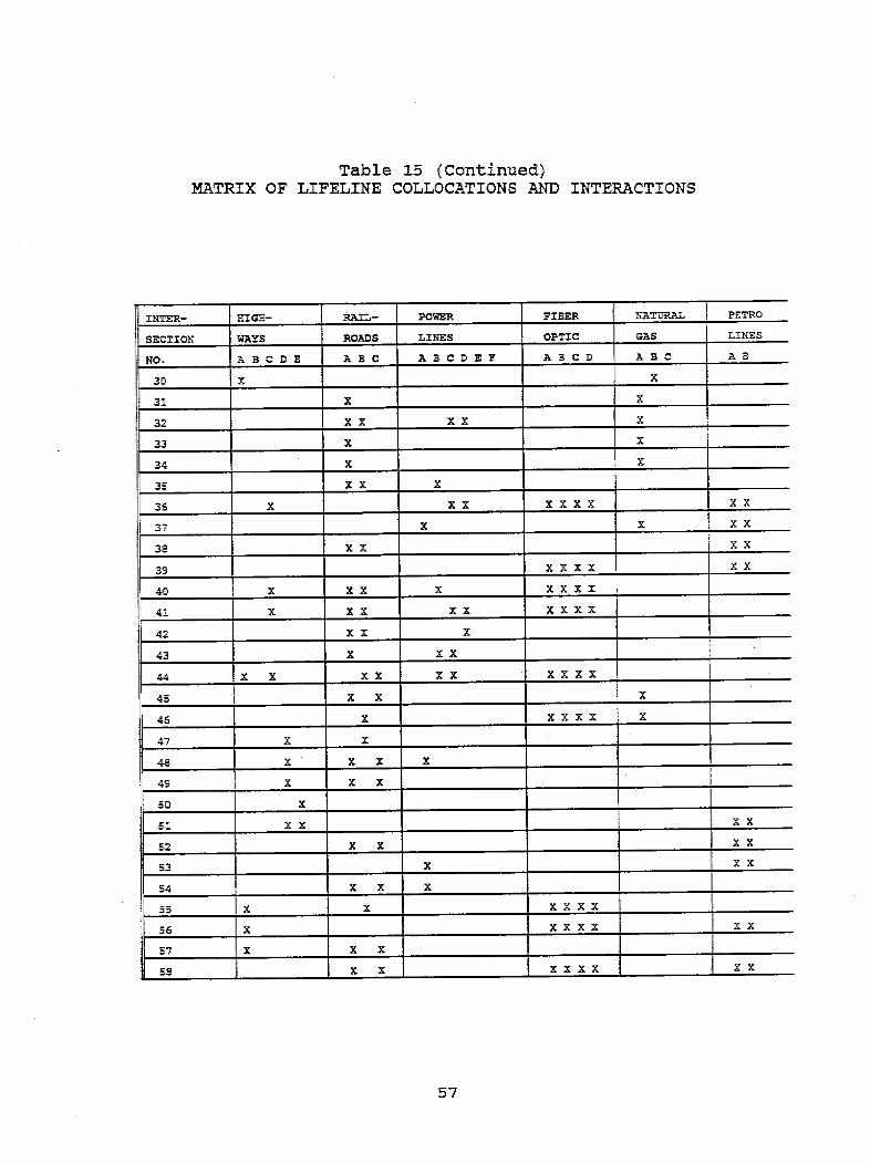
Table 15 (Continued)XATRIX OF LIFELINE COLLOCATIONS AND INTERACTIONS
INTER- HIGH- RAIL- POWER FIBER NATURAL PETRO
SECTION WAYS ROADS LINES OPTIC GAS LINES
NO. A B CD E A B C A B C D E F A B C D A B C A B
30 X X .
31 X _X
32 . xx xx x
33 X X X
34 X ,X _
35 _ _ _ _ x x H _ _ _
*36 XX XX x XX
37 X X XX
38 . XX ____ xx
3S~~~~~~~~~~~ XXXX XX
40 X XX X XXXX
. 41 X xX XX X X X __X
42 XX x
43 X XX
44 X X XX i XX XXXX
45 X X x X
46 X XXXX X
47 I X X
48 X X X X
49i X X X . -
s5 X
51 xx xx
52 . X X XX
53 X XX
54 X X X
55 X X ______ XXXX
56 x xxxx xx
57 X X X
58 X X ____________ XXXX ________ XX
57

Table 15 (Continued)MATRIX OF LIFELINE COLLOCATIONS AND INTERACTIONS
INTER- HIGH- RAIL-. POWER FIBER NATURAL PETRO
SECTION WAYS ROADS LINES OPTIC GAS LINES
NO. A B C D E A B C A B C D E F A B C D A B C A 3
59 X X X X X
601 X X xX X X X
62 x x x xxx X
63 __ _ _ _ X_ _ _ _ _ _
64 X X
65 X X
66 X ._. XX
67 XXX XX
68 X X _ _ _ _ _ _ _
69 X X
70 x x
71 = X '_== -
72s x x
73 xxx x x
74 x x xx x xx
75 1 I _ _ _ _ _
76 x x x x
77 81_X' X X X
7 8 I _ _ _ _ _ _ _ _ _ _ _ _ _ _ _ _ _ _ _ _
el2 x x x xx
84 .x x x x
86 X XX X
87 X X X X
58

Table 15 (Continued)MATRIX OF LIFELINE COLLOCATIONS AND INTERACTIONS
INTER- HIGH- RAIL- POWER FIBER NATURAL PETRO
SECTICON WAYS ROADS LINES OPTIC GAS LINES
NO. A S C D E A B C A 8 C D E F A 3 C D A BC A B
8_ X X X XX
.89 ______ HX XX X XX
90 X X X
NOT USEDX
93 H _ _ _ _ _ _ _ _ _ _ _ _
NOT USED = X XXX
96 X XX
93_ _ _ _ _ _ _ _ _ _ _ _ _ _ HX X X X97 ~X I X __ _ __ _
* 98 _ _ _ _ _ _ _ _ _ _ X _ _ _ _ _ _
99 _ _ _ _ _ _ _ _ _ _ _ _ _ _ _ X _ _ _ _ _
100 X X
101 XX
X - X
103 _ _ ,__ ,~~~~~~X X:
petroleum products pipelines. All of the buried lifelines
were found to have incurred damage state 7 (catastrophic) with
probabilities that the damage occurred of 40%. The assumed
collocation interaction was that the petroleum pipelines could
drain 1-2 miles of pipe but that no secondary fires or
explosions would occur. This contributed to an additional 30
day delay to the site before repair could commence, due to the
requirements to assure that fire conditions and environmental
concerns could be alleviated before work could start on the
individual lifelines. An additional 10 days of delay were
hypothesized due to the need to coordinate the work on so many
individual lifelines.
2. A second cluster exists along the Cajon Blvd. extension
into the Cajon Pass from north of the I-151I-215 interchange
to Blue Cut. There are two separate locations where
59

landslides (with a probability of occurrence of 45%) anu twoliquefaction areas (probability of occurrence of 20% and 40%)are possible, including eight separate collocation impactareas where there are collocated power lines, railroads, and anatural gas pipeline. At the two landslide areas along theCajon Blvd. extension (which was the prior highway 66 beforeI-15 was built), a natural gas pipeline and the railroads arelocated at the toe of the slide area, and landslide debris isexpected there. Debris removal for clearing the railroadwould be required before work on the pipeline (which islocated in the railroad right-of-way and sometimes under therail bed) could begin. The debris removal was assumed tocause a 30 day delay before work on repair of the pipelinecould occur.
3. At Blue Cut itself there is another landslide andliquefaction zone. Due to its proximity to the San Andreasfault rift zone, a 70% probability of occurrence wasestimated. At that location, a power line, a natural gaspipeline, and a railroad are in the flow area of the slide,which could cause the pipeline to surface and rupture as wellas to be covered with debris. The collocation damage scenarioassumed that an explosion and fire could result, increasingthe damage to the power line and its repair time by anadditional 20 days, compared to the delays described for theother slide area, to repair the more extensive damage the firecaused. The potential for landslides blocking the Cajon Creekwith a slide dam, and the subsequent impact on downstreamlifelines if the dam should catastrophically fail wereconsidered to be outside the scope of this study. At Blue Cutitself, the liquefaction zone has a 50% probability ofoccurrence.
4. In the San Andreas fault rift zone there are sixcollocation points that involve the power lines, therailroads, the fiber optics, a natural gas pipeline, the twopetroleum products pipelines, and the Cajon Blvd. extension.Fuel spills are assumed to require a 30 day delay foralleviating environmental and fire concerns. An additional 60day delay was assumed for the petroleum products pipelinesbecause the estimated extensive damage to their right-of-wayalong the fault trace will require regulatory review andacceptance before the pipeline can be worked on. Anadditional 30 day delay for the other lifelines was assumedbecause of the general congestion in the area. Since thefault displacement causes catastrophic failure of thelifelines, the collocation damage scenario does not assume anyfurther damage.
With these scenarios in mind, the collocation vulnerabilityanalysis was performed for each separate lifeline system.
60

Communication Lifelines
Figure 9 shows the communication lifeline routes in the study area.The location of the photographs presented in this. section of thereport are also shown on the figure. The microwave, radio, andcellular phone communication towers are sited such that they arenot collocated with other lifelines. Thus, they do not enter intothe analysis of the impact of collocation. The impact of degradedcommunications (if these towers should fail) on the ability torestore the other lifeline systems to acceptable deliveryconditions is beyond the scope of the present study..
There are five fiber optic systems located in the study area. Theyinclude American Telephone and Telegraph (AT&T), ContinentalTelephone (Contel), MCI Communications (MCI), WTG West (WTG,formerly WilTel), and US Sprint.
The individual fiber optic cables are multi-layered with an innerstructure that allows the cable to be pulled and maintained in astate of tension without placing tension on the individual glassfibers. This assembly is then wrapped with various insulatingmaterials, including a metal sheath. In the fall of 19.86, the U.S.Forest Service provided MCI and WTG right-of-ways on the basis thatthey would each provide two conduits and that each conduit would befour inches in diameter so that cables from two different systemscould be placed in each individual conduit (thus, provisions weremade to lay eight cable systems along the two routes through theForest Service land). Furthermorethe Forest Service required thatthe routes be combined as quickly as, practical. Thus, the MCI andContel systems enter the study area from the north along Baldy MesaRoad, while the AT&T, WTG, and US Sprint systems enter from thenorth along the access road to I-15. The routes join together justsouth of the separation of I-15N and 1-15S (about 1.8 miles northof the Cajon Junction of I-15 and Highway 138). From there theytravel together as a bundle of four conduits. Much of their routeis along the Cajon Blvd. extension where they are laid in themedian strip. Also routed along much of the median strip are thetwo petroleum products pipelines (the Cajon Blvd. extension was theformer divided highway 66, but only the western two lanes are stillmaintained for traffic). For the purposes of this study, the fiberoptic cables are analyzed as buried conduits. Because of theircollocation, if one conduit fails, all fail.
When the conduits, (which are normally buried) are routed to abridge location, they are generally brought to the surface and hungwith light anchors from the bridge. Figure 10 shows them on atypical bridge crossing on the abandoned portion of Highway 66;Figure 11 shows some of the details of the bridge hangers and theconditions of the conduits; Figure 12 shows them hung from ahighway culvert wall just south of Cajon Junction; Figure 13 showssome of the details of the wall anchors, near the culvert locationof Figure 12. Just south of the culvert shown in Figure 12 the
61

. II,3h U30.
Figure 9
SCALEo 1 Z S2 m
~m _
35 ~II =4.COMMUNICATIONLIFELINEROUTS. a
COMMUNICATION LIFELINE ROUTES
44EXPLANATION
-D I-s -_~~ a
... ... . .. ... ... . . .. ..., .. .. .......
INMWIATEPAVED MONV1AY
FM= 0MOtC CM&3
62
Is
.'a
Larger Scale FigureLocated at
End of Document

- - - - . ~~
Figure 10 Fiber Optic Conduits On A Bridge On The Abandoned Portion of Cajon Blvd. Extension

I
I
Figure 12 Fiber Optic Conduits On A Concrete Culvert That Passes Under 1-15
I
Figure 13 Wall Support Details For The Fiber Optic Conduits Of Figure 12
64

Figure 14 Surface Water Conditions Near The Toe Of The 1-15s Retaining Crib Wall
Figure 15 Fiber Optic Conduits Under a Heavy Water Pipe, Both On A Highway Bridge
65

fiber optic cables are buried at the toe of a crib wall used tosupport the southbound alignment of 1-15. Figure 14 shows thesurface water in this region, which was identified as a potentialliquefaction region. Figure 15 shows the conduits hung under awater distribution system pipe, both of which are supported from aroad bridge over a railroad. Other important collocations includewhere the conduits are buried near buried fuel pipelines, a numberof which are in liquefaction or landslide prone regions.
In all of these cases, the fiber optic cables are at potential riskbecause the light anchors used could be expected to fail due toshaking. The heavy water pipe just above the fiber optic cableconduit can be expected to fall on and fail those cables.
The analysis of the fiber optic cable systems indicates that theyare not at significant risk until the MMI values equal VIII ormore. In the Cajon Pass that occurs at liquefaction areas or atthe San Andreas fault where surface displacements of up to 12meters are anticipated. Thus, shaking damage is not expected to besignificant compared to displacement-related damage. However, thescreening method data base does not directly account for the lightanchors and the conditions of the conduits as shown in the figures.It is possible that they are more sensitive to shaking damage thanthe screening method predicts.
At the San Andreas fault location (just north of and close to BlueCut) the fiber optic conduits are not collocated with otherlifelines within the zone of influence of the lifeline. Thus, forpurposes of this study there is no collocation impact there.However, the large number of near by lifelines does suggest thatgeneral construction congestion could delay the permanent repair ofthe communication lifelines in this region. Also, it probablywould be possible to temporarily lay the fiber conduits on theground surface, restoring service on a temporary basis. Thesetypes of changes to the assumed restoration of service time arenoted, but they were not used in the present study to estimate theservice restoration time.
Four liquefaction regions have the potential to impact the fiberoptic systems. At the liquefaction region just southeast of the I-15/I-215 interchange, the fiber optic cables are in separate anddispersed conduits. However, two cable conduits cross this zonenear the railroad beds. One cable conduit crosses the 16-inchnatural gas pipeline and the 8-inch petroleum products pipeline,and then it runs parallel to the 8-inch line. Another cable conduitcrosses the liquefaction zone and is perpendicular to the 16-inchnatural gas pipeline, which is also in the liquefaction zone. Theliquefaction impact is calculated as a damage state 7(catastrophic) but it only has a 40% probability of occurring. Theconduit repair time in this region is hypothesized to triple, basedon the delays required to repair the natural gas and the petroleumproducts pipelines and the delays associated with the repair of the
66

nearby damaged I-15 and railroad bridges. This causes the fiberoptic conduits' most probable repair time to increase by about tendays.
In the second liquefaction region the four cable conduits arecollocated and they are parallel and next to the 8-inch and 14-inchpetroleum products pipelines. In this region they cross over the36-inch natural gas pipeline. The liquefaction impact is a damagestate 7 with a 20% probability of occurrence. The collocationdamage scenario assumed that the petroleum product pipelines wouldhave to be repaired before the fiber optic cables could be replacedwithin their conduits along their old route, causing a 55 day delayin being able to access the five fiber optic cables. Another 10days delay for equipment availability is expected. However, thelow probability of liquefaction resulted in the most probablerestoration time increasing by only about four days.
The third liquefaction zone is just south of Blue Cut. Thecollocated lifelines include the fiber optic conduits, fuelpipelines and a high voltage power line also crosses over theregion. The liquefaction probability at this locations isestimated at 50%. Most of the repair activities for the power linewill not impact the fiber optic cable conduit repair. The onlyimpact could come when the power lines directly over the conduitsare being worked on. The most probable restoration time increasedby only about 12 days.
The fourth liquefaction zone is where the fiber optic conduitscross the toe of an I-15 retaining wall crib and then are connectedalong the concrete culvert under I-15 (see Figures 13 and 14). Theconcrete culvert is a massive structure, and its damage is expectedto be small. Analysis of the crib wall found that its movementwould not substantially impact the highway, however, just partialmovement of the crib wall could severely damage the fiber opticcables. In such a case they could not be replaced permanentlyuntil the wall had been stabilized. Fortunately, the probabilityof liquefaction is.only 40% in this region, resulting in the 140day crib wall-induced delay becoming a 22 day most probablerestoration time increase for the fiber optic conduits.
Where the AT&T and WTG cables are hung from the bridge over theSouthern Pacific railroad is the final collocation damage locationwhere the collocation impacts were found to be serious (see Figure15). There, because the shaking intensity is only MMI=VII, notmuch damage would normally be expected to the cable conduit itself.However, the wall brace and anchor supports for the water pipe andthe fiber optic conduit are small and have not been sized forearthquake conditions. Thus, it was assumed that they failallowing the fiber optic conduit to sag. The heavier water pipewas assumed to fall on top of the fiber optic conduit which islocated directly under it, causing the fiber optic conduit torupture and fail. The probability of this, failure scenario is
67
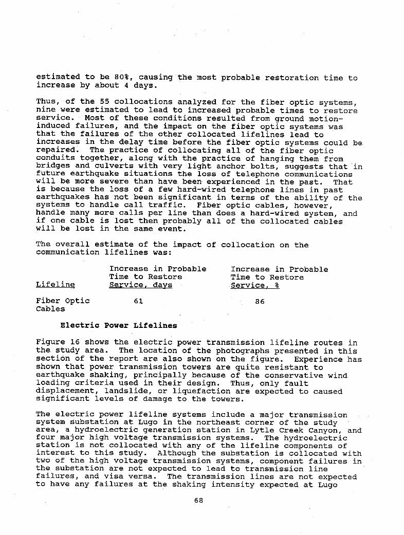
estimated to be 80%, causing the most probable restoration time toincrease by about 4 days.
Thus, of the 55 collocations analyzed for the fiber optic systems,nine were estimated to lead to increased probable times to restoreservice. Most of these conditions resulted from ground motion-induced failures, and the impact on the fiber optic systems wasthat the failures of the other collocated lifelines lead toincreases in the delay time before the fiber optic systems could berepaired. The practice of collocating all of the fiber opticconduits together, along with the practice of hanging them frombridges and culverts with very light anchor bolts, suggests that infuture earthquake situations the loss of telephone communicationswill be more severe than have been experienced in the past. Thatis because the loss of a few hard-wired telephone lines in pastearthquakes has not been significant in terms of the ability of thesystems to handle call traffic. Fiber optic cables, however,handle many more calls per line than does a hard-wired system, andif one cable is lost then probably all of the collocated cableswill be lost in the same event.
The overall estimate of the impact of collocation on thecommunication lifelines was:
Increase in Probable Increase in ProbableTime to Restore Time to Restore
Lifeline Service, days Service, %
Fiber Optic 61 86Cables
Electric Power Lifelines
Figure 16 shows the electric power transmission lifeline routes inthe study area. The location of the photographs presented in thissection of the report are also shown on the figure. Experience hasshown that power transmission towers are quite resistant toearthquake shaking, principally because of the conservative windloading criteria used in their design. Thus, only faultdisplacement, landslide, or liquefaction are expected to causedsignificant levels of damage to the towers.
The electric power lifeline systems include a major transmissionsystem substation at Lugo in the northeast corner of the studyarea, a hydroelectric generation station in Lytle Creek Canyon, andfour major high voltage transmission systems. The hydroelectricstation is not collocated with any of the lifeline components ofinterest to this study. Although the substation is collocated withtwo of the high voltage transmission systems, component failures inthe substation are not expected to lead to transmission linefailures, and visa versa. The transmission lines are not expectedto have any failures at the shaking intensity expected at Lugo
68

e III7 S1
Figure 16, EL
SCALEa I Z mum
e... ,-~ z AWLn=
fibU?'
iECTRIC POWER LIFELINE ROUTES
4'EXPLANATION
Larger Scale FigureLocated at
End of Document
-~ n-Is -~ INtK~Mh
- z . KVrD ActzrAX
--- --oM AS=
------- V-------- - -w A anUCrm
69
.1

(where MMI = VII). Thus, although the substation is a potential weak link in the overall electric power transmission system, the lack of collocation impacts means it was not be examined further in the present study.
In general, power transmission lines are not impacted directly by the other lifelines, as they are either above or otherwise outside of the zone of influence of the other lifelines. However, they can be impacted by construction delays or fires induced by the failure of other lifelines. The general tower design and footings used are quite rugged and earthquake resistant (resistant to shaking damage). There have been some cases when shaking has caused the lines themselves to gallop or vibrate, resulting in their coming close or even touching other lines routed on the same tower. The resulting arc and electrical short can cause fires and/or drop both lines from service. However, this failure mode is not addressed in the available data base and thus was not considered in
~~
'igure 17 A Landslide Scar With Power Towers In The Slide Area
the present study.
Transmission lines often traverse more rugged areas, and as such they are susceptible to landslide damage. Figure 17 shows two transmission towers located in an old landslide scar (the original towers were damaged in the landslide). This location is an important collocation site, as a buried natural gas transmission pipeline and the railroad tracts are located just below the slide area. Figure 18 shows the location of two high voltage power transmission tower systems, a buried natural gas transmission pipeline (shown by a surface marker), and the 8- and 14-inch buried petroleum products pipelines (also shown by a surface marker).
70

This location is in the fault rift zone of the San Andreas fault ( in Lone Pine Canyon). Figure 19 is a photograph from the same location looking in the opposite direction. It shows a transmission tower located at the edge of a steep ravine where it is subject to possible landslide failure . This general location (in
I
'igure 18 Power Lines, Natural Gas & Petroleum Products Pipelines Intersection Over the San Andreas Fault Rift Zone
the San Andreas fault and rift zone) is the most significant collocation condition for the electric and the fuel lifelines.
The Southern California Edison (SCE) 115 kV Arrowhead:Calelectric Shannin transmission line (located in the southeast corner of the study area) is routed through some local landslide and liquefaction zones, however, it is not collocated at those regions. Its other collocation impacts were negligible. In the northern section of the study area the SCE Lugo-Vincent two-line, 500 kV transmission lines traverse from Lug0 station west and then northwest. Because of the low shaking intensity (low for power lines), they only experience damage state 1 or 2. Thus, these two SCE transmission systems are not of interest for collocation impacts in the present study. There are, however, a Los Angeles Department of Water and Power (LADWP) two-line transmission system and a three-line SCE transmission line system that resulted in collocation impacts.
The LADWP Victorvil1e:Century 287.5 kV transmission line system (it has two full circuits) extends from the north (located at about the center of the northern boundary of the study area) to the south of the study region. from the Hoover Dam in Nevada to the Los Angles Basin. It has been upgraded in 1970, 1974 and 1980 to allow switching between the 287.5 and other 500 kV lines as well as to add new controls. Parts of the line have previously experience problems of interest to this
It was constructed in 1936 to transmit power
71
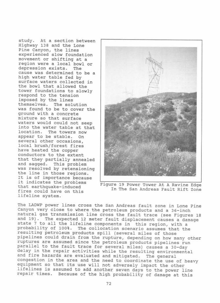
study. At a section betweenHighway 138 and the LonePine Canyon, the linesexperienced slow foundationmovement or shifting at aregion were a local bowl ordepression exists. Thecause was determined to be ahigh water table fed bysurface waters collected inthe bowl that allowed thetower foundations to slowlyrespond to the tensionimposed by the linesthemselves. The solutionwas found to be to cover theground with a concretemixture so that surfacewaters would could not seepinto the water table at thatlocation. The towers nowappear to be stable. Onseveral other occasions,local brush/forest fireshave heated the copperconductors to the extentthat they partially annealedand sagged. This problemwas resolved by retensioningthe line in those regions.It is of importance becauseit indicates the problemsthat earthquake-inducedfires could have on thislifeline system.
Figure 19 Power Tower At A Ravine EdgeIn The San Andreas Fault Rift Zone
The LADWP power lines cross the San Andreas fault zone in Lone PineCanyon very close to where the petroleum products and a 36-inchnatural gas transmission line cross the fault trace (see Figures 18and 19). The expected 12 meter fault displacement causes a damagestate 7 to all the lifeline components in this region, with aprobability of 100%. The collocation scenario assumes that theresulting petroleum products spill (several miles of thosepipelines could drain from the rupture, depending on how many otherruptures are assumed since the petroleum products pipelines runparallel to the fault trace for several miles) causes a 30-daydelay in the repair activities while the resulting environmentaland fire hazards are evaluated and mitigated. The generalcongestion in the area and the need to coordinate the use of heavyequipment so that its use will not adversely impact the otherlifelines is assumed to add another seven days to the power linerepair times. Because of the high probability of damage at this
72
, V; ,
I s
I
'7 k�I I' �4 ��

location, the probable restoration time increases by 37 days. Thisaccounts for about 75% of the collocation-induced delays in therestoration of service to the LADWP power lines.
The other significant collocation region for the LADWP power linesis also at Blue Cut. The power lines cross the eastern edge of alandslide zone, and at the toe of the zone at a lower elevation a36-inch natural gas pipeline is sited next to and in the right-of-way of a rail line. The probability of a slide in this region is
70%, it produces a power line damage state of 5 (heavy damage).The collocation scenario includes a seven day period while the gasline is prepared and tested for leaks, and a increase in damagestate to level 6 because of potential natural gas pipeline failureimpacts. That scenario increased the repair time from 49 to 66days and the net impact on the change in restoration time was about12 days.
There are three 500 kV circuits on SCE's Lugo - Mira Loma system.They were installed in the early 1960s for about 300 kV service andupgraded to 500 kV service in the early 1970s. Line 3 was added in1983.
Line 1 is to the west, line 2 is in the center, and line 3 is theeastern line. Line 1 is routed south by southwest from the Lugosubstation. Lines 2 & 3 leave Lugo station on a single towersystem for about 1.5 miles, then they divide into two separatetower systems. The power lines cross the railroad lines a shortdistance before they cross Highway 138. From there they headgenerally south until they cross I-15. In this high desert regionthe only earthquake load comes from shaking characterized by MMI =
VII. At that intensity there is no appreciable damage to thetowers or the lines, and no collocation impacts were hypothesized.
At the I-15 crossing, lines 1 & 2 cross at the northern boundary of
a local liquefaction zone. Because their power towers are locatedon local hill tops in this region, it is assumed that there are noimpacts due to the liquefaction or due to collocation. However,they cross near a concrete culvert that crosses under the highway.At the culvert (see Figure 12) location there is also a metal cribwall (see Figure 13) that provides support to the road bed, the
fiber optic cables cross at the same location, there are tworailroad bridges in the downstream path from the run off thatpasses through the culvert, and there is a 36-inch natural gas linewhich crosses I-15 in the same area. In addition, the crossing isin an area of high water table and of surface water, indicating apotential liquefaction zone. Although the power towers and linesare not expected to experience damage at this location, they willcause some delays in responding to damage on the other lifelinesbecause of the need to work with large cranes and other equipmentthat could get close enough to the power lines to cause the needfor caution to avoid potentials for electrocutions, etc... Line 3crosses I-15 further south and is not impacted by the crowded
73

conditions described above.
After crossing I-15, lines 1 & 2 are routed as parallel lines.Where they cross the San Andreas fault they will experience damagestate 7 due to the 12 meter displacement expected at the faulttrace. The two lines pose a collocation potential that is assumedto increase their repair time by 15 days. This increases theirprobable restoration time by 15 days because of the highprobability that the large fault displacement will occur. Afterthis, the lines again separate, with line 1 heading south, and line2 heading southeast until it joins with line 3 at Blue Cut.
As line 1 heads south it enters a liquefaction zone that is northand abuts against a landslide zone. Within the liquefaction zoneit crosses over the two petroleum product pipelines, the fiberoptic conduits, and Cajon Blvd. extension. Near the boundarybetween the liquefaction and landslide zones it crosses over a 36-inch natural gas pipeline that is itself next to and in the right-of-way of a railroad line. The liquefaction zone results in a 50%probability of damage state 7 occurring to the power towers. Thecollocation scenario is a 20 day delay due to the generalcongestion in the region, which results in a probable delay inrestoration of 4 days. There are no other significant collocationregions for line 1 further south along its route.
After they join together, lines 2 & 3 head in a south by southeast-direction. They cross the Cajon Blvd. extension at the northernboundary of a local liquefaction zone and head up the steep slopesto the higher elevations of the San Gabriel Mountains. Just abovethe Cajon Pass floor as they rise into the mountains they enter alandslide zone. Figure 17 shows that in the past they haveexperienced slides that have required extensive repair. At the toeof the slide a 36-inch natural gas pipeline is located next to andin the right-of-way of a railroad bed. The landslide causes adamage state 5 (with a probability of 45%). It is assumed that thecongestion and the need to shut down the power line when the gaspipeline is to be tested for leaks will add 40 days to the repairof the power towers. This makes their probable restoration timeincrease by nine days at this location.
The typical collocation damage scenario is that other lifelineshave a minor physical impact on power lines because the power linesare above or removed from the zone of influence of the otherlifelines. However, when fuel-based lifelines are involved, theycan cause important delays in the power line restoration. This isto assure that the power lines do not become a source of ignitionfor the fuel. Also, when the other lifelines are directly underthe power lines, the expected use of temporary support towers maynot be acceptable because of the increased risk of electrocutionwhen other large repair equipment is operated near a temporarytower. As was the case for the communication lifelines, groundmovement was the principal cause of electrical transmission
74

lifeline damage.
One hundred and four collocations involving the electric power lifelines were analyzed. The overall estimate of the impact of collocation on the electric power lifelines in the Cajon Pass was:
Lifeline
Increase in Probable Increase in Probable Time to Restore Time to Restore Service. days Service. %
Los Angeles Dept. 49 of Water & Power
Southern California 19 Edison Co. Line #1
Southern California 28 Edison Co. Line #2&3
28
10
13
Fuel Pipeline Lifelines
Figure 20 shows the fuel pipeline lifeline routes in the study area. The location of the photographs presented in this section of the report are also shown on the figure. The lifelines include one 8 - and one 16-inch petroleum products pipelines, three 36- and one 16-inch natural gas pipelines, and the associated valves for each line. Modern buried pipelines of the type installed at Cajon Pass are very resistant to shaking damage. Thus, the earthquake conditions of most interest for the pipelines are the conditions where ground movement is expected. However, when they are buried next to or under Figure 21 Typical Long Open Span On The 36-Inch another Natural Gas Pipeline
7 5

7l a a s 1 17§i 17 PI It Ff I J .
Figure 20, FUEL PIPELINE LIFELINE ROUTESSCALE
0 l 2 I o rk
EXPLANATION
- ~ 1-15 INTIESAha PAID SUBWAY
- …---0------ 0 - PZTUOLIM PRODUCT mPWUNE----------------- 0-- NATURAL DU PhP
0 0 0ALM
Larger Scale r igureLocated at
End of Document
76
*a.I
a
aC.
Ž .1-611
if - V�-- - -
they are withtherailroads),there is anadditionalconcern thatheavyequipmentused toremove debrisor otherwiserestore therailroadlifelinecould lead topipe walldamage of thenearby buriedfuelpipeline.
Because they Figure 22 Two Natural Gas Pipelines Near Highway 138,are buried, One Buried, One Exposedthere are noconvenientfeatures that can be shown with photographs. However, there are 18locations along the route of the western most 36-inch natural gaspipeline that are exposed spans which range from 10 to 138 feet inlength. Figure 21 shows one of the longer spans across a dry creekbed north of Highway 138 and east of I-15. Figure 22 shows alocation about 40 feet from the recently realigned Highway 138. Atthat location two 36-inch natural gas pipelines are routed parallelto each other. The line on the left is exposed, the one on the
right is buried and marked with the surface sign. In general, openspans are estimated to increase the potential shaking damage stateby up to 1 level, compared to a buried pipeline damage statecondition.
When the pipelines cross under railroads, roadbeds, and sometimespower line rights-of-way, many of the right-of-way owners requiredthe pipeline to be cased inside a larger pipe in the belief thatthis adds safety and/or it reduces the lifeline interactions ifdamage on one lifeline should occur (there is a current technicalquestion whether the casing increases or reduces the overall safetyof the crossing). Figure 23 shows a location where a 36-inchnatural gas transmission line crosses under two different railbeds. One railroad requires the use of the extra casing, the otherdoes not. If the use of a casing increases the safety of thecrossing, the close proximity of the railroads means that the extrabenefit is lost. If the use of a casing decreases the safety ofthe crossing, then the railroad expecting extra safety has not
77
1 4 -F � 1 i ran f = a

achieved it because of the close proximity in this situation.
Two of the most critical collocations involving fuel pipelines were shown in Figures 17 and 18. In Figure 17 the pipeline and the railroads are located directly below a landslide prone area that includes electrical transmission towers. Figure 18 shows that both types of fuel pipelines and high voltage electrical transmission systems all cross the San Andreas fault rift zone at approximately the same location. The results of these conditions are discussed below.
The western most 36-inch natural gas pipeline from valve station 14 (near the Cajon railroad summit east of the I-lS/Highway 138 interchange) south to the end of the study area was installed in 1960. The eastern most 36-inch natural gas pipeline was installed in 1966. They operate at a mean operating pressure of 845 psig. The 16-inch distribution supply line branches off of those lines at Valve 15 (south and west of the 1-15/1-215 interchange) and provides service to San Bernardino. It operates at a mean operating pressure of 350 psig. The line from the north of the study area (along Baldy Mesa Road) to valve station 14 was installed in 1976. It operates at a mean operating pressure of 936 psig. All of the lines were arc welded and constructed from high grade steel pipe. They deliver 0.6-1.0 billion cubic feet of natural gas per day.
The 8-inch petroleum products pipeline was installed in 1960 and the 14-inch line was installed in 1969. In 1980, several miles of the 8-inch line were abandoned and a new line was routed from the west side of Cajon Creek to join the 14-inch line on the east side. On the east side of Cajon Creek they are routed along the Cajon Blvd. extension. The lines transport a number of refined products, the
?igure 23 Natural Gas Pipeline Crossing Under Railroad Beds
78

transport a number of refined products, the principal ones beinggasoline and jet fuel. They are made of high grade carbon steel.They operate at 1060-1690 psig. The lines pump about 30,000barrels of fuel per day.
Most of the pipeline highway or railroad bed crossings are casedcrossings. However, none of the Southern Pacific crossings arecased, and a few of the I-15 and Highway 138 crossings are uncased.That occurred because the Southern Pacific did not require casingwhen they authorized the right-of-way crossing, and when I-15replaced Highway 66 and when Highway 138 was recently realigned (in1990-1991) they did not follow all of the old routes. At newcrossings the pipeline was already installed, and new casings werenot required to be retrofit.
In the regions of MMI = VII or less, the shaking damage state for aburied gas or petroleum products transmission line is 1, and nocollocation damage is estimated except for unusual conditions to bedescribed below.
Following the pipelines from the center of the northern part of thestudy area and heading south, the first location for significantdamage occurs at the crossing of the San Andreas fault. Here the12 meter fault displacement is assumed to rupture the lines. Thelocation includes the 36-inch natural gas pipeline and the twopetroleum products pipelines (all of which rupture) and theVictorville-Century 287.5 kV lines 1 and 2. The damage scenarioincludes assuming that an explosion/fire occurs in addition to thedischarge of petroleum products. The need to mitigate the impactof the fire and adverse environmental conditions and the delayscaused by the general congestion in the area results in an assumed37 day delay before restoration work can begin. Because of thehigh probability (100%) of the damage state, the incrementalincrease in the lifeline restoration time is also 37 days.
At Blue Cut the natural gas pipeline is next to the railroad bedand at the toe of a landslide area. High voltage power lines arelocated above the gas line in the slide area. A damage state 4 ispredicted for the pipeline. The heavy equipment used to clear therailroad bed is assumed to increase the damage state to level 5.This increases the pipeline repair time by 18 days, and the debrisclean up adds another 20 day delay. The general congestion adds a7 day delay. This results in a change in the most probablerestoration time of 12 days. Further south the pipeline followsthe railroad bed along the west edge of Cajon Creek. About 4 milesfurther south, the pipeline and railroad are again at the toe of alandslide region. In this case only the 18 day increase in repairtime and the 20 day debris removal delay are assumed. This resultsin an 8 day increase in the probable restoration time for thatpipeline, for a total increase in time of 20 days.
Moving from the north to the south, the eastern most natural gas
79
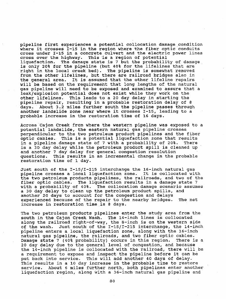
pipeline first experiences a potential collocation damage conditionwhere it crosses I-15 in the region where the fiber optic conduitscross under I-15 in a concrete culvert and the electric power linescross over the highway. This is a region of potentialliquefaction. The damage state is 7 but the probability of damageis only 20% for the pipeline (but 40% for the lifelines that areright in the local creek bed). The pipeline is somewhat removedfrom the other lifelines, but there are railroad bridges also inthe general area. It is assumed that the other lifeline repairswill be based on the requirement that long lengths of the naturalgas pipeline will need to be exposed and examined to assure that aleak/explosion potential does not exist while they work on theother lifelines. This leads to a 20 day delay in starting thepipeline repair, resulting in a probable restoration delay of 8days. About 3.2 miles further south the pipeline passes throughanother landslide zone near where it crosses I-15, leading to aprobable increase in the restoration time of 16 days.
Across Cajon Creek from where the western pipeline was exposed to apotential landslide, the eastern natural gas pipeline crossesperpendicular to the two petroleum product pipelines and the fiberoptic cables. This is a potential liquefaction zone that resultsin a pipeline damage state of 7 with a probability of 20%. Thereis a 30 day delay while the petroleum product spill is cleaned upand another 7 day delay for general congestion resolutionquestions. This results in an incremental change in the probablerestoration time of 2 day.
Just south of the I-15/I-215 interchange the 16-inch natural gaspipeline crosses a local liquefaction zone. It is collocated withthe two petroleum products pipelines, the railroads, and two of thefiber optic cables. The liquefaction results in a damage state 7with a probability of 40%. The collocation damage scenario assumesa 30 day delay to clean up the petroleum product spills, andanother 20 days to account for the congestion and delaysexperienced because of the repair to the nearby bridges. The netincrease in restoration time is 8 days.
The two petroleum products pipelines enter the study area from thesouth in the Cajon Creek Wash. The 14-inch lines is collocatedalong the railroad right-of-way, the 8-inch is on the western sideof the wash. Just south of the I-15/I-215 interchange, the 14-inchpipeline enters a local liquefaction zone, along with the 16-inchnatural gas pipeline, the railroads, and two fiber optic cables.Damage state 7 (40% probability) occurs in this region. There is a20 day delay due to the general level of congestion, and becausethe 14-inch pipeline is collocated with the railroad, there will bea requirement to expose and inspect the pipeline before it can beput back into service. This will add another 40 days of delay.This results in a 10 day increase in the probable time to restoreservice. About 6 miles further north, both pipelines enter anotherliquefaction region, along with a 36-inch natural gas pipeline and
80
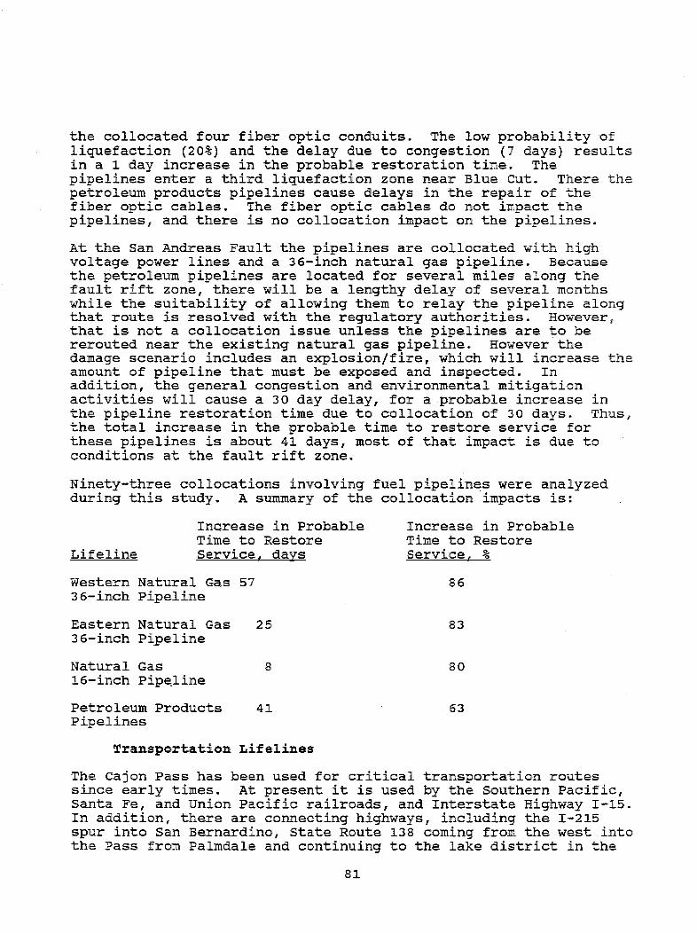
the collocated four fiber optic conduits. The low probability ofliquefaction (20%) and the delay due to congestion (7 days) resultsin a 1 day increase in the probable restoration time. Thepipelines enter a third liquefaction zone near Blue Cut. There thepetroleum products pipelines cause delays in the repair of thefiber optic cables. The fiber optic cables do not impact thepipelines, and there is no collocation impact on the pipelines.
At the San Andreas Fault the pipelines are collocated with highvoltage power lines and a 36-inch natural gas pipeline. Becausethe petroleum pipelines are located for several miles along thefault rift zone, there will be a lengthy delay of several monthswhile the suitability of allowing them to relay the pipeline alongthat route is resolved with the regulatory authorities. However,that is not a collocation issue unless the pipelines are to bererouted near the existing natural gas pipeline. However thedamage scenario includes an explosion/fire, which will increase theamount of pipeline that must be exposed and inspected. Inaddition, the general congestion and environmental mitigationactivities will cause a 30 day delay, for a probable increase inthe pipeline restoration time due to collocation of 30 days. Thus,the total increase in the probable time to restore service forthese pipelines is about 41 days, most of that impact is due toconditions at the fault rift zone.
Ninety-three collocations involving fuel pipelines were analyzedduring this study. A summary of the collocation impacts is:
Increase in Probable Increase in ProbableTime to Restore Time to Restore
Lifeline Service, days Service. ,
Western Natural Gas 57 8636-inch Pipeline
Eastern Natural Gas 25 8336-inch Pipeline
Natural Gas 8 8016-inch Pipeline
Petroleum Products 41 63Pipelines
Transportation Lifelines
The Cajon Pass has been used for critical transportation routessince early times. At present it is used by the Southern Pacific,Santa Fe, and Union Pacific railroads, and Interstate Highway I-15.In addition, there are connecting highways, including the I-215spur into San Bernardino, State Route 138 coming from the west intothe Pass from Palmdale and continuing to the lake district in the
81

east, and a partially abandoned section of old Federal highway U.S.66, now called the Cajon Blvd. extension. The routes of theselifelines in Cajon Pass is shown in Figure 24. The location of thephotographs presented in this section of the report are also shownon the figure.
Because these routes are discontinuous in the sense that eachbridge, each change in MMI intensity, and each local liquefactionor landslide area must be separately checked. The railroads had tobe segmented into 30 separate analysis sections and the I-15highway into 36 separate analysis sections. During thevulnerability analysis of these facilities, it was necessary toconsider some extension outside the study area in order to providerealistic estimates of time to restore service. In the case of theSouthern Pacific Railroad, for example, the route considered wasextended to the Highland Boulevard over-crossing in San Bernardino.The assumptions with regard to equipment available to make repairsdiffers from that used for the pipeline and communication lifelinesin that it is assumed that the railroads and highways both havelocal active maintenance yards with their own heavy equipment forconstruction activities. While some of this may be pressed intoservice for life saving activities in the early emergency phase, itis not likely that this will prevent immediate inspection andreconnaissance. Therefore, no delay time waiting for equipmentavailability was assumed.
Moving this equipment to the most critical sites along thetransportation lifeline, on the other hand, may present asignificant problem of access because the equipment must move alongthe lifeline facility itself. In each analysis, it is firstassumed that the equipment must work from one end or the other ofthe Cajon Pass, repairing each section as it goes before it canreach the next section. The probable access time to a givensection is the sum of the products of times to repair all sectionsup to that point multiplied by their respective probability ofdamage. For the conditions existing in the Cajon Pass, this leadsto very long access times for those sections remote from the Passentrances. A second analysis was therefore made in which thepossibility of construction of temporary by-passes around damagedsections to permit the access of construction equipment to morecritical sites was considered (this, of course, only applies to thehighway portions of the transportation lifelines). The access timeto a given site in that situation became the sum of the products ofthe by-pass times and the probability that each of them is requiredbecause of the damage-in the section being analyzed. Some of thehighway bridges on I-15 have built in by-pass capability, sincethey are part of "diamond" interchanges in which the ramps mayserve this purpose. In the generally dry conditions of Cajon Pass,it is possible in many cases to simply drive across country intracked vehicles and lightly loaded four wheel drive trucks. Someroad bed material would need to be placed to support heavy highwayconstruction equipment.
82

.- I
; 1. . I
Figure 24,
SCALEG 1 2 MU=
i * -mrs
EXPLANATION
, .117 =
TRANSPORTATION LIFELINE ROUTES
'4 Larger Scale FigureLocated at
End ofDocument-~ I-Is
-2 PATtI GIWAYramrod 83
* r

The purposeof these
as ,4 nA o I-.access timeanalyses wasto find thecriticaltotal timefor thelifelinesection beingevaluated,that is, thetime to gainaccess to thesite withrepairequipmentplus the timeto carry outthe neededrepairs. Asin the case Figure 25 I-15 Bridge Over The Railroads In Cajon Wash
and powerlines, eachlifeline was first divided into sections, such that the conditionswithin eachsection werera-m = n ;] r% l v l. I
homogeneous.Because ofthe presenceof manybridges onthe highwaysandrailroads,this leads tomore sectionsfor theroughly 25miles oflength ofeach separatetransportationsystem.Prior to thedetailedanalysis of
- I- -tne lifeline Isection being Figure 26 I-15 Bridge Over Cajon Wash
84

considered, the Bridge Vulnerability Index of each of these structures had to be determined, and the probable extent and type of damage to each postulated.
The highway bridges along Interstate 1-15 were, for the most part, built in the late 1 9 6 0 f s , except for the section over Lytle Creek Wash. Although they are in an area generally considered to be IfCalifornia region 7", the status of retrofit is somewhat irregular. In this analysis, they are considered to be "California region 3-6" until proved to qualify for the higher degree of safety. Nevertheless, none of these bridges are expected to completely collapse, although partial collapse of several is possible. The 1-15 bridge over the railway lines (Figure 25) and the high level 1-15 bridge over Cajon Wash (Figure 26) are vulnerable, and there is some possibility of the partial collapse of the steel girders over 1-15 at its junction with highway 138 (Figure 27).
Many of the railroad bridges in the Cajon Pass are over 50 years old, but most are in relatively good condition. As noted in the discussion of the development of the Bridge Vulnerability Index, many of these bridges have inherent resistance to lateral loads. There are, however, several multiple simple span bridges over poor soil conditions (including possible liquefaction), such as both the Southern Pacific and Santa Fe bridges over the lower end of Cajon Wash (Figure 28). There are several more such crossings over the Cajon Creek and its branches. There is also a large two span, through plate, girder bridge on the Southern Pacific railroad over Highway 138 which is sharply skewed, and which has bearings which are vulnerable to loss (Figure 29). It is expected that the multiple span structures will have one or more spans dislodged where they are sub] ected Figure 27 Highway 138 Bridge Over 1-15
85

Figure 28 Railroad Bridges In Cajon Wash (-15 BridgeIn The Background)
Figure 29 Railroad Bridge Over Highway 138(Collapse Expected)
86
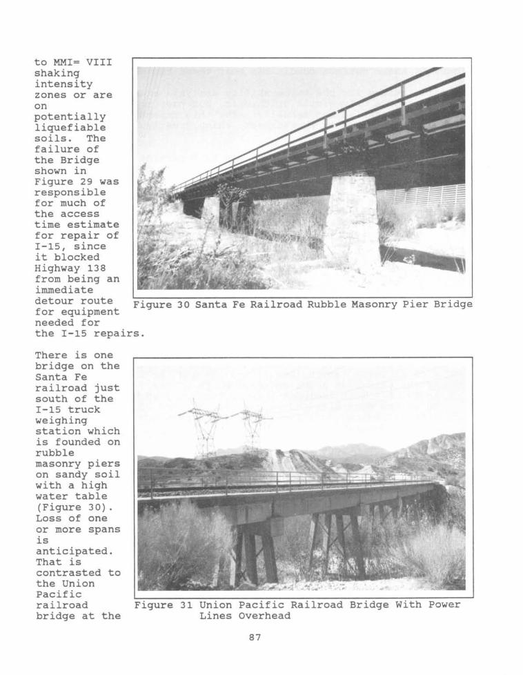
to MMI= VIII shaking intensity zones or are on potentially liquefiable soils. The failure of the Bridge shown in Figure 2 9 was responsible for much of the access time estimate for repair of 1-15, since it blocked Highway 138 from being an immediate detour route for equipment needed for
r
the 1-15 repairs.
Figure 30 Santa Fe Railroad Rubble Masonry Pier Bridge
There is one bridge on the Santa Fe railroad just south of the 1-15 truck weighing station which is founded on rubble masonry piers on sandy soil with a high water table (Figure 30). Loss of one or more spans is anticipated. That is contrasted to the Union Pacific railroad bridge at the
r:
I
"igure 31 Union Pacific Railroad Bridge With Power Lines Overhead
87

same location (Figure 31) which has steel column, pile piers.Figure 14 shows surface conditions near these two bridges.
The calculations for the vulnerability analysis and time to restoreservice involve only simple arithmetic, but they are quite timeconsuming if carried out manually. For this report, the analyseswere done on a computer spreadsheet, which greatly aided an orderlyand efficient approach.
The primary objective of the study was to determine how the timesto restore full service would be affected by the collocation ofseveral types of lifelines in the same congested corridor. Theinteraction scenarios have been discussed in this report in earliersections. There are, however additional problems because of thehighway-railroad interactions. For the Cajon Pass application,these interactions occur at the same general areas as thepreviously identified critical clusters:
(1) The area near the liquefiable zone just south of thehighway I-15 crossing over the railroads and the Cajon Wash,near the junction with I-215. This includes intersectionpoints 8, 9, 10, 11, 13, 14, 15, 16, 18, and 19. A partialcollapse of highway bridge No. 54-0818 over the three raillines adds to the problems at this location. A delay time of30 days due to this bridge problem (Figure 25) was added tothe previously noted 30 day delay due to pipeline damage andhazards.
(2) The section of the steep slide prone slopes along the westside of Cajon Canyon (see Figure 17) and the liquefiable zoneon the east side about one mile north of the junction of I-15an I-215. This includes intersections 22, 25, 26, 27, 28, 29,30 on the east side and 31, 32, 33, 34, and 35 on the westside of the canyon. The 30 day delay previously establishedappears adequate.
(3) The conditions in Blue Cut are so congested, combined withthe expected explosion and/or fire, that an increase in theexpected damage states for the railroads by one level isjustified. Intersections 38, 39, 93, and 99 are involved. A60 day delay in access is also assumed.
(4) At the San Andreas fault zone, intersections 37, 40, 41,and 91 are involved. Problems with fuel pipelines and powerlines have already been noted. The 30 day delay in initiatingrepairs to other lifelines was applied to the railroads.
(5) The area just north of the section of Highway 138 and westof Highway I-15. Problems with pipelines and power lines havealready been noted at intersection points 47, 48, 49, 51, 52,and 53. There is also a possibility of partial collapse ofthe Southern Pacific railroad bridge over Highway 138 (Figure
88
29). An additional delay time of 30 days was added for accessinvolving this bridge, over and above the 30 days to clearfire hazards related to pipeline damage.
(6) There are several other minor critical areas:
(a) The area just west and south of the I-15 truckweighing station. The crib retaining wall could slump(see Figure 14). The principle effect is on SouthernPacific railroad sections 15 (westbound) and 24(eastbound). A 30 day delay was assumed.
(b) Highway Structures 0796, 0797 and 0827 which carry1-15 over the rail lines at Alray and Gish atintersections 55 and 57 (Figure 32). These structuresmay only be lightly damaged, but a 10 day delay inrailroad access is assumed to permit time for inspectionand temporary shoring if required.
(c) The I-15 bridge 0664 (Figure 33) over the SouthernPacific tracks north of the pass at intersection 83 isexpected to be lightly damaged, but 10 days delay isallowed for inspection (also see Figure 15 which showsdetails of this bridge).
The effect of these collocation delays on the restoration of thetransportation lifelines was evaluated by making a analysis withcollocation assumed. This is a "second pass" analysis with thespreadsheet. A special problem developed in reassessment of thealternate route by way of highway 138, in that access to theconnection point on the Santa Fe was blocked by the expectedpartial bridge collapse on the Southern Pacific. For this reasonthe delay time associated with this problem was added to theprevious estimated time to reach the connection point, that is 10days plus 60 days delay time. This gives 70 days. The cumulativeaccess times for this route were then computed as before, workingboth ways from this point.
A summary of the results of the study are presented below.
Increase in Probable Increase in ProbableTime to Restore Time to Restore
Lifeline Service, days Service, %
Highway I-15 35 22
Southern Pacific 17 8Railroad
Atcheson Topeka & 85 33Santa Fe Railroad
89

The smallerpercent
increase inItime to lrestore l
c~ or rnF n^f ;:>ej v. V WU LvL
the SouthernPacificrailroadcompared tothe othertransportationlifelines.is due inpart to itsmorefavorablelocation withrespect tootherlifelines;but it shouldalso be noted Figure 32 Typical I-15 Box Bridge Over the Railroads
probablepartial collapse of one the bridges on this line contributes tolarge access4 4 ma --- , ; oL L But: L t: L^ :for theothers.
90
Figure 33 I-15 & Access Road Bridges Over the SouthernPacific Railroad
5.3 Chapter 5.0 Bibliography
1. P. Lowe, C. Scheffey, and P. Lam, "Inventory of Lifelines in
the Cajon Pass, California", ITI FEMA CP 120190, August 1991.
2. R. Greensfelder, "Maximum Credible Rock Acceleration From
Earthquakes in California", California Division of Mines and
Geology Map Sheet 23, 1974.
3. T. Hanks, "t The National Earthquake Hazards Reduction Program -
Scientific Status", U.S. Geological Survey Bulletin 1652,
1985.
4. J. Evernden, et. al., "Interpretation of Seismic Intensity
Data", Bulletin of the Seismological Society of America, V.
63, 1973.
5. J. Evernden, et. al.., "Seismic Intensities of Earthquakes of
Conterminous United States - Their Predications and
Interpretations", U.S. Geological Survey Professional Paper
1223, 1981.
6. J. Davis, et. al., "Earthquake Planning Scenario for a
Magnitude 8.3 Earthquake on the San Andreas Fault in Southern
California", California Division of Mines and Geology, Special
Publication 60, 1982.
7. S. Algermissen, et. al., "Development of a Technique for the
Rapid Estimation of Earthquake Loses", U.S. Geological Survey
Open File Report 78-441, 1978.
8. E. Bertugno and T. Spittler, "Geologic Map of the San
Bernardino Quadrangle", California Division of Mines and
Geology Geologic Map Series, Map No. 3A (Geology), 1986.
6.0 FUTURE STUDY NEEDS
Recognizing that this is the first comprehensive analysis of the
impact of lifeline collocation on the individual lifeline'svulnerability, it is recommended that the follow-on studies, be
performed.
1. The collocation analysis should be repeated at anotherlocation outside of California. It will provide informationon the following items:
Is there enough data available to conduct the analysis,or was the data base available in California unique?
Can the methods suggested by Rojahn to adjust theCalifornia data to other regions be applied to developreasonable results?
91

The site can include water and sewer systems orreservoirs to assure that the collocation analysis methodcan properly treat the impacts of these lifelines, whichwere not available at the Cajon Pass.
The study can check the suitability of the LSI-MMIrelationship developed for analyzing liquefaction-induceddamage, the Bridge Vulnerability Index method, and thelifeline zones of influence, all of which were developedwith the Cajon Pass situation in mind.
If possible, the study site should include lifelinepassage over a large water body, or at least over wetground. This will help clarify the impacts of equipmentand material access time compared to lifeline repairtime, as the dry ground of the Cajon Pass did not imposevery restrictive "detour" conditions.
2. In parallel with the above study to further refine thecollocation analysis method, a second study is warranted. Itshould focus on presenting the material to a broad audience.Special emphasis should be given to contacting lifeline ownersand operators to discuss the study and the results obtained.Their perspective and response should provide valuableinformation on where improvements in the analysis method wouldclarify important issues that relate to the siting oflifelines in "lifeline corridors". It should also helpidentify mitigation approaches that reflect the operationaland economic needs of the lifeline providers.
3. A longer term study is needed to provide more detailed dataand expert opinion for lifelines. Most of the current dataemphasizes earthquake impacts on buildings and secondly onbridges. Most of the present data (including most of thelifeline data) in the data bases were obtained from thebuilding and bridge technical sectors. An new study toexamine the present data base presented in ATC-13, but withfull emphasis on lifelines, should be undertaken to allow thelifeline portions of earthquake analysis to have the samelevel of technical input that buildings and structurespresently have.
92
Appendix A
Modified Mercalli Intensity (MMI) Index Scale
93

Modified MercaWli (MM) Intensity Scale *
I. Not felt-or, except rarely under especially favorable Circumsean e.. UJndercertain conditions, at and outside the boundary of the ares In whicha great shock is felt:
sometimes birds, animals, reported uneasy o, disturbed;sometimes dizzines or nausea experienced;sometimes trees1 structures, liquids, bodies of water, may sway--doorsmayo swing, very slowly.
II. Felt indoon by few, especially on upper foors, or by sensitive or nervouspersons.
Also, *s in grade I, but often more noticeably:sometimes hanging objects may swing,' especially -ben delkcately
suspended;sometimes trees, structures, lquids, bodies of water, may sway, 'doors
may swing, very slowly;sometimes birds, animals, reported uneasy or disturbed;sometimes dizziness or nausea experienced.
III. Felt indoors by several, motion usually rapid vibration.Sometimes not recognized to be in earthquake at first.Duration estimated in some cases.Vibration like that due to pasing of light, or lightly loaded trucks, or
heavy trucks some distance away.Hanging objects may swing slightly.Movements may be appreciable on upper levels of tall structures.Rocked standing motor car slightly.
rV. Felt indoors by many, outdoors by few.Awakened few, expecillly light sleepers.Frightened no one, unless apprehensive from previous experience.Vibration like that due to passing of heavy, or teavily loaded trucks.Sensation like heavy body striking building, or falling of heavy objects
inside.Rattling of dishes) windowg, doors; glassware and crockery clink and
clash.Creaking of walsa frame, especially in the upper range of this grade.Hanging objects swung, in numerous inttances.Disturbed liquids in open vessels slightly.Rocked standing motor cars noticeably.
V. Felt indoors by practically al, outdoors by many or most: outdoorsdirection estimated.
Awakened many, or most.Frightened few-slight excitement, a few ran outdoors.Buildings trembled throughout.Broke dishes, glassware, o some extent.Cracked windows-in some cases, but not Kenerally.Overturned vases, small or unstable objects, in many Instances, wiLt
ocecaional fall.Hanging objects, doors, swing generally or considerably.Knocked pictures against wlls, or swung them out of place.Opened, or closed, doors, shutters, abruptly.Pendulum clocks stopped,. started, or ran fast, or slow.Moved small objects, furnishings, the latter to slight extenLtSpilled liquids in small amounta from well-filled open containers.Trees, bushes, shaken slightly.
"Adapted from Sieber3g's (1923) Mercalli-Cancani scale, modified and condensed. Quotedfrom Wood and Neumann (1931).

Vl. Felt by all, indoors and outdoors.'Frightened many, excitement general, orne alarm, many ran outdoors.Awakened &l.Persona made to move unsteadily.Trees, bushes, shaken slightly to moderately.Liquid set In strong motloo.Small bells rang-church, chapel, school, etc.Damage slight in poorly built buildings.Fall of planter in small amount.Cracked plaster somewhat, especially fine cracks chimneys In some
instances.Broke dishes, glasaware, In considerable quantity, also some windows.Fail of knick-knacks, books, pictures.Overturned furniture in many instances.Moved furnishings of moderately beavy kind.
Vll. Frightened all-general alarm, all ran outdoors.Some, or many, found it difficult to stand.Noticed by persons driving motor cars.Trees aod bushes shaken moderaLely to strongly.Waves on ponds, lakes, and running water.Water turbid from mud stirred up.Incaving to some extent of sand or gravel stream banks.Rang large church bellt, etc.Suspended objects made to quiver.Damage negligible in buildings of good design and construction, slight
to moderate in well-built ordinary buildings, considerable in poorlybuilt or badly designed buildings, adobe houses, old walls (especiallywhere laid up without mortar), spires, etc.
Cracked chimneys to considerable extent, walls to some extent.Fall of plaster in considerable to large amount, also some stucco.Broke numerous 'windows, furniture to some extent.Shook down loosened brickwork and tiles.Broke weak chimneys at the roofline (sometimes damaging roofs).Fall of cornices from tower and high buildings.Dislodged bricks and atones.Overturned heavy furniture, with damage from breaking.Damage considerable to concrete irrigation ditches.
Vill. Fright general-alrm approaches panic.Disturbed persons driving motor ears.Trees shaken strongly-brancbes, trunks, broken off, especially palm
trees.Ejected sand and mud In small amounts.Changes: temporary, permanent; in flow of springs and wells; dry wells
renewed flow; in temperature of spring and well waters.Damage alight in structures (brick) built especially to withstand
earthquakes.Considerable In ordinary substantial buildings, partial collapse: racked,
tumbled down, wooden bouses in some cases; threw out panel walls inframe structures, broke off decayed piling.
Fall of walls.Cracked, broke, solid stone walls seriously.Wet ground to some extent, also ground on steep slopes.Twisting, fall, of chimneys, columns, monuments, also factory stacks,
towers.Moved conspicuously, overturned, very heavy furniture.

IX. Panic general.Craciked ground conspicuously.Damage considerable in Cmasonry) structures built specially to with-
stand earthquakes:threw out of plumb some wood-frame houses built especially to with-
stand earthquakes;peat in substantial rmaaonry) buildings, some collapse in large part;
or wholly shifted frame buildings off foundations, racked frames;serious to reservoirs; underground pipes sometimes broken.
X. Cracked ground, especially when loose and wet, up to widths of severalinches; fisures up to a yard in width ran parallel to canal and streambanks.
LaLndslides considerable from river banGi and steep coasts.Shifted sand and mud horizontally on beaches and flat land.Changed level of water in wells.Threw water on banks of canals, lakes1 rivers, etc.Damage serious to dams, dikes, embankmenta
Damage severe to well-built wooden strictures and bridges, some de-stroyed.
Developed dangerous cracks in excellent brick wails.Destroyed most maonry and frame structures, also their foundations.
Bent railroad rails slightly.Tore apart, or crushed endwise, pipe lines buried in earth.Open cracks and broad wavy folds in cement pavements and asphalt
road surfsoes.XI. Disturbances In pround many and widespread, varying with ground
materialBEtoad fissures, earth alumpa,, and land slips in soft, wet ground.Ejected water in large amount charged with sand and mud.Caused sea-waves (tidal waves) of significant magnitude.Damage severe to wood-frame structures, especially near shock centers.Great to dams, dikes, embankments, often for ;ung distances.Few, if any fmasonry),. structures remained standing.Destroyed large well-built bridges by the wrecking or supporting piers,
or pillars.Affected yielding wooden bridges less..Bent railroad rails greatly, and thrust them endwise.Put pipe lines burled in earth completely out of service.
XII. Damage total-practically all works of construction damaged greatly ordestroyed.
Disturbances in ground preat and varied, numerous shearing cracks.Landslides, fai of rock of significant character, slumping of river banks,
etc., numerous and extensive.Wrenched loose, tore off, large rock mases.Fault slips in firm rock, with notable horizontal and vertical offset
displacements.Water channels, surface and underground, disturbed and modified
greatly.Dammed lakes, produced waterfalls, deflected riven, etc.Waves seen on pround surfaces (actually seen, probably, in some cases).Distorted Ulnes of sight and level.Threw objects upward Into the air.

MODIFIZO MIRCALLI INTIN81TY SCALZ OF IS)
(Abrdgsd)
1. Not felt except by a very few under especially favorable oircumstances.I. Felt only by a few persons at rest, especially on upper floors of buildings.
Delicately suspended objects may swing.II. Felt quite noticeably indoors, especially on upper Boors of buildings, but
many people do not recognise it sa an earthquake. Standing motor canmay rock slightly. Vibration like passing of truck. Duration estimated.
TV. During the day felt Indoors by many, outdoors by few. At night someawakened. Dishes, windows, doors disturbed; walls made crackingsound. Sensation like heavy truck striking building. Standing motorcars rocked noticeably.
V. Felt by nearly everyone; many awakened. Some disbes, windows, etc.,broken; a few instances of cracked plaster; unstable objects overturned.Disturbance of trees, poles and other tall objects sometimes noticed.Pendulum clocks may stop.
VI. Felt by all; many frightened and run outdoors 8ome heavy furnituremoved; a fev instances of fallen plaster or damaged chimneys. Damageoight.
VII. Everybody runs outdoors. Damage negligible in buildings of good designand construction; slight to moderate In well-built ordinary structures;considerable In poorly built or badly designed structures; oome chimneysbroken. Noticed by persons driving motor cas.
VIII. Damage slight in sp>eaally designed structures; considerable in ordinarysubstantial buildings with partial collapse; great In poorly built struc-tures. Panel walls thrown out of frame structures. Fall of chimneys,factory stacks, columns, monuments, walls. Heavy furniture overturned.Sand and mud elected in small amounts. Changes In well water. Dis-turbed persons driving motor cars.
IX. Damage considerable in specially designed structures; well designed framestructures thrown out of plumb; great In substantial buildings, withpartial collapse. Buildings shifted off foundations. Ground crackedconspicuously. Underground pipes broken.
X. Some well-built wooden structures destroyed; most masonry and framestnictures destroyed with foundations; ground badly cracked. Rails bent.Landslides considerable from river banks and steep slopes. Shifted sandand mud. Water splashed (slopped) over banks.
XI. Few, if any (masonry), structures remain standing. Bridges destroyed.Broad fissures in ground. Underground pipe lines completely out ofservice. Eartb slumps and land slips in soft ground. Rails bent greatly.
XII. Damage total. Waves seen on ground surfaces. Lines of sight and leveldistorted. Objects thrown upward into the air.
*U.S. GOVESMEMI PRINfIl OFFICE: 2000-522-302/95081

a .
117 S1 117 a
Dx-Ag' a5 -F /1X
0 3 Itf *77; /- t--:= =
a!~~~~~~~~~~~~~~~~~~~~~~ t
SCALE~~~~~~~~~~~~~
N- 'lialii'
_ 1-X _- IN
------ t--K--' - i -LM-ENTC
xf~~~~~~~~~~~~~~~~~~~~~~~~~~~~~~i
_______ o-__---- O - -02] °mUPr ja
&----- *G-- NtA PP
-) -< - - - - --z ~ ~ ~ ~q>
__ K (-L- 4u'7')
i7~5 •~ ½7K~t1 I - / N K ~ KR Ik7j~~~~~I f AU~~~~~~~~~~~X
Pw- 3J&\A2;'
* - \'P-
II k o: r~~~~~~~~~~~
%\x) r N -~Cm REYTINSINY
\- -1 - Y - .- - - $- f-lX FUMEPENTOC
-- - -FIGURE-6, A -COMOSTEROF THE S L IFELINERUESA A PS
SCALE IBR-OMCAL
1
e' S

SGI 25b
FIGURE 7, IDENTIFICATION OF LIFELINE COLLOCATIONS AT CAJDN PASS
SCALE1 2 MILES
i : 2 KILOMETERS
EXPLANATION
44- I- 15-
- __ 2
---- - ----- - - - --
------- …G---
_______... - ____ - - - -- f_-
INTERSTATE
PAVED HIGHWAY COLLOCATION LOCATION
RAILROAD
POWER LINES
PETROLEUM PRODUCT PIPELINESNATURAL GAS PIPELINES
FIBER OPTIC CABLE
FLUME-PENSTOCK
2
0
a
7
117 ex;
;4_ aI
117 Sti
;

117 31 30
* .'~~~~~~Ž::::::::::.-:. . .. .. . .. .. .. .. ..
'C'.~~~~~~~~~~~~~~~~~~~................. N~~~~~~~~~~~~~~~~~~------------ --------- -- -----
.. . . . .. . . . .. . . . .. . . % .Iii " _, " .- - -- - - -- -- - - - . . . .
.. ... .
. . . . ... ---
... . . .. . .. .. .... . . .. - --- - - ---- - -- - - -
... .. ... .. ... . ... z
........................................ ....... ..... ... ... ...
.. .. . . . . . .... . . . . . . . . . . . . . . . .
..................................... .......
.. .. .. .. .. .. ... .. .. . .. ...... . .. .. .. .. .. .. .... .. ... .. ... . ... .. ..... .. .. .. . .
\\~~~~~~~~~~........................RADIO II~~..........
TOWER... ....... /.. I..j.
0 a I
1 1? 31 30 ' 25
FIGURE a, LIFELINE ROUTES WITH SHAKING INTENSITY AND POTENTIALLANDSLIDE AND LIQUEFACTION AREAS
SCALEI0 2 mums
0 a01 2 1SEE.RS
IoEXPLANATION
-nn-nn I- 1s5
2
---- - ---I … W-
----- G ------- … 0-
. FF-
INTERSTATE
PAVED IIIGIWAYRAILROADPOWER LIN~ESFLUME-PENSTOCK
FRTROLWUM PRODUCT PIPELINES
NITURAL GAS PIPElI.2ES
FIBER OPTIC CARTE
MODIFIED AERCALH SlAKING INTENSITY
3
a117 22
h<>CQ
oz
0
V
.Nav
'0
CI
a
D117 22
i
n
rrrr!TM
101, Lm [HI la]
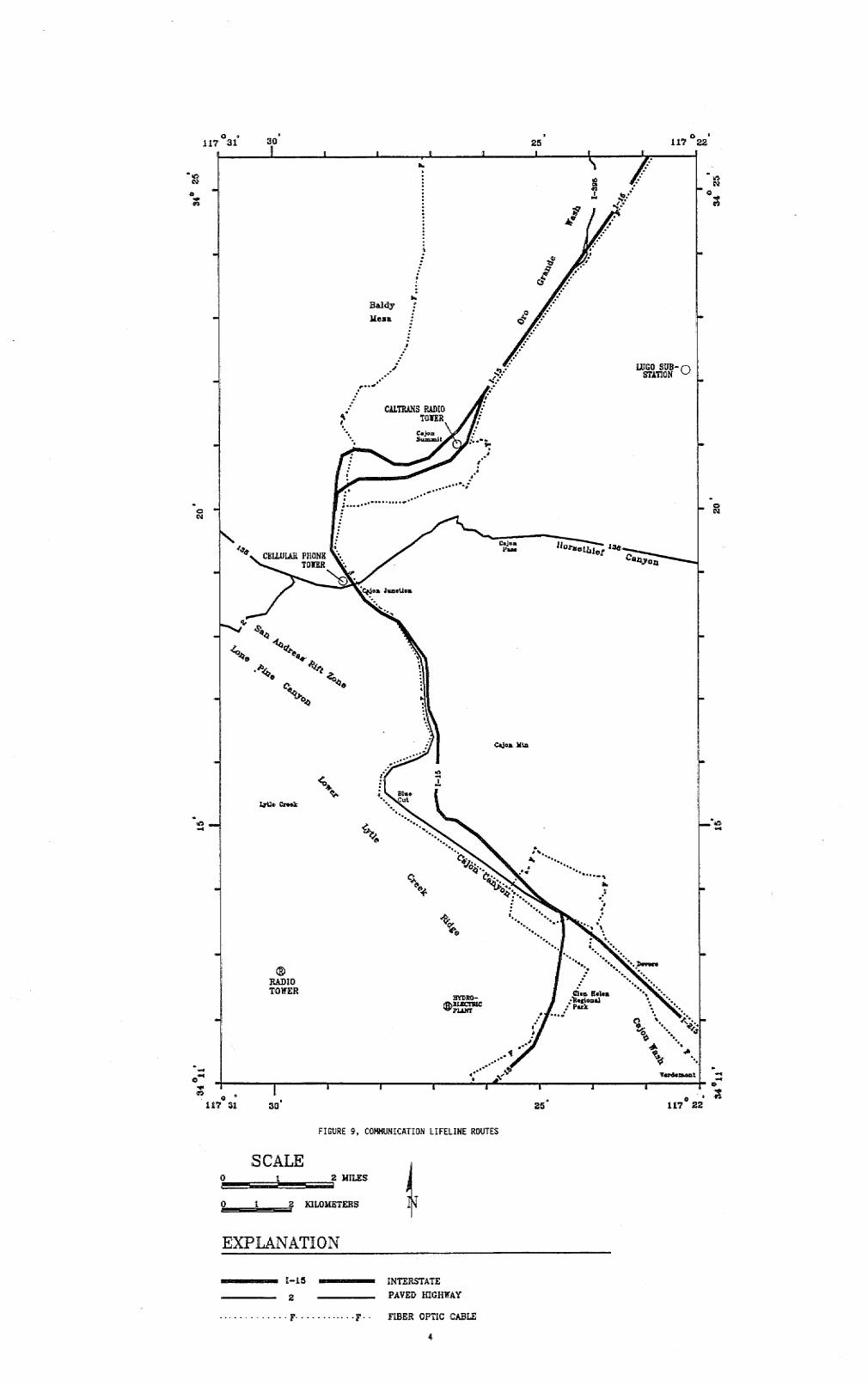
0l
C
*so ~ §° CElUUXk PilONE
j'%Sp<4°4~~~~~OI junu
94.. Q*-
C~~~~~~~~~~~~~~~~~~~C
e.cl~~~~~~~~I
RADIOTOWER
ftDRO-
n ~ ~ ~ ~ I
117 31 30
FIGURE 9, COMMUNICATION LIFELINE ROUTES
SCALEo 2 MILES
0 12 KILOMETERS
EXPLANATION
- -1J5 - INTERSTATE
2 _ PAVED IEaGHWAY
- * - - - -F..F FIBER OPTIC IaBLE
4
0 .
117 2225

~30 25,
FIGURE 16, ELECTRIC POWER LIFELINE ROUTES
2 MILES
K £OMETERs 44---15
I2
-- - - -
_____ v____ r-
INTERS5TATE
PAYED HIGIiWAY
POWER U1NES
BURIE AQUEDUCT
5
En
.0
0O
0 a'117 St
i;-
a.
117 2
SCALEI
EXPLANATION
7--

a ,117 22
117 22
FIGURE 20, FUEL PIPELINE LIFELINE ROUTES
- 1-15 -
2
- …--…----- -G ------ G--
INTERSTATE
PAVED EIGHWAY
PETROLEUM PRODUCT PIPEANES
NATURAL GAS PIPEIUNES
0 0 0 VALVES
B
117a317
0wo
0
a.117 31
0
SCALEI 2 MILES
0 1 2 KLOMETMES
EXPLANATION
-

0 .117 31
-4 _;1 4-
117 31 30
FIGURE 24. TRANSPORTATION LIFELINE ROUTES
SCALE2 MILTE1
0 I 2 aLOMIETERS 44EXP LANATION
_~ 1-15 - INTERSTATE
_ ~ 2 PAVED HIGHWAY
I -- +--- +I I - --I---4 - RAIMOAD
7
N
0
.' i
4;
CQ
.- ''.11
117 22