FEDERAL EMERGENCY MANAGEMENT AGENCY

Collocation Impacts on theVulnerability of Lifelines DuringEarthquakes with Applictions tothe Cajon Pass, California

Issued in Furtherance of the Decadefor Natural Disaster Reduction

Earthquake Hazard Reduction Series 61

FEMA 2261 February 1992

Collocation Impacts on theVulnerability of Lifelines During

Earthquakes with Applications to theCajon Pass, California

Submitted to the Federal Emergency Management AgencyWashington, D.C.

Submitted by:

INTECH Inc.11316 Rouen Dr.

Potomac, MD 20854-3126

Co-Principal Investigators:Dr. Phillip A. Lowe, INTEC, Inc.

Dr. Charles F. Scheffey, INTEC, Inc.Mr. Po Lam, Earth Mechanics, Inc.

COLLOCATION IMPACTS ON THE VULNERABILITY OF LIFELINES DURING

EARTHQUAKES WITH APPLICATION TO THE CAJON PASS, CALIFORNIA

TABLE OF CONTENTSVolume 1

ITEM PAGE

Table of Contents ..................... t .i

List of Figure............................................ ii

List of Tables........................................ v

1.0 CONCLUSIONS ................................... 1

2.0 INTRODUCTION ..................... . . 4

2.1 Background .. . ...... 4

2.2 Study Approach . . .................... . . 5

2.3 Chapter 2.0 Bibliography ................................ 6

3.0 SUMMARY .................................. . 6

4.0 ANALYSIS METHOD ...................................... 8

4.1 Data Acquisition . . . ............. 11

Lifeline and Geologic Information ... . . 11

Ground Shaking Intensity . . ............................... 13

Selection of the Earthquake Event ...................... 16

4.2 Calculation of Lifeline vulnerability .................. 16

Damage Assessment ................................... . 16

Shaking Damage .. . ..... 18

Fault Displacement. . . 23

Soil Movement . . ........................................ 24

Landslide .... 24

Liquefaction or Lateral Spread . . . .30

Highway and Railway Bridges . . ... 31

Times, to Restore the Lifeline to its Needed Service 37

Repair Time .............. 37

Access Time .... 38

Equipment and Material Time ........................... 39

4.3 Collocation Analysis .................................... 39

Impacts on Damage State....... .... 42

Impacts on Probability of Damage .... 42

Impacts on Time to Restore Lifeline Service . .43

4.4 Interpretation of the Results. .......................... 44

4.5 -Chapter 4.0 Bibliography ............................... 45

5.0 APPLICATION OF THE METHOD TO CAJON PASS ........ 47

5.1 Data Acquisition .... 47

5.2 Lifeline Collocation Vulnerability Analysis Results 55

Communication Lifelines .... 61

Electric Power Lifelines . . ............................ 6.8

Fuel Pipeline Lifelines ............................... 75

Transportation Lifelines .... 81

5.3 Chapter 5.0 Bibliography. . . 91

6.0 FUTURE STUDY NEEDS .... 91

Appendix A Modified Mercalli Intensity (MMI) Index Scale

i

LIST OF FIGURES

FIGURE PAGE

1 Flow Chart of the Analysis Method ....................

2 The "Attenuation Parameter k" for Use in CalculatingEarthquake Shaking Intensity .........................

3 Map of the U.S. Seismic Hazard Regions ................

4 Liquefaction Induced Damage ...........................

9

15

22

32

5 Map Showing the General Location of the CajonPass Study Area ....................................... 48

6 A Composite of the Lifeline Routes at Cajon Pass ...... 50

7 Identification of Collocations At Cajon Pass ... ....... 52

8 Lifeline Routes With Shaking Intensity andPotential Landslide and Liquefaction Areas ... ......... 54

9 Communication Lifeline Routes .......................... 62

10 Fiber Optic Conduits On A Bridge On The AbandonedPortion of Cajon Blvd. Extension ...................... 63

11 Details of the Fiber Optic Conduits of Figure 10 ...... 63

12 Fiber Optic Conduits On A Concrete CulvertThat Passes Under I-15 ................................ 64

13 Wall Support Details for the Fiber Optic ConduitsShown in Figure 12 .................................... 64

14 Surface Water Conditions Near The Toe of The I-15SRetaining Crib Wall ................................... 65

15 Fiber Optic Conduits Under a Heavy Water Pipe, Bothon a Highway Bridge ................................... 65

16 Electric Power Lifeline Routes ........................ 69

17 A Landslide Scar With Power Towers in the Slide Area .. 70

18 Power Lines, Natural Gas and Petroleum Products PipelinesIntersecting Over the San Andreas Fault Rift Zone ..... 71

ii

Figure

Figure

Figure

Figure

Figure

Figure

Figure

Figure

Figure

Figure

Figure

Figure

Figure

Figure

Figure

Figure

Figure

Figure

Figure 19 Power Tower at a Ravine Edge in the San Andreas FaultRift Zone .............. 72

Figure 20 Fuel Pipeline Lifeline Routes ...................... 76

Figure 21 Typical Long Open Span on the 36-Inch Natural

Gas Pipeline ...................................... 75

Figure 22 Two Natural Gas Pipelines Located Next to Highway 138 . 77

Figure 23 Natural Gas Pipeline Crossing Under Railroad Beds . 78

Figure 24 Transportation Lifeline Routes .......................... 83

Figure 25 I-15 Bridge Over Railroads in Cajon Wash .............. 84

Figure 26 I-15 Bridge Over Cajon Wash .................... ........ 84

Figure 27 Highway 138 Bridge Over I-15 .......................... 85

Figure 28 Railroad Bridges in Cajon Wash (I-15 Bridge in

Background) ................................... 86.... 8

Figure 29 Railroad Bridge Over Highway 138 (Collapse Expected) .. 86

Figure 30 Santa Fe Railroad Bubble Masonry Pier Bridge .8........ 87

Figure 31 Union Pacific Railroad Bridge With Power Lines

Overhead.....................................8....... 7

Figure 32 Typical I-15 Box Bridge Over the Railroads .90

Figure 33 I-15 and Access Road Bridges Over the SouthernPacific Railroad .............. 90..............I ...... 90

iii

LIST OF TABLESTABLE PAGE

Table 1. CAJON PASS IMPACTS OF LIFELINE PROXIMITY: EXPERTTECHNICAL ADVISORY GROUP .............................. 6

Table 2. ATC-13 DEFINITION OF LIFELINE DAMAGE STATE ... ......... 17

Table 3 SHAKING DAMAGE PROBABILITY MATRICES,ATC-13 Tables 7.10 .................................... 19

Table 4 MMI ADJUSTMENTS FOR SHAKING DAMAGE EVALUATIONS TO ACCOUNTFOR LOCAL CONDITIONS .................................. 23

Table 5 LIFELINE DAMAGE STATE FOR FAULT SURFACE DISPLACEMENTS,ATC-13 Table 8.9 ...................................... 24

Table 6 SOIL PARAMETERS FOR CALCULATING LANDSLIDE POTENTIAL ... 26

Table 7 LANDSLIDE SLOPE FAILURE PROBABILITY MATRICES,ATC-13 Table 8.7 ...................................... 27

Table 8 CONVERSION OF LANDSLIDE SLOPE FAILURE STATE TO DAMAGESTATE, ATC-13 Table 8.8 ................................ 29

Table 9 RELATIONSHIP BETWEEN LIQUEFACTION SEVERITY INDEX (LSI)AND DAMAGE STATE ...................................... 30

Table 10 PROBABILITY OF LIQUEFACTION GROUND FAILURE, PERCENT ... 31

Table 11 RELATIONSHIP OF BRIDGE VULNERABILITY INDEX TOBRIDGE DAMAGE STATE ................................... 33

Table 12 BRIDGE VULNERABILITY INDEX FOR EARTHQUAKE SHAKINGDAMAGE ................................................ 35

Table 13 ESTIMATED LIFELINE REPAIR TIMES TO 100% OPERATINGCAPACITY, ATC-13 Table 9.11 ........................... 38

Table 14 LIFELINE ZONES OF PHYSICAL INFLUENCE .................. 41

Table 15 MATRIX OF LIFELINE COLLOCATION AND INTERACTIONS ....... 56

iv

COLLOCATION IMPACTS ON THE VULNERABILITY OF LIFELINES DURING

EARTHQUAKES WITH APPLICATION TO THE CAJON PASS, CALIFORNIA

1.0 CONCLUSIONS

The purpose of this study was to:

develop a management screening tool that can be used bylifeline owners, designers and providers, operators, users,and regulators to sort through numerous collocation conditions

to identify the critical locations and to provide an estimateof the increased risk that results when such collocatedfacilities are subjected to an earthquake event; and to

analyze the Cajon Pass, California, situation to demonstratehow the screening tool can be used and to examine specificconditions at the Pass.

The resulting screening tool is an important development forseveral reasons:

1) it is the first documented method for examining multiplecollocation conditions and it is applicable to all lifeline

facilities. As improvements are made in the fundamental

analysis methods for individual lifelines or earthquakeconditions, they readily can be introduced into the screeningtool to improve its predictive ability;

2) its use can identify the most critical collocationconditions at a specific study area, thereby allowing limitedresources to be focused on the most important conditions forimproving the overall ability of the lifelines to survive anearthquake event;

3) its use can identify technical areas of uncertainty and/orpoor siting practices. This can identify the need for andlead to further research and studies to reduce the identifiedtechnical uncertainty or it can identify ways to mitigatesiting practices that are more vulnerable to inducingcollocation failure conditions; and

4) by being documented and made widely available by theFederal Emergency Management Agency, it is anticipated that itwill stimulate the earthquake and lifeline communities todeveloped improvements in the analysis method or even todevelop new, improved screening methods.

The development of the analysis methodology as well as, its testapplication to the Cajon Pass has highlighted several importantconclusions.

I

o Lifeline collocation can produce both benefits and increasedrisk of failure during earthquake events. A benefit ofclosely located transportation lifelines is that the secondlifeline can provide the detour or access route to the damagedsections of the first lifeline. However, intersectinglifelines generally result in the failure of one lifelineincreasing the risk of failure of the lifeline(s) it crosses.

o It is understandable that topographic conditions have led tothe routing of lifeline systems in corridors. However,manmade considerations that force the lifeline owners to usethe same rights-of-way for widely different lifelines (forexample, locating petroleum fuel pipeline and communicationconduits next to each other, routing natural gas pipelinesback and forth under a railroad bed, and having a mix oflifelines cross the earthquake fault zone at the samelocation) greatly increase the risk of failure for theindividual lifelines and the complications that will beencountered during site restoration after an earthquake.

o As compared to buildings, ground movement is more importantthat ground shaking for lifeline components, especially buriedlifelines and electrical transmission towers. This means thatmuch of the technical data base on earthquake shakingintensity is not critical for lifeline analysis, whereasimportant ground movement data and analyses are not as welldeveloped as the shaking intensity data. This suggests thatfuture studies need to emphasize obtaining ground movementinformation.

o A very useful screening tool has been developed during thisstudy. The tool can be used to identify the critical lifelinecollocation locations and the conditions that make themcritical. It can identify areas of technical uncertainty andpoor siting practices, and its use can identify importantresearch and development activities that can lead to loweredrisk of collocation-induced lifeline failures. It will be ofvalue to lifeline owners, designers and providers, operators,users, and regulators.

o The analysis tool has been successfully applied to the CajonPass, California. It has identified that for this semi-desertregion that:

The Cajon Junction, Lone Pine Canyon (which contains theSan Andreas fault zone), Blue Cut, and the area justsouth of the interchange between I-15 and I-215 are thecritical locations in terms of collocation impacts at theCajon Pass.

Fuel pipeline failures have the greatest impact on theother lifelines during the immediate recovery period

2

after an earthquake.

Current siting practices for fiber optic cables indicates

that more severe telephone communication failures than

have been experienced in past earthquakes can be

anticipated in future earthquakes when fiber optic

systems have become more dominant in providing the basic

telephone service.

Lifeline siting practices have not fully considered the

impacts that a new lifeline will have on existing

lifelines and, conversely, the impacts that the existing

lifelines will have on the new lifeline.

Transportation lifeline restoration of service is highly

dependent on sequentially repairing the lifeline damage

as the lifeline itself is needed to provide access to the

next damage location. Parallel repair operations are

more probable for the other lifeline systems.

Communication, electric power, and fuel pipeline

lifelines can generally be analyzed as a set of discrete

collocation points. The restoration of service at any

one point is not a strong function of the restoration

work that is needed at other collocation points. Thus,

if there is a restoration problem that will take a long

time compared to the other locations, it becomes the

"critical path" that sets the time period for the

restoration of the entire lifeline system.

When multiple lifelines of the same class are collocated

(such as installing all fiber optic cables or all fuel

pipelines in the same or parallel trenches) or when

multiple different lifelines intersect at a common point,

the reliability of each individual lifeline decreases to

the value of the "weakest link" of the combined lifeline

systems. In addition, repair times increase because of

local congestion and the concern that work on one

lifeline component could lead to damage of the other

different lifeline components.

o There is a need for further collocation lifeline studies: to

apply the newly developed screening tool to other locations to

assure that the methods can be transferred to other U.S.

locations and to analyze different lifelines, geographic, and

earthquake conditions; and to develop data and approaches that

can be used to further improve the predictive capabilities of

the screening tool.

3

2.0 INTRODUCTION

2.1 Background

Lifelines (e.g., systems and facilities that deliver energy andfuel and systems and facilities that provide key services such aswater and sewage, transportation, and communications are defined aslifelines) are presently being sited in "utility or transportationcorridors" to reduce their right-of-way environmental, aesthetic,and cost impacts on the communities that rely upon them. Theindividual lifelines are usually designed, constructed, andmodified throughout their service life. This results in differentstandards and siting criteria being applied to segments of the samelifeline, and also to different standards or siting criteria beingapplied to the separate lifelines systems within a single corridor.Presently, the siting review usually does not consider the impactof proximity or collocation of the lifelines on their individualrisk or vulnerability to natural or manmade hazards or disasters.This is either because the other lifelines have not yet beeninstalled or because such a consideration has not been identifiedas being an important factor for such an evaluation.

There have been cases when some lifeline collocations haveincreased the levels of damage experienced during an accident or anearthquake. For example, water line ruptures during earthquakeshave led to washouts which have caused foundation damage to nearbyfacilities. In southern California a railroad accident(transportation lifeline) led to the subsequent failure of acollocated fuel pipeline, and the resulting fire causedconsiderable property damage and loss of life. Loss of electricpower has restricted, and sometimes failed, the ability to providewater and sewer services or emergency fire fighting capabilities.

In response to these types of situations, the Federal EmergencyManagement Agency (FEMA) is examining the use of such corridors,and FEMA initiated this study to examine the impact of sitingmultiple lifeline systems in confined and at-risk areas.

The overall FEMA project goals are to develop managerial tools thatcan be used to increase the understanding of the lifeline systems'vulnerabilities and to help identify potential mitigationapproaches that could be used to reduce those vulnerabilities.Another program goal is to identify methods to enhance the transferof the resulting information to lifeline system providers,designers, builders, managers, operators, users, and regulators.

This report is the second of a series of three reports. The firstreport(' presented an inventory of the major lifeline systemslocated at Cajon Pass, California, and it summarized the earthquakeand geologic analysis tools available to identify and define the

* The numbers in superscript are references found at the end of eachchapter. 4

level of seismic risk to those lifelines. This report presents theanalytic methods developed to define the collocation impacts andthe resulting analyses of the seismic and geologic environmentalloads on the collocated lifelines in the Cajon Pass. The assumedearthquake event is similar to the 8.3 magnitude, San Andreasfault, Ft. Tejon earthquake of 1857. In this, report a new analysismethod is developed and applied to identify the increase in thevulnerability of the individual lifeline systems due to theirproximity to other lifelines in the Cajon Pass. A third reportspresents an executive summary of the study. The Cajon PassLifeline Inventory report and this present report taken togetherprovide a specific example of how the new analysis method can beapplied to a real lifeline corridor situation.

2.2 Study Approach

The approach used to develop the information for this report was asfollows. The Cajon Lifeline Inventory report('), additionalinformation provided during direct meetings with the lifelineowners, site reconnaissance surveys to validate the information andto examine specific site conditions of interest to the study, andexisting literature that describes lessons learned from actualearthquake events were compiled and thoroughly studied. Theprincipal investigators then hypothesized an analysis method thatcould be applied to the Cajon Pass lifelines to estimate theimpacts of proximity on their earthquake-induced performance andrepairs.

This analysis method emphasizes building upon existing data basesand analytic methods. In applications, it is recommended that theanalyses, studies, and information available from the lifelineowners be used whenever possible. In the event that sufficientdata on the lifeline response to earthquakes and the expected timeto restore the lifeline back to its, required service level are notavailable from the lifeline owners, the analytic methods, with someimportant modifications, of "Earthquake Damage Evaluation Data forCalifornial, ATC-13(3 ), are recommended as an appropriate alternativeanalysis method. In this project the "most probable restorationtime" was defined as the analysis parameter that best could be usedto define the impact of lifeline proximity on the individuallifeline's earthquake vulnerability.

The resulting method was then applied to the Cajon Pass lifelines.The U.S. Geologic Survey's digitized topographic map of the CajcnPass and the contiguous quadrangles were utilized. The commercial,computer aided, design program AutoCAD was used as it is readilyavailable to the public, thus the methodology is not limited tobeing dependent upon a specialized or proprietary computer program.With this tool, overlays of the lifeline routes with seismic andgeologic information presented in the inventory reportcl' were usedto identify the conditions and locations where the individuallifelines were most vulnerable to the hypothesized earthquake. The

5

analysis methods described in Section 4.0 of this report were thenapplied to the lifelines and the results are presented in Section5.0. Section 6.0 identifies future studies that could beundertaken to further qualify the analysis methods and to improvethe details of the specific analysis activities. Section 3.0provides a summary of the study.

As part of the study validation process, the draft results of thestudy were submitted to the project advisors, see Table 1, fortheir independent professional evaluation and to the lifelineowners and regulators who provided information for the preparationof the report or the Cajon Pass Inventory report. FEMA also sentdraft report copies to a select list of independent reviewers.Each comment received was addressed, and this final report then wasprepared and submitted to FEMA.

Table 1CAJON PASS IMPACTS OF LIFELINE PROXIMITY:

EXPERT TECHNICAL ADVISORY GROUP

William S. Bivins T.D. O'RourkeJames H. Gates Dennis K. OstromLe Val Lund Kenneth F. SullivanJohn D. (Jack) McNorgan

2.3 Chapter 2.0 Bibliography

1. P. Lowe, C. Scheffey, and P. Lam, "Inventory of Lifelines inthe Cajon Pass, California", ITI FEMA CP 120190, August 1991.

2. P. Lowe, C. Scheffey, and P. Lam, "Collocation Impacts onLifeline Earthquake Vulnerability at the Cajon Pass, -California, Executive Summary", ITI FEMA CP 050191-ES, August1991.

3. C. Rojahn and R. Sharpe, "Earthquake Damage Evaluation Datafor California", ATC-13, 1985.

3.0 SUMMARY

This report presents a systematic approach to calculate the impactsdue to the collocation or close proximity of one lifeline toanother during earthquake conditions. Specifically, thecollocation vulnerability impact is defined as the increase in themost probable time to restore the lifeline to its intended level ofservice. The analysis methods proposed are intended to be used inscreening analyses that determine which lifelines or lifelinesegments are most impacted by the collocation or close proximity ofother lifelines. Once the critical locations or conditions areknown, it may be equally important to reanalyze them using moredetailed analyses to further define the collocation impacts.

6

The methods proposed are to use the best available information todetermine the lifeline damage state, the probability that thedamage state or greater will occur, and the time to restore thelifeline to its intended service. Normally, such information isobtained from the lifeline owner/operator. However, a alternativemethod is proposed when such information is not available from thatsource.

The alternative method is based on building upon existingearthquake damage information and analysis methods which have been'compiled by the Applied Technology Council (ATC). In that manner,the analysis results can be compared with earlier or future studiesthat use the data base without the need to compare or justify thedata base. However, important improvements to the existing ATCdata base also are presented.

Collocation impacts, can be described in one of two broad terms: 1)the resource impacts (i.e., the increase in personnel, equipment,and material resources) that are required to return the totallifeline system to its needed operating capacity. This isperformed in the present method by summing the impacts at eachcomponent along the entire lifeline route. 2) the resource impactsat a specific location where multiple lifeline components arelocated. In both cases, the present method uses the most probabletime to restore the lifeline component or system to its neededoperating capacity as the appropriate measure of the resourceimpacts.

The analysis method has been applied to the lifeline systems in theCajon Pass, California, as a test case. It is clear that thecommunication, electric power, and fuel transmissions lifelinesystems that have the potential for collocation impacts are, ingeneral, not very sensitive to earthquake ground shaking forshaking intensities represented by Modified Mercalli Intensityindices of VIII or less (these are the values found at Cajon Passfor the assumed earthquake event). They are, however, verysensitive to ground movement expressed as fault displacement,landslides, or lateral spreads. Bridges are sensitive to bothground shaking and ground conditions (displacement, landslide,lateral spread, and local liquefactions at their foundationlocations).

It is understandable that topographic conditions have led to therouting of lifeline systems into corridors. However, manmadeconsiderations that force the lifeline owners to use the exact samerights-of-way for widely different needs (for example, locatingpetroleum fuel pipeline and communication conduits next to eachother, routing natural gas pipelines back and forth under arailroad bed, and having a mix of lifelines cross the earthquakefault zone at the same location) greatly increases the individuallifeline risks and the complications that will be encounteredduring site restoration after an earthquake.

7

The Cajon Pass example has identified that the communication,electric power transmission, and fuel pipeline lifelines generallycan be analyzed as a set of discrete collocation points. Therestoration of service at any one point is not a strong function ofthe restoration work that is needed at other collocation points.Thus, if there is a restoration problem that will take a long timecompared to the other locations, it becomes the "critical path"that sets the time period for the restoration of the entirelifeline system. Transportation lifeline collocation points,however, are sensitive to the damage that has occurred along theroute of the transportation system. That is, often it is necessaryfor the heavy equipment and material needed to have access to thedamage location by traveling along the highway or railroad itself.Thus, before access to a particular bridge can be made, it may benecessary to first repair all the damage sites on the route priorto that location.

4.0 ANALYSIS METHOD

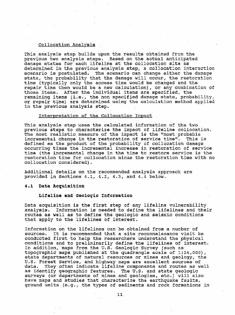
In performing an analysis of the impacts of collocation or closeproximity on lifeline systems and components for earthquake orother at-risk conditions, it is important that the most accuratedata and analyses be used to characterize the response of theindividual lifelines to the loads applied. Whatever method isapplied must be applicable to all the components within thelifeline system, because the evaluation of the collocation impactsrequires comparing the calculated time to restore the lifeline toits intended service for both the collocation and an assumed non-collocation condition. The general methods for performing such ananalysis are shown in the flow chart of Figure 1. If owner-supplied or site specific analysis methods are not available foruse in the detailed calculations, the following material (Sections4.1, 4.2, 4.3, and 4.4) can be used as the alternative analysismethod. This is discussed more fully in the following material.

Figure 1 shows a four step approach that can be used to analyze anylifeline under at-risk conditions (e.g., an natural or manmadedisaster condition). However, the present study only develops thedetailed information needed to analyze earthquake conditions. Thesteps are:

1) Data Acquisition;2) Calculation of Lifeline Vulnerability;3) Collocation Analysis; and4) Interpretation of the Collocation Impacts.

Briefly, these activities include:

Data Acquisition

This task is to assemble all of the information that defines thelifelines and their routes as well as the geologic and seismic

8

Figure 1, FLOW CHART OF THE ANALYSIS METHOD

FLOW CHART OF ACTIVITIES FORCALCULATING COLOCATION-INDUCED LIFELINE

VULNERABILITIES DURING EARTHQUAKES

RESULTMost probable Incrementalchange in restoration time

9

STEP 1DATA ACQUISITION

a Lifelines and routes

* Geologic and seismic conditions

* Colocation pointsa Lifeline analysis segments

STEP 2CALCULATION OF LIFELINE VULNERABILITIES

Assuming no colocation

& Damage state4 Probability of damagea Restoration time

STEP 3COLOCATION ANALYSIS

* Lifeline zones of Influence* Damage scenarioa Recalculate new

o Damage stateo Probability of damageo Restoration time

Il FSTEP 4

iMPACT OF COLOCATION- Incremental Change In restoration time

I Colocation damage probability

conditions that will place loads on the lifelines. Some analysisand organization of the resulting information is included in thisstep to facilitate the application of the analysis method to thespecific conditions of interest. Such analyses include identifyingthe collocation sites as well as dividing the lifelines intoconsistent sections for subsequent analysis.

Calculation of Lifeline Vulnerability

The geologic conditions identified during the data acquisition areused as input to a seismic analysis. Such data include thetopology of the area being studied, a description of the sedimentand rock structures, locations of water, and identification ofsurface ground slopes. Seismic conditions include identifying thelocation and type of the anticipated earthquake. These are used toestimate the earthquake shaking intensities (it is recommended thatModified Mercalli Intensity (MMI) indices be used to characterizethe shaking intensity) and earthquake-induced landslides and soilliquefaction locations.

During this analysis step, the earthquake intensities and groundmovements are use to determine the vulnerability of each lifelineat each collocation site as if it were the only lifeline at thatsite (e.g., as if there were no collocation there). Based on thedesign and placement of the lifeline component or segment and theseismic loads placed on it, the resulting damage state, probabilitythat the damage state will occur, and the time required to restorethe lifeline to its intended service can be calculated. Therestoration time is the sum of the time to repair the lifelineassuming all the equipment, material, and repair personnel areavailable at the damage location, plus the access time required totransport them to the damage location, plus the time required tohave them available to transport to the site.

If owner-supplied damage information is not available, it isrecommended that the analysis methods, as modified in this report,of "Earthquake Damage Evaluation Data for California", ATC-13,1985, (prepared by the Applied Technology Council of Redwood City,California) be used. When a study is to be performed for locationsoutside of California, professional judgement must be applied todetermine how to adjust, if at all, the data base of ATC-13. Themethods of "Seismic Vulnerability of Lifelines in the ConterminousUnited State, ATC-25, (presently in print at the Applied TechnologyCouncil, and identified as reference 20 in this report section) canbe considered for use. However, it is noted that the consistencyand validity of the ATC-25 approach has not been examined duringthe present study, and thus the methods of that study can not berecommended by the Principal Investigators of the present study.It is identified here for information only.

10

Collocation Analysis

This analysis step builds upon the results obtained from theprevious two analysis steps. Based on the actual anticipateddamage states for each lifeline at the collocation site asdetermined in the previous analysis steps a collocation interactionscenario is postulated. The scenario can change either the damagestate, the probability that the damage will occur, the restorationtime (typically only the access time would be changed and therepair time then would be a new calculation), or any combination ofthose items. After the individual items are specified, theremaining items (i.e., the non specified damage state, probability,or repair time) are determined using the calculation method appliedin the previous analysis step.

Interpretation of the Collocation Impact

This analysis step uses the calculated information of the twoprevious steps to characterize the impact of lifeline collocation.The most realistic measure of the impact is the "most probableincremental change in the restoration of service time"'. This isdefined as the product of the probability of collocation damageoccurring times the incremental increase in restoration of servicetime (the incremental change in the time to restore service is therestoration time for collocation minus the restoration time with nocollocation considered).

Additional details on the recommended analysis, approach areprovided in Sections 4.1, 4.2, 4.3, and 4.4 below.

4.1 Data Acquisition

Lifeline and Geologic Information

Data acquisition is the first step of any lifeline vulnerabilityanalysis. Information is needed to define the lifelines and theirroutes as well as to define the geologic and seismic conditionsthat apply to the lifelines of interest.

Information on the lifelines can be obtained from a number ofsources. It is recommended that a site reconnaissance visit beconducted first to help the researchers understand the physicalconditions and to preliminarily define the lifelines of interest.In addition, maps from the U.S. Geologic Survey (such astopographic maps, published at the quadrangle scale of 1:24,000),state departments of natural resources or mines and geology, theU.S. Forest Service, and highway maps are excellent sources ofdata. They often indicate lifeline components and routes as wellas identify geographic features. The U.S. and state geologicsurveys (or departments of mines and geologies etc.) will alsohave maps and studies that characterize the earthquake faults,ground units (e.g., the types of sediments and rock formations in

11

the areas of interest), landslide locations, water table data,etc.. State offices of emergency response (such as offices ofemergency preparedness or seismic safety offices), fire marshaloffices, state public utility commissions, water boards andcommissions, and the general professional literature on earthquakesare other important sources of information on lifelines and thepotential geologic/seismic conditions of interest.

The single most important source for lifeline information is theowner/operators. They will each have detailed route maps anddetails on their design, construction, and installation. However,as built drawings and construction information are frequentlydifferent than the "design" information. Thus, it is important todiscuss the information received with the suppliers, and tovalidate the understanding received with data from other sourcesand site reconnaissance visits.

Once the applicable lifeline data has been assembled, the lifelinecollocation or close proximity locations in the study region shouldbe identified and given a reference number. Also, each lifelineshould be divided into convenient segments that are reasonablyuniform in their characteristics. These activities are done to aidin the subsequent analysis steps. The application of the analysisalgorithms (to be described below) can be separately applied toeach lifeline collocation location, using the list of collocationlocation points as a check that all the needed locations wereconsidered, and using the lifeline segments to identify thephysical conditions at the collocation point being analyzed.

The lifeline segments or divisions selected for analysis should bereasonably "uniform" in that the lifeline components should besimilar within the segment, the shaking intensity (as measured bythe Modified Mercalli Intensity (MMI)) index should be similar, theground conditions should be similar (that is, areas of groundmovement should be analyzed separately from areas of stableground), and access for repair crews, equipment, and material tothe lifeline proximity points along the segment should bereasonably the same. With this approach, lifelines, such as buriedpipelines or electrical transmission lines, can be divided intolong segments. Their division is primarily set by the groundconditions and the MMI values. Other lifeline systems that havefrequent component changes in them, such as transportation systemsthat include bridges separated by roadbeds, need to be separated bycomponent and access route, and sometimes the roadbed must befurther divided to account for ground condition or MMI changes.

Whenever possible, standard measures of earthquake events should beused to characterize the seismic conditions in the study area. Inthis way the results of the study more readily can be compared withother published data, which allows the conclusions to be validatedby such other available information. Thus, earthquake magnitude orthe earthquake "size" can be represented by the Richter scale.

12

Ground Shaking Intensity

Several methods to characterize the intensity of the shaking of anearthquake were considered. Items considered included themagnitude and extent of the shaking. Although ground acceleration,velocity, and displacement are more appropriate for evaluatingspecific lifeline designs, the use of intensity scales are moredominant in the literature. Rossi-Forell (RF) and ModifiedMercalli Intensity (MMI) scales are commonly used as a measure ofintensity. MMI is recommended for use since it is more widely usedin the earthquake literature, although it is a subjective scalethat is dependent on individual interpretation of its meaning.Appendix A presents the detailed definitions of MMI..

The MMI scale includes 12 categories of ground motion intensityfrom level I (not felt) to level XII (total damage). The use ofRoman numerals was done to discourage analysts from trying toconsider half scale values. This further implies that the MMI is abroad measure of the shaking intensity. The individual MMI scalesare almost exclusively characterized in terms of building damage,so their usefulness for modern lifeline structures and componentsis somewhat restricted. ATC-l3 (2, provides a detailed estimate oflifeline damage probability as a function of the MMI scale. As anexample of potential interpretation problems, the MMI scale IXidentifies that "runderground pipes are sometimes broken" while ATC-13 for MMI = IX estimates in California that pipe breaks will occurwith a total probability of 91.3%. This illustrates the subjectivenature of the MMI scale. Nevertheless, it is commonly used tocharacterize earthquake intensity, *and for consistency itrecommended as the proper characterization parameter for examiningthe collocation impacts on lifeline vulnerability to earthquakes.

Although there are two computer models,(3,4 ,5) that calculateearthquake intensit and that are applicable to the conterminousU.S., the Evernden ) model is recommended because it has beenverified by comparison with historical earthquakes, it incorporatesthe local sediment conditions and such sediment conditions aregenerally available in the national U.S. Geological Survey geologicdata base and in the data bases of the various state offices ofmines and geology or natural resources, it is easy to use, it isreadily available to researchers, lifeline owners, and to otherswho may need to apply the methods of this study to other regions inthe U.S., and it facilitates comparisons of this research with thatof others 7) who have used the Evernden Model. The Advisors to thisProject were concerned that the Evernden model may not be asaccurate near the earthquake fault location (it appears tounderestimate the EMI values there) as it is in predicting the farfield effects. Discussions with the staff of the CaliforniaDivision of Mines and Geology confirmed that they had similarconcerns. The recommended solution is to increase the calculatedMMI value by one scale level at locations near the earthquake faultzone. For most lifeline components this is expected to have a

13

small impact, because the fault displacement effects there areexpected to overshadow the shaking effects represented by theincreased MMI value.

The Evernden model has been coded in a computer program, QUAK2NW3.Appropriate input data files are available with the model, and theywere verified for use in the present study. They include:

(1) a fault data file that identifies the location of thegeologic fault by a series of uniform point sources.They can be spaced as closely as desirable.

(2) a ground condition file that identifies the soilconditions (soil and ground geologic units ordescriptions). The spacing of these ground unitsprovides the calculation grid for the program. Everndentypically organizes the ground condition into 0.5 minutelatitude by 0.5 minute longitude grids, and they wereused for the present study.

(3) a pseudodepth term "C" which is chosen to give the propernear-field die-off of the shaking intensities. Everndenhas previously analyzed earthquakes along the San Andreasfault, and his value of C (10 kilometers) was used inthis study. Values for other faults can be selected withconsultation with Dr. Evernden or by professionaljudgement.

(4) an attenuation parameter "k" which controls the rate ofdie-off of peak acceleration as a function of distancefrom the fault being analyzed. Evernden has identified avalue for coastal California, eastern California and theMountain States, the Gulf and Atlantic Coastal plains,and the rest of the eastern U.S., and these values areshown in Figure 2. The coastal California value was usedin this study, k = 1.75.

With the above input, QUAK2NW3 computes the acceleration associatedwith the energy release along each position of the fault.Earthquake intensities are calculated in terms of the Rossi Forellscale, and then the MMI value is computed from a correlation thatEvernden developed for that purpose. The intensity is firstcomputed for a reference ground unit condition (e.g., saturatedalluvium), and then the intensity value at each grid point isadjusted for the actual ground condition specified in the groundcondition file. The output of QUAK2NW3 can be used as input into adigital plotting program, so that the regions of uniform MMI indexcan be automatically plotted over the routes of each lifelinesystem studied. In the present study the commercially availableprogram "AutoCAD" was used, although other similar programs wouldbe just as appropriate. An important criteria for the selection ofthe plotting program is that it should be able to read the

14

Figure 2, THE "ATTENUATION PARAMETER k" FOR USEEARTHQUAKE SHAKING INTENSITY

IN CALCULATING

APPROXIMATE PATTERN OF ATTENUATION CHARACTERISTICS (k-VALUE DISTRIBUTION)THROUGHOUT THE CONTERMINOUS UNITED STATES

15

ditigitized files of the U.S. Geological Survey topographic maps.Those maps include the routes of many of the lifelines and thegeographic elevation contours. Later when ground slopes are neededto calculate landslide and liquefaction potential, the computerprogram can be used to automatically perform the calculations.Thus, a single program can conveniently incorporate and graphicallypresent all the key data: lifeline location, fault traces, MMIvalues, and ground slopes.

Selection of the Earthquake Event

The next step is to identify the earthquake event for the analysis.Based on the faults in or near the study region, the QUAK2NW3program can be used to perform a sensitivity evaluation to identifythe appropriate earthquake event. All that is required is to inputvarious earthquake events (length and location of the faultmovement, the ground conditions, the depth of the earthquake, andthe attenuation parameter). The results of several analyses canthen be compared to identify the most realistic event for theanalysis. Key additional data that should be considered is theprediction of the magnitude and the probability that an earthquakewill occur near or in the study region. Such predictions areavailable from Federal and state seismologic offices.

4.2 Calculation of Lifeline Vulnerability-

Again, it is recommended that the lifeline owners/operators beconsulted to determine if they already have detailed calculationson their lifeline's vulnerability to earthquake events. If so,that approach may be the most detailed available. As analternative, the following sections identify how the ATC-13information, with important modifications, should specifically beused if such owner/operator information is not available.

Damage Assessment

To determine the potential damage state that occurs, the impacts ofshaking, fault displacement, and soil movement due to eitherlandslide or liquefaction conditions have to be considered. Thetotal damage state is the sum of these individual components;however, if one of these components dominates the others it can beused without adding the other damage states (this is often theactual situation). However, when that is done a similar approachmust be used for both the analysis performed while assuming nocollocation impacts and for the analysis performed while assumingcollocation impacts. Also, adding the separate damage states mayover estimate the total damage state. Knowledge of the physicalsituation and professional judgement must be applied to determinethe realistic total damage state.

There are seven categories of damage state defined in ATC-13. Theyare shown in Table 2.

16

Table 2ATC-13 DEFINITION OF LIFELINE DAMAGE STATE

Lifeline For Non Pipeline For PipelineDamage State Lifelines LifelinesNo. Description % Damage Breaks/kilometer % Damage1 - None 0 0 02 - Slight 0.5 0.25 0.63 - Light 5 0.75 24 - Moderate 20 5.5 145 - Heavy 45 15 3.86 - Major 80 30 757 - Destroyed 100 40 100

In the present method, the important parameter is theidentification of the Damage State Number, a number from 1 to 7.Thus, percent damage or breaks per kilometer are not the neededvariable. The experts that developed ATC-13 used the followingdefinitions for damage state: percent damage meant the estimate ofthe dollar value of the earthquake damage divided by the dollarcost to replace the entire lifeline. However, for pipelines theywere asked to think in terms of breaks in a pipeline per kilometerof pipeline length. Within a kilometer segment, 15 breaks mayactually cost the same as 40, since the expected procedure would beto simply replace the entire kilometer length rather than to makesuch a large number of individual repairs and still be concernedthat an additional partial break was undiscovered and thus remainedunrepaired. Similarly, an electrical transmission tower with 45%physical damage would probably be replaced entirely, as it wouldnot be worth the risk to the owner to make such extensive repairswhen a new tower may be less expensive to install and certainlywould be more reliable in the future. Thus, when the ATC-13definition is applied to a large number of similar lifelinecomponents, then, on the average, the damage state may properlypredict the condition of the sum of the individual repair costsdivided by the total replacement costs for all the components.

However, in the present analysis method, the ATC-13 data will beapplied to individual lifeline components. It is acceptable to usethe data in this. manner as it provides an expert knowledge base forestimating the damage state, and the final result of interest inthe present analysis method is not the damage state but a time torestore lifeline service. Its use for single lifeline componentswould be less accurate if the desired result were the percentdamage to be used to calculate a cost of repair (that is, ATC-13 ismore accurate for costs averaged over a large number of cases thanit would be for a single case). The proposed analysis methodcould, however, be improved if -a new expert opinion study of thedamage state and probability for that damage state for singlelifeline components were to become available.

The following material indicates how the data of ATC-13 are

17

proposed for use in evaluating the collocation impacts of lifelinesduring earthquake events.

Shaking Damage

The shaking impact of the earthquake event can be estimated byusing Table 7.10 (pages 198-217) of ATC-13. For convenience, themore frequently needed tables for lifeline analysis are reproducedin this report as Table 3.

These tables present the collective judgement of the probabilitythat a class of lifeline components will incur a given damage statelevel, as a function of the Modified Mercalli Intensity (MMI)index. They were developed by using a modified Delphi method thatemployed a large number of experts who provided their opinion as towhat was the probability that a damage level would be experiencedfor a given imposed value of shaking intensity, MMI.

The trend in the probability data would normally be expected toshow that, as the MMI increases, more of the lifeline componentswould be expected to experience higher damage states. Thus, forincreasing values of MMI, the shape of the probability curve shouldbe expected to have its peak value move towards higher damagestates and the magnitude of the peak value decrease as the width ofthe probability curve increases. However, at MMI = XII theprobability curve should again focus over the narrow band of damagestates 6 and 7. The information for bridges, highways, and buriedpipelines and conduits follow this pattern. It is less evident forelectrical transmission towers and railroads. The methodology forcalculating shaking damage collocation impacts, because it is basedon the ATC-13 data, will be less accurate for electricaltransmission towers and railroads, compared to buried pipeline andconduits, highways, and bridges. Still, the PrincipalInvestigators and Advisors for this project judged that the datawas adequate for the analysis purposes proposed in this report.

In Table 3 the lifeline items are: Facility Class 24-multiplesingle span bridges; Facility Class 25-continuous/monolithicbridges; Facility Class 31-underground pipelines; Facility Class47-railroads; Facility Class 48-highways; Facility Class 55-electrical towers less than 100 feet high; and Facility Class 56-electrical towers more than 100 feet high.

In this report the ATC-13 shaking damage data is used in thefollowing manner. For the lifeline component or segment beingconsidered, the appropriate table is entered using the MMI value atthe collocation'being analyzed. The table is entered to identifythe greatest probability value in the column under the MMI listing.In the sample below enter the table (on page 21) for MMI = VIII.Reading to the left of that maximum probability, the most probabledamage state is then read from the left most column.

18

Table 3SHAKING DAMAGE PROBABILITY MATRICES, ATC-13 Tables 7.10

Damage Probability Matrices Based on Expert Opinion forEarthquake Engineering Facility Classes

DamageState

Modified Mereaili IntensityMultiple Single Span Bridges

vYI VIi I III [S II XIII

1 3.0 iii fit Itt iii nj it

2 57.0 12.3 in i} in IF tiF3 i1i 85.7 70., fi t ri ii iti4 - fi i 29.1 71.1 iffi iM5 it Mi i 28.9 82.4 *ti t ii

6 iiit t1i i-n 1H.9 100.0 int7 i i ii off ii t 100.0

Continuous/Monolithic Bridges

v] V II VIII II I II III

1 93.6 8. 1 0.9 i ii itn ii2 6.4 77.8 17.6 itt it ii tt3 it 14.1 78.6 56.5 it i ifn

4 tit tt 2.9 43.5 1.9 1.2 0.75 i.E.! ii iii it 98.2 36.8 5.7

6 fiti i tit fit in 61.9 39.17 ti iii iti tit tin 0.1 54.5

lUnderground Pipelines and Conduits

VI VII VIII II I II XII

1 100.0 9.a, 20.9 8.7 tlIt ti it:2 it 0. 2 54.1 34.2 1.3 tit tlit3 itn a:: 17.2 36.1 7.9 os5 i1t4 it: t11 7.8 21.9 ;89.5 64.5 4.55 tit tit t1t 2t1 1.1 29.6 56.46 Itt tit t1t it: 0.2 3.3 37.97 ilI sit iI in Iti 0.1 1.2

***Very small probability

19

Table 3 (Continued)SHAKING DAMAGE PROBABILITY MATRICES, ATC-13 Tables 7.10

Modified Mercalli Intensity

Railr

VI ViI Vill

9.855.434.9

oft,

it#

0.112.387.00.6offoffit

-oads -

II I I1 III

M

0.373.925.8

off"I

',0

35.564.10.4off

MI

fit

10.280.89.0Hit

I..

III

tI

0.425.567.96.2tt

VI Yll

Highways

Vill ll

3.36.7

ftt

It

HIII

18.961.519.7tt

ftIII

2.927.068.8

1.4ittoffIII

Electrical Towers

VI VIl Vlll

94.15.9fittt

MHt

itt

6.978.814.3Ittott

.i.f

1.051.048.0itItt

HtIMI

Electrical Towers

VI VII Vll

93.66.4off

off

fit

it

itI

7.372.120.6

ttt

off

tII

itt

1.850.947.3

off

HfiII

Mt

1.0-13.875.49.8

Ht

Less

II

#iI

2.996.3

0.8If

*I

#it

it

1.359.039.10.6H

lt

Than 100 Feet High

I

63.736.3

MI

fiI

MI

More Than 100

1X I

III

7.592.20.3III

It*

it

oft

0.372.527.2iIIfitft

II Ill

itI

10.682.76.7itI

Feet

11

Ftt

16.679.44.0H

it§

***Very small probability

DamageState

1234567

94.15.9III

H,

tttHI Ht

1234567

I II XII

ilI

0.120.565.214.2

ft

itI

4.650.243.4

1.8off

1234567

1234567

III

0.539.059.21.3

High

Ill

III

0.838.25B.82.2i.

20

Sample ATC-13 Shaking Damage Matrix

Damage State Modified Mercalli Intensity IndexVI VII VIII IX X XI XII

1 100 99.8 20.9 8.7 - - -

2 - .2 54.1 34.7 1.3 - -

3 - - 17.2 36.1 7.9 .5 -4 - - 7.8 21.9 89.5 66.5 4.55 - - - - 1.1 29.6 56.46 - - - - .2 3.3 37.97 - - - - - .1 1.2

For a EMI = VIII, the largest probability is 54.1 (identified inbold); therefore the assumed damage state is damage state 2 (alsoin bold). The probability that the damage state or greater willoccur is the sum of its probability and all the probabilities forlarger damage at the MMI value of interest: (54.1 + 17.2 + 7.8) =

79.1%, or 79% for use in the subsequent analyses.

The data represented in Table 3 was developed based on assuming thefacility construction methods were in California. Since Californiahas incorporated seismic design criteria in some of their codes andstandards, it raises a question as to how the data should beapplied to other U.S. regions. The most direct approach would beto consider the design and construction practices at the study areain question, and to adjust the damage state predicted by Table 3 toaccount for differences with respect to California.

Rojahn 2 03 has developed a different approach. He suggests that theEMI value can be adjusted to account for the different design andconstruction practices. Increasing the MMI value would imply thatthe local practices are less conservative for earthquakeconsiderations than those used in California. Decreasing the XMIvalue would imply the opposite. Figure 3 shows the U.S. dividedinto seismic hazard regions. The Rojahn adjustments for arepresented in Table 4. He has used Figure 3 to divide the U.S. intofive broad regions: California region 7; Other U.S. areas, of region7; California regions 3 to 6; Puget Sound region 5; and all otherU.S. regions.

Table 4 is provided for information purposes. Data for additionallifeline components are provided in reference 20. Rojahn did notjustify the selection of the Table 4 values or explain whyadjustments are needed for California (recall that ATC-13 was basedon assuming that it applied to California). One of the importantrecommended follow-on studies to the present work is to apply thepresent screening tool to another U.S. location. One purpose ofsuch a study would be to examine the validity of the adjustments toMMI recommended by Rojahn.

21

Figure 3, MAP OF U.S. SEISMIC HAZARD REGIONS

NEHRP Seismic Map Areas OTC, 1978; BSSC, 1988).

Seismic RiskRegions

6 71 6

g S4

3

2

U1

22

Table 4EMI ADJUSTMENT FOR SHAKING DAMAGE EVALUATION

TO ACCOUNT FOR LOCAL CONDITIONS(the region numbers correspond to the numbers of Figure 3)

RegionCalifornia, #7Other area, #7California, #3-6Puget Sound, #5Other U.S. regions

Multiple Span Continuous Rail beds &Bridges Bridges Hichways

0 0 0I103

111

2 or 3

0000

Region and NumberCalifornia, #7Other area, #7California, #3-6Puget Sound, #5Other U.S. regions

RailroadBridges

-10

-101

Water Trunk Water PipeLines Distribution

O 10 10 10 11 2

Region and NumberCalifornia, #7Other area, #7California, #3-6Puget Sound, #5Other U.S. regions

Region and NumberCalifornia, #7Other area, #7California, #3-6Puget Sound, #5Other U.S. regions

Electrical ElectricalTowers Over Towers Less than100 ft. high 100 ft. high

0 'o 0

o 0Of 0

'0 1

Natural Gas Natural Gas OilTransmission Distribution Pipelines

-1 '0 -1-l-l-1

0011

-1-1-1-1

Fault Displacement

In ATC-13, the maximum fault surface displacement, D, in meters iscalculated from the equation:

Log D = -4.865 + 0.1719 x M; where M is the earthquakemagnitude

ATC-13 identifies that the fault average displacement is typically77% of the maximum, and that 30% of the maximum displacement on themain fault is characteristic of the displacement on subsidiaryfaults.

The damage states for the estimated displacement are obtained from

23

ATC-13 Table 8.9 and are presented in Table 5.

Table 5LIFELINE DAMAGE STATE FOR FAULT SURFACE DISPLACEMENTS,

ATC-13 Table 8.9

Facility Type Damage State (% damage is given in the parentheses)and Location For Various Values of Displacement in meters

Displacement = 0.2 m 0.6 m 1 m 3.5 m 10 mSubsurface StructureIn Fault Zone 5(50) 6(80) 7(100) 7(100) 7(100)In Drag Zone 4(20) 5(40) 5(60) 6(80) 7(100)

Surface StructuresIn Fault Zone 3(10) 4(30) 6(70) 7(100) 7(100)In Drag Zone 0(0) 0(°) 3(2) 3(10) 4(20)

The "Fault Zone" is defined as being within 100 meters of the faulttrace, the "Drag Zone" is defined as being within 100 to 200 metersof the fault trace. If lifeline components are judged to havefailed because of fault displacement, then the collocation impactwould be only an increase in the time to restore the lifeline toits needed level of operation (e.g., damage greater thancatastrophic is not meaningful). Such time increases would beattributed to the construction activity and the need to assure thatconstruction on one lifeline does not lead to damage onreconstructed other lifelines.

Soil Movement

Many texts separately define the impacts due to landslides andlateral spread (or liquefaction). However, they may be thought ofas being part of a continuum of soil movement with the slope of thetopography being a parameter that identifies whether the movementshould be calculated as a landslide or a lateral spread (orliquefaction). That is the approach proposed in the presentanalysis method.

Landslide (landslides occur on slopes greaterthan 50)

It is proposed that the historical landslides in the study area beidentified and considered as potential landslide req ions when thecollocation evaluation is made. Keefer and Wilsonsi0) and Sadlerand Morton" 1 ') have identified that landslides are associated withmany historical earthquakes and that shaking is one of the maintriggering agents for landslides. Actual site reconnaissancevisits are recommended as a means to verify the location ofhistorical landslides for any area being studied. In the presentstudy, a comparison of the known slides with the geologic unit mapidentified that many of the landslides were associated with areas

24

where Pelona Schist is the bedrock unit. Other researchers areadvised to examine the geologic sediments and rocks in the areaswhere they intend to evaluate collocation and to be sensitive tothe location of Pelona Schist.

It is proposed that the method of Legg et. al. CY2 ) be used toidentify additional areas where landslides may occur. It is basedon the sliding block model proposed by Newmark 1 3 ); Wilson &

Keeferc'4) have proposed a similar model.. However, the Wilson andReefer model requires using recorded accelerograms or predictionsof ground acceleration while the Legg method is related to usingMMI. The Legg model is the method used in ATC-13 to define thedamage state and probability of damage for landslides. Also, itwill be easier to apply the Legg model to other regions in theU.S.. Because of these items, the Legg method was adopted forpredicting additional landslide areas.

The Legg method consists of the following basic steps:

Step I Solve for the "critical acceleration" of the slopefor a given combination of slope angle and soilproperties. A formula derived from the stabilitysolution of an infinite slope was used by Legg andalso by Wilson and Reefer, and it is provided below.

Step 2 Use the critical acceleration to enter a table of"slope failure state"' versus DMI value. The tablevalues identify the potential for the slope to moveas a landslide. The tables are provided as Table8.7 of ATC-13 and are reproduced below as Table 7.

Step 3 The slope state is related to damage state in Table8.8 of ATC-13, which is presented below as Table 8.However, the ATC-13 Table 8.8 has been extended tomore accurately account for buried lifelines, basedupon expert opinion obtained during the presentstudy.

The formula for the critical acceleration is given by:

ar/g = c/(yh) + cos e tan ¢ - sin 0 ; where

a= the critical acceleration, ft/sec2

g = the gravitational constant, 32.2 ft/sec2

c = the effective soil cohesion factor, lb/ft2

= the soil density, typically 100 lb/ft3

h = the thickness of the soil block, typically 10 ftl = the slope angle, degrees

= the angle of friction of the slope material,degrees

Note, this equation applies to dry slopes.

25

The soil parameters recommended for use are given in Table 6.

Table 6SOIL PARAMETERS FOR CALCULATING LANDSLIDE POTENTIAL

Shear Strength ParametersGeologic Unit Cohesion. c (Vfs) Friction Angle, (degree)

Paleozoic Rocks 300 35Older Cenozoic Rocks 0 35Older Alluvium 0 30Young Alluvium at ShallowGround Water & Pelona Schist 0 20

Wilson and Keefer (14 have also developed an analysis for saturatedand dry slopes. They use a 35 degree friction angle for sands,sandstones, and crystalline rocks, and 20 degrees for clayey soilsand shales. They present a graph of the critical acceleration as:

0.5 - -_ _ _ _ _ _ _ _

Z Plots of critical acceleration (Ad) versus slope steepness0

for three sets of lithologies: group A, strongly cemented rocksG% \ \ \ \(crystalline rock and well-cemented sandstone); group B, weakly

uj 0.3 ) v \ \ X \ cscemented rocks (sandy soil and poorly cemented sandstone); groupU \ \ O~y&> 9 96\ C, argillaceous rocks (clayey soil and shale). The cohesion factor,< 0 S C- 0 c'I'yh, for group A assumes values of c'-=300 psf. -y = 100 pcf. andX God O'er \S\ h -10ft. The angle of internal friction (e ) (peak strength, undrainedU \ '0< ,\ \ O \ 0 conditions) is 35° for sands, sandstone, and crystalline rocks and

I \\ \ 200 for clayey soils and shales. The solid lines depict dry slope_0_1 | materials, and the dashed lines depict saturation from the slide

plane to the surface.

10¢ 20' 300 i 400 5005% 15% 30% 50% 70% 100%

SLOPE

Either the Legg formula or the Wilson graph is acceptable fordetermining the critical acceleration, it's numeric value will beused in the Legg tables discussed below.

The appropriate soil parameters from Table 6 or other referencesshould be identified. The formula or graph is then used todetermine the value of the critical acceleration, which in turndetermines the slope stability (unstable, low, moderate, high,stable, very stable) so that the ATC-13 Table 8.7 (Table 7 givenbelow) can be used to define the state of slope failure (Table 7uses the Legg definitions for terms of slope failure state andslope stability scale, and those definitions also are provided withthe table).

26

Table 7

LANDSLIDE SLOPE FAILURE PROBABILITY MATRICES, ATC-13 Table 8.7

Sope Fitflue Probabfity ¶abieft(Summer Conditico)

SLOPE SrABIErrY: UNSTABLE, .4 c .01 r

SLOPE YMIFAILURESTATE VI VD vm TX x Xl Xly

LUG&T 0 0 0 a 0 0 0

MODERATE a 0 a a a 0 0

HEAVY f00 50 40 30 20 5 a

SEVERI S0 40 45 50 55 60 S5

CATASTROPHIC l 1a i5 20 i5 15 50

½ 10I% 100% 100% 30% 100% 100% 2100%

LOnPE SriBLMrs LOW, .01 a , 0 c

SLOPE MMIYADLUR!STATE VI Vy Y3 ix X XI XE

LIGHT 40 25 15 10 5 0 0

iODERAIE 50 30 35 l0 20 10 0 O

HEAVY 25 35 40 40 35 35 30

SEVERC 5 10 10 15 20 35 40

CATASTROPHIC 0 0 a 5 10 20 30

½ 1 t00 100% 300% I00% 100% 100% 100%

SLOPE STABSLTYi XODIXATE, 0.1 a, -3 E

SLOPE MMIFhALURESTATE VI VI VM TX x xi

LIGHT 100 100 15 1 55 20 0

MODERATE O a 10 20 25 Jo 10

HEAVY 0 0 5 la 15 25 40

SEVERE 0 0 0 0 5 i5 20

CATASTROPHIC a a 0 0 0 10 10

Zp 100% l10 100% 100% 100% 300% l0

SLOPE STABEJrYza MIR, 0.3 p < a, c 0.5 r

SLOPEFAILUR ESTATE Vi VE vm rX X xi xEl

LIGHT 100 100 100 95 &5 !0 s0

MODERATE 0 0D 0 5 II 15 20

HEAVY 0 0 0 0 5 5 15

SEVERE C, o 0 0

CATASTROPH 0 a o0 0 0 0 0

Zp 100% 300%. 10a 100% 100% 1005S 10%

SLOPE SABUI STAEL., 0.5 c %( 0.7

SLOZ MMRFAGERFAILURESTATE VI vu vY 1x x X1 XII

LIGHT 10O 100 100 100 00 Is 75

MODERATE 0 0 0 0 10 l0 15

HEAVY 0 0 0 0 C 5 la0

SEVERE 0 0 0 0 0 0 C

CATASTROPHIC C 0 0 0 0 0 0

: D100%. 10096 I00 I00% 100% 100% 10C%

SIAPE sTABIlfrft Y=V 1TA l 0.1 E < 4e

SLOPE MMI

STATE V yn a TX X n XE

LIGHT 100 100 100 100 100 t SO

iAODERATE 0 0 0 0 0 1 15

HEAVY I 0 0 0 0 0 5

SEVERE 0 0 0 0 0 0 1

CATASTROPHIC 0 0 0 0 0 a 0

, 100 100 10100 %00% 100% 100% 100%

27

Table 7 (Continued)Definitions

SLOPE FAILURE STATE SCALE

LIGHT- Insignificant groundmovement, no apparentpotential forlandslide failure,ground shaking effectonly. Predicteddisplacement lessthan 0.5 cm.

MODERATE- Moderate groundfailure, small crackslikely to form,cracks similar tohaving a lurchphenomena. Predicteddisplacement 0.5 to5.0 cm.

HEAVY- Major ground failure,moderate cracks andlandslidedisplacements witheffects similar toliquefaction orlateral spread.Predicteddisplacement 5.0 to50 cm.

SEVERE- Extreme groundfailure, large cracksand landslidedisplacements witheffects similar tolarge-scale faultdisplacement.Predicteddisplacement 50 to500 cm.

RELATIVE SEISMIC SLOPESTABILITY SCALE

V - Very stable, not likely tomove under severe shaking,ac 2 0.7g.

S - Stable, may undergo slightmovement under severeshaking, 0.5g < a < 0.7g.

H - High, may undergo moderatemovement under severeshaking, some landslidesrelated to steep slopes,saturated conditions, andadverse dips, 0.3g < ac <0.5g.

M - Moderate, may undergomajor movement undersevere shaking or moderatemovement under moderateshaking, numerouslandslides, rock fallsabundant, unconsolidatedmaterial deforms andfails, 0.lg < ac < 0.3g.

L - Low, may undergo majormovement under moderateshaking, abundantlandslides of all types,0.0lg 5 ac < 0.1g.

U - Unstable, may undergomajor movement underslight shaking, most ofthe area and/or materialfalls, ac < 0.01g.

cm = centimeterCATASTROPHIC- Total ground g = gravitational constant

failure, withpredicteddisplacement greater :than 500 cm.

28

To use Table 7, it is necessary to enter it with the criticalacceleration, ac, and the MMI value. The critical accelerationvalue determines which sub-table is used. Within that sub-table,in the MMI column, identify the location with the peak probability.The slope failure state is read from the left-most column at therow that contains the peak probability value. The probability thatthe condition or worse will exist is the sum of the individualprobabilities for that slope state and all worse slope stateconditions. This is similar to how the shaking damage state andits probability were calculated.

Next, the slope failure status (light, moderate, heavy, severe,catastrophic) is converted to a damage state (and also a percentdamage) by using ATC-13 Table 8.8 (Table 8 below). ATC-13 providesa single conversion value for all lifelines.. This has beenexpanded in Table 8 to account for key buried lifelines. The newvalues were based on expert opinion obtained during the presentstudy.

Table 8CONVERSION OF LANDSLIDE SLOPE FAILURE STATE TO DAMAGE STATE

Damage State and (% Damage)

ATC-13 Values New Values Determine During This StudySlope Failure for all High Strength Low Strength

State Lifelines Lifelines Lifelines

Light 0-3 (0%) 0-2 (0%) 0-3 (0%)Moderate 4 (15%) 3 (0%) 4 (30%)Heavy 5 (50%) 4 (15%) 5 (60%)Severe 6 (80%) 5 (50%) 6 (90S%)Catastrophic 7 (100%) 7 (100%) 7 (100%)

The definition of high strength buried lifelines used to determinethe damage state is: continuous steel pipelines constructedaccording to modern quality control standards with full penetrationgirth welds; welds and inspection performed according to API 1104or equivalent.

The definition of the buried lifelines which should be representedby the original ATC-13 definitions is: pipelines and conduitsconstructed according to modern standards with average to goodworkmanship, other than the high strength lifelines defined above.Lifelines in this category are expected to include electric cables,steel pipelines with welded slip joints, ductile iron pipelines,telecommunication conduits, reinforced concrete pipe includingconcrete steel cylinder pipe, and plastic pipelines and conduits.Also, if the high strength lifelines are oriented so that thelandslide motion is expected to place them into compression, theyshould be analyzed in this category. Other lifelines not includedin the High Strength or Low Strength definitions should be

29

evaluated using the ATC-13 column.

The definition of low strength buried lifelines is: pipelines andconduits sensitive to ground deformation because of age, brittlematerials, corrosion, and potentially weak and defective welds.Lifelines in this category include cast iron, rivetted steel,asbestos cement, and unreinforced concrete pipelines; pipelineswith oxyacetylene welds; and pipelines and conduits with corrosionproblems. If other non high strength buried lifelines are orientedso that they are perpendicular to the expected landslide motion(e.g., their orientation is such that they will be put intocompression by the landslide), then they should be analyzed as alow strength lifeline rather than with the ATC-13 column.

Liquefaction or Lateral Spread (lateral spreadoccurs on slopes of 1-5°)

It is proposed that the Liquefaction Severity Index (LSI) be usedto correlate the liquefaction or lateral spread damage and theprobability of damage. The LSI is defined in the work of Youd andPerkins'15). The following material was developed from expertconsultive support provided during this study by Dr. T.D. O'Rourkeof Cornell Universityt 6 '8 '9 '1 6 '.

In a manner similar to the critical acceleration defined forlandslides, a critical LSI is defined in Table 9 below. The basisfor its use and the LSI damage probabilities of Table 10 is thework of Harding 6) which has shown that substantial lateralspreading can be triggered at a critical acceleration, ac, of 0.05to 0.15 g.

Table 9RELATIONSHIP BETWEEN LIQUEFACTION SEVERITY INDEX (LSI)

AND DAMAGE STATE

Physical Lateral EquivalentGround Movement LSI Damaqe State DamaQe Condition

< 0.5 inch <1 3 light0.5 to 5.0 inches 1-5 4 moderate5 to 30 inches 5-30 5 heavy30 to 90 inches 30-90 6 severe

> 90 inches > 90 7 catastrophic

O'Rourke has prepared a regression analysis of the observedrelationship between the MMI index and the LSI index for fourearthquakes; the 1906 San Francisco, the 1964 Alaska, the 1971 SanFernando, and the 1979 Imperial Valley earthquakes. Theobservations identified LSI values of 5 to 100 for MMI values of Vto X. The resulting regression curve (with an r2 = 0.68) is:

LSI=O . 226x1 0 0 255 x'MM

30

The equation can be used to calculate the LSI number, and thenTable 9 can be used to define the damage state. Graphically, therelationship between MMI and damage state is presented in Figure 4below.

The probability that the liquefaction damage state will occur isgiven in Table 10. Table 10 (which replaces ATC-13 Table 8.4)applies to soil environments in which liquefaction is likely tooccur under strong earthquake shaking. These environments include:active flood plains, deltas, other areas of gently sloping lateHolocene fluvial deposits, and loose sandy fill below the watertable (which are generally placed by end dumping or hydraulic fillmethods). The table does not apply to late Pleistocene Alluvium,for which the probabilities of liquefaction are negligible forintensities equal to or less than MMI of X. Thus, the combinationof the LSI equation and Table 9 (or the use of Figure 4) with Table10 is analogous to landslide calculations for low stabilitymaterial.

Table 10PROBABILITY OF LIQUEFACTION GROUND FAILURE, PERCENT

Liquefaction Damage MMI ValueState VI VII VIII IX X XI XII

3 - Light 75 50 20 10 0 0 04 - Moderate 20 30 40 25 15 10 05 - Heavy 5 20 30 40, 25 25 206 - Severe 0 0 10 20 35 40 307 - Catastrophic 0 0 0 5 15 25 50

The new method developed during this study adds details to thelevel of analysis available from ATC-13. It identifies a range ofdamage from light to catastrophic (compared to the assumedcatastrophic levels of ATC-13) and a full range of probabilitiesthat the damage state will occur. Since it is based on observedliquefaction damage from California earthquakes, additionalevaluation of the recommended approach at other U.S. locations iswarranted.

Highway and Railroad Bridges

The ATC-13 shaking intensity matrices (Table 3) identify threebroad classes for bridges: multiple simple span bridges, continuousand multiple span bridges, -and long span or major bridges. It isdifficult to fit every railroad and highway bridge into one ofthese broad classifications. One example of how owner-suppliedinformation can be used to improve upon the direct use of the ATC-13 guidance is found in the methods of the California Department ofTransportation( 17 ,18 ,19 )' (CALTRANS). CALTRANS has a method to identifythe priority for performing retrofits, to their bridges to reducetheir vulnerability to earthquakes. This improved data was

31

LIQUEFACTION INDUCED DAMAGE7-

6

S~~

4--/ ,~~~~-0* Range Of Field Observation Data _

3- '-11

I ii III IV V VI VIl Vil IX: X Xi XIl

Modifed merCami index

integrated with the ATC-13 data to provide more discriminationcapabilities for evaluating railroad and highway bridges. Theresulting procedures (described below) are fully applicable tolocations outside of California if the needed data on theindividual bridges are known. The CALTRANS method includesfactors, such as traffic loading and detour routes1 that areimportant for making decisions about whether to spend money toretrofit a bridge, but they are not important for determining thedamage state of the bridge. However, other factors, such as thebridge sub and superstructure, the design codes used, and thebridge geometry can be related directly to the ability of thebridge to resist earthquake damage.

The method being proposed in this report calculates a parameterthat can be used to adjust the damage state value for shaking asdetermined by the ATC-13 matrices (Table 3 of this report). Theevaluation is based on starting with the ATC-13 shaking probabilitymatrix for Continuous and Multiple Span Bridges. The proceduresdiscussed above on how to use Table 3 to define the damage stateand the probability that the damage state or greater will occur areused to calculate a tentative damage state. A bridge vulnerabilityindex then is calculated and used to determine if the tentativedamage state should be changed (the probability is not changed).The decision to adjust the Table 3 tentative damage state value isbased on the numeric values identified below in Table 11 (highvalues of the Bridge Vulnerability Index mean that the damage willbe more severe than that predicted by Table 3).

Table 11RELATIONSHIP OF BRIDGE VULNERABILITY INDEX TO

BRIDGE DAMAGE STATE

Change to Table 3 ContinuousBridge Vulnerability & Multiple Span BridgeIndex Value Damaae State Value

0.0 - 0.2 Lower the Damage State bytwo increments

0.2 - 0.4 Lower the Damage State byone increment

0.4 - 0.6 No Change

0.6 - 0.8 Increase the Damage State byone increment

0.8 - 1.0 Increase the Damage State bytwo increments

33

The numeric value of the Bridge Vulnerability Index is calculatedby multiplying a Raw Score by a Multiplying Factor (in theCALTRANS' method, the terms were weighting factor and pre-weightingfactor, respectfully). The Raw Score is assigned by the importanceof the bridge factor being evaluated, the Multiplying Factor is aweighting scale that determines how earthquake resistant the RawScore items is. Table 12 presents the numeric values of the RawScore and the Multiplying Factors.

There are seven categories that are analyzed: 1) abutments; 2)piers; 3) soil type; 4) superstructure type; 5) design code orspecification used; 6) bridge height; and 7) bridge skew andcurvature. A separate number (the raw score times the multiplyingfactor) is calculated for each of the seven categories and then theindividual numbers are summed. The sum is divided by 100 to givethe total Bridge Vulnerability Index value.

In applying the incremental change to a tentative damage state fromTable 3, if this results in a damage state less than 1 or greaterthan 7 use those limit values. Damage states for long span (lengthgreater than 400 feet) and major bridges may be estimated usingthis procedure, but it is recommended that such structures besubjected to special studies whenever possible. It is emphasizedthat the above Bridge Vulnerability Index is for shaking damage.Special conditions, such as liquefaction, require additionalanalysis.

The analysis factors required to enter Table 12 can be obtainedfrom the general design drawings of the bridge or by fieldreconnaissance. Some assumptions may have to be made with respectto foundation design in the latter case.

Railway bridges have proved to be somewhat more resistant to groundshaking than highway bridges, in spite of the fact that theAmerican Railway Engineering Association (AREA) specifications makeno specific recommendations with regard to earthquake forces. Thisis probably due to the fact that railroad brides have an allowancefor lateral loads (originally, the allowance was to account for theloads produced by steam locomotives). Prior to 1935, thisallowance was 5% of the live load (typically based on a Cooper E60engine, or about 852,000 lbs. on a 109 ft. span), but not more than400 lbs. per foot of track. In 1935, this was changed to providefor a lateral load of 20,000 lbs. applied at the top of the rail atany point in the span. In 1950, AREA provided for higher allowablestresses, so that the allowance became somewhat less conservative.The multiplying factors of Table 12 for railroad bridges reflectsthese facts.

34

Table 12BRIDGE VULNERABILITY INDEX FOR EARTHQUAKE SHAKING DAMAGE

Multiplying Factor CriteriaMultiplyingFactor Value

SUBSTRUCTUREAbutments

Piers

10 Integral with pile foundationIntegral with spread footingHinge seat with restraintsHinge seat, all other types

15 wallmultiple column bentsingle column bent

0.00.50.61. 0

0.20.5

Note, if a spread footing foundation is used, add 0.2 to thepier multiplying factor, if the columns have been reinforcedto recent seismic codes, subtract 0.3 from the piermultiplying factor.

Soil Type

SUPERSTRUCTUREType

15 Rock or soil with bearing ofmore than 4 tons/ft2 0.0

Soil with bearing of 2 - 4 tons/f t 0.1Soil with bearing of less than 2 tons/ft2 0.5

20 Highway BridgesSimple span, box or slabSingle span, arches, reinforced concrete

*or well constructed masonrySimple span, steel or concrete beamsSimple span, steel trussMultiple spans, continuous with no hingesMultiple spans, continuous with 1 hingeMultiple spans, simple beamsMultiple spans, continuous with 2 or

or more hinges

ro . o

O0 . 1

0.50.50. 00.51. 0

1 . 0

Railroad BridgesSimple spans, steel with full trussSimple spans, deck or half trussSimple spans, steel or concrete ballastedSimple spans, steel or concrete beamsMultiple spans, fully continuousMultiple spans, simple beams.Multiple spans, continuous with hinges

0.30.40..51..00.01.01.0

Note, for both highway and railroad bridges with hinges,subtract 0.4 from the multiplying factor if restrainers havebeen added. Subtract an additional 0.3 if the columns havebeen reinforced to resist earthquake forces.

35

BridgeElement

RawScore

Table 12 (Continued)BRIDGE VULNERABILITY INDEX FOR EARTHQUAKE SHAKING DAMAGE

Bridge Raw MultiplyingElement Score Multiplying Factor Criteria Factor Value

DESIGN CODE OR SPECIFICATIONCode used 20 Highways

CALTRANS* after 1978 or AASHTO* after 1987 0.0CALTRANS between 1972 and 1978 0.2CALTRANS prior to 1972 andAASHTO prior to 1950 0.5AASHTO from 1950 to 1987 1.0

Note, AASHTO, from 1950 to 1987, leaves the earthquakeconsiderations to the States. If it is known that the State hasno such consideration, use 2.0 as the Multiplying Factor value.

RailroadsAREA* from 1935 to 1950 0.5AREA from 1950 to present 0.7AREA prior to 1935 0.8

Note, for the condition of bridge, modify the design code orspecification Multiplying Factor by adding the following to thefactor:

Good or fair condition 0.0Poor condition 0.2

GEOMETRYHeight 10 Less than 5 feet 0.2

5 to 15 feet 0.715 to 25 feet 0.925 feet and greater 1.0

Skew* and 10 Skew less than 200 andcurvature radius greater than 1000 ft. 0.0

Skew 200-400 and/orradius greater than 500 ft. 0.1

Skew greater than 400 and/orradius less than 500 feet 0.4

Key *AASHTO, American Association of State Highway & Transportation

OfficialsAREA, American Railroad Engineering AssociationCALTRANS, California Department of TransportationSkew is defined as the angle that abutments and piers make withrespect to the normal to the highway (or railway) alignment.That is, when the plane of the abutment or pier is alignedparallel to the normal to the road (or rail bed) alignment, theskew is 0°.

36

Times to Restore the Lifeline to its Needed Service

Once the lifeline components of interest have been identified andthe damage state and probability that the damage condition or worsewill occur have been calculated from the above tables and formulas,the time to restore the lifeline component or segment from thetotal calculated damage state to the operating level needed has tobe determined.

The restoration time is a combination of the time to repair the

lifeline segment or component assuming all the equipment, material,and personnel are available at the damage site, plus the accesstime to get the equipment and material to the damage site, plus thedelay time needed to obtain the equipment and material required for

making the repair. The way to calculate these items is given next.

Repair Time to restore the damaged lifeline to service

With the damage state known, the time to rep-air the lifelinecomponent or segment (assuming the equipment and material are atthe damage location) can be calculated from Table 9.11 of ATC-13.The key information of Table 9.11 is provided below as Table 13.If intermediate operating conditions (e.g., repair to less than100% capacity) are acceptable, the intermediate repair times of theATC-13 tables can be used or the plots of those tables provided byRojahn(20) can be used to estimate such intermediate conditionrepair times. The newer curves by Rojahn are curve fits of thedata of ATC-13l23, thus they are not exact replications of the data.But they may be more convenient to use since they relate the repairtime to MMI instead of to the damage state as is done in ATC-13.Also, if there is concern about the magnitude of the repair timeestimated, Table I.1 of Appendix I of ATC-13 can be used todetermine the range of repair times identified by the experts thatprepared Table 9.11. It is important to recognize that the actualrepair time is not used directly to estimate the impact ofcollocation on the vulnerability of lifelines to earthquakes (aswill be shown below).

Eleven of the more important repair tables are presented in Table13 (some of the tables were adjusted from the ATC-13 values toaccount for expert opinion obtained during the present study). Tomake a specific estimate of lifeline repair time, enter the properlifeline table at the row that identifies the damage state and moveto the right until the correct lifeline column is encountered.Then read the time, in days, required to restore the lifeline tofull capacity from that damage state. The ATC-13 lifelines ofinterest are: lac-petroleum transmission pipelines, 25a-highwaymajor bridges, 25c-highway conventional bridges, 25d-freeways andhighways, 26a-railroad bridges, 26c-railroad roadbeds, 29b-electrical transmission towers, 30f-water trunk lines, 31a-sewerlines, 32a-natural gas transmission lines, and 32d-natural gasdistribution lines. It should be recalled, however, that better

37

estimates of repair time are probably available from the individuallifeline owners, as they may have site specific conditions includedin their estimates.

.Table 13ESTIMATED LIFELINE REPAIR TIMES TO 100% OPERATING CAPACITY

ATC-13 Table 9.11(Times in Days)

RailroadBed**

112

114182

120

Highway**Conventional

Bridge118

84303686752

HighwayMajorBridge

127

141392845947

RailroadBridge

118

58213468606

Natural Gas** Natural GasDistribution & TransmissionPetroleum Lines Pipelines

1 1136

194455

13

11254475

FiberOptic**Conduits

1113

102430

ElectricalTransmission SewerTowers Lines

1 11 32 5

17 1849 6382 102

127 141

* Damage State 1 has a 1 day allowance to allow forinspection to determine the actual damage state thatexists at the lifeline

** These values were determined by expert opinion duringthis study

Access Time to get the equipment and material to thedamage site

Next it is necessary to estimate the time to get the equipment andrepair material to the site. This time is the time to getconstruction equipment and material to the damage site, and itshould not be confused with the time it would take to get generalpopulation traffic to the site or with the time it would take forrepair crews to get to the damage site. In many situations, andespecially for lifelines such as pipelines, fiber optics, andelectrical transmission towers, most of the necessary equipment andmaterial can be driven to the damage location either along thehighways, unpaved access roads, or cross country if the land is dry

38

DamageState

1*234567

HighwayBed

117

41147292437

WaterTrunkLine

123

102574

156

DamageState

1*234567