cold and icy scenarios for early mars in a 3d climate model

JOURNAL OF GEOPHYSICAL RESEARCH, VOL. ???, XXXX, DOI:10.1002/,

Comparison of “warm and wet” and “cold and icy” scenarios for

early Mars in a 3D climate model

Robin D. Wordsworth1

Laura Kerber2

Raymond T. Pierrehumbert3

Francois Forget4

James W. Head5

Abstract. We use a 3D general circulation model to compare the primitive Martianhydrological cycle in “warm and wet” and “cold and icy” scenarios. In the “warm andwet” scenario, an anomalously high solar flux or intense greenhouse warming artificiallyadded to the climate model are required to maintain warm conditions and an ice-freenorthern ocean. Precipitation shows strong surface variations, with high rates around Hel-las basin and west of Tharsis but low rates around Margaritifer Sinus (where the ob-served valley network drainage density is nonetheless high). In the “cold and icy” sce-nario, snow migration is a function of both obliquity and surface pressure, and limitedepisodic melting is possible through combinations of seasonal, volcanic and impact forc-ing. At surface pressures above those required to avoid atmospheric collapse (∼ 0.5 bar)and moderate to high obliquity, snow is transported to the equatorial highland regionswhere the concentration of valley networks is highest. Snow accumulation in the Aeo-lis quadrangle is high, indicating an ice-free northern ocean is not required to supply wa-ter to Gale crater. At lower surface pressures and obliquities, both H2O and CO2 aretrapped as ice at the poles and the equatorial regions become extremely dry. The val-ley network distribution is positively correlated with snow accumulation produced by the“cold and icy” simulation at 41.8◦ obliquity but uncorrelated with precipitation producedby the “warm and wet” simulation. Because our simulations make specific predictionsfor precipitation patterns under different climate scenarios, they motivate future targetedgeological studies.

1. Background

Despite decades of research, deciphering the nature ofMars’ early climate remains a huge challenge. AlthoughMars receives only 43% of the solar flux incident on Earth,and the Sun’s luminosity was likely 20-30% lower 3-4 Ga,there is extensive evidence for aqueous alteration on Mars’late Noachian and early Hesperian terrain. This evidence in-cludes dendritic valley networks (VNs) that are distributedwidely across low to mid latitudes [Carr, 1996; Mangoldet al., 2004; Hynek et al., 2010], open-basin lakes [Fas-sett and Head, 2008b], in-situ observations of conglomer-ates [Williams et al., 2013], and spectroscopic observationsof phyllosilicate and sulphate minerals [Bibring et al., 2006;Mustard et al., 2008; Ehlmann et al., 2011].

1Paulson School of Engineering and Applied Sciences,Harvard University, Cambridge, MA 02138, USA

2Jet Propulsion Laboratory, California Institute ofTechnology, Pasadena, CA 91109, USA

3Department of the Geophysical Sciences, University ofChicago, Chicago, IL 60637, USA

4Laboratoire de Meterologie Dynamique, Institut PierreSimon Laplace, Paris, France

5Department of Geological Sciences, Brown University,Providence, RI 02912, USA

Copyright 2015 by the American Geophysical Union.0148-0227/15/$9.00

All these features indicate a pervasive influence of liq-uid water on the early Martian surface. Nonetheless, keyuncertainties in the nature of the early Martian surface en-vironment remain. These include the intensity and dura-tion of warming episodes, and the extent to which the totalsurface H2O and CO2 inventories were greater than today.Broadly speaking, proposed solutions to the problem canbe divided into those that invoke long-term warm, wet con-ditions (e.g., Pollack et al. [1987]; Craddock and Howard[2002]), and those that assume the planet was mainly frozen,with aquifer discharge or episodic / seasonal melting of snowand ice deposits providing the necessary liquid water for flu-vial erosion (e.g., Squyres and Kasting [1994]; Toon et al.[2010]; Wordsworth et al. [2013]).

Previously, we have shown that long-term warm, wet con-ditions on early Mars are not achieved even when the effectsof clouds, dust and CO2 collision-induced absorption (CIA)are taken into account in 3D models [Wordsworth et al.,2013; Forget et al., 2013], because of a combination of thefaint young Sun effect [Sagan and Mullen, 1972] and the con-densation of CO2 at high pressures [Kasting, 1991]. Instead,we have proposed that the migration of ice towards highaltitude regions due to adiabatic surface cooling (the ‘icyhighlands’ effect) may have allowed the continual rechargeof valley network sources after transient melting events in apredominately cold climate [Wordsworth et al., 2013].

2. Motivation

The spatial distribution of the ancient fluvial features onMars is strongly heterogeneous. In some cases, such as the

1

arX

iv:1

506.

0481

7v1

[as

tro-

ph.E

P] 1

6 Ju

n 20

15

X - 2 WORDSWORTH ET AL: 3D MODEL COMPARISONS OF EARLY MARS

northern lowlands, the absence of surface evidence for liq-uid water is clearly a result of coverage by volcanic mate-rial and/or impact debris in the Hesperian and Amazonianepochs [Tanaka, 1986; Head et al., 2002]. However, evenin the Noachian highlands, the distribution of VNs [Hyneket al., 2010], open-basin lakes [Fassett and Head, 2008b] andphyllosilicates [Ehlmann et al., 2011] is spatially inhomoge-neous, with most fluvial features occurring at equatorial lat-itudes (north of 60◦ S). In addition, some equatorial regionssuch as Arabia and Noachis also exhibit low VN drainagedensities, despite the fact that impact crater statistics indi-cate that the terrain is mainly Noachian [Tanaka, 1986].

In comparisons between climate models and the geologicevidence for early Mars, the focus is generally placed on thesurface temperatures obtained, based on the argument thatmean or transient temperatures above 0 ◦C are required toexplain the observed erosion. Equally important, but lessexplored, is the extent to which the spatial distribution offluvial features can be explained by climate models. TheVN distribution has been comprehensively mapped in recentyears [Hynek et al., 2010], so it constitutes a particularlyimportant constraint on models of the early Martian watercycle. Here we begin by exploring a few of the most obviousexplanations for why VNs are observed on some regions ofMars’ ancient crust but not on others.

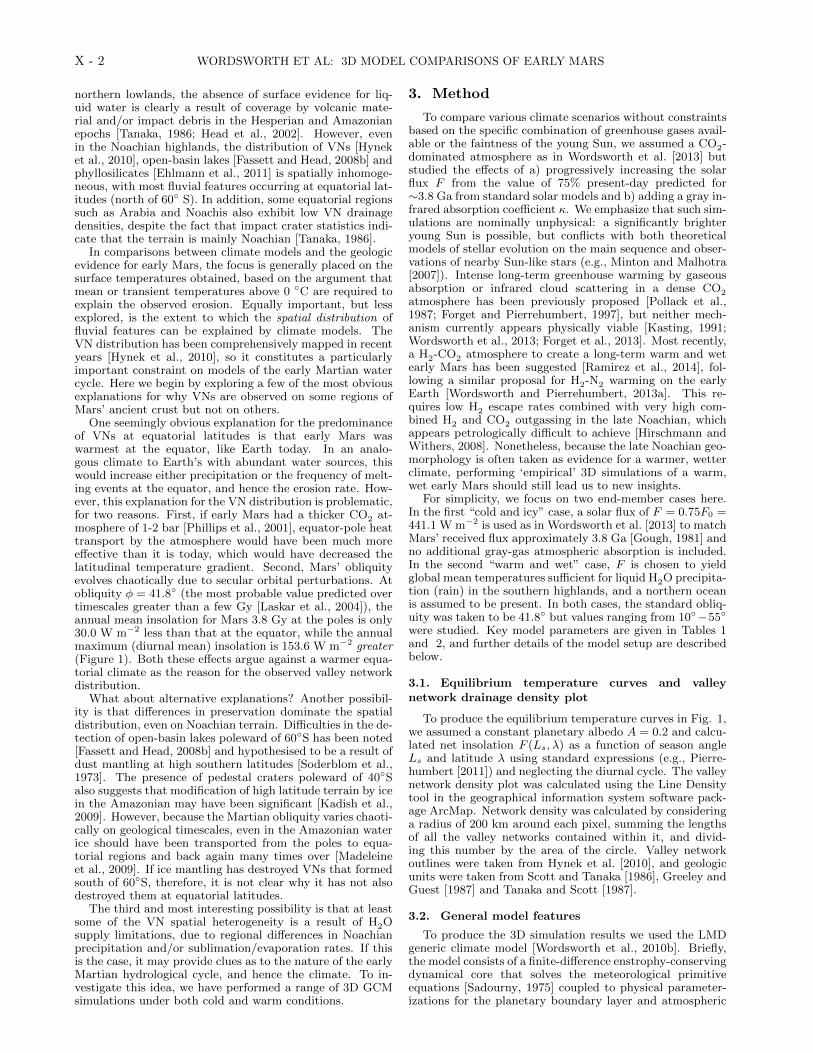
One seemingly obvious explanation for the predominanceof VNs at equatorial latitudes is that early Mars waswarmest at the equator, like Earth today. In an analo-gous climate to Earth’s with abundant water sources, thiswould increase either precipitation or the frequency of melt-ing events at the equator, and hence the erosion rate. How-ever, this explanation for the VN distribution is problematic,for two reasons. First, if early Mars had a thicker CO2 at-mosphere of 1-2 bar [Phillips et al., 2001], equator-pole heattransport by the atmosphere would have been much moreeffective than it is today, which would have decreased thelatitudinal temperature gradient. Second, Mars’ obliquityevolves chaotically due to secular orbital perturbations. Atobliquity φ = 41.8◦ (the most probable value predicted overtimescales greater than a few Gy [Laskar et al., 2004]), theannual mean insolation for Mars 3.8 Gy at the poles is only30.0 W m−2 less than that at the equator, while the annualmaximum (diurnal mean) insolation is 153.6 W m−2 greater(Figure 1). Both these effects argue against a warmer equa-torial climate as the reason for the observed valley networkdistribution.

What about alternative explanations? Another possibil-ity is that differences in preservation dominate the spatialdistribution, even on Noachian terrain. Difficulties in the de-tection of open-basin lakes poleward of 60◦S has been noted[Fassett and Head, 2008b] and hypothesised to be a result ofdust mantling at high southern latitudes [Soderblom et al.,1973]. The presence of pedestal craters poleward of 40◦Salso suggests that modification of high latitude terrain by icein the Amazonian may have been significant [Kadish et al.,2009]. However, because the Martian obliquity varies chaoti-cally on geological timescales, even in the Amazonian waterice should have been transported from the poles to equa-torial regions and back again many times over [Madeleineet al., 2009]. If ice mantling has destroyed VNs that formedsouth of 60◦S, therefore, it is not clear why it has not alsodestroyed them at equatorial latitudes.

The third and most interesting possibility is that at leastsome of the VN spatial heterogeneity is a result of H2Osupply limitations, due to regional differences in Noachianprecipitation and/or sublimation/evaporation rates. If thisis the case, it may provide clues as to the nature of the earlyMartian hydrological cycle, and hence the climate. To in-vestigate this idea, we have performed a range of 3D GCMsimulations under both cold and warm conditions.

3. Method

To compare various climate scenarios without constraintsbased on the specific combination of greenhouse gases avail-able or the faintness of the young Sun, we assumed a CO2-dominated atmosphere as in Wordsworth et al. [2013] butstudied the effects of a) progressively increasing the solarflux F from the value of 75% present-day predicted for∼3.8 Ga from standard solar models and b) adding a gray in-frared absorption coefficient κ. We emphasize that such sim-ulations are nominally unphysical: a significantly brighteryoung Sun is possible, but conflicts with both theoreticalmodels of stellar evolution on the main sequence and obser-vations of nearby Sun-like stars (e.g., Minton and Malhotra[2007]). Intense long-term greenhouse warming by gaseousabsorption or infrared cloud scattering in a dense CO2

atmosphere has been previously proposed [Pollack et al.,1987; Forget and Pierrehumbert, 1997], but neither mech-anism currently appears physically viable [Kasting, 1991;Wordsworth et al., 2013; Forget et al., 2013]. Most recently,a H2-CO2 atmosphere to create a long-term warm and wetearly Mars has been suggested [Ramirez et al., 2014], fol-lowing a similar proposal for H2-N2 warming on the earlyEarth [Wordsworth and Pierrehumbert, 2013a]. This re-quires low H2 escape rates combined with very high com-bined H2 and CO2 outgassing in the late Noachian, whichappears petrologically difficult to achieve [Hirschmann andWithers, 2008]. Nonetheless, because the late Noachian geo-morphology is often taken as evidence for a warmer, wetterclimate, performing ‘empirical’ 3D simulations of a warm,wet early Mars should still lead us to new insights.

For simplicity, we focus on two end-member cases here.In the first “cold and icy” case, a solar flux of F = 0.75F0 =441.1 W m−2 is used as in Wordsworth et al. [2013] to matchMars’ received flux approximately 3.8 Ga [Gough, 1981] andno additional gray-gas atmospheric absorption is included.In the second “warm and wet” case, F is chosen to yieldglobal mean temperatures sufficient for liquid H2O precipita-tion (rain) in the southern highlands, and a northern oceanis assumed to be present. In both cases, the standard obliq-uity was taken to be 41.8◦ but values ranging from 10◦−55◦

were studied. Key model parameters are given in Tables 1and 2, and further details of the model setup are describedbelow.

3.1. Equilibrium temperature curves and valleynetwork drainage density plot

To produce the equilibrium temperature curves in Fig. 1,we assumed a constant planetary albedo A = 0.2 and calcu-lated net insolation F (Ls, λ) as a function of season angleLs and latitude λ using standard expressions (e.g., Pierre-humbert [2011]) and neglecting the diurnal cycle. The valleynetwork density plot was calculated using the Line Densitytool in the geographical information system software pack-age ArcMap. Network density was calculated by consideringa radius of 200 km around each pixel, summing the lengthsof all the valley networks contained within it, and divid-ing this number by the area of the circle. Valley networkoutlines were taken from Hynek et al. [2010], and geologicunits were taken from Scott and Tanaka [1986], Greeley andGuest [1987] and Tanaka and Scott [1987].

3.2. General model features

To produce the 3D simulation results we used the LMDgeneric climate model [Wordsworth et al., 2010b]. Briefly,the model consists of a finite-difference enstrophy-conservingdynamical core that solves the meteorological primitiveequations [Sadourny, 1975] coupled to physical parameter-izations for the planetary boundary layer and atmospheric

WORDSWORTH ET AL: 3D MODEL COMPARISONS OF EARLY MARS X - 3

radiative transfer. The latter is solved using a two-streamapproach [Toon et al., 1989] with optical data derived fromline-by-line calculations [Rothman et al., 2009] and inter-polated collision-induced absorption data [Clough et al.,1989; Gruszka and Borysow, 1998; Baranov et al., 2004;Wordsworth et al., 2010a]. We use the same spectral res-olution as in Wordsworth et al. [2013] (32 infrared bandsand 36 visible bands) but an increased spatial resolution of64× 48× 18 (longitude × latitude × altitude).

As before, the model contains three tracer species: CO2ice, H2O ice/liquid and H2O vapour. Local mean CO2 andH2O cloud particle sizes were determined from the amountof condensed material and the number density of cloud con-densation nuclei [CCN ], which was set at 105 kg−1 for CO2ice, 5 × 105 kg−1 for H2O ice and 107 kg−1 for liquid H2Odroplets. The value of [CCN ] is extremely difficult to con-strain for paleoclimate applications. The values we havechosen for H2O are simply best estimates based on compar-ison with observed values on Earth [Hudson and Yum, 2002].The dependence of climate on the assumed value of [CCN ]for both CO2 and H2O are studied in detail in Wordsworthet al. [2013] and Forget et al. [2013].

Convective processes and cloud microphysics were mod-eled in the same way as previously, with the excep-tion of H2O precipitation. This was modeled using theparametrization of Boucher et al. [1995], with the termi-nal velocity of raindrops calculated assuming a dynamic at-mospheric viscosity and gravity appropriate for CO2 andMars, respectively. The Boucher et. al. scheme is morephysically justified than the threshold approach we usedin Wordsworth et al. [2013]; nonetheless in sensitivity tests(Figure 4b) we found that the two schemes produced com-parable time-averaged results.

3.3. Warm and wet simulations

In the warm and wet simulations, a 1 bar average sur-face pressure was assumed. Estimates of the maximumatmospheric CO2 pressure during the Noachian are of or-der 1-2 bar [Phillips et al., 2001; Kite et al., 2014], withone study [Grott et al., 2011] pointing to lower values(∼ 0.25 bar) based on outgassing models that incorporatethe lower estimated oxygen fugacity of typical Martian mag-mas [Hirschmann and Withers, 2008].

The topography was adjusted so that the minimum al-titude was -2.54 km, corresponding to the putative north-ern ocean shoreline based on delta deposit locations from diAchille and Hynek [2010]. All regions at this altitude werethen defined as ‘ocean’: surface albedo was set to 0.07 andan infinite water source was assumed (Figure 2). In addition,the thermal inertia was adjusted to 14500 tiu, correspond-ing to an ocean mixed layer depth of approximately 50 m[Pierrehumbert, 2011]. Horizontal ocean heat transport wasneglected. Including it would have required a dynamic oceansimulator, which was outside the scope of this study. How-ever, at 1 bar atmospheric pressure the meridional atmo-spheric heat transport is already effective, suggesting thatinclusion of ocean heat transport would not significantly al-ter the main conclusions.

On land, runoff of liquid water was assumed to occuronce the column density in a gridpoint exceeded qmax,surf =150 kg m−2, while the soil dryness threshold was taken tobe 75 kg m−2, corresponding to subsurface liquid water lay-ers of 15 cm and 7.5 cm, respectively. These values werechosen based on Earth GCM modeling [Manabe, 1969], andare reasonable first estimates given our simplified hydrol-ogy scheme and lack of knowledge of late Noachian subsur-face conditions. The sensitivity of the results to the runoffthreshold are investigated in Section 4.4.

The ice-albedo feedback was neglected in the warm andwet simulations by setting the albedo of snow/ice to thesame value as that of rock (0.2). Its inclusion would have

increased the chance of significant glaciation occurring inthe simulations for a given solar flux or atmospheric infraredopacity and hence made a warm, wet Mars even more diffi-cult to achieve. An investigation of the stability of an opennorthern ocean on early Mars to runaway glaciation will begiven in future work.

Finally, for the idealised equatorial mountain simulationsthat were run to study the effect of Tharsis on the hydro-logical cycle, we used

φ(θ, λ) = 2× 103ge−(χ/40◦)2 (1)

with χ2 = (θ + 100◦)2 + λ2, and longitude θ and latitudeλ expressed in degrees. This describes a flat surface with aGaussian height perturbation of full width at half maximum66.6◦ centered at 0◦ N and 100◦ W.

3.4. Cold and icy simulations

In the cold and icy simulations, 0.6 bar average surfacepressure was assumed. This value was chosen as the mini-mum necessary to ensure atmospheric stability against col-lapse of CO2 on the surface for a wide range of obliquities.In some simulations, CO2 ice appeared in specific regions onthe surface all year round. However, secular increases in thetotal surface CO2 ice volume after multiple years were notobserved.

The local stability of surface ice on a cold planet is con-trolled by two parameters: the accumulation rate and thesublimation rate. The sublimation rate can be calculatedbased only on the near-surface temperature, humidity, andwind speed. Calculating the accumulation rate, in contrast,requires a fully integrated (and computationally expensive)representation of the hydrological system. In Wordsworthet al. [2013], we handled this problem using an ice evolutionalgorithm. We ran the climate model with a full water cyclefor several years, calculating the tendencies for sublimationand accumulation. We then multiplied them by a factor be-tween 10 and 100 and restarted the process until the systemapproached an equilibrium state.

Here, the increased spatial resolution of our model makeseven this method prohibitively expensive computationally.Instead, we calculated ice accumulation rates with a fullwater cycle in two scenarios with different ice initial condi-tions [ a) polar source regions and b) an H2O source below-2.54 km (the ‘frozen ocean’ scenario)]. We also computedannual average potential sublimation rates for a wide rangeof parameters in simulations without a water cycle.

We discovered that surface thermodynamics are far moreimportant than the details of the large-scale circulation forgoverning the surface ice evolution in the model, leading toa situation where the spatial distribution of potential sub-limation rates is inversely correlated with that of snow ac-cumulation rates. This means that we can identify placeswhere ice will stabilize in the long term far more rapidlythan is possible using an ice evolution algorithm. Maps ofpotential sublimation can thus be used as a diagnostic forinvestigating the spatial distribution of stable ice.

Quantitatively, we define the potential sublimation as themaximum possible H2O mass flux from the surface to theatmosphere

Spot ≡ −CD|v|RH2O

Tapsat(Ts), (2)

assuming a) that the surface is an infinite source and b)that the atmospheric relative humidity is zero. Here RH2O

is the specific gas constant for H2O. The quantities |v|,Ta and Ts (the surface wind speed, the temperature of thelowest atmospheric layer and the surface temperature, re-spectively) were derived directly from the 3D model outputand psat (the saturation vapour pressure) was derived from


the Clausius-Clayperon relation. The drag coefficient CD is

defined (in neutrally stable conditions) as CD =(

Kln[z/z0]

)2

,

where K = 0.4 is the von Karman constant, z0 is the rough-ness height, and z is the height of the first atmospheric layer.CD was set to a constant 2.75 × 10−3 based on compari-son with the GCM value, which itself was calculated usinga fixed roughness length of 10−2 m. Finally, we integrateSpot over one Martian year to give the theoretical maximumquantity of surface snow/ice that can be sublimated as afunction of longitude and latitude. Our approach to calcu-lating Spot is accurate as long as the atmospheric thermody-namics is not strongly affected by the presence of H2O. Thisis the case for a cold early Mars, which has a surface moistconvection numberM of much less than unity [Wordsworthand Pierrehumbert, 2013b].

To produce estimates of transient melting in the cold, icyscenario, we performed simulations where we started fromthe baseline cold climate state and allowed the system toevolve after altering various parameters. The melting eventsimulations that included dust (Section 4.6) used the samemethod as in Forget et al. [2013], with the total atmosphericoptical depth at the reference wavelength (0.7 µm) set to 5.The value of e = 0.125 in the high eccentricity simulationswas chosen with reference to the orbital evolution calcu-lations of Laskar et al. [2004]. The increase of solar fluxfrom the baseline value of 0.75F0 to 0.8F0 in some of thesimulations is justified given the uncertainty in the abso-lute timing of valley network formation as estimated fromcrater statistics [Fassett and Head, 2008a]. For some sim-ulations, the surface albedo was reduced. The rock albedoAr was taken to be that of basalt (0.1; plausibly the Mar-tian surface was richer in mafic minerals in the Noachian era[Mischna et al., 2013]), while the ice albedo Ai was taken tobe 0.3 (an approximate lower limit for ice contaminated bydust and volcanic ash deposition; Conway et al. [1996]). Thesimulations including SO2 radiative forcing used the samecorrelated-k method as used for the CO2-H2O atmospheres,except that 10 ppmv of SO2 was assumed to be present atall temperature, pressure and H2O mixing ratio values cal-culated. SO2 absorption spectra were obtained from the HI-TRAN database [Rothman et al., 2009], and the differencesin line broadening due to the presence of CO2 as the dom-inant background gas were neglected. Finally, the surfacealbedo was increased to Ai and a thermal inertia appro-priate to solid ice (2000 tiu) was assumed in regions wheremore than 33 kg m−2 (3.3 cm) of surface H2O was present[Le Treut and Li, 1991]. This implies a quite rapid increaseof surface thermal inertia with snow deposition, which makesour results on the rate of summertime snowmelt in the coldscenario (Section 4.6) conservative. We also neglected fur-ther surface radiative effects such as insulation by a surfacesnow layer or solid-state greenhouse warming by ice, bothof which could potentially cause some additional melting.

4. Results

4.1. Overview

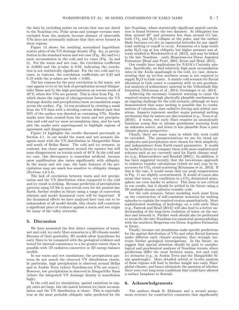
In our cold simulations, surface temperature is con-strained by a fully self-consistent climate model, whereas inthe warm, wet simulations, we can choose surface tempera-ture by varying the solar flux and/or added gray opacity ofthe atmosphere. Fig. 3 shows annual mean surface temper-atures in the two standard scenarios, given obliquity 41.8◦.In the cold case, surface pressure is 0.6 bar and solar fluxis 0.75 times the present day value, while in the warm casethe pressure is 1 bar and the solar flux is 1.3 times presentday. Warm simulations where we used the best-estimateNoachian solar flux but added gray longwave opacity to theatmosphere showed broadly similar results (see Figure 9c).

As can be seen, in both cases adiabatic cooling influencessurface temperature. In the cold, icy scenario, the tem-peratures in the southern hemisphere are partly affected by

seasonal condensation of CO2. In the warm, wet scenario,horizontal temperature variations in the northern and Hel-las basin oceans are low despite the absence of dynamicalocean heat transport, because heat transport by the 1 baratmosphere is efficient. Global mean surface temperatureis 225.5 K for the cold scenario and 282.9 K for the warmscenario.

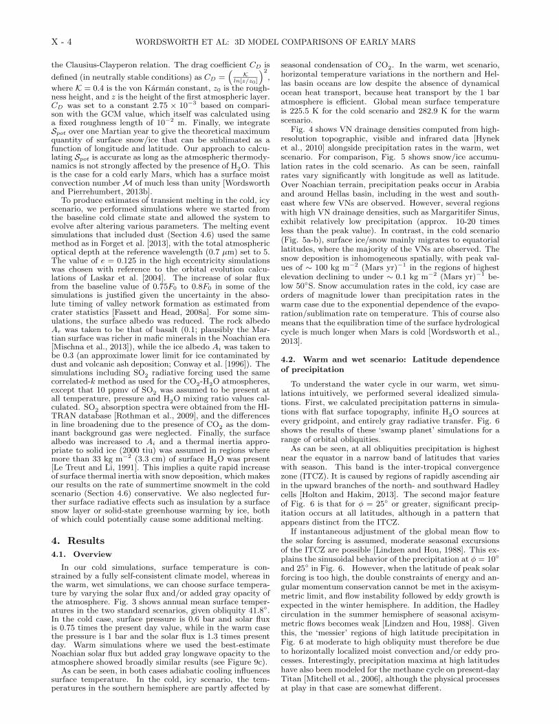
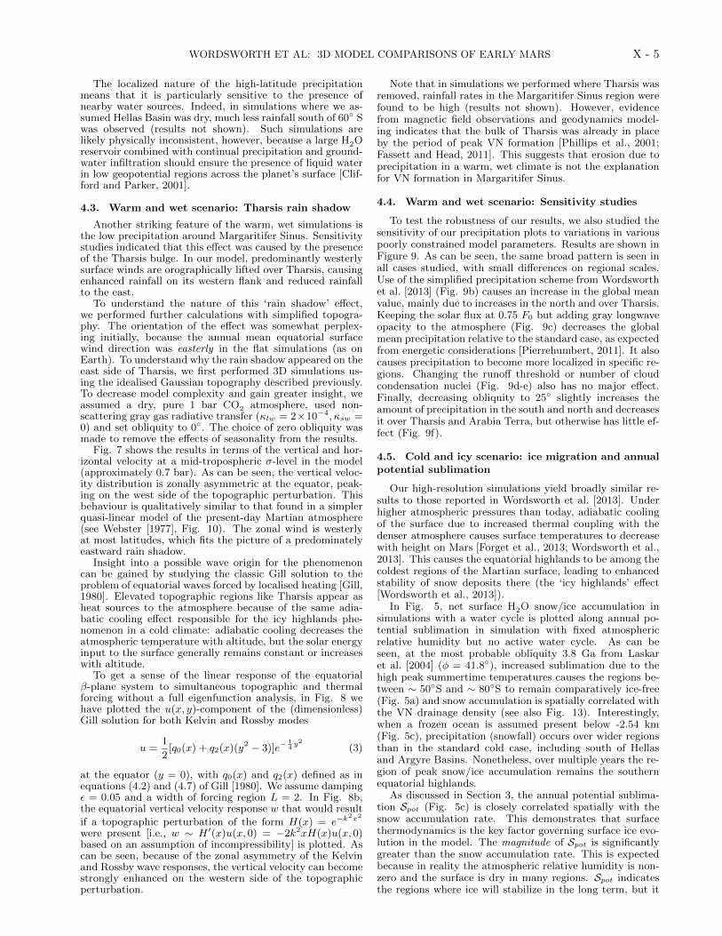
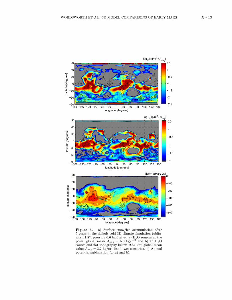
Fig. 4 shows VN drainage densities computed from high-resolution topographic, visible and infrared data [Hyneket al., 2010] alongside precipitation rates in the warm, wetscenario. For comparison, Fig. 5 shows snow/ice accumu-lation rates in the cold scenario. As can be seen, rainfallrates vary significantly with longitude as well as latitude.Over Noachian terrain, precipitation peaks occur in Arabiaand around Hellas basin, including in the west and south-east where few VNs are observed. However, several regionswith high VN drainage densities, such as Margaritifer Sinus,exhibit relatively low precipitation (approx. 10-20 timesless than the peak value). In contrast, in the cold scenario(Fig. 5a-b), surface ice/snow mainly migrates to equatoriallatitudes, where the majority of the VNs are observed. Thesnow deposition is inhomogeneous spatially, with peak val-ues of ∼ 100 kg m−2 (Mars yr)−1 in the regions of highestelevation declining to under ∼ 0.1 kg m−2 (Mars yr)−1 be-low 50◦S. Snow accumulation rates in the cold, icy case areorders of magnitude lower than precipitation rates in thewarm case due to the exponential dependence of the evapo-ration/sublimation rate on temperature. This of course alsomeans that the equilibration time of the surface hydrologicalcycle is much longer when Mars is cold [Wordsworth et al.,2013].

4.2. Warm and wet scenario: Latitude dependenceof precipitation

To understand the water cycle in our warm, wet simu-lations intuitively, we performed several idealized simula-tions. First, we calculated precipitation patterns in simula-tions with flat surface topography, infinite H2O sources atevery gridpoint, and entirely gray radiative transfer. Fig. 6shows the results of these ‘swamp planet’ simulations for arange of orbital obliquities.

As can be seen, at all obliquities precipitation is highestnear the equator in a narrow band of latitudes that varieswith season. This band is the inter-tropical convergencezone (ITCZ). It is caused by regions of rapidly ascending airin the upward branches of the north- and southward Hadleycells [Holton and Hakim, 2013]. The second major featureof Fig. 6 is that for φ = 25◦ or greater, significant precip-itation occurs at all latitudes, although in a pattern thatappears distinct from the ITCZ.

If instantaneous adjustment of the global mean flow tothe solar forcing is assumed, moderate seasonal excursionsof the ITCZ are possible [Lindzen and Hou, 1988]. This ex-plains the sinusoidal behavior of the precipitation at φ = 10◦

and 25◦ in Fig. 6. However, when the latitude of peak solarforcing is too high, the double constraints of energy and an-gular momentum conservation cannot be met in the axisym-metric limit, and flow instability followed by eddy growth isexpected in the winter hemisphere. In addition, the Hadleycirculation in the summer hemisphere of seasonal axisym-metric flows becomes weak [Lindzen and Hou, 1988]. Giventhis, the ‘messier’ regions of high latitude precipitation inFig. 6 at moderate to high obliquity must therefore be dueto horizontally localized moist convection and/or eddy pro-cesses. Interestingly, precipitation maxima at high latitudeshave also been modeled for the methane cycle on present-dayTitan [Mitchell et al., 2006], although the physical processesat play in that case are somewhat different.


The localized nature of the high-latitude precipitationmeans that it is particularly sensitive to the presence ofnearby water sources. Indeed, in simulations where we as-sumed Hellas Basin was dry, much less rainfall south of 60◦ Swas observed (results not shown). Such simulations arelikely physically inconsistent, however, because a large H2Oreservoir combined with continual precipitation and ground-water infiltration should ensure the presence of liquid waterin low geopotential regions across the planet’s surface [Clif-ford and Parker, 2001].

4.3. Warm and wet scenario: Tharsis rain shadow

Another striking feature of the warm, wet simulations isthe low precipitation around Margaritifer Sinus. Sensitivitystudies indicated that this effect was caused by the presenceof the Tharsis bulge. In our model, predominantly westerlysurface winds are orographically lifted over Tharsis, causingenhanced rainfall on its western flank and reduced rainfallto the east.

To understand the nature of this ‘rain shadow’ effect,we performed further calculations with simplified topogra-phy. The orientation of the effect was somewhat perplex-ing initially, because the annual mean equatorial surfacewind direction was easterly in the flat simulations (as onEarth). To understand why the rain shadow appeared on theeast side of Tharsis, we first performed 3D simulations us-ing the idealised Gaussian topography described previously.To decrease model complexity and gain greater insight, weassumed a dry, pure 1 bar CO2 atmosphere, used non-scattering gray gas radiative transfer (κlw = 2×10−4, κsw =0) and set obliquity to 0◦. The choice of zero obliquity wasmade to remove the effects of seasonality from the results.

Fig. 7 shows the results in terms of the vertical and hor-izontal velocity at a mid-tropospheric σ-level in the model(approximately 0.7 bar). As can be seen, the vertical veloc-ity distribution is zonally asymmetric at the equator, peak-ing on the west side of the topographic perturbation. Thisbehaviour is qualitatively similar to that found in a simplerquasi-linear model of the present-day Martian atmosphere(see Webster [1977], Fig. 10). The zonal wind is westerlyat most latitudes, which fits the picture of a predominatelyeastward rain shadow.

Insight into a possible wave origin for the phenomenoncan be gained by studying the classic Gill solution to theproblem of equatorial waves forced by localised heating [Gill,1980]. Elevated topographic regions like Tharsis appear asheat sources to the atmosphere because of the same adia-batic cooling effect responsible for the icy highlands phe-nomenon in a cold climate: adiabatic cooling decreases theatmospheric temperature with altitude, but the solar energyinput to the surface generally remains constant or increaseswith altitude.

To get a sense of the linear response of the equatorialβ-plane system to simultaneous topographic and thermalforcing without a full eigenfunction analysis, in Fig. 8 wehave plotted the u(x, y)-component of the (dimensionless)Gill solution for both Kelvin and Rossby modes

u =1

2[q0(x) + q2(x)(y2 − 3)]e−

14y2 (3)

at the equator (y = 0), with q0(x) and q2(x) defined as inequations (4.2) and (4.7) of Gill [1980]. We assume dampingε = 0.05 and a width of forcing region L = 2. In Fig. 8b,the equatorial vertical velocity response w that would result

if a topographic perturbation of the form H(x) = e−k2x2

were present [i.e., w ∼ H ′(x)u(x, 0) = −2k2xH(x)u(x, 0)based on an assumption of incompressibility] is plotted. Ascan be seen, because of the zonal asymmetry of the Kelvinand Rossby wave responses, the vertical velocity can becomestrongly enhanced on the western side of the topographicperturbation.

Note that in simulations we performed where Tharsis wasremoved, rainfall rates in the Margaritifer Sinus region werefound to be high (results not shown). However, evidencefrom magnetic field observations and geodynamics model-ing indicates that the bulk of Tharsis was already in placeby the period of peak VN formation [Phillips et al., 2001;Fassett and Head, 2011]. This suggests that erosion due toprecipitation in a warm, wet climate is not the explanationfor VN formation in Margaritifer Sinus.

4.4. Warm and wet scenario: Sensitivity studies

To test the robustness of our results, we also studied thesensitivity of our precipitation plots to variations in variouspoorly constrained model parameters. Results are shown inFigure 9. As can be seen, the same broad pattern is seen inall cases studied, with small differences on regional scales.Use of the simplified precipitation scheme from Wordsworthet al. [2013] (Fig. 9b) causes an increase in the global meanvalue, mainly due to increases in the north and over Tharsis.Keeping the solar flux at 0.75 F0 but adding gray longwaveopacity to the atmosphere (Fig. 9c) decreases the globalmean precipitation relative to the standard case, as expectedfrom energetic considerations [Pierrehumbert, 2011]. It alsocauses precipitation to become more localized in specific re-gions. Changing the runoff threshold or number of cloudcondensation nuclei (Fig. 9d-e) also has no major effect.Finally, decreasing obliquity to 25◦ slightly increases theamount of precipitation in the south and north and decreasesit over Tharsis and Arabia Terra, but otherwise has little ef-fect (Fig. 9f).

4.5. Cold and icy scenario: ice migration and annualpotential sublimation

Our high-resolution simulations yield broadly similar re-sults to those reported in Wordsworth et al. [2013]. Underhigher atmospheric pressures than today, adiabatic coolingof the surface due to increased thermal coupling with thedenser atmosphere causes surface temperatures to decreasewith height on Mars [Forget et al., 2013; Wordsworth et al.,2013]. This causes the equatorial highlands to be among thecoldest regions of the Martian surface, leading to enhancedstability of snow deposits there (the ‘icy highlands’ effect[Wordsworth et al., 2013]).

In Fig. 5, net surface H2O snow/ice accumulation insimulations with a water cycle is plotted along annual po-tential sublimation in simulation with fixed atmosphericrelative humidity but no active water cycle. As can beseen, at the most probable obliquity 3.8 Ga from Laskaret al. [2004] (φ = 41.8◦), increased sublimation due to thehigh peak summertime temperatures causes the regions be-tween ∼ 50◦S and ∼ 80◦S to remain comparatively ice-free(Fig. 5a) and snow accumulation is spatially correlated withthe VN drainage density (see also Fig. 13). Interestingly,when a frozen ocean is assumed present below -2.54 km(Fig. 5c), precipitation (snowfall) occurs over wider regionsthan in the standard cold case, including south of Hellasand Argyre Basins. Nonetheless, over multiple years the re-gion of peak snow/ice accumulation remains the southernequatorial highlands.

As discussed in Section 3, the annual potential sublima-tion Spot (Fig. 5c) is closely correlated spatially with thesnow accumulation rate. This demonstrates that surfacethermodynamics is the key factor governing surface ice evo-lution in the model. The magnitude of Spot is significantlygreater than the snow accumulation rate. This is expectedbecause in reality the atmospheric relative humidity is non-zero and the surface is dry in many regions. Spot indicatesthe regions where ice will stabilize in the long term, but it


gives only an approximate upper limit to the total rates ofice/snow transport. The close correlation of Spot with thesnow accumulation rate in Figs. 5a-b nonetheless validatesits use as a diagnostic for investigating the spatial distribu-tion of stable ice in other situations.

In Figure 10, we show the variation of Spot with obliq-uity and surface pressure (Figure 10). In general, the effectof obliquity on surface ice stability lessens as the pressureincreases, because the atmosphere becomes more effectiveat transporting heat across the surface (Figure 10f). At0.6 bar, the effect of obliquity is still fairly important, withlower values causing lower ice stability at the equator in gen-eral. At φ = 25◦ (Figure 10b) Spot is lower (and hence theice is more stable) in the equatorial highland regions thanon most of the rest of the surface, although the main coldtraps have become the south pole and peak of the Tharsisbulge. At φ = 10◦ (Figure 10a), both the north and southpoles are cold traps and water ice is driven away from equa-torial regions. Indeed, our simulations showed that at thisobliquity CO2 itself is unstable to collapse at the poles, evenfor a surface pressure as high as 0.6 bar.

Transient melting of equatorial H2O under a moderatelydense or thin CO2 atmosphere at low obliquity is there-fore only possible if ice migrates more slowly than obliquityvaries. Variations in the Martian obliquity and eccentric-ity occur on 100,000 yr timescales [Laskar et al., 2004]. Icemigration rates are difficult to constrain because of the non-linear dependence of sublimation rate on surface tempera-ture, but the mean values in our model for 0.6 bar CO2 areof order 1 kg m−2 (Mars yr)−1 or ∼ 1 mm (Mars yr)−1,leading to ∼10,000 Mars yr for the transport of 10 m globalaveraged equivalent of H2O. Unless the Noachian surfacewater inventory was orders of magnitude higher than the∼ 34 m estimated to be present today, which may be un-likely [Carr and Head, 2014], the equator would thereforehave been mainly dry at low obliquity. Hence in the cold,icy scenario for early Mars, equatorial melting events shouldonly occur when the obliquity is 25◦ or greater and/or at-mospheric pressure is high.

4.6. Cold and icy scenario: episodic melting events

If early Mars was indeed mainly cold, some mechanismsmust still have been responsible for episodic melting. Possi-ble candidates include seasonal and diurnal effects [Richard-son and Mischna, 2005; Wordsworth et al., 2013], positive ra-diative forcing from atmospheric dust and/or clouds [Forgetand Pierrehumbert, 1997; Pierrehumbert and Erlick, 1998;Urata and Toon, 2013], orbital variations, meteorite impacts[Segura et al., 2008; Toon et al., 2010] and SO2/H2S emis-sion from volcanism [Postawko and Kuhn, 1986; Mischnaet al., 2013; Halevy and Head, 2014; Kerber et al., 2015].

Episodic impact events were an indisputable feature ofthe late Noachian environment, and they may also have hada significant effect on climate. Testing of the hypothesis thatimpacts caused melting sufficient to carve the valley net-works requires 3D modeling of climate across extreme tem-perature ranges, which we plan to address in future work.However, it is worth noting that the stable impact-inducedrunaway greenhouse atmospheres for early Mars proposedrecently [Segura et al., 2012] are highly unlikely. The con-clusion of runaway bistability for early Mars is based onthe assumption of radiative equilibrium in the low atmo-sphere, which requires unphysically high supersaturation ofwater vapour [Nakajima et al., 1992]. Under more realis-tic assumptions for atmospheric relative humidity, the smalldecrease in outgoing longwave radiation with surface tem-perature past the peak value in a clear sky runaway green-house atmosphere is not sufficient for hysteresis under earlyMartian conditions [Pierrehumbert, 2011].

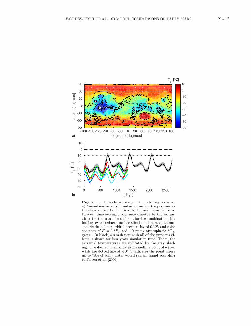
We have systematically studied all the other effects men-tioned above (Fig. 11; see also Wordsworth et al. [2013];Forget et al. [2013]; Kerber et al. [2015]). Alone, they are notsufficient to cause global warming sufficient to explain theobservations. This is clear from Fig. 11b, which shows thediurnal mean temperature vs. time averaged over the region0◦W–120◦ W, 10◦N–30◦ S (see box in Fig. 11a). The cyanline indicates the standard model, while the other coloursindicate runs where effects were added separately [reducedsurface albedo and increased atmospheric dust, blue; orbitaleccentricity of 0.125 and solar constant of F = 0.8F0, red;10 ppmv atmospheric SO2, green]. We find significantlylower warming by SO2 than was reported in Halevy andHead [2014], primarily because our 3D model accounts forthe horizontal transport of heat by the atmosphere awayfrom equatorial regions (see also Kerber et al. [2015]).

The maximum diurnal mean temperature for any of thestudied cases is −20◦ C (for the increased eccentricity andF = 0.8F0 run), implying very limited melting due to anysingle climate forcing mechanism. In combination, however,these effects can cause summertime mean temperatures torise close to 0◦C in the valley network regions. This is shownby the black line in Fig. 11b; the gray envelope indicatesthe maximum and minimum diurnal temperatures.

Figure 12 shows the average quantity of surface liquid wa-ter in the maximum forcing case as a function of time, as-suming a melting point of 0◦C (black line) and -10◦C (blueline). Uncertainty in the freezing point of early Martian icedue to the presence of solutes means that a melting thresholdof -10◦C is reasonable in a mainly cold scenario [Fairen et al.,2009]. As can be seen peak melting reaches 5-7 kg m−2 insummertime in the briny case. This is still significantly be-low the 150 kg m−2 runoff threshold used in the warm andwet simulations, which itself was based on estimates fromwarm regions on Earth lacking subsurface permafrost.

Hoke et al. [2011] estimate that intermittent runoff ratesof a few cm/day on timescales of order 105 to 107 years arenecessary to explain the largest Noachian VNs. Our meltingestimates are somewhat below these values, even if runoffis assumed to occur almost instantaneously after melting.Nonetheless, the exponential dependence of melting rate ontemperature means that only a slight increase in forcing be-yond that used to produce Fig. 12 would bring the modelpredictions into the necessary regime. Furthermore, the de-tails of melting processes in marginally warm scenarios maystill allow for significant fluvial erosion, as evidenced by ge-omorphic studies of the McMurdo Dry Valleys in Antarctica[Head and Marchant, 2014] and recent modeling of top-downmelting from a late Noachian icesheet [Fastook and Head,2014]. Incorporation of a more sophisticated hydrologicalscheme in the model in future incorporating e.g. hyporheicprocesses will allow these issues to be investigated in moredetail.

In this analysis, we do not claim to have uniquely iden-tified the key warming processes in the late Noachian cli-mate. Nonetheless, we have demonstrated that melting ina cold, icy scenario is possible using combinations of phys-ically plausible mechanisms. In contrast, achieving contin-uous warm and wet conditions is much more difficult, asdemonstrated by our simulations, which require an increasedsolar flux compared to present day (in conflict with basicstellar physics) and/or intense greenhouse warming in addi-tion to that provided by a 1-bar CO2 atmosphere.

4.7. Spatial correlation of valley networks withrainfall and snow accumulation rates

Because the model predictions for precipitation in thewarm, wet regime and snow accumulation in the cold, icyregime are quite different, it is interesting to compare thespatial correlations with the Hynek et al. valley networkdrainage density in each case. To do this, we first filtered


the data by excluding points on terrain that was not datedto the Noachian era. Polar areas and younger terrains wereexcluded from the analysis because absence of observableVNs does not necessarily indicate that they never formed inthese regions.

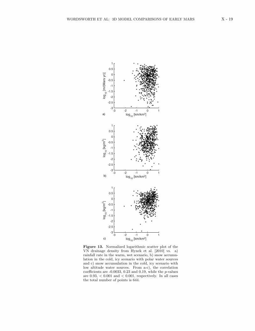
Figure 13 shows the resulting normalized logarithmicscatter plots of the VN drainage density (Fig. 4a), a) precip-itation in the standard warm and wet case (Fig. 4b) and b-c)snow accumulation in the cold and icy cases (Fig. 5a andb). For the warm and wet case, the correlation coefficientis -0.0033 and the p-value is 0.93, indicating the correla-tion is not statistically significant. For the two cold and icycases, in contrast, the correlation coefficients are 0.23 and0.19 while the p-values are both < 0.001.

The key reasons for the poor correlation in the warm, wetcase appear to be a) the lack of precipitation around Margar-itifer Sinus and b) the high precipitation on terrain south of40◦S, where few VNs are present. This is clear from Fig. 14,which shows the regions of (dis)agreement between the VNdrainage density and precipitation/snow accumulation mapsacross the surface. Fig. 14 was produced by creating a maskfrom the VN data with a dividing contour defined such that50% of the surface was denoted as containing VNs. Similarmasks were then created from the warm and wet precipita-tion and cold and icy snow accumulation data, and for eachplot the masks were superimposed to highlight regions ofagreement and disagreement.

Figure 14 highlights the results discussed previously inSection 4.1: in our model the warm and wet scenario dis-agrees most with the VN distribution in Margaritifer Sinusand south of Hellas Basin. The cold and icy scenario, incontrast, has closer agreement around the equator but stillsome disagreement on terrain south of 40◦S. In the cold andicy case, this discrepancy is somewhat artificial, becausesnow equilibration also varies significantly with obliquity.In the warm and wet case, the basic features of the pre-cipitation map are much less sensitive to obliquity changes(Sections 4.2-4.4).

The lack of correlation between warm and wet precipi-tation and the VN distribution when compared to the coldand icy result is striking. Because prediction of precipitationpatterns using GCMs is non-trivial even for the present-dayEarth, further studies in future using a range of convectionschemes and model dynamical cores will be important. Ifthe dynamical effects we have analyzed here turn out to beindependent of all model details, this clearly will constitutea significant piece of evidence against a warm and wet originfor many of the valley networks.

5. Discussion

We have presented the first direct comparison of warm,wet and cold, icy early Mars scenarios in a 3D climate model.Because of their generality, 3D models allow hypotheses forearly Mars to be compared with the geological evidence andtested for internal consistency to a far greater extent than ispossible with 1D radiative-convective or 2D energy-balancemodels.

In our warm and wet simulations, the precipitation pat-terns do not match the observed VN distribution closely.In particular, high precipitation is observed around Hellasand in Arabia Terra (where Noachian-era VNs are scarce).However, low precipitation is observed in Margaritifer Sinus(where the integrated VN drainage density is nonethelesshigh).

In the cold and icy simulations, spatial variations in sup-ply rates are large, but the match between ice/snow accumu-lation and the VN distribution is closer. This is especiallytrue at the most probable obliquity value predicted for the

late Noachian, where statistically significant spatial correla-tion is found between the two datasets. At obliquities lessthan around 20◦ and pressures less than around 0.5 bar,both CO2 and H2O collapse at the poles, and the surfacelikely becomes too dry at equatorial latitudes for any signif-icant melting or runoff to occur. Formation of a large southpolar H2O cap at low obliquity but higher pressure was al-ready studied in Wordsworth et al. [2013], and may be linkedto the late Noachian – early Hesperian-era Dorsa ArgenteaFormation [Head and Pratt, 2001; Kress and Head, 2015].

Our results have implications for NASA’s Curiosity mis-sion. Specifically, we find relatively high snow accumulationrates in the Aeolis quadrangle in the cold, icy case, demon-strating that an ice-free northern ocean is not required tosupply H2O to Gale crater. A mainly cold scenario for fluvialalteration in Gale crater is consistent with in-situ geochem-ical analyses of sedimentary material in the Yellowknife Bayformation [McLennan et al., 2014; Grotzinger et al., 2014].

Achieving the necessary transient warming to cause therequired erosion through physically plausible mechanisms isan ongoing challenge for the cold scenario, although we havedemonstrated that some melting is possible due to combi-nations of volcanism, dust radiative forcing and orbital vari-ations. Impacts represent another major potential meltingmechanism that by nature are also transient (e.g., Toon et al.[2010]). A warm, wet early Mars requires an anomalouslyluminous young Sun or intense greenhouse warming froman unknown source, and hence is less plausible from a pureclimate physics perspective.

Clearly, there are many ways in which this work couldbe extended. The parametrizations we use for cloud mi-crophysics and precipitation were chosen for their simplicityand independence from Earth-tuned parameters. It wouldbe useful in future to compare them with more sophisticatedschemes such as are currently used for Earth climate stud-ies (e.g., Khairoutdinov and Randall [2001]). In addition, ithas been suggested recently that the two-stream approachto radiative transfer calculations (which we use) may be in-accurate for CO2 cloud scattering [Kitzmann et al., 2013]. Ifthis is the case, it would mean that our peak temperaturesin Fig. 11 are slightly overestimated. It would of course alsomean that warm, wet conditions in a CO2-dominated atmo-sphere are even harder to achieve. This issue is not criticalto our results, but it should be settled in the future using a3D multiple-stream radiative transfer code.

For the cold scenario, future modeling work must focuson the construction of self-consistent scenarios for meltingepisodes to explain the required erosion quantitatively. Moresophisticated modeling of hydrology on a cold early Mars(e.g., Fastook and Head [2014]) will also lead to a better un-derstanding of the long-term evolution of water on the sur-face and beneath it. Further work should also be performedto reconcile the late Noachian-era equatorial geomorphologywith the southern Hesperian-era Dorsa Argentea Formationin future.

Finally, because our simulations make specific predictionsfor the spatial distribution of VNs and other fluvial featuresunder different early climate scenarios, they strongly mo-tivate further geological investigations. In the future, wesuggest that special attention should be paid to morpho-logical and geochemical analyses of Noachian terrain wherepredictions differ the most between warm, wet and cold,icy scenarios (e.g., in Arabia Terra and the Margaritifer Si-nus quadrangle). More detailed orbital or in-situ analysisof these regions will lead to further insight into early Mars’global climate, and hence ultimately the question of whetherthere were ever long-term conditions that could have alloweda surface biosphere to flourish.

6. Acknowledgements

The authors thank B. Ehlmann and a second anony-mous reviewer for constructive comments that significantly


improved the quality of the manuscript. We also thankEhouarn Millour for help in setting up the parallelized ver-sion of the generic model that was used for some of thesimulations. The computations in this paper were run onthe Odyssey cluster supported by the FAS Division of Sci-ence, Research Computing Group at Harvard University. Alldata and code used to produce the figures in this article areavailable from the lead author on request (contact [email protected]).

References

Y. I. Baranov, W. J. Lafferty, and G. T. Fraser. Infrared spectrumof the continuum and dimer absorption in the vicinity of theO 2 vibrational fundamental in O 2/CO 2 mixtures. Journalof Molecular Spectroscopy, 228:432–440, December 2004. doi:10.1016/j.jms.2004.04.010.

J.-P. Bibring, Y. Langevin, J. F. Mustard, F. Poulet, R. Arvidson,A. Gendrin, B. Gondet, N. Mangold, P. Pinet, and F. Forget.Global Mineralogical and Aqueous Mars History Derived fromOMEGA/Mars Express Data. Science, 312:400–404, April2006. doi: 10.1126/science.1122659.

O. Boucher, H. Le Treut, and M. B. Baker. Precipitation andradiation modeling in a general circulation model: Introduc-tion of cloud microphysical processes. Journal of GeophysicalResearch: Atmospheres (1984–2012), 100(D8):16395–16414,1995.

M. H. Carr. Water on Mars. New York: Oxford University Press,—c1996, 1996.

M. H. Carr and J. W. Head. Martian unbound water inventories:Changes with time. In Lunar and Planetary Institute ScienceConference Abstracts, volume 45, page 1427, 2014.

S. M. Clifford and T. J. Parker. The evolution of the martianhydrosphere: Implications for the fate of a primordial oceanand the current state of the northern plains. Icarus, 154:40–79,November 2001. doi: 10.1006/icar.2001.6671.

S. A. Clough, F. X. Kneizys, and R. W. Davies. Line shape andthe water vapor continuum. Atmospheric Research, 23(3-4):229 – 241, 1989. ISSN 0169-8095.

H. Conway, A. Gades, and C. F. Raymond. Albedo of dirty snowduring conditions of melt. Water Resources Research, 32(6):1713–1718, 1996.

Robert A Craddock and Alan D Howard. The case for rainfallon a warm, wet early mars. Journal of Geophysical Research,107(E11):5111, 2002.

G. di Achille and B. M. Hynek. Ancient ocean on Mars supportedby global distribution of deltas and valleys. Nature Geoscience,3:459–463, July 2010. doi: 10.1038/ngeo891.

B. L. Ehlmann, J. F. Mustard, S. L. Murchie, J.-P. Bibring,A. Meunier, A. A. Fraeman, and Y. Langevin. Subsurfacewater and clay mineral formation during the early history ofMars. Nature, 479:53–60, November 2011. doi: 10.1038/na-ture10582.

Alberto G Fairen, Alfonso F Davila, Luis Gago-Duport, RicardoAmils, and Christopher P McKay. Stability against freezing ofaqueous solutions on early mars. Nature, 459(7245):401–404,2009.

C. I. Fassett and J. W. Head. The timing of mar-tian valley network activity: Constraints from bufferedcrater counting. Icarus, 195:61–89, May 2008a. doi:10.1016/j.icarus.2007.12.009.

C. I. Fassett and J. W. Head. Valley network-fed, open-basin lakeson Mars: Distribution and implications for Noachian surfaceand subsurface hydrology. Icarus, 198:37–56, November 2008b.doi: 10.1016/j.icarus.2008.06.016.

C. I. Fassett and J. W. Head. Sequence and timing of conditionson early Mars. Icarus, 211:1204–1214, February 2011. doi:10.1016/j.icarus.2010.11.014.

J. L. Fastook and J. W. Head. Glaciation in the late noachianicy highlands: Ice accumulation, distribution, flow rates, basalmelting, and top-down melting rates and patterns. Planetaryand Space Science, 2014.

F. Forget and R. T. Pierrehumbert. Warming Early Mars withCarbon Dioxide Clouds That Scatter Infrared Radiation. Sci-ence, 278:1273–+, November 1997.

F. Forget, R. D. Wordsworth, E. Millour, J.-B. Madeleine, L. Ker-ber, J. Leconte, E. Marcq, and R. M. Haberle. 3d modellingof the early martian climate under a denser CO2 atmosphere:Temperatures and CO2 ice clouds. Icarus, 2013.

A. E. Gill. Some simple solutions for heat-induced tropical circu-lation. Quarterly Journal of the Royal Meteorological Society,106(449):447–462, 1980.

D. O. Gough. Solar interior structure and luminosity variations.Solar Physics, 74:21–34, November 1981.

R. Greeley and J. Guest. Geologic map of the eastern equatorialregion of Mars. Geological Survey (US), 1987.

M. Grott, A. Morschhauser, D. Breuer, and E. Hauber. Vol-canic outgassing of CO2 and H2O on Mars. Earth andPlanetary Science Letters, 308:391–400, August 2011. doi:10.1016/j.epsl.2011.06.014.

J. P. Grotzinger, D. Y. Sumner, L. C. Kah, K. Stack, S. Gupta,L. Edgar, D. Rubin, K. Lewis, J. Schieber, N. Mangold,R. Milliken, P. G. Conrad, D. DesMarais, J. Farmer,K. Siebach, F. Calef, J. Hurowitz, S. M. McLennan, D. Ming,D. Vaniman, J. Crisp, A. Vasavada, K. S. Edgett, M. Malin,D. Blake, R. Gellert, P. Mahaffy, R. C. Wiens, S. Mau-rice, J. A. Grant, S. Wilson, R. C. Anderson, L. Beegle,R. Arvidson, B. Hallet, R. S. Sletten, M. Rice, J. Bell,J. Griffes, B. Ehlmann, R. B. Anderson, T. F. Bristow,W. E. Dietrich, G. Dromart, J. Eigenbrode, A. Fraeman,C. Hardgrove, K. Herkenhoff, L. Jandura, G. Kocurek, S. Lee,L. A. Leshin, R. Leveille, D. Limonadi, J. Maki, S. McCloskey,M. Meyer, M. Minitti, H. Newsom, D. Oehler, A. Okon,M. Palucis, T. Parker, S. Rowland, M. Schmidt, S. Squyres,A. Steele, E. Stolper, R. Summons, A. Treiman, R. Williams,A. Yingst, and MSL Science Team. A habitable fluvio-lacustrine environment at yellowknife bay, gale crater, mars.Science, 343(6169), 2014. doi: 10.1126/science.1242777. URLhttp://www.sciencemag.org/content/343/6169/1242777.abstract.

M. Gruszka and A. Borysow. Computer simulation of thefar infrared collision induced absorption spectra of gaseousCO2. Molecular Physics, 93:1007–1016, 1998. doi:10.1080/002689798168709.

I. Halevy and J. W. Head. Episodic warming of early mars bypunctuated volcanism. Nature Geoscience, 2014.

J. W. Head and S. Pratt. Extensive Hesperian-aged south po-lar ice sheet on Mars: Evidence for massive melting and re-treat, and lateral flow and ponding of meltwater. Journalof Geophysical Research, 106:12275–12300, June 2001. doi:10.1029/2000JE001359.

J. W. Head, M. A. Kreslavsky, and S. Pratt. Northern lowlandsof Mars: Evidence for widespread volcanic flooding and tec-tonic deformation in the Hesperian Period. Journal of Geo-physical Research (Planets), 107:5003, January 2002. doi:10.1029/2000JE001445.

James W Head and David R Marchant. The climate history ofearly mars: insights from the antarctic mcmurdo dry valleyshydrologic system. Antarctic Science, 26(06):774–800, 2014.

M. M. Hirschmann and A. C. Withers. Ventilation of CO2 from areduced mantle and consequences for the early martian green-house. Earth and Planetary Science Letters, 270(1):147–155,2008.

M. R. T. Hoke, B. M. Hynek, and G. E. Tucker. Formationtimescales of large martian valley networks. Earth and Plan-etary Science Letters, 312(1):1–12, 2011.

J. R. Holton and G. J. Hakim. An introduction to dynamic me-teorology. Academic press, 2013.

James G Hudson and Seong Soo Yum. Cloud condensation nucleispectra and polluted and clean clouds over the indian ocean.Journal of Geophysical Research: Atmospheres (1984–2012),107(D19):INX2–21, 2002.

B. M. Hynek, M. Beach, and M. R. T. Hoke. Updated global mapof Martian valley networks and implications for climate and hy-drologic processes. Journal of Geophysical Research (Planets),115:E09008, September 2010. doi: 10.1029/2009JE003548.

S. J. Kadish, N. G. Barlow, and J. W. Head. Latitude dependenceof martian pedestal craters: Evidence for a sublimation-drivenformation mechanism. Journal of Geophysical Research: Plan-ets (1991–2012), 114(E10), 2009.

J. F. Kasting. CO2 condensation and the climate of early Mars.Icarus, 94:1–13, November 1991.

L. Kerber, F. Forget, and R. D. Wordsworth. Sulfur in the earlymartian atmosphere revisited: Experiments with a 3-d globalclimate model. Icarus, 2015.


Marat F Khairoutdinov and David A Randall. A cloud resolvingmodel as a cloud parameterization in the ncar community cli-mate system model: Preliminary results. Geophysical ResearchLetters, 28(18):3617–3620, 2001.

E. S. Kite, J.-P. Williams, A. Lucas, and O. Aharonson. Lowpalaeopressure of the martian atmosphere estimated from thesize distribution of ancient craters. Nature Geoscience, 7(5):335–339, 2014.

D. Kitzmann, A. B. C. Patzer, and H. Rauer. Clouds in the atmo-spheres of extrasolar planets. IV. On the scattering greenhouseeffect of CO2 ice particles: Numerical radiative transfer stud-ies. Astronomy & Astrophysics, 557:A6, September 2013. doi:10.1051/0004-6361/201220025.

Ailish M. Kress and James W. Head. Late noachian and earlyhesperian ridge systems in the south circumpolar dorsa ar-gentea formation, mars: Evidence for two stages of melt-ing of an extensive late noachian ice sheet. Planetary andSpace Science, 109–110(0):1 – 20, 2015. ISSN 0032-0633. doi:http://dx.doi.org/10.1016/j.pss.2014.11.025.

J. Laskar, A. C. M. Correia, M. Gastineau, F. Joutel, B. Levrard,and P. Robutel. Long term evolution and chaotic diffusion ofthe insolation quantities of Mars. Icarus, 170:343–364, August2004. doi: 10.1016/j.icarus.2004.04.005.

Herve Le Treut and Zhao-Xin Li. Sensitivity of an atmosphericgeneral circulation model to prescribed sst changes: feed-back effects associated with the simulation of cloud opti-cal properties. Climate Dynamics, 5:175–187, 1991. ISSN0930-7575. URL http://dx.doi.org/10.1007/BF00251808.10.1007/BF00251808.

R. S. Lindzen and A. V. Hou. Hadley circulations for zonallyaveraged heating centered off the equator. Journal of the At-mospheric Sciences, 45(17):2416–2427, 1988.

J.-B. Madeleine, F. Forget, J. W. Head, B. Levrard,F. Montmessin, and E. Millour. Amazonian north-ern mid-latitude glaciation on Mars: A proposed cli-mate scenario. Icarus, 203:390–405, October 2009. doi:10.1016/j.icarus.2009.04.037.

Syukuro Manabe. Climate and the ocean circulation 1: The at-mospheric circulation and the hydrology of the earth’s surface.Monthly Weather Review, 97(11):739–774, 1969.

N. Mangold, C. Quantin, V. Ansan, C. Delacourt, and P. Alle-mand. Evidence for precipitation on mars from dendritic val-leys in the valles marineris area. Science, 305(5680):78–81,2004.

S. M. McLennan, R. B. Anderson, J. F. Bell, J. C. Bridges,F. Calef, J. L. Campbell, B. C. Clark, S. Clegg, P. Con-rad, A. Cousin, D. J. Des Marais, G. Dromart, M. D.Dyar, L. A. Edgar, B. L. Ehlmann, C. Fabre, O. Forni,O. Gasnault, R. Gellert, S. Gordon, J. A. Grant, J. P.Grotzinger, S. Gupta, K. E. Herkenhoff, J. A. Hurowitz,P. L. King, S. Le Mouelic, L. A. Leshin, R. Leveille, K. W.Lewis, N. Mangold, S. Maurice, D. W. Ming, R. V. Morris,M. Nachon, H. E. Newsom, A. M. Ollila, G. M. Perrett,M. S. Rice, M. E. Schmidt, S. P. Schwenzer, K. Stack,E. M. Stolper, D. Y. Sumner, A. H. Treiman, S. VanBom-mel, D. T. Vaniman, A. Vasavada, R. C. Wiens, R. A.Yingst, and MSL Science Team. Elemental geochemistryof sedimentary rocks at yellowknife bay, gale crater, mars.Science, 343(6169), 2014. doi: 10.1126/science.1244734. URLhttp://www.sciencemag.org/content/343/6169/1244734.abstract.

David A Minton and Renu Malhotra. Assessing the massive youngsun hypothesis to solve the warm young earth puzzle. The As-trophysical Journal, 660(2):1700, 2007.

M. A. Mischna, V. Baker, R. Milliken, M. Richardson, and C. Lee.Effects of obliquity and water vapor/trace gas greenhouses inthe early martian climate. Journal of Geophysical Research:Planets, 2013.

Jonathan L Mitchell, Raymond T Pierrehumbert, Dargan MWFrierson, and Rodrigo Caballero. The dynamics behind titan’smethane clouds. Proceedings of the National Academy of Sci-ences, 103(49):18421–18426, 2006.

J. F. Mustard, S. L. Murchie, S. M. Pelkey, B. L. Ehlmann, R. E.Milliken, J. A. Grant, J.-P. Bibring, F. Poulet, J. Bishop, E. N.Dobrea, L. Roach, F. Seelos, R. E. Arvidson, S. Wiseman,R. Green, C. Hash, D. Humm, E. Malaret, J. A. McGovern,K. Seelos, T. Clancy, R. Clark, D. D. Marais, N. Izenberg,

A. Knudson, Y. Langevin, T. Martin, P. McGuire, R. Mor-ris, M. Robinson, T. Roush, M. Smith, G. Swayze, H. Tay-lor, T. Titus, and M. Wolff. Hydrated silicate minerals onMars observed by the Mars Reconnaissance Orbiter CRISMinstrument. Nature, 454:305–309, July 2008. doi: 10.1038/na-ture07097.

Shinichi Nakajima, Yoshi-Yuki Hayashi, and Yukata Abe. A studyon the erunaway greenhouse effectıwith a one-dimensionalradiative–convective equilibrium model. J. Atmos. Sci, 49:2256–2266, 1992.

R. J. Phillips, M. T. Zuber, S. C. Solomon, M. P. Golombek, B. M.Jakosky, W. B. Banerdt, D. E. Smith, R. M. E. Williams,B. M. Hynek, O. Aharonson, and S. A. Hauck. Ancient geo-dynamics and global-scale hydrology on Mars. Science, 291:2587–2591, March 2001. doi: 10.1126/science.1058701.

R. T. Pierrehumbert. Principles of Planetary Climate. Cam-bridge University Press, 2011. ISBN 9780521865562. URLhttp://books.google.com/books?id=bO U8f5pVR8C.

R. T. Pierrehumbert and C. Erlick. On the scattering greenhouseeffect of co2 ice clouds. Journal of the atmospheric sciences,55(10):1897–1903, 1998.

J. B. Pollack, J. F. Kasting, S. M. Richardson, and K. Poliakoff.The case for a wet, warm climate on early Mars. Icarus, 71:203–224, August 1987. doi: 10.1016/0019-1035(87)90147-3.

S. E. Postawko and W. R. Kuhn. Effect of the greenhouse gases(CO2, H2O, SO2) on martian paleoclimate. Journal of Geo-physical Research, 91:431–D438, September 1986.

R. M. Ramirez, R. Kopparapu, M. E. Zugger, T. D. Robinson,R. Freedman, and J. F. Kasting. Warming early mars withCO2 and H2. Nature Geoscience, 7(1):59–63, 2014.

M. I. Richardson and M. A. Mischna. Long-term evolution oftransient liquid water on mars. Journal of Geophysical Re-search: Planets (1991–2012), 110(E3), 2005.

L. S. Rothman, I. E. Gordon, A. Barbe, D. C. Benner, P. F.Bernath, M. Birk, V. Boudon, L. R. Brown, A. Campargue,J.-P. Champion, K. Chance, L. H. Coudert, V. Dana, V. M.Devi, S. Fally, J.-M. Flaud, R. R. Gamache, A. Goldman,D. Jacquemart, I. Kleiner, N. Lacome, W. J. Lafferty, J.-Y. Mandin, S. T. Massie, S. N. Mikhailenko, C. E. Miller,N. Moazzen-Ahmadi, O. V. Naumenko, A. V. Nikitin, J. Or-phal, V. I. Perevalov, A. Perrin, A. Predoi-Cross, C. P. Rins-land, M. Rotger, M. Simeckova, M. A. H. Smith, K. Sung,S. A. Tashkun, J. Tennyson, R. A. Toth, A. C. Vandaele, andJ. Vander Auwera. The HITRAN 2008 molecular spectroscopicdatabase. Journal of Quantitative Spectroscopy and RadiativeTransfer, 110:533–572, 2009. doi: 10.1016/j.jqsrt.2009.02.013.

R. Sadourny. The Dynamics of Finite-Difference Models of theShallow-Water Equations. Journal of Atmospheric Sciences,32:680–689, 1975.

C. Sagan and G. Mullen. Earth and Mars: Evolution of Atmo-spheres and Surface Temperatures. Science, 177:52–56, 1972.doi: 10.1126/science.177.4043.52.

D. H. Scott and K. L. Tanaka. Geologic map of the western equa-torial region of Mars. Geological Survey (US), 1986.

T. L. Segura, O. B. Toon, and A. Colaprete. Modeling the en-vironmental effects of moderate-sized impacts on Mars. Jour-nal of Geophysical Research (Planets), 113:E11007, November2008. doi: 10.1029/2008JE003147.

Teresa L Segura, Christopher P McKay, and Owen B Toon. Animpact-induced, stable, runaway climate on mars. Icarus, 220(1):144–148, 2012.

L. A. Soderblom, T. J. Kreidler, and H. Masursky. Latitudinaldistribution of a debris mantle on the martian surface. Journalof Geophysical Research, 78(20):4117–4122, 1973.

S. W. Squyres and J. F. Kasting. Early Mars: How Warmand How Wet? Science, 265:744–749, August 1994. doi:10.1126/science.265.5173.744.

K. L. Tanaka. The stratigraphy of mars. Journal of Geophysi-cal Research: Solid Earth (1978–2012), 91(B13):E139–E158,1986.

K. L. Tanaka and D. H. Scott. Geologic map of the polar regionsof Mars. Geological Survey (US), 1987.

O. B. Toon, C. P. McKay, T. P. Ackerman, and K. Santhanam.Rapid calculation of radiative heating rates and photodissoci-ation rates in inhomogeneous multiple scattering atmospheres.Journal of Geophysical Research, 94:16287–16301, November1989.

O. B. Toon, T. Segura, and K. Zahnle. The formation of martianriver valleys by impacts. Annual Review of Earth and Plan-etary Sciences, 38:303–322, May 2010. doi: 10.1146/annurev-earth-040809-152354.


R. A. Urata and O. B. Toon. Simulations of the martian hydro-logic cycle with a general circulation model: Implications forthe ancient martian climate. Icarus, 2013.

P. J. Webster. The low-latitude circulation of mars. Icarus, 30(4):626–649, 1977.

R. M. E. Williams, J. P. Grotzinger, W. E. Dietrich, S. Gupta,D. Y. Sumner, R. C. Wiens, N. Mangold, M. C. Malin, K. S.Edgett, S. Maurice, et al. Martian fluvial conglomerates atgale crater. Science, 340(6136):1068–1072, 2013.

R. Wordsworth and R. Pierrehumbert. Hydrogen-nitrogengreenhouse warming in earth’s early atmosphere. Science,339(6115):64–67, 2013a. doi: 10.1126/science.1225759. URLhttp://www.sciencemag.org/content/339/6115/64.abstract.

R. Wordsworth and R. Pierrehumbert. Water loss from terres-trial planets with CO2-rich atmospheres. The AstrophysicalJournal, 778(2):154, 2013b.

R. Wordsworth, F. Forget, and V. Eymet. Infrared collision-induced and far-line absorption in dense CO2 atmo-spheres. Icarus, 210:992–997, December 2010a. doi:10.1016/j.icarus.2010.06.010.

R. Wordsworth, F. Forget, F. Selsis, J.-B. Madeleine, E. Mil-lour, and V. Eymet. Is Gliese 581d habitable? Some con-straints from radiative-convective climate modeling. Astron-omy and Astrophysics, 522:A22+, 2010b. doi: 10.1051/0004-6361/201015053.

R. Wordsworth, F. Forget, E. Millour, J. W. Head, J.-B.Madeleine, and B. Charnay. Global modelling of the earlymartian climate under a denser CO2 atmosphere: Water cycleand ice evolution. Icarus, 222(1):1–19, 2013.

Table 1. Parameters used in the warm and wet climate simulations. Bold indicates the values for the ‘standard’ simulations.

Surface pressure 1 barSolar flux 441.1, 764.5 W m−2

Added atmospheric gray mass absorption coefficient 0.0, 2.0×10−4 m2 kg−1

Orbital obliquity 25.0◦, 41.8◦

Orbital eccentricity 0.0Runoff threshold 1, 150 kg m−2

Table 2. Parameters used in the cold and icy climate simulations. Bold indicates the values for the ‘standard’ simulations.

Surface pressure 0.125, 0.6, 2 barSolar flux 441.1 W m−2, 470.5 W m−2,

Orbital obliquity 10.0◦, 25.0◦, 41.8◦, 55.0◦

Orbital eccentricity 0.0, 0.125Atmospheric SO2 0.0, 10.0 ppmv

Dust optical depth at 0.7 µm 0.0, 5.0

−90 −60 −30 0 30 60 9050

100

150

200

250

300

350

400

450

500

550

[W/m

2 ]

latitude [degrees]−90 −60 −30 0 30 60 90

200

220

240

260

280

300

T [K

]

latitude [degrees]

Figure 1. (left) Insolation vs. latitude for Earth (black)and early Mars with obliquity 25.0◦ (red) and 41.8◦

(blue). Solid and dashed lines denote annual mean andannual maximum (diurnal mean) temperatures, respec-tively. For Earth the obliquity is 23.4◦. In both cases analbedo of 0.2 and orbital eccentricity of 0.0 is assumed,while for early Mars the solar constant is taken to be 0.75times the present-day value. (right) The correspondingannual mean (solid) and maximum (dashed) surface tem-peratures derived from dry early Mars 3D climate simu-lations with 1 bar surface pressure.


longitude [degrees]

latit

ude

[deg

rees

]

−150 −120 −90 −60 −30 0 30 60 90 120 150

−60

−30

0

30

60

Figure 2. Plot of the surface water distribution in thewarm, wet simulations. Brown and blue shading repre-sents land and ocean, respectively.

longitude [degrees]

latit

ude

[deg

rees

]

a)[K]

−180−150−120−90 −60 −30 0 30 60 90 120 150 180−90

−60

−30

0

30

60

90

longitude [degrees]

latit

ude

[deg

rees

]

b)−180−150−120−90 −60 −30 0 30 60 90 120 150 180−90

−60

−30

0

30

60

90

180

200

220

240

260

280

300

Figure 3. Plot of annual mean surface temperatures ina) the standard cold scenario and b) the standard warm,wet scenario. Obliquity is 41.8◦ in both cases. Globalmean surface temperature is 225.5 K for a) and 282.9 Kfor b).


Figure 4. a) Surface VN drainage density (data de-rived from Hynek et al. [2010]), with shading of the back-ground corresponding to terrain age (light, Amazonian;medium, Hesperian; dark, Noachian). b) Annual precip-itation over 1 Martian year in the warm, wet simulation[global mean Ravg = 0.4 m/(Mars yr)]. The solid blackline indicates the ocean shoreline.


Figure 5. a) Surface snow/ice accumulation after5 years in the default cold 3D climate simulation (obliq-uity 41.8◦; pressure 0.6 bar) given a) H2O sources at thepoles; global mean Aavg = 5.3 kg/m2 and b) an H2Osource and flat topography below -2.54 km; global meanvalue Aavg = 3.2 kg/m2 (cold, wet scenario). c) Annualpotential sublimation for a) and b).


Figure 6. Annual precipitation (snow and rain) inidealised early Mars simulations with flat topography,non-scattering gray gas radiative transfer (κlw = 2 ×10−4 m2 kg−1, κsw = 0.0 m2 kg−1), uniform surfacealbedo of 0.2, solar flux F = 1.2F0, mean atmosphericpressure of 1 bar, no CO2 condensation, and an infinitesurface H2O reservoir at every gridpoint. a) obliquityφ = 10◦; b) φ = 25◦; c) φ = 40◦; d) φ = 55◦.

longitude [degrees]

latit

ude

[deg

rees

]

ω [Pa/s]

−150 −100 −50 0 50 100 150

−80

−60

−40

−20

0

20

40

60

80

−6

−4

−2

0

2

4

6

x 10−3-

Figure 7. Annual mean vertical velocity (filled con-tours) and horizontal velocity (black arrows) at the 8thmodel level (approx. p = 0.7psurf ) in an idealised dry,gray simulation with obliquity of 0◦ and topography rep-resented by equation described in the main text (blacksolid lines).


−10 −5 0 5 10−2

0

2

4

x

u

perturbation zonal velocity

RossbyKelvinSum

−10 −5 0 5 10−1

0

1

2

x

wtopographically induced vertical velocity

Figure 8. a) Zonal velocity in the Gill solution to thelinear shallow water equations on an equatorial β-planewith local, spatially symmetric heating . b) Vertical ve-locity implied from a) due to mass conservation given thepresence of a Gaussian topographic perturbation.

longitude3[degrees]

latit

ude3

[deg

rees

]

a)

−90

−60

−30

0

30

60

90

longitude3[degrees]

latit

ude3

[deg

rees

]

b)

−90

−60

−30

0

30

60

90

longitude3[degrees]

latit

ude3

[deg

rees

]

c)

−90

−60

−30

0

30

60

90

longitude3[degrees]

latit

ude3

[deg

rees

]

d)

−90

−60

−30

0

30

60

90

longitude3[degrees]

latit

ude3

[deg

rees

]

e)

−90

−60

−30

0

30

60

90

longitude3[degrees]

latit

ude3

[deg

rees

]

f)

−90

−60

−30

0

30

60

90

1

0.5

0

0.510

[m/(Mars3yr)3/3Ravg

]log

-180 -150 -120 -90 -60 -30 0 30 60 90 120 150 180

-180 -150 -120 -90 -60 -30 0 30 60 90 120 150 180

-180 -150 -120 -90 -60 -30 0 30 60 90 120 150 180

-180 -150 -120 -90 -60 -30 0 30 60 90 120 150 180

-180 -150 -120 -90 -60 -30 0 30 60 90 120 150 180

-180 -150 -120 -90 -60 -30 0 30 60 90 120 150 180

Figure 9. Annual precipitation in warm, wet runs withocean assumed as in Fig. 2 and standard parameters as inTable 1. a) Standard parameters as defined in the maintext, b) a simplified threshold precipitation scheme as inWordsworth et al. (2013), c) solar flux 0.75F0 but addedgray gas atmospheric mass absorption coefficient κlw =2× 10−4 m2/kg, d) runoff threshold set to 1 kg m−2, e)variable cloud particle sizes with [CCN ] set to 1×105 forall particles, f) obliquity φ = 25◦. Global mean values(Ravg) are 0.41, 1.0, 0.31, 0.32, 0.65, 0.47 m/(Mars yr)for a-f), respectively.


Figure 10. Annual potential sublimation in cold simula-tions with a) mean atmospheric pressure pCO2

= 0.6 bar,obliquity φ = 10◦ and eccentricity e = 0, b), pCO2

=0.6 bar, φ = 25◦ and e = 0 c), pCO2

= 0.6 bar, φ = 41.8◦

and e = 0, d), pCO2= 0.6 bar, φ = 55◦ and e = 0 e),

pCO2= 0.125 bar, φ = 41.8◦ and e = 0, f) pCO2

= 2 bar,φ = 41.8◦ and e = 0 and g) pCO2

= 0.6 bar, φ = 41.8◦

and e = 0.125.


t [days]0 500 1000 1500 2000 2500

T s [°C

]

-60

-50

-40

-30

-20

-10

0

10

b)

a)

Ts [°C]

longitude [degrees]-180 -150 -120 -90 -60 -30 0 30 60 90 120 150 180

latit

ude

[deg

rees

]

-90

-60

-30

0

30

60

90

-60

-50

-40

-30

-20

-10

0

10

Figure 11. Episodic warming in the cold, icy scenario.a) Annual maximum diurnal mean surface temperature inthe standard cold simulation. b) Diurnal mean tempera-ture vs. time averaged over area denoted by the rectan-gle in the top panel for different forcing combinations [noforcing, cyan; reduced surface albedo and increased atmo-spheric dust, blue; orbital eccentricity of 0.125 and solarconstant of F = 0.8F0, red; 10 ppmv atmospheric SO2,green]. In black, a simulation with all of the previous ef-fects is shown for four years simulation time. There, theextremal temperatures are indicated by the gray shad-ing. The dashed line indicates the melting point of water,while the dotted line at -10◦ C indicates the point whereup to 78% of briny water would remain liquid accordingto Fairen et al. [2009].


t [days]0 500 1000 1500 2000 2500

surfa

ce li

quid

H2O

[kg

m-2

]

10 -4

10 -3

10 -2

10 -1

10 0

10 1

Figure 12. Episodic melting in the cold, icy scenario.Surface liquid water amount vs. time averaged over thesame region as in Fig. 11 for the most extreme forcingcase (black line in Fig. 11). Here the black line showssurface liquid water in the case where 0◦ C is the meltingpoint (fresh water), while the blue line shows the corre-sponding melt amount when -10◦ C is the melting point(brines).


log10 [km/km2]-3 -2 -1 0 1

log 10

[m/(M

ars

yr)]

-3

-2.5

-2

-1.5

-1

-0.5

0

0.5

1

a)

log10 [km/km2]-3 -2 -1 0 1

log 10

[kg/

m2 ]

-3

-2.5

-2

-1.5

-1

-0.5

0

0.5

1

b)

log10 [km/km2]-3 -2 -1 0 1

log 10

[kg/

m2 ]

-3

-2.5

-2

-1.5

-1

-0.5

0

0.5

1

c)

Figure 13. Normalized logarithmic scatter plot of theVN drainage density from Hynek et al. [2010] vs. a)rainfall rate in the warm, wet scenario, b) snow accumu-lation in the cold, icy scenario with polar water sourcesand c) snow accumulation in the cold, icy scenario withlow altitude water sources. From a-c), the correlationcoefficients are -0.0033, 0.23 and 0.19, while the p-valuesare 0.93, < 0.001 and < 0.001, respectively. In all casesthe total number of points is 644.


Figure 14. Comparison of the VN drainage densityfrom Hynek et al. [2010] with a) rainfall in the warm,wet scenario, b) snow accumulation in the cold, icy sce-nario with polar water sources and c) snow accumula-tion in the cold, icy scenario with low altitude watersources. Green indicates regions of agreement betweenVNs and rain/snow. Orange indicates significant pres-ence of VNs but low rain/snowfall. Magenta indicatessignificant rain/snow but few VNs. Gray indicates lowVN density and low rain/snowfall. Regions in white arewhere there was no data or the terrain is not Noachianage.

cold and icy scenarios for early mars in a 3d climate model

Documents