cohesive zone models for interfacespiet/edu/div/em080611/em08b.pdf1 2 cohesive zone models for...
TRANSCRIPT

1 2
COHESIVE ZONE MODELS FOR INTERFACES
Piet Schreurs
Marco van den Bosch, Sil Bijker, Muge Erinc
08/06/11
3
OVERVIEW
With ongoing miniaturization, interfaces get more important con-
cerning the (mechanical) behavior of material systems. The degra-
dation of interfaces – e.g. delamination – can be studied and ana-
lyzed with cohesive zone models.
These models are used to investigate the behavior of interfaces
between polymer coating and steel sheet substrate, a material sys-
tem used more and more for all kind of applications. Also the
peel-off lid of food containers is relying on the proper delamina-
tion of a polymer interface layer. As a final example, the interfaces
in solder joints for microelectronic components are studied, with
special attention for their fatigue life.
The next sections are based on the research work of Marco van
den Bosch (PhD), Sil Bijker (MSc) and Muge Erinc (PhD), who’s
papers and reports are listed in the reference section.
4
OVERVIEW
1. Cohesive zone models
2. Exponential cohesive zone law
3. Coupling and mode mixity
4. CZ-element
5. CZ for large deformations
6. Application : polymer coated steel
7. Application : easy peel-off lid
8. Application : solder joint fatigue

5
COHESIVE ZONE MODELS
Cohesive zone (cz) models have been introduced by Dugdale and
Barenblatt and have recently attracted a growing interest in the
scientific community to describe failure processes and delamination
in particular. Cohesive zones project all damage mechanisms in
and around a crack tip on the interface, leading to a constitutive
relation, or cohesive zone law, between the traction and opening
displacement. Advantages of cz-models are: 1) interaction between
crack faces is automatically incorporated and 2) can be fitted on
experimental data.
Cohesive zone models relate the relative displacement (”open-
ing” ∆) of two associated points of the interface to the force per
unit of area (”traction” T ) needed for separation. Frequently – but
not necessarily – a difference is made between normal (n) and tan-
gential (t) direction, so the cohesive zone law comprises the two
relations Tn(∆n) and Tt(∆t).
Cohesive zone laws can be uncoupled or coupled. In an un-
coupled cohesive zone law the normal/tangential traction is inde-
pendent of the tangential/normal opening. In a coupled cohesive
zone law, both normal and tangential tractions depend on both
the normal and tangential opening displacement. Uncoupled laws
are intended to be used when the debonding process occurs under
one mode – normal (mode-I) or tangential (mode-II) loading – or is
largely dominated by one mode. The majority of cohesive zone laws
have a (partial) coupling between normal and tangential directions,
which is achieved by introducing coupling parameters in the model.
6
COHESIVE ZONE MODELS
t
n
traction = f(opening) T = f(∆)
normal / tangential Tn = fn(∆n) ; Tt = ft(∆t)
coupling Tn = fn(∆n, ∆t) ; Tt = ft(∆t, ∆n)
7
COHESIVE ZONE LAWS
A large variety of cohesive zone laws has been described in litera-
ture. Most of them can be categorized into the following groups:
(a) polynomial, (b) piece-wise linear, (c) exponential and (d) rigid-
linear. These four cohesive zone laws are depicted schematically
in the figure below, where in the upper row the normal traction is
given as a function of the normal opening Tn(∆n) and in the lower
row the tangential traction as a function of the tangential opening
Tt(∆t). The maximum normal traction and the maximum tangen-
tial traction are indicated by Tn,max and Tt,max, respectively, and
δn and δt are characteristic opening lengths for normal and tan-
gential direction. The areas below the curves represent the normal
and tangential work-of-separation φn and φt.
8
COHESIVE ZONE LAWS
α = {n, t}
(a) polynomial Tα = Tα,max
∆α
δα
f(λ) ; λ =
√
√
√
√
∑
α
(
∆α
δα
)2
(b) piece-wise linear Tt,max = (δn/δt)Tn,max
(c) exponential Tα = Tα,max
(
∆α
δα
)
exp
(
1 −∆α
δα
)
(d) rigid-linear Tα = Tα,max
(
1 −∆α
δα
)

9
EXPONENTIAL COHESIVE ZONE LAW
The exponential cohesive zone law is most popular. It has some ad-
vantages compared to other laws. First of all, a phenomenological
description of contact is automatically achieved in normal compres-
sion. Secondly, the tractions and their derivatives are continuous,
which is attractive from a computational point of view. The expo-
nential cohesive zone law originates from the universal relationship
between binding energies and atomic separation of interfaces.
The exponential cz-law described here, is based on a potential
φ, which is a function of both the normal and the tangential open-
ing. The potential incorporates four independent parameters: the
work of separation for pure normal opening, φ0 = φn, the work of
separation for pure tangential opening, φ0 = φt, the characteristic
opening in normal direction, δn, and the characteristic opening in
tangential direction, δt.
The normal and tangential tractions are calculated by differ-
entiating the potential w.r.t. the normal and tangential opening,
respectively.
For pure normal and tangential opening, the tractions are plotted
in the figure below. The characteristic lengths δn and δt can be
expressed in the maximum tractions.
10
EXPONENTIAL COHESIVE ZONE LAW
φ(∆n, ∆t) = φ0
[
1 −
(
1 +∆n
δn
)
exp
(
−∆n
δn
)
exp
(
−∆2
t
δ2t
)]
Tn =∂φ
∂∆n
∣
∣
∣
∣
φ0=φn
=φn
δn
(
∆n
δn
)
exp
(
−∆n
δn
)
exp
(
−∆2
t
δ2t
)
Tt =∂φ
∂∆t
∣
∣
∣
∣
φ0=φt
= 2φt
δt
(
∆t
δt
)(
1 +∆n
δn
)
exp
(
−∆2
t
δ2t
)
exp
(
−∆n
δn
)
δn =φn
Tn,max exp(1)and δt =
φt
Tt,max
√
12exp(1)
−1 0 1 2 3 4−1
−0.5
0
0.5
1
∆n / δn
T n / T n,
max
−3 −2 −1 0 1 2 3−1
−0.5
0
0.5
1
∆t / δt
T t / T t,m
ax11
COUPLING
Adequate coupling between the normal and tangential directions is
required in a cohesive zone law to describe the physically occur-
ring interface behavior realistically. If complete loss of interfacial
integrity is important (e.g. in the case of a moving delamination
front) and a cohesive zone completely fails in shear, its load-carrying
capacity in normal traction should completely vanish as well and vise
versa. To investigate this behavior, the interface is first loaded in
normal direction until a maximum opening ∆n,max. After that it is
broken in shear : ∆t → ∞, as is shown in the figure below. The
shaded areas under the curves are the work of separation for normal
and tangential opening.
12
COUPLING
Wn =
∆n,max∫
0
Tn(∆n)|∆t=0 d∆n
Wt =
∞∫
0
Tt(∆t)|∆n=∆n,max d∆t
• traction
• dissipated energy
• φn = 100 Jm−2 ; φt = 80 Jm−2

13
COUPLING : TRACTION
Several loading sequences are evaluated. In the left figure below the
evolution of the maximum shear traction is shown as a function of
the normal separation. As can be seen in this figure, the maximum
shear traction decreases to zero for increasing normal separations.
Theoretically, this can also happen in compression. However, these
negative values of ∆n cannot be reached in practice since the normal
compressive traction increases very fast in this regime.
In the right figure below the maximum normal traction as a
function of the tangential separation is shown. The maximum nor-
mal traction decreases to zero for increasing tangential separation.
14
COUPLING : TRACTION
T ∗t = max{Tt(∆t, ∆n,max)}
−1 0 1 2 3 40
0.2
0.4
0.6
0.8
1
∆n,max / δn
T* t / T t,m
ax
T ∗n = max{Tn(∆n, ∆t,max)}
−3 −2 −1 0 1 2 30
0.2
0.4
0.6
0.8
1
∆t,max / δt
T* n / T n,
max
15
COUPLING : DISSIPATED ENERGY
Coupling should also be realistic, when considering the total work-
of-separation Wtot = Wn + Wt in case of a sequential loading,
in normal and tangential direction or vice-versa.. The behavior is
as expected and shown in the figures below for values φn = 100
Jm−2 and φt = 80 Jm−2: in the case where there is first normal
separation until ∆n,max and then complete tangential separation,
Wtot increases monotonically from the value φt to the value of
φn. In the other case where there is first tangential separation
until ∆t,max and then complete normal separation, Wtot smoothly
decreases from the value of φn to φt.
16
COUPLING : DISSIPATED ENERGY
Wtot = Wn + Wt
0 2 4 6 80
20
40
60
80
100
∆n,max / δn
W [J
m−2
] Wn Wt Wtot
0 2 4 6 80
20
40
60
80
100
∆t,max / δt
W [J
m−2
] Wn Wt Wtot

17
MODE-MIXITY
The influence of mixed mode loading on the total work-of-separation
is studied next. To this purpose, a cohesive zone is loaded under
an angle α until complete separation occurs, and the corresponding
value of Wtot is calculated.
Wtot is shown as a function of the loading angle α. Values
φn = 100 Jm−2 and φt = 80 Jm−2 are used in these calculations.
In the figure below it can be seen that Wtot = φn when the cohe-
sive zone is only loaded in normal direction (mode-I: α = 0o) and
Wtot = φt when it is only loaded in tangential direction (mode-II:
α = 90o).
18
MODE-MIXITY
Wtot =
∞∫
0
Tn(∆n, ∆t)d∆n +
∞∫
0
Tt(∆n, ∆t) d∆t
0 20 40 60 80 1000
20
40
60
80
100
α
W [J
m−2
] Wn Wt Wtot
19
CZ-ELEMENT
Without going into detail about the implementation of the cz-model
in FEM, it has to be noted that special finite elements are devel-
oped and implemented in the commercial finite element package
MSC.Marc/Mentat. Two-dimensional elements for plane strain and
axisymmetry have four nodes and two integration points. A three-
dimensional element with 8 nodes and four integration points is also
available.
20
CZ-ELEMENT
• two-dimensional
plain strain
plain stress
axisymmetric
• three-dimensional

21
FEM : WEIGHTED RESIDUALS
In the deformed state of a material body, the equilibrium equations
must be satisfied in each material point. Together with proper
boundary conditions this vector equation can be solved with the
finite element method (FEM) and is therefor transformed into a
weighted residual integral by use of a vectorial weighting function
~w(~x). Partial integration of the first term leads to a weak ver-
sion with the internal load integral fi as the left-hand side and the
external load integral fe as the right-hand side.
To derive governing FE equations a transformation of the inte-
gral to the initial undeformed state may be helpful. In this transfor-
mation the deformation tensor F is used. The transformed integral
contains the first Piola-Kirchhoff stress tensor T .
The weighted residual integral can be written as the sum of
an integral over bulk material (volume V0b) and an integral over
cohesive zones (volume V0cz).
22
FEM : WEIGHTED RESIDUALS
~∇ ·σ + ρ~q = ~0 ∀ ~x ∈ V∫
V
~w ·
(
~∇ · σ + ρ~q)
dV = 0 ∀ ~w
∫
V
(~∇~w)c : σdV = fe(~w,~t,~q)
~∇ = F−c
·~∇0 → (~∇~w)c = (~∇0~w)c
· F−1
dV = det(F)dV0 = J dV0
∫
V0
(~∇0~w)c· F
−1 : σJ dV0 = fe0
∫
V0
(~∇0~w)c : (F−1· σJ) dV0 = fe0
∫
V0
(~∇0~w)c : T dV0 = fe0
∫
V0b
(~∇0~w)c : T dV0 +
∫
V0cz
(~∇0~w)c : T dV0 = fe0
∑
eb
∫
Ve0b
(~∇0~w)c : T dV0 +∑
ecz
∫
Ve0cz
(~∇0~w)c : T dV0 = fe0
∑
eb
fi0b+
∑
ecz
fi0cz = fe0
23
FEM : TWO-DIMENSIONAL CZ ELEMENT
A cohesive zone element has uniform initial thickness d0. The
length l0 of the element is the undeformed length of the line AB
between the modpoints of the element edges 1-4 and 2-3. Along
this line a local coordinate η is introduced, which spans the range
[−1, 1]. Perpendicular to AB, the local coordinate ξ is defined also
in a range [−1, 1].
In the deformed state a traction ~T works between associated
(= with the same η-coordinate) points P and Q on edges 1-2 and
4-3 respectively. This traction is a function of the elongation of the
line PQ w.r.t. the undeformed state, given by the cohesive zone
law.
24
FEM : TWO-DIMENSIONAL CZ ELEMENT
1
-1
B4
3
12
A
Q
P
ξ~T
η0
fi0cz =
∫
V0cz
(~∇0~w)c : T dV0 = d0
∫
A0cz
(~∇0~w)c : T dA0
~w = δ~u → (~∇0~w)c : T = (~∇0δ~u)c : T = δεl : T
δεl = δεl~e0~e0 = δ~εl~e0
T = T~e0~e0 = ~T~e0
}→ δεl : T = δ~εl ·
~T
=d0
∫
A0cz
δ~εl ·~T dA0 = d0
∫ 1
ξ=−1
∫ 1
η=−1
δ~εl ·~T
h0
2
l0
2dηdξ
δ~εl =δ∆~u
h0
=∆~w
h0
=d0
2
∫ 1
ξ=−1
∫ 1
η=−1
∆~w ·~T
l0
2dηdξ = d0
∫ 1
η=−1
∆~w ·~T
l0
2dη

25
LOCAL VECTOR BASE
The weighting function and the traction are written in components
w.r.t. a local orthonormal basis {~et,~en}, which is defined in the mid-
point of AB. The weighting function components are interpolated
between their values in point A and point B. The interpolation
functions are linear in the local coordinate. The values ∆w in
points A and B are written as the differences of the weighting func-
tion in the nodal points 4 and 1 and 3 and 2 respectively. The index
l indicates that components are taken w.r.t. the local vector basis
{~et,~en}.
26
LOCAL VECTOR BASE
4
3
1
~T
2
A
B
~et
~T ~en
∆~w=∆wt~et + ∆wn~en = [∆wt ∆wn]
[
~et
~en
]
= ∆w˜
T~e˜
∆w˜
T(η)=[
∆wAt ∆wA
n ∆wBt ∆wB
n
]
12(1 − η) 0
0 12(1 − η)
12(1 + η) 0
0 12(1 + η)
=∆w˜
ABTNT(η)
27
LOCAL → GLOBAL
The column with weighting functions is transformed from the local
to the global coordinate system, which is done with a rotation ma-
trix R. It transforms the local base vectors {~et,~en} to the global
base vectors {~ex,~ey}. The only non-zero components in the rotation
matrix are cosine and sine functions of the angle between the line
AB and the global x-axis. The cosine and sine values can be easily
calculated from the coordinates of points A and B : c = (xB−xA)/`
and s = (yB − yA)/`. Coordinates of A and B can be expressed
in the nodal point coordinates : x|yA|B = 12(x|y1|2 + x|y4|3).
28
LOCAL → GLOBAL
∆wAt = w4
t − w1t ; ∆wA
n = w4n − w1
n
∆wBt = w3
t − w2t ; ∆wB
n = w3n − w2
n
∆w˜
AB =
∆wAt
∆wAn
∆wBt
∆wBn
=
−1 0 0 0 0 0 1 0
0 −1 0 0 0 0 0 1
0 0 −1 0 1 0 0 0
0 0 0 −1 0 1 0 0
w1t
w1n
w2t
w2n
w3t
w3n
w4t
w4n
= P w˜
l
w˜
l =
w1t
w1n
w2t
w2n
w3t
w3n
w4t
w4n
=
c s 0 0 0 0 0 0
−s c 0 0 0 0 0 0
0 0 c s 0 0 0 0
0 0 −s c 0 0 0 0
0 0 0 0 c s 0 0
0 0 0 0 −s c 0 0
0 0 0 0 0 0 c s
0 0 0 0 0 0 −s c
w11
w12
w21
w22
w31
w32
w41
w42
= R w˜

29
ITERATIVE PROCEDURE
The internal load integral is the product of column w˜
T and the
column with the internal nodal forces for the cohesive zone element.
The internal load column f˜i is a nonlinear function of the trac-
tion T˜, the element rotation R and the element length `. The
unknown opening of the cohesive zone must be solved from nonlin-
ear (global) equations in an iterative procedure, which means that
each unknown quantity is written as its approximated value ( )∗
and an iterative change δ( ). This is substituted in the internal
load column, which is linearized subsequently. It is assumed here
that δR ≈ 0. The iterative changes of the traction can be expressed
in the iterative opening.
The relation between the iterative traction and the iterative opening
represents the stiffness of the cohesive zone.
The iterative opening is now interpolated analoguously to the in-
terpolation of the weighting function. Also the rotation of the local
to the global coordinate system is applied. The iterative opening
is expressed in the iterative nodal displacements in the global di-
rections. The iterative tractions are then expressed in the iterative
nodal displacements.
The iterative internal load column can now be expressed in the
iterative opening, using the stiffness matrix K∗ of the cohesive zone
element.
30
ITERATIVE PROCEDURE
fi0cz = w˜
T d0 RTPT
∫ 1
η=−1
NT(η)T˜(η)
`0
2dη = w
˜
Tf˜i0cz
(R, T˜)
f˜i0cz
= f˜
∗i0cz
+d0
2R∗T
PT
∫ 1
η=−1
NT(η)δT˜(η) `0 dη
δT˜(η) =
∂T˜
∂∆˜
δ∆˜
=
∂Tt
∂∆t
∂Tt
∂∆n
∂Tn
∂∆t
∂Tn
∂∆n
[
δ∆t
δ∆n
]
= M(η) δ∆˜(η)
δ∆˜(η) = N(η)δ∆
˜
AB = N(η)P δu˜
l = N(η)P R δu˜
f˜i0cz
= f˜
∗i0cz
+
[
d0
2R∗T
PT
∫ 1
η=−1
NT(η)M(η) N(η) P R∗ `0 dη
]
δu˜
= f˜
∗i0cz
+ K∗ δu˜
31
FEM : IMPLEMENTATION
The cohsive zone element is implemented as a ”user element” in
the commercial FEA package MSC.Marc.
At the start of the first increment data are initialized and read
from external files. In the global element loop, the user element
subroutine is called when the element is a cohesive zone element.
At the end of the increment, after convergence, cohesive zone
parameters can be adapted based on the evolution of damage vari-
ables or bulk properties.
32
FEM : IMPLEMENTATION
MSC.Marc/Mentat
FOR EACH INCREMENT
ubginc : inc 0 : init. / decl. comm.bl.
: read user elemnt data
FOR EACH ITERATION
FOR EACH ELEMENT (2x)
ueloop : count elements and cohesive zones
uselem : user element routine
czbehav : element stiffness / internal load
END ELEMENT
END ITERATION
elevar : write integration point output
plotv : write to post file
uedinc : damage evolution
END INCREMENT

33
LARGE DEFORMATIONS
For the two-dimensional cohesive zone elements, the normal and
tangential opening displacements are typically determined by de-
composing the total opening displacement with respect to a local
orthonormal basis {~et,~en} defined with respect to a reference line
in the cohesive zone element. In most cases this reference line is
chosen to be the cohesive zone mid-line, which is the line AB in the
figure below. The choice of the local basis has a pronounced influ-
ence on the decomposition of the opening displacements, resulting
in different normal and tangential openings for different local bases.
In the case of small opening displacements, these differences
can be ignored, but, in the case of large opening displacements this
is not allowed. To verify this statement, an initially undeformed
(= zero thickness) cohesive zone is subjected to large opening dis-
placements by monotonically opening the cohesive zone to the final
geometry as shown in the figure. The normal opening ∆n, normal-
ized by the initial element length l0, for integration point 1 (ip 1) is
shown as a function of the relative time t/τ for three different local
bases. It is clear that the normal opening cannot be determined un-
ambiguously due to the differences in orientation of the local bases.
Its orientation will influence: (1) the magnitude of both ∆t and ∆n,
(2) the coupling between Tt and Tn and thus the total dissipated
energy and (3) the magnitude of the integrated tractions due to a
non-unique choice for the length of the cohesive zone element.
34
LARGE DEFORMATIONS
35
CZ FOR LARGE DEFORMATION
For large displacements it is no longer physical to discriminate be-
tween normal and tangential openings. A large displacement for-
mulation is therefore proposed to resolve the ambiguity induced by
the choice of a local basis, whereby no distinction will be made
between normal and tangential loadings. Instead of defining two
separate constitutive relations for the normal and tangential direc-
tion, only one constitutive relation between the traction ~T and the
opening displacement ~∆ is used. The cohesive zone law is based on
the normal traction relation of the exponential cohesive zone law
discussed before.
A unit vector with ~e is defined between two associated material
points at the interface. The work-of-separation φ is the dissipated
energy after complete opening. The characteristic opening length
δ is the opening for which T reaches the maximum value Tmax.
Upon unloading, the cohesive zone law shows an irreversible
response. Two types of irreversible behavior are considered: lin-
ear elastic unloading to the origin, i.e. elasticity-based damage (i)
and unloading with the initial stiffness of the cohesive zone, i.e.
plastically damaged (ii). Both cases are shown in the figure below.
36
CZ FOR LARGE DEFORMATIONS
0 1 2 3 4 5 60
10
20
30
40
∆ [µm]
T [M
Pa]
~∆ = ∆~e ; ~T = T(∆)~e ; ~T = ~f(~∆) ; T =φ
δ
(
∆
δ
)
exp
(
−∆
δ
)
φ =
∫∞
∆=0
T(∆) d∆ ; Tmax =φ
δ exp(1)

37
MODE-MIXITY
The opening mode of the cohesive zone is quantified by a mode-
mixity parameter d In a two-dimensional cohesive zone, ~d1 and ~d2
are the components of the normals ~n1 and ~n2 of the two cohesive
zone edges perpendicular to ~∆. In a 3D element, ~d1 and ~d2 are pro-
jected on Sn, which is a plane with normal direction ~∆. Parameter
d has a value between 0 (mode-I) and 2 (mode-II). Intermediate
values of d represent a mixed-mode opening. The traction-opening
relation is extended with this mode-mixity d, where a parameter
α controls the influence of mode-mixity behavior: the interface is
stronger (α > 0) or weaker (α < 0) in mode-II than in mode-I.
To investigate the mode-mixity behavior a single cohesive zone
is opened under an angle β and the total dissipated energy is quan-
tified. The value of the potential was taken to be φ = 100 Jm−2.
The two faces are kept parallel to each other and β is defined as
the angle between one of the faces and the vector ~∆.
The results are shown in the figure below. Obviously, the energy
dissipated in mode-I (β = 90o) is independent of α and equals φ.
In the case of mixed-mode or mode-II (β = 0o) opening of the
cohesive zone, the total dissipated energy depends on α. In the
right figure, the traction is plotted for three values of α in mode-II,
where the total dissipated energy (area under the curve) depends
on the parameter α.
38
MODE-MIXITY
d = ||~d1 − ~d2||
T =φ
δ
(
∆
δ
)
exp
(
−∆
δ
)
exp
(
αd
2
)
0 30 60 9080
90
100
110
120
W [J
m−2
]
β [o]
α = 0.2α = 0.0α = −0.2
0 2 4 6 8 100
10
20
30
40
50
∆ [µm]
T [M
Pa]
α = 0.2α = 0.0α = −0.2
39
POLYMER COATED STEEL
Traditionally, products like aerosols, beverage and food cans, beer
caps and luxury products are made from sheet metal. After the
forming steps, the product is cleaned and lacquered to prevent cor-
rosion, to give its surface a glossy appearance and to assure good
printability. Currently, more and more products are made from poly-
mer coated sheet metal, making subsequent lacquering superfluous.
This implies considerable cost savings and eliminates the emission
of volatile organic compounds. Because the coating is subjected
to the same deformation processes as the metal substrate, delam-
ination may occur, leading to the loss of protective and attractive
properties of the product which is unacceptable. If delamination can
be predicted, the processing routes, parameters and tooling can be
adjusted to prevent it.
40
POLYMER COATED STEEL

41
CAN MAKING
Can making starts with the deep-drawing of a cup. In a number
of subsequent steps the can wall is ironed between two circular
dies of decreasing diameter. The can becomes longer and the wall
thickness is reduced.
The ironing process does hardly damage the polymer coating,
due to the ocurring high pressures. Deep-drawing, however, where
pressures are much smaller, may lead to delamination.
42
CAN MAKING
43
MATERIAL SYSTEM
The material system is schematically shown in the figure below.
The substrate is a batch annealed deep-drawing steel. The steel
is coated with chromium in order to improve the adhesion of the
polymer layer. The polymer coating consists of two layers: a thin
adhesion layer and a significantly thicker poly-ethylene terephtha-
late (PET) layer. The overall thickness is 30 µm. The adhesion
layer is made of PETG (which is a modification of PET with glycol
side groups) and several additives to make it stronger.
Adequate constitutive models for coating, substrate and the in-
terface have to be used and their (material) parameters have to be
determined through dedicated experiments. The steel substrate is
modeled as an elastoplastic material. The yield stress is 250 MPa,
the ultimate (engineering) tensile stress is 310 MPa and the (engi-
neering) linear strain at break is approximately 25 %. These data
are measured in standard tensile tests together with the hardening
curve. The behavior of coating is described with a nonlinear vis-
coelastic material model, which will not be described here. Various
parameters of this model could be determined in separate experi-
ments, performed on thin polymer sheet material. However, some
of the parameters could only be determined together with the co-
hesive zone parameters, during peel tests.
44
MATERIAL SYSTEM
”material” model parameters
steel elastoplastic E = 210 GPa ; ν = 0.3
σy0 = 250 MPa
experimental hardening curve
coating viscoelastic various
interface cohesive zone δ ; φ ; α

45
SPECIMENS AND EXPERIMENTS
Specimens of 40 × 8 mm2 were cut out of the polymer coated
sheet. Secondly, the width of the specimen was reduced to 3.5 mm
by grinding the edges with SiC-paper, which also removed possible
burrs. Next a groove was milled in the back of the specimen with a
table top precision cut-off machine. The specimens were clamped
in a standard tensile tester and loaded uniaxially with a speed of
30 µms−1 until the steel substrate fractured at the location of the
groove.
The test set-up for the zero degree (0o) peel tests and 90
degree (90o) peel tests is shown in the figure below. The 90o peel
specimens consist of two peel specimens of which half the lengths
are adhesively bonded. The bonded part is placed vertically between
to parallel steel plates, allowing vertical displacements only. The
advantage of this set-up is that the peel angle remains consistently
equal to 90 degrees. The displacement is prescribed with a constant
velocity of ux = 25 µms−1.
46
SPECIMENS AND EXPERIMENTS
47
EXPERIMENTAL RESULTS
Both peel tests were done with a micro tensile stage, mounted in
an ESEM, which allowed observation of the delamination. In the
90o peel test, fibrillation was observed as shown in the figure below.
This setup also allowed the measurement of the characteristic length
δ.
During the experiments the force and displacement are moni-
tored. The normalized peel force as a function of the clamp dis-
placement is shown in the figure below for both the 0o and 90o
peel tests. The average normalized peel force for the 0o peel test
is F∗0 = 4.85 N with a standard deviation of 0.07 N. For the 90o
peel test the average normalized peel force is F∗90 = 4.16 N, with
a standard deviation of 0.06 N. The scatter in the experimental
results is caused by small variations in experimental conditions and
possible variations in specimen width, coating thickness, ambient
temperature and relative humidity. Considering all these sources of
scatter, the results seem remarkable consistent.
48
EXPERIMENTAL RESULTS

49
PARAMETER IDENTIFICATION
Parameter values were determined in a combined experimental-
numerical procedure, where the tests were simulated and the nu-
merical results were fitted on the experimental data. Two models
(3D and plane-strain) are created in a finite element solution con-
text. Due to symmetry conditions, only half of the experimental
set-up needs to be modeled. The 3D model is discretized with
eight-node hexahedral elements and the plane-strain model with
four-node quadrilateral elements. The cohesive zones are located
between the coating and the substrate and have an initial zero
thickness.
A mesh size dependency study has been performed and it was
concluded that the maximum element size (in peel direction) is 1
µm and the maximum load step size is 100 nm per increment. The
determination of the interface or material parameters through the
adopted parameter identification procedure requires a sequence of
simulations to be carried out. Using 3D peel simulations to this
purpose is computational expensive. Therefore, it was investigated
whether a peel test model with a plane-strain geometry could be
used instead. Several 3D simulations, with different widths, have
been carried out and results have been compared to plane strain
simulations. It could be concluded that the difference in results was
acceptable, since it falls well within the experimental measurement
errors. Parameter identification simulations are therefore carried out
with a plane strain geometry to significantly reduce the calculation
time, typically with a factor 15-50.
50
PARAMETER IDENTIFICATION
φ = 194 Jm−2 ; δ = 1µm ; α = 0
51
INFLUENCE OF SUBSTRATE ROUGHNESS
To investigate the influence of roughening on the adhesion, speci-
mens were predeformed to 5%, 10%, 15% or 20% strain by uniaxial
stretching with a clamp speed of 50 µm/s. The loss of adhesion
is characterized by a damage variable ω, which is taken to be a
function of the effective plastic pre-strain εp. The influence of
roughening enters the traction-opening law through the potential
φ. The potential value for an undamaged interface is indicated as
φ0. A parameter identification procedure resulted in a quadratic
function for the relation ω(εp). The maximum used (uniaxial) pre-
strain is 0.2, because higher strains result in strain localization and
subsequent failure of the specimen. In an industrial deep-drawing
process the maximum effective plastic strains are typically in the
order of 0.5-0.7, where the effective plastic strain is composed of
multi-axial strains that are induced by non-homogeneous loading
paths under complex boundary conditions.
52
INFLUENCE OF SUBSTRATE ROUGHNESS
undeformed 20% pre-strain
φ(εp) = [1 − ω(εp)]φ0
ω(εp) = γ1 ε2p + γ2 εp with γ1 = 0.913 and γ2 = 0.147

53
DEEP-DRAWING
The cohesive zone model with the fitted parameter values, was used
in an axisymmetric model to simulate the deep-drawing of a circular
blank. The initial geometry and the element discretization is shown
in the figure below.
After some loading steps, the deformation is shown in the figure
below. Delamination was found to occur in the incoming bend of
the sheet (location d).
54
DEEP-DRAWING
55
PARAMETER VARIATION
The influence of several deep-drawing parameters on the interfacial
integrity is investigated. The results of the these simulations are
assessed by an interfacial integrity parameter κ, which is defined
as the fraction of energy that still can be dissipated at he interface
before complete debonding takes place. The maximum achieved
opening displacement of a cohesive zone during its loading history
is ∆m. The initial value of κ is obviously 1, whereas complete
interfacial failure corresponds to κ = 0. The minimum value en-
countered in the model is plotted against varied parameters in the
figures below.
56
PARAMETER VARIATION
κ =Wrest
φ0
with Wrest =
∞∫
∆m
T(∆) d∆

57
EASY PEEL-OFF LID
Many food containers are sealed with a so-called Easy Peel-Off Lid
(EPOL). The EPOL is easy to open and to produce and consists
of two parts: the protact ring and the alufix. The protact ring
is made of polymer coated steel with a PolyPropylene (PP) layer
at the outside and a PolyEthyleneTerephthalate (PET) layer at the
inside of the can. The alufix is a membrane, consisting of aluminum
which is coated with a peelable PP layer at one side of the foil. The
thermoplastic PP layer of the protact ring and alufix foil are heat
sealed together, achieving an airtight closure.
The EPOL closure must be peelable with a force not exceeding
25 N under an angle of 135o, which is the industrial standard for
opening peelable food containers. The EPOL closure must also be
airtight and resist a pressure build-up in the can of about 2.4-2.6 bar
at sterilization temperature, which also is a common requirement
in the industry.
58
EASY PEEL-OFF LID
59
MATERIAL SYSTEM
The protact part is a polymer coated steel, which has a PET layer at
one side and a PP layer at the other. The PET layer has a corrosion
protective function and the PP layer is used for heat sealing and
also protects the steel against corrosion.
Three protacts are investigated:
• P1073: with a substrate thickness of 0.21 mm and a PP layer
of 25 µm.
• P1074: with a substrate thickness of 0.21 mm and a PP layer
of 40 µm.
• TP823: with a substrate thickness of 0.18 mm and a PP layer
of 40 µm.
The distinctness of the TP823 with respect to the other two is that
the PP layer contains TiO particles to give the PP a white color for
aesthetic reasons.
Aluminum foil for non-aggressive products is used in this study.
It has a substrate thickness of 60 m and a peelable PP layer of
approximately 20 µm.
The steel and alufix are modeled as elastoplastic materials, using
measured material parameters, which are listed in the table. For
alufix, Young s modulus, initial yield stress, ultimate stress and
Poisson’s ratio are determined for rolling direction (0o) and for the
direction perpendicular to this (90o). Hardening curves were also
recorded.
The PP layer is not modeled, so the cohesive zone reflects the
interaction between alufix and substrate.
60
MATERIAL SYSTEM
Material E [GPa] σy [MPa] σUTS [MPa] ν [-]
Steel 210 340 370 0.3
alufix 0o 37 53.6 117 0.33
90o 30 52.5 103 0.33
61
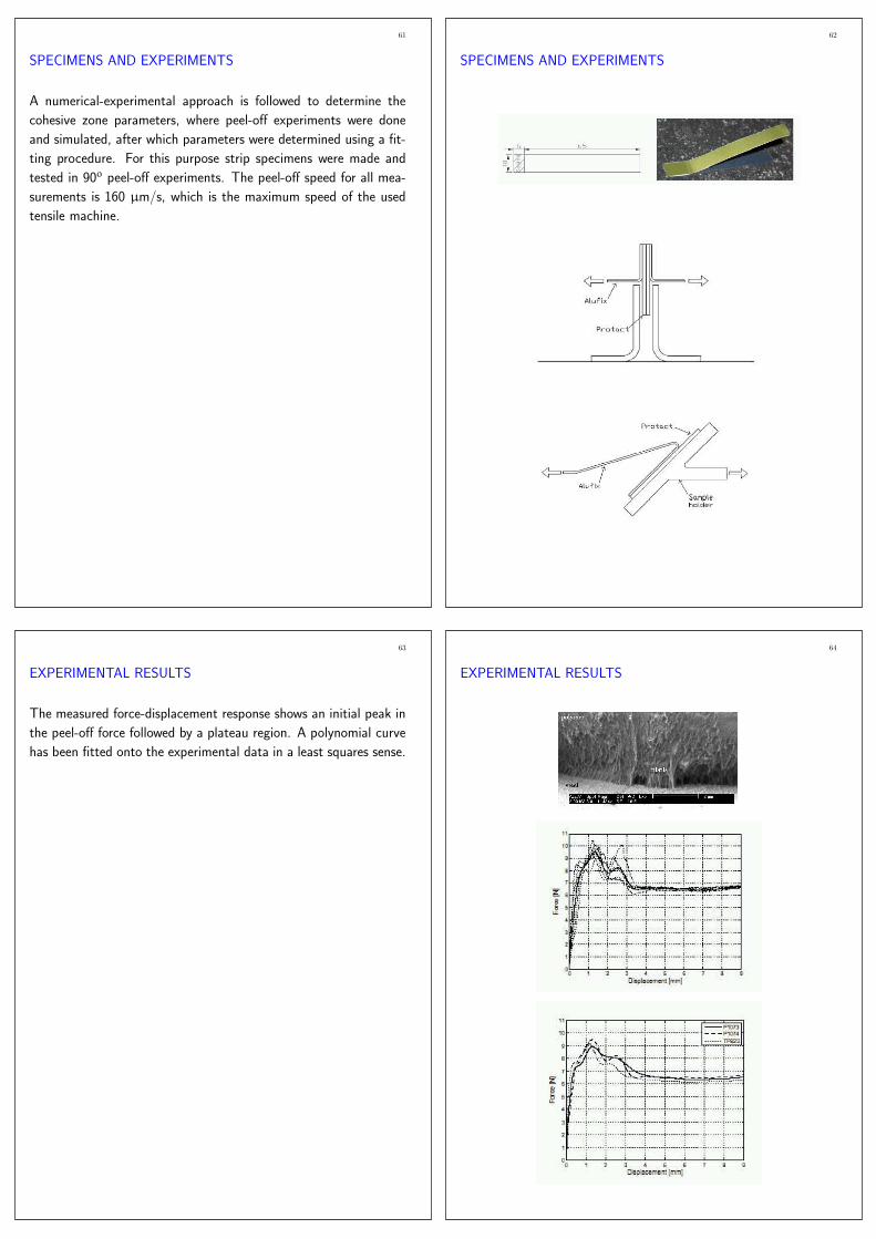
SPECIMENS AND EXPERIMENTS
A numerical-experimental approach is followed to determine the
cohesive zone parameters, where peel-off experiments were done
and simulated, after which parameters were determined using a fit-
ting procedure. For this purpose strip specimens were made and
tested in 90o peel-off experiments. The peel-off speed for all mea-
surements is 160 µm/s, which is the maximum speed of the used
tensile machine.
62
SPECIMENS AND EXPERIMENTS
63
EXPERIMENTAL RESULTS
The measured force-displacement response shows an initial peak in
the peel-off force followed by a plateau region. A polynomial curve
has been fitted onto the experimental data in a least squares sense.
64
EXPERIMENTAL RESULTS

65
PARAMETER IDENTIFICATION
To investigate the behavior of the EPOL closure, a finite element
model must been made, where an interface crack between alufix and
steel substrate is propagated to simulate the opening. The interface
crack is modeled with a cohesive zone element. The cohesive zone
model does not describe mode-mixity.
The characteristic length δ is measured from ESEM images,
recorded during the peel-off experiment. Although the accuracy
of the values can be doubted, it appeared that the sensitivity of
the value is not large. The potential φ is fitted onto the plateau
force value, which was measured and also simulated with the finite
element method using a model of the peel-off test.
A mesh sensitivity analysis is performed for the validation model.
The number of elements over the thickness of the aluminum foil was
chosen to be five, which appeared satisfactory. The number of el-
ement over the length of the strip is important because this also
includes the cohesive zone elements which are responsible for the
peel-off force. It appeared that using 200 elements was accurate
enough.
The parameter values are listed in the table for the three pro-
tact materials. Also the measured and simulated force-displacement
curves for P1073 are shown.
The peel-off specimens are also tested with a 135o peel-off load.
Using the fitted data from the 90o peel-off tests, these experiments
are also simulated and both results are shown in the figure for
P1073.
66
PARAMETER IDENTIFICATION
Protact φ [jm−2 Tmax [MPa] δ [µm]
P1073 170 19.5 3.2
P1074 213 11.7 6.7
TP823 162 19.9 3.0
P1073 : 90o P1073 : 135o
67
BURST PRESSURE EXPERIMENTS AND SIMULATION
The food sterilization process, where food is heated up for a specific
time at a temperature of 121o C, takes place inside a closed can.
During this process the pressure inside the can increases, which may
lead to EPOL burst. At Corus burst pressure experiments were done
at room temperature (20o C) and at sterilization temperature (121o
C). For all material systems, the alufix foil ruptured before failure of
the adhesion interface. At room temperature the maximum pressure
was 3.4 bar and at elevated temperature the maximum pressure
was 2.3 bar on average. This premature alufix failure prevented
the validation of the interface crack propagation model by burst
pressure simulations. To make some comparison, the deformation
of the protact rings were measured and used later for comparison
with numerical results.
Using the fitted cohesive zone parameters and other material
and geometric data, the burst pressure experiments were simulated.
Obviously no failure of the alufix could be implemented, so the
calculated burst maximum pressures at seal failure are far too high:
typically 3.1-4.3 bar. In the model, the residual stresses, strains
and hardening from the forming of the protact ring are taken into
account. The deformation of the protact ring could be compared
to the measured deformation and is shown in the figure for TP823.
Also a detail of the deformed cohesive layer is shown at a pressure
of 5.0 bar.
68
BURST PRESSURE EXPERIMENTS AND SIMULATION

69
OPENING EXPERIMENTS
The EPOL peel-off experiments are performed at Corus, where a
special EPOL peel-off tester is available. For P1073 protact, the
force-displacement curve is shown in the figure. The higher loads at
the start and the end of the experiment is caused by the geometry
of the seal.
70
OPENING EXPERIMENTS
71
OPENING SIMULATIONS
The EPOL peel-off model, is a three-dimensional FE model, which
uses the cohesive zones to describe the interfacial fibrillation of the
polymer layer during peeling. The model is reduced to one fourth
of the EPOL to diminish computing effort. This model reduction is
justified because the first half of the peel-off response of an EPOL
contains information about the initial peak force and the force in
the mid section, which is of most interest.
The deformation of P1073 protact is shown in the figures at
various stages of opening. Also the force-displacement curve is
depicted and compared to the experimental results.
72
OPENING SIMULATIONS

73
PARAMETER VARIATION (P1073)
Some parameters were given different values and the result of these
variations on the opening force-displacement are shown in the fig-
ures. In the first figure the width of the peal-off lid is varied. In
the second figure four simulations with different values for the seal
angle are presented. In the third figure three different seal widths
are used.
All simulatioons were done for the P1073 Protact material.
74
PARAMETER VARIATION (P1073)
lip width / seal angle / seal width
75
SOLDER JOINT FATIGUE
Solder joints provide electrical, thermal and mechanical continuity
in electronic packages. Today, miniaturization is the major driving
force in consumer electronics design and production. Efforts in
decreasing component dimensions have led to the development of
ball grid array (BGA) and flip chip packages, where solder balls are
employed. Following the legistative ban on lead (Pb), new soldr
alloys have been developed recently, which consist mainly of tin
(Sn).
76
SOLDER JOINT FATIGUE
SAC
top-Cu
bot-Cu
silicon
FR4
Y
Z X
1
-7.155e-05
4.536e-04
9.787e-04
1.504e-03
2.029e-03
2.554e-03
3.079e-03
3.604e-03
4.129e-03
4.654e-03
5.180e-03
lcase1
Total Equivalent Plastic Strain
Inc: 25
Time: 5.000e+00
Y
Z X
1
SnPb → SnAgCu

77
(THERMO)MECHANICAL CYCLING → FATIGUE LIFE
These solder balls are subjected to different types of loading:
• Thermal cycling due to repeated power switching evokes heat
related phenomena: the mismatch in the coefficient of thermal
expansion between the package components causes cyclic me-
chanical strains.
• As a result of the multi-phase nature of Sn based solder alloys
and the thermal anisotropy of β-Sn, internal stresses build up
in the solder.
• Cyclic thermo-mechanical loading evokes creep-fatigue damage
or creep rupture.
• Bending of the board induces shear and tensile stresses in the
solder joints.
The figure below shows a typical bump between two pads, where
thermal loading of the system leads to deformation and results in
plastic strains. Cyclic loading leads to fatigue damage and finally to
failure. Instead of using phenomenological laws like Manson-Coffin,
the fatigue damage is assessed with a cohesive zone approach.
78
(THERMO)MECHANICAL CYCLING → FATIGUE LIFE
SAC
top-Cu
bot-Cu
silicon
FR4
Y
Z X
1
-7.155e-05
4.536e-04
9.787e-04
1.504e-03
2.029e-03
2.554e-03
3.079e-03
3.604e-03
4.129e-03
4.654e-03
5.180e-03
lcase1
Total Equivalent Plastic Strain
Inc: 25
Time: 5.000e+00
Y
Z X
1
• Manson-Coffin (phenomenological, SN curve fitting)
∆εp = ε ′f (2Nf)
c → Nf = 12
(
∆εp
ε ′f
)1/c
– no micro-structure
– no damage initiation and propagation
⇒ no information for redesign bump shape or joint layout
better fatigue damage prediction needed
79
COHESIVE ZONE FOR FATIGUE FAILURE
The interaction between two associated points of a delaminating
interface in the solder joint is given by a traction-opening law :
Tα = Tα(∆α), where ∆α is the opening and Tα the traction, either
in normal (α = n) or tangential (α = t) direction. Because
deformations are small, there will be no problem relating to the
decomposition in normal and tangential direction. The relation
between traction and opening is taken to be linear. Damage is
introduced in the model by the degradation of the stiffness from a
given initial value to zero. The damage is quantified by a damage
variable Dα, which evolution during the loading history is given by
a damage evolution law. Its initial value is theoretically zero and its
final value at complete failure is one. The initial stiffness kα has
to be taken large enough to prevent any influence of the cohesive
zone layer, when there is no damage. Obviously, this initial value is
reversely related to the thickness of the cohesive zone, approaching
infinity, when this thickness is zero. The damage evolution law will
prevent damage growth, when the absolute value of the traction is
below the fatigue limit σf.
80
COHESIVE ZONE FOR FATIGUE FAILURE
Tα = kα(1 − Dα)∆α
Dα = cα|∆α| (1 − Dα + r)m
⟨
|Tα|
1 − Dα
− σf
⟩
kα MPa/mm initial stiffness
cα mm/N damage growth coeff.
r - coefficient
m - exponent
σf MPa fatigue limit
−5 0 5 10 15 20x 10−5
−400
−300
−200
−100
0
100
200
300
400
∆n [mm]
T n [M
Pa]
−2 −1 0 1 2x 10⁻⁴
−150
−100
−50
0
50
100
150
∆t [mm]
T t [M
Pa]
81
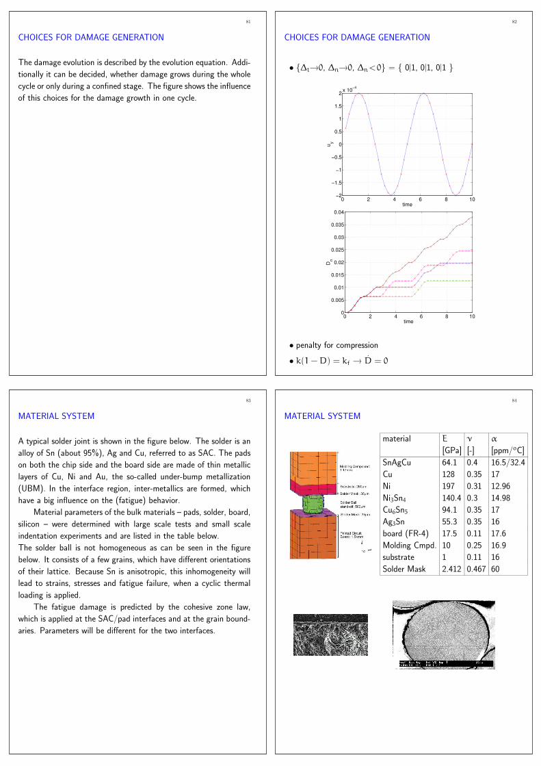
CHOICES FOR DAMAGE GENERATION
The damage evolution is described by the evolution equation. Addi-
tionally it can be decided, whether damage grows during the whole
cycle or only during a confined stage. The figure shows the influence
of this choices for the damage growth in one cycle.
82
CHOICES FOR DAMAGE GENERATION
• {∆t→0, ∆n→0, ∆n<0} = { 0|1, 0|1, 0|1 }
0 2 4 6 8 10−2
−1.5
−1
−0.5
0
0.5
1
1.5
2 x 10⁻⁴
time
u y
0 2 4 6 8 100
0.005
0.01
0.015
0.02
0.025
0.03
0.035
0.04
timeD n
• penalty for compression
• k(1 − D) = kf → D = 0
83
MATERIAL SYSTEM
A typical solder joint is shown in the figure below. The solder is an
alloy of Sn (about 95%), Ag and Cu, referred to as SAC. The pads
on both the chip side and the board side are made of thin metallic
layers of Cu, Ni and Au, the so-called under-bump metallization
(UBM). In the interface region, inter-metallics are formed, which
have a big influence on the (fatigue) behavior.
Material parameters of the bulk materials – pads, solder, board,
silicon – were determined with large scale tests and small scale
indentation experiments and are listed in the table below.
The solder ball is not homogeneous as can be seen in the figure
below. It consists of a few grains, which have different orientations
of their lattice. Because Sn is anisotropic, this inhomogeneity will
lead to strains, stresses and fatigue failure, when a cyclic thermal
loading is applied.
The fatigue damage is predicted by the cohesive zone law,
which is applied at the SAC/pad interfaces and at the grain bound-
aries. Parameters will be different for the two interfaces.
84
MATERIAL SYSTEM
material E ν α
[GPa] [-] [ppm/oC]
SnAgCu 64.1 0.4 16.5/32.4
Cu 128 0.35 17
Ni 197 0.31 12.96
Ni3Sn4 140.4 0.3 14.98
Cu6Sn5 94.1 0.35 17
Ag3Sn 55.3 0.35 16
board (FR-4) 17.5 0.11 17.6
Molding Cmpd. 10 0.25 16.9
substrate 1 0.11 16
Solder Mask 2.412 0.467 60

85
SPECIMENS AND EXPERIMENTS
To test the fatigue behavior of the interface, tensile and shear spec-
imens were made. Both tensile and shear experiments/simulations
were done, using a micro tensile stage, mounted in an ESEM, to
allow for observation of the interface.
To investigate the degradation of the inter-granular interface
in the bulk solder, unconstrained test specimens were subjected to
a cyclic thermal load. The resulting loss of interface integrity was
assessed by measuring the Young’s modulus after a certain number
of loading cycles.
86
SPECIMENS AND EXPERIMENTS
mechanical cycling → reaction force/area (nr. cycles)
SEM, OIM, misorient.
500 cycles
−40 < T < 125 oC
thermal cycling → macroscopic stiffness
87
PARAMETER IDENTIFICATION : SAC/PAD : MECHANICAL
Assessment of the parameters in the damage evolution law has
been done with an experimental-numerical approach, where fatigue
failure data from experiments were confronted with simulation data.
The tensile and shear experiments have been modeled with the finite
element method and these models have been subjected to a cyclic
mechanical load.
The parameter identification procedure resulted in values for
the cz-parameters, which are listed in the table below. Experimental
and numerical results are also shown in the figure as stress against
the number of loading cycles.
Also the bulk solder has been modeled and subjected to the
cyclic thermal load from the experiments. The cz-parameters for the
inter-granular interfaces were fitted such that the stiffness reduction
of the model was the same as that of the experiments.
88
PARAMETER IDENTIFICATION : SAC/PAD : MECHANICAL
cz k c m r
[N/m3] [m/N] [-] [-]
SAC/pad n 8.79e8 68000 3.160 1e-6
SAC/pad t 3.21e8 47000 3.135 4e-5

89
PARAMETER IDENTIFICATION : SAC GR.B. : THERMAL
The parameters of the intergranular cohesive zones can not be de-
termined by mechanical testing. Instead a thin sheet of solder ma-
terial is loaded with a cyclic temperature. Due to the anisotropic
thermal and mechanical properties of the various grains, stresses in
the material occur, which constitute load on the interfaces. This
cyclic load results in damage growth. The damage as a function of
the number of cycles is characterised by the global Young’s modu-
lus of the material. Confronting experimental data with numerical
results allows the parameter identification.
90
PARAMETER IDENTIFICATION : SAC GR.B. : THERMAL
cz k c m r
[N/m3] [m/N] [-] [-]
SAC grain.bndy. n 6.40e8 42000 2.940 0
SAC grain.bndy. t 2.28e8 42000 2.940 0
91
SOLDER BALL FATIGUE FAILURE
Having determined all parameters of bulk materials and cohesive
zones, the damage evolution in a bump could be analyzed. The fig-
ure below shows a two-dimensional plane strain bump/pad model.
Boundary conditions are very important for the fatigue life, so dif-
ferent load cases have been studied.
The damage in the solder ball and the solder/pad interface is
shown in the next figures after 250 and 1000 cycles, for the three
selected boundary conditions. The deformation is enlarged 5×. It
is clearly seen that the bump is completely detached from the pad
after 1000 cycles.
92
SOLDER BALL FATIGUE FAILURE
PSfrag replacements
cz1cz2
cz3cz4
PSfrag replacements
X
Y
Z
1
X
Y
Z
1
X
Y
Z
1
X
Y
Z
1
X
Y
Z
1
X
Y
Z
1

93
SOLDER BALL FATIGUE FAILURE
The simulation results are validated using an experimental analysis
of BGA packages under thermal cycling and thermal shock loading.
All slice models are computed separately for both types of loading,
until N = 1000 cycles. The numerical results are then extrapolated
to N = 5000. A critical effective damage value Deff is defined
to predict the number of cycles to failure (ncf), that adequately
reproduces the experimental failure distributions provided by the
industry.
First, all slice models were computed without any defects, rep-
resenting a theoretical case. Then, defects were introduced in the
mesh, as they were statistically determined. Last, a data set con-
sisting of good (45 %) and defective balls (55 %) is constructed.
The figure shows that, with a critical damage level for failure
equal to Dcriteff = 0.87, a good agreement between the statistically
constructed data set and the experimental data is obtained. The
fatigue life of long living (N > 5000) solder balls is overestimated.
This seems logical due to the fact that, as mentioned previously,
the cross-sectional defect analysis hides many defects, yielding too
optimistic results (45 % of all solder balls were defect-free). In
reality, more defects have to be inserted into the slice models.
94
SOLDER BALL FATIGUE FAILURE
cycling shock
95
PARAMETER VARIATION
Although many parameters could obviously be varied, the behavior
of various solder geometries and grain distributions was investigated
when they were subjected to cyclic mechanical loading. The solder
joint is placed between chip and board as is shown in the figure.
From these simulations the following conclusions could be drawn:
• As the contact angle α decreases, cross-sectional averages of
plastic strain and Von Mises stress values increase.
• A horizontal grain boundary becomes more critical when the
contact angle increases. However, the highest stress is found at
bump/pad interface.
• A vertical grain boundary may play a crucial role in solder joint
reliability, which becomes more pronounced as the grain bound-
ary area increases.
• Vertical grain boundaries that touch the bump/pad interface
have the highest stress level under thermal loading and there-
fore constitute a possible crack initiation path starting from the
bump/pad interface.
96
PARAMETER VARIATION
• α ↓ → (εp, σvm)crossection ↑• α ↑ → hor. grain boundary more critical
• gr.bnd.area ↑ → vert. grain boundary more critical
• vert. grain bnd’s touching bump/pad →highest stress level

97
END
98
END