Atmospheric Power Law Behavior James Duncan

Philip Sura

The Study of Extreme Events

• Extreme climatic events are weather phenomena that occupy the tails of a dataset’s probability density function (PDF).

• While it understood that the PDFs of atmospheric phenomena are non-Gaussian, the exact shape/distribution of these tails are not fully understood.

• Analysis of recent observational studies have shown that many atmospheric variables follow a power law distribution in the tails of their distribution.

Mathematically, a power law probability distribution of quantity x may be written as:

Where α is the exponent or scaling parameter and C is the normalization constant.

Stochastic theory asserts that power law distributions should exist in the tails of distributions.

What is a Power Law Distribution?

€

p(x) = Cxmin−α

[Newmans et al. 1986]

Construction of the Power Law Algorithm

• Calculate a lower bound xmin and some scaling parameter α of our power law distribution.

• Calculate the goodness of fit between the empirical data and the power law. Make preliminary conclusion based upon resulting p-value.

• Perform a likelihood ratio test comparing competing hypothesis/distribution fits.

Estimating Lower Bound on Power Law Behavior

• For the case of empirical data, if the data is to follow a power-law distribution, it does so only above some lower bound xmin.

• To find our lower-bound, xmin, we employ the Kolmogorov-Smirnov or KS Statistic which the maximum difference between the CDF of the observed data and the CDF of the estimated power law distribution.

€

D = maxx≥xmin

| F(x) − P(x) |[Press et al. 1986]

Estimating the Scaling Parameter

• An accurate estimate of is dependent upon an accurate estimate of our lower bound, xmin.

• To do so, we employ the “method of maximum likelihood” given by:

€

ˆ α =1+ n lnx i

xmini=1

n

∑ ⎡

⎣ ⎢

⎤

⎦ ⎥

−1

• Employ the use of a goodness of fit test which will measure and analyze the KS distance of our power law distribution with that of other synthetically derived power law distributions.

• From the goodness of fit test, we are able to derive a “p-value” which expresses the probability that the estimated power law distribution is a good fit to the observed data.

Significance Testing

About the Data

• Daily weather observations from the southeastern United States (AL, FL, GA, NC, SC) spanning 1948-2009.

• Data includes minimum and maximum temperatures, and daily precipitation amounts.

• Mean annual cycle has been removed from the data.

Motivation for Power Law

Skewness Kurtosis

€

γ=μ3

σ 3

€

κ =μ4

σ 4

− 3[Press et al. 1986]

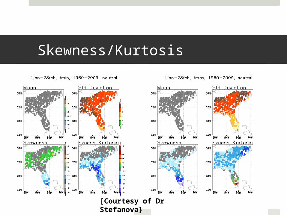
Skewness/Kurtosis

[Courtesy of Dr Stefanova}

Ft Lauderdale

α xmin ppower pgauss

Positive 23.53

2.44 .118 0.00

Negative

7.64 2.98 .22 .037

α xmin ppower pgauss

Positive

10.98 2.62 .498 .602

Negative

5.76 3.16 .364 .007

Negative Kurtosis, Negative Skew Positive Kurtosis, Negative Skew

Pensacola

α xmin ppower pgauss

Positive 14.7 2.44 .0204 0.00

Negative 7.68 3.16 .928 .076

α xmin ppower pgauss

Positive 14.7 2.44 .0204 0.00

Negative 7.68 3.16 .928 .076

Negative Kurtosis, Positive Skew Negative Kurtosis, Negative Skew

Future Work

• Further examine power law distributions in the physical world.

• Analyze these distributions during years of distinction: • El Niño and La Niña years

• Seasonal trends

• Historically active or tranquil hurricane seasons

• Years of intense drought or flooding events

Questions?

References:Clauset, A., C. R. Shalizi, and M. E. J. Newman, Power-law distributions in empirical data, SIAM Review, 51, 661-703, 2009.Newman, M. E. J., Power laws, Pareto distributions and Zipf’s law, Contemporary Physics, 46(5), 323-351, 2005.Press, W. H., B. P. Flannery, S. A. Teukolsky, and W. T. Vetterling, Numerical Recipes: The Art of Scientific Computing, 1st ed., 818 pp., Cambridge University Press, 1986.