coal mining and human wellbeing: a case-study in …...coal mining and human wellbeing: a case-study...

This file is part of the following reference:

Li, Qian (2016) Coal mining and human wellbeing: a

case-study in Shanxi, China. PhD thesis, James Cook

University.

Access to this file is available from:

http://researchonline.jcu.edu.au/47252/

The author has certified to JCU that they have made a reasonable effort to gain

permission and acknowledge the owner of any third party copyright material

included in this document. If you believe that this is not the case, please contact

[email protected] and quote


ResearchOnline@JCU


mailto:[email protected]


Coal mining and human wellbeing: A case-study in Shanxi, China

Thesis submitted by

Qian Li

In April 2016 For the degree of Doctor Philosophy

James Cook University

Townsville Queensland 4811

Australia

i

Statement of Contribution of Others

Financial support

• Graduate Research School, James Cook University

• Chinese Scholarship Council (CSC)

• College of Science and Engineering (formerly the School of Earth and Environmental Sciences), James Cook University

• College of Business, Law and Governance (formerly School of Business), James Cook University

Thesis Committee

• Associate Professor David King

• Professor Natalie Stoeckl

• Associate Professor Emma Gyuris

Intellectual support

Research design

Professor Natalie Stoeckl

Questionnaire design




Data collection

6 Research assistants 1

Data analysis and statistical support


1 Research assistants recruited from Shuozhou, Linfen and Yangquan were university students living or studying in the case-study areas and spoke local dialect. They were responsible for interviewing the respondents and filling out questionnaire.

ii

• Dr Rabiul Beg

Editorial support




Permits

Research associated with this thesis complies with current laws of Australia and all

permits necessary for the project obtained (JCU Human Ethics H5094).

iii

Acknowledgements

I felt lucky in the beginning of the journey just because of the fact that I was here to start

my journey. At the end, when I look back, I feeI blessed. Without the loving and

supportive network I have, I would not have made such a significant progress, and this

journey could not have been so amazing.

My gratitude to my outstanding supervisors is beyond words. First, thanks to Associate

Professor David King, I would not have had this opportunity without his support. He

helped me with all the major or trivial issues from the first day until the last with lots of

patience and trust. He provided valuable guidance for my research and detailed

feedback, kept me motivated and made sure my work went smoothly.

Professor Natalie Stoeckl, she spared no efforts and time to help me with every stage of

my PhD. She always inspired me with wonderful ideas, for the structure and details of

my research. The notes from her to help me understand her ideas accumulated into a

pile. I am amazed by her ability to make everything so interesting. She always found a

way to make me feel confident and passionate about my research. I am indebted to her

for her kindness, patience, and encouragement to me.

Associate Professor Emma Gyuris offered valuable ideas and support to my writing,

presentation etc. I was impressed with her diligence, rigorous thinking and attention to

the details, which improved my work dramatically.

I could not image what the journey would have been like without Emma Ryan, my

dearest friend. The friendship with her is one of the best things from this journey, which

has significant meaning to me. We spent so much time in and outside University and

shared numerous unforgettable moments. She accompanied me through my ups and

downs, and always offered help before I even asked for it. Many thanks to the lovely

girls from the lunch group as well as my office mate Astrid Vaschette. They make every

ordinary working day cheerful.

I would like to thank everyone who participated in the fieldwork, and lots of friends,

such as Cheryl Fernandez, Rie Hagihara and Meen Hong, who offered me practical advice.

iv

I am deeply grateful to my family. As usual, they shared all my struggling, growth and

happiness, protected me from any distractions from my PhD and supported me

unconditionally.

v

Abstract

Coal has been an essential source of energy that has fuelled economic growth and

development throughout modern history. Its use has delivered astonishing

developments in human living standards and wellbeing. Coal is the most affordable and

widely available source of energy. It is particularly essential for developing countries,

such as China, as it helps deliver economical and stable electricity to underpin economic

growth and poverty alleviation. That said, environmental problems associated with coal,

such as human-enhanced greenhouse effects generated when coal is burned are of

concern.

For host (mining) communities, coal mining seems to also be a two-edged sword. Coal

resource development, for example, can bring numerous jobs, can increase household

incomes and can generate revenue for governments, which is significant for regional

development. But numerous negative impacts have been documented; coal mining can

adversely affect natural capital (environment), human capital, social capital, institutional

capital and the economy (e.g. through inflation). These ‘capitals’ all contribute to human

wellbeing; so the impacts of mining on human wellbeing are complex and multifaceted.

Some impacts, such as mining revenues, are tangible, likely positive, and can be easily

observed and quantified from market transactions. In contrast, other impacts, on the

environment, culture, and society, are often intangible are thus much less easily

quantified or observed.

Existing mining impact assessment processes, such as environmental/social/economic

impact assessment, and assessments of eco-compensation for mining, struggle to

quantify the numerous non-market impacts of mining; they thus struggle to provide data

to defensibly assess trade-offs between the benefits and costs of mining that takes

account of all tangible and intangible impacts on host communities. This difficulty results,

partly, from the fact that currently available methods (mostly traditional economic non-

market valuation techniques) for assessing intangible impacts are on occasion

inadequate – particularly when assessing numerous simultaneous and inter-related

impacts. The life satisfaction (LS) approach, shows advantages over other non-market

vi

valuation methods, and has been successfully used to assess a range of non-market

goods, but it has not yet been used to measure the impacts of mining.

This study aims to assess the impacts of coal mining on LS – associated with the more

general term ‘human wellbeing’, which includes objective and subjectice dimensions.

Specifically, it uses insights from the wellbeing literature and from the LS approach to

quantify and compare multiple impacts of coal mining; and it assesses the trade-off

between benefits (mostly monetary – e.g. through income) and costs (numerous, often

intangible) of coal mining on host communities. In doing so, it offers insights into how

coal mining affects a range of wellbeing factors or life domains. It also provides insights

about the net impacts of mining, about who benefits most/least from coal mining and

about how one might target policy to compensate those who do not perceive a net

benefit. It thus identifies policy priorities to help mitigate the negative and enhance the

positive impacts of coal mining on human wellbeing.

This study focusses on 3 major research questions, each of which is directly linked to an

identified research gap:

1. How does coal mining affect people’s subjective perceptions of different

wellbeing factors? This includes the importance attached to each wellbeing

factor, satisfaction with each factor, and people’s perception about the impacts

of coal mining on these factors.

2. Does information about the impacts of coal mining derived from subjective

assessments of wellbeing convey the same message about the impacts of coal

mining as ‘objective’ measures of wellbeing?

3. Is it possible to quantify the net impacts of coal mining (on broad ‘domains’ of

life and on the overall wellbeing of host communities) and to determine how

much should, in principle, be paid ‘in compensation’ to those who are, overall,

impacted negatively?

Shanxi province, the most important coal producer in China, was selected as the case-

study region. Within Shanxi, 5 types of case-study areas, including rural areas with coal

mining (Rural With), rural areas close to coal mining (Rural Close), urban areas close to

coal mining (Urban Close), urban areas far from coal mining (Urban Far) and rural areas

vii

far from coal mining (Rural Far) were selected for focus – providing insights from a cross-

section of people with differential exposure to coal mining.

A comprehensive set of data on wellbeing was not available in the case-study areas.

Therefore, questionnaire surveys were used to collect data on 29 different factors

known (from the literature) to affect wellbeing. Residents were asked to indicate how

important they thought each factor was to their overall wellbeing, how satisfied they

were with each, and how they thought coal mining was (or could) impact those factors.

They were also asked about their satisfaction with life overall, and to provide some basic

sociodemographic information. ‘Objective’ indicators of air quality were collected at

each location. A total of 542 valid questionnaires were collected.

Responses to questions about satisfaction (with factors), importance (of factors) and

perceptions (of the impacts of coal mining on those factors) were examined separately,

and 2 indices, one combining satisfaction and importance (Index of Dis-Satisfaction –

IDS), and the other combining satisfaction and perceptions of impacts (Index of Dis-

Satisfaction and Negative Impacts – IDSNI) were constructed. Indicators related to

health and relationship were deemed – by the entire sample, and by each sub-sample –

to be the most important factors; these were also the factors with which people from

all the study areas were most satisfied. People living in coal mining areas were most

dissatisfied with factors relating to environmental quality (air quality and water safety)

and the economy (real estate prices and inflation), while people in non-coal mining areas

were most dissatisfied with factors only relating to the economy. People from all the

study regions expressed most concern about the impacts of mining on the factors

relating to the environment and health. Both IDS and IDSNI indicate that in coal mining

areas both environmental issues and economic issues were of high priority, and

environmental issues were paramount. IDS indicates that in non-coal mining areas,

economic issues and social issues (the quality of government, education and property

safety) were of most concern.

Available objective wellbeing indicators were regressed against subjective wellbeing

indicators, controlling for sociodemographic factors (such as age, family size and gender).

The relationships between some subjective and objective indicators were statistically

viii

significant (e.g. higher levels of family income were associated with higher satisfaction

with family income, and higher levels of PM10 were associated with lower levels of

satisfaction with air quality), but some were not (the objective indicators of housing

conditions did not always predict satisfaction with housing). These relationships were

always mediated by sociodemographic variables indicating that subjective and objective

indicators are not ‘perfect’ substitutes for each other. These results indicate that it is

both possible and necessary to use subjective indicators of wellbeing in addition to

traditionally used objective indicators to inform public policy in coal mining regions.

Moreover, this study demonstrates approaches that can be used to explore the

relationship between objective and subjective indicators which could be used to inform

future policy makers about when it is most/least appropriate to use only objective or

only subjective indicators.

Using principal component analysis, the 29 wellbeing factors were collapsed into 6 life

domains: human capital, economy, social capital, institutional capital, living conditions

and natural environment. Factor scores relating to each domain were retained for use

as dependent variables in regression models. The sample was divided in two (rural and

urban), and variables denoting proximity to coal mining and sociodemographic factors

were included as regressors so that the impacts of mining on satisfaction with life

domains and on LS could be assessed while controlling for other potentially confounding

factors. Factor scores from each domain and measures of global life satisfaction were

each regressed against numerous factors known to influence subjective assessments of

wellbeing.

Urban residents were found to be relatively insensitive to the impacts of coal mining.

Although people living in places with or close to coal mines in rural areas (“Rural With”

and “Rural Close”) had statistically significant lower levels of satisfaction across multiple

life domains (the natural environment, the economy and society) than those living

further away from mines, they were, however, more satisfied with their living conditions.

After controlling for confounding sociodemographic factors, the analysis revealed that

rural residents living in areas adjacent to coal mines had experienced lower levels of

satisfaction with life overall than those living more than 10km away from mines. It was

possible to use coefficients from the LS model to infer that a similar ‘loss’ of life

ix

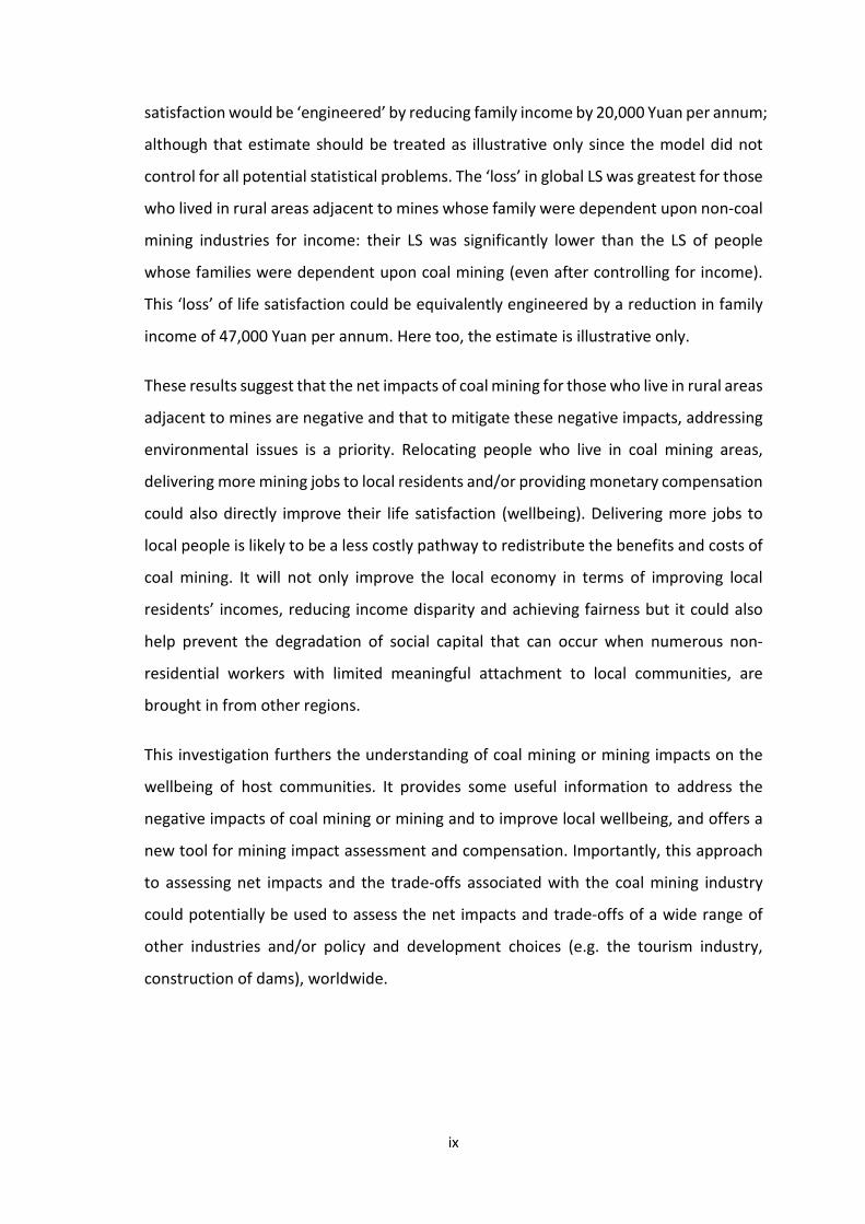
satisfaction would be ‘engineered’ by reducing family income by 20,000 Yuan per annum;

although that estimate should be treated as illustrative only since the model did not

control for all potential statistical problems. The ‘loss’ in global LS was greatest for those

who lived in rural areas adjacent to mines whose family were dependent upon non-coal

mining industries for income: their LS was significantly lower than the LS of people

whose families were dependent upon coal mining (even after controlling for income).

This ‘loss’ of life satisfaction could be equivalently engineered by a reduction in family

income of 47,000 Yuan per annum. Here too, the estimate is illustrative only.

These results suggest that the net impacts of coal mining for those who live in rural areas

adjacent to mines are negative and that to mitigate these negative impacts, addressing

environmental issues is a priority. Relocating people who live in coal mining areas,

delivering more mining jobs to local residents and/or providing monetary compensation

could also directly improve their life satisfaction (wellbeing). Delivering more jobs to

local people is likely to be a less costly pathway to redistribute the benefits and costs of

coal mining. It will not only improve the local economy in terms of improving local

residents’ incomes, reducing income disparity and achieving fairness but it could also

help prevent the degradation of social capital that can occur when numerous non-

residential workers with limited meaningful attachment to local communities, are

brought in from other regions.

This investigation furthers the understanding of coal mining or mining impacts on the

wellbeing of host communities. It provides some useful information to address the

negative impacts of coal mining or mining and to improve local wellbeing, and offers a

new tool for mining impact assessment and compensation. Importantly, this approach

to assessing net impacts and the trade-offs associated with the coal mining industry

could potentially be used to assess the net impacts and trade-offs of a wide range of

other industries and/or policy and development choices (e.g. the tourism industry,

construction of dams), worldwide.

x

Table of Contents 1. CHAPTER 1 INTRODUCTION ................................................................................................. 2

1.1 Introduction ...................................................................................................................3

1.2 The benefits of mining and coal mining .........................................................................5

1.3 Downsides of mining or coal mining ..............................................................................8

1.3.1 Coal mining and the natural environment ............................................................ 9

1.3.2 Mining and economic growth ............................................................................. 10

1.3.3 Mining and human capital .................................................................................. 12

1.3.4 Mining and social capital ..................................................................................... 12

1.3.5 Mining and institutional capital (governance) .................................................... 14

1.4 The current policy focus on and research gaps of coal mining’s impacts on host communities............................................................................................................................ 15

1.5 Structure of this thesis ................................................................................................ 17

2. CHAPTER 2 LITERATURE REVIEW ....................................................................................... 20

2.1 Introduction ................................................................................................................ 21

2.2 Approaches to assessing the impacts of coal mining .................................................. 21

2.2.1 Traditional approaches to assessing the impacts of coal mining........................ 22

2.2.2 Assessing the value of non-market goods .......................................................... 27

2.3 Human wellbeing ........................................................................................................ 32

2.3.1 The definition and dimension of human wellbeing ............................................ 33

2.3.2 Factors that contribute to human wellbeing ...................................................... 36

2.3.3 Wellbeing indicators used in the literature ........................................................ 43

2.4 Coal mining and human wellbeing .............................................................................. 45

2.5 Literature examining human wellbeing in coal mining regions .................................. 48

2.5.1 Lack of holistic investigations into a range of wellbeing factors and the trade-off between benefits and costs ................................................................................................ 48

2.5.2 Lack of subjective wellbeing measurement ........................................................ 49

2.5.3 Lack of importance weighting ............................................................................. 51

2.5.4 Lack of investigation into perception of local residents about impacts of mining ………………………………………………………………………………………………………………………..52

2.5.5 Lack of the empirical alignment between subjective and objective wellbeing measurement ...................................................................................................................... 54

2.5.6 Lack of comparison of different case-study areas characterized by different intensities of coal mining .................................................................................................... 55

2.6 Summary: research gaps and questions ..................................................................... 56

xi

3. CHAPTER 3 THE CASE-STUDY AREA AND DATA COLLECTION METHODS ............................ 61

3.1 Introduction ................................................................................................................ 62

3.2 Coal mining in China .................................................................................................... 62

3.3 Shanxi province ........................................................................................................... 64

3.4 Questionnaire Development ....................................................................................... 67

3.4.1 Questions for the questionnaire ......................................................................... 68

3.4.2 Collection of data relating to objective wellbeing .............................................. 79

3.4.3 Wording and sequencing questions .................................................................... 79

3.5 Data collection ............................................................................................................ 82

3.5.1 Sampling framework ........................................................................................... 82

3.5.2 Survey implementation ....................................................................................... 85

3.5.3 Controlling survey errors ..................................................................................... 87

3.6 Sample overview ......................................................................................................... 88

3.7 Conclusion ................................................................................................................... 92

4. CHAPTER 4 SATISFACTION WITH, IMPORTANCE OF AND PERCEIVED IMPACTS OF COAL MINING ON WELLBEING FACTORS .............................................................................................. 94

4.1 Introduction ................................................................................................................ 96

4.2 Analytical method ....................................................................................................... 97

4.2.1 Sub-research questions 1-3s ............................................................................... 97

4.2.2 Sub-research question 4 ..................................................................................... 98

4.2.3 Sub-research question 5 ..................................................................................... 99

4.3 Results ....................................................................................................................... 100

4.3.1 Sub-research question 1: the importance of wellbeing factors ........................ 100

4.3.2 Sub-research question 2: satisfaction with different wellbeing factors ........... 102

4.3.3 Sub-research question 3: perceptions of the impacts of coal mining on wellbeing factors…………………………………………………………………………………………………………………………..106

4.3.4 Research question 4: the relationship between satisfaction and importance . 110

4.3.5 Research question 5: the relationship between satisfaction level and the impact of coal mining .................................................................................................................... 115

4.4 Conclusion and discussion ........................................................................................ 119

4.4.1 Implications for policy makers .......................................................................... 126

4.4.2 Methodological contribution ............................................................................ 126

5. CHAPTER 5 EXPLORING THE RELATIONSHIP BETWEEN OBJECTIVE AND SUBJECTIVE INDICATORS OF WELLBEING ..................................................................................................... 128

5.1 Introduction .............................................................................................................. 130

xii

5.2 Analytical method ..................................................................................................... 131

5.3 Results ....................................................................................................................... 135

5.3.1 The relationship between objective and subjective indicators relating to family income............................................................................................................................... 135

5.3.2 The relationship between objective and subjective indicators relating to air quality................................................................................................................................138

5.3.3 The relationship between objective and subjective indicators relating to housing..............................................................................................................................141

5.3.4 The relationship between objective and subjective indicators relating to education .......................................................................................................................... 145




5.4.3 Implications for future studies .......................................................................... 154

6. CHAPTER 6 IMPACTS OF COAL MINING ON SUBJECTIVE WELLBEING: USING THE LIFE SATISFACTION APPROACH ........................................................................................................ 156

6.1 Introduction .............................................................................................................. 159

6.2 Analytical method ..................................................................................................... 160

6.2.1 Assessing the impact of coal mining on different life domains ........................ 160

6.2.2 Assessing the impacts of coal mining on global life satisfaction ...................... 165

6.3 Results ....................................................................................................................... 168

6.3.1 Determinants of satisfaction with life domains ................................................ 168

6.3.2 Impacts of coal mining on global life satisfaction ............................................. 174




6.4.3 Implications for future studies .......................................................................... 195

7. CHAPTER 7 SYNTHESIS AND DISCUSSION ........................................................................ 198

7.1 Introduction .............................................................................................................. 199

7.2 Overview of the thesis .............................................................................................. 199

7.3 Empirical contributions ............................................................................................. 209

7.4 Discussion of empirical findings ................................................................................ 212

7.5 Methodological contributions and implications for policy makers or practitioners 216

7.5.1 Methodological contributions and insights for monitoring/ measuring wellbeing ........................................................................................................................... 216

7.5.2 Methodological contributions to the impact assessment literature ................ 218

xiii

7.6 Implications for future research ............................................................................... 220

7.7 Concluding comments ............................................................................................... 222

References................................................................................................................................. 223

Appendix A: Questionnaire ....................................................................................................... 241

Appendix B: Comparison of income between the (coal) mining industry and other industries ................................................................................................................................................... 249

Appendix C: The relationship between objective and subjective wellbeing indicators ........... 251

Appendix D: Ordinal regression – Impacts of coal mining on subjective wellbeing ................. 260

xiv

List of Tables

Table 3.1 Area and population of case-study areas (2013) ....................................................... 66

Table 3.2 Output for major industrial products above designed size (2013) ............................ 67

Table 3.3 Refined terms for subjective/objective wellbeing ...................................................... 68

Table 3.4 Selected wellbeing factors according to the literature .............................................. 72

Table 3.5 Scales used in the questionnaire ................................................................................. 77

Table 3.6 Sociodemographic variables found to be significant in explaining overall life

satisfaction .................................................................................................................................. 78

Table 3.7 Criteria for selecting sampling sites that represent different intensities of coal mining

..................................................................................................................................................... 84

Table 3.8 Sampling of study regions .......................................................................................... 87

Table 3.9 Sample information .................................................................................................... 90

Table 4.1 IDS for individual factors, arranged from highest to lowest score for each type of

study region .............................................................................................................................. 113

Table 4.2 IDSNI for individual factors, arranged from highest to lowest score for 3 types of

study region .............................................................................................................................. 118

Table 4.3 Summary of findings .................................................................................................. 119

Table 5.1 OLS regression results – with dependent variable being subjective measures of

respondent satisfaction with income ....................................................................................... 137


respondent satisfaction with air quality ................................................................................... 140


respondent satisfaction with housing ....................................................................................... 144

Table 6.1 Life domains created using PCA on satisfaction scores for the 29 wellbeing factors,

with factor loadings .................................................................................................................. 169

Table 6.2 Results from OLS regression of factor scores (relating to satisfaction with different

life domains) and other variables (sociodemographic factors and proximity to coal mines) .. 172

Table 6.3 Synthesis of tests for statistically significantly differences in model coefficients for

the urban/rural models ............................................................................................................. 173

Table 6.4 Comparison of average life satisfaction scores between sample in this study and

other studies ............................................................................................................................. 178

Table 6.5 Result from OLS regression of global life satisfaction and other variables

(sociodemographic factors and proximity to coal mines) ........................................................ 179

xv

List of Figures

Figure 1.1 Coal production all over the world ............................................................................. 7

Figure 2.1 Full World Model of the Ecological Economic System .............................................. 37

Figure 2.2 Framework for OECD wellbeing indicators ............................................................... 44

Figure 2.3 Limits to the economic growth ................................................................................. 46

Figure 3.1 Map of Shanxi province ............................................................................................. 66

Figure 3.2 Different types of study region ................................................................................. 85

Figure 4.1 Mean scores relating to perceived importance of factors to overall wellbeing

displayed from most important to most unimportant ............................................................. 101

Figure 4.2 Mean scores relating to perceived importance of factors to overall wellbeing by

study region .............................................................................................................................. 102

Figure 4.3 Mean scores relating to satisfaction with wellbeing factors displayed from most

dissatisfied to most satisfied ..................................................................................................... 103

Figure 4.4 Mean scores relating to satisfaction with wellbeing factors by study region ........ 104

Figure 4.5 Mean scores relating to perceived impact of coal mining on wellbeing factors

displayed from most negative to most positive impact ........................................................... 107

Figure 4.6 Mean scores relating to perceived impact of coal mining on wellbeing factors by

study region .............................................................................................................................. 108

Figure 4.7 Travelling long distance to get water ...................................................................... 109

Figure 4.8 A little “white dog” in a village with coal mining .................................................... 110

Figure 4.9 A little dog in a city close to coal mining ................................................................. 110

Figure 4.10 Mean scores relating to satisfaction with and importance of wellbeing factors .. 111

Figure 4.11 The relationship between mean scores relating to dissatisfaction and importance

................................................................................................................................................... 112

Figure 4.12 Mean scores relating to satisfaction with and perceived impact of coal mining on

wellbeing factors ....................................................................................................................... 115

Figure 4.13 The relationship between mean scores relating to dissatisfaction and perceived

impact of coal mining ................................................................................................................ 117

Figure 4.14 Heavy truck carrying coal through the middle of a village .................................... 123

Figure 5.1 Annual family income and satisfaction level of income by study region ................ 136

Figure 5.2 Concentration of PM 10 and satisfaction level of air quality by study region ......... 139

Figure 5.3 Percentage of houses with bathrooms and flushing toilets and satisfaction with

housing by study region ............................................................................................................ 142

xvi

Figure 5.4 Average number of rooms each individual possesses and satisfaction with housing

by study region .......................................................................................................................... 143

Figure 5.5 Percentage of people with different education levels by study region .................. 145

Figure 5.6 Satisfaction with education opportunity and quality by study region .................... 147

Figure 6.1 Satisfaction with life domains ................................................................................. 170

Figure 6.2 Life satisfaction level of residents from different types of study region ................ 175

Figure 6.3 SWLS of residents from different types of study region ......................................... 175

Figure 6.4 Distribution of global life satisfaction of urban residents ....................................... 176

Figure 6.5 Distribution of global life satisfaction of rural residents ......................................... 177

Figure 6.6 Simple dwellings built to elicit compensation ........................................................ 190

Figure 6.7 Government building of Pinglu (a), and residential dwelling in a village with coal

mining, administrated by the Pinglu government (b) ............................................................... 191

Figure 7.1 Overview of the thesis ............................................................................................. 204

1

Thesis outline

2

1. CHAPTER 1 INTRODUCTION

Chapter outline

1.1 Introduction

1.2 The benefits of mining and coal mining

1.3 Downsides of mining or coal mining

1.3.1 Coal mining and the natural environment

1.3.2 Mining and economic growth

1.3.3 Mining and human capital

1.3.4 Mining and social capital

1.3.5 Mining and institutional capital (governance)

1.4 The current policy focus on and research gaps of coal mining’s impacts on host communities

1.5 Structure of this thesis

3

1.1 Introduction

This thesis investigates the impacts of coal mining in a case-study area of Shanxi Province

China, from the perspective of wellbeing.

Coal has played a fundamental role in the development of human civilization. Currently,

coal is fuelling economic growth in many countries, especially in developing countries,

such as China. Coal, as the most economical, cost effective, affordable and widely

available source of energy plays a vital role in economic growth and poverty alleviation

in developing countries. The coal industry also brings numerous jobs, increases in (some)

household incomes, and raises revenue for the government, which is significant for

regional development.

Nevertheless, various problems, associated with coal mining and coal use have become

alarming and bitterly disputed global issues. Globally, coal mining and coal use are

condemned for the irreversible worldwide climate change which they contribute to

(Epstein et al., 2011, p. 10). Regionally, coal mining also causes severe environmental,

social and economic problems in host communities.

Being a non-renewable resource, and recognising the irreversible impacts associated

with coal mining, makes the exploitation of coal unsustainable in the long run, and thus

violates several criteria of the strict definition of sustainable development (Kates et al.,

2005). However, in the exploitation of coal, one form of capital, natural capital, is being

substituted or traded off to gain other forms of capital, including infrastructure

development, new technologies and new knowledge. This is consistent with the

discourse of the sustainable development, albeit with significant assumptions made

about the substitutability of one form of capital with another (OECD, 2002).

This raises an important question about net impacts: are the benefits sufficiently large

to ‘make up for’ the costs? Answers to such questions are required to make responsible

and defensible social decisions about the exploitation of this resource. This is a

complicated and challenging task as the trade-off can be considered with a worldwide,

national or regional scope – e.g. considering global warming and human development

or weighing up the economic benefits of coal mining against the multiple associated

4

problems within a country or a region. Additionally, it often involves political factors – a

fair and defensible trade-off that takes into account the welfare of all the stakeholders

(such as the host communities – the closest proximity to coal mining and where coal

mining occurs) may compromise economic growth prioritized by government policy.

Academically, the deficiency of the current assessment approaches to this challenge

contribute to the difficulty of defensibly assessing net impacts and/or trade-offs. The

most widely used environmental impact assessment (EIA) in mining practice today, in

theory, requires that all impacts, environmental, economic and social, be integrated

(Hundloe et al., 1990). Cost-benefit analysis, can make a contribution to this task: in

which case the magnitude of impacts are assessed using money as a standard metric, so

that benefits and costs can be compared. However, in practice, it is often difficult to

include all impacts in a cost-benefit framework especially when intangible values (that

are not traded in the market, such as those relating to the environment, culture, and

society) are impacted. These can be exceedingly difficult to measure using money

metrics (Hundloe et al., 1990; Ivanova et al., 2007; Gillespie and Kragt, 2010). Indeed,

the more ‘intangible’, and more loosely connected an impact is to the market, the more

difficult it is to adequately measure with limited budgets or time frames. This often limits

the number of non-market factors properly assessed within a CBA and thus the accuracy

of net impacts/trade-off assessments when impacts are numerous and varied (as for the

case of mining).

Focusing on host communities, this study aims to assess the multiple (positive and

negative) impacts of coal mining on the wellbeing (formally, ’life satisfaction’), of

residents in Shanxi (the most important coal producing province in China). It offers

insights into how coal mining affects a range of wellbeing factors or life domains. It uses

the ‘life satisfaction’ approach to measuring multiple impacts of coal mining on

wellbeing and assesses the net impact (on life satisfaction). In doing so, this investigation

improves our understanding of impacts that coal mining in particular, and mining in

general, has on the wellbeing of host communities. It provides useful information about

ways to address the negative impacts of coal mining and to improve local wellbeing, and

offers a new tool for mining impact assessment. Importantly, this approach to assessing

net impacts and trade-offs associated with the coal mining industry could potentially be

5

used to assess the net impacts and trade-offs associated with a wide range of other

industries and/or policy and development choices (e.g. the tourism industry,

construction of dams), worldwide.

To help the reader gain a full understanding of the depth and breadth of coal mining’s

impacts, the general benefits of mining and coal mining, in particular, are introduced in

section 1.2. The downsides of mining and coal mining, in particular, are described in

section 1.3. The current research and policy focus is discussed in section 1.4. The specific

research objectives addressed in this thesis are presented in section 1.5.

1.2 The benefits of mining and coal mining

Mining 2 is one of the oldest and most important contributors to modern societies.

Human beings depend on fossil fuels and precious metals for energy, electronics,

transportation, infrastructure, and other aspects of everyday life. According to the

World Bank, non-renewable mineral resources play a dominant role in 81 countries,

which collectively account for a quarter of the world’s GDP, and half of the world’s

population (The World Bank, 2015). There are consensus among researchers that mining

have the potential to promote significant economic development (Ascher, 1999, David,

1998 and Deaton 1999, cited by Amponsah-Tawiah and Dartey-Baah, 2011, p. 63)

In developed countries, such as Australia, the mining industry is one of the most

important national industries. It adds value that accounts for 10.2% of Australia’s Gross

Domestic Product (GDP). The mining industry directly employs 2.3 % of the total

workforce. However, it also contributes to employment in other related industries, such

as construction, transport, retail and warehousing, manufacturing and professional

goods and services, scientific and technical services (Department of Employment, 2014).

In developing countries, such as China, from 2008 to 2011, the mining industry

contributed a yearly average of 5.5% to China’s GDP (Zhang et al., 2015), and employed

2 Coal is not a mineral (Alva et al., 2009), but in some literature and official statistics, the term “mineral extraction/development” is often interchangeable with “mining”, which includes coal mining (e.g. Lei et al., 2013; Mineral council of Australia, 2011).

6

6.3 million (Zhang et al., 2015), higher than employment from many other industries (Lei

et al., 2013).

Coal, as one of the most important fossil fuels, has been an essential source of energy

that has fuelled economic growth and development throughout modern history. It

powered the industrial revolution and delivered astonishing developments in human

living standards and wellbeing since then. It facilitated the advancement of virtually all

other industries and agriculture, powered transport, communications and commerce,

provisioned health and education services and influenced the shape and size of human

settlements.

Currently, coal is the world’s largest source of electricity, accounting for over 40% of

global electricity production (International Energy Agency, 2016). Coal is still the

backbone of the economy in many countries. The coal industry provides a significant

direct contribution to the gross domestic product (GDP) of many nations (Coal

Association of Canada, 2011; National Mining Association, 2014). For example,

Australia’s coal economy in broader terms, including both the supply-side and demand-

side considerations, represents 4.2 % of GDP (Mineral Council of Australia, 2016).

Furthermore, coal mining is a significant contributor to regional economies: the coal

economy contributed 16.3% to the regional product of West Virginia (National Mining

Association, 2014). The coal industry makes a significant contribution in the form of

taxes, royalties and charges in many countries with rich coal resources, such as Australia

(Australians for Coal, 2014). These revenues are used to improve infrastructure and

public services, which improve the quality of life of many people in those regions.

Coal production provides numerous jobs directly and indirectly. In the United States, the

domestic coal mining industry was responsible for 154,000 direct jobs and over 400,000

indirect jobs in 2008 (The truth about surface mining, 2016). In Australia, the coal

industry employed almost 180,000 people in 2011 and 2012 (Mineral Council of

Australia, 2016).

Coal is of even greater importance to the developing world where the demands for rapid

development largely rely on coal as the cheapest energy source. Compared to other

energy, coal is more affordable and relatively straightforward to convert to electrical

7

power (OECD, 2002), which is an essential condition for economic growth and poverty

alleviation (Cousins, 1998; Karekezi, 2002; Pachauri and Spreng, 2004; Kammen and

Kirubi, 2008). Coal’s dominant position in the global energy mix is also because of its

wide distribution across the world (see Figure 1.1).

Figure 1.1 Coal production all over the world

Source: From IEA Energy Atlas3, accessed on 20 January, 2016.

China is the largest producer and consumer of coal in the world. China alone accounted

for over 48% of total global coal consumption (World Energy Council, 2013).Coal

consumption accounts for 70% of China’s primary energy consumption and is expected

to remain the dominant fuel source in China for the coming two or three decades

(OECD/IEA, 2012; Dai et al., 2014). Coal-fired power generation has enabled the

spectacular economic transformation of this developing country into the second largest

economy on the planet while dramatically reducing poverty and lifting millions of people

into the expanding ranks of the middle classes.

3 http://energyatlas.iea.org/?subject=2020991907

8

The coal industry accounts for a great part of the GDP in China, and makes the greatest

contribution to social employment, especially by absorbing rural labourers (Lei et al.,

2013). Especially, coal mining boosts the economy in the coal mining areas, for example,

the coal industry accounts for 56.6% of GDP in Shanxi Province in 2012 (Editor of Land

& Resource Herald, 2013), which is the most important coal producer in China.

1.3 Downsides of mining or coal mining

In his review of the oil, gas, and mining sectors in developing countries, Ross (2001)

commented that; “…the best course of action for poor states would be to avoid, export-

oriented extractive industries altogether, and instead work to sustainably develop their

agricultural and manufacturing sectors that tend to provide direct benefits to the poor,

and more balanced forms of growth” (p. 17). Friends of the Earth, an International non-

government organisation (NGO), argued that, without guarantee for economic growth

and poverty and alleviation, fossil fuel and mining projects caused dramatic negative

impacts on ecology, local communities (e.g. health and social inequity) and called for the

phasing out of public financing for mining and fossil fuel projects (Friends of the Earth

International, 2001). The mining industry by its very nature is a “footprint industry”,

bringing with it numerous social and economic impacts (Weber-Fahr, 2002).

However, not all agree with the assessment that extraction of non-renewable resources

is always detrimental for developing countries. According to Krannich and Greider

(1984), “any assertion about disruption and reduced wellbeing among boom-town

residents must be clearly qualified by a recognition that such effects may be observed

only with respect to some indicators and then not always among all of the boom town

subpopulation” (Krannich and Greider, 2001, p. 548). Richards (2002) asserted that:

“farming and forestry have a far larger footprint than mining, and probably a far greater

negative environmental impact if the effects of fertilizers and pesticides are considered”

(Richards, 2002, p. 18). Although important, comparing the impacts of coal mining with

other industries is beyond the scope of this thesis.

The impacts of mining on the natural environment are relatively well studied.

Environmental problems of mining activity vary with the resources being mined, the

9

location of the activity, method of mining and onsite processing and transport of

material, etc. The literature that investigates environmental impacts of mining often

focuses on particular resources (e.g. coal, or gold). In contrast, the literature that

investigates social and economic impacts of mining does not tend to focus on a

particular type of resource, but rather on mining in general. This is probably because the

social and economic impacts of mining depend on social and economic context (e.g. on

political systems and cultural backgrounds) rather than mineral type. Social and

economic impacts thus vary across countries with different politics systems and cultural

backgrounds, but may be shared by countries with similar political systems and cultural

backgrounds. Therefore, the next section of this chapter reviews literature on the

environmental impacts of coal mining in particular, while, focusing on the social and

economic impacts of mining in general, except where information about the social and

economic impacts of coal mining, specifically, are available.

1.3.1 Coal mining and the natural environment

There are two main methods of extracting coal: underground or so-called deep mines

and open-cut mines which are often called open-cast or surface mines (World Coal

Association, 2016). While environmental impacts differ depending on many variables,

such as the methods of mining, invariably, coal mining and the use of coal causes several

common problems: globally, environmental problems, such as human-enhanced

greenhouse effects, acid rain and the release of numerous other pollutants associated

with the mining and burning of coal are of concern; regionally, “each stage in the life

cycle of coal – extraction, transport, processing, and combustion – generates a waste

stream and carries multiple hazards for health and the environment” (Epstein et al.,

2011, p. 73).

Environmental impacts on land, water and air have been examined by numerous studies

(e.g. Zullig and Hendryx, 2010; Bian et al., 2010; Colagiuri et al., 2012) and include:

(1) Impacts on land

10

• Land subsidence caused by underground coal mines, may result in the reduction

of crop production, surface fracture and soil loss, drainage system failure,

damage to building and infrastructure.

• Disposal of solid mining waste on land may lead to slope failure and erosion;

inundation of lands; explosion by spontaneous combustion.

• Visual and landscape impacts including surface scarring, presence of shaft towers,

damage to vegetation etc.

• Constraints or change on land use.

(2) Impacts on water resources

Losses of surface and ground water, lowering of the ground water table, changing of

water courses and potential leaching of contaminants from coal mining into ground

water.

(3) Impacts on air

Emission of particulate matter and gases, including methane, sulphur dioxide and oxides

of nitrogen, causes air pollution.

1.3.2 Mining and economic growth

Davis and Tilton (2005) reviewed the controversial relationship between mineral

extraction and economic growth. The conventional view, resting on principals from neo-

classical economics, argues that “mining plays an essential role in the economic process

by converting mineral resources into an output that can be directly consumed or

converted into another form of capital that raises future output in other sectors”(p. 234).

Coal can be directly consumed for the energy required for the production of numerous

industrial goods. Britain, the United States, Germany and Norway, and recently Australia,

Canada, Botswana, Chile are examples of countries or some regions within these

countries that use mineral wealth to promote economic development (Gylfason, 2001;

Davis and Tilton, 2005).

However, endowment with non-renewables is not necessarily a guarantee for economic

and social development. Several studies, either using cross-country samples (e.g. Sachs

11

and Warner, 2001; Gylfason, 2001; Mehlum et al., 2006), or using within-country

samples (Xu and Wang, 2005; Fu and Wang, 2010), found that countries/regions with

great natural resource wealth tend nevertheless to grow more slowly than resource-

poor countries/regions, giving rise to the term “resources curse”. Explanations for the

phenomenon are diverse and controversial (Davis and Tilton, 2005; Gylfason and Zoega,

2006). It can be summarized as follows: Natural resources crowd-out other activities

(such as investment in the development of human capital) believed to be a powerful

driver of economic growth. However, as Sachs and Warner (2001) noted, “just as we

lack a universally accepted theory of economic growth in general, a complete answer to

what is behind the curse of natural resources, therefore awaits a better answer to the

question about what ultimately drives growth”(p. 833).

In spite of the controversy, even the conventional view suggests that the resource-curse

problem is not about mining per se. The fault lies with the government and the other

entities that decide how the newly converted wealth is used (Davis and Tilton, 2005;

Mehlum et al., 2006). Countries with good quality institutions that promote

accountability and state competence will tend to benefit from resource booms, while

countries without such institutions may suffer from a resource curse (Robinson et al.,

2006; Boschini et al., 2007). Thus, whether mining contributes to or damages wellbeing

seems to depend to a large extent, on governance and public policy. Some thus argue

that more effort should be spent on finding out why in some cases mining is a positive

force and in others a negative force for development, and finally the implications for

public policy (Davis and Tilton, 2005).

Other impacts of mining on the economy include changes in local living costs (Carrington

et al., 2011), and equity of opportunity among local residents, not all of whom share in

mining’s economic benefits (Xu and Wang, 2006; Zhang et al., 2008; Zhao and Liu, 2011).

Furthermore, the typical boom and bust of mining sectors (Vincent, 1997; Davis and

Tilton, 2005) and the absence of alternative opportunities diminish community

resilience, leading to considerable stress on communities when a mine closes down

(Warhurst and Noronha, 1999, cited by Noronha, 2001, p. 54).

12

1.3.3 Mining and human capital

Mining has profound impacts on the human capital of communities in which it is situated.

In addition to the injurious effects on the health of mine workers and nearby residents

it also negatively affects the educational opportunities and skills development of host

communities.

Thousands of miners die from coal mining accidents each year. Nearly 80% of the

World’s total deaths due to underground coal mine accidents occur in China every year

(Bian et al., 2010). Coal mining also poses threats to mental health (Krannich and Greider,

1984), and physical health of local communities (Bian et al., 2010; Zullig and Hendryx,

2010, 2011; Colagiuri et al., 2012), such as lung cancer, chronic heart, respiratory and

kidney diseases. For example, “each 1,462 tons of coal mined increased the probability

of a hospitalisation for chronic obstructive pulmonary disease by 1%, and each 1,873

tons of coal mined increase hypertension by 1%”(Colagiuri et al., 2012, p. iv).

Natural resource abundance may reduce private and public incentives to pursue

education and accumulate human capital. Using cross-country data, Gylfason (2001)

demonstrated that public expenditure on education relative to national income,

expected years of schooling for girls, and gross secondary-school enrolment are all

inversely related to the share of natural capital in national wealth (GNP). This was due

to: firstly, the availability of high levels of non-wage income – e.g. dividends, social

spending, low taxes (Gylfason and Zoega, 2006), allowing communities to become richer

without improving their education level and working skills; secondly, many people

become confined to low-skill intensive and natural-resource-based industries, and thus

fail to improve their own or their children's education and earning power; thirdly, with

a sense that natural resources are their most important asset, nations may neglect the

development of their human resources, underinvesting in education.

1.3.4 Mining and social capital

Following on from the previous sections above, it follows that communities exposed to

some of the environmental, economic and social changes associated with mining are

13

vulnerable with the fabric of society often being severely damaged. Social capital, a

multi-dimensional construct encompassing interpersonal relationships, social support

networks, civic and community engagement and observance of cooperative norms that

underwrite generalised trust, can be irreparably damaged by the mining industry (OECD,

2001).

Mining companies tend to hire a non-residential workforce, a practice that has

fundamental impacts on mining areas in many parts of the world. The regional and often

remote locations of mines (Carrington et al., 2011), present difficulties with sourcing

labour. Additionally, many mining projects have a finite project life, providing further

rationale for the tendency of hiring transient workers (Gillies et al., 1991, cited by

Carrington et al., 2011, p. 338). Other documented incentives for a transient and non-

resident workforce include work preference from mining companies, avoidance of the

cost and maintenance of purpose-built towns, service provision and ease of managing

industrial disputes (Carrington et al., 2011).

The reliance on a large non-resident workforce who have no meaningful attachment to

the community, might disrupt existing social bonds and networks leading to a loss of

community identity and personal security (Carrington et al., 2011). The incidence of

criminal and anti-social behaviour is often the visible and outward symptom of damaged

social capital of host communities. Several studies have demonstrated that both are

higher in mining areas in developing countries (Kitula, 2006), and developed countries

(Lockie et al., 2009; Carrington et al., 2011), undermining trust and civic engagement.

Social capital is also significantly impacted by real and perceived social injustice resulting

from “the unequal or unfair social distribution of rewards, burdens, and opportunities

for optimising life chances and outcomes” (Colagiuri et al., 2012, p. v). Social injustice

arising from a number of sources, categorised by Colagiuri et al. (2012), includes

unevenly distributed burdens of environmental damage and perceptions of damage and

impacts on health; the impact of water pollution on securing safe water for household

use, producing food and recreational opportunities, and the social and economic cost

and benefits associated with the mining activity. In particular, injustice of social and

economic cost sharing arise from:”

14

• the cost of environmental damage to communities and society

• inability of the community to capture economic benefits

• social changes inhibiting the generation of alternative means of economic capital

to mining

• sociodemographic changes resulting in labour shortages in other industries;

reduced access to and affordability of accommodation; increased road traffic

accidents

• increased pressure on local emergency services

• increases in criminal and other anti‐social behaviours” (Colagiuri et al., 2012, p.v).

1.3.5 Mining and institutional capital (governance)

Natural-resource-rich economies seem especially prone to socially damaging rent-

seeking behaviour and corruption (Marshall, 2001; Sachs and Warner, 2001; Petermann

et al., 2007). For example, the government may be tempted to offer tariff protection to

domestic producers, among other privileges (Sachs and Warner, 2001). The corollary of

rampant rent-seeking is often corruption. Corruption is further encouraged by the very

characteristics of the mining sector such as the requirement for large initial capital

expenditure, its sudden wealth and easy money image and the high level of government

regulation in many countries (Marshall, 2001).

Auty (2001) found that the ‘developmental’ state, characterized by sufficient autonomy

and the aim to raise long-term social welfare to support good economic performance, is

strongly associated with poor resource endowment. In contrast, the political state in

most natural-resources-rich economies tends to be predatory, with much self-interest

in the maximization of profit, and the desire to deploy resource rents to promote

sectional interests rather than to pursue a coherent policy goal of improving long-run

social welfare. With a false sense of security, derived from the income stream related to

natural resource abundance, governments may lose sight of the need for good quality

economic management, including bureaucratic efficiency, institutional quality and free

trade (Sachs and Warner, 1999).

15

Notwithstanding, it needs to be emphasized that it is not the existence of natural wealth

that results in the poor institutional quality, but it is poor governance that fails to avert

the dangers that accompany the free gifts of nature (Gylfason, 2001; Mehlum et al.,

2006). Poor quality institutions may be especially prone to being seduced by the rent

that can be easily produced from mining industries, resulting in the deterioration of

institutional capital. As discussed in section 1.3.2, countries with good quality

institutions that promote accountability and competent governments can turn natural

resource riches into an unambiguous blessing (Gylfason, 2001).

1.4 The current policy focus on and research gaps of coal

mining’s impacts on host communities

Despite the many problems emerging from coal use, discontinuing the use of this most

cost effective, affordable and widely available source of energy is unlikely in the

foreseeable future. Coal use is forecast to rise by over 50% to 2030, and widely expected

to replace oil as the world’s largest source of primary energy source within a few years

(World Energy Council, 2013). Worldwide electricity demand is expected to increase by

90% between 2008 and 2035 – and roughly 80 percent of new electricity in the

developing world is to be coal-fired (International Energy Agency, 2010).

Globally, governments are thus challenged to control the adverse impacts of mining,

without frustrating mining activity (Eccert, 1994). Most developed countries have well-

developed regulations on environment management in mining regions or host

communities, but most of these regulations are not appropriate, practical or desirable

in developing countries (Otto and Barberis, 1994). “In the developing world,

environmental considerations receive less attention than the economic and social

components of sustainable development owing to lack of educational awareness,

technical expertise, technological capacity and financial resources” (OECD, 2002, p. 8).

While struggling with efforts to address the environmental impacts of coal mining,

governments of many developing countries lack the ability or political will to effectively

address its many other impacts such as those affecting social wellbeing, social injustice

(Morrice and Colagiuri, 2013), corruption (Sachs and Warner, 2001) and development

16

of human capital in host communities. What receives far too little attention is the

distribution both of the benefits and also of the social costs of mining booms (Richardson,

2009, cited by Carrington et al., 2011, p. 346), and a defensible and fair system for

assessing the trade-off between the positive and negative impacts of coal mining that

take account into the wellbeing of host communities.

Identifying a trade-off between the positive and negative impacts for host communities

is difficult. This is due partly to political reasons – the conflict between interests of

mining companies, central and local governments and host communities (Kitula, 2006).

It is also partly for economic reasons – economic growth and poverty alleviation are the

priority of the government policy in developing nations (OECD, 2002). “Governments

appear reluctant to modulate the costs and redistribute some of the benefits if it means

inhibiting the industry’s growth and standing in the global economy” (Carrington et al.,

2011, p. 347). Thus, fair distribution of benefits and costs from mining and the wellbeing

of host communities, may give way to national economic development in the country.

The reaching of a mutually agreed trade-off position is difficult, also because many

relevant values are not easily amenable to market valuation yet can profoundly affect

people’s wellbeing and quality of life. During the second half of the 20th century, a wide

range of impact assessment practices, such as environmental impact assessment (EIA),

social impact assessment (SIA), and economic impact impacts assessment (EcIA) (cost-

benefit analysis, in particular) have been used with varying success to assess the impacts

of mining. However, they are all limited in quantifying the impacts of mining on

intangible values that cannot be traded in the market. This important and seemingly

intractable problem will be further explored in chapter 2.

Developing more environmentally-friendly mining technologies to alleviate the

environmental problems and sound mining management to minimize social and

economic issues exerted on host communities should always be on the agenda of those

who make decisions about mining activity. Gaining a better understanding of the

impacts of mining, especially on the distribution of its positive and negative impacts, and

of the trade-off between those impacts is essential to inform decisions about the

sustainable development of mining activity. Having an increased awareness of the net

17

impacts of coal mining on host communities is admittedly only one piece of information;

but a vitally important one, if there is a genuine desire to maximise the benefits and,

where possible, mitigate the costs, of this important industry.

Thus, this study aims to investigate the impacts of coal mining on host communities with

the intention to assess the trade-off between a broad range of well-documented, yet

empirically under-quantified ‘impacts’ – be they market or non-market, tangible or

intangible.

1.5 Structure of this thesis

This thesis is organised into 7 chapters. Following this general introduction to the thesis

topic (chapter 1), in chapter 2, the literature is reviewed. The initial discussion focuses

on an array of traditional approaches to assessing the environmental, social and

economic impacts of (coal) mining. That overview is followed by a discussion of

approaches used to assess non-market (intangible) ‘impacts’, including the life

satisfaction (LS) approach that is adopted in this study. The second half of chapter 2

justifies the decision to use the LS approach to investigate trade-offs for host

communities affected by mining.

Chapter 3 begins with an overview of case-study areas, followed by a discussion of the

methodological approaches used for primary data collection (specifically, on the design

of the questionnaire and the field survey). The specific methods used to address each of

the key research questions that drive investigation of the thesis, and associated results

are presented in three main chapters.

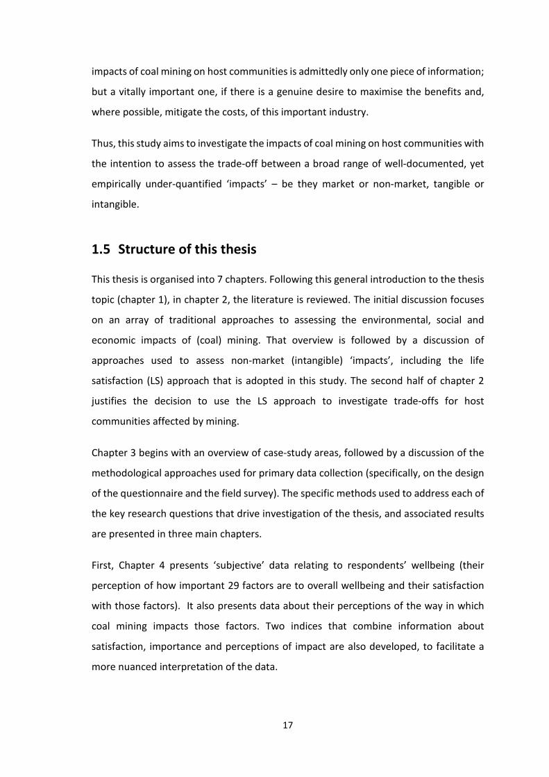
First, Chapter 4 presents ‘subjective’ data relating to respondents’ wellbeing (their

perception of how important 29 factors are to overall wellbeing and their satisfaction

with those factors). It also presents data about their perceptions of the way in which

coal mining impacts those factors. Two indices that combine information about

satisfaction, importance and perceptions of impact are also developed, to facilitate a

more nuanced interpretation of the data.

18

Second, Chapter 5 compares objective and subjective indicators of ‘wellbeing’ across the

5 types of case-study areas – the aim being to determine if the indicators convey similar

messages and can thus be used interchangeably. Regression analysis is then used to

further explore the relationship between objective and subjective indicators, controlling

for a range of other factors known to influence subjective assessments.

In the third main data chapter (6), the impacts of coal mining on various indicators of

subjective wellbeing (including satisfaction with different life domains and global life

satisfaction) are investigated – making it possible to consider ‘net impacts’ across

multiple factors within specific life domains and ‘net impacts’ across multiple domains.

This thesis closes with chapter 7, which summarises, synthesises and discusses key

findings, contributions, and the implications for public policy and future studies.

19

Thesis outline

20

2. CHAPTER 2 LITERATURE REVIEW

Chapter outline

2.1 Introduction

2.2 Approaches to assessing the impacts of coal mining

2.2.1 Traditional approaches to assessing the impacts of coal mining

2.2.2 Assessing the value of non-market goods

2.3 Human wellbeing

2.3.1 The definition and dimension of human wellbeing

2.3.2 Factors that contribute to human wellbeing

2.3.3 Wellbeing indicators used in the literature

2.4 Coal mining and human wellbeing

2.5 Literature examining human wellbeing in coal mining regions

2.5.1 Lack of holistic investigations into a range of wellbeing factors and the trade-off between benefits and costs

2.5.2 Lack of subjective wellbeing measurement

2.5.3 Lack of importance weighting

2.5.4 Lack of investigation into perception of local residents about impacts of mining

2.5.5 Lack of the empirical alignment between subjective and objective wellbeing measurement

2.5.6 Lack of comparison of different case-study areas characterized by different intensities of coal mining

2.6 Summary: research gaps and questions

21

2.1 Introduction

The previous chapter outlined the nature and scope of (coal) mining’s impacts, including

impacts on the biophysical, economic and social milieu of human beings. It concluded

that an essential challenge to governing bodies the world over is balancing the good

with the bad, and that such a balance should be considered at multiple geographical and

social scales and include both market and non-market values. While mining may deliver

net benefits for a country overall or for some sections of society at some locations, a

distributional analysis may reveal that at different social or geographical scales such net

benefits are not apparent and may indeed present as a net negative impact.

This chapter firstly summarizes the traditional methods used to investigate the impacts

of coal mining and identifies their limitations. This is followed by examining the

literature about non-market valuation techniques that could potentially address the

limitation of traditional methods to mining impact assessment (section 2.2). Literature

on the factors that contribute to wellbeing and indicators used to measure wellbeing is

reviewed in section 2.3. The connection between wellbeing and impacts of coal mining

is discussed in section 2.4. This chapter concludes with clearly identified research gaps;

associated research questions are proposed – which provide a focus for the

investigations reported on in subsequent chapters of the thesis.

2.2 Approaches to assessing the impacts of coal mining

Some of the benefits and costs of coal mining can be transacted through markets (e.g.

mining revenues and capital cost), while intangible impacts, such as those affecting most

environmental, cultural and social values, are not normally associated with goods or

services that are tradeable in the markets (Gillespie and Kragt, 2010). These ‘non-market’

values do not have prices attached to or associated with them. Thus, one of the

challenges of social decision making is to include all relevant values irrespective of

whether or not their ‘value’ is revealed via market mechanisms (e.g. through prices).

Non-market impacts, a core interest of this study, are most frequently assessed using

22

non-market valuation methods. There are several traditional and more recent,

innovative methods, which are examined below.

2.2.1 Traditional approaches to assessing the impacts of coal mining

Currently used common approaches to identifying and assess the significance of

mining’s impacts include environmental impact assessment (EIA), social impact

assessment (SIA) and economic impact assessments (EcIA). “Environmental assessment

requires that all impacts, ecological, economic, and sociological, be integrated.

Economic valuation [cost-benefit analysis (CBA)] permits this” (Hundloe et al., 1990, p.

55). CBA entails one to conduct non-market valuation studies to generate data for use

within the broader analysis (Ivanova et al., 2007; Gillespie and Kragt, 2010). The outputs

of these processes are then used by various government instrumentalities as one input

to help decide whether the benefits of a proposed project outweigh its negative impacts

to the extent that it makes the project desirable (Hundloe et al., 1990). These

approaches also identify those entities most affected by the negative impacts of the

project and the value of those impacts. This can then be used to design compensation

packages for stakeholders or to identify suitable ecological offsets.

2.2.1.1 EIA, SIA, and EcIA

EIA, is the most widely used assessment process. Formally, it is “the process of

identifying, predicting, evaluating and mitigating the biophysical, social, and other

relevant effects of development proposals prior to major decisions being taken and

commitments made” (IAIA, 1999). “Both EIA theory and statutory requirements ─ the

latter with some possible exceptions ─ emphasize that impacts are to be assessed in

relationship to ecological, social, and economic impacts” (Hundloe et al., 1990, p. 56).

EIAs often have embedded within them multiple-objective planning activities, including

separated sophisticated analyses of the effects of a project in terms of economic

efficiency, regional development, environmental and social impacts (Hundloe et al.,

1990).

23

The EIA process is backed by a legal framework in most countries and most countries

require an environmental impact assessment before giving permission to a mining

project (IAIA, 1999). However, in practice, EIA varies between countries. In many cases,

especially in developing countries, “implementation of EIA often falls considerably short

of international standards. They frequently suffer from insufficient consideration of

impacts, alternatives, and public participation. In the worst case, they are not conducted

at all” (Li, 2008, p. 1).

“The emergence of SIA during the 1990’s [is] a significant component of EIA and today

[it is] (sometimes) an independent activity” (Joyce and MacFarlane, 2001, p. 4). Social

impact assessment is a systematic process setting the scope for the assessment,

identifying and predicting the magnitude and significance of impacts, and devising

management plans to mitigate negative impacts and enhance positive social outcomes

(Rranks, 2012).

SIA involves the consideration of changes in a number of aspects: people’s way of life,

interaction with one another on a day-to-day basis; their culture (shared beliefs,

customs and values); their community (the cohesion, stability, character, services and

facilities); their environment (the quality of the physical environment, the adequacy of

lifelines and basic services, their safety, feeling of security and their access to resources)

(Burdge et al., 1995 and Cox and Miers, 1995, cited by Ivanova et al., 2007, p. 214).

SIA “focusing on those changes that are most important within a community rather than

on those that are easiest to measure or with which researchers are familiar” (Ivanova et

al., 2007, p. 214). Social Impact Assessment (SIA) is carried out by social scientists (Dutta

and Bandyopadhyay, 2010). It is a systematic process of identifying and mitigating

impacts on individuals or society, involved with public participation in consultation

with the individuals or society affected (Ivanova et al., 2007; Dutta and Bandyopadhyay,

2010).

Traditional economic impact assessment (EcIA) generates an estimate of the economic

consequences of a particular project, with an emphasis on changes in sales, income and

employment (Ivanova et al., 2007). The focus of EcIA is on understanding the likely order

of magnitude of impacts rather than the net benefits to society (Ivanova et al., 2007).

24

There are a range of tools that can be used for EcIA, such as input-output modelling, or

general equilibrium modelling (Jensen and West, 2002 and Rolfe et al., 2005a, cited by

Ivanova et al., 2007, p. 213).

An economic assessment often includes cost-benefit analysis (CBA) (Ivanova et al., 2007).

Distinct from the normal focus of an EcIA on the identification of income, spending and

employment impacts, CBA can provide some evaluation of the net impact of a project

(Ivanova et al., 2007). It incorporates ‘values’ that are not assessed by traditional impact

assessment, and thus allows one to consider trade-offs between all benefits and costs

irrespective of whether or not those benefits and costs are associated with the market

(Ivanova et al., 2007). It provides a structured way of aggregating monetised data about

benefits and costs – weighting them against each other according to specific rules (e.g.

including discount rates) (Atkinson and Mourato, 2006). However, it always encounters

difficulties in practice, as discussed in more detail below.

2.2.1.2 The comparison and application of traditional approaches to mining impact

assessment

Potential economic and social impacts are usually assessed through the EIA process

(Hundloe et al., 1990; Ivanova et al., 2007), which requires the application of SIA and

EcIA. Traditional EcIA focuses on the economic domain, and has the potential to identify

the net impact/trade-off of a (mining) project through CBA, but it may be too divorced

from the community of interests (Ivanova et al., 2007). In contrast, social impact

assessment can tap into different community groups, discover how they could be

affected in details and identify the important issues, but it fails to comprehensively

assess the trade-off between benefits and costs. The lack of integration of social and

economic impacts assessment techniques may limit the usefulness of their application

(Ivanova et al., 2005, 2007).

Cost-benefit analysis, in particular, can marry the environmental, social and economic

aspects of ‘impact’ and can provide a straightforward method for assessing the ‘net’

impact of a project (Hundloe et al., 1990; Atkinson and Mourato, 2006). There are a few

studies that have used CBA or approaches similar to CBA in mining contexts. For example,

Bai et al. (2011) used CBA to analyse the impacts of coal mining on local water eco-

25

services, economy and society, although it only focused on the negative impacts of coal

mining on water. Some analyses which are similar to CBA (in that they combining the

benefits and costs from coal mining) have been used in mining contexts: for example,

Hendryx and Ahern (2009) estimated the impacts of coal mining on public health (using

the value of statistical life lost) and the economic benefits of the coal mining industry;

None of these studies, however, address a wide range of biophysical and social impacts

identified throughout the world (and discussed in chapter 1); instead they generally

focus on just one or two non-market impacts.

Another relatively common framework, which attempts to consider damage to the

biophysical environment, is that of eco-compensation whereby the biophysical impacts

of mining are assessed and those stakeholders suffering a consequent economic loss are

compensated 4 . Existing studies on eco-compensation standards lack quantitative

assessments of the costs and benefits of numerous intangible impacts of coal mining on

the environment, economy and society, and there has been inadequate analysis of the

allocation of compensation among groups who compose the main stakeholders (Bai et

al., 2011).

Researchers have been exploring approaches to incorporate multiple intangible values

within these assessment frameworks with varying success (e.g. Noronha, 2001; Song,

2012). For example, Song (2012) proposed the concept of “General eco-economic

indices for mining exploration compensation” to calculate an eco-compensation

standard that incorporated economic losses resulting from damage to the environment.

Economic losses from air pollution and water pollution were calculated by comparing

the value of agricultural (and aquacultural) production before and after the mining (p.

139). This approach has much promise in agricultural regions, but may not be useful in

other regions ─ particularly if one does not have data on agricultural production ‘before’

and ‘after’ coal mines emerged. Also, the ‘value’ of some environmental impacts, such

as those associated with noise and visual amenity are not captured by this type of

4 “Ecological compensation in a coal mining region can be classified as either broad or narrow. Broad ecological compensation is carried out mainly through land requisition, relocation, and ecological reconstruction, as well as by supporting resource-based cities [regions] to achieve sustainable development. Narrow ecological compensation only includes land reclamation and ecological reconstruction” (Bai et al., 2011, p. 144). Ecological compensation here refers to the broad definition.

26

analysis which focuses only on agricultural production (goods and services that are more

closely associated with the market) – the ‘tangible’ impacts of degradation. Additionally,

this framework has, thus far, been unable to incorporate the potential impact of rising

inequality or losses in social capital that may be associated with mining, nor has it been

able to offer a strong and straightforward estimate of the net impact of mining on the

host communities to inform public policies.

In theory, a comprehensive CBA includes estimates of all benefits and all costs

associated with the project/program being evaluated, using a common measuring rod

(Hundloe et al.,1990) – traditionally, a monetary one. Likewise, a comprehensive eco-

compensation assessment should estimate the financial dollar equivalent of all the

damage (costs) associated with a mine. The current studies cited above which use CBA

or approaches similar to CBA, as well as the eco-compensation, all attempt to assess

impacts that are not directly traded in the market but are, nonetheless, indirectly

associated with the market (e.g. damage to agricultural land implies loss of agricultural

production). The values of these non-market impacts can thus be inferred through the

market, using either market or revealed market approaches, which will be discussed in

detail in the following section.

But mining impacts many things which have little or no link to marketed goods and

services, thus requiring CBA and eco-ceompensation researchers to undertake other

non-market valuation exercises (that rely on hypothetical markets), for use in the wider

analysis. The more ‘intangible’, and more loosely connected an impact is to the market,

the more difficult it is to adequately measure. The quality of the broader CBA (or similar)

studies will thus depend, at least in part, on the quality of the non-market valuation

study that estimates the ‘value’ of these various non-market impacts. Measuring these

impacts (particularly the intangible impacts) using a monetary measuring rod is not a

trivial task, which explains why the current literature cited above usually assess limited

number of non-market impacts.

While highly useful as a decision-making tool, CBA thus suffers from multiple limitations,

which derive from behavioural and scientific uncertainty and the difficulty of bringing all

relevant variables to a common monetary base to allow their addition when calculating

27

net benefit. In practice, it is often too difficult to generate monetary estimates of the

‘value’ of all non-market impacts, so many are often omitted from the analysis. These

problems have limited the theoretically wide scope of both CBA (Hundloe et al., 1990)

and eco-compensation. This might also help explain why CBA is not widely used to assess

the impact of mining activity (Ivanova et al., 2007) and why many of the known impacts

of mining are excluded from the assessments of eco-compensation.

2.2.2 Assessing the value of non-market goods

As explored above, many of the limitations of traditional methods used to assess the

impacts of mining arise from the challenges of estimating the value of numerous

intangible and difficult-to-monetise impacts. Much research effort has been invested in

developing techniques to allow reliable monetary expression of the value of non-market

goods. While considerable progress has been made, significant challenges remain and

to date the validity and reliability of monetary evaluations of non-market goods remains

contentious. The following sections expand on some of the more common approaches

to non-market valuation designed to overcome the difficulties inherent in common

impact assessment practice.

2.2.2.1 Traditional approaches which generate monetary estimates of the ‘value’ of

non-market goods and their applications in mining contexts

There is a large body of literature that looks at ways of assessing the non-market goods

in monetary terms, so that they can be compared with other (monetary) values on a

somewhat equal footing. Termed “Economic valuation methods”, these approaches can

estimate the effect of changes in either the quantity or quality of non-market goods on

utility (Dolan and White, 2007). Broadly, valuation methods fall into one of three main

types: market-based approaches (MB), revealed preference approaches (RP) and stated

preference (SP) approaches. The life satisfaction (LS) approach (discussed in the

following sub-section) is an emerging, non-traditional valuation approach that offers

much promise (Dolan and Metcalfe, 2007).

MB approaches essentially rely on observable market prices, costs, expenditures or

revenues. For example, they assess the ‘value’ of changes in agricultural production or

28

the cost of repairing damaged structures (Loomis et al., 2003; Morrison, 2009; Li et al.,

2011). These approaches can only be used to assess impacts that are directly related to

the market (if impacts are not directly related to the market, one cannot obtain price,

cost or expenditure/revenue data). Another limitation of MB approaches is that “they

only provide a lower bound on community values as the community may be willing to

pay more than the replacement cost to prevent damage” (Morrison, 2009, p. 11).

RP approaches include techniques such as hedonic pricing and the travel cost method

and do not require one to be able to directly ‘observe’ market prices. Instead, these

approaches use “complementarity or substitute relationships between environmental

goods and market goods to infer the value attributed to environmental conditions from

observed behaviour with respect to market goods” (Welsch, 2006, p. 802).

Rather than using actual or ‘related’ markets to infer values, SP approaches use

hypothetical approaches. Formally, individuals are directly asked to value

environmental goods, using specially constructed questionnaires to capture an

individual’s willingness to bear a financial impost in order to achieve some potential

(non-financial) environmental improvement, or avoid some potential environmental

harm (Bennett and Blamey, 2001). Examples are the contingent valuation (CV) method

and the choice modelling or choice experiment method (de Bekker‐Grob et al., 2012).

The contingent valuation method focuses on valuing a non-market good as a whole,

while the choice modelling/experiment method focuses on valuing specific attributes of

a non-market good (Welsch, 2006; Fujiwara and Campbell, 2011). Choice modelling,

grounded in random utility theory, assumes that the benefit of an attribute (A) can be

measured in terms of the frequency with which a person chooses A over a competing

attribute (B) (Centre for International Economics, 2001).

Both RP and SP approaches have significant disadvantages. RP methods are based on

“stringent assumptions concerning the rationality of agents and the functioning of

markets” (Welsch, 2006, p. 802). SP surveys use hypothetical scenarios from the

respondents, which may entail unreliable results and strategic behaviour (Welsch, 2006).

Both RP and SP can only capture those impacts that individuals are actually aware of.

The values that individuals are not aware of cannot be captured, although they exist

29

(Welsch, 2006). Choice modelling is considered superior to conventional SP methods, as

the instrument used to gain the information of ‘willingness to pay’ forces respondents

to consider multiple trade-offs between attributes. However, the attributes involved are

limited to 6 or 7, as respondents have difficulty processing more than this number

(Centre for International Economics, 2001).

As mentioned in the previous section, most previous studies that have estimated the

non-market impacts (but directly associated to market) of coal mining or mining using

MB approaches (e.g. Noronha, 2001; Hendryx and Ahern, 2009; Epstein et al., 2011; Li

et al., 2011; Song, 2012). Studies using RP and SP to assess those impacts not directly

associated with the market are relatively few, but they do exist.

Using hedonic pricing to assess the values of the environmental impacts of coal mining,

Trigg and Dubourg (1993) found that the environmental costs of coal mining in the UK

significantly reduced its economic viability. Ivanova et al. (2007) were one of the first to

use choice modelling within an integrated assessment of the impacts of coal mining in

the Bowen Basin, Australia. They used results from the choice modelling study to help

assess the trade-off between social and economic costs and benefits, arguing that the

results should be put in the context of wider issues that arose from the stakeholder

analysis. The study of Gillespie and Kragt (2010), a more recent one, used discrete choice

experiments to value the non-market environmental, cultural and social impacts of

underground coal mining and incorporated the derived values into the frame of CBA.

The shortcomings of existing studies using MB, RP and SP are derived from the inherent

disadvantage of the approaches they adopted. One of the limitations of studies using

MB has been discussed in detail in the last section, for example, they can only assess

impacts that are directly related to the market. But another, more fundamental

shortcoming of these studies is that they only deal with a limited number of impacts

associated with coal mining. This is not a reflection on the quality of the analysis

undertaken by researcher, but rather a reflection of the great empirical difficulty of

undertaking these non-market valuation studies – they involve significant amounts of

time, data, and sophisticated analyses to generate reliable estimates. Trigg and Dubourg

(1993), for example, only consider environmental impacts; Gillespie and Kragt (2010)

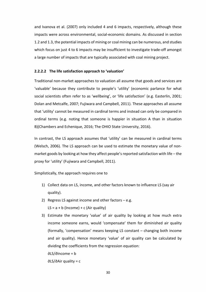
30

and Ivanova et al. (2007) only included 4 and 6 impacts, respectively, although these

impacts were across environmental, social-economic domains. As discussed in section

1.2 and 1.3, the potential impacts of mining or coal mining can be numerous, and studies

which focus on just 4 to 6 impacts may be insufficient to investigate trade-off amongst

a large number of impacts that are typically associated with coal mining project.

2.2.2.2 The life satisfaction approach to ‘valuation’

Traditional non-market approaches to valuation all assume that goods and services are

‘valuable’ because they contribute to people’s ‘utility’ (economic parlance for what

social scientists often refer to as ‘wellbeing’, or ‘life satisfaction’ (e.g. Easterlin, 2001;

Dolan and Metcalfe, 2007; Fujiwara and Campbell, 2011). These approaches all assume

that ‘utility’ cannot be measured in cardinal terms and instead can only be compared in

ordinal terms (e.g. noting that someone is happier in situation A than in situation

B)(Chambers and Echenique, 2016; The OHIO State University, 2016).

In contrast, the LS approach assumes that ‘utility’ can be measured in cardinal terms

(Welsch, 2006). The LS approach can be used to estimate the monetary value of non-

market goods by looking at how they affect people’s reported satisfaction with life ─ the

proxy for ‘utility’ (Fujiwara and Campbell, 2011).

Simplistically, the approach requires one to

1) Collect data on LS, income, and other factors known to influence LS (say air

quality).

2) Regress LS against income and other factors ─ e.g.

LS = a + b (Income) + c (Air quality)

3) Estimate the monetary ‘value’ of air quality by looking at how much extra

income someone earns, would ‘compensate’ them for diminished air quality

(formally, ‘compensation’ means keeping LS constant ─ changing both income

and air quality). Hence monetary ‘value’ of air quality can be calculated by

dividing the coefficients from the regression equation:

∂LS/∂Income = b

∂LS/∂Air quality = c

31

∂Air quality/∂Income = c/b

In other words, by comparing the marginal utility/disutility of non-market goods, with

that of income, the trade-off between income and non-market goods can be determined,

providing a monetary value of the non-market factor/good of interest.

This approach has several advantages over traditional non-market valuation approaches.

Firstly, in contrast to RP and SP approaches, the LS approach does not presume rational

agents and perfect markets (Frey et al., 2004; Welsch, 2006). Secondly, this technique

does not rely on asking people how they value “public goods or bads/negative and

positive externalities” (Frey et al., 2004, p. 5), nor does the LS approach require an

individual to fully understand cause and effect relationships. Instead, individuals are

asked in surveys how satisfied they are with life, and econometric analysis is used to

identify if and how their answers change with different amounts (or qualities) of non-

market goods. For these reasons the life satisfaction approach is cognitively less

demanding on respondents than contingent valuation and choice modelling and does

not evoke response bias (Welsch, 2006). Thirdly, there is no reason to expect strategic

behaviour, since the survey questions do not relate to the target non-market goods in

any way.

However, it is uncertain whether LS data is a good measure of utility (Ambrey and

Fleming, 2011). Three major difficulties identified and discussed by (Fujiwara and

Campbell, 2011) include:

(1) Remembering past experiences. People who remember and emphasize past

experience/utility might lead to biased judgement of current life satisfaction;

(2) Context effects. People may take their current mood as a good indicator of their

wellbeing in life in general (Schwarz and Strack, 1999);

(3) Reporting LS. When reporting LS in a face-to-face interview, individuals may adjust

their life satisfaction scores in order to give more socially desirable responses. For

example, reported life satisfaction level is higher in face-to-face surveys than in postal.

32

In spite of the limitations above, the LS approach is an effective way to value non-market

goods. The body of literature that uses this approach to consider the ‘value’ of a range

of non-market goods and services is growing rapidly and includes studies of: airport

noise (Van Praag and Baarsma, 2005), air pollution (Welsch, 2006; Luechinger, 2009;

MacKerron and Mourato, 2009), inequality (Blau and Blau, 1982), terrorism (Frey et al.,

2009), corruption (Welsch, 2008) and disasters (Luechinger and Raschky, 2009). In these

and other studies, reported life satisfaction has been used as an empirically adequate

and valid approximation for individual utility.

However, to the best of my knowledge, the LS approach has not been used to contribute

to the assessment of the impacts of mining industries or projects, and the challenge to

fully incorporate impacts on non-market environmental and social aspects remains.

The following section will discuss the emerging literature on life satisfaction or wellbeing,

as well as the feasibility of using the life satisfaction (wellbeing) approach to assess the

multiple impacts of mining and to explore the trade-off between the benefits and costs

of mining industries or projects.

2.3 Human wellbeing

Terms related to “wellbeing” in the literature are “life satisfaction”, “subjective

wellbeing”, “happiness”, and “quality of life (QOL)”. These terms are often used

interchangeably: see Easterlin (2003a), Rehdanz and Maddison (2005), Costanza et al.,

(2007), Johns and Ormerod (2007) and Dolan and Metcalfe (2007) as examples. Life

satisfaction or happiness is conceived as a measure of “the degree to which an individual

judges the overall quality of his or her life-as-a-whole favourably or unfavourably”

(Ehrhardt et al., 2000, p. 181). This is sometimes termed global life satisfaction (GLS). In

this study, life satisfaction or GLS is thought to be one of the dimensions of subjective

wellbeing, and subjective wellbeing is one of the measurements of wellbeing, detailed

in 2.3.1.2. In contrast, the phrase of “quality of life” is closer to that of “wellbeing”, as

they both refer to objective and subjective measurements of numerous factors; these

two terms are thus sometimes used interchangeably (e.g. Van Praag and Baarsma, 2005;

Costanza et al., 2007). This will be discussed further in the following section.

33

2.3.1 The definition and dimension of human wellbeing

2.3.1.1 Definitions of human wellbeing

The term ‘wellbeing’ or “human wellbeing” is used in various disciplines, such as

economics, psychology, and sociology. Because these different disciplines use differing

research instruments, have different standpoints, ask different types of questions, and

are based upon different theoretical views and ontological presuppositions (Gasper,

2010), the definition, measurement and determinants of wellbeing are not used with

great consistency or precision (Kahn and Juster, 2002; Dodge et al., 2012; Rablen, 2012).

As such, it may be best to think of the term ‘wellbeing’ as having different roles and

occasions of relevance, and then select a particular definition or build a particular

synthesis to serve a particular research purpose (Gasper, 2010).

Despite the complexity and difficulty of pinning down a single definition of wellbeing, it

is widely accepted by researchers that wellbeing contains subjective and objective

dimensions (Dale, 1980; Muldoon et al., 1998; Veenhoven, 2002; Gasper, 2004, 2005,

2010; Oswald and Wu, 2010). A categorization of conceptions of wellbeing by Parfit

(1984) has become widely used in philosophical ethics (Muldoon et al., 1998; Gasper,

2004). They are as follows: 1) In hedonism, wellbeing is seen as the pleasure – a mental

statement; 2) In desire theories: wellbeing is seen as preference/desire fulfilment; and

3) In objective list theories, it is understood as the satisfaction with the substantive list

of elements that make a life well lived. Evidently, any single one of these understandings

of the concept is incomplete (Gasper, 2004); a comprehensive conception or

measurement of wellbeing should include both objective and subjective dimension.

2.3.1.2 Objective wellbeing and subjective wellbeing

According to Gasper (2010), there is far more than a binary contrast between ‘subjective

wellbeing’ (SWB) and ‘objective wellbeing’ (OWB). Both objective and subjective

wellbeing can refer to subjective states or to a person’s condition and circumstances,

can be undertaken using private values or values endorsed through a public procedure,

and can be self-reported or be externally observed (Gasper, 2010). There are many

relevant interpretations of both ‘objective’ and ‘subjective’ wellbeing, and the two

34

concepts overlap, but one of the most popular distinctions between the two – preferred

by Gasper (2010) and other researchers, relates to the fact that SWB focuses on

subjective states, while OWB focuses on a person’s conditions and circumstances

(Gasper, 2010).

The well-accepted and most often cited definition and application of OWB and SWB is

as follows. Objective wellbeing (OWB) refers to an “objective view of a person’s

wellbeing given their objective circumstances” (Rablen, 2012, p. 299). It is a measure of

‘hard’ facts (Veenhoven, 2002) and observable variables, that we generally believe are

important for a good life (Argyle, 2001). Objective indicators, generally defined as counts

of various types of phenomena (e.g. life expectancy, levels of income and education,

residential, densities and unemployment figures, and pollution levels) are most often

regarded as quantitative facts and are often selected from census data and other

accessible and verifiable official registers (Dale, 1980). OWB can be expressed as a set

of indicators (e.g. economic wellbeing, social welfare and the status of the bio-physical

environment) or a single composite index (Lepper and McAndrew, 2008).

SWB refers to ‘soft’ matters (Veenhoven, 2002), and is measured by general mental-

state accounts of an individual’s personal assessment of his/her life (Dolan and White,

2007) or subjective responses of likes and dislikes (Dolan and White, 2007; Lepper and

McAndrew, 2008; Rablen, 2012). According to Diener (2000), subjective wellbeing

consists of four components: global life satisfaction, satisfaction with important life

domains, positive effects of experiencing pleasant emotions and moods, or, conversely,

negative effects of experiencing unpleasant emotions and moods. Global life satisfaction

and satisfaction with discrete life domains are the two basic approaches to the definition

and measurement of subjective life quality (Cummins, 1996). Global life satisfaction is

the most commonly used of measures of life evaluation, and satisfaction with important

domains, is proved to be strongly related to overall life evaluations (OECD, 2013).

Examples of SWB indicators are life satisfaction (LS), and the Happiness Index. These

indicators are sourced from empirical surveys, or in some countries from various

databases such as in the World Database of Happiness (EHERO, 2014), and the Personal

Wellbeing Index (The International Wellbeing Group, 2013).

35

2.3.1.3 The application of OWB and SWB and the relationship between OWB and

SWB

Governments tend to pursue the more easily obtained objective indicators of wellbeing,

while paying less consideration to examining and improving subjective wellbeing (Diener

and Suh, 1997; Abdallah et al., 2011; Rablen, 2012). For instance, the objective approach

is currently dominant in the Scandinavian countries, in particular in the Swedish ‘level

of living’ studies (Veenhoven, 2002). The UK National Indicators that are used to

evaluate local government consist primarily of objective indicators such as crime,

mortality, and employment rates (Rablen, 2012).

The reluctance among policymakers to reduce reliance on OWB is probably because it

can be measured by tangible indicators that are relatively easy to collect and understand,

and are relatively easily connected to government policies and budgets. But OWB may

be heavily influenced by the values of those who construct indicators to measure it; such

measures may thus not reflect public preference (Rablen, 2012) and/or may do little to

inform makers of public policy (Veenhoven, 2002). Moreover, objective indicators fall

short in measuring some intangible factors, such as trust and perceived street safety

(Veenhoven, 2002), which partly explain why these values (or many other intangible

values) are not measured by the official department. In contrast, SWB requires data

about intangible concepts, such as people’s thoughts and emotions (Rablen, 2012).

Concerns that have been raised about indicators of SWB, focus on the fact that they may

lack direct and obvious connections to government policy and budgets (Rablen, 2012).

That said, there is much support for subjective indicators ─ the OECD (2013), for example,

argues that the drivers of social policy should not be limited to information about

material matters, but should also be informed by peoples’ judgment of their lived

experience, requiring the recruitment of subjective indicators.

Measures of SWB are now at the forefront of some academic analyses (Chen and Lin,

2014), and “are generally found to have a high scientific standard in terms of internal

consistency, reliability and validity and a high degree of stability over time” (Welsch,

2006, p. 803). The International Wellbeing Index (IWI) has been used to measure

subjective wellbeing in many western countries (The International Wellbeing Group,

36

2013) and developing countries, such as China (Knight et al., 2009; Davey and Rato, 2012;

Monk-Turner and Turner, 2012).

Empirical studies that have explored the relationship between objective measurements

and subjective measurements tend to be contradictory. For example, Schneider (1975)

examined ‘quality of life’ rankings of US cities based on objective wellbeing indicators

and subjective indicators of quality of life, and concluded that the level of wellbeing,

measured by objective indicators, did not predict the subjective life quality experienced

by individuals living in those cities. In contrast, Oswald and Wu (2010) found that the

ranking of quality of life in each US state was consistent between subjective and

objective approach. Emmons and Diener (1985) found that objective conditions were

only predictive of satisfaction in a few domains. Differences between these studies will

be further discussed later in this chapter.

Given the unconfirmed relationship between OWB and SWB, and given that both

concepts have strengths and weaknesses, they are complementary and are both needed

to obtain a comprehensive baseline picture of wellbeing in any jurisdiction or

community against which development outcomes for society may be gauged (Dale, 1980;

Diener and Suh, 1997; Veenhoven, 2002).

2.3.2 Factors that contribute to human wellbeing

The multiple impacts of coal mining were detailed in chapter 1. This section reviews the

literature that addresses the following two questions. “Do the factors that coal mining

have impacts on contribute to wellbeing or life satisfaction? And “What is the

relationship between coal mining and human wellbeing or life satisfaction?”

The expanded full world model of the ecological economic system elaborated by

Costanza et al. (1997) (see Figure 2.1) describes the interaction between wellbeing and

four basic types of capitals.

37

Figure 2.1 Full World Model of the Ecological Economic System

Source: From ‘An Introduction to Ecological Economics’ (Costanza et al., 1997, p. 275).

At the core of this model is the set of four basic types of capitals: natural, human, social,

and built capital, and these four kinds of capital under the strict interpretation of

sustainability are not seen as interchangeable (Costanza et al., 1997). Both economic

goods and services and ecological services and amenities are produced and contribute

in different ways to satisfying basic human needs and creating both individual and

community wellbeing. The economic process generates waste and in doing so exerts a

negative effect on wellbeing, as well as on capitals and ecological services (Costanza et

al., 1997).

2.3.2.1 Natural capital and human wellbeing

Costanza et al. (2007) define natural capital as the “renewable and non-renewable

goods and services provided by the ecosystems” (p. 271). Human beings depend on

these systems for a variety of goods and services. As shown in Costanza’s diagram

(Figure 2.1), natural capital can contribute to wellbeing in three ways: directly (by, for

example, providing an aesthetic experience); indirectly through the provision of

38

‘ecosystem services’ 5 ; and indirectly, when combined with other capitals in the

economic production ‘process’ to generate other goods and services. A large body of

literature by communities of economists, environmental scientists and psychologists has

studied and firmly established that a good environmental quality significantly

contributes to human wellbeing, while bad environmental quality reduces wellbeing (e.g.

Welsch, 2002; Van Praag and Baarsma, 2005; Luechinger, 2009; MacKerron and

Mourato, 2009; Ferreira and Moro, 2010; Menz and Welsch, 2010; Levinson, 2012;

Cuñado and de Gracia, 2013; Guardiola et al., 2013).

2.3.2.2 Human capital and human wellbeing

Human capital is often conceptualised as a measure of people’s ability to produce goods

and services that have ‘economic value’; it thus often refers to physical labour and to

‘know-how’ (Ekins, 1992; Earth Inc., 2007). Education is often chosen as a proxy measure

of human capital.

Most previous studies have found that the accumulation of human capital contributes

to wellbeing: education is frequently found to be positively correlated with reported

levels of satisfaction (e.g. Di Tella et al., 2003; Ferrer-i-Carbonell & Gowdy, 2007; Welsch,

2007b; Brereton et al., 2008; Smyth et al., 2011). Diener et al. (1999) argue that

education may also indirectly affect subjective wellbeing through other variables. Those

with a higher education also generally have a higher income, are in better physical health

and have higher participation rates in social activities (compared to those with less

education) all of which are essential to wellbeing (Healy and Côté, 2001; Clark and

Oswald, 2002; Frey and Stutzer, 2002b; Di Tella et al., 2003).

Some studies have, however, found a negative association between education and life

satisfaction (e.g. Clark and Oswald 1996; Arifwidodo and Perera, 2011). One plausible

explanation for this negative relationship is that education raises expectations;

therefore, a comparison effect happens, where more highly educated people have a

5 The Millennium Ecosystem Assessment (MEA), was one of the first, widely cited, frameworks for describing the important role that ecosystem services play for human wellbeing. In particular, this framework demonstrated how ecosystems services contribute to constituents of wellbeing, including security, basic material for a good life and health (Corvalan et al., 2005).

39

higher expectation for Quality Of Life (QOL), which lowers the actual condition of QOL

(Clark and Oswald, 1996; Arifwidodo and Perera, 2011).

2.3.2.3 Social capital and human wellbeing

A substantial amount of literature shows evidence of a strong correlation between social

capital and life satisfaction (e.g. Helliwell, 2003; Engelbrecht, 2009; Bartolini and

Sarracino, 2011). Those who have frequent contact with family, friends and neighbours

have higher reported levels of wellbeing than those with less contact (Helliwell and

Putnam, 2004).

That said, it is not always easy to determine how to define and ‘measure’ social capital.

Some researchers have argued that a measure of generalized trust is part of what is

meant by the phrase ‘social capital’, while others have preferred to treat interpersonal

trust as something that is generated and supported by other types of social capital

(Helliwell, 2001), such as laws, political factors, economic factors, and crime rates within

society (Vemuri and Costanza, 2006).

2.3.2.4 Manufactured capital and human wellbeing

Manufactured or built capital comprises goods “such as tools, equipment and buildings”

(Costanza et al., 2007, p. 271), used for the production of goods and services (Helliwell

and Putnam, 2004). As we all know, urban places supply more manufactured goods than

rural places. Differences in the spatial organization and capital goods between urban

and rural areas thus result in different socioeconomic outcomes that affect human

wellbeing (Cutler et al., 1997; Vemuri and Costanza, 2006). There is a growing conviction

among urban and regional policy makers that the character of the built environment is

one of the factors influencing quality of life (QOL) (Arifwidodo and Perera, 2011).

A study exploring the relationship between QOL and the urban spatial pattern in

Bandung city, Indonesia reveals a positive and significant relationship between self-

reported wellbeing and the availability of urban facilities (Arifwidodo and Perera, 2011).

Brereton et al. (2008) use the proximity to various built capital, such as landfill, rail

station, airport, seaports and national/secondary roads to analyse Irish life satisfaction

40

data. They conclude that: proximity to landfill has a negative effect on wellbeing, while

proximity to the coast has a largely positive effect, diminishing with distance. The impact

of proximity or easy access to major transport routes has different effects depending on

the type of, and distance to, the amenity in question.

Vemuri and Costanza (2006) used the UN’s Human Development Index (HDI) (1995)

obtained from the United Nations Human Development Report (1998), as a composite

of human and built capital. The HDI is a measure of human development, which

comprises “a longevity index, an education index, and a standard of living index”

(Vemuri and Costanza, 2006, p. 123). The reason to represent the human and built

capital variables together was due to the high correlation between human capital

variables and all the possible built capital variables (Vemuri and Costanza, 2006).

2.3.2.5 Institutional capital and human wellbeing

Although institutional capital is not included in the “full world” model, the literature

demonstrates that the quality of institutions affects subjective wellbeing (e.g. Frey and

Stutzer, 2000; Rehdanz and Maddison, 2005; Engelbrecht, 2009; Frey and Stutzer, 2010).

Several proxies to measure institutional capital have been used, including levels of

democracy, civil liberty, political rights, economic freedom, good governance and

corruption in those literature. In particular, the efficiency and trustworthiness of the

design and delivery of government were found of primary importance for poor countries,

while more value appeared to be attached to building and maintaining the institutions

of electoral democracy in developed countries (Helliwell and Huang, 2008).

2.3.2.6 Other factors that affect human wellbeing

(1) Income, income inequity and employment

Income is cited in most studies of wellbeing (e.g. Adamowicz et al., 1998; Diener, 2000;

Diener and Oishi, 2000; McBride, 2001; Ferrer-i-Carbonell, 2005; Kahneman and Deaton,

2010), and the relationship between income and subjective wellbeing is the major focus

of many of these studies.

41

At the macro level (e.g. GDP per capita), cross-country studies show that, in

industrialized/developed countries the rise of real national income bring little or only a

small amount of extra happiness over time (Easterlin, 1974; Oswald, 1997). However,

the effect of income on wellbeing is significantly stronger in developing countries and/or

in regions with relatively high unemployment rates (Stanca, 2008). In general, the main

factors that improve quality of life in poor countries seems to be income, but once a

certain level of development is attained, the main attributes that influence wellbeing

are other factors, such as friends and good family life (Costanza et al., 2007; Arifwidodo

and Perera, 2011). More will be discussed of this complicated relationship between

economic growth and wellbeing in section 2.4.

At the micro level (household or individual income), the effects of income on human

wellbeing differ across case-study areas. For example, Frey and Stutzer (1999, 2000)

found that improvements in financial situation hardly raise happiness in Sweden, while

other studies found that higher household or individual income was statistically

correlated with higher levels of life satisfaction or quality of life, in developed countries

(Van Praag and Baarsma, 2005; Welsch, 2006, 2008; Luechinger, 2009; MacKerron and

Mourato, 2009) and developing countries (Arifwidodo and Perera, 2011).

Income inequality also negatively affects human wellbeing (e.g. Daly, 1987; Diener et al.,

1999; Easterlin, 1995, 2003; Layard 2003; Stutzer and Frey, 2010). Increases in income

do not always contribute to increases in subjective wellbeing in OECD countries, but the

effect of relative income on subjective wellbeing in both OECD and developing countries

is obvious, and this effect is larger in the developing world (Helliwell, 2003). Once basic

needs are met, it seems that simple increases in income do less to raise life satisfaction.

What starts to matter more, apparently, is to earn more than others (Helliwell, 2003) –

thus the effect of income on life satisfaction appears to change as the average income

of a country evolves (Costanza et al., 2007; Arifwidodo and Perera, 2011).

At a micro-economic level, employment status, which is closely associated with income,

also influences human wellbeing (Frey and Stutzer, 1999b; Ballas and Dorling, 2007;

Brereton et al., 2008). At a macro-economic level, the national inflation rate and

unemployment have also been found to be negatively associated with national

42

measures of wellbeing (Di Tella et al., 2001; Engelbrecht, 2009). Unemployment is

invariably associated with lower levels of wellbeig (Oswald, 1997), and the effect of

unemployment on wellbeing is significantly stronger in countries with higher GDP per

capita and higher unemployment rate (Stanca, 2008).

(2) Sociodemographic factors

Linked to the discussion of social capital, being in a stable marriage and good quality of

interpersonal relations also has a positive and statistically significant relationship with

wellbeing; those being separated or divorced generally report low levels of wellbeing

(Ferrer‐i‐Carbonell and Frijters, 2004; Ferrer-i-Carbonell and Gowdy, 2007; Brereton

et al., 2008; Arifwidodo and Perera, 2011). Clark and Oswald (2002) report that getting

married could increase overall life satisfaction (happiness) by the same amount as an

extra 70,000 $US of income per annum; widowhood would reduce happiness by an

amount equivalent to a reduction in income of 170, 000 $US per annum.

Age is one of the most cited sociodemographic determinants of human wellbeing. Age

reflects the life cycle pattern in human wellbeing and shows a consistent U-shaped

relationship with life satisfaction falling until mid-life, then rising with age (e.g. Di Tella

et al., 2003; Brereton et al., 2008).

Subjective wellbeing has also been shown to be affected by the following

sociodemographic variables: (1) family size (Frijters and Van Praag, 1998; Frey and

Stutzer, 2000; Moro et al., 2008; Stutzer and Frey, 2008) (2) house type/tenure

(Brereton et al., 2008; Moro et al., 2008); (3) gender (Frey and Stutzer, 2000; Brereton

et al., 2008; Moro et al., 2008; Arifwidodo and Perera, 2011).

(3) Genetic factors

It is widely acknowledged that both happiness and depression can be hereditary (e.g.

Sullivan et al., 2000; Lyubomirsky et al., 2005; Zidanšek, 2007). Research on identical

twins suggests that genetics explains around 50% of all observed differences in reported

‘happiness’ or life satisfaction level (Lyubomirsky et al., 2005; Zidanšek, 2007). More

specifically: genetic factors have been estimated to account for between 39% and 58%

43

(Tellegen et al., 1988) or between 40% and 55% (Diener et al., 1999) of happiness in

adults; and between 35% and 57% of happiness in children (Braungart et al., 1992) As It

is extremely difficult to obtain genetic information for standard LS studies, researchers

must content themselves with exploring the influence of other factors, knowing that

their final models might be unlikely to account for more than 50 % of all variation.

2.3.3 Wellbeing indicators used in the literature

The previous section discussed the four types of capital that support human wellbeing,

as well as some other factors that were found to influence wellbeing. Evidently, the

number of different factors that affect wellbeing are enormous and diverse (Cummins,

1996). However, these factors are frequently related (e.g. income and education), so

variables (or indicators) that are used in empirical studies to capture the influence of

factors on wellbeing often share a great deal of their variances. Cummins (1996)

demonstrated that 68% of 173 different variables from the literature could be grouped

into seven life “domains”, including material wellbeing, health, productivity, intimacy,

safety, community emotional wellbeing and spirituality.

There are several well-documented studies of wellbeing which consider numerous life

domains including (but not limited to) the wellbeing indicators of OECD (OECD, 2011)

and the International Wellbeing Index (The International Wellbeing Group, 2013). These

examples (below) highlight the fact that there is no commonly agreed set of ‘domains’

about which researchers and organisations who are interested in wellbeing regularly

collect data.

44

Figure 2.2 Framework for OECD wellbeing indicators

Source: From ‘Compendium of OECD well-being indicators’ (OECD, 2011, p. 5).

In the OECD’s framework of wellbeing indicators (Figure 2.2), subjective wellbeing only

refers to how people evaluate their life as a whole, without measuring the satisfaction

with different wellbeing factors. Other factors, such as health status, work and life

balance etc., apart from global life satisfaction, are all measured by objective wellbeing

indicators.

The International Wellbeing Index (IWI), including Personal Wellbeing Index (PWI) and

National Wellbeing Index (NWI), is the measurement of subjective wellbeing that has

been applied to many countries (Knight et al., 2009; Davey and Rato, 2012; Monk-Turner

and Turner, 2012; The International Wellbeing Group, 2013). The NWI measures

satisfaction with various conditions in a country, region, or city via six domains: business,

economic, social situation, environment, government, security and social conditions,

while the PWI measures individual satisfaction with domains relating to personal health,

achievement in life, personal relationships, personal safety, community connectedness

and future security (The International Wellbeing Group, 2013).

45

2.4 Coal mining and human wellbeing

Human wellbeing is affected by various environmental, economic, social and

psychological variables. As discussed in section 1.2 and 1.3, coal mining has multiple

impacts on various life domains, which are essential to human wellbeing. If something

(say coal mining) has multiple impacts on the environment, economy, society and

individual, then it is difficult to determine, a priori what the total effect on wellbeing will

be.

As discussed in chapter 1, although coal mining has various impacts on environmental,

economic, social domains, it is essential for economic growth, and may help increase

incomes and alleviate poverty, especially in underdeveloped countries or regions.

However, caution should be exerted if economic growth is seen as a final goal of human

development, because economic growth does not necessarily indicate a higher level of

subjective wellbeing. This has been highlighted by numerous researchers – a recent

example being Easterlin and Sawangfa (2009) who examined the relation between long-

term economic growth and growth rate of subjective wellbeing in 13 developing

countries with a time span of 16 years. They concluded that economic growth does not

necessarily increase subjective wellbeing. Daly and Farley (2010) also argued that

subjective wellbeing declines after a certain level of economic growth is reached, which

is identifies as uneconomic growth (see Figure 2.3).

46

Figure 2.3 Limits to the economic growth

Source: From ‘Three limits to growth’ (Daly, 2014) 6, accessed on 25th August 2015.

Here utility, substituted with life satisfaction (LS) in the LS studies, refers to the overall

satisfaction that a person gains from the consumption of a good or service (in the

diagram, the good is presumed to be ‘income’ ─ or, from a macroeconomic perspective,

GDP). Marginal utility is the additional benefit or satisfaction derived from obtaining an

additional unit of that good or service (i.e. a little more GDP). The law of diminishing

marginal utility states that the more one has of something, the less satisfaction an

additional unit provides. Contrarily, marginal disutility is the additional cost of producing

one more unit. In this case, it might be the amount of leisure time, or natural resources

are given up to produce more GDP. The law of increasing in marginal cost means that

more sacrifice or cost occurs as production increases. In other words, to be ‘rich’ (to

earn more GDP), one must use more resources (such as labour, fertilizer, leisure time,

or environmental goods) and the amount of extra resources required to increase

production, increases as GDP increases. Marginal sacrifice increases while marginal

benefits decrease. When marginal disutility surpasses marginal utility, uneconomic

growth occurs (Daly and Farley, 2010).

This provides at least one explanation for the findings of Easterlin and Sawangfa (2009).

people are becoming wealthier, but they must ‘give up’ other things (free time,

6 http://steadystate.org/three-limits-to-growth/

47

environmental quality) to get that wealth. And the value of what is ‘given up’ can – and

on occasion does - exceed the value of the extra wealth. This warns us that better human

wellbeing should be the continuing and final goal for the economy (Frey and Stutzer,

2002b), and a major criterion for the evaluation of governments and societies (Kahn and

Juster, 2002), rather than economic growth (Daly and Farley, 2010). Especially, in a

country that is already rich, policies aim at raising economic growth may be of

comparatively little value (Oswald, 1997).

The relationship between Daly’s model and coal mining is as follows:

- Coal mining affects all ‘capitals’ (as discussed above), it also generates wealth.

All of these affect wellbeing.

- Some of the effects are positive (being wealthier can improve wellbeing,

especially in developing countries or regions)

- Some of the effects are negative (being less healthy, or having a degraded

ecosystem can reduce wellbeing).

- The core issue is whether the positive impacts, outweigh the negative (in which

case ‘economic’ coal-mining is on-going), or whether the negative impacts

outweigh the positive (in which case ‘uneconomic’ coal-mining is on-going).

As discussed above, the current approaches used to assess the impacts of mining are

not equipped to assess such a wide range of impacts simultaneously. Some, like CBA,

can in theory, but struggle in practice - primarily because they require one to generate

monetary estimates of the ‘value’ of intangibles, and this can be exceedingly difficult to

do across numerous, often inter-related, factors. If, instead of aiming to monetise

impacts before assessing, one can directly measure wellbeing level as an outcome, then

the problem is somewhat simplified. One can assess whether the net impact on

wellbeing is positive or negative, and consider trade-offs, not using money metrics, but

rather using ‘wellbeing’ metrics. This allows one to assess benefits and costs and to

determine whether a coal mining project is economic or uneconomic, in which regions,

and from whose perspective. This could provide important information to complement

existing methods for assessing the ‘impact’ of mining projects.

48

There are a range of studies that have directly or indirectly investigated the impacts of

coal mining or mining on human wellbeing. The following section explores the current

wellbeing research in mining contexts.

2.5 Literature examining human wellbeing in coal mining

regions

The previous studies that investigated the impacts of coal mining or mining on human

wellbeing in host communities have furthered the understanding of the impacts of

mining. However, there are significant research gaps in many aspects, which are

discussed in detail in the following sections.

2.5.1 Lack of holistic investigations into a range of wellbeing factors and

the trade-off between benefits and costs

Some previous research is relatively comprehensive, covering a wide range of aspects

of mining’s impacts, such as Kitula (2006), but most literature that examines the impacts

of coal mining or mining (cited in section 1.2 and 1.3), focus on just one or two aspects

─ most commonly, the environment (Bian et al., 2010), health (Coggon and Taylor, 1998;

Hendryx and Ahern, 2008), social impacts (Lockie et al., 2009; Carrington et al., 2011),

health and economic impacts (Hendryx and Ahern, 2009) or social and the economic

impacts (Ivanova et al., 2007).

Furthermore, no holistic investigations into the impacts of mining on the overall quality

of life or on the wellbeing of host communities could be found; neither were there

holistic investigations that assesses the trade-off between benefits and costs. This is

likely at least attributable to the fact that most researchers focus on objective wellbeing

indicators ─ which are particularly difficult to source across a broad spectrum of life

domains.

In some regions, especially in developing countries, the officially available objective

wellbeing indicators are very limited, which restricts the investigation into the impacts

49

of mining. Some research on intangible/non-market impacts of coal mining, such as on

social capital and institutional capital discussed in section 1.3.4 and 1.3.5, have been

undertaken, but these mostly qualitative studies – no doubt because these factors are

particularly difficult to measure and quantify (see section 2.3.1.3), especially if seeking

to quantify using money as the metric (see section 2.2.1.2). This is also the reason why

traditional cost-benefit studies have been unable to incorporate a broad range of

intangible impacts, and why a comprehensive assessment of the trade-off between all

costs and benefits is difficult to achieve (see section 2.2.1.2).

2.5.2 Lack of subjective wellbeing measurement

Most literature examining the impacts of coal mining or mining (cited in 1.2 and 1.3),

uses objective indicators, which are not always well linked to the concept of wellbeing

(particularly given the concept suggests that one needs to include both objective and

subjective dimensions). For example, Stedman et al. (2004) and Hajkowicz et al. (2011)

directly referred to the relationship between coal mining and wellbeing in Canada and

Australia respectively, using predominantly objective indicators of wellbeing such as

human capital, unemployment, income and life expectancy. Zullig and Hendryx (2011)

analysed health- related QOL for residents of U.S. counties with and without coal mining.

But they only examined the health-related quality of life, including physical and mental

health, which is just part of QOL or human wellbeing.

There is limited research discussing measures of mining’s impacts with subjective

wellbeing indicators. Noronha (2001) suggested using three different approaches to

measure current wellbeing and progress towards improved wellbeing in mining regions.

First, she suggested the use of a set of objective indicators relating to environmental,

economic, social and political domains within a framework (The presser-state-response

(PSR) model7) that linked human activities, environmental impacts, and social responses,

and monitored changes over time in mining regions. Second, she suggested that one

7“The PSR model has initially been developed by the OECD to structure its work on environmental policies and reporting. It considers that: human activities exert pressures on the environment and affect its quality and the quantity of natural resources (‘state’); society responds to these changes through environmental, general economic and sectoral policies and through changes in awareness and behaviour (‘societal response’)” (OECD, 2003, p. 21).

50

could use a Quality Of Life (QOL) instrument which could either be an aggregate measure

of wellbeing or could, in a more limited way, capture the subjective satisfaction of

individuals within mining regions (i.e. what is an individual’s level of satisfaction for each

objective condition, e.g. concentration of particles in the air and people’s satisfaction

with air quality). Third, she suggested using a regional income accounting framework

which deducted the (total) cost of mining from total income (This framework used

mainly market-based approaches, the disadvantages of which have been discussed in

section 2.2.2).

Although the use of a measure of subjective wellbeing in mining regions was proposed

by Noronha (2001), as far as I know, there was no other case studies using subjective

measurement and this framework. Noronha (2001) suggested the needs to

simultaneously investigate all major domains, environmental, economic, social and

political, the use of both objective indicators and subjective wellbeing (quality of life)

indicators and quantitative approaches to assess the net impacts. This is an advance

given to the fact that current studies use mainly objective wellbeing factors, cost-benefit

analysis and only involve limited life domains.

There is limited literature that considers the impacts of mining on subjective wellbeing

or subjective perceptions of the quality of life – particularly across a broad range of life

domains. Krannich (1984) examined the impacts of rapid growth caused by resource

boom on personal wellbeing using an index reflecting each respondent’s subjective

perception of his/her integration into the community of residence, a subjective sense of

the level of stress experienced in everyday life, and self-reported symptomatic

indicators of psychological distress or impairment. These indicators focused on mental

health, and social connection, not on the broad concepts of SWB or life satisfaction

discussed in section 2.3.1.2.

The investigation of Dai et al. (2014) into the impacts of coal mining on wellbeing of

herdsman in Inner-Mongolia, was involved with subjective wellbeing – asking the

herdsmen about how satisfied they were with the compensation they received from the

government. But that study does not refer to satisfaction with other wellbeing factors.

Surveys conducted by Commonwealth Scientific and Industrial Research Organisation

51

(CSIRO), assessed Australian/Chinese/Chilean’s satisfaction with living in their

community (Moffat et al., 2014a; Moffat et al., 2014b; Zhang et al., 2015), which is

different from satisfaction with life as a whole - the common measure of life satisfaction.

2.5.3 Lack of importance weighting

There has been much debate about whether one should weight different life domains

when assessing overall wellbeing (Chen and Lin, 2014), and – if so, how one should

determine the weights. Some researchers argue that there is no need to use weights

since the life domains typically used by researchers have near-universal relevance and

thus in-built importance, and potentially equal weight (Trauer and Mackinnon, 2001;

Wu and Yao, 2006; Chen and Lin, 2014). Other researchers argue that importance is

likely to have been implicitly considered by respondents when assessing domain

satisfaction. That is, they believe that when individuals express extreme satisfaction or

dissatisfaction with certain life domains, they also tend to attach greater importance to

these domains (Trauer and Mackinnon, 2001), so it is unlikely that an individual will

express strong feelings about a domain if she/he thinks it is unimportant (Chen and Lin,

2014).

However, the measures of importance and satisfaction were not always strongly

correlated (Russell et al., 2006; Wu and Yao, 2006). Trauer and Mackinnon (2001) only

noted that extreme satisfaction and dissatisfaction were associated with higher ratings

of importance, but there may not be a linear relationship between importance and

satisfaction (Chen and Lin, 2014). Other researchers have confirmed the importance

weighting of wellbeing factors can provide more insights than only using satisfaction

measurements (Larson, 2010; Larson et al., 2013; Chen and Lin, 2014; Larson et al., 2014).

Larson (2010) clearly demonstrated that, at a regional level, importance weighting

provided critical insights to the problems perceived by people that a simple solicitation

of satisfaction scores would not be able to reveal.

Although there are difficult empirical issues to address when applying weights (Wu and

Yao, 2006; Chen and Lin, 2014), weighting importance, at least, takes those differences

into account (Wu and Yao, 2006; Hsieh, 2012). Understanding subjective importance

52

could provide additional information of where resources might be allocated for policy

makers when making decisions to improve wellbeing (Costanza et al., 2007; Chen and

Lin, 2014). Although, there are many studies that include questions about the

importance of particular life domains (Hsieh, 2003; Tost, 2005; Hsieh, 2012; Chen and

Lin, 2014), investigating different methods of using that information to weight

satisfaction scores is still a neglected area of wellbeing research. It is even rarer to find

examples of studies conducted in developing countries, such as China. There are but a

few studies that investigate subjective wellbeing in China (e.g. Brockmann et al., 2009;

Davey et al., 2009; Davey and Rato, 2012; Monk-Turner and Turner, 2012); fewer still

consider importance weighting/ranking, especially in the mining context.

2.5.4 Lack of investigation into perception of local residents about

impacts of mining

Objective data that could be used to investigate the impacts of coal mining on local

wellbeing are often very limited, and also, objective data have limitations itself. One of

the shortcomings of using only objective wellbeing indicators to examine the impacts is

that, sometimes, it is difficult to ensure that the measured problems are actually

associated with (or attributable to) coal mining. As Hendryx and Ahern (2009) stated

when discussing some of the limitations of his study, “despite the significant associations

between coal mining activity and both socioeconomic disadvantages and premature

mortality, it cannot be stated with certainty that coal mining causes these problems”

(p.548). They just assumed the link, based on previous literature about the impacts of

social disparities and the previously documented problems of coal-dependent

economies.

Moffatt and Pless-Mulloli (2003) also noted that uncertainties about the health impact

of polluting industries are the hallmark of many environmental controversies. They used

subjective knowledge of local residents (specifically, local residents’ perception of coal

mining’s impacts on health) to reduce this uncertainty. They concluded that

environmental health studies that utilise both objective and subjective knowledge have

a better chance of arriving at conclusions that are meaningful to the scientific and

53

affected communities. However, this study was only limited to the impacts on health,

not referred to other wellbeing factors, such as social capital. It was assumed that the

link between mining and other life domains, such as social capital, was of greater

uncertainty than the link between mining and health, as there is much less literature or

empirical evidence that confirmed the impacts of coal mining on these factors.

Dai et al. (2014) investigated the impacts of coal mining on the wellbeing of herdsman

in Inner-Mongolia by asking herdsmen’s perception of the coal mining’s impacts on

income, and also the perception of where coal was utilized etc. This study, again, only

investigated perception on very limited impacts of coal mining. A survey conducted by

CSIRO, investigated Australian/Chinese/Chilean attitudes/perceptions towards mining,

asking about the significance of mining, perceived positive/negative impacts of mining,

fairness, faith in governance and trust (Moffat et al., 2014a; Moffat et al., 2014b; Zhang

et al., 2015). This survey involved the impacts of mining across multiple wellbeing

factors. But like other studies cited above, it did not connect the perceived impacts to

the satisfaction level with those factors. Even if the nagative imapcts of coal mmining on

certain wellbeing factors are percieved, people might be still satisfied with those factors.

These factors, thus, might not be a policy priority compared to those factors with which

people are dissatisfied with that are, indeed, impacted by coal mining. To find out

whether the factors that people are dissatisfied with, are negetively affected by coal

mining is thus an important goal.

To sum up, these existing studies confirmed that investigations of perceived impacts can

generate reliable results, and are necessary, because local residents are the ones who

are strongly exposed to the impacts of coal mining and are thus in a better position to

describe the impacts than those with limited ‘lived’ experience of the industry. However,

as discussed above, previous researchers who have considered perceptions of impact

have focused on only a limited number of wellbeing factors, have not compared the

perceptions of those with and without lived experiences adjacent with mining, and have

not combined information about perceptions of impact, with that of satisfaction.

54

2.5.5 Lack of the empirical alignment between subjective and objective

wellbeing measurement

Not only does the current literature lack studies that investigate a broad range of SWB

indicators, and use subjective measurement to investigate non-market impacts of coal

mining, but it is particularly impoverished when it comes to studies that consider the

extent to which measures of objective subjective wellbeing align in a coal mining regions.

Only very limited number of studies were found which empirically examined the

relationship between indicators of OWB and SWB, but none of them were in mining or

coal mining contexts. Schneider (1975) examined rankings of ‘quality of life’ in US cities.

Objective indicators were derived from census data at the city level and subjective

indicators were captured at an individual level. The analysis suggested that objective

indicators of the quality of life in regions defined by political boundaries (cities) did not

relate to the subjective wellbeing of individuals living in those cities. Notably, this study

did not control for sociodemographic factors when comparing wellbeing indicators,

which might affect the result.

In contrast, a most recent study by Oswald and Wu (2010) controlled for

sociodemographic factors, finding that the ranking of quality of life among each US state

was consistent between objective and subjective measurement. Similar to Schneider’s

(1975) study, this study also used highly aggregated objective indicators that reflected

differences in the geographic characteristics of regions – amenities and dis-amenities

for each state, such as air quality, sunshine, coastal land, inland water, national Parks,

waste sites, environmental greenness, violent crime, the cost of living etc.

Aggregated objective wellbeing data were often used as data at individuallevel were

hardly available (to compare with the subjective measures). However, highly aggregated

indicators of objective wellbeing do not capture differences likely to occur within a large

geographical area (social conditions are likely to vary greatly between different

geographic areas within cities/states), so may not have accurately reflected the

‘subjective’ experiences of residents (Schneider, 1975). This is confirmed by Lee and

Marans (1980) who used regressions to control for personal characteristics, and found

55

that the correlation between objective measures of crime and respondents' feelings of

safety is stronger among individuals whose view of neighborhood size is in line with the

relatively large territorial base for objective crime statistics – objective and subjective

data are in a similar scale.

Emmons and Diener (1985) used objective and subjective data at an individual level and

controlled for sociodemographic factors to measure the wellbeing of 149 college

students. They concluded that objective conditions were often poor predictors of

subjective wellbeing, but this was not always the case within certain domains (e.g. love

life). Although the sample size for this study was quite small, this study offered some

interesting insights – since objective indicators do not always predict subjective

indicators, it is necessary to examine when they were consistent and when were not.

“The discrepancies between objective and subjective indicators do not detract from the

value of either – they merely reinforce the need for the parallel development of both

sets of indicators” (Lee and Marans, 1980, p. 62). To maximise the value of both

approaches, the profitable approach would be to gain the knowledge of possible reason

for divergence between subjective and objective indicators offering different

perspective of the same domain (Lee and Marans, 1980). The current literature lack

aliment between objective and subjective measure of wellbeing in different

backgrounds, and lack systematically explanations for divergence between these 2

measures.

2.5.6 Lack of comparison of different case-study areas characterized by

different intensities of coal mining

Brereton et al. (2008) and OECD (2013) argue that LS studies should consider geography

– comparing, for example, urban and rural areas, or places that have different

environmental/spatial characteristics. As discussed in chapter 1, there are multiple

impacts associated with coal mining and one would thus expect places with different

intensities of coal mining to differ in terms of some environmental characteristics, such

as the air quality and the distance to waste disposal. Comparing regions that have

different intensities of coal mining could thus further the understanding of the extent to

56

which coal mining affects wellbeing in different contexts. For example, air quality in coal

mining areas is generally poor, but it is through the comparison of those areas to areas

without coal mining, that one can know to what extent the air pollution is caused by, or

at least likely to be attributable to coal mining.

There are a limited number of studies that have made this comparison. Kitula (2006)

compared a range of objective indicators between mining communities and non-mining

communities in Tanzania. Hendryx and Ahern (2009) investigated the impacts of coal

mining on mortality by comparing cases with different intensities of coal mining (the

study sites included: Appalachia with high levels of coal mining, Appalachia with lower

mining levels, Appalachia without coal mining, and other counties in the nation). The

survey conducted by CSIRO (Moffat et al., 2014a; Moffat et al., 2014b; Zhang et al., 2015),

which investigated Australian/Chinese/Chilean attitudes/perception towards mining

also compared attitudes in mining and non-mining regions and in (non-mining)

metropolitan areas.

However, most studies on the impacts of coal mining have only examined impacts within

coal mining areas, without making a comparison to places that do not have mining. This

study investigated the impacts of coal mining on human wellbeing of host communities

by comparing places with different intensities of coal mining.

2.6 Summary: research gaps and questions

Coal mining has multiple impacts, both negative and positive, on many factors which

might matter to wellbeing. Traditional approaches, such as EIA, SIA and Economic

approaches, make a valuable contribution to the understanding and assessment of the

impacts of coal mining. However, their inability to assess a broad range of market and

non-market costs and benefits limits their application. Cost-benefit analysis (CBA) has

the theoretical capacity to include all costs and benefits and to thus generate an

aggregate estimate of net benefits, but the quality of the CBA depends crucially on the

quality of the non-market valuation techniques that are used to generate estimates of

the intangible costs and benefits (in monetary terms). It is notoriously difficult (and

resource intensive) to generate monetary estimates of value for many intangibles, so

57

CBA is often limited empirically. The life satisfaction (LS) approach has been testified by

a large number of studies and has proven to be a potentially effective approach to

valuing non-market goods. It also generates information that allows one to assess trade-

offs between multiple market and non-market impacts, as well to assess the impacts of

coal mining on wellbeing and different life domains. However, no research has been

found using the LS approach to assess the impacts of mining or coal mining.

Wellbeing is a concept that comprises objective and subjective dimension, and is thus

often ‘measured’ using both subjective and objective indicators. Both of these indicators

have their advantages and disadvantages. Although indicators of SWB are gaining

importance and popularity, it is only really indicators of OWB that have been

traditionally pursued by governments. Both are needed to complete a comprehensive

picture of human wellbeing.

Most literature that examines the impacts of coal mining or mining, focuses on impacts

on particular domains. To the best of my knowledge, there are not holistic investigations

of mining’s impacts on quality of life or wellbeing of the host communities, or holistic

assessments of the net benefit (impact) of mining.

While most literature, whether directly referring to the concept of wellbeing or not,

investigates objective dimensions of mining’s impacts, there is limited research that

measures mining’s impacts on subjective wellbeing indicators, as well as subjective

indicators weighted by importance. The investigation into the perception of local

residents about the impacts of mining on a range of wellbeing factors, the combination

of perceived impacts of mining and satisfaction, and comparison between different

intensities of mining is also impoverished. There is also limited research that has

investigated the relationship between OWB and SWB, especially in a mining context.

Thus, the core research question proposed for this study is:

How does coal mining affect human wellbeing in host communities?

The over-arching research question is answered through the following sub-questions;

58

How does coal mining affect people’s subjective perceptions of different wellbeing

factors?

● What factors are important to people’s lives? Do people’s perceptions of what

is important differ in places with different intensities of coal mining?

● How satisfied are people with those factors? Does satisfaction with particular

factors differ in places with different intensities of coal mining?

● How do people think coal mining affects various aspects (factors) of their life?

Do people’s perceptions of coal mining’s impacts differ in places with different

intensities of coal mining?

● Are people satisfied with the factors that they attach great importance to? Can

one identify policy priorities by combining information about satisfaction and

importance – i.e. can we identify factors which people are very dissatisfied with and

attach great importance to?

● Are the factors that people are dissatisfied/satisfied with negatively/positively

affected by coal mining? Can one identify policy priorities by combining information

about satisfaction and impact – i.e. can we identify factors which people (either rightly

or wrongly) ‘blame’ coal mining for impacting most negatively?

Does information about the impacts of coal mining derived from subjective assessments

of wellbeing convey the same message about the impacts of coal mining as ‘objective’

measures of wellbeing?

● Do the objective indicators suggest that there are differences in wellbeing

between (a) areas with different mining intensities (b) rural and urban areas?

● Do objective and subjective indicators convey similar information (a) using

aggregated data (b) using regressions at individual level to control sociodemographic

factors?

59

Is it possible to quantify the net impacts of coal mining (on broad ‘domains’ of life and

on the overall wellbeing of host communities) and to determine how much should, in

principle, be paid ‘in compensation’ to those who are, overall, impacted negatively?

● How does coal mining affect satisfaction with life domains (after controlling for

confounding factors)?

● How does coal mining affect global life satisfaction (after controlling for


● If the net impact of mining, on global life satisfaction, is negative, then how much

extra income would need to be paid to the negatively impacted people, to raise their

‘satisfaction’ to the same level as their unaffected counterparts?

After providing some background information about the case-study area, the following

chapter discusses the general methods that are used to answer these questions,

focusing on the development of the questionnaire, sampling, and the conduct of the

survey. Methodological details (e.g. the statistical approaches) are discussed in the later

chapters, since those methods vary across specific research questions.

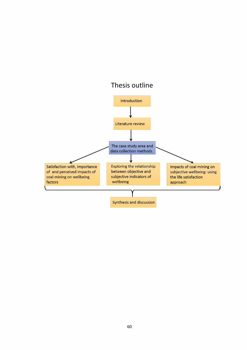
60

Thesis outline

61

3. CHAPTER 3 THE CASE-STUDY AREA AND DATA

COLLECTION METHODS

Chapter outline

3.1 Introduction

3.2 Coal mining in China

3.3 Shanxi province

3.4 Questionnaire Development

3.4.1 Questions for the questionnaire

3.4.2 Collection of data relating to objective wellbeing

3.4.3 Wording and sequencing questions

3.5 Data collection

3.5.1 Sampling framework

3.5.2 Survey implementation

3.5.3 Controlling survey errors

3.6 Sample overview

3.7 Conclusion

62

3.1 Introduction

To assess the ‘impact’ of coal mining on wellbeing, one needs to develop (a) a sampling

framework (deciding where, and from whom, one needs to collect data); and (b) a

questionnaire that will allow one to collect suitable data. As regards the sampling

framework: I chose to work within a region (Shanxi) where coal mining is prevalent and

important. Within that region, I chose to collect data in sub-regions with differential

exposures to coal mining so that I could compare results, and thus draw inferences

about the extent to which observed differences (in factors relating to wellbeing) were,

or were not, likely to be attributable to mining. As regards the questionnaire: the

literature discussed in the previous chapter clearly highlighted that wellbeing is a holistic

concept, and that to adequately measure it, one needs both objective and subjective

data – in addition to other contextual data (such as age and gender) known to be

associated with subjective assessments of wellbeing. I thus developed a comprehensive

survey focusing on subjective indicators; but sought to supplement that information

with other ‘objective’ data collected in the survey and elsewhere.

This chapter begins by providing some background information about the case-study

area, including a short history of government regulations relating to coal mining, the

problems associated with coal mining (section 3.2), and a description of Shanxi Province

(section 3.3). The development of the questionnaire is described in section 3.4. The

sampling framework and the process of data collection are presented in section 3.5,

followed by a sample overview in section 3.6. Importantly, this chapter only discusses

the general methods that are pertinent to the analyses presented in chapters 4, 5 and

6. Those other chapters also contain methodological discussions – but focus on the

methods that are specific to each.

3.2 Coal mining in China

Section 1.3.2 highlighted the fact that the relationship between resource development

and economic growth varies across countries. The relationship between resource-

dependence and wellbeing may vary also within regions or countries, as Stedman et al.

(2004) noted. Thus, investigations of coal mining and wellbeing should be based on

63

specific case studies. Social problems associated with coal mining in China are

characterised by the special history of government regulation.

From 1949 to 1994, state-owned enterprises (SOEs), which enjoyed large rents

generated by government-enforced monopolies, were the dominant players in the

mining sector (Wright, 2008; Zhang et al., 2008). These monopoly rents are the excess

income resulting from government regulation restricting the operation of the market.

Rent seeking is involved with the often legal efforts of enterprises or organizations to

create, maintain or oppose those monopoly rents, and the corrupt efforts by individual

bureaucrats to capture a part of those rents for themselves (Wright, 2008). Apparently,

these rents did not necessarily improve local welfare (Zhang et al., 2008).

Under the new regulations that were put in place after 1994, SOEs still enjoyed

preferential treatment in developing large mineral reserves, but local governments were

allowed to auction the development rights of small-scale mineral reserves left over by

the state sector to the private sector. As a result, many small-scale mines were privatized

and local governments enjoyed rents through their control over mining licences and

permits (Zhang et al., 2008).

Since 2009, the coal mining industry has undergone mergers and acquisitions through

government executive order. For example, in 2011, the total number of coal mines in

Shanxi was cut down by 60% as a result of the closure of small coal mines. After mergers

and acquisitions, new coal mines were operated by more than 130 companies, among

which state-owned or controlled companies accounted for more than 50% (Zhou, 2011).

Like many other developing countries, the mining regions of China suffer from

environmental and ecological problems caused by coal mining, and both the academic

circle and policy makers tend to devote most attention to the environmental impacts.

The social impacts of coal mining in China are paid relatively less attention, and very

little literature in China includes a comprehensive analysis of the multiple impacts of

mining, or provides empirical evidence of those impacts.

The benefits and burdens of coal mining in China have been distributed unevenly

geographically and socially. At the government level, the central government obtains a

64

higher proportion of tax and fees revenue from coal mining than local governments

(Zhao and Liu, 2011; Lei et al., 2013). At the individual level, coal mining enterprises and

individual bureaucrats who are involved with rent-seeking behaviour obtain most

benefit from coal mining, while local residents have been left bearing the brunt of the

negative externalities (Xu and Wang, 2006; Zhang et al., 2008; Zhao and Liu, 2011).

The unfair wealth distribution of resource development, and rent- seeking behaviour

can significantly widen the gap between the rich and poor (Xu and Wang, 2006). When

industry participants accumulate wealth, other local residents who are not able to share

the resource rent become relatively worse off (Xu and Wang, 2005; Shao and Qi, 2008).

Resource dominant economies also restrain the accumulation of human capital and the

development of science and technology (Xu and Wang, 2005). Zhan et al. (2015)

empirically found that resource dependence reduces government expenditure on

human capital. While most of the compensation for coal mining areas is limited to

control of environmental pollution and recovery of ecology, the impact on the quality of

life experienced in mining communities through, for example, changes in the

distribution of income, or changes to social capital has not been given much recognition

to date (Zhao and Liu, 2011).

3.3 Shanxi province

Shanxi was selected as the case-study area, as it is the most important province for coal

production, transportation, export and energy and chemical production (China Energy

Information Network, 2009).

The cumulative amount of coal resources identified in Shanxi ranks first in China,

accounting for 27% of the whole country. This is despite the fact that Shanxi accounts

for just 1.6% of China’s total land mass. About 40% of land in the whole province

contains coal (China Energy Information Network, 2010). The coal industry is not only

the main contributor to local GDP (Editor of Land & Resource Herald, 2013), but coal

from Shanxi also plays a significant role in the whole country, being exported to 26 out

of 30 of China’s province (Statistical Yearbook of Shanxi, 2014). It remained the largest

and the most important coal producer until 2009, being replaced by Inner-Mongolia

65

afterwards. In 2014, Shanxi produced the biggest yield of coal again, accounting for 25%

of coal production in China. During that year, 66% of the coal produced in Shanxi was

exported (Ma, 2014). China is in need of coal to fuel its economy. So the fact that coal

resource development dominates Shanxi economy will not change in short term.

The impacts of coal mining in Shanxi are typical of impacts reported throughout the

world. The industry is a two-edged sword. According to the list released by China's

environmental watchdog in 2004, Linfen, Yangquan and Datong – all cities within the

Shanxi Province – stood out on the black list (Qin, 2004). Since then, Linfen has been

cited as one of the most polluted places in China (e.g. Blacksmith Institute, 2007; Green

Forward News, 2014). Apart from having a substantive coal mining industry since 1978,

the numerous of private (illegal) mines within the Shanxi province is problematic; illegal

mines are some of the biggest polluters, as they do not follow any government

regulations (Green Forward News, 2014).

Since the consolidation of coal mining industry (after 2009), management and

supervision from government have been enhanced. Also, the government has put in

efforts to address environment problems by, for example, shutting down highly

polluting factories, and managed to reduce pollution. Linfen, consequently, is no longer

considered to be the “most polluted place on the Earth” (Official Website of China

National Radio, 2010).

Shanxi is a large province with a large population (see Table 3.1). Sampling across the

whole province would have been difficult and problematic, because there are

substantive differences between regions. Most notably are differences in language

(dialect): it would have been almost impossible to find research assistants who could

speak all of the dialects used in Shanxi Province. I thus focused on three regions:

Shuozhou, Yangquan and Linfen (highlighted in Figure 3.1). This selection was based on

the following considerations: first, they are located in the northern, central and southern

parts of Shanxi province, thus providing diverse geographic coverage. Second, these

areas play important and active roles as coal producers. Shuozhou produces most coal

and has the largest identified reserves; in terms of forecast reserves, Linfen ranks first

(China Coal Information, 2013). Third, compared to other areas, the industries of

66

Shuozhou and Yangquan are relatively homogeneous ─ with coal production and

electricity being the two main industries (see Table 3.2). Evidently, residents of these

regions have had some exposure to coal mining, processing and transportation, and are

thus likely to be in a good position to comment upon its impacts.

Figure 3.1 Map of Shanxi province

Table 3.1 Area and population of case-study areas (2013)

District Area (Km2) Population

Shuozhou 10662 1,744,169

Yangquan 4451 1,386,030

Linfen 20589 4,390,837

Shanxi 156,000 36,298,019

Source: From Shanxi Bureau of Statistics (2014).

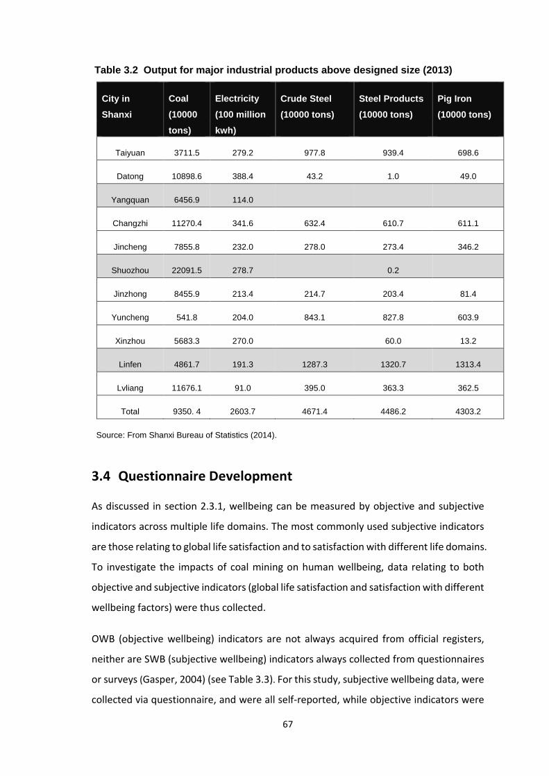
67

Table 3.2 Output for major industrial products above designed size (2013)

City in Shanxi

Coal (10000 tons)

Electricity (100 million kwh)

Crude Steel (10000 tons)

Steel Products (10000 tons)

Pig Iron (10000 tons)

Taiyuan 3711.5 279.2 977.8 939.4 698.6

Datong 10898.6 388.4 43.2 1.0 49.0

Yangquan 6456.9 114.0

Changzhi 11270.4 341.6 632.4 610.7 611.1

Jincheng 7855.8 232.0 278.0 273.4 346.2

Shuozhou 22091.5 278.7 0.2

Jinzhong 8455.9 213.4 214.7 203.4 81.4

Yuncheng 541.8 204.0 843.1 827.8 603.9

Xinzhou 5683.3 270.0 60.0 13.2

Linfen 4861.7 191.3 1287.3 1320.7 1313.4

Lvliang 11676.1 91.0 395.0 363.3 362.5

Total 9350. 4 2603.7 4671.4 4486.2 4303.2

Source: From Shanxi Bureau of Statistics (2014).

3.4 Questionnaire Development

As discussed in section 2.3.1, wellbeing can be measured by objective and subjective

indicators across multiple life domains. The most commonly used subjective indicators

are those relating to global life satisfaction and to satisfaction with different life domains.

To investigate the impacts of coal mining on human wellbeing, data relating to both

objective and subjective indicators (global life satisfaction and satisfaction with different

wellbeing factors) were thus collected.

OWB (objective wellbeing) indicators are not always acquired from official registers,

neither are SWB (subjective wellbeing) indicators always collected from questionnaires

or surveys (Gasper, 2004) (see Table 3.3). For this study, subjective wellbeing data, were

collected via questionnaire, and were all self-reported, while objective indicators were

68

either self-reported by respondents or observed by investigators (see highlighted part

in Table 3.3).

Table 3.3 Refined terms for subjective/objective wellbeing

Self-report indicators Non self-report (subject–independent) indicators

Measure of SWB ‘Self-report subjective’(e.g.: ‘I am

very satisfied with how far I can

walk’)

E.g. monitoring of types of brain function

and physiological indicator that express

SWB

Measure of OWB ‘Self-report objective’ (e.g.: ‘I can

walk 100 metres’) ‘Objective’─ observing how far people

really (can) walk, etc.

Source: From ‘Human well-being: concepts and conceptualizations’ (Gasper, 2004, p. 10).

Note: Highlighted parts are measures used in this study.

3.4.1 Questions for the questionnaire

The questionnaire included questions that are broadly grouped into three categories:

1) Questions about respondents’ perceptions

This includes their perception about their own wellbeing, what they think is important

to their wellbeing and how coal mining affects their wellbeing.

2) Questions about respondents’ characteristics

These questions refer to sociodemographic information, such as age, employment

status, marital status etc.

3) Questions about objective indicators

These questions refer to a few objective indicators, such as family income and whether

respondents have a bathroom or flushing toilet in their houses. This category will be

presented in detail in the following section.

69

3.4.1.1 Question about respondents’ perceptions

• Questions about overall life satisfaction

There are numerous ways of measuring global life satisfaction (GLS). Generally, these

approaches are classified into three (Hsieh, 2003), namely those: (1) using a number of

multiple-item life satisfaction measures (e.g. Satisfaction with Life Scale (SWLS) by

Diener et al. (1985)) (2) using a single-item question to evaluate life satisfaction (e.g.

Cantril ladder by Cantril (1965)) (3) summing satisfaction scores that have been

attributed to questions relating to individual life domains (e.g. Campbell et al., 1976).

The third approach is questioned by some researchers. Hsieh (2003) argued that the

extent to which summing across satisfaction within various domains represents GLS is

unclear. Fugl-Meyer et al. (1991) argued that GLS may be greater or less than the sum

of domain-specific satisfactions, and using a single measure of global satisfaction and

separate measures of domain-specific satisfaction would be a better choice.

This study followed that advice. Two different approaches were used to measure GLS ─

the scale of 0 to 100 measument similar to Cantril Ladder (Cantril, 1965) and Satisfaction

With Life Scale (SWLS) (Diener et al., 1985). In the Cantril ladder, people are asked to

rate how they value their life in terms of the best possible life (10) through to 0 (the

worst possible life). The International wellbeing group (2013), who has developed the

Personal Wellbeing Index, argues that converting the scale of 0 to 10 to the scale of 0 to

100, does not alter the statistical properties of the data, but offers the advantage that

wellbeing Index data can be directly compared to data of other scales used to measure

life satisfaction in terms of their means and standard deviations. Therefore, a scale from

0 to 100 is used in this study instead of 0-10. In SWLS, respondents are asked to express

their agreement on 5 statements about subjective wellbeing with a seven point scale

(Diener et al., 1985). The final score of SWLS is the sum of score from each question.

• Wellbeing factors across multiple domains selected for the questionnaire

As discussed in section 2.3.3, there is no commonly agreed set of ‘domains’ about which

researchers and organisations who are interested in wellbeing regularly collect data.

Davey and Rato (2012) encouraged the use of diverse and creative measures; different

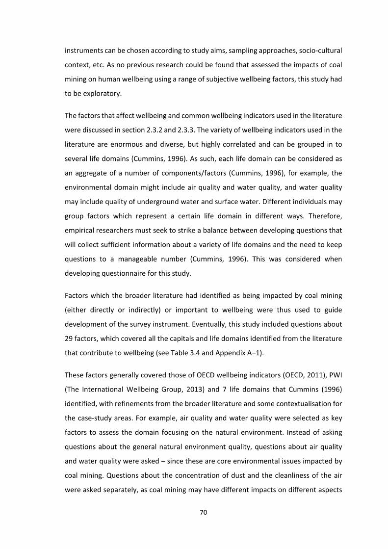
70

instruments can be chosen according to study aims, sampling approaches, socio-cultural

context, etc. As no previous research could be found that assessed the impacts of coal

mining on human wellbeing using a range of subjective wellbeing factors, this study had

to be exploratory.

The factors that affect wellbeing and common wellbeing indicators used in the literature

were discussed in section 2.3.2 and 2.3.3. The variety of wellbeing indicators used in the

literature are enormous and diverse, but highly correlated and can be grouped in to

several life domains (Cummins, 1996). As such, each life domain can be considered as

an aggregate of a number of components/factors (Cummins, 1996), for example, the

environmental domain might include air quality and water quality, and water quality

may include quality of underground water and surface water. Different individuals may

group factors which represent a certain life domain in different ways. Therefore,

empirical researchers must seek to strike a balance between developing questions that

will collect sufficient information about a variety of life domains and the need to keep

questions to a manageable number (Cummins, 1996). This was considered when

developing questionnaire for this study.

Factors which the broader literature had identified as being impacted by coal mining

(either directly or indirectly) or important to wellbeing were thus used to guide

development of the survey instrument. Eventually, this study included questions about

29 factors, which covered all the capitals and life domains identified from the literature

that contribute to wellbeing (see Table 3.4 and Appendix A–1).

These factors generally covered those of OECD wellbeing indicators (OECD, 2011), PWI

(The International Wellbeing Group, 2013) and 7 life domains that Cummins (1996)

identified, with refinements from the broader literature and some contextualisation for

the case-study areas. For example, air quality and water quality were selected as key

factors to assess the domain focusing on the natural environment. Instead of asking

questions about the general natural environment quality, questions about air quality

and water quality were asked – since these are core environmental issues impacted by

coal mining. Questions about the concentration of dust and the cleanliness of the air

were asked separately, as coal mining may have different impacts on different aspects

71

of air quality. Questions about “spirituality and religion” were not included, as in this

area residents are not generally religious.

72

Table 3.4 Selected wellbeing factors according to the literature

Selected wellbeing factors Literature about the impacts of coal mining on wellbeing factors

Literature that illustrate that these factors have effect on wellbeing

Broad wellbeing factors in the literature

Refinded factors in this study

Air quality (Bian et al., 2010; Zullig and

Hendryx, 2010, 2011; Colagiuri et

al., 2012)

(Welsch, 2006, 2007a; MacKerron and Mourato, 2009; Ferreira and

Moro, 2010; Menz and Welsch, 2010; Levinson, 2012; Cuñado and

de Gracia, 2013), air and water pollution (Welsch, 2002; Luechinger,

2009), noise pollution (van Praag and Baarsma, 2005)

Water quality and access (Guardiola et al., 2013)

Surface water

Health

Physical health

(Bian et al., 2010; Zullig and

Hendryx, 2010, 2011; Colagiuri et

al., 2012)

(Winkelmann and Winkelmann, 1998; Frey and Stutzer, 1999b; Frey

and Stutzer, 2002a; Di Tella et al., 2003; Groot and Maassen van den

Brink, 2003; Helliwell, 2003; Ferrer‐i‐Carbonell and Frijters, 2004;

Winkelmann, 2005; Seghieri and Desantis, 2006; Ferrer-i-Carbonell

and Gowdy, 2007; Brereton et al., 2008; Rehdanz and Maddison,

2008; Luechinger, 2009; MacKerron and Mourato, 2009;

Powdthavee, 2010; Ambrey and Fleming, 2011; Levinson, 2012;

Cuñado and de Gracia, 2013; Ambrey and Fleming, 2014a)

Mental Health (Krannich and Greider, 1984)

73





Education

Quality of

education system

and oppoortunity

for education

(Gylfason, 2001; Gylfason and

Zoega, 2006; Zhan et al., 2015)

(Frey and Stutzer, 2000, 2002a; Di Tella et al., 2003; Groot and

Maassen van den Brink, 2003; Helliwell, 2003; Alesina et al., 2004;

Seghieri and Desantis, 2006; Ferrer-i-Carbonell and Gowdy, 2007;

Welsch, 2007b; Abdallah et al., 2008; Brereton et al., 2008; Michalos,

2008; Ebert and Welsch, 2009; Luechinger and Raschky, 2009;

Stanca, 2009; Powdthavee, 2010; Stanca, 2010; Ambrey and

Fleming, 2011; Arifwidodo and Perera, 2011; Kountouris and

Remoundou, 2011; Beja Jr, 2012; Levinson, 2012; Beja Jr, 2013;

Cuñado and de Gracia, 2013; Ambrey and Fleming, 2014b, a)

Relationship Personal/family

relationship None Cummins (1996)

Social capital

Participation of

social activity

(Kitula, 2006; Lockie et al., 2009;

Carrington et al., 2011)

Trust (Helliwell, 2003; Engelbrecht, 2009; MacKerron and Mourato, 2009;

Stanca, 2009, 2010; Bartolini and Sarracino, 2011) Help

Honesty

Perceived safety Personal safety (Michalos and Zumbo, 2000)

Property safety

Quality of government (Sachs and Warner, 1999, 2001;

Gylfason and Zoega, 2006) (Abdallah et al., 2008; Helliwell and Huang, 2008)

74





Income

Individual income (Carrington,

Hogg et al., 2011); Regional GDP

(National Mining Association, 2014; Editor of Land & Resource Herald,

2013)

(Frijters and Praag, 1998; Winkelmann and Winkelmann, 1998;

Diener et al., 1999; Frey and Stutzer, 1999b; Cummins, 2000; Frey

and Stutzer, 2000; Michalos and Zumbo, 2000; Easterlin, 2001; Frey

and Stutzer, 2002a; Welsch, 2002; Di Tella et al., 2003; Groot and

Maassen van den Brink, 2003; Helliwell, 2003; Ferrer‐i‐Carbonell

and Frijters, 2004; Rehdanz and Maddison, 2005; Winkelmann,

2005; Seghieri and Desantis, 2006; Welsch, 2006; Ferrer-i-Carbonell

and Gowdy, 2007; Welsch, 2007b; Abdallah et al., 2008; Brereton et

al., 2008; Inglehart et al., 2008; Rehdanz and Maddison, 2008; Smyth

et al., 2008; Carroll et al., 2009; Engelbrecht, 2009; Luechinger,

2009; Luechinger and Raschky, 2009; MacKerron and Mourato,

2009; Stanca, 2009; Ferreira and Moro, 2010; Menz and Welsch,

2010; Powdthavee, 2010; Stanca, 2010; Ambrey and Fleming, 2011;

Kountouris and Remoundou, 2011; Beja Jr, 2012; Levinson, 2012;

Beja Jr, 2013; Cuñado and de Gracia, 2013; Ambrey and Fleming,

2014a, b). Relative income studied by (Daly, 1987; Easterlin, 1995;

Dixon, 1997; Diener et al., 1999; Easterlin, 2003b; Layard, 2003;

Stutzer and Frey, 2010)

Income disparity (Xu and Wang, 2006; Zhang et al.,

2008; Zhao and Liu, 2011)

(Daly, 1987; Easterlin, 1995; Dixon, 1997; Diener et al., 1999;

McBride, 2001; Easterlin, 2003b; Layard, 2003; Stutzer and Frey,

2010) Fairness of income

75





Price

Price of

necessities and

real estate (Carrington et al., 2011) (Di Tella, MacCulloch et al. 2001, Engelbrecht 2009)

Inflation rate

Housing

Land subsidence might cause

damage to house (Bian et al.,

2010); Improve living conditions

(Zhang et al., 2015)

(Marans, 2003; OECD, 2011)

Electricity (International Energy Agency,

2016)

(Cousins, 1998; Karekezi, 2002; Pachauri and Spreng, 2004;

Kammen and Kirubi, 2008)

Transportation and communication

(Australians for Coal, 2014; Coal

Association of Canada, 2011;

Zhang et al., 2015)

(Brereton et al., 2008)

Note: The column “Literature that illustrate that these factors have effect on wellbeing” was selected from ‘The impact of economic, social and environmental factors on trip satisfaction and the likelihood of visitors returning’ (Jarvis et al., 2016, p. 14-16).

76

• Questions about satisfaction with wellbeing factors

The OECD (2013) argues that a longer (7 to 11 point) scale is better than a short (2 to 5

point) scale for single item measures of life satisfaction (satisfaction with wellbeing

factors). In addition, many existing and widely-used scales for life evaluations are bipolar

(running between two opposing constructs, i.e. from completely unhappy to completely

happy) instead of unipolar (i.e. reflecting a single construct running from low to high),as

bipolar scale anchors may be the least ambiguous in terms of all respondents

interpreting the scale in the same way. Therefore, this study used a bipolar scale, with a

score from 1 (strongly dissatisfied) to 7 (strongly satisfied), to measure satisfaction with

different wellbeing factors (see Table 3.5).

• Questions about importance of wellbeing factors

In addition to asking respondents to indicate their level of satisfaction with particular

wellbeing factors, the study also included questions asking about their importance. To

align with the scale used to measure satisfaction with wellbeing factors, a 7-point scale

was used to assess importance, ranging from very important (7) to very unimportant (1)

(see Table 3.5).

Hsieh (2003) empirically proved that using discrete domain importance rating as a

weighting factor did not improve the correlation between GLS measure and satisfaction

with wellbeing factors, while the correlation was improved by using ranking of

importance. As such, this study did not use importance scores to weight satisfaction

scores in an overall regression explaining GLS. Instead, the importance scores were used

to try and understand if those living in the different case-study areas had inherently

different opinions about what is, or is not, important in life.

• Questions of coal mining impacts on particular factors

According to Stedman et al. (2004), the relationship between resource-dependence and

wellbeing may vary between regions and industries. While impacts of coal mining on the

natural environment are well discussed in the literature and have something in common,

the social impacts may vary across countries and regions. Based on the particular

economic and political climate described in section 3.2, the social impact of coal mining

77

in China might be unique. Thus, the study also sought to learn more about people’s

perceptions of the impacts of coal mining, addressing the research gaps identified in

section 2.5.4. For each of the 29 factors about which information on ‘satisfaction’ and

‘importance’ was collected, I also sought information on ‘impact’. To align with the

scales used on those indicators, a 7-point scale was used to assess the impact of coal

mining on each wellbeing factor, ranging from a strong negative impact (1) to a strong

positive impact (7) (see Table 3.5).

Table 3.5 Scales used in the questionnaire

Global life

satisfaction

LS 0–100 SWLS

1 2 3 4 5 6 7

Strongly

disagree Disagree

Slightly

disagree Neutral

Slightly

agree Agree

Strongly

agree

Satisfaction with wellbeing factors

Very

dissatisfied Dissatisfied

Slightly

dissatisfied Neutral

Slightly

satisfied Satisfied

Very

satisfied

Importance of wellbeing factors

Very

unimportant Unimportant

Slightly

unimportant Neutral

Slightly

important Important

Very

important

Coal mining’s impacts on wellbeing factors

Strongly

negative Negative

Slightly

negative

No

impact

Slightly

positive Positive

Strongly

positive

3.4.1.2 Questions about sociodemographic characteristics

Most wellbeing studies also include questions about various sociodemographic

characteristics that have been shown to influence subjective wellbeing. Table 3.6 is a

summary of the list of the relevant sociodemographic characteristics from literature.

Following the lead of previous research, this study thus also included questions about

respondents’ age, gender, marital status, education level, employment status, family

size (number of children and adults).

78

Table 3.6 Sociodemographic variables found to be significant in explaining overall life satisfaction

Explanatory variable

Studies where sociodemographic variable found to be significant in explaining overall satisfaction with life

Age

(Oswald, 1997; Frijters and Praag, 1998; Winkelmann and Winkelmann, 1998; Frey and Stutzer, 1999a, 2000; Michalos and Zumbo, 2000; Frey and Stutzer, 2002a; Di Tella et al., 2003; Groot and Maassen van den Brink, 2003; Helliwell, 2003; Alesina et al., 2004; Ferrer‐i‐Carbonell and Frijters, 2004; van Praag and Baarsma, 2005b; Winkelmann, 2005; Seghieri and Desantis, 2006; Ferrer-i-Carbonell and Gowdy, 2007; Welsch, 2007b; Brereton et al., 2008; Rehdanz and Maddison, 2008; Smyth et al., 2008; Carroll et al., 2009; Ebert and Welsch, 2009; Luechinger, 2009; Luechinger and Raschky, 2009; MacKerron and Mourato, 2009; Stanca, 2009; Menz and Welsch, 2010; Powdthavee, 2010; Stanca, 2010; Ambrey and Fleming, 2011; Kountouris and Remoundou, 2011; Beja Jr, 2012; Levinson, 2012; Beja Jr, 2013; Cuñado and de Gracia, 2013; Ambrey and Fleming, 2014b, a)

Gen

der

(Frey and Stutzer, 1999a; Michalos and Zumbo, 2000; Groot and Maassen van den Brink, 2003; Alesina et al., 2004; Winkelmann, 2005; Seghieri and Desantis, 2006; Ferrer-i-Carbonell and Gowdy, 2007; Welsch, 2007b; Brereton et al., 2008; Rehdanz and Maddison, 2008; Carroll et al., 2009; Ebert and Welsch, 2009; Luechinger and Raschky, 2009; Stanca, 2009; Powdthavee, 2010; Stanca, 2010; Levinson, 2012; Beja Jr, 2013; Ambrey and Fleming, 2014a)

Mar

ital s

tatu

s

(Winkelmann and Winkelmann, 1998; Diener et al., 1999; Frey and Stutzer, 1999a, 2000; Michalos and Zumbo, 2000; Frey and Stutzer, 2002a; Groot and Maassen van den Brink, 2003; Helliwell, 2003; Alesina et al., 2004; Ferrer‐i‐Carbonell and Frijters, 2004; Seghieri and Desantis, 2006; Ferrer-i-Carbonell and Gowdy, 2007; Welsch, 2007b; Rehdanz and Maddison, 2008; Carroll et al., 2009; Ebert and Welsch, 2009; Luechinger, 2009; Luechinger and Raschky, 2009; MacKerron and Mourato, 2009; Stanca, 2009; Ferreira and Moro, 2010; Powdthavee, 2010; Stanca, 2010; Arifwidodo and Perera, 2011; Kountouris and Remoundou, 2011; Beja Jr, 2012; Levinson, 2012; Beja Jr, 2013; Cuñado and de Gracia, 2013; Ambrey and Fleming, 2014b, a)

Educ

atio

n le

vel Relationship found by (Frey and Stutzer, 2000, 2002a; Groot and Maassen van den Brink, 2003;

Helliwell, 2003; Alesina et al., 2004; Seghieri and Desantis, 2006; Ferrer-i-Carbonell and Gowdy, 2007; Welsch, 2007b; Abdallah et al., 2008; Brereton et al., 2008; Ebert and Welsch, 2009; Luechinger and Raschky, 2009; Stanca, 2009; Powdthavee, 2010; Stanca, 2010; Ambrey and Fleming, 2011; Arifwidodo and Perera, 2011; Kountouris and Remoundou, 2011; Beja Jr, 2012; Levinson, 2012; Beja Jr, 2013; Cuñado and de Gracia, 2013; Ambrey and Fleming, 2014b, a).

Empl

oyed

or

unem

ploy

ed (Winkelmann and Winkelmann, 1998; Frey and Stutzer, 1999a; Helliwell, 2003; Alesina et al., 2004;

Winkelmann, 2005; Seghieri and Desantis, 2006; Ferrer-i-Carbonell and Gowdy, 2007; Welsch, 2007b; Brereton et al., 2008; Rehdanz and Maddison, 2008; Smyth et al., 2008; Ebert and Welsch, 2009; Luechinger, 2009; Luechinger and Raschky, 2009; Stanca, 2009; Ferreira and Moro, 2010; Powdthavee, 2010; Stanca, 2010; Beja Jr, 2012; Levinson, 2012; Beja Jr, 2013; Cuñado and de Gracia, 2013; Ambrey and Fleming, 2014a)

Fam

ily

size

(Frijters & van Praag, 1998; Frey & Stutzer, 2000; Di Tella, MacCulloch, & Oswald, 2003; Moro, Brereton, Ferreira, et al., 2008; Stutzer & Frey, 2008)

Source: Selected from ‘The impact of economic, social and environmental factors on trip satisfaction and the likelihood of visitors returning’ (Jarvis et al., 2016, p. 14-16).

79

3.4.2 Collection of data relating to objective wellbeing

Although some data about objective wellbeing were available from various government

departments, the data tendered to be aggregated over higher administrative levels than

the scale required by the research question (reported, for example, at whole of county

rather than village level). Thus, objective data also needed to be collected for this study.

It was not financially feasible to collect objective wellbeing indicators for all the 29

factors, but the OECD “Framework for OECD wellbeing indicators” (see Figure 2.2), was

used to guide the construct of the survey, collecting information about a variety of

factors relating to material conditions ─ e.g. family income, housing (room per person,

the existence of bathroom and flushing toilet) ─ and to quality of life (e.g. employment

status, education level). Most objective data were thus reported by individuals and

collected using questionnaires (see Appendix A–1), while data relating to air quality

(which are difficult for individuals to measure and thus report on) were measured by the

investigators using a hand-held air-quality monitor during the study. Specifically,

researchers recorded the concentration of 8PM2.5 and PM10 at each sampling location.

This measurement cannot be extrapolated to indicate average annual air quality, as the

air quality is expected to vary with wind direction and strength and is subject to seasonal

fluctuation. It is only presented as an indicator relative to other respondents and study

sites.

3.4.3 Wording and sequencing questions

3.4.3.1 Wording of questions

The actual wording of the questionnaire is crucial. In this case, the survey was targeted

at the general population, which means the potential respondents could have been any

adult of any age and education level. Therefore, it was important that every single

question could be understood easily without being explained.

8 PM (particle matter) refers to an air pollutant which has adverse effects on human health (Dockery et al., 1993). The degree of PM pollution is frequently assessed by continuous monitoring of the levels of PM10 and PM2.5. PM10 is particulate matter with aerodynamic size 10 μm or less, while PM2.5 is particulate matter with aerodynamic size 2.5 μm or less (RODRıGUEZ et al., 2004).

80

The following checklist of general principles (Dillman, 1978, Salant and Dillman, 1994,

and DeVellis, 2003, cited by Larson, 2010, p. 74) was used as a guideline on wording the

questionnaires.

Will the words be uniformly understood? Is the questionnaire objective?

Are the questions too vague? Too precise? Too cryptic? Too demanding?

Are the questions biased? Is the questionnaire technically accurate?

3.4.3.2 The sequence of questions

Some researchers suggested that sociodemographic questions about respondents, such

as age, marital status, education level and income, should be asked at the end of

questionnaire instead of the beginning to avoid the impact of any negative feelings on

the answer behaviour and participation (Converse and Presser, 1986; Oppenheim, 1992).

Thus, sociodemographic questions came at the end of this questionnaire.

The ‘order effect’ of questions refers to the fact that relative position of an item in an

inventory of questions may uniquely influence the way in which a respondent reacts to

the item (Perreault, 1975). Order effect could be controlled by producing different

questionnaires, comprised of random orderings of relevant items (while maintaining

proper overall sequence) (Perreault, 1975). Therefore, the sequence of the questions

were regularly changed, except the demographic questions. Two measurements of GLS

were located at the beginning and end of the questionnaire separately ─ SWLS was

located at the beginning of the questionnaire to allow respondents to give their own

first–impression evaluation, while the question about LS using scale of 0 – 100 was

located at the end to allow respondents to evaluate their GLS after they had got through

the evaluation of all the life domains.

3.4.3.3 Translation between Mandarin and English

The questionnaire was originally designed in English. It had to be translated into

Mandarin because the potential respondents only speak Mandarin or a local dialect.

Following Chen and Lin (2014), the questionnaire was firstly forward translated into

81

Mandarin by the author, then a backward translation was conducted by a different

translator who had never seen the original survey questions. The backward translation

was checked against the original to ensure there were no discrepancies between them.

3.4.3.4 Pilot testing

1) Expert testing

The expert group consisted of academic researchers, who had professional knowledge

about wellbeing and the impacts of coal mining and experience about questionnaire

design. They understood the purpose of this study and questionnaire better than other

randomly selected respondents. Scientific merit, the relevance of the data collected,

wording and layout of the questionnaire were discussed by this group. The

questionnaire was improved in terms of clarity, scientific quality and accuracy after this

process.

2) Sub-sample testing

Sub-sample testing was conducted to make sure the questionnaire was practicable.

About 15 face to face interviews were performed during the pilot stage of this project.

Not all of them were from coal mining areas or aware of the impacts of coal mining.

However, they still helped to improve the questionnaire. The verbal feedback was

collected, and signs of hesitation, confusion and discomfort when respondents

answered the questions were observed. The questionnaire was tested for wording,

understanding, and sequence of questions. The following checklist was used as a

guideline to amendments on the draft questionnaire at the pilot stage (Dillman, 1978

and Salant and Dillman, 1994, cited by Larson, 2010, p. 75).

Are questions interpreted similarly by all respondents?

Are questions answered correctly (are some missed or elicited uninterpretable answers)?

Does each closed – ended question have an answer that applies to each respondent?

Does any aspect of the questionnaire suggest bias on the part of the researcher?

82

As a result of the pilot testing, some amendments were made to improve the

questionnaire. Some of the questions were clarified, some relatively unimportant

questions were deleted to shorten the questionnaire, and some wording was changed

to make the questionnaire easier to understand. The layout and structure of the

questionnaire were also modified according to respondents’ suggestions.

3.5 Data collection

3.5.1 Sampling framework

As discussed in section 2.5.6, few previous studies that have looked at impacts of coal

mining have compared impacts in regions with different intensities of coal mining. The

literature strongly suggests that LS studies should consider geography – looking, for

example, at urban or rural areas, or places that share similar environmental

characteristics. As such, an investigation into the impacts of coal mining on life

satisfaction/wellbeing should involve the comparison between places with different

intensities of coal mining. Previous literature offers some clues about how to

differentiate regions according to mining intensities. Kitula (2006) simply compared coal

mining areas and non-coal mining areas. Hendryx and Ahern (2009) divided Appalachia

with high levels of coal mining, Appalachia with lower mining levels, Appalachia without

coal mining, and other counties in the nation. Regions were classified as being ‘high’ or

‘low’ intensity according to coal production. The CSIRO studies compared mining regions,

non-mining regions, and other metropolitan areas (Moffat et al., 2014a; Moffat et al.,

2014b; Zhang et al., 2015).

Counties in Shanxi Province, like many other provinces in China, have a large population,

and contain a large number of villages. The diversities between the villages inside a

county are dramatic: in a single county, there are villages immediately adjacent to coal

mines and those relatively close to coal mines. Sampling of communities was stratified

by distance on a scale of an average 10 kilometres of coal mining operations as detailed

in Table 3.7. I also chose to differentiate between urban and rural areas because there

are significant differences between lifestyles, livelihoods, and incomes in rural and

83

urban areas of China (Yang and Cai, 2003; Lu and Chen, 2004; Kanbur and Zhang, 2005;

Sicular et al., 2007) .

Information on distribution of coal mining was collected from local governments,

various media outlets (e.g. websites) and via informal communications with local people.

Study sites were identified within a general region that would allow a differentiation

between places according to their proximity to coal mines. Reconnaissance of the study

area revealed that: coal extraction (mining) in these areas was typically closely

associated and often co-located with coal stockpiles, transportation routes and coal

washing facilities, all of which, alone or in combination, would impact local residents’

lives. Therefore, this study considered their variously combined impacts as the

aggregated impacts of coal mining.

84

Table 3.7 Criteria for selecting sampling sites that represent different intensities of coal mining

Classification category

Defined as

Place with coal mining

Coal mining, with or without associated activities/facilities (such as coal

washing and coal transportation), present within 10km of the

administrative/residential area and present high-intensity exposure to

impacts of coal mining.

Place close to coal mining

Coal mining, with or without associated activities/facilities, present within

10–20 km of the administrative residential area and present moderate-

intensity exposure to impacts of coalmining.

Place far from coal mining

Coal mining, with or without associated activities/facilities, absent within

20 km of the administrative/residential area and presenting none or only

light exposure to coal mining impacts.

As the access to urban facilities or major transport routes might have effect on quality

of life (Brereton et al., 2008; Arifwidodo and Perera, 2011), villages were selected at

similar distances from urban areas to minimize this effect. Coal mining is not allowed in

the urban area. Therefore, 5 types of case-study region (see Figure 3.2) were identified,

including rural area with coal mining (Rural With), rural area close to coal mining (Rural

Close), urban area close to coal mining (Urban Close), urban areas far from coal mining

(Urban Far) and rural area far from coal mining (Rural Far). The phrases “5/different

(types of) study regions/ areas” and “regions/ areas/places with different intensities of

coal mining” are used in the rest of this thesis, to refer to these 5 different types. The

phrases “coal mining areas/regions” refers to Urban Close, Rural With and Rural Close,

while “non-coal mining areas” refers to Urban Far and Rural Far.

85

Figure 3.2 Different types of study region Note: White circles indicate the location of coal mines.

Source: Pictures for Urban Far, Rural Far and Rural Close are screen shots from Google Map; The picture for Rural With was taken by investigator on 22th August, 2013; The picture for Urban Close is from the internet9, accessed on 15th March 2015.

3.5.2 Survey implementation

Research assistants, who were university students and spoke the local dialect, were

trained at a one day workshop. Research objectives, methods and interview techniques

were introduced to them. They were asked to practise the interview process with each

other. They went out in pairs to conduct the surveys by interview. Research assistants

filled out the questionnaire according to the answers provided by respondents.

9 http://world.haiwainet.cn/n/2014/1015/c456832-21219345-11.html.

86

Various survey approaches were considered. A mail survey is impracticable in China,

because many households have no mail box, especially rural places. Door-to-door

household surveys are impracticable in urban areas, because most urban residents live

in apartments and are too suspicious to open their door for strangers. Thus in urban

areas, research assistants approached potential respondents on the streets or in places

such as public squares, parks, and shops. In rural areas, a door-knock survey covering as

large an area as possible was conducted in each village. Places where local residents

collected for social interaction (such as public squares) were also visited for data

collection. Strategies used to control survey errors and data bias are discussed in the

following section.

In places with coal mining, people were more suspicious of the purpose of investigators.

They became willing to be interviewed once they observed other people being

interviewed and once they heard more about the exact questions asked. In places far

from coal mining, people were generally very willing to be interviewed.

The sampling framework had to be somewhat adjusted ‘in field’. For example, after

sampling two urban areas, it became apparent that these residents were virtually

unaffected by coal, so further sampling effort was focused on rural areas. Moreover, the

classification of villages selected for inclusion in the sample was adjusted after the

survey when more information was acquired. A village had a coal mine which was less

than 10 km from the village, but the coal mine was separated from the village by a hill.

Thus, the connection between the coal mine and the village was very weak. In this study,

this village was thus re-classified as “Rural area near (rather than with) coal”. The

following table provides details of the final sampling framework.

87

Table 3.8 Sampling of study regions

3.5.3 Controlling survey errors

It is necessary to consider how to reduce different types of survey error when

conducting a survey. Several common survey errors were considered in this study.

According to Dillman (1991), four potential sources of error should be considered:

sampling error, measurement error, non-coverage error and non-response error.

1) Sampling error

Sampling error is attributed to the fact that certain members of the population are

deliberately excluded by selection of the subset of members (Dillman, 1991). This survey

was designed to include respondents with diverse characteristics. When conducting

interviews, the diversity of respondents was able to monitored and controlled by

investigators, which helped control this error. Those who might not be able to make

sensible judgements were excluded in the survey, such as people who are under 16

years old, or people who could not express themselves very clearly.

10 Xiashe contains 12 relatively small and similar villages that closely connect to each other. These villages were considered as one location here.

Sampling area

Urban area Rural area Urban Close Urban Far Rural With Rural Close Rural Far

Area 1 – Shouzhou

Centre of area 1 Ciyu Zhaoshibazhuang

Pinglu district Damuguajie Wochang,

Kangjiayao

Yingxian

Xiashe ─

including

12

villages10

Area 2 – Xiangning

Centre of area 2 Hucun,

Jizhuanggou Zhangma

Area 3– Yangquan

Centre of area 3 Dacun, Banpo,

Jieshang

Houjiagou,

Changling

88

2) Measurement error

Measurement error may result from characteristics of the question or questionnaire.

Based on the literature, this questionnaire had been through a pilot test and

modification in order to reduce this error.

3) Non-coverage error and Non-response error

Non-coverage error arises because some members are not included by the sampling

frame and have no chance to be selected as the sample (Dillman, 1991), and non–

response error stems from the fact that a certain group of the members of the sample

population do not respond to the survey questions. To reduce these errors, we tried to

cover as large an area as possible in each place we visited to interview potential

respondents. We could not generate a ‘perfect’ stratified random sample, but as we

conducted interviews, we monitored and controlled the diversity of respondents to

identify and control these errors (e.g. specifically asking to interview a male, if relatively

few males had been interviewed in one area/day).

3.6 Sample overview

Table 3.9 shows the number of responses collected from different areas – with an

uneven number from each. The core interest of this study was to investigate the impacts

of coal mining on wellbeing in regions with different intensities of coal mining. So areas

without any mining at all were included for comparative purposes, but not covered in

detail. Rural areas involved with coal mining (either near or immediately adjacent to

mines) were the key interest of this study and account for the largest proportion of the

total sample. Social science research in China is somewhat limited in that most data have

been collected from urban samples, overlooking the rural residents who account for 60

of the total population (Davey and Rato, 2012). This study thus offers some insights

about the subjective wellbeing in rural areas, that are of interest beyond observations

relating to coal mining.

According to Cummins (1996), the utility of GLS measurement for comparison among

small groups is limited. Sample sizes for places far from coal mining are relatively small

89

(with just 59 individuals from 12 small villages that were classified as “rural far” and 30

individuals in regions classified as “urban far”), so the analytical approaches used in

subsequent chapters take that into account (using, for example, non-parametric

techniques ideally suited to small samples, and then focusing predominantly on the

larger sub-samples in other analyses).

Table 3.9 also provides summary statistics relating to the sociodemographic

characteristics of the sub-samples, compared to sociodemographic statistics collected

by Chinese data collection agencies for their census in the Shanxi province. Most evident,

is that the average family income of the urban samples is lower than the average family

income recorded in the census data. In contrast, the family income of the rural samples

is higher than that of census data. This indicates that it will be important to ensure that

the effect which income has on wellbeing is considered in the analyses of chapter 6, to

control for any potential bias that might arise if the sample is not representative of the

population as a whole. The sample also includes a disproportionate number of men

(compared to the census data), underscoring the importance of also attempting to

control of the influence of gender when assessing contributors to SWB. The fact that

incomes are higher for those who work for the coal mining industry than those who

work in other industries (and these differences are statistically significant in two regions:

Rural With and Rural Close), is consistent with census data (see Appendix B).

90

Table 3.9 Sample information

Urban Close

Rural With

Rural Close

Urban Far

Rural Far

Urban areas

Rural areas Total

Shanxi

Urban areas

Rural areas

Population from each Location 90 184 179 30 59 120 422 542 Percentage of Population from each location 16.6% 33.9% 33.0% 5.5% 10.9% 22.1% 78.0% 100% 32.7% 64.3%

Family income Average family income 50765 33800 32288 60000 31949 53174 32900 37266 67367 23893

Percentage of family income sourced from coal mining 14.8% 32.1% 16.2% 0.0% 0.0% 18.7%

Average family Income from coal mining industry 42895 39237 41071

Average family Income from non-coal mining industry 31667 31210 31084 Gender Percentage of male

42.2% 47.3% 35.8% 33.3% 35.6% 60.0% 59.2% 40.6% 51.4%

Percentage of female 57.8% 52.7% 64.2% 66.7% 64.4% 40.0% 40.8% 59.4% 48.6% Marital Status Percentage of partnered 58.9% 85.3% 85.5% 76.7% 84.7% 63.3% 85.3% 91.7%

Percentage of non-partnered 41.1% 14.7% 14.5% 23.3% 15.3% 36.7% 14.7% 8.3% Family size Average children per household 0.8 0.7 0.9 0.5 0.4 0.7 0.7 0.7

3.0 3.3 Average adult per household 3.2 3.3 3.2 3 3.3 3.1 3.3 3.2 Age

16–26

37.8% 11.7% 12.1% 23.3% 11.9% 34.2% 11.8% 16.8%

26–35

23.3% 22.9% 16.1% 20.0% 5.1% 22.5% 18.0% 19.0%

36–45

14.4% 16.8% 22.1% 16.7% 22.0% 15.0% 19.4% 18.5%

46–55

7.8% 23.4% 20.8% 13.3% 27.1% 9.2% 23.0% 19.9%

91

Urban Close

Rural With

Rural Close

Urban Far

Rural Far

Urban areas

Rural areas Total

Shanxi

Urban areas

Rural areas

56–65

5.6% 14.0% 19.5% 10.0% 20.3% 6.7% 16.8% 14.6%

Above 65

11.1% 11.2% 9.4% 16.7% 13.6% 12.5% 0.9% 11.3%

Education level Illiteracy or little literacy 6.7% 16.4% 20.8% 16.7% 33.9% 9.2% 20.4% 17.9%

Primary school 17.8% 44.9% 44.3% 20.0% 28.8% 18.3% 42.4% 37.1%

Junior Middle School 27.8% 23.4% 17.4% 13.3% 20.3% 24.2% 20.9% 21.6%

Level of Senior Middle School 26.7% 4.2% 3.4% 30.0% 6.8% 27.5% 4.3% 9.4%

Specialized Secondary School 3.3% 0.0% 0.0% 3.3% 0.0% 3.3% 0.0% 7%

Junior College and Above 17.78% 11.21% 14.09% 16.67% 10.17% 17.50% 12.09% 13.3% Employment status Self-employed 27.8% 37.4% 46.3% 16.7% 44.1% 25.0% 41.5% 37.8%

Has job 31.1% 23.4% 28.5% 40.0% 22.0% 33.4% 25.3% 27.1%

Jobless 13.3% 27.6% 17.3% 13.4% 10.0% 18.6% 22.5% 19.4%

Student 20.0% 3.3% 4.5% 16.7% 5.1% 19.2% 4.0% 7.4%

Retired 7.8% 6.1% 9.4% 16.7% 10.2% 10.0% 7.80% 8.3%

Notes: 1. Data for the entire Shanxi are extracted from Shanxi Bureau of Statistics (2014); Some data aligned with this study are missing because they are not available in the Yearbook or not comparable due to different measurements; 2. Average individual income is available in the yearbook instead of family income, thus average family income of Shanxi was roughly calculated as following:

Family income of urban areas=Average household size *total income per capital of urban households = 3.0*22455.63 ≈ 67367

Family income of rural areas= Average Household Size *total income per capital of urban households = 3.3*7153.50 ≈ 23893

92

3.7 Conclusion

To investigate the impacts of coal mining on wellbeing, areas characterized with

different intensities of coal mining (based on the distance of coal mining) were identified

(these included Rural With, Rural Close, Urban Close, Urban Far and Rural Far) and data

were collected from each type of area (albeit focusing on those ‘with’ and ‘close to’ coal

mines, to draw out the intensities issue).

This study collected subjective, objective and sociodemographic data. Questions of

subjective wellbeing included global life satisfaction and satisfaction with 29 wellbeing

factors. Data relating to people’s subjective perceptions about the importance of each

factor to their overall wellbeing and their perception of the impacts of coal mining on

those factors were also collected. Data relating to objective indicators were also

collected, including that relating to material conditions (family income, rooms per

person, the existence of bathroom and flushing toilet) and other factors known to

influence quality of life (e.g. employment status, education). Interviewers also measured

the concentration of PM 2.5 and PM10 in each study area). Questions relating to other

sociodemographic factors known to influence wellbeing (such as age, gender and

marital status) were also included.

The questionnaire was tested and improved through expert testing and sub-sample

testing. Research assistants, who spoke the local dialect, were trained to conduct the

interviews. We selected a random sample of participants – where possible, attempting

to ensure that responses were collected from persons of different ages and gender.

The final sample included information from 542 people, collected from 16 different

locations across 5 different regions. Most data (363 of the total) were from people living

in rural villages that had mines immediately adjacent and that were close to coal mines.

93

Thesis outline

94

4. CHAPTER 4 SATISFACTION WITH, IMPORTANCE OF

AND PERCEIVED IMPACTS OF COAL MINING ON

WELLBEING FACTORS

Chapter outline

4.1 Introduction

4.2 Analytical method

4.2.1 Sub-research questions 1-3s

4.2.2 Sub-research questions 4

4.2.3 Sub-research question 5

4.3 Results

4.3.1 Sub-research question 1: the importance of wellbeing factors

4.3.2 Sub-research question 2: satisfaction with different wellbeing factors

4.3.3 Sub-research question 3: perception of the impacts of coal mining on wellbeing factors

4.3.4 Sub-research question 4: the relationship between satisfaction and importance

4.3.5 Sub-research question5: the relationship between satisfaction level and the impact of coal mining

4.4 Conclusion and discussion

4.4.1 Implications for policy makers

4.4.2 Methodological contribution

95

Synopsis

This chapter investigates respondents’ subjective satisfaction with a range of wellbeing

factors. It looks at what matters most/least to people’s lives, how satisfied they are with

those things, and at their perception of the impact that coal mining has on these factors.

Visual comparisons are made between case-study areas characterized with different

intensities of coal mining, and non-parametric tests are undertaken to ascertain the

statistical significance of apparent differences. Two composite indices are developed

from the data to generate further insights into potential policy priorities for those

wishing to enhance wellbeing. The first blends responses to questions about importance

and satisfaction to identify factors that are important to people and about which people

are most dissatisfied (this focuses thought on ‘fixing’ the ‘broken’ things that matter

most to people). The second blends satisfaction scores with perceptions of mining’s

impact, which focuses thought on factors which people are most dissatisfied with and

which they are most worried that mining might affect. Although each analysis highlights

subtly different issues, the general and pervasive message coming from all is that air

quality is of significant concern in coal mining areas; also of more concern in coal mining

areas (compared to areas with less mining) are issues of water safety, high real estate

prices and inflation.

96

4.1 Introduction

As discussed in section 2.5.2, most literature that focuses on the impacts of mining/coal

mining looks at objective measures; literature that considers peoples’ subjective

wellbeing is very scarce and there is a conspicuous absence of studies assessing the

impacts of mining on a wide range of factors known to be associated with wellbeing;

most studies focus on a narrow range of issues. This is especially the case for countries

such as China.

As discussed in section 2.5.3, understanding the importance of subjective wellbeing

could help inform policy priorities (Larson, 2010; Chen and Lin, 2014). Although some

researchers have sought information from individuals about how ‘important’ they think

various wellbeing factors are to their overall wellbeing (often termed ‘weighting’) (e.g.

Hsieh, 2003; Tost, 2005; Hsieh, 2012; Chen and Lin, 2014), the weighting of importance

is neglected in much wellbeing research, especially in China. None of the few studies

that address subjective wellbeing in China (e.g. Brockmann et al., 2009; Davey et al.,

2009; Davey and Rato, 2012) give much consideration to the weighting of importance

amongst the different factors that contribute to subjective wellbeing.

Studies that investigate the perceived impacts of mining by host communities are even

scarcer, although some examples exist (e.g. Moffatt and Pless-Mulloli, 2003; Moffat et

al., 2014a; Zhang et al., 2015). As noted in section 2.5.4, information about people’s

perceptions of impacts can be combined with information gleaned elsewhere, to build

a broader, more comprehensive understanding of the potential impacts of coal mining

on host communities. As discussed in section 2.5.6, research that compares the impacts

of mining in regions with different exposures to mining is also rare, leaving important

knowledge gaps.

This chapter will help fill some of those gaps. The main research question addressed in

this chapter is: How does coal mining affect people’s subjective perceptions of different

wellbeing factors? This over-arching question is answered with reference to five sub

questions, each of which is directly linked to the identified research gap above:

97

1) What factors are important to people’s lives? Do people’s perceptions of what is

important differ in places with different intensities of coal mining?

2) How satisfied are people with those factors? Does satisfaction with particular


3) How do people think coal mining affects various aspects (factors) of their life?



4) Are people satisfied with the factors that they attach great importance to? Can


importance – i.e. can we identify factors which people are very dissatisfied with

and attach great importance to?

5) Are the factors that people are dissatisfied/satisfied with negatively/positively

affected by coal mining? Can one identify policy priorities by combining

information about satisfaction and impact – i.e. can we identify factors which

people (either rightly or wrongly) ‘blame’ coal mining for impacting most

negatively?

The data used to answer these questions (and methods used to collect it) were briefly

described in the preceding chapter. The next section (4.2) describes the methods used

to analyse that data – i.e. the methods used to generate ‘answers’ to each individual

research question. Section 4.3 presents results (‘answers’ to the individual research

questions) and briefly discusses their relevance and implications in the context of the

broader literature. Section 4.4 discusses the results more broadly, synthesising findings

and noting the importance of context and of the complex inter-relationships between

issues considered.


4.2.1 Sub-research questions 1-3s

Responses to questions about importance, satisfaction and impact were all recorded on

a 7-point Likert scale (see section 3.4.1.1). In the first instance, I simply assigned values

98

to responses with the lowest number (1) representing the most negative response (very

unimportant/very dissatisfied / very strong negative impact); 4, representing a ‘neutral’

or ‘no impact’ response, and the highest number (7) representing the most positive

response (very important/very satisfied/very strong positive impact). Mean responses

for each factor were calculated and results were displayed in bar charts. Since this study

intended to investigate the impacts of coal mining through the comparison between

places with different intensities of coal mining, the mean scores pertaining to each

factor, in each type of case-study area were also calculated and displayed with a radar

chart to give visual impressions of importance weighting/satisfaction level/ perceived

impacts of coal mining.

Not all researchers agree that it is appropriate to use Likert data in this way (since Likert

responses, strictly speaking, provide only ordinal information), so these charts should

be interpreted as providing only indicative information about the relative importance of

different factors to overall wellbeing, the satisfaction with each factor and the perceived

impacts of coal mining on each factor. Analytical approaches that are appropriate for

Likert data were then undertaken. Specifically, the Kruskal-Wallis pairwise comparison

test was used to determine if there were statistically significant differences in the

distribution of responses to questions about each factor between the different case-

study areas. This was done to determine if different people, living in areas with different

intensities of coal mining felt (a) that different factors were more important (Question

1), or (b) more/less satisfied/dissatisfied with some factors (Question 2); or (c) that

mining impacted different factors (Question 3).


Factors which people consider to be extremely important to their overall quality of life,

and with which people are very dissatisfied, should be the management priority for

policy makers, and improvement in these factors has the potential to improve the

quality of life of residents (Cummins and Nistico, 2002; Cummins, 2003). This ensures

that policy makers are concentrating on (a) factors which matter ‘most’ to the public;

and (b) which are also ‘broken’.

99

In the first instance, a radar chart was used to compare mean responses to questions

about importance and satisfaction for each factor, as Larson et al. (2014) did when they

investigated policy priorities for Great Barrier Reef in Australia. The Kruskal-Wallis

pairwise comparison test was then used to compare the distribution of responses about

satisfaction and importance for each factor. Finally, I calculated an Index of Dis-

Satisfaction (after Larson, 2010 and Larson et al., 2013). This index has been used in

some studies to create an ‘Action List’ of wellbeing factors to infer management and

policy priorities in different contexts, such as in Australian tropical rivers region (Larson

et al., 2013), along the coast of the Great Barrier Reef (Larson et al., 2014) and in smaller

coastal regions (Larson, 2010).

This entailed inverting the satisfaction score (S) that each respondent, i, gave to each

factor, k (yielding Sik.) to calculate a dissatisfaction score: DSik = 8 – Sik, and then

multiplying that dissatisfaction score, by the importance score which each respondent

gave to the corresponding factor (Wik) to calculate the Index of Dis-Satisfaction (IDS) for

each factor k:

𝑰𝑰𝑰𝑰𝑰𝑰𝒊𝒊𝒊𝒊 = 𝟏𝟏𝑵𝑵

∑ 𝑾𝑾𝒊𝒊𝒊𝒊 ∙ 𝑰𝑰𝑰𝑰𝒊𝒊𝒊𝒊𝑵𝑵𝒊𝒊=𝟏𝟏 Equation 1

Where N is the number of respondents for each type of case-study area.

Not only were such scores calculated, but also a plot of DS against W was generated, to

provide a visual aid in the interpretation of scores.


The literature about impacts of coal mining, described in Chapter 1 and 2, suggests that

it is reasonable to assume that the positive/negative impacts of coal mining on certain

wellbeing factors (e.g. negative impacts on the natural environment), may affect

satisfaction with those particular wellbeing factors (lower satisfaction with natural

environment). Combining responses to questions about (dis)satisfaction and perceived

impacts thus allows me to identify the magnitude of coal mining’s impacts and its

potential consequence. This ensures that policy makers are concentrating on (a) factors

which coal mining has negative impacts on; and (b) which are also ‘broken’.

100

In the first instance, a radar chart was also used to compare mean responses to

questions about mean score of satisfaction and the impacts of coal mining for each

factor. Laron’s IDS was then altered. Here, responses to questions about perceived

impacts (rather than importance) were combined with satisfaction scores. First,

responses to questions about impacts of coal mining were used to calculate a negative

impact score NIik = 8 – Sik. The Index of Dis-satisfaction and Negative Impact (IDSNI) was

then calculated as.

𝑰𝑰𝑵𝑵𝑰𝑰𝒊𝒊𝒊𝒊 = 𝟏𝟏𝑵𝑵

∑ 𝑰𝑰𝑰𝑰𝒊𝒊𝒊𝒊 ∙ 𝑵𝑵𝑰𝑰𝒊𝒊𝒊𝒊𝑵𝑵𝒊𝒊=𝟏𝟏 Equation 2

Where N is the number of respondents for each type of case-study area.

This index was only calculated for people who lived ‘with’ or ‘near’ coal. People living far

away from coal, had no actual experience with coal mining, and were thus only able to

tell us about the way in which they thought mining might impact various wellbeing

factors if coal mining were ever to start near their village. Their responses to questions

about the impacts of coal mining (based on a hypothetical scenario), are thus not related

to the actual satisfaction with those factors, since there are no coal mines in those

regions and no impacts from coal mining were experienced by those respondents. Thus,

this index was not suitable for non-coal mining areas. As for the case where I considered

data relating to both importance and satisfaction (above), here too, a graph showing

responses to both (dis)satisfaction and impacts was generated to help in the

interpretation of the index.

4.3 Results

4.3.1 Sub-research question 1: the importance of wellbeing factors

As shown is Figure 4.1, the average importance scores associated with all 29 factors

were above 5 (at least slightly important). This implies the selection of indicators is

reasonable, because the factors people generally thought unimportant to their

wellbeing should not be the concern of this study. Health and family relationships

101

emerged at the top of this list, while income disparity, social life and indicators related

to social capital were least important among all the factors.

Figure 4.1 Mean scores relating to perceived importance of factors to overall wellbeing displayed from most important to most unimportant

Note: Scale ranks from “very unimportant” (1) to “very important” (7), 4 indicates “neutral”.

Not only were health and relationships most important for the whole sample, they were

also most important for each sub-sample (See Figure 4.2). Indeed, for these factors in

particular, importance weightings do not vary much across regions characterized by

different intensities of coal mining. For most factors, mean importance scores do not

vary dramatically across different types of case-study areas (compared to satisfaction

1 2 3 4 5 6 7

Income disparityParticipation of social activity

HonestyTrustHelp

Fairness of incomeReal estate price

Price of necessitiesEducation opportunity

InflationGovernment

Education qualityHousing

Transportation and communicationFamily income

Personal relationshipDust

Air cleanlinessElectricity supply

Air qualityProperty safety

Water supplyPersonal safety

Water safetyPersonal mental health

Family relationshipFamily mental health

Personal physical healthFamily physical health

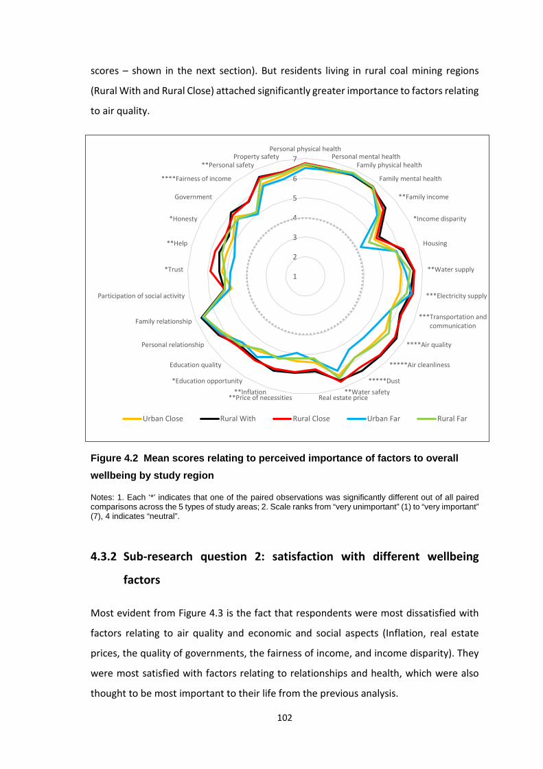
102

scores – shown in the next section). But residents living in rural coal mining regions

(Rural With and Rural Close) attached significantly greater importance to factors relating

to air quality.

Figure 4.2 Mean scores relating to perceived importance of factors to overall wellbeing by study region

Notes: 1. Each ‘*’ indicates that one of the paired observations was significantly different out of all paired comparisons across the 5 types of study areas; 2. Scale ranks from “very unimportant” (1) to “very important” (7), 4 indicates “neutral”.

4.3.2 Sub-research question 2: satisfaction with different wellbeing

factors

Most evident from Figure 4.3 is the fact that respondents were most dissatisfied with

factors relating to air quality and economic and social aspects (Inflation, real estate

prices, the quality of governments, the fairness of income, and income disparity). They

were most satisfied with factors relating to relationships and health, which were also

thought to be most important to their life from the previous analysis.

1

2

3

4

5

6

7Personal physical health

Personal mental healthFamily physical health

Family mental health

**Family income

*Income disparity

Housing

**Water supply

***Electricity supply

***Transportation andcommunication

****Air quality

*****Air cleanliness

*****Dust**Water safety

Real estate price**Price of necessities**Inflation

*Education opportunity

Education quality

Personal relationship

Family relationship

Participation of social activity

*Trust

**Help

*Honesty

Government

****Fairness of income

**Personal safetyProperty safety

Urban Close Rural With Rural Close Urban Far Rural Far

103

Figure 4.3 Mean scores relating to satisfaction with wellbeing factors displayed from most dissatisfied to most satisfied Notes: 1. Scale ranks from “very dissatisfied” (1) to “very satisfied” (7), 4 indicates “neutral”; 2. Red colour indicates negative impacts, while blue colour indicates positive impacts.

Visually, it is evident from Figure 4.4 that people from all areas were quite satisfied with

their health and their relationships (mean scores were generally around 6 without any

significant difference between study regions). Responses to questions about satisfaction

with family income were also similar across regions. The mean score relating to income

is approximately 4 (without a significant difference between coal mining and non-coal

mining areas), indicating that people in coal mining areas, were not more satisfied with

their family income than those from non-coal mining areas. Rural residents living with

and close to coal mining were less satisfied with income disparity than rural residents

living far from coal mining.

1 2 3 4 5 6 7

Family relationshipPersonal relationshipFamily mental health

Family physical healthElectricity supply

Personal mental healthPersonal physical health

Transportation and communicationHelp

Water supplyPersonal safety

TrustHousingHonesty

Participation of social activityEducation quality

Family incomeProperty safety

Water safetyEducation opportunity

Price of necessitiesIncome disparity

Fairness of incomeGovernment

Air qualityAir cleanliness

Real estate priceDust

Inflation

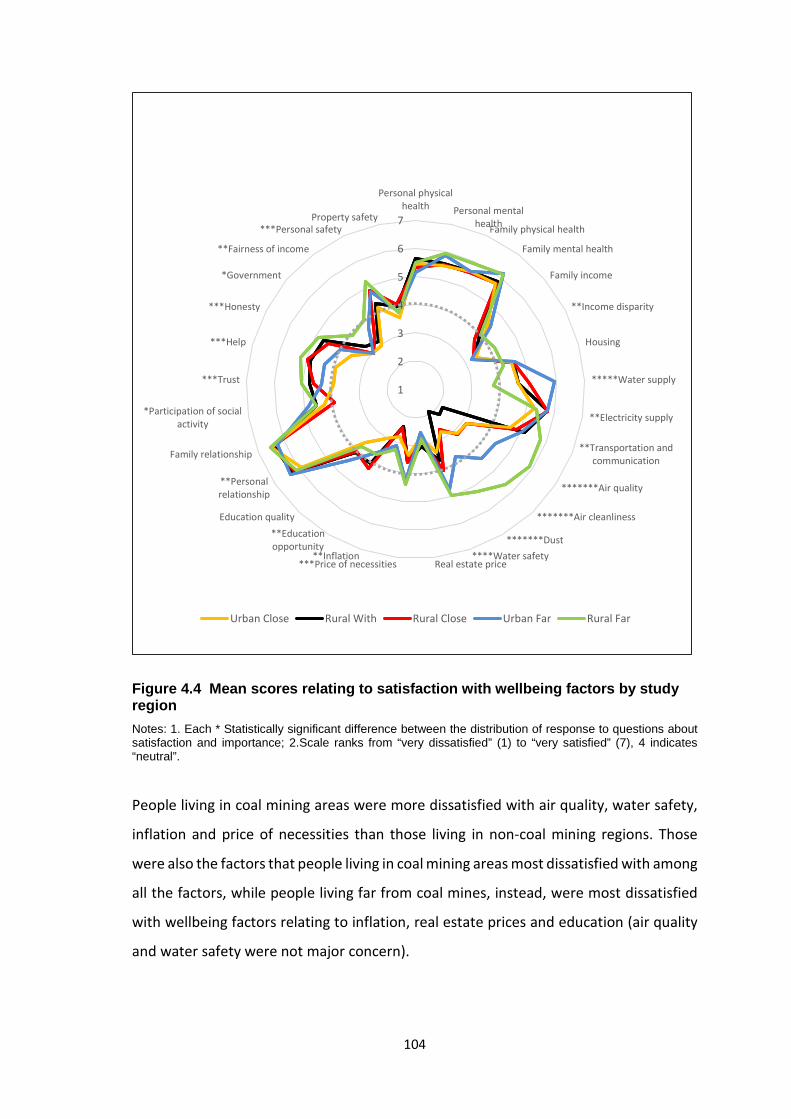
104

Figure 4.4 Mean scores relating to satisfaction with wellbeing factors by study region Notes: 1. Each * Statistically significant difference between the distribution of response to questions about satisfaction and importance; 2.Scale ranks from “very dissatisfied” (1) to “very satisfied” (7), 4 indicates “neutral”.

People living in coal mining areas were more dissatisfied with air quality, water safety,

inflation and price of necessities than those living in non-coal mining regions. Those

were also the factors that people living in coal mining areas most dissatisfied with among

all the factors, while people living far from coal mines, instead, were most dissatisfied

with wellbeing factors relating to inflation, real estate prices and education (air quality

and water safety were not major concern).

1

2

3

4

5

6

7

Personal physicalhealth Personal mental

healthFamily physical health


Family income

**Income disparity

Housing

*****Water supply

**Electricity supply

**Transportation andcommunication

*******Air quality

*******Air cleanliness

*******Dust****Water safety

Real estate price***Price of necessities**Inflation

**Educationopportunity

Education quality

**Personalrelationship

Family relationship

*Participation of socialactivity

***Trust

***Help

***Honesty

*Government

**Fairness of income

***Personal safetyProperty safety


105

There were few wellbeing factors that people living in coal mining area were more

satisfied with than their ‘non-coal mining’ counterparts. Most interesting of all, perhaps,

was the fact that people living in rural areas far from coal mining seem more satisfied

with more wellbeing factors relating to air quality, water safety, the price of necessities,

the quality of government and fairness of income and social capital (trust, help and

honesty) than those living in any other region.

Distance from coal mining seems to be a decisive factor which affects the satisfaction

with air quality, as people living in places far from coal mining, irrespective of whether

they were in rural or urban areas, were more satisfied with air quality than those living

in the places with or close to coal mining.

Responses to the question about water supply are a little more difficult to interpret,

because answers may indicate (dis)satisfaction with either infrastructure or with the

environment. Underground water is the main source of water supply in the case-study

area, and not all regions have piped water in all houses.

• People living in urban areas far from coal mining were most happy with water

supply, as ‘Urban Far’ represents the best situation – little damage to

underground water resources from coal mining, and better water infrastructure,

than in other areas.

• In rural regions far from coal mines (the least developed region among all the

groups), satisfaction with water supply was much lower than in other regions.

• The ‘moderate’ satisfaction scores in places that were adjacent to or close to

coal mines, may reflect the fact that although underground water supplies may

have been damaged by coal mining, the mining activity was likely to have

increased local government/council incomes enough to upgrade water supply

facilities, thus the improved infrastructure may be partially compensating for

real or perceived damage to underground water supplies. It became evident,

while undertaking fieldwork, that in some villages adjacent to coal mines,

residents relied on the coal company for water infrastructure.

106

Water safety is mainly associated with the existence of coal mining. People in the non-

coal mining area were more satisfied with water safety than those in the coal mining

area. In the coal mining areas, those living in the rural areas with coal mining were least

satisfied with water safety than those living in the urban and rural area close to coal

mining.

Those living in rural areas felt better able to trust, help and be honest with each other

than those in urban areas. This urban-rural ‘divide’ with respect to social capital is likely

due to more active social networks, civic participation and cohesion in rural areas

(Hofferth and Iceland, 1998; Ziersch et al., 2009).

4.3.3 Sub-research question 3: perceptions of the impacts of coal mining

on wellbeing factors

Generally, people’s perception of the impacts of coal mining on most factors were

negative, especially factors that relate to the natural environment and health (see Figure

4.5) 11. The only factor thought to be positively impacted by coal mining was family

income. Electricity supply, participation in social activities, relationships were thought

to have no obvious relationship with coal mining.

11 In the places far from coal mining, residents generally believed their daily lives were not related to coal

mining, thus they were not affected by coal mining. Therefore, instead of asking how they thought coal

mining affected them in their real life, they were asked the impacts they would expect if they had coal

mining in their places.

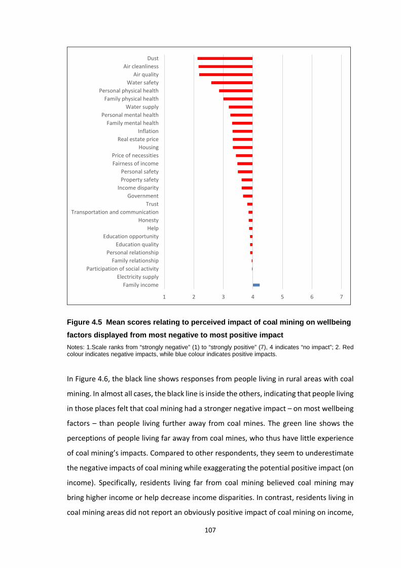
107

Figure 4.5 Mean scores relating to perceived impact of coal mining on wellbeing factors displayed from most negative to most positive impact Notes: 1.Scale ranks from “strongly negative” (1) to “strongly positive” (7), 4 indicates “no impact”; 2. Red colour indicates negative impacts, while blue colour indicates positive impacts.

In Figure 4.6, the black line shows responses from people living in rural areas with coal

mining. In almost all cases, the black line is inside the others, indicating that people living

in those places felt that coal mining had a stronger negative impact – on most wellbeing

factors – than people living further away from coal mines. The green line shows the

perceptions of people living far away from coal mines, who thus have little experience

of coal mining’s impacts. Compared to other respondents, they seem to underestimate

the negative impacts of coal mining while exaggerating the potential positive impact (on

income). Specifically, residents living far from coal mining believed coal mining may

bring higher income or help decrease income disparities. In contrast, residents living in

coal mining areas did not report an obviously positive impact of coal mining on income,

1 2 3 4 5 6 7

Family incomeElectricity supply

Participation of social activityFamily relationship

Personal relationshipEducation quality

Education opportunityHelp

HonestyTransportation and communication

TrustGovernment

Income disparityProperty safetyPersonal safety

Fairness of incomePrice of necessities

HousingReal estate price

InflationFamily mental health

Personal mental healthWater supply

Family physical healthPersonal physical health

Water safetyAir quality

Air cleanlinessDust

108

but instead reported negative impacts on income disparity. This is also consistent with

the observation from 4.3.2: people in coal mining areas were not more satisfied with

their family income or with income disparity than those from non-coal mining areas.

Also, different from residents living in coal mining areas, those living far from coal mining

do not seem to think that coal mining would negatively impact the quality of

government and/or fairness of income (in contrast to those who live with or near

mining).

Figure 4.6 Mean scores relating to perceived impact of coal mining on wellbeing factors by study region

Notes: 1.Each ‘*’ indicates that one of the paired observations was significantly different out of all paired

comparisons across the 5 types of study areas; 2. Scale ranks from “strongly negative” (1) to “strongly

positive” (7), 4 indicates “no impact”.

1

2

3

4

5

6

7***Personal physical health

***Personal mental health***Family physical health

**Family mental health

****Family income

****Income disparity

***Housing

*Water supply

Electricity supply

*Transportation andcommunication

***Air quality

***Air cleanliness

****DustWater safety

Real estate pricePrice of necessitiesInflation

***Education opportunity

****Education quality

*Personal relationship

Family relationship

**Participation of social activity

**Trust

**Help

Honesty

*****Government

***Fairness of income

***Personal safety**Property safety


109

Despite the optimism from people living far away from coal mines, in coal mining areas,

respondents did not identify any obviously positive impacts (see Figure 4.6). Factors

which related to the environment (e.g. air quality, water safety, access to water), the

economy (e.g. inflation and real estate price) and health (physical and mental health)

were all thought to be negatively affected by coal mining in all areas (mean score below

4). As illustrated below, coal mining had potential impacts on people’s lives through its

impacts on the natural environment – e.g. on water, hence the need to travel long

distances for water (see Figure 4.7) and a visual impact (as per the white dog, turned

black) (see Figure 4.8). This is also consistent with the message derived from Figure 4.4

– those living adjacent to coal mines were generally less satisfied with the wellbeing

factors that were generally thought to be negatively affected by coal mining.

Figure 4.7 Travelling long distance to get water

Note: Due to a period of coal mining, the underground water was damaged. Village folk have to travel far

to get water for daily use.

Source: Taken by the investigator in a village with coal mining on 22th August 2013

110

Figure 4.8 A little “white dog” in a village with coal mining

Note: This white street dog turned to black due

to exposure to coal dust.

Source: Taken by the investigator in a village

with coal mining on 21th September 2013

Figure 4.9 A little dog in a city close to coal mining

Note: This was a clean street dog with normal colour as the coal dust was not very heavy.

Source: Taken by the investigator in a city close to coal mining on 28th September 2013

4.3.4 Research question 4: the relationship between satisfaction and

importance

Figure 4.10 depicts people’s (mean) satisfaction with each of the 29 factors, together

with the importance they attach to each. The satisfaction score is significantly lower

than importance scores for all wellbeing factors except personal relationships. This

result is similar to that of Larson et al. (2014), although the wellbeing factors used in that

study were different due to a different purpose of their research. Generally,

relationships, including family relationships and personal relationships, were very

important, and people were satisfied with their own relationships. By contrast, air

quality was deemed important, but people were generally very dissatisfied with it. Other

factors that were important but which people were dissatisfied with included fairness

of income, the quality of government, income disparity, inflation and real estate prices.

111

Figure 4.10 Mean scores relating to satisfaction with and importance of wellbeing factors

Notes: 1.Wellbeing factors ranks by the scores of importance; 2. ‘*’ indicates statistically significant difference between the distribution of response to questions about satisfaction and importance; 2. Scale ranks from “very unimportant /dissatisfied” (1) to “very important/satisfied” (7), 4 indicates “neutral”.

Figure 4.11 shows the mean importance score associated with each factor, plotted

against the mean Dis-Satisfaction score. The majority of the wellbeing factors in the

graph appear to be arranged along a negatively sloping curve (R2=0.216). Those

receiving high dissatisfaction scores and importance (relating to the natural

environmental (air quality, dust, air cleanliness and water safety) and the economy

(inflation and real estate prices)) are in the upper right quadrant of the graph, those

receiving low dissatisfaction scores (health) and high importance scores are in the lower

right quadrant. Generally, there are no outliers (i.e. no factors that receive very high/low

dissatisfaction scores but very low importance scores). This relationship is generally

consistent with the argument of Friedlander (1965) and Trauer and Mackinnon (2001),

but the linear relationship was not very strong – similar to the findings of (Chen and Lin,

2014) – which suggested a need for more detailed investigations of the relationship

between those variables.

1

2

3

4

5

6

7*Family physical health

*Personal physical health*Family mental health

*Family relationship

*Personal mental health

*Water safety

*Personal safety

*Water supply

*Property safety

*Air quality

*Electricity supply

*Air cleanliness

*DustPersonal relationship

*Family income*Transportation and communication*Housing

*Education quality

*Government

*Inflation


*Price of necessities

*Real estate price

*Fairness of income

*Help

*Trust

*Honesty

*Participation of social activity*Income disparity

Satisfaction Importance

112

Figure 4.11 The relationship between mean scores relating to dissatisfaction and importance Notes: Scale of satisfaction ranks from “very satisfied” (1) to “dissatisfied” (7), 4 indicates ‘neutral’; Scale of

importance ranks from “slightly important” (3) to “very important” (7), 4 indicates “neutral”. No factors have

score of ‘importance’ below 3.

Table 4.1 presents the Indices of Dis-Satisfaction (IDS), for each factor, by case-study

area. The indices are remarkably different between coal mining areas (Urban close, Rural

With and Rural Close) and non-coal mining areas (Urban Far and Rural Far). In coal

mining areas, wellbeing factors relating to the natural environment (especially dust in

the air) and the economy (inflation and the price of real estate prices) have the highest

indices, while in non-coal mining areas, environment indicators have relatively low

indices; instead, real estate prices, inflation, property safety and education system

emerge as policy priorities (with the higher indices). Real estate prices and inflation are

common issues in all the places, with a slightly higher values of IDS in coal mining areas

– indicating a bigger magnitude of problems in coal mining areas.

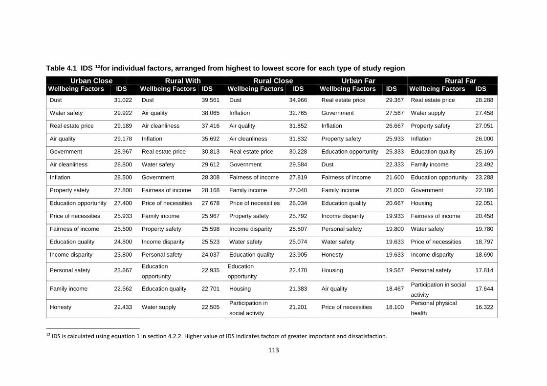
113

Table 4.1 IDS 12for individual factors, arranged from highest to lowest score for each type of study region Urban Close Rural With Rural Close Urban Far Rural Far

Wellbeing Factors IDS Wellbeing Factors IDS Wellbeing Factors IDS Wellbeing Factors IDS Wellbeing Factors IDS Dust 31.022 Dust 39.561 Dust 34.966 Real estate price 29.367 Real estate price 28.288

Water safety 29.922 Air quality 38.065 Inflation 32.765 Government 27.567 Water supply 27.458

Real estate price 29.189 Air cleanliness 37.416 Air quality 31.852 Inflation 26.667 Property safety 27.051

Air quality 29.178 Inflation 35.692 Air cleanliness 31.832 Property safety 25.933 Inflation 26.000

Government 28.967 Real estate price 30.813 Real estate price 30.228 Education opportunity 25.333 Education quality 25.169

Air cleanliness 28.800 Water safety 29.612 Government 29.584 Dust 22.333 Family income 23.492

Inflation 28.500 Government 28.308 Fairness of income 27.819 Fairness of income 21.600 Education opportunity 23.288

Property safety 27.800 Fairness of income 28.168 Family income 27.040 Family income 21.000 Government 22.186

Education opportunity 27.400 Price of necessities 27.678 Price of necessities 26.034 Education quality 20.667 Housing 22.051

Price of necessities 25.933 Family income 25.967 Property safety 25.792 Income disparity 19.933 Fairness of income 20.458

Fairness of income 25.500 Property safety 25.598 Income disparity 25.507 Personal safety 19.800 Water safety 19.780

Education quality 24.800 Income disparity 25.523 Water safety 25.074 Water safety 19.633 Price of necessities 18.797

Income disparity 23.800 Personal safety 24.037 Education quality 23.905 Honesty 19.633 Income disparity 18.690

Personal safety 23.667 Education

opportunity 22.935 Education

opportunity 22.470 Housing 19.567 Personal safety 17.814

Family income 22.562 Education quality 22.701 Housing 21.383 Air quality 18.467 Participation in social

activity 17.644

Honesty 22.433 Water supply 22.505 Participation in

social activity 21.201 Price of necessities 18.100

Personal physical

health 16.322

12 IDS is calculated using equation 1 in section 4.2.2. Higher value of IDS indicates factors of greater important and dissatisfaction.

114

Urban Close Rural With Rural Close Urban Far Rural Far Wellbeing Factors IDS Wellbeing Factors IDS Wellbeing Factors IDS Wellbeing Factors IDS Wellbeing Factors IDS

Trust 20.989 Housing 20.780 Trust 20.309 Personal physical

health 17.900 Electricity supply 16.322

Help 20.733 Honesty 18.121 Transportation &

communication 20.242 Air cleanliness 17.700 Honesty 16.322

Housing 20.522 Participation in

social activity 17.958 Personal safety 20.121 Help 17.033 Dust 15.610

Water supply 20.111 Transportation &

communication 17.621 Honesty 19.255 Trust 16.700 Trust 14.119

Transportation &

communication 19.189 Trust 17.033 Water supply 18.289

Transportation &

communication 16.367

Family physical

health 14.069

Participation in social

activity 17.178 Help 16.879 Personal physical

health 18.262 Family physical

health 16.233 Help 13.508

Personal physical

health 16.811 Personal physical

health 15.869 Help 17.732 Participation in social

activity 14.900 Personal mental

health 13.458

Personal mental

health 15.878

Personal mental

health 15.682

Personal mental

health 16.678 Electricity supply 14.700 Air cleanliness 13.458

Electricity supply 15.789 Family physical

health 15.603

Family physical

health 16.436

Personal mental

health 14.067 Air quality 12.678

Family physical

health 15.611 Electricity supply 14.631 Family mental

health 15.523 Water supply 12.400 Transportation &

communication 12.475

Family mental health 14.767 Family mental

health 14.472 Electricity supply 14.765 Family mental health 12.200 Family mental health 12.328

Personal relationship 12.267 Personal

relationship 10.664

Personal

relationship 11.195 Family relationship 11.600 Personal relationship 10.610

Family relationship 9.722 Family relationship 10.402 Family relationship 10.322 Personal relationship 10.000 Family relationship 9.610

115

4.3.5 Research question 5: the relationship between satisfaction level

and the impact of coal mining

Figure 4.12 depicts people’s (mean) satisfaction with each of the 29 factors, together

with the (mean) score relating to the perceived impacts of coal mining on each factor.

In coal mining areas, the factors that people were most dissatisfied with included those

relating to: air quality (dust, air quality, and air cleanliness), inflation, the price of real

estate and necessities, the quality of government, the fairness of income, income

disparity and water safety. These factors (especially those relating to the natural

environment) were also the factors which respondents felt that coal mining generally

had negative impact on.

Figure 4.12 Mean scores relating to satisfaction with and perceived impact of coal mining on wellbeing factors Notes: 1. Wellbeing factors ranks by the scores of satisfaction; 2. ‘*’ indicates statistically significant difference between the distribution of response to questions about satisfaction and importance; 3. Scale ranks from “very dissatisfied/negative impacts” (1) to “very satisfied/positive impacts” (7), 4 indicates “neutral/no impacts”. 4. Only samples from coal mining areas (Urban Close, Rural With, Rural Close) are included in this graph.

1

2

3

4

5

6

7*Family relationship

Personal relationship*Family mental health

*Family physical health

*Electricity supply

*Personal mental health

*Personal physical health

*Transportation and communication

*Help

*Water supply

*Personal safety

*Trust

*House*Honesty

*Participation of social activity*Education quality*Family income

*Property safety

*Water safety


*Price of necessities

*Income disparity

*Fairness of income

*Government

*Air quality

*Air cleanliness

*Real estate price

*Dust*Inflation

Satisfaction Impact of coal mining

116

As discussed in section 4.3.2, there were few wellbeing factors that people living in coal

mining area were more satisfied with than their ‘non-coalmining’ counterparts (see

Figure 4.4). The factors related to the natural environment (air quality and water safety),

which were believed to be most negatively affected by coal mining (see section 4.3.3),

were also those where the gap between satisfaction scores in coal mining and non-coal

mining areas was greatest (see Figure 4.4).

Coal mining was also perceived to have negative impacts on others factors, such as

health, but people seemed quite satisfied with these factors, suggesting that they might

not be as high a policy priority as other factors (also, fixing environmental issues, could

help mitigate at least some health issues).

To further explore the relationship between satisfaction and perceived impacts of coal

mining, the mean dissatisfaction of each factor was plotted against its mean negative

impact score for the coal mining areas (Figure 4.13). Only coal mining areas were

included in this analysis. In these areas, there were a number of factors (mainly

environment factors) appearing in the upper right quadrant of the graphs, indicating

both high levels of dissatisfaction, and ‘blame’ being attributed to coal mining.

117

Figure 4.13 The relationship between mean scores relating to dissatisfaction and perceived impact of coal mining Notes: Scale of satisfaction ranks from “very satisfied” (1) to “dissatisfied” (7), 4 indicates ‘neutral’; Scale of

negative impact ranks from “slightly negative” (3) to “strongly positive” (7); 4 indicates “no impact”. No factors

have score of ‘negative impact’ below 3.

Table 4.2 presents the IDSNI scores associated with each factor, for each type of case-

study area. Dust, air quality, air cleanliness, water safety, real estate prices and inflation

were clearly identified as factors with the highest levels of dissatisfaction, on which coal

mining is perceived as having a strong negative impact. These factors emerge at the top

5 of IDSNI ranking and are very consistent across all the coal mining areas.

118

Table 4.2 IDSNI13 for individual factors, arranged from highest to lowest score for 3 types of study region

Urban Close Rural With Rural Close Wellbeing Factor IDSNI Wellbeing Factor IDSNI Wellbeing Factor IDSNI

Dust 31.60 Dust 39.27 Dust 30.01

Air quality 29.07 Air quality 37.57 Air cleanliness 27.41

Air cleanliness 28.99 Air cleanliness 37.20 Air quality 27.26

Real estate price 27.21 Inflation 27.10 Inflation 26.19

Water safety 26.88 Water safety 25.49 Real estate price 23.64

Inflation 24.72 Real estate price 24.20 Water safety 22.09

Fairness of income 23.22 Fairness of income 23.14 Government 21.30

Price of necessities 22.30 Government 21.91 Fairness of income 20.79

Government 21.62 Income disparity 21.54 Price of necessities 20.43

Income disparity 21.31 Price of necessities 20.82 Income disparity 20.34

Education opportunity 20.80 Personal safety 18.80 Property safety 16.54

Property safety 19.17 Property safety 18.66 Family income 16.41

Education quality 18.79 Water supply 18.19 Participation in social activity 16.40

Honesty 18.04 Housing 17.60 Education quality 15.97

Water supply 17.30 Education opportunity 16.78 Housing 15.27

Trust 16.79 Education quality 16.49 Education opportunity 15.11

Help 16.49 Family income 15.96 Water supply 14.43

Personal safety 16.16 Participation in social activity 14.35 Honesty 14.22

Housing 15.27 Honesty 14.20 Trust 13.86 Transportation and communication 14.75 Trust 13.86 Personal safety 13.84

Participation in social activity 14.74 Help 13.15 Transportation and

communication 13.55

Personal physical health 13.35 Personal physical health 13.07 Personal physical health 13.05

Family income 13.13 Family physical health 12.86 Help 12.37

Family physical health 11.98 Personal mental health 12.83 Family physical health 11.88

Personal mental health 11.33 Transportation and communication 12.19 Personal mental health 11.51

Electricity supply 11.09 Family mental health 11.14 Family mental health 10.59

Family mental health 10.45 Electricity supply 9.17 Electricity supply 9.14

Personal relationship 8.60 Personal relationship 7.34 Personal relationship 7.24

Family relationship 5.94 Family relationship 6.62 Family relationship 6.17

13 IDSNI is calculated using equation 2 in section 4.2.3. Higher value of IDSNI indicate factors with which people are more dissatisfied and coal mining has stronger negative impacts on.

119


Key findings are summarised in Table 4.3 and discussed in more detail below.

Table 4.3 Summary of findings

Urban Close Rural With Rural With Urban Far Rural Far Common issues

Specific to mining

Importance

Family physical health

Personal physical health




Health and relationship

Mean importance scores do not vary dramatically across different types of case-study regions, except factors relating to air quality.

Family relationship



Family mental health Personal physical health


Family relationship


Family relationship Family mental health



Water safety Personal physical health

Personal mental health


Air quality Personal mental health


Family relationship

Perceived impacts

Dust Dust Dust Dust Air quality

Dust, air cleanliness, air quality, water safety,

Although the top 5 perceived impacts of coal mining were similar across regions, perceived impacts on income and income disparity vary between coal mining and non-coal mining regions.

Air cleanliness Air cleanliness Air cleanliness Air cleanliness Air cleanliness

Air quality Air quality Air quality Air quality Dust

Water safety Water safety Water safety Water safety Water safety

Real estate price Personal physical health




Real estate price Dust Inflation Real estate price Real estate price

120

Urban Close Rural With Rural With Urban Far Rural Far Common issues

Specific to mining

Dis–Satisfaction

Dust Air quality Dust Government Inflation Dust, air cleanliness, air quality, water safety, real estate price, inflation

The most dissatisfying factors in coal mining areas related to the environment and the economy, while most dissatisfying factors in non-coal mining areas only related to the economy.

Inflation Air cleanliness Real estate price Inflation Education opportunity

Fairness Inflation Government Income disparity Education quality

Government Real estate price Air quality Education opportunity Water supply

IDS

Dust Dust Dust Real estate price Real estate price

Real estate price, inflation

In coal mining areas, both environmental and economic issues emerge on the top of IDS list, but the environment is not a concern in non-coal mining areas.

Water safety Air quality Inflation Government Water supply

Real estate price Air cleanliness Air quality Inflation Property safety

Air quality Inflation Air cleanliness Property safety Inflation

Government Real estate price Real estate price Education opportunity Education quality

IDSNI

Dust Dust Dust

None

In coal mining areas, both environmental and economic issues emerge on the top of IDSNI list.

Air quality Air quality Air cleanliness

Air cleanliness Air cleanliness Air quality

Real estate price Inflation Inflation

Water safety Water safety Real estate price

121

In this case-study region, factors associated with health and relationship were deemed

– by the entire sample, and by each sub-sample – to be the most important contributors

to wellbeing. For most factors, mean importance scores do not vary dramatically across

different case-study regions, except factors relating to air quality. Health and

relationship were also the factors with which people in each sub-sample were most

satisfied. People in coal mining areas were most dissatisfied with factors relating to air

quality and the economy, while people in non-coal mining areas were most dissatisfied

with factors only relating to the economy. People expressed most concern about the

impacts of mining on the environment (air quality and water safety) and health, which

is consistent across all the case-study regions. Compared to people living in coal mining

regions, people living in non-coal mining regions seem to underestimate the negative

impacts of coal mining while exaggerating the potential positive impacts.

Respondents from rural areas with coal mining recorded the strongest perceptions

about the negative impacts of mining on most wellbeing factors, and were most

dissatisfied with factors relating to the environment. Those with little exposure to coal

mining (i.e. respondents living far away from coal mining) expected that coal mining

would bring (comparatively) less severe negative impacts than those who lived with or

near coal, and expected stronger positive impacts on their household income and on

income disparities.

No similar study could be found in a mining context with which to compare these results,

however, similar observations have been found in a tourism context. Termed the

“Irridex model”, this theory “postulates that resident's attitudes towards tourism are

euphoric in the early stages, progressing to apathy, irritation and, eventually,

antagonism” (Diedrich and García-Buades, 2009, p. 519). Observations from this study

suggest that the Irridex model might also apply in a mining context, in that those with

little experience of the industry seemed to underestimate its potential negative impacts,

and overestimate its positive impacts. This is particularly so in rural areas, where poverty

is a significant problem, and the prospect for higher incomes from mining is very

attractive. Some village folks said: “We will be lucky if we have coal mining in our village.

Life will be better because we could get money from that.”

122

People in rural areas had stronger views about the potential impacts of coal mining than

those in urban areas. The economy in rural areas is less developed and less diverse than

that in urban areas, and the available options for livelihoods is also very limited (Kanbur

and Zhang, 2005; Sicular et al., 2007). This may at least partially explain why rural

residents who have no experience of mining hold relatively positive attitudes towards it,

given the potential for coal mining to diversify their livelihoods. That said, rural residents

are also likely to be dramatically impacted by coal mining once they have it (Rural With).

Residents from urban areas with more diverse industries and more options for

livelihoods, had more balanced views on mining – they were neither so strongly exposed

to coal mining (Urban Close), nor longed for the benefits from coal mining (Urban far)

as their rural counterparts. The urban sample from which these insights have been

drawn is, however, relatively small: future studies are needed to explore the

dependence on mining industry in terms of the differences between urban and rural

areas.

Importantly, this analysis relies on aggregated data and thus describes the ‘average’

situation in each type of study region. This does not mean that each village (or each

individual within each village) is in the same situation, given the diversity of villages and

individuals included in this study. While environmental damage was a common concern

across all villages with or close to coal mining, a diverse range of other issues impacted

different villages in different ways. As discussed below, this is likely to have led people

to have quite different attitudes towards coal mining – even if living within the same

village or same ‘type’ of case-study area.

• The ownership and location of coal mines

After the coal mine consolidation program (which was advanced by the government

from 2009 onwards), more than half of the coal mines came under the control of

government (Zhou, 2011), and most illegal coal mines were closed. But there are still a

small number of ‘illegal’ coal mines scattered around Shanxi province, and these often

generate conflicts between the coal mine operators, the local governments and host

communities. In one village, an illegal coal mine was located almost in the backyard of

several houses, but was only operated at night to avoid trouble. There were continuous

123

conflicts between the owners of this coal mine and village folk, as evidenced by the

following comments made by respondents when collecting data:

“The head of our village has shares in the coal mine, they are on one side against

us.”

“A lady was even badly injured in the conflict. Since then, nobody tried to fight

with the owner of the coal mine and the local government”.

People living in this village generally had strong negative attitudes towards coal mining.

• The distance of the individual from coal mines or coal transportation

In the same village referred to above, a lady living beside the road, could never go to

sleep because heavy trucks passed by her front door almost 24 hours a day. A special

road was built for the transport of coal, but the truck drivers were reluctant to use it –

the road through the village was shorter and more direct. In another village with coal

mining, explosives were regularly used, breaking windows and causing cracks to the

houses nearby. These respondents generally had more strong negative attitudes

towards coal mining than others in the same village who lived further away from the

road or the area were explosives were set.

Figure 4.14 Heavy truck carrying coal through the middle of a village Source: Taken by the investigator in a village with coal mining on 22th August 2013

124

• Association with the coal mining industry

People living in places with coal mining tended to have extreme attitudes towards coal

mining; these varied according to whether they (or someone else in their immediate

family) were working in the coal mine or were dependent upon some other industry (e.g.

agriculture) for their livelihood.

In one of the villages with a coal mine, people’s attitudes towards coal mining were

generally positive – perhaps at least partially because the coal company had, as policy,

the goal of hiring at least 1 person from each household. Anecdotal evidence suggests

that this policy arose because the chairman of the coal company is from that village.

When a woman was asked about the impacts of coal mining, she was hesitant to express

openly what she actually thought. “I don’t want to say anything bad about coal mining,

because my whole family is counting on it. If coal mines are closed here, my husband will

lose his job, and we cannot make a living”. Notably, this situation is rare – it was the only

village visited by investigators that seemed to have a generally positive outlook on

mining.

In contrast, in another village with coal mining where people did not obviously benefit

from coal mining, the attitudes towards to coal mining were uniformly negative. A family

reliant on agriculture obviously resented coal mining: “coal mining brings me nothing

but misery. A lot of my sheep died after they ate the grass covered by coal dust. Some of

them fell down into a crack [in the ground] caused by coal mining, now I don’t have many

sheep left”.

Compared to those who lived in villages that had a coal mine within its boundaries, the

attitudes of people living in villages that were a little more removed from the mine

(formally classified as being ‘close to’ coal mining) were much more neutral. They were,

however, acutely aware of the potential negative impacts of coal mining, and may have

even directly experienced some. One man said:

“I felt lucky that we don’t have coal mines in our village, so I still have my

farmland, I have been doing odd jobs with an unsatisfying income in the city, but

my farmland makes me feel secure. Rumour has it that coal has been found

125

underground in my village. I would definitely be the first person opposed to coal

mining here, because ordinary people like me could not benefit from coal mining,

only those officers or rich people can. If they start mining here, the only

consequences will be that we will lose farm land and suffer from all the

environmental damage from coal mining. Even now, it already has impacts on us.

In the farmland beside the special road for coal transportation, the corncobs are

black inside. But there was no compensation for that.” (To reduce the dust from

coal transportation, it is required by law that all the trucks carrying coal should

be covered by a special cloth. However, it was said that 99% of these trucks are

not covered).

The diversity of perspectives clearly indicates that having a single “standard” policy

towards all mining in the developing world or even a single “standard” policy towards

all mining across all regions within a single country may be undesirable. The data reveal

several common issues associated with coal mining (generally negative environmental

impacts, and few positive economic impacts), but there is diversity at a village level.

Having a solid understanding of unique situations and of the reason behind diverse

perspectives could help inform development of regional specific policies better able to

improve the wellbeing of residents in coal mining areas.

There is also much diversity at an individual level. In particular, one expects that the

importance which individuals attach to wellbeing factors, people’s satisfaction with

various wellbeing factors and their perceptions about the impacts of coal mining on

those factors will depend upon a host of other factors, not the least of which relate to

‘personality’ and to the sociodemographic characteristics and economic status of

individuals. But these are all subjective indicators of wellbeing; as discussed in section

2.3.1.2, objective indicators, traditionally used by governments, can also be used to

assess wellbeing. Is the message from subjective wellbeing mirrored by objective

indicators? This question will be explored in the following chapter.

126


Using subjective indicators, this chapter provides useful information to help assess the

likely impacts of mining and identify regional policy priorities.

All indicators suggest that environmental problems should be the policy priority in the

coal mining areas. In particular, both the composed Index of Dis-Satisfaction (IDS) and

Index of Dis-Satisfaction and Negative impacts (IDSNI) indicate that both environmental

issues (air quality and water safety) and economic issues (the inflation rate and the price

of real estate prices) were of high priority in coal mining areas, and environmental issues

were paramount. However, IDS indicates that priority lists differed between coal and

non-coal mining areas. In non-coal mining areas, factors relating to the environment

were not a ‘priority’, instead, economic issues and social issues (the quality of

government and education) were of most concern.


This chapters clearly demonstrated a technique for identifying different policy priorities

in mining and non-mining areas. The technique is largely transferrable to other contexts

– to consider the impacts of an industry, or a project and to generate straightforward

‘action-lists’ to infer public policy priorities.

If seeking to replicate this type of study in another context, one could develop a list of

potential wellbeing factors that are likely to be affected by a particular project, and

information about those factors could be collected from different areas (e.g. those

which have been exposed to, or have lived with similar projects, and those where the

project is likely to be implemented) to learn more about its likely impact. This would

best be done by a combination of expert group and community qualitative research,

such as focus groups to determine consensus on factors. Follow-up studies could also

be implemented at regular intervals after project start, to gauge actual impact (and to

compare actual with projected impact for further information).

127

Thesis outline

128

5. CHAPTER 5 EXPLORING THE RELATIONSHIP BETWEEN

OBJECTIVE AND SUBJECTIVE INDICATORS OF WELLBEING

Chapter outline

5.1 Introduction


5.3 Results

5.3.1 The relationship between objective and subjective indicators relating to family income

5.3.2 The relationship between objective and subjective indicators relating to air quality

5.3.3 The relationship between objective and subjective indicators relating to housing

5.3.4 The relationship between objective and subjective indicators relating to education

5.4 Conclusion and Discussion



5.4.3 Implications for future studies

129

Synopsis

This chapter explores the relationship between 4 ‘pairs’ of objective and subjective

indicators relating to 4 different factors known to influence wellbeing. Data deficiencies

(mostly relating to objective indicators) precluded more comparisons. For each pair, I

explored the relationship between these two measures of wellbeing – using both

aggregated (regional) and individual data.

When using data at an aggregated regional level (across the 5 types of study region),

some of the ‘pairs’ of objective and subjective indicators conveyed very consistent

messages: high actual income was associated with high satisfaction with income, and

high concentration of PM10 was associated with low satisfaction with air quality.

However there was a divergence between other pairs of subjective and objective

indicators, such as those relating to housing and education, not conveying the same

message.

I also considered the relationship between objective and subjective indicators using

individual data. When doing so, each subjective indicator was regressed against its

‘paired’ objective indicator and sociodemographic variables known to influence

subjective assessments. In each case the regression was run using both the entire

dataset and then also sub-sets of data, relating to each type of study region. This analysis

confirmed the consistent message between the subjective and objective indicators

relating to income and air quality – although the relationship was mediated by

sociodemographic factors. Not all the objective indicators of housing are good

predictors of satisfaction with housing. The relationship between subjective and

objective indicators associated with education was, as for the aggregated data,

inconsistent. Thus, it is possible to conclude that objective and subjective indicators are

not always a substitute for each other; both are needed to gain a complete picture of

wellbeing in some cases.

130

5.1 Introduction

As noted before, coal is vitally important to both developed and developing economies.

But coal mining’s well documented harm to the natural environment and negative

effects on human mortality and morbidity has spurred a significant body of literature

that looks more broadly at the impacts of coal mining on various life domains. These

studies have, however, been largely limited to examining objective indicators of

wellbeing, with or without directly referring to the concept of wellbeing. Not only does

the current literature lack studies that investigate a broad range of SWB indicators, but

it is particularly impoverished when it comes to studies that compare or use both

subjective and objective indicators.

The previous chapter investigated various indicators of subjective wellbeing across 29

wellbeing factors. It considered the importance of each factor (to overall wellbeing),

people’s satisfaction with each factor, and their perceptions of the way in which coal

mining affects them. A complex picture emerged: people from areas with different

exposures to coal mining were differently satisfied with several wellbeing factors

(particularly those relating to the environment and the economy), but some differences

also seemed attributable to other factors (such as rural/urban contexts). Would the

message be similar if looking at objective indicators too? The main research question

addressed in this chapter is thus: Does information about the impacts of coal mining

derived from subjective assessments of wellbeing convey the same message about the

impacts of coal mining as ‘objective’ measures of wellbeing? This over-arching question

is answered with reference to the specific sub-questions below:

1) Do the objective indicators suggest that there are differences in wellbeing

between

a. Areas with different mining intensities;

b. Rural and urban areas.

2) Do objective and subjective indicators convey similar information?

a. Using aggregated data (Visually in the chart);

131

b. Using regressions at individual level to control for sociodemographic

factors.

The approaches used to analyse data are described in section 5.1. Section 5.2 presents

the methods used to address these questions, whilst section 5.3 presents results. This

chapter is closed by a discussion.


To examine the relationship between objective and subjective wellbeing indicators, one

first needs to identify ‘pairs’ of objective and subjective indicators which effectively align

(i.e. refer to the same wellbeing factor). As demonstrated in the last chapter, several

different types of subjective indicators associated with 29 different wellbeing factors

were collected in this study. It was much more difficult to obtain ‘objective’ measures

at small scale (e.g. village): few were available from central data-collection agencies, and

collecting objective measures for each wellbeing factors (e.g. crime or corruption rates

within each village) was well beyond the resources of this study. Nevertheless, it was

possible to obtain ‘objective’ indicators relating to income, air quality, housing and

education. The ‘pairs’ of subjective and objective indicators assessed in this chapter

thus include:

1. Actual family income and satisfaction with family income. Objective data

relating to actual family income were collected in the survey (see

Appendix A, Q49); Respondents were not asked to provide their exact

income; rather to indicate an income range. The midpoint of each range

was used as the estimate of family income. For the unbounded top

bracket ($120,000 Yuan), a fairly conservative mid point 125,000 was

assumed. This is applied onwards in this thesis. Subjective data about

family income are respondents’ self-reported satisfaction with their

family incomes (see Appendix A, Q10)

2. Actual air quality and satisfaction with air quality. Objective data relating

to air quality were concentrations of PM2.5 and PM10, measured during

132

the field visit and used as a crude proxy for environmental quality (OECD

2011). Both PM2.5 and PM10 have well documented adverse effects on

human health (Dockery et al. 1993). Only PM10 was used here, given the

close correlation in measures. Subjective data about air quality are

respondents’ self-reported satisfaction with the air quality in the places

they lived in (see appendix A, Q1914).

3. Actual housing conditions and satisfaction with housing. Objective data

relating to actual housing conditions were collected in the survey (see

Appendix A, Q51 and Q52). Respondents were asked to tell whether

he/she had a bathroom and toilet in his/her house, and how many rooms

were in the house (enabling me to calculate ‘rooms per person’). These

indicators were used as a crude proxy for housing conditions (OECD,

2011). Subjective data about housing are respondents’ self-reported

satisfaction with their own housing conditions (Q15).

4. Actual education levels and satisfaction with the current education

system (education quality and opportunity). Objective data relating to

education were collected in the survey (see Appendix A, Q46).

Respondents were asked to provide their education levels. The education

level then was converted to years of schooling to make the analysis more

straightforward. This is applied onwards in this thesis. Subjective data

about education are respondents’ self-reported satisfaction with the

education opportunity and quality in the places they lived in (Q27 and

Q28).

Having identified suitable ‘pairs’, data were divided according to 5 types of study region

( Urban Close, Rural With, Rural Close, Urban Far, Rural Far).

To answer research question 1 (part a and b), the mean value of each objective and

subjective indicator was calculated for each type of region. Non-parametric tests

14 Respondents were asked how satisfied they were with the air quality as a whole (appendix A, Q19), air cleanliness (Q20) and dust in the air (Q21). Only the air quality as a whole (Q19) was used here, as it might be more representative for the air quality, although the answer for the 3 questions were very consistent.

133

(Kruskal-Wallis) were then used to determine if the observed differences in objective

indicators across regions with different intensities of coal mining were statistically

significant, and if the difference between urban and rural areas was statistically

significant. Non-parametric tests (Kruskal-Wallis) were only done for objective

indicators; results of non-parametric tests relating to subjective wellbeing indicators

were presented in the previous chapter (see section 4.3.2) and also used for the analysis

here.

To answer research question 2a, the mean score of each objective and subjective

indicator (for each ‘pair’ of data) were plotted to visually determine if the indicators

were conveying similar types of information. The results of the non-parametric tests

(Kruskal-Wallis) conducted on both objective and subjective indicators were used to

further the analysis.

As discussed in section 2.3.2.6 and 3.4.1.2, sociodemographic factors such as marital

status (Ballas and Dorling, 2007; Brereton et al., 2008), age (Stutzer and Frey, 2008),

family size (Frijters and Van Praag, 1998), gender (Moro et al., 2008; Arifwidodo and

Perera, 2011) have all been shown to influence subjective assessments of wellbeing.

Furthermore, Lee and Marans (1980) noted that personal and social characteristic (such

as age, income, education etc.) affect the relationship between objective and subjective

indicators, they thus controlled for these factors in the regression when they examine

the relationship between objective and subjective indicators. Therefore, to further

explore the relationship between objective and subjective indicators of wellbeing (and

to answer research question 2b), each subjective indicator was thus regressed against

its ‘matching’ objective indicator and other sociodemographic (‘control’) variables

(derived from the literature review (see Table 3.6)), as detailed in Equation 3. Several

regressions were run for each pair of subjective and objective indicators: the first using

the entire sample, the others using sub-samples from each type of study region.

SATi = f (OWB, Agei, Female, NotPartneredi, NoOfChildreni, NoOfAdulti,

Schoolingi, EmploymentStatusi)

Where:

Equation 3

134

SATi – satisfaction score associated with a particular wellbeing factor, reported

by person i

OWBi – objective indicator associated with a particular wellbeing factor

NoOfChildreni – the total number of children living in the respondents house

NoOfAdulti – the total number of adults living in the respondents house

Agei – age of the respondents

Femalei – a dummy variable, set equal to 1 if person i was female (0 otherwise)

Notpartneredi – a dummy variable, set equal to 1 if person i had no partner (0 otherwise)

Schoolingi – maximum of years of schooling the respondent has

Employment

statusi

measured using a series of dummy variables, set equal to 1 if:

– retired

– jobless

– students

– self-employed

In these regressions, the dependent variable (the subjective indicator) was measured on

a 7-point Likert scale. As such, ordinary least squares regression (OLS) – which assumes

that the dependent variable is continuous – is not the theoretically correct regression

procedure. Usually, ordinal regression is more suitable. Both OLS and Ordinal regression

were thus used. The two different types of regression produced very similar results (in

terms of significance and relative magnitude of coefficients) 15 , which accords with

empirical findings from other researchers who have reported that choice of regression

technique has little or no impact on results (e.g. Frijters and Praag, 1998; Welsch, 2006;

Luechinger, 2009; MacKerron and Mourato, 2009; Ambrey and Fleming, 2011; Levinson,

2012). It is the OLS results which are reported on here, since they are more

straightforward and easier to interpret than results from ordinal regression (MacKerron

and Mourato, 2009).

15 See Appendix C for results of ordinal regressions examining the relationship between objective and subjective wellbeing indicators.

135

5.3 Results

5.3.1 The relationship between objective and subjective indicators

relating to family income

Figure 5.1 presents the plot of mean family income and satisfaction with income for each

type of study region. Visually, a higher level of family income is associated with a higher

level of satisfaction with income.

The non-parametric tests (Kruskal-Wallis test, pairwise comparisons) undertaken on

objective measures indicate that annual family income in urban areas is significantly

higher than in rural areas (p = 0.000), irrespective of their proximity to coal mines.

Although there is no statistically significant difference in satisfaction with income across

the 5 regions (see the result of Kruskal-Wallis test in Figure 4.4), Figure 5.1 clearly

demonstrates that, people living in rural areas were generally dissatisfied with their

family income (mean values were below 4), while people living in urban areas were

generally satisfied with their family income (mean values were above 4). As such, both

the objective and subjective measures relating to income convey a consistent message:

higher family income generally indicates higher level of satisfaction with income; and

actual family income and satisfaction with income in urban areas is higher than in rural

areas, irrespective of their proximity to coal mines.

136

Figure 5.1 Annual family income and satisfaction level of income by study region Notes: 1. Letters above bars ‘a’ and ‘b’ indicate statistically significant differences and similarities of annual family income among different regions; 2. Scale of satisfaction with family income ranks from “dissatisfied” (2) to “satisfied” (6), 4 indicates “neutral”. (Only the range of ‘2 to 6’, instead of ‘1 to 7’, is shown in this graph, because the actual mean scores only fall into this range).

Table 5.1 displays results from the regression of ‘satisfaction with income’ against actual

income and other variables – for the entire sample, and for each sub sample. The F-

statistics (and associated p-values) indicate that all models are (overall) statistically

significant: the (adjusted) R2 suggest that the models explain between 15% and 56% of

all variation. In all cases, the coefficient on actual income is positive and statistically

significant, confirming the relationship between subjective and objective measures.

However, this relationship is mediated by sociodemographic factors. Generally, older

people were more satisfied with their family income than others earning the same

amount. Other researchers report that old people are often more satisfied with their

lives than the young (e.g. Frey and Stutzer, 2000), thus they might also have higher

satisfaction with some important life events, such as income. Retired people were more

satisfied with their income than those who were still working. Females were generally

137

less satisfied with family income than males, which is also consistent with other studies

(Hess et al., 2004; Stevenson and Wolfers, 2009).

Table 5.1 OLS regression results – with dependent variable being subjective measures of respondent satisfaction with income

Total sample

Urban Close

Rural with

Rural Close

Urban far

Rural Far

Income 0.000020*** 0.000162*** 0.0000175** 2.53E–05***16 3.58E–05*** 2.17E–05*** (2.69E–06) (4.65E–06) (7.50E–06) (7.98E–06) (7.79E–06) (5.84E–06) NoOfChildren –0.088 0.374 –0.174 –0.052 –0.243 –0.565** (0.084) (0.257) (0.147) (0.145) (0.391) (0.232) NoOfAdult –0.041 0.281*** –0.247*** 0.047 –0.265 –0.096 (0.055) (0.099) (0.088) (0.089) (0.224***) (0.180) Age 0.021*** 0.025 0.002 0.013 0.050** 0.056*** (0.007) (0.020) (0.013) (0.012) (0.025) (0.018) Female –0.304* 0.435 –0.258 –0.500* –0.432 –0.080 (0.164) (0.370) (0.273) (0.292) (0.488) (0.421) Not partnered 0.258 1.005* 0.026 –0.575 1.844** 0.782 (0.247) (0.528) (0.469) (0.425) (0.789) (0.661) Schooling –0.028 –0.114* –0.023 –0.034 –0.054 0.042 (0.027) (0.065) (0.049) (0.048) (0.091) (0.072)

Empl

oym

ent S

tatu

s

Retired 1.150*** 1.481 2.009*** 1.297** –1.632 0.526 (0.325) (0.949) (0.406) (0.570) (1.382) (0.532)

Unemployed 0.006 1.138 –0.140 0.480 –1.555 –1.109*

(0.223) (0.653) (0.333) (0.430) (0.987) (0.647) Student 0.430 0.397 0.778 0.983 –2.680*** –0.357 (0.379) (0.604) (0.694) (0.587) (1.025) (0.817)

Self-employed

0.237 0.742* 0.347 0.261 –1.097 –0.043

(0.195) (0.435) (0.367) (0.339) (0.644) (0.462) Constant 2.698*** 1.546747 4.376*** 2.641*** 2.984 0.879 (0.536) (1.378998) (0.959) (0.953) (2.196) (1.460) Observations 533 84 183 177 30 59 17 R2 0.138 0.269 0.196 0.181 0.557 0.406 F 8.73*** 4.43*** 6.77*** 3.31*** 7.22*** 8.66***

Notes: 1. Robust standard errors are in parentheses; 2. Significant variables are highlighted in red, ***P<0.001,**p<0.05,*P<0.1.

16 ‘E’ is a scientific notation, which would be written as ‘× 10n’. Thus ‘2.53E–05’ represents ‘2.53x10-5’. This applies to the whole thesis. 17 R2 reported here is the adjusted R2 for the full model, but unadjusted R2 for sub-population, because STATA does not report adjusted R2 for sub-population. This applies to other tables of OLS regression results in this chapter.

138


relating to air quality

Figure 5.2 presents the plot of mean PM10 and satisfaction with air quality across each

type of study region. Visually, higher levels of PM10 are associated with lower levels of

satisfaction with air quality. Significant differences in air quality (PM10) across the 5 types

of study region were identified with the Kruskal-Wallis test (pairwise comparisons,

P=0.000). Air quality varied with proximity to coal mining with areas closest to coal

mines demonstrating the worst air quality. The observed correlation between air

pollution and proximity to coal mines confirms the validity of the categorisation of

sampling areas in this study. Air quality did not significantly vary between urban and

rural areas.

The previous chapter’s analysis found statistically significant differences in reported

levels of satisfaction with air quality across different types of regions (see the result of

Kruskal-Wallis test in Figure 4.4) – people living in coal mining areas expressed

significantly lower levels of satisfaction with air quality. As such the objective and

subjective measures relating to air quality convey a clear and consistent message:

people living in places with high levels of PM10 (coal mining areas ) are less satisfied with

air quality than those living in areas with lower levels of PM10.

139

Figure 5.2 Concentration of PM 10 and satisfaction level of air quality by study region

Notes: 1. Letters above bars ‘a’, ‘b’ and ‘c’ indicate statistically significant differences and similarities of PM10

among different areas; 2. Scale of satisfaction with air quality ranks from “dissatisfied” (2) to “satisfied” (6),

4 indicates “neutral” (Only the range of ‘2 to 6’ is shown in this graph, instead of ‘1 to 7’, because the actual

mean scores only fall into this range).

Table 5.2 shows the results of the OLS regression of ‘satisfaction with air quality” against

actual concentrations of PM10 and other sociodemographic factors for the entire sample

and for 2 rural sub-samples18. The F-statistics (and associated p-values) indicate that all

models are (overall) statistically significant: the (adjusted) R2 suggest that the models

explain between 7% and 17% of all variation. For the entire sample, the link between

PM10 and satisfaction with air quality had the expected negative relationship and was

statistically significant. In sub-samples that had fewer observations, the relationship was

not always significant – at least partially attributable to the small sample size, but likely

18 Sub-data sets of Urban Close, Urban far and Rural far, with 3,1 and 2 values of PM10 respectively, are not suitable for the regression. Thus, the regressions have only been done for sub-data sets of Rural With and Rural Close (see Table 5.2).

140

also related to the fact that there was but one single PM10 measure for each village, so

variations were minimal (unlike the income situation, where the objective indicator was

uniquely associated with each respondent).

Table 5.2 OLS regression results – with dependent variable being subjective measures of respondent satisfaction with air quality

Total sample population Rural with Rural Close

PM10 –0.019*** 0.001 –0.013*** (0.002) (0.003) (0.004)

NoOfChildren –0.008 0.083 –0.036 (0.095) (0.154) (0.140)

NoOfAdult 0.124** 0.063 0.095 (0.061) (0.073) (0.108)

Age 0.004 –0.002 0.025 (0.008) (0.011) (0.015)

Female 0.120 –0.091 –0.332 (0.183) (0.260) (0.331)

Not partnered –0.122 0.629 0.004 (0.277) (0.468) (0.417)

Schooling –0.088*** –0.025 –0.093 (0.030) (0.039) (0.060)

Empl

oym

ent S

tatu

s

Retired 0.322 –0.686 –0.906 (0.364) (0.395) (0.697)

Unemployed 0.209 –0.480 0.285 (0.253) (0.345) (0.463)

Student 1.033** 0.297 1.886*** (0.411) (0.758) (0.508)

Self-employed 0.103 –0.069 0.183

(0.218) (0.301) (0.377) Constant 4.879*** 2.258*** 3.867*** (0.614) (0.767) (1.162) Observations 542 184 179

R2 0.174 0.068 0.158 F 10.15*** 1.83** 4.57***

Notes: 1. Robust standard errors are in parentheses; 2. Significant variables are highlighted in red,

***P<0.001,**p<0.05,*P<0.1.

As for the case when assessing the relationship between subjective and objective

measures relating to income – here too, it is clear that the relationship is mediated by

sociodemographic factors for the whole sample, although sociodemographic factors do

not matter for the sub-samples. People with more education were less satisfied with a

given level of air quality than others. This might be because educated people have higher

141

expectations, which lowers the actual condition of wellbeing (Clark and Oswald, 1996;

Arifwidodo and Perera, 2011). People who had more adults living in their houses were

more satisfied with air quality than people living in smaller households. People who

were still studying were generally more satisfied with a given level of air quality than

people who had a job. Why this might be the case is unclear. One explanation for the

latter case might be because people who were still studying spend more time away from

the village or the mine than those who were working/live in the same place, and are

thus less affected by poor air quality in that region.


relating to housing

Figure 5.3 shows the percentage of houses with bathroom and flushing toilets and

satisfaction with houses across the 5 different types of study region. No apparent

consistency is found between the objective indicators of housing and satisfaction with

housing. The percentage of houses with bathrooms and flushing toilets was much higher

in urban areas than in the rural settlements. Amongst rural areas there was a positive

relationship between the proximity of settlements to coal mines and the proportion of

houses with bathrooms and flushing toilets (see Figure 5.3). It could be inferred that the

existence of coal mining has improved local housing conditions and public infrastructure

(Coal Association of Canada, 2011; National Mining Association, 2014), as the existence

of bathrooms and flushing toilets requires reticulated water supply and functioning

sewerage systems.

142

Figure 5.3 Percentage of houses with bathrooms and flushing toilets and satisfaction with housing by study region

Note: Scale of satisfaction with housing ranks from “neutral” (4) to “satisfied” (6) (Only the range of ‘4 to 6’

is shown in this graph, instead of ‘1 to 7’, because the actual mean scores only fall into this range).

Figure 5.4 presents average number of rooms each individual possesses and satisfaction

with houses across the 5 different types of study area. Again, there is no visual

consistency between these 2 indicators. No significant difference were found in the

number of rooms per household amongst the households from different areas using the

non-parametric tests (Kruskal-Wallis test, pairwise comparisons) (see Figure 5.4).

Similarly, the previous chapter did not find any significant differences across the areas

in terms of satisfaction with housing (see the result of Kruskal-Wallis test in Figure 4.4).

That said, subjective assessments and objective indicators relating to satisfaction with

housing do not seem to convey either a strong or a consistent message. The potentially

positive impacts of coal mining on housing are apparent in the objective indicators, but

not in the subjective indicators.

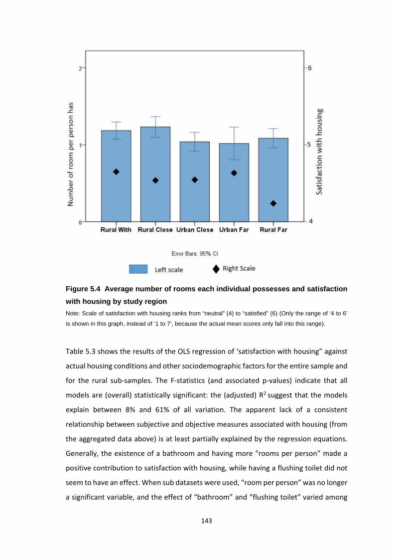
143

Figure 5.4 Average number of rooms each individual possesses and satisfaction with housing by study region Note: Scale of satisfaction with housing ranks from “neutral” (4) to “satisfied” (6) (Only the range of ‘4 to 6’

is shown in this graph, instead of ‘1 to 7’, because the actual mean scores only fall into this range).

Table 5.3 shows the results of the OLS regression of ‘satisfaction with housing” against

actual housing conditions and other sociodemographic factors for the entire sample and

for the rural sub-samples. The F-statistics (and associated p-values) indicate that all

models are (overall) statistically significant: the (adjusted) R2 suggest that the models

explain between 8% and 61% of all variation. The apparent lack of a consistent

relationship between subjective and objective measures associated with housing (from

the aggregated data above) is at least partially explained by the regression equations.

Generally, the existence of a bathroom and having more “rooms per person” made a

positive contribution to satisfaction with housing, while having a flushing toilet did not

seem to have an effect. When sub datasets were used, “room per person” was no longer

a significant variable, and the effect of “bathroom” and “flushing toilet” varied among

144

different areas. Again, the relationships between all the objective and subjective

indicators were mediated by sociodemographic factors.

Table 5.3 OLS regression results – with dependent variable being subjective measures of respondent satisfaction with housing

Variables

Total sample population

Urban Close

Rural with

Rural Close

Urban far

Rural Far

Bathroom 0.893*** 0.204 1.048** 0.986** 0.759 (0.295) (0.853) (0.417) (0.457) (1.091) Flushing toilet 0.241 1.301 –0.468 0.800 2.831** (0.294) (0.795) (0.409) (0.582) (1.279) Roomperperson 0.229** –0.024 0.155 0.278 –0.091 –0.356

(0.115) (0.270) (0.199) (0.238) (0.484) (0.663) NoOfChildren 0.041 0.173 –0.144 0.146 –0.848*** –0.152

(0.094) (0.258) (0.166) (0.140) (0.268) (0.411) NoOfAdult 0.055 0.002 –0.192** 0.235** 0.429** 0.006

(0.062) (0.117) (0.092) (0.109) (0.186) (0.280) Age 0.019** 0.055** 0.018 0.002 0.015 0.023

(0.008) (0.024) (0.013) (0.014) (0.032) (0.028) Female –0.356* –0.241 –0.279 –0.225 –0.750 –0.579

(0.183) (0.410) (0.289) (0.341) (0.523) (0.722) Not partnered –0.274 0.226 0.294 –1.193*** 1.277 0.230

(0.280) (0.602) (0.511) (0.417) (1.278) (1.068) Schooling –0.039 –0.065 –0.040 0.020 –0.125 –0.115 (0.030) (0.054) (0.052) (0.056) (0.118) (0.102)

Empl

oym

ent S

tatu

s

Retired 0.332 0.070 0.648 0.045 1.551 1.527 (0.362) (0.962) (0.559) (0.644) (1.357) (0.942)

Unemployed –0.332 –0.210 –0.590 0.060 –1.002 –0.709 (0.249) (0.839) (0.378) (0.464) (1.429) (0.845)

Student 0.880** 1.168* 1.006 0.810 0.137 1.539 (0.414) (0.594) (0.676) (0.734) (1.376) (1.212)

Self-employed

0.218 0.075 0.231 –0.068 1.957*** 0.611 (0.218) (0.479) (0.368) (0.381) (0.651) (0.759)

Constant 3.520*** 2.196 4.725*** 3.130*** 1.997 4.697* (0.601) (1.589) (0.996) (1.105) (2.162) (2.438) Observations 536 88 181 178 30 59

R2 0.075 0.356 0.133 0.12 0.61 0.116 F 4.32*** 6.82 2.26*** 2.58 14.08 1.32

Notes: 1. Robust standard errors are in parentheses; 2. Significant variables are highlighted in red,

***P<0.001,**p<0.05,*P<0.1.

145


relating to education

Figure 5.5 shows the percentage of respondents who had completed a certain level of

schooling across each type of study region. There is no obvious difference between coal

mining and non-coal mining areas, while urban areas had a larger proportion of

respondents with higher levels of education than did rural areas. That there is no

apparent relationship between mining and education should not be interpreted as

conclusive evidence of ‘no link’. Other Researchers who have examined the relationship

between resource dependence and education/human capital have used longitudinal or

time-series data at provincial (Zhan et al., 2015) or country level (Gylfason, 2001;

Gylfason and Zoega, 2006), and have used indicators such as public

expenditure/investment on education (Gylfason, 2001) or human capital (Zhan et al.,

2015)) and resource dependence rate (share of industrial output of mineral industries

in GDP (Zhan et al., 2015) or share of natural capital in national wealth (Gylfason, 2001;

Gylfason and Zoega, 2006)). Future research could thus seek to re-check the findings

using a more substantive data set.

Figure 5.5 Percentage of people with different education levels by study region

146

Means scores relating to respondent satisfaction with educational opportunities and

with the quality of education within regions are displayed in Figure 5.6. There is no

apparent difference in satisfaction with the education quality and education

opportunity between mining or non-coal mining areas. Interestingly, urban residents

were less satisfied with their educational opportunities than rural residents, with

significant differences between Urban Close and Rural With, Urban Close and Rural close

(see the result of Kruskal-Wallis test in Figure 4.4). This might be associated with the fact

that in urban areas, people have a preference for better schools but do not have equal

access to them. Those who were not able to be admitted to the ideal school experienced

“relative deprivation” – people felt deprived if they were doing less well than their

counterparts in the long term (Knight et al., 2009). In contrast, in rural areas, it was

common that several villages shared one school, and most rural residents confined their

reference group to the village (Knight et al., 2009), therefore, much less comparison was

involved. Compared Figure 5.5 and Figure 5.6, there is no obvious relationship between

these objective and subjective indicators of education were found.

147

Figure 5.6 Satisfaction with education opportunity and quality by study region

Note: Scale of satisfaction with education opportunity and quality ranks from “dissatisfied” (2) to “satisfied”

(6), 4 indicates “neutral” (Only the range of ‘2 to 6’, instead of ‘1 to 7’, is shown in this graph, because the

actual mean scores only fall into this range).

The results of OLS regression (see Appendix C-4 ) also indicates that objective indicators

of education (years of schooling of individuals) were not a significant contributor to

satisfaction with education opportunity and education quality, for any of the datasets

considered and the explanatory ability of these models was very low compared to the

models above.


The objective indicators considered above suggest that coal mining has a significant

negative impact on air quality and a significant positive impact on housing conditions

(high percentage of bathroom and flushing toilet). There was not, however, a discernible

148

link between other objective indicators of wellbeing and the coal mining intensity of the

study regions, including income, and perhaps education. There were, however,

significant and discernible differences in the objective indicators relating to family

income, housing and education between urban and rural areas. This finding is consistent

with the findings of others (Davey and Rato, 2012), further confirming the vast

urban/rural divide in China. Coal mining does not seem to help minimize the gap

between urban and rural areas, except for living conditions.

While some objective indicators of wellbeing are relatively easy to obtain and track in

time (e.g. those relating to income), such indicators are not always collected for some

wellbeing factors (e.g. factors relating to social capital). As discussed in section 2.3.1.3,

central data collection agencies do not generally collect ‘subjective’ data, so it can be

particularly difficult to access subjective indicators for numerous wellbeing factors. Until,

and unless, one is able to access both objective and subjective indicators, over time,

across numerous domains, we can only work with admittedly sub-standard data to draw

whatever inferences we can about the extent to which the two sets of wellbeing

indicators are aligned and if OWB can be used to infer SWB or vice versa.

In this study, I assessed the relationship between 4 different pairs of subjective and

objective indicators. When using aggregated data, it was clear that higher levels of actual

family income were associated with higher satisfaction with income, and that higher

levels of PM10 were associated with lower satisfaction with air quality. When using

individual data (in the regression analyses) and controlling for sociodemographic factors,

it was revealed again, that objective indicators of annual family income and air quality

(PM10) were generally good predictors of subjective satisfaction with family income and

air quality, respectively – although these relationships were partially mediated by

sociodemographic factors.

Generally, objective indicators of housing were not very good predictors for subjective

satisfaction with housing: there were no consistency between these indicators when

using aggregated data; when using individual data, the existence of flushing toilets and

number of rooms per person were not good predictors of satisfaction with housing,

while having a bathroom seemed to indicate high satisfaction with housing – again,

149

these relationship were partially mediated by sociodemographic factors. No matter if

using aggregated or individual data, subjective and objective indicators relating to

education did not seem to be portraying similar types of information.

To briefly recap key results relating to the ‘impact’ of mining on wellbeing: it matters

not whether one considers objective or subjective indicators, there is no apparent

relationship between coal mining and family income. Average family incomes, and

average ‘satisfaction’ with family incomes are similar in mining and non-mining regions.

This is despite the fact that coal mining is said to be a significant contributor to the local

economy (Editor of Land & Resource Herald, 2013), and despite the fact that those who

work in the mining industry earn, on average, higher incomes than those who work in

other industries (see Table 3.9 and Appendix B). Evidently, for every family within a coal-

mining region who has someone works in the industry and brings home an inflated

income, there is another ‘matching’ family that is not associated with the mining

industry and brings home a deflated income (so on average, they balance out). But that

begs a more sophisticated investigation – given over to chapter 6.

Objective and subjective indicators also tell a consistent – although entirely negative –

story about the impact of mining on air quality. Coal mining had negative impacts on air

quality (higher level of PM10 and lower level of satisfaction with air quality in coal mining

areas than non-coal mining areas). These findings are also consistent with the findings

of other researchers (e.g. Zullig and Hendryx, 2010; Bian et al., 2010; Colagiuri et al.,

2012).

Coal mining may also have positive impacts on housing conditions. This is only revealed

by the objective indicators considered here – but is supported by findings from the

broader literature (Zhang et al., 2015).

When looking at the relationship between objective and subjective indicators, it seems

that objective indicators can be used to predict satisfaction for some wellbeing factors,

but not for others. This is consistent with the findings of Emmons and Diener (1985).

They suggested that one might expect there to be different, and potentially

unpredictable relationships between objective and subjective indicators because some

of the ‘domains’ that contribute to wellbeing may be more (or less) inherently satisfying

150

than others. In this study, housing conditions were consistently given relatively high

satisfaction scores (see Figure 5.4, satisfaction scores with housing were all above 4

(neutral)), indicating that housing might be one of those such domains. Davey and Rato

(2012) also confirmed that rural residents in China were generally satisfied with their

living standards despite the low life quality in objective terms.

The inconsistency between objective and subjective indicators of housing partially

reflect the inadequacy of the objective measurements of wellbeing: they may, quite

simply, reflect too narrow a lens on what constitutes ‘wellbeing’. For example, good

housing conditions are not only reflected in the existence of bathrooms and flushing

toilets and more rooms: other factors, such as dampness, and the quality of construction,

will also influence people’s satisfaction with their housing, and thus ultimately their

wellbeing. Anecdotal evidence suggested that people from coal mining areas were

concerned with the safety of their houses due to the likely subsidence caused by coal

mining, which might partly explain why they were not significantly more satisfied with

their housing despite the fact that they had ‘better’ housing (measured by objective

indicators used here and OECD (2011)) than those living far away from coal mines. Until

or unless one is able to obtain more ‘objective’ data describing a broader range of

factors that contribute to housing quality, it seems as if subjective measures (which will

likely encompass the other, difficult-to-measure factors) are likely defensible indicators

of the housing quality and of the contribution that good quality housing makes to overall

wellbeing.

Even without this ‘scope’ issue (where an indicator of satisfaction likely encompasses a

broader range of factors than those captured by a single objective indicator), it will not

always be the case that subjective and objective indicators exactly align and measure

the same thing. In this study, the subjective indicator relating to education was defined

in terms of educational opportunity/quality and it may thus capture aspects of

institutional capital; in contrast educational attainment (the ‘objective’ measure used in

this study) is more likely an indicator of human capital (e.g. Frey & Stutzer, 1999; Di Tella

et al., 2003; Lange and Topel, 2006; Smyth et al., 2011). Misalignment of indicators thus

likely explains the lack of correlation between them. A better-matched subjective

indicator of educational attainment might instead be ‘how satisfied are you with your

151

education level?’ Although such a question might better match the objective indicator,

it would not convey much valuable information about education quality, opportunity

and/or concerns with the education system – again suggesting that comprehensive

assessments of wellbeing are probably best undertaken with a mix of subjective and

objective indicators.

The link between objective and subjective indicators might also ‘break down’ for other

reasons. For example, air quality or many other objective indicators (Oswald and Wu,

2010) are not always available at smaller geographic scales, so that researchers need to

use objective wellbeing data that have been collected at one scale, when making

comparisons with subjective wellbeing data that have been collected at another scale

(e.g. from individuals) (e.g. Schneider, 1975; Oswald and Wu, 2010). This is termed as

“scale discordance” by Lee and Marans (1980) – “a terms used to recognize that the

territorial base of an individual’s subjective evaluation may not coincidence with the

boundaries of the unities used for the collection of objective data” (Lee and Marans,

1980, p. 47). Lee and Marans (1980) also pointed out that scale discordance affects all

domains of wellbeing that incorporate a territorial component (e.g. satisfaction with air

quality in a village), and is one of the explanations for the imperfect relationship

between objective and subject measure of wellbeing.

As discussed in section 2.5.5, if researchers are interested in the wellbeing of people

from diverse regions (like those considered here – e.g. villages with or without mining),

then using highly aggregated objective wellbeing indicators at the county level (including

numerous villages) might eliminate those variations among villages and mask important

difference (Schneider, 1975). This is often referred to as ‘unobserved heterogeneity’.

Lee and Marans (1980) found that there would be a greater correlation between the

objective and subjective measures when the 2 sets of data are at a similar geographic

scale. Thus, it can be inferred that when examining the relationship between objective

and subjective measure of wellbeing that incorporate a territorial component,

maintaining the 2 sets of data at a similar geographic scale – and probably a smaller

scale as objective data collected from a large geographic area tend to mask more

heterogeneity – may reduce scale discordance and unobserved heterogeneity.

152

In this particular study, all the objective and subjective were collected at individual level

except air-quality measure, which was collected on the basis of locations (one reading

for one village or city). As a village in China is a much smaller geographic area than a city,

one can expect lower level of scale discordance and unobserved heterogeneity for

samples from villages than for samples from cities. However, it would have been present

if, for example, some respondents in a village lived up-wind from a coal mine, while

others lived down-wind. Future study may better investigate this issue using the air-

quality data with higher resolution (e.g. at individual household level).

In particular, objective indicators fall short when measuring attitudinal matters, such as

“trust” and “perceived safety” in the street (Veenhoven, 2002), that are considered as

indicators of social capital in this study and many other (e.g. Prewitt et al., 2014).

According to Prewitt et al. (2014), social capital can be measured by objective indicators

e.g. using network structures that link individuals (such as voluntary association

memberships); but these objective indicators are inherently different from subjective

indicators (such as measures of trust in others or of norms of reciprocity) and thus

measure different elements of social capital.


By exploring the impacts of coal mining using both objective and subjective indicators,

this chapter further confirms that coal mining does not have any obvious impacts on

income in host communities. Coal mining improves the living conditions, but it

dramatically affects the natural environment and people’s satisfaction with the natural

environment (air quality, in particular). Messages from objective data in this chapter

confirms the policy priority in coal mining areas should be addressing environmental

issues (air quality in particular), which is consistent with the finding from the previous

chapter using subjective data.

The analysis of this chapter also demonstrates that despite the fact that objective

indicators are considered by some to be ‘superior’ indicators, and that they are based

upon objectively verifiable data, they are not unambiguously ‘better’. This analysis

illustrates that not only do subjective wellbeing indicators provide feedback about, for

153

example, the level of satisfaction of local residents with existing conditions, but they

also provide information about some factors which objective indicators are unable to

adequately capture. While objective indicators provide useful information, they also

omit important aspects of wellbeing, especially when single, aggregated measures, mask

differences within regions, and are not able to reveal information about people’s

preferences.

It seems that subjective indicators are an important complement to objective indicators

when seeking to describe, measure and/or explain wellbeing, and thus inform public

policy. The consistency between objective and subjective indicators of air quality and

income indicates that it might be appropriate to choose any of them to measure these

indicators. Notably, since this relationship between objective and subjective is partially

mediated by sociodemographic factors, it is thus correct to say that improvements in

household income (or reduction in PM10, or in the number of houses that have

bathrooms) will be accompanied by improvements in people’s satisfaction with their

income (or air quality or housing). But it does not necessarily mean people who have

high income (or good air quality, or a bathroom in their housing) will be more satisfied

with their income (or air quality, or house) than others with lower income (or with poor

air quality or no bathroom).

For other wellbeing indicators, where the objective indicators are not good predictors

of subjective indicators, both may be needed to inform public policy (in this case,

improvements measured by objective indicators are not always reflected with

improvements in satisfaction).


Not only does this chapter illustrate that objective and subjective indicators do not

always convey consistent messages (thus demonstrating the utility of subjective

indicators to inform public policy), but it also demonstrates empirical approaches to

examine the relationship between these 2 sets of indicators. Using these approaches,

future studies can examine the relationship between objective and subjective indicators

relating to other wellbeing factors and in other social contexts. The general approaches

154

then enable researchers or decision makers to decide when (in which regions, and for

which factors/domains) it may be appropriate to use only objective indicators, when it

may be appropriate to use subjective indicators, and when it might be necessary to use

both. This study also offers direction for future studies to better investigate the

relationship between these 2 measures of wellbeing. For example, future studies can

control for sociodemographic factors, align the scope of these 2 measures and use data

with higher resolution (e.g. at individual level) to reduce the scale discordance and

unobserved heterogeneity.


As noted earlier, when working with regional environmental data, unobserved

heterogeneity occurs when a person living in one part of a region experiences different

conditions to those of someone living elsewhere in that region (Welsch, 2006), which

might be one of the issues that affect the relationship between objective and subjective

indicators. This exploratory investigation into the relationship between PM10 and

satisfaction with air quality did not address that potential problem, like many/most

other life satisfaction studies (e.g. Welsch, 2006). Using time-series data, some studies

that have sought to investigate the relationship between air pollution and life

satisfaction have demonstrated techniques for dealing with the problem of unobserved

heterogeneity by, for example, including distance from central business district

(MacKerron & Mourato, 2009) or distance from air monitoring system (Ferreira et al.,

2013). Future studies could thus usefully consider the link between subjective and

objective measures of air quality, using such techniques or data at individual level to

control for unobserved heterogeneity and generating results that could be treated with

more confidence.

The relationship between objective and subjective indicators of wellbeing might be

different in different cultures/settings, suggesting the need for further research to

confirm or refute findings here in other social contexts. Further research could also

explore relationships between more objective and subjective indicators to inform public

policies.

155

Thesis outline

156

6. CHAPTER 6 IMPACTS OF COAL MINING ON

SUBJECTIVE WELLBEING: USING THE LIFE SATISFACTION

APPROACH

Chapter outline

6.1 Introduction


6.2.1 Assessing the impacts of coal mining on different life domains

6.2.2 Assessing the impacts of coal mining on global life satisfaction

6.3 Results

6.3.1 Determinants of satisfaction with life domains

6.3.2 Impacts of coal mining on global life satisfaction





157

Synopsis

This chapter uses more sophisticated techniques than those employed in chapter 4 to

test for statistically significant ‘impacts’ of coal mining on subjective wellbeing –

considering impacts on satisfaction with different life domains and on global life

satisfaction (GLS). Life satisfaction models were developed to generate empirical results

– essentially regressing satisfaction (with a particular life domain, or with life overall)

against numerous sociodemographic factors known to influence life satisfaction, and

also variables capturing mining intensity.

Coal mining was found to have statistically discernible impacts on satisfaction with

various life domains in host communities. Strong evidence is found to support previous

‘suggestive’ results, namely that: those living in rural coal mining areas were less

satisfied with the natural environment, the economy and society than those living in

rural areas disassociated from mining. Evidence was also found to suggest that those

living in rural coal mining areas were generally more satisfied with their living conditions

than those living further away from the mines. So there are clearly some ‘costs’ and

some ‘benefits’.

The analysis of overall life satisfaction allowed for an assessment of ‘net’ impacts on

host communities – statistically significant, and negative in rural areas with coal mining.

It was found that those living in rural areas with coal mining were less satisfied with life

overall, than those living further away (either near or far away). I was able to use

coefficients from the model to infer that if one wished to ensure that these ‘unsatisfied’

people were given enough money to raise their satisfaction to a similar level as those

living further away, then those people would need, on average, 20,000 Yuan per annum.

The analysis also demonstrated that those who were dependent upon coal mining for

their household income, were much more satisfied with life overall, than those who

lived in the same village, but were dependent upon other industries. The models suggest

that if one wished to ensure that these ‘unsatisfied’ people were given enough money

to raise their satisfaction to a similar level as those who depend upon the mining

industry for their household income, then they would need, on average, 47,000 per

annum. These models used to generate these estimates are, like most models,

158

inherently imperfect – so results should be treated with caution: generating indicative,

rather than precise estimates of ‘net impact’.

159

6.1 Introduction

Current methods for conducting mining impact assessments, such as environmental

impact assessment, social impact assessment and economic impact assessment are

limited in their ability to simultaneously assess a large variety of non-market impacts

associated with of coal mining. It is thus difficult to adequately assess trade-offs

associated with mining (e.g. potential increases in income weighed against negative

impacts on air quality). Although market-based (MB) approaches, revealed preference

(RP) and stated preference (SP) have been used to assess some of the impacts associated

with mining (e.g. Trigg and Dubourg, 1993; Ivanova et al., 2007; Gillespie and Kragt, 2010;

Li et al., 2011), the methodological techniques constrain researchers to consider only a

small number of impacts. The life satisfaction (LS) approach, which may avoid some of

those disadvantages, has not previously been used to assess impacts of mining. Thus,

this chapter uses the LS approach to assess the multiple impacts of coal mining, the

ultimate aim being to provide better information about the impacts of coal mining on

different life domains, and on the quality of life overall.

Most apparent from the literature review in chapter 2, is that numerous factors

influence GLS – these include, but are not limited to things such as satisfaction with

particular life domains, location (e.g. rural/urban) and a range of sociodemographic

factors such as age, gender, education, and marital status. Table 3.9 in chapter 3, clearly

shows that the sociodemographic characteristics of the different sub-samples included

in this study varied significantly; there were, for example, a higher percentage of males

included in the Rural With sample (47%), than in the Rural Close or Rural Far samples

(approx. 36% each). Since sociodemographic variables influence GLS (and satisfaction

with life domains – as shown in chapter 5), it is not strictly valid to simply compare GLS

(or satisfaction with particular life domains) across regions, attributing differences to

rural/urban local or to distance from coal mines. One needs to determine if there are

differences in GLS (or satisfaction with particular life domains) across regions with

different intensities of mining, after having controlled for differences associated with

‘confounding’ factors (such as age and gender).

160

The overarching research question addressed in this chapter is thus: Is it possible to

quantify the net impacts of coal mining (on broad ‘domains’ of life and on the overall

wellbeing of host communities) and to determine how much should, in principle, be paid

‘in compensation’ to those who are, overall, impacted negatively? It is answered by

addressing the following sub-questions:

1) How does coal mining affect satisfaction with life domains (after controlling for


2) How does coal mining affect global life satisfaction (after controlling for


3) If the net impact of mining, on global life satisfaction, is negative, then how

much extra income would need to be paid to the negatively impacted people,

to raise their ‘satisfaction’ to the same level as their unaffected counterparts?

Methods used to analyse the data are described in section 6.2. Section 6.3 presents

results relevant to the research questions followed by a discussion in section 6.4.


The hypothesis underlying the investigations of this chapter is that a respondent’s stated

satisfaction (with a particular life domain or with life overall) will depend upon proximity

to coal mining, and to a range of other factors, relating to location (urban/rural) and to

the sociodemographic characteristics of respondents. To test this hypothesis, a series of

multiple regressions were conducted, using stated satisfaction (with particular life

domains, and later, with life overall) as the dependent variable, and including

sociodemographic variables as regressors – in addition to variables associated with

proximity to coal mining. Further details are given below.

6.2.1 Assessing the impact of coal mining on different life domains

6.2.1.1 Identifying ‘domains’ and dependent variables for use in regression equations

In theory, one could investigate the ‘impact’ of mining on each of the 29 different

wellbeing factors discussed in Chapter 4, using the life satisfaction approach. However,

161

as noted in chapter 2, many of those wellbeing factors are likely related. Several

researchers have undertaken analyses that have grouped the numerous factors

considered by researchers to influence wellbeing into a smaller subset of ‘domains (e.g.

Cummins, 1996; Larson et al., 2011, 2013, 2014). The general method used by these

researchers was the principal components analysis (PCA) with varimax rotation (e.g.

Larson et al., 2011, 2013, 2014), and it is the approach that was used in this study.

Specifically, I used PCA to identify factors that grouped together into common domains.

Having done this, I then sought to calculate a ‘score’ for each component (i.e. each life

domain). Scores can be calculated using a variety of approaches, the appropriateness

of which depends on context. There are two main classes of score computation: non-

refined and refined. Non-refined scores are computed using simple methods, such as

calculating the sum or average of all variables identified as belonging to a domain

(DiStefano et al., 2009). Refined scores, in contrast, are computed using more

sophisticated and technical methods, such as regression scores. In general, non-refined

scores are thought to be more stable across samples than refined methods (Grice &

Harris, 1998, cited by DiStefano et al., 2009); and sum/average scores are preferred

when undertaking exploratory research (Tabeachinck and Fidell, 2001 and Hair et al.,

2006, cited by DiStefano et al., 2009). Moreover, using an average score preserves

variation in the original data, helps retain the scale metric and fosters comparison across

factors (DiStefano et al., 2009). For these reasons, mean scores were used here.

Specifically, the mean score for each life domain was calculated by calculating the mean

of all factors within each domain that had a loading value above 0.3 – only using ‘marker’

factors with stronger loading to take into account a factor’s relationship to the life

domains (DiStefano et al., 2009). It is those means scores which are used as the

dependent variable in each regression equation.

An aggregated radar chart was created, showing scores for each ‘domain’ by study

region. This chart was compared with the chart from chapter 4 (Figure 4.4) to check for

observational consistency and to make a preliminary assessment about the way in which

these aggregated indicates of satisfaction with life domains differed across case-study

areas.

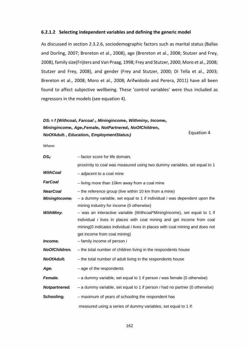
162

6.2.1.2 Selecting independent variables and defining the generic model

As discussed in section 2.3.2.6, sociodemographic factors such as marital status (Ballas

and Dorling, 2007; Brereton et al., 2008), age (Brereton et al., 2008; Stutzer and Frey,

2008), family size(Frijters and Van Praag, 1998; Frey and Stutzer, 2000; Moro et al., 2008;

Stutzer and Frey, 2008), and gender (Frey and Stutzer, 2000; Di Tella et al., 2003;

Brereton et al., 2008; Moro et al., 2008; Arifwidodo and Perera, 2011) have all been

found to affect subjective wellbeing. These ‘control variables’ were thus included as

regressors in the models (see equation 4).

DSi = f (Withcoali, Farcoal i, Miningincomei, Withminyi, Incomei, Miningincomei, Agei,Femalei, NotPartneredi, NoOfChildreni,

NoOfAdulti , Educationi, EmploymentStatusi)

Where:

Equation 4

DSij – factor score for life domainj

proximity to coal was measured using two dummy variables, set equal to 1

WithCoal – adjacent to a coal mine

FarCoal – living more than 10km away from a coal mine

NearCoal – the reference group (live within 10 km from a mine)

MiningIncomei – a dummy variable, set equal to 1 if individual i was dependent upon the

mining industry for income (0 otherwise)

WithMinyi – was an interactive variable (Withcoal*MiningIncome), set equal to 1 if

individual i lives in places with coal mining and get income from coal

mining(0 indicates individual i lives in places with coal mining and does not

get income from coal mining) Incomei – family income of person i

NoOfChildreni – the total number of children living in the respondents house

NoOfAdulti – the total number of adult living in the respondents house

Agei – age of the respondents

Femalei – a dummy variable, set equal to 1 if person i was female (0 otherwise)

Notpartneredi – a dummy variable, set equal to 1 if person i had no partner (0 otherwise)

Schoolingi – maximum of years of schooling the respondent has

measured using a series of dummy variables, set equal to 1 if:

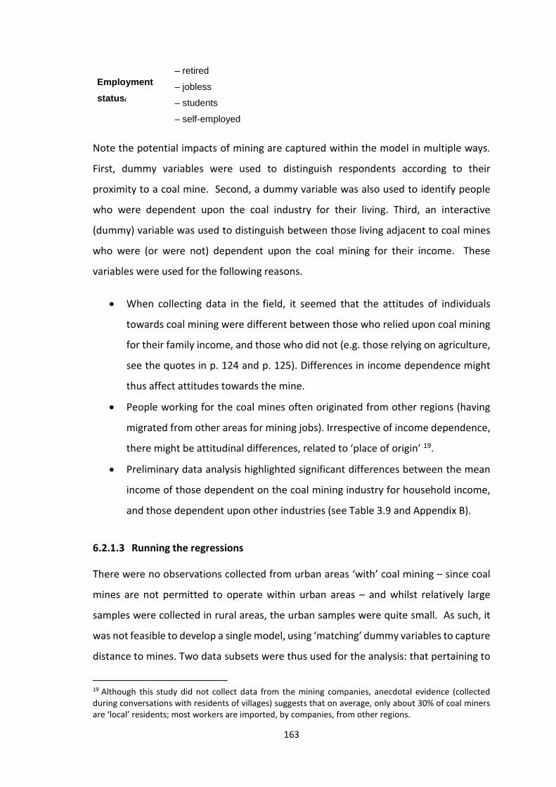
163

Note the potential impacts of mining are captured within the model in multiple ways.

First, dummy variables were used to distinguish respondents according to their

proximity to a coal mine. Second, a dummy variable was also used to identify people

who were dependent upon the coal industry for their living. Third, an interactive

(dummy) variable was used to distinguish between those living adjacent to coal mines

who were (or were not) dependent upon the coal mining for their income. These

variables were used for the following reasons.

• When collecting data in the field, it seemed that the attitudes of individuals

towards coal mining were different between those who relied upon coal mining

for their family income, and those who did not (e.g. those relying on agriculture,

see the quotes in p. 124 and p. 125). Differences in income dependence might

thus affect attitudes towards the mine.

• People working for the coal mines often originated from other regions (having

migrated from other areas for mining jobs). Irrespective of income dependence,

there might be attitudinal differences, related to ‘place of origin’ 19.

• Preliminary data analysis highlighted significant differences between the mean

income of those dependent on the coal mining industry for household income,

and those dependent upon other industries (see Table 3.9 and Appendix B).

6.2.1.3 Running the regressions

There were no observations collected from urban areas ‘with’ coal mining – since coal

mines are not permitted to operate within urban areas – and whilst relatively large

samples were collected in rural areas, the urban samples were quite small. As such, it

was not feasible to develop a single model, using ‘matching’ dummy variables to capture

distance to mines. Two data subsets were thus used for the analysis: that pertaining to

19 Although this study did not collect data from the mining companies, anecdotal evidence (collected during conversations with residents of villages) suggests that on average, only about 30% of coal miners are ‘local’ residents; most workers are imported, by companies, from other regions.

Employment statusi

– retired

– jobless

– students

– self-employed

164

data collected from urban areas, and that collected from rural areas. Not only does this

simplify the analysis, and allow one to explicitly allow for differences in coefficients

between rural and urban areas, but it allows for a focus on rural areas, which are more

closely exposed to the impacts of coal mines than urban areas, and which are the core

major interest of this study. This approach is also in line with other studies of wellbeing

in China which usually differentiate urban (Appleton and Song, 2008; Smyth et al., 2011)

and rural areas (Knight et al., 2009).

As discussed in the preceding chapter, ordinary least squares (OLS) regression was

designed for a continuous, and normally distributed, dependent variable. The factors

scores used to here does not strictly satisfy that assumption (although using mean factor

scores rather than Likert data markedly reduces, if not eliminates, the problem of

categorical data). So in the first instance, both OLS and ordinal regression were run. As

was the case for chapter 5 (section 5.2), and has been the case in many other studies

cited in section 5.2, differences between OLS and the models were negligible20. So OLS

was thus used for primary analysis, results from the ordinal regression were used as a

cross-reference and robustness check.

6.2.1.4 Using coefficients to draw inferences about the impacts of mining on

satisfaction with life domains

In urban areas, there were only two groups (Urban Close and Urban Far). A single

dummy variable (‘FarCoal’) can distinguish between the two, with the reference group

being Urban Close (‘NearCoal’). This means it is possible to simply inspect the coefficient

on the identifying dummy variable (‘FarCoal’), determining if it was statistically

significant, and (if so) if the presence of mining had a positive or negative impacts on

satisfaction with particular life domains (after having controlled for all other factors).

In rural areas, however, there were three groups (Rural With, Rural Close and Rural Far).

The reference group is Rural close (‘NearCoal’), which means that it is possible to tell if

there are statistically significant differences in the satisfaction with particular domains

20 See Appendix D-1 for results of ordinal regressions examining the determinants of satisfaction with life domains.

165

between those living Rural With and Rural Close, by examining the coefficient on the

dummy variable ‘WithCoal’. Similarly, it is possible to tell if there are statistically

significant differences in the satisfaction with each domain between those living in Rural

Far and Rural Close by examining the coefficient on ‘FarCoal’. However, post-estimation

tests must be undertaken to assess differences between Rural with and Rural Far, by

examining the coefficients ‘WithCoal’ and ‘FarCoal’.

To explain, consider the following simple equation describing the relationship between

the variable of ‘WithCoal’ and ’FarCoal’. If the coefficients on the two variables are

identical, then the difference between the two will be zero. The hypothesis underlying

post-estimation tests is thus that there is no significant difference between the

coefficients of these 2 variables, i.e. that:

β1WithCoalj - β2FarCoalj=0 Equation 5

Where: β1 = the coefficients of ‘WithCoal’ from the results of Equation 4 β2 = the coefficients of ‘FarCoal’ from results of Equation 4

The statistical packaged used to analyse data (STATA) has an in-built post-estimation

test that allows one to specify such a null hypothesis, and it is that which was used here.

6.2.2 Assessing the impacts of coal mining on global life satisfaction

6.2.2.1 Preliminary analysis of the dependent variable and its relation to mining

As stated in section 3.4.1, the questionnaire collected data relating to GLS using two

different methods: the 0 – 100 scale, similar to Cantril’s Ladder (Cantril, 1965) and the

Satisfaction With Life Scale (SWLS) (Diener et al., 1985). To determine which measure

would be better to use in the regression analysis, the consistency of responses across

the two measures at both a regional level (by observing the mean values across 5 regions)

were firstly looked at. Then the consistency of responses at an individual level was also

looked at (checking correlation). Since the 2 measurements of global life satisfaction

seem to provide similar information, the finer-scale measure of GLS (specifically, the LS

rating (0 – 100)) was selected for use in the subsequent analyses.

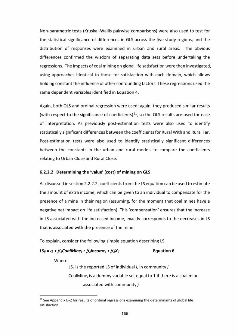
166

Non-parametric tests (Kruskal-Wallis pairwise comparisons) were also used to test for

the statistical significance of differences in GLS across the five study regions, and the

distribution of responses were examined in urban and rural areas. The obvious

differences confirmed the wisdom of separating data sets before undertaking the

regressions. The impacts of coal mining on global life satisfaction were then investigated,

using approaches identical to those for satisfaction with each domain, which allows

holding constant the influence of other confounding factors. These regressions used the

same dependent variables identified in Equation 4.

Again, both OLS and ordinal regression were used; again, they produced similar results

(with respect to the significance of coefficients)21, so the OLS results are used for ease

of interpretation. As previously post-estimation tests were also used to identify

statistically significant differences between the coefficients for Rural With and Rural Far.

Post-estimation tests were also used to identify statistically significant differences

between the constants in the urban and rural models to compare the coefficients

relating to Urban Close and Rural Close.

6.2.2.2 Determining the ‘value’ (cost) of mining on GLS

As discussed in section 2.2.2.2, coefficients from the LS equation can be used to estimate

the amount of extra income, which can be given to an individual to compensate for the

presence of a mine in their region (assuming, for the moment that coal mines have a

negative net impact on life satisfaction). This ‘compensation’ ensures that the increase

in LS associated with the increased income, exactly corresponds to the decreases in LS

that is associated with the presence of the mine.

To explain, consider the following simple equation describing LS.

LSij = α + β1CoalMinej + β2IncomeI + β3XIj Equation 6

Where: LSij is the reported LS of individual i, in community j

CoalMinej is a dummy variable set equal to 1 if there is a coal mine

associated with community j

21 See Appendix D-2 for results of ordinal regressions examining the determinants of global life satisfaction.

167

Incomej is the income of individual i, in community j

Xij is a vector of the other variables known to influence LS

β1 = MC CoalMine is the impact of a coal mine on LS

β2 = MBIncome is the (marginal) impact of additional income on LS

Holding all ‘confounding’ factors constant, the difference in LS between an individual

living in a region that has a coal mine, and an ‘identical’ individual (e.g. same

sociodemographic, same income) who lives in a region without a coal mine is β1. So if a

mine were to ‘appear’ in a region that previously did not have one, the model predicts

that LS would go down by β1. Each unit of income (RMB) gives an extra ‘β2 ’ units of LS.

So one could ‘compensate’ for the mine, by giving each individual within that region an

increase in income = β1/β2 (termed the marginal rate of substitution = marginal disutility

of mining / marginal utility of income).

This approach to assessing, and then comparing, the marginal disutility of a range of

public ‘bads’ with the marginal utility of income has been used in many studies focusing

on: airport noise (Van Praag and Baarsma, 2004), air pollution (Welsch, 2006; Luechinger,

2009; MacKerron and Mourato, 2009), terrorism (Frey et al., 2009), corruption (Welsch,

2008) and disasters (Luechinger and Raschky, 2009). Some have even proposed a

compensation scheme using the results of LS studies to compensate those experiencing

reduced wellbeing from public ‘bads’ (e.g. airport noise (Van Praag and Baarsma, 2005)).

A similar approach is thus used here, to assess the extent to which proximity to coal

mining affects GLS, and to calculate the income that would be required to ‘compensate’

people for any negative impacts, although such calculations were done relative to the

‘reference group’ (e.g. those living near coal).

Here

• The amount of income that would need to be paid to ‘compensate’ someone

who lived ‘with coal’, compared to those who lived ‘near coal’, is calculated as:

MRS=–𝜕𝜕𝜕𝜕𝜕𝜕𝜕𝜕/𝜕𝜕𝜕𝜕𝜕𝜕𝜕𝜕ℎ𝐶𝐶𝐶𝐶𝐶𝐶𝐶𝐶𝜕𝜕𝜕𝜕𝜕𝜕𝜕𝜕/𝜕𝜕𝜕𝜕𝜕𝜕𝜕𝜕𝐶𝐶𝜕𝜕𝜕𝜕

=–𝜕𝜕𝜕𝜕𝜕𝜕𝜕𝜕ℎ𝐶𝐶𝐶𝐶𝐶𝐶𝐶𝐶𝜕𝜕𝜕𝜕𝜕𝜕𝜕𝜕𝐶𝐶𝜕𝜕𝜕𝜕

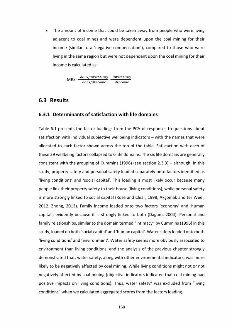
168

• The amount of income that could be taken away from people who were living

adjacent to coal mines and were dependent upon the coal mining for their

income (similar to a ‘negative compensation’), compared to those who were

living in the same region but were not dependent upon the coal mining for their

income is calculated as:

MRS=–𝜕𝜕𝜕𝜕𝜕𝜕𝜕𝜕/𝜕𝜕𝜕𝜕𝜕𝜕𝜕𝜕ℎ𝑀𝑀𝜕𝜕𝜕𝜕𝑀𝑀𝜕𝜕𝜕𝜕𝜕𝜕𝜕𝜕/𝜕𝜕𝜕𝜕𝜕𝜕𝜕𝜕𝐶𝐶𝜕𝜕𝜕𝜕

=–𝜕𝜕𝜕𝜕𝜕𝜕𝜕𝜕ℎ𝑀𝑀𝜕𝜕𝜕𝜕𝑀𝑀𝜕𝜕𝜕𝜕𝜕𝜕𝜕𝜕𝐶𝐶𝜕𝜕𝜕𝜕

6.3 Results

6.3.1 Determinants of satisfaction with life domains

Table 6.1 presents the factor loadings from the PCA of responses to questions about

satisfaction with individual subjective wellbeing indicators – with the names that were

allocated to each factor shown across the top of the table. Satisfaction with each of

these 29 wellbeing factors collapsed to 6 life domains. The six life domains are generally

consistent with the grouping of Cummins (1996) (see section 2.3.3) – although, in this

study, property safety and personal safety loaded separately onto factors identified as

‘living conditions’ and ‘social capital’. This loading is most likely occur because many

people link their property safety to their house (living conditions), while personal safety

is more strongly linked to social capital (Rose and Clear, 1998; Akçomak and ter Weel,

2012; Zhong, 2013). Family income loaded onto two factors ‘economy’ and ‘human

capital’; evidently because it is strongly linked to both (Dagum, 2004). Personal and

family relationships, similar to the domain termed “intimacy” by Cummins (1996) in this

study, loaded on both ‘social capital’ and ‘human capital’. Water safety loaded onto both

‘living conditions’ and ‘environment’. Water safety seems more obviously associated to

environment than living conditions, and the analysis of the previous chapter strongly

demonstrated that, water safety, along with other environmental indicators, was more

likely to be negatively affected by coal mining. While living conditions might not or not

negatively affected by coal mining (objective indicators indicated that coal mining had

positive impacts on living conditions). Thus, water safety” was excluded from “living

conditions” when we calculated aggregated scores from the factors loading.

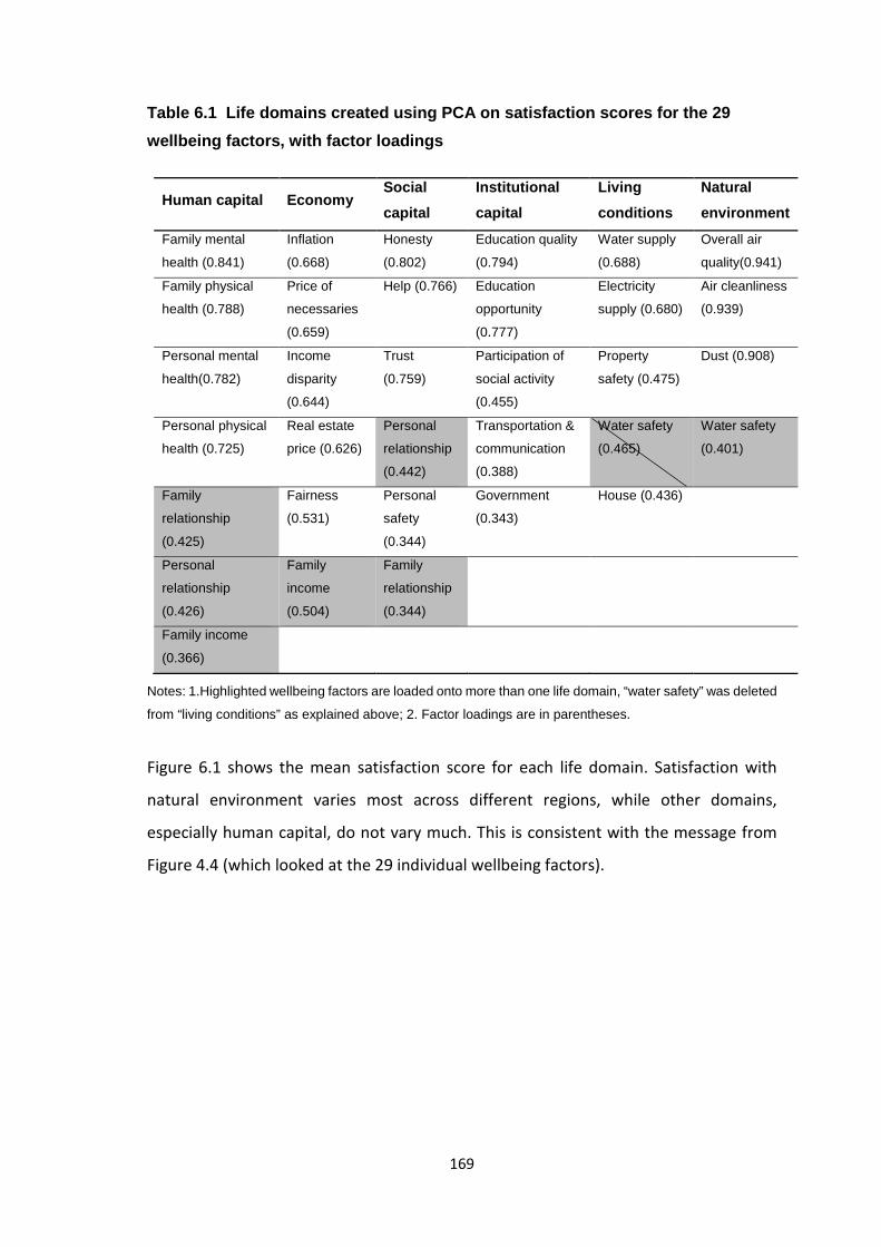
169

Table 6.1 Life domains created using PCA on satisfaction scores for the 29 wellbeing factors, with factor loadings

Human capital Economy Social capital

Institutional capital

Living conditions

Natural environment

Family mental

health (0.841)

Inflation

(0.668)

Honesty

(0.802)

Education quality

(0.794)

Water supply

(0.688)

Overall air

quality(0.941)

Family physical

health (0.788)

Price of

necessaries

(0.659)

Help (0.766) Education

opportunity

(0.777)

Electricity

supply (0.680)

Air cleanliness

(0.939)

Personal mental

health(0.782)

Income

disparity

(0.644)

Trust

(0.759)

Participation of

social activity

(0.455)

Property

safety (0.475)

Dust (0.908)

Personal physical

health (0.725)

Real estate

price (0.626)

Personal

relationship

(0.442)

Transportation &

communication

(0.388)

Water safety

(0.465)

Water safety

(0.401)

Family

relationship

(0.425)

Fairness

(0.531)

Personal

safety

(0.344)

Government

(0.343)

House (0.436)

Personal

relationship

(0.426)

Family

income

(0.504)

Family

relationship

(0.344)

Family income

(0.366)

Notes: 1.Highlighted wellbeing factors are loaded onto more than one life domain, “water safety” was deleted

from “living conditions” as explained above; 2. Factor loadings are in parentheses.

Figure 6.1 shows the mean satisfaction score for each life domain. Satisfaction with

natural environment varies most across different regions, while other domains,

especially human capital, do not vary much. This is consistent with the message from

Figure 4.4 (which looked at the 29 individual wellbeing factors).

170

Figure 6.1 Satisfaction with life domains

Note: Scale ranks from “very dissatisfied” (1) to “very satisfied” (7), 4 indicates “neutral”.

Table 6.2 presents the results from the regressions that sought to determine if mining

impacted particularly life domains, holding constant other potentially confounding

factors. Overall, most of the models were statistically significant, although the

explanatory power of these models is not high. Income had a positive impact on

(satisfaction with) human capital and on the economy in both urban and rural areas, and

with living conditions in rural areas. Age had positive impact on some life domains.

Females were less satisfied with institutional capital than males in rural areas. Students

were more satisfied with some life domains than those who were working. Years of

schooling is inversely correlated with (satisfaction with) living conditions and the

environment in rural areas. The number of children and/or adults living in the house and

marital status are not significant in any of the models.

As shown in Table 6.2, in rural areas, those living far away from coal mines reported high

levels of satisfaction with the human capital, economy, institutional capital, and

environment than rural residents living close to coal mines; they, however, reported

lower levels of satisfaction with their living conditions. In urban areas, those living far

1

2

3

4

5

6

7Human capital

Natrualenvironment

Economy

Social capital


Living conditions


171

away from coal mines reported higher levels of satisfaction with institutional capital and

the environment than those living close to coal mines.

Notably, rural residents living near coal mines (the reference group), were less satisfied

with the natural environment than those living far from coal, and more satisfied than

those living in rural areas with coal mining. MacKerron and Mourato (2009) simply

compared the effect of NO2 on LS (measured by a 11-point scale) to other studies that

using different scales to measure LS (e.g. Welsch (2003), in which LS was measured by a

4-point scale). Since all the dependent variables in Table 6.2 are measured by a similar

7-point rating scale, and independent variables of all the models are uniform, the

comparison between coefficients of different models is more straightforward.

Coefficients within the environmental domain appear to be larger than those relating to

any other life domain, indicating that coal mining has stronger impacts on satisfaction

with environment than on other domains.

172

Table 6.2 Results from OLS regression of factor scores (relating to satisfaction with different life domains) and other variables (sociodemographic factors and proximity to coal mines)

Human capital Economy Social capital Institutional capital Living conditions Natural environment Urban Rural Urban Rural Urban Rural Urban Rural Urban Rural Urban Rural

WithCoal 0.129 –0.147 –0.029 0.096 –0.187 –.738*** (0.116) (0.141) (0.118) (0.141) (0.141) (0.186) FarCoal 0.037 0.231* 0.250 0.456*** 0.269 0.206 0.521** 0.321* 0.321 –0.632*** 1.112*** 2.048*** (0.170) (0.133) (0.247) (0.158) (0.223) (0.137) (0.221**) (0.168) (0.237) (0.180) (0.344) (0.228) MiningIncome 0.059 0.216 –0.070 –0.051 –0.185 0.123 0.657** 0.181 0.095 0.036 0.725** –0.266 (0.245) (0.212) (0.250) (0.233) (0.244) (0.213) (0.284) (0.209) (0.266) (0.226) (0.354) (0.303) WithMiny –0.180 0.466 –0.130 0.042 0.205 0.173 (0.258) (0.281) (0.261) (0.274) (0.272) (0.352) Income 6.25E–06*** 5.78E–06** 0.0000101*** 0.0000103*** 2.50E–06 4.69E–07 1.3E–06 3.82E–06 4.59E–06 5.24E–06** 4.76E–06 5.24E–06 (2.23E–06) (2.33E–06) (3.01E–06) (2.05E–06) (2.53E–06) (2.12E–06) (2.4E–06) (2.38E–06) (3.32E–06) (2.44E–06) (4.30E–06) (2.44E–06) NoOfChildren 0.029 –0.007 0.153 0.041 0.085 –0.020 –0.082 –0.063 –0.185 –0.053 –0.256 0.007 (0.119) (0.053) (0.152) (0.055) (0.114) (0.058) (0.122) (0.065) (0.178) (0.058) (0.186) (0.007) NoOfAdult 0.052 0.009 0.146 –0.048 0.001 0.006 0.032 0.013 0.089 0.003 –0.050 0.010 (0.057) (0.036) (0.095) (0.037) (0.060) (0.042) (0.070) (0.039) (0.075) (0.039) (0.112) (0.153) Age 0.015 0.007 0.007 0.012** 0.000 0.013** 0.014 0.004 0.022* 0.005 0.004 0.054 (0.009) (0.004) (0.011) (0.006) (0.008) (0.005) (0.011) (0.006) (0.012) (0.005) (0.015) (0.052) Female 0.193 –0.031 0.019 –0.094 –0.175 –0.005 –0.192 –0.339*** –0.223 –0.173 –0.297 0.172 (0.184) (0.109) (0.218) (0.121) (0.181) (0.104) (0.196) (0.125) (0.250) (0.117) (0.316) (0.237) NotPartnered 0.435* –0.232 –0.275 0.153 –0.010 –0.105 –0.251 –0.013 –0.110 –0.079 –0.349 –0.005 (0.230) (0.166) (0.263) (0.181) (0.227) (0.154) (0.253) (0.177) (0.322) (0.181) (0.378) (0.073) Schooling –0.007 –0.004 –0.007 –0.030 –0.044 –0.003 –0.021 0.014 –0.037 –0.056*** –0.001 –0.096*** (0.025) (0.017) (0.036) (0.019) (0.227) (0.017) (0.034) (0.021) (0.034) (0.019) (0.046) (0.028)

Empl

oym

ent

Stat

us

Retired 0.369 0.152 –0.064 0.215 0.890** –0.182 0.057 0.101 0.177 0.116 1.584*** –0.274

(0.427) (0.202) (0.526) (0.242) (0.380) (0.201) (0.579) (0.263) (0.511) (0.220) (0.581) (0.320)

Unemployed 0.155 –0.330** 0.538 –0.178 0.136 –0.001 –0.115 –0.013 –0.403 –0.118 0.659 –0.005

(0.304) (0.147) (0.428) (0.158) (0.416) (0.142) (0.349) (0.159) (0.536) (0.167) (0.548) (0.197)

Student –0.187 0.029 1.097*** 0.155 0.487 –0.133 1.103*** –0.752** 1.367*** 0.514** 0.871** 0.890** (0.309) (0.273) (0.321) (0.260) (0.297) (0.234) (0.269) (0.358) (0.361) (0.255) (0.408) (0.402)

Self-employed

0.276 0.013 0.136 –0.120 0.202 –0.128 –0.058 –0.044 0.353 0.087 –0.228 0.127 (0.235) (0.117) (0.274) (0.147) (0.222) (0.124) (0.253) (0.148) (0.283) 0.144 (0.348) (0.188)

Constant 4.201*** 5.092*** 1.755** 2.874*** 4.873*** 4.777*** 3.243*** 3.845*** 3.595*** 5.107*** 2.946** 3.690*** (0.684) (0.338) (0.763) (0.386) (0.697) (0.343) (0.829) (0.423) (0.843) (0.397) (1.168) (0.541)

22 R2 0.153 0.075 0.236 0.116 0.128 0.065 0.207 0.059 0.219 0.075 0.293 0.348 F 1.87** 2.48*** 3.84*** 4.08*** 1.71* 2.62*** 4.14*** 1.71** 3.23*** 2.25 5.73*** 19.17*** Notes: 1.Robust standard errors are in parentheses; 2. Significant variables are highlighted in red, ***P<0.001,**p<0.05,*P<0.1..

22 Unadjusted R2 is reported here, because STATA does not report adjusted R2 for sub-population. This applies to the other table of OLS regression results in this chapter.

173

The results of post-estimation tests for differences across coefficients (reported in Table

6.3) indicate that, in rural areas, those living long distances from coal mines report

higher levels of satisfaction with the economy, social capital and the environment, but

lower levels of satisfaction with their living conditions, than those living adjacent to coal

mines.

Table 6.3 Synthesis of tests for statistically significantly differences in model coefficients for the urban/rural models

Life domain Urban and rural datasets

Results from equation 4 Results from post estimation (equation 5)

Compare WithCoal to NearCoa

Compare FarCoal to NearCoal

Compare WithCoal to FarCoal

Human capital

Urban 0.037

(–0.17)

Rural 0.129 0.231* –0.101

(0.116) (0.133) (0.131)

Economy

Urban 0.25

0.247

Rural –0.147 0.456*** –0.603**

(0.141) (0.158) (0.161)

Social capital

Urban 0.269

(0.223)

Rural –0.029 0.206 –0.234*

(0.118) (0.137) (0.135)


Urban 0.521**

(0.221)

Rural 0.096 0.321* –0.225

(0.141) (0.168) (0.17)

Living conditions

Urban 0.321

(0.237)

Rural –0.187 –0.632*** 0.445**

(0.141) (0.18) (0.187)

Natural environment

Urban 1.112***

(0.344)

Rural –.738*** 2.048*** –.2.786***

(0.186) (0.206)

Notes: 1.Robust standard errors are in parentheses; 2. Significant variables are highlighted in red,

***P<0.001,**p<0.05,*P<0.1.

174

To sum up, rural areas seems more sensitive to impacts of coal mining than urban areas

– a result likely at least partially attributable to the fact that the sample was larger in

rural areas, and thus more able to pick up statistically significant differences. In rural

areas, coal mining has significant negative impacts on satisfaction across multiple

domains, including those of: natural environment, economy, social capital, institutional

capital and human capital. The only positive impacts are associated with living

conditions. The impacts of coal mining on satisfaction with the environment was

stronger than other domains, and correlated to the distance from coal mines.

6.3.2 Impacts of coal mining on global life satisfaction

6.3.2.1 Preliminary analysis of the dependent variable and its relation to mining

Figure 6.2 and Figure 6.3 display the level of life satisfaction obtained by the two

different measures. Life satisfaction (LS) was measured via a scale of 0 to 100, while

SWLS use a sum of scores from five 7-point-scale questions. Visually, the two figures

provide similar information about the way in which mean measures of GLS differ across

the regions. At the individual level, the correlation between the two measurements of

life satisfaction was 0.435 (P= 0.01 level). Cohen (1988) suggests a weak correlation

when correlation coefficients range in 0.10 to 0.29, medium when r=30 to 0.49, and

strong when 0.50 to 1.0.

175

Figure 6.2 Life satisfaction level of residents from different types of study region

Note: ‘a’ and ‘b’ is different, ‘a’ and ‘b’ is not different from ‘ab’.

Figure 6.3 SWLS of residents from different types of study region

176

Urban residents close to coal mining had, on average, higher levels of GLS than rural

residents living in the places with or close to coal mining, and these differences were

statistically significant (Kruskal-Wallis, pairwise comparisons, P=0.000) (see Figure 6.2

which uses letters to demonstrate similarities and differences: measures which are

statistically similar, share the same letter). Evidently, it seems that it is not only

differences in proximity to mining, but also differences in the urban/rural landscape that

affect GLS.

Figure 6.4 and Figure 6.5 show the distributions of responses to the GLS question in both

urban and rural areas. In both regions, there is a characteristic peak at the higher end of

the LS ratings, showing that the majority of respondents were satisfied with life. This

finding is similar to the findings of MacKerron and Mourato (2009), Knight et al. (2009)

and Davey and Rato (2012).

Figure 6.4 Distribution of global life satisfaction of urban residents Note: Horizontal axis shows score of global life satisfaction measured by the scale of 0 to100

0%

5%

10%

15%

20%

25%

30%

35%

40%

45%

50%

0-19 20-39 40-59 60-79 80-100

Prop

ortio

n of

urb

an re

side

nts

Global life satisfaction

177

Figure 6.5 Distribution of global life satisfaction of rural residents Note: Horizontal axis shows score of global life satisfaction measured by the scale of 0 to100

As displayed in Table 6.4, mean LS in rural areas, with an average of score of LS (66.6)

was very similar to that of other wellbeing studies on rural China. Mean LS for urban

areas (73.4) is slightly higher than the normative range of 60 –70 points from previous

studies (Lau et al., 2005; Smyth et al., 2011), but is still within the normative range for

the means of 70–80 of western samples. The difference may be at least partially

explained by the nature of the biases in the sample, since the urban sample in this study

was quite small. Moreover, since the latest data from previous studies were 6 years

earlier than this study, it could also be because wellbeing has improved in China in

recent years.

0%

10%

20%

30%

40%

50%

60%

0-19 20-39 40-59 60-79 80-100

Prop

ortio

n of

rura

l res

iden

ts

Global life satisfaction

178

Table 6.4 Comparison of average life satisfaction scores between sample in this study and other studies

This sample Other samples from China

The normative range of previous research

Chinese samples

Western samples

Urban areas 73.4 (15.3)

6 cities in China: 67.0 (14.5)a

Hong Kong: 65.9 (16.9) c

60–70e 70–80f Rural areas 66.6 (17.9) 64.2 (18.9)b Rural China:

53.4 (17.4)d The year of data 2013 2007/2006 2002

Note: Standard errors are in parentheses. Mean scores using different scales in different studies were

converted to the standard 0–100 format 23.

a (Smyth et al., 2011)

b (Davey et al., 2009)

c (Lau et al., 2005)

d (Knight et al., 2009)

e & f (Lau et al., 2005, Smyth et al., 2011; MacKerron and Mourato, 2009;The National Wellbeing Index,

2013).

Those points aside, it seems as if the distribution of LS scores in rural and urban areas

may be somewhat different: responses in the rural area follow a more ‘normal’

distribution than in the urban area (skewed to the right). The vast gap in both mean GLS

and in the distribution of GLS between urban and rural areas, also justifies the divide of

datasets into urban and rural areas.

6.3.2.2 Determinants of global life satisfaction

Table 6.5 presents the results of the regression that considered the impacts of variables

on GLS. Overall, the models are statistically significant. The goodness of fit data suggest

that the models are ‘reasonable’, with R2 of 0.193 and 0.154, for the rural and urban

areas, respectively. These R2 approach the range of existing environmental quality and

personal wellbeing studies in which the range is typically 0.2– 0.3 (Brereton et al., 2008;

MacKerron and Mourato, 2009; Smyth et al., 2011). As discussed in section 2.3.2.6,

research on identical twins suggests that genetics explains around 50% of all observed

23 The formula for converting scales to the standard format of 0 to100: 𝑋𝑋− 𝐾𝐾min

𝐾𝐾max−𝐾𝐾min x 100, Where X=the score or mean to be converted , kmin= the minimum score possible on the scale, kmax= the maximum score possible on the scale see details in (The International Wellbeing Group, 2013, p. 19)

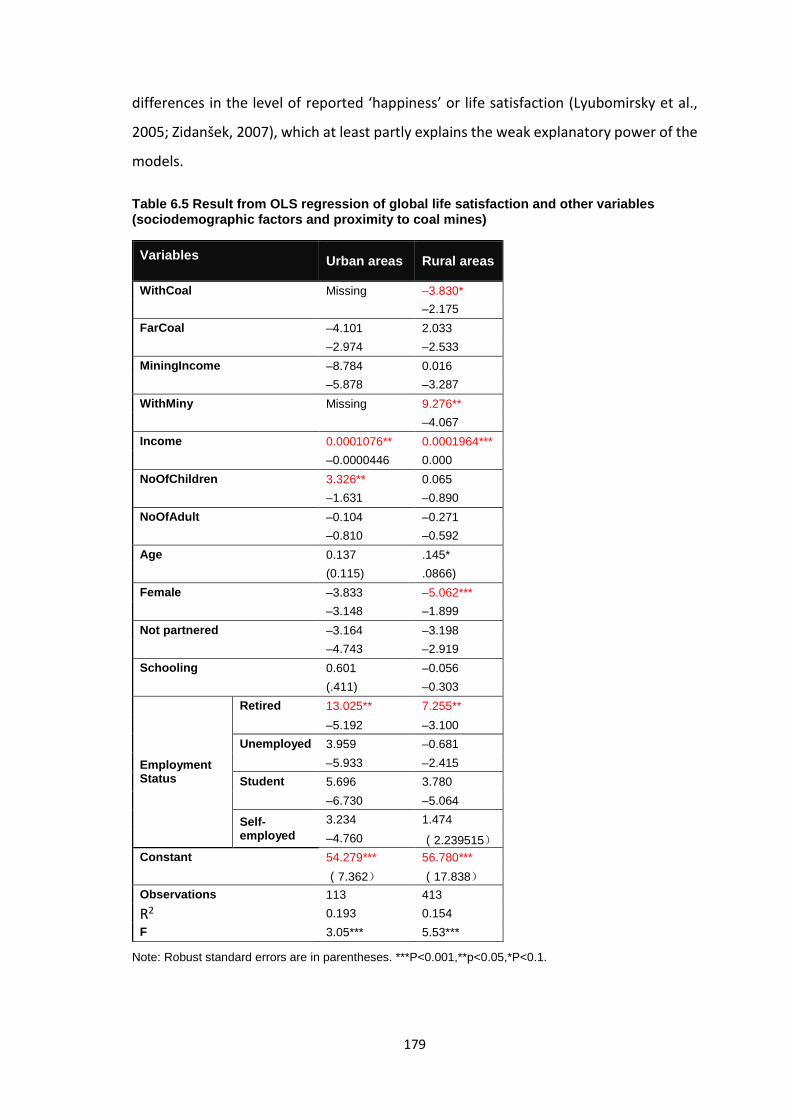
179

differences in the level of reported ‘happiness’ or life satisfaction (Lyubomirsky et al.,

2005; Zidanšek, 2007), which at least partly explains the weak explanatory power of the

models.

Table 6.5 Result from OLS regression of global life satisfaction and other variables (sociodemographic factors and proximity to coal mines)

Variables Urban areas Rural areas

WithCoal Missing –3.830* –2.175 FarCoal –4.101 2.033 –2.974 –2.533 MiningIncome –8.784 0.016 –5.878 –3.287 WithMiny Missing 9.276** –4.067 Income 0.0001076** 0.0001964*** –0.0000446 0.000 NoOfChildren 3.326** 0.065 –1.631 –0.890 NoOfAdult –0.104 –0.271 –0.810 –0.592 Age 0.137 .145* (0.115) .0866) Female –3.833 –5.062*** –3.148 –1.899 Not partnered –3.164 –3.198 –4.743 –2.919 Schooling 0.601 –0.056 (.411) –0.303

Employment Status

Retired 13.025** 7.255** –5.192 –3.100 Unemployed 3.959 –0.681 –5.933 –2.415 Student 5.696 3.780 –6.730 –5.064

Self-employed

3.234 1.474 –4.760 （2.239515）

Constant 54.279*** 56.780*** （7.362）（17.838） Observations 113 413 R2 0.193 0.154 F 3.05*** 5.53***

Note: Robust standard errors are in parentheses. ***P<0.001,**p<0.05,*P<0.1.

180

The effect of sociodemographic variables on GLS is generally consistent with those

identified in the models of domain-specific satisfaction. Income is a significant positive

contributor to global life satisfaction in both urban and rural areas. Retired people were

more satisfied with their life than others – even those of similar age and income. Age

was only positively significant in rural areas. People with more kids have higher levels of

satisfaction than other people in urban areas. Females were less satisfied with life

overall than males in rural areas.

After controlling for these sociodemographic differences it is possible to consider the

impact of mining. In urban areas, there were no statistically significant difference in GLS

between those who live close to or far from coal mining. Similarly, there were no

differences in GLS between those dependent on mining and other industries for

household income.

In contrast, in rural areas, people living in places with coal mining were less satisfied

with life overall than those living in places further away from coal mines (both ‘close to’,

or ‘far away’) (The difference between WithCoal and FarCoal is from post-estimation:

WithCoal minus FarCoal, Coefficient= –5.863, P=0.029). Noticeably, people living

adjacent to coal mines who were dependent upon coal mining for their income, had

higher reported levels of GLS than those who were not dependent upon coal mining

(even when both groups earned the same amount of income).

In both models the constants were statistically significant. However, post-estimation

comparisons of these coefficients reveal that there is no statistically significant

difference between them. This suggests that the variables included in the models are

able to explain systematic differences in GLS between Urban Close and Rural Close – i.e.

systematic differences are largely attributable to things such as age, retirement status,

income, and proximity to mining.

6.3.2.3 Assessing the economic ‘value’ (cost) of mining on GLS

• The amount of income that would need to be paid to ‘compensate’ someone

who had previously lived ‘near coal’, but then found themselves ‘with coal’ was

calculated as:

181

MRS=–𝜕𝜕𝜕𝜕𝜕𝜕𝜕𝜕/𝜕𝜕𝜕𝜕𝜕𝜕𝜕𝜕ℎ𝐶𝐶𝐶𝐶𝐶𝐶𝐶𝐶𝜕𝜕𝜕𝜕𝜕𝜕𝜕𝜕/𝜕𝜕𝜕𝜕𝜕𝜕𝐶𝐶𝜕𝜕𝜕𝜕

=–𝜕𝜕𝜕𝜕𝜕𝜕𝜕𝜕ℎ𝐶𝐶𝐶𝐶𝐶𝐶𝐶𝐶𝜕𝜕𝜕𝜕𝜕𝜕𝜕𝜕𝐶𝐶𝜕𝜕𝜕𝜕

= 3.830 / 0.0001964 ≈ 20,000

• The amount of income that would could be taken away from people (similar to

a ‘negative compensation’) who previously lived ‘near coal’, but then found

themselves ‘far from coal’ is assumed approximately equal to zero, since the

coefficient on ‘Far Coal’ is statistically insignificant.

It is interesting to note the statistical significance of the coefficient on the dummy

variable ‘WithMiny’. This suggests that in rural areas, those who are dependent upon

mining for income have higher GLS than people dependent upon other industries (say,

agriculture). If one wanted to raise the GLS of other people to the same level as those

working in the mining industry, then one would need to ‘compensate’ them with extra

income, the amount of which can be calculated as:

MRS=–𝜕𝜕𝜕𝜕𝜕𝜕𝜕𝜕/𝜕𝜕𝜕𝜕𝜕𝜕𝜕𝜕ℎ𝜕𝜕𝜕𝜕𝜕𝜕𝑀𝑀𝜕𝜕𝜕𝜕𝜕𝜕𝜕𝜕/𝜕𝜕𝜕𝜕𝜕𝜕𝜕𝜕𝐶𝐶𝜕𝜕𝜕𝜕

=–𝜕𝜕𝜕𝜕𝜕𝜕𝜕𝜕ℎ𝑀𝑀𝜕𝜕𝜕𝜕𝑀𝑀𝜕𝜕𝜕𝜕𝜕𝜕𝜕𝜕𝐶𝐶𝜕𝜕𝜕𝜕

= 9.276 / 0.0001964 ≈ 47,000

Whether this difference reflects the fact that people who work in the mining industry

(perhaps, having migrated from another region (see footnote 19, p. 163 )) are inherently

‘happier’ than those who do not, or whether the presence of a mine reduces the GLS of

people who are trying to earn a living in other sectors, cannot be determined from these

data.


Income is a significant positive contributor to some life domains and global life

satisfaction no matter whether in urban or rural areas. That is consistent with findings

from much research undertaken in both developed (e.g. Van Praag and Baarsma, 2005;

Welsch, 2006, 2008; Luechinger, 2009; MacKerron and Mourato, 2009) and developing

countries (Arifwidodo and Perera, 2011), and particularly with wellbeing studies

undertaken in urban China (Smyth et al., 2011). Knight et al. (2009) found out that

increases in the absolute level of income has a relatively weak impact on wellbeing in

rural China – what matters most is the impact that relative income has. The data in that

182

study were inter-province in 2002. It might be different after 14 years, and at different

scales of data (in this case, village/city level in one province).

The results associated with the other sociodemographic factors, such as age, are

generally also consistent with findings from previous studies. Notably, age has a positive

and significant impact on subjective assessments of satisfaction with several life

domains, such as the economy, social capital and living conditions, and also on GLS in

rural areas. As discussed in 2.2.3.5, other researchers have found that ‘middle aged’

people tend to have lower satisfaction with many factors than the young and old. The

finding here is probably in line with this, as the majority of respondents were over 35

years old (see Table 3.9) – suggesting that the sample for this study is (simplistically), on

the right hand side of the “U”– shaped relationship so frequently observed, thus

explaining the uniquely positive relationship.

Previous studies about the effect of having more children on wellbeing were mixed

(Dolan et al., 2008). The result reported here – that having more children can increase

life satisfaction – is consistent with those in the studies on subjective wellbeing in China

(Appleton and Song, 2008; Smyth et al., 2011).

Females were less satisfied with life than were males. Previous studies into the effect of

gender on wellbeing have published differing results. Some previous researchers have

found no gender differences for GLS (Travers and Richardson, 1993; Saunders, 1996),

some have found that women are generally happier than men (Clark and Oswald, 1996;

Hartog and Oosterbeek, 1998), but others (Hess et al., 2004; Stevenson and Wolfers,

2009) have found that men are happier. Subjective wellbeing studies undertaken in

urban China, in particular, found that man were less satisfied with their lives than

women (Russell et al., 2006; Appleton and Song, 2008). However, gender was not a

significant variable in the study about wellbeing in rural China (Knight et al., 2009), in

which data were collected at a provincial-level. Thus, based on the mixed evidence, it

might be thought that the gender effect on wellbeing is complicated, which might

depend on the cultural factors, geographic areas the data covered, in terms of urban

and rural areas, the administration level in terms of inter-province or single province, or

even the type of wellbeing measure (Smyth et al., 2011).

183

People with higher education level reported lower levels of satisfaction with their living

conditions and with the environment than others. This might be explained by the fact

that highly educated people have higher expectations which lowers reported levels of

satisfaction (Clark and Oswald 1996; Arifwidodo and Perera, 2011).

That coal mining had impacts on satisfaction with various life domains (even after

controlling for confounding factors) was clearly illustrated in this study: reported

satisfaction with the natural environment and the economy were significantly lower in

rural coal mining areas (Rural With and Rural Close) than in areas disassociated from

mining (Rural Far). Satisfaction with human capital, social capital and institutional capital

in coal mining areas (either Rural With or Rural Close) also tended to be lower than in

rural areas far from coal mining. In contrast, rural residents living far away from mines

were generally less satisfied with their living conditions than others. In urban areas,

residents living a long way away from mines were more satisfied with the natural

environment and institutional capital than those near mines. The consistency between

these results and the findings of other researchers is discussed below.

Satisfaction with the natural environment (overall air quality, air cleanliness, dust and

water safety) varies obviously with distance from coal mines, reflecting the significant

impact of coal mining on the environment which has been documented in a large

number of studies (e.g. Szczepanska and Twardowska, 1999; Ghose and Majee, 2000;

Tiwary, 2001; Bian et al., 2010). The concern with environment is often related to the

concern with health (Mackerron and Mourato, 2008). That coal mining had a negative

impact on human capital found in this study is also well documented in the literature

(Bian et al., 2010; Zullig and Hendryx, 2010, 2011; Colagiuri et al., 2012).

Although coal mining is said to be a significant contributor to the local economy (Editor

of Land & Resource Herald, 2013), people were less satisfied with the economy in rural

coal mining areas than in the non-coal mining areas. Notably, in this study the economic

domain not only includes satisfaction with income, it also captures (satisfaction with)

the inflation rate, the price of necessities, real estate prices, income disparities, and

fairness/equity. The message from chapter 5, highlights that actual family incomes and

satisfaction with income do not seem to be higher (or lower) in mining areas, so

184

dissatisfaction with the economic domain likely reflects dissatisfaction with other

economic factors.

The observed dissatisfaction with the economy in rural coal mining areas might thus be

explained by the following dynamic. Within coal mining regions, the economy is

supported by coal mining, but this drives up living costs (Carrington et al., 2011) and

creates a significant income gap between those dependent upon the coal mining

industry and those dependent on other industries (see Table 3.9, Appendix B, and

(Carrington et al., 2011)). Local residents who are not able to share the resource rent

become relatively worse off (Xu and Wang, 2006; Zhang et al., 2008; Zhao and Liu, 2011).

This is consistent with a survey undertaken by the CSIRO, which highlighted the fact that

benefits from mining in China were not distributed fairly, and that people living in mining

regions strongly believed that incomes were less equitable in their area as a

consequence of mining than those living in non-mining areas (Zhang et al., 2015). These

issues are also similar to what happened in other countries (Carrington et al., 2011). As

the proportion of population who had jobs from coal mining was relatively small in any

area (see Table 3.9), the level of global life satisfaction and satisfaction with the

economy were still lower in the places with higher intensities of coal mining.

Interestingly, the statistical significance of the dummy variable ‘WithMiny’ indicates that

resentment between mining and non-mining sectors may go beyond observed income

differences (the regression controls for those differences, but still finds evidence to

suggest that those not associated with the mining industry were disaffected).

This study also found evidence of the negative impacts of coal mining on social capital

(honesty, help, trust, personal relationships and personal safety), which is consistent

with the findings of other studies (e.g. OECD, 2001; Kitula, 2006; Lockie et al., 2009;

Carrington et al., 2011). The uneven distribution of benefits from coal mining, the issues

over the amount of compensation from coal mining, and the competition over mining

jobs, induced conflict and mistrust in the coal mining area. Although this study did not

collect data from the mining companies, anecdotal evidence (collected during

conversations with residents of villages) suggests that on average, only about 30% of

coal miners are ‘local’ residents; most workers are imported, by companies, from other

185

regions. The reliance on a large non-resident workforce, who had no meaningful

attachment to community, might disrupt existing social bonds and networks leading to

a loss of community identity and personal security (Carrington et al., 2011).

This study found that coal mining also affected institutional capital in some regions

(Urban close and Rural Close), which is consistent with the findings of many other

studies (e.g. Marshall, 2001; Sachs and Warner, 2001; Petermann et al., 2007). Evident

from those studies, if the governance is poor and fails to avert the dangers that

accompany the free gifts of nature, natural-resource-rich economies breed socially

damaging rent-seeking behaviour and corruption.

In contrast, it seems that mining is positively associated with better living conditions,

(which capture factors such as water supply, electricity supply, property safety and

quality of housing). This was the only domain that people living in places with coal

mining and near to coal mining were more satisfied with than those living far from coal

mining. This is consistent with the message from the objective indicators presented in

chapter 5, which showed that the percentage of houses with bathrooms and flushing

toilets in coal mining areas was larger than that in non-coal mining areas. The survey by

CRISO in China also highlighted the perceived improvements in infrastructure by

residents living in mining areas in China (Zhang et al., 2015).

The impacts of coal mining on life domains is thus demonstratively complicated, with

negative impacts on multiple domains and positive impacts on living conditions. As

discussed in chapter 2, in normal circumstances, it would be exceedingly difficult to

discern a ‘net impact’, without undertaking several non-market valuation studies,

seeking to monetise the value of the non-market impacts associated with the

environment, and with social and institutional capital. The global life satisfaction model,

however, allows one to consider the net overall impact of all effects.

After controlling for sociodemographic and ‘mining proximity’ factors, there were no

significant differences between urban and rural areas in terms of global life satisfaction

(a subjective measure). This is in spite of the apparently ‘obvious’ gap in objective

wellbeing indicators between urban and rural areas (e.g. fewer houses with bathroom

and toilets in rural areas) highlighted in chapter 5. This confirms insights from previous

186

chapters that objective measures alone, do not provide information about how satisfied

people are with their life. This difference between subjective and objective assessments

is consistent with the findings of Davey et al. (2009), who conducted a door-to-door and

street survey in both an urban area and a farming community (using PWI), finding similar

subjective wellbeing levels in both regions. This finding was, despite significant

differences in objective indicators. This may be partly explained by recent improvements

in lifestyle in rural areas – respondents may compare today’s situation (when they feel

there is ‘enough’ to satisfy their needs) with their past (when they were in poverty),

concluding that life is, indeed better now than it has been and thus feeling relatively

satisfied (Davey, Chen et al., 2009; Davey and Rato, 2012). Anecdotal evidence also

suggests that there have been more marked improvements in rural lifestyles of late,

than in urban lifestyles, perhaps also explaining why rural respondents’ outlook on life

overall is similar to that of urban residents, despite the vast gap revealed by objective

indicators in this study .

When GLS was compared across different regions without controlling for confounding

sociodemographic variables (such as age, gender) it seemed as if there were no

differences associated with coal mining. However, when sociodemographic factors were

controlled for (within the regressions), the statistically significant impact of mining

became apparent: rural residents living in areas with higher intensities of coal mining

had lower levels of life satisfaction than do those living more than 10km away from coal

mining. Living in the places with coal mining is equivalent, in life satisfaction terms, to a

drop of about 20,000 Yuan in annual family income compared to people living near coal

mining.

What also seems to matter is whether rural residents obtain a direct benefit from coal

mining or not: those who lived in places with coal mining and who were dependent

upon coal mining for their household income, reported significantly higher levels of life

satisfaction than those who were dependent upon other industries for their living. This

difference in life satisfaction is equivalent to a difference in income of 47,000 Yuan.

In contrast, there was no significant difference in GLS between urban residents living

close and far from coal mining. Since there was no difference in GLS between rural

187

residents living close to coal mines and far from coal mines either, it might be inferred

that close proximity to coal mines is a decisive contributor to GLS – only people living

very close to the mines (in this case, Rural With) were affected. There was statistical

difference in the satisfaction with the natural environment and institutional capital

between urban areas close to coal mines and far from coal mines, but there were no

significant difference in satisfaction with any other domain between these 2 groups.

Rural residents near coal mines, in contrast, were more dissatisfied with multiple life

domains than those living far from coal mines (the environment, the economy, the

institutional capital and human capital), but more satisfied with living conditions than

those living far from coal mines. Thus, apart from distance, urban areas might be

relatively insensitive to the impacts of coal mining, confirming the suggestion from

section 4.4. The potential reason for this was also discussed in that section.

The core issue for coal mining areas revealed by this chapter is that there is an uneven

distribution of benefits and costs from coal mining, both at a reginal level and individual

level. At the regional level, the nature of mining itself tends to breed this inequity local

communities in coal mining areas tend to bear most of the environmental and other

social costs associated with mining (as confirmed in this study by the negative impacts

of coal mining on satisfaction with those life domains), while the benefit flows largely to

the central government and elsewhere (Davis and Tilton, 2005). The host communities

get little from mining besides monetary benefits flowing from corporate taxation and

royalties (Zhao and Liu, 2011; Lei et al., 2013; Davis and Tilton, 2005), which might be

used to improve living conditions in this case. This further explains that residents living

in areas with higher intensities of coal mining have lower life satisfaction levels, after

controlling for other factors.

At individual level, people whose family income were dependent on coal mining were

the ones who benefited from coal mining, and experienced higher level of GLS than

those whose income were not dependent on coal mining. Data collected in this study

indicate that the proportion of respondents whose households were dependent upon

the mines for income were 32.%, 16% 15%, respectively in Rural with, Rural close, and

Urban close (see Table 3.9). As noted above, most workers (approximately 70%) are

imported by companies from other regions. Those non-residents workers may lack

188

attachment to local communities (Carrington et al., 2011), the negative impacts of coal

mining on the local environment and community may thus not be as much of a concern

to them as it is for permanent residents with attachment to affected places and people.

The differences might also at least partially reflect the fact that those who were working

in other industries (e.g. agriculture), might experience damages that directly impinge

upon their lifestyle and thus affect their wellbeing even it has little impact on income.

The interviewees’ concern with the impacts on coal mining on their livestock and

farmland demonstrate this (see the quotes in p. 124 and p. 125).

Other studies of the resource curse in Shanxi province confirm that coal resource

development tends to impede economic growth. Xu and Wang (2005), for example,

used data at the province level, and Fu and Wang (2010) used data at the city level,

empirically testing the “resource curse” hypothesis and finding evidence to support it in

Shanxi Province. This study, using subjective wellbeing data collected at the individual

level, not only finds that mining does not seem to have an unambiguous and positive

impact on incomes in Shanxi Province (which is consistent with previous studies on the

resource curse), but has also furthered the understanding of the potential negative

consequences of mining to other domains, such as environmental and social domains.

As discussed in section 2.4, uneconomic growth occurs when the marginal disutility of

an activity (here, the negative impacts of coal mining) outweigh its marginal utility (here,

the positive impacts of coal mining). This study found a net negative impact of coal

mining on GLS, which could also be inferred from strong negative impacts of coal mining

on multiple environmental, economic and social domains, but positive impacts only on

living conditions. This might suggest that for those who participated in this study, coal

mining is an ‘uneconomic’ form of growth – at least for those in the rural areas with coal

mining.


This study highlights the fact that coal mining does not necessarily improve the

wellbeing of those living in host communities. On the contrary, coal mining had net costs

to people living in rural places with coal mining. This is revealed by the significantly lower

189

level of reported global life satisfaction for people who live with mining compared to

those who live further away. It is attributable to the negative impacts that mining has

on the environmental, social, and economic domains. Although coal mining did not

appear to generate net negative impacts to those living in Rural Close and Urban close

areas (might be because the negative impacts were not very strong or did not outweigh

the positive impacts), it did negatively impact the environment, economy, human capital

and institutional capital in those regions. The direct implications of this chapter for policy

makers to improve wellbeing in coal mining area (especially in Rural With) and the

problems associated with these strategies are discussed below.

• Relocation

Those living in places with coal mining who were not employed in the industry had

relatively low levels of overall life satisfaction and were less satisfied with multiple life

domains than other people. Relocating these people might thus improve their wellbeing.

Relocating entire villages is not common and very few instances of that were

encountered in this survey. Instead, it seems more common for individual houses to be

relocated – particularly if an individual’s land is to be used by the coal mining company.

Discussions undertaken with local residents while collecting data revealed that they do

not generally self-relocate, most likely because they are unwilling or unable to abandon

their houses and spend their own money building a new house somewhere else. Instead,

mining companies who need to access land, compensate people to encourage them to

move to other places (some even move to urban areas). The statistical analysis in this

study did not consider relocated individual or households, as they were dispersed in

different places.

Relocation may have improved the wellbeing of those who moved into better dwellings

than the ones they vacated. But such opportunities can create perverse incentives.

Some people, see the possibility that they could be relocated, and enlarge their existing

houses, or even adding a second or third floor – with the expectation of more

compensation (see Figure 6.6). This is a private form of ‘rent seeking’ – wasteful

expenditure of money (building a house that one knows will be knocked down) in an

attempt to gain still more money (see the definition of ‘rent-seeking’ by Henderson

190

(2008)). To the best of my knowledge, no one has empirically studied the extent of this

from of rent-seeking, which is different from the well-documented rent-seeking

behaviour usually conducted by governments (Marshall, 2001; Sachs and Warner, 2001;

Petermann et al., 2007; Wright, 2008).

Figure 6.6 Simple dwellings built to elicit compensation Source: Taken by the investigator in a village with coal mining on 25th August 2013

• Financial compensation

This study suggests that people living in places with coal mining, especially those unable

to obtain jobs from coal mining, could, potentially, be financially compensated. This

study also generated some estimates of the magnitude of compensation required, which

could be used as a straightforward reference for public policy. However, there are some

problems likely to arise should this option be considered.

It may be difficult to implement using existing compensation systems, characterized by

rent-seeking and corruption. This also at least partly explains the low level of satisfaction

with institutional and social capital in the coal mining areas. According to local residents,

in many cases, the financial compensation that coal companies paid to regions was

managed by local governments. Without enough transparency and supervision, self-

benefit-motivated government officers might be involved with rent–seeking behaviour;

a sensitive topic in the coal mining areas in China. In some coal mining villages, some

people were reluctant to be interviewed for this study especially when they were not

sure what questions would be asked about coal mining. However, they expressed openly,

191

sometimes indignantly, their opinion on matters relating to issues of monetary

compensation (see the quotes in p. 123).

When the head of one village answered the question about family income, another

respondent overheard his answer. He said to the investigator afterwards, “He is lying.

He is the richest person in this village, and owns a lot of real estate in the city, because

he got a lot money from the coal company. Anecdotally the investigator found that this

was not an extreme case: corruption associated with mining is an open secret in China,

and is also well discussed in the literature in other contexts (e.g. Marshall, 2001; Sachs

and Warner, 2001; Petermann et al., 2007). However, due to the obfuscating nature of

corruption, there is very little empirical evidence of actual levels of corruption in the

mining sector or its interaction with individuals and communities (Marshall, 2001).

These difficulties will remain (perhaps even be exacerbated) if formal compensation

programs include a broader range of impacts (such as those identified in this study) than

those normally considered (such as damage to the physical environment and direct

economic loss of local residents (e.g. loss of house/land or farmland, or the loss of

income that could have been generated from the land) (Zhao and Liu, 2011)).

Figure 6.7 Government building of Pinglu (a), and residential dwelling in a village with coal mining, administrated by the Pinglu government (b) Source: Photo ‘a’ was taken by the investigator in a city close to coal mines on 22th August 2013; Photo ‘b’ was taken by the investigator in a village with coal mining on 25th August 2013.

a b

192

A second fundamental problem with the idea of using LS studies to firstly estimate

required amount of compensation and then actually pay that compensation is that the

system itself, creates an incentive for (perverse) strategic behaviour on the part of those

involved in the survey. In this study, questions about satisfaction with life overall were

not linked to coal mining, and were asked before the questions about coal mining. In

addition, the interviewees were not aware that the data could, in principal, be used to

estimate financial compensation. Thus, there was no reason for respondents to answer

the life satisfaction questions strategically. However, if policy makers decided to use life-

satisfaction studies as a way of estimating compensation, and if people grew to expect

it, then they may cease responding honestly to questions contained within LS surveys –

instead responding strategically so as to maximise compensation (just as some behave

strategically when thinking they may receive compensation if asked to relocate).

Likewise, governments (or mining companies) might be given a strong incentive to

manipulate the subjective measurement in their favour (Frey and Gallus, 2013). Thus,

like relocation policies, compensation policies also have the potential to create perverse

incentives and caution must be exerted if considering using LS studies in this way.

• Delivering more jobs from coal companies

As mentioned above, anecdotal evidence, consistent with the survey data, suggests that

on average, only about 30% of coal miners were ‘local’ residents; most workers were

imported, by companies, from other regions. This suggests that the mines could

potentially, provide more jobs for ‘locals’.

Hiring non-residents workers is a common practice in the mining sector, not only in

China, but also in developing countries like Australia (Carrington et al. 2011). However,

the reason for coal companies hiring non-resident workers differs between China and

other countries. For sparsely populated countries, the difficulty of sourcing labour due

to the isolation of the mining sites, as well as short project life are the basic reasons for

the tendency of hiring non-residential workers (Gillies et al., 1991, cited by Carrington

et al. 2011, p. 338). In China, with a high density of population, it is not difficult to source

labour in most regions suggesting that there may be other reasons for this practice.

193

Anecdotal evidence collected during discussions with respondents when collecting data,

suggests that one of the reasons coal companies hire miners from other regions is

because of a perception that local residents are more ‘resilient’ and thus potentially less

easily controlled or manipulated. Local residents have more family and community

support, than miners brought in from elsewhere, and in the event of accidents or other

disputes, they tend to demand higher compensation and are able to hold out for longer

against the companies during negotiations. As such local residents may be more ‘costly’

and/or more ‘difficult’ to deal with than workers brought in from other areas. Anecdotal

evidence suggests that locals who manage to find jobs with coal companies are most

often those who have a strong personal relationship with the owner. That said, local

residents who manage to get jobs in the coal mining industry are likely to be allocated

the low-pay/low-risk jobs, rather than the high-pay/high-risk jobs given to outsiders.

As discussed in section 4.4, in one of the villages included in this study, a condition

imposed upon the coal company when it sought permission to start operating in the

region, was that it hired ‘locals’. Results from the regression analysis undertaken in this

chapter suggest that people who were dependent upon coal mines for household

income (and thus more intimately associated with them) had higher GLS than those

dependent upon other industries. So there is prime facie evidence to suggest that such

a strategy might improve the LS of residents. The evidence is not, however, conclusive:

it is possible that requiring (or suggesting) that people who are currently working in

agriculture may not want to work in mining – and would be even unhappier if forced to

change (although this line of reasoning presumes that people have alternatives: such

may not be the case).

That point aside, by providing more jobs to locals, the mine will have a more significant,

positive, impact on the local economy in terms of improving local residents’ income,

reducing income disparities and thus improving equity. Delivering more jobs means

allocating more benefits to people living in coal mining areas, which is an important

pathway to compensate people experiencing the negative side effects of coal mining.

Additionally, hiring more local residents could help maintain and improve social capital.

It can reduce the factors that induce conflict and mistrust in the host communities

resulting from the uneven distribution of benefits and costs, the competition over

194

mining jobs and the flow of a large amount of non-resident workforce into local

communities. As discussed in section 1.3.4, large numbers of non-resident workers

without meaningful attachment to the resident community can contribute to the

disruption of social capital (OECD, 2001; Kitula, 2006; Lockie et al., 2009, Carrington et

al., 2011), so a ‘hire local’ policy could help reduce those impacts. Notably, caution must

be exerted when delivering more jobs to local communities. Affirmative action policy,

which regulates the allocation of scarce positions in employment could possibly reduce

incentives for effort and skill acquisition in the targeted group (Fryer Jr and Loury, 2005).

Compared to the options of relocating residents or providing monetary compensation,

providing more mining jobs to locals seems a less costly strategy for coal mining

companies, whose training and salary costs are unlikely to be different for local and non-

local workers. However, delivery of more mining jobs from coal companies requires the

formulation of clear compensation standards and procedures which not only guarantee

local residents’ rights but also ease the coal companies’ concerns with the negotiation

power of locals. In reality, these strategies of relocation, money compensation and job

delivery might have to be combined or used accordingly under the supervision of

government with a transparent mechanism.


The effects of coal mining or mining in general may vary between districts or countries,

as it is a complicated issue that may involve government policies, the mining industry

management, or even historical and cultural factors. Notwithstanding, this chapter

further confirmed that subjective wellbeing data provide information about people’s

satisfaction with existing conditions in local communities, and can be used to

supplement objective wellbeing indicators that are traditionally used.

This study extends the research on coal mining or mining impact assessment by offering

a new tool to assess impacts associated with mining. As discussed in section 2.2.1.2, the

difficulty of simultaneously quantifying numerous intangible impacts using non-market

valuation techniques limits their application in traditional impact assessments. The LS

approach, with the capacity to compare the impacts of mining, on wellbeing, of both

195

monetary and non-monetary impacts, allows for a more comprehensive assessment of

the trade-offs associated with mining (indeed with any) industry, and can thus offer

policy makers a straightforward reference to determine whether a project is economic

or non-economic. If it is non-economic (in that a net cost (on GLS) is likely to occur), the

monetary net cost can be used as a reference for compensation for those impacted

groups. The LS approach can also allow one to identify differences in impacts (be they

positive or negative) between different groups (in this study, impacts between those

who were, or were not, dependent on the mining industry for their livelihood were

compared), again, in monetary values, and to adjust compensation amounts accordingly.

Therefore, the LS approach, offering different insights into communities’ preferences,

can be used as a complementary tool for a range of other traditional approaches of

mining assessment (Ivanova et al., 2007). Alternatively, the LS approach could be

incorporated into the cost benefit analysis (CBA) framework and used instead of other

techniques (such as choice modelling (e.g. Gillespie and Kragt, 2010)) to capture, and to

measure a wide variety of non-market impacts, such as those associated with air

pollution (Welsch, 2006; Luechinger, 2009b; MacKerron and Mourato, 2009).


The dummy variables relating to coal mining were not significant for urban samples in

terms of GLS and satisfaction with most domains, which might be because urban

residents are less vulnerable and thus less sensitive to the impacts of coal mining than

rural residents (see section 4.4 and earlier this section). However, the lack of statistical

significance may reflect the fact that the urban sample was relatively small. Future

research, working with larger samples, could shed light on this important issue.

Also, Knight et al. (2009) found out that increases in the absolute level of an individual’s

income has a relatively weak impact on wellbeing in rural China: what increases

satisfaction most, is an increase in income relative to others. Future studies could also

thus usefully expand this research by considering relative income in the LS models.

Endogeneity may also be an issue that future studies could consider, and thus improve

upon the techniques demonstrated here. Endogeneity of income is a common problem

196

in the LS literature (e.g. MacKerron and Mourato, 2009; Ferreira and Moro, 2010;

Pischke, 2011). It occurs because income depends on many factors such as working

hours, stress, health risks, etc. that also impact LS and which are difficult to control for

(Ferreira and Moro, 2010). Omission of such factors induces downward bias in the

income estimates, which could result in an upward bias in these estimates of

‘compensation’ (Ferreira and Moro, 2010). That said, some researchers (e.g. Pischke,

2011) have used instrumental variables to control for endogeneity, finding that results

do not differ much between models that do, and do not control for endogeneity. As this

study did not control for endogeneity issues, estimates of compensation are only

illustrative and may not be accurate. When using as a guide for policy makers, future

studies with more sophisticated econometrics to control for this issue may need to

generate monetary values with more confidence.

197

Thesis outline

198

7. CHAPTER 7 SYNTHESIS AND DISCUSSION

Chapter outline

7.1 Introduction

7.2 Overview of the thesis

7.3 Empirical contributions

7.4 Discussion of empirical findings

7.5 Methodological contributions and implications for policy makers or practitioners

7.5.1 Methodological contributions and insights for monitoring / measuring wellbeing

7.5.2 Methodological contributions to the impact assessment literature

7.6 Implications for future research

7.7 Concluding comments

199

7.1 Introduction

This chapter first reviews key parts of the thesis and presents clear answers for each of

the core research questions addressed in the 3 main data/analysis chapters (section 7.2).

Key findings are synthesized in section 7.3 – highlighting the main empirical

contributions of the thesis. Section 7.4 discusses empirical results within the context of

the broader literature. The methodological contributions of this research and

implications for policy makers or practitioners are discussed in section 7.5, whilst section

7.6 highlights key areas in need of future research.

7.2 Overview of the thesis

Coal has played a vital role in human history. Threats of anthropogenic climate change

associated with coal use have become a concern, and have given rise to demands for

cleaner, renewable fuels. Nevertheless, for decades to come, coal use will likely continue

to grow, mostly driven by growth in the developing world (International Energy Agency,

2010). Coal, as the most affordable and widely available source of energy is of particular

importance to poor regions with abundant coal resources: coal does not only generates

affordable energy, which is essential for economic growth, eliminating poverty and

improving wellbeing (Cousins, 1998; Karekezi, 2002; Pachauri and Spreng, 2004;

Kammen and Kirubi, 2008), but coal mining and processing also directly promotes

regional development and wellbeing by delivering jobs, and tax revenues for

government to fund infrastructure improvements.

Benefits aside, host communities are most exposed to the negative impacts of coal

mining, with the industry affecting natural capital (e.g. land, water and air (Bian et al.,

2010; Colagiuri et al., 2012)), human capital (e.g. education (Gylfason, 2001), health

(Bian et al., 2010; Zullig and Hendryx, 2010, 2011; Colagiuri et al., 2012)), social capital

(e.g. trust, social injustice (Kitula, 2006; Carrington et al., 2011)), institutional capital (e.g.

promoting rent seeking and corruption (Marshall, 2001; Sachs and Warner, 2001;

Petermann et al., 2007)), and the broader economy (e.g. increasing prices (Colagiuri et

al., 2012)). But coal is rarely mined to meet only the needs of local residents; rather it is

transported to other regions to support the economy of the whole nation. A core

200

question thus becomes: how does coal mining affect wellbeing in host communities, i.e.

to what extent does the host community benefit from coal mining, considering all of the

above?

This question, essentially, is about the incidence and distribution of benefits and costs.

It receives relatively little attention – by either researchers or by policy-makers/advisors.

One reason for this is that current methodological approaches designed to inform

comprehensive assessments struggle to fully account for, and provide quantitative

information about such a broad and diverse range of impacts as those associated with

coal mining.

There are numerous existing frameworks for assessing the impacts of mining, such as

environmental impact assessment (EIA), social impact assessment (SIA), and economic

impact assessment (e.g. cost benefit analysis (CBA)) which have been used with varying

success in multiple contexts (e.g. Joyce and MacFarlane, 2001; Ivanova et al., 2007; Li,

2008). In theory, a comprehensive impact study would consider all impacts. Some

frameworks (specifically, CBA) even allow one to generate estimates of ‘net impact’. This

is done by firstly identifying ‘impacts’ and then using both market and non-market

valuation techniques to generate monetary estimates of the ‘value’ of all impacts,

including those relating to environmental degradation), which can be added, or

subtracted from other financial estimates to calculate ‘net benefit’.

Established methods for generating monetary estimates of the ‘value’ of non-market

impacts include revealed preference (RP) and stated preference (SP) approaches – with

a relatively long history (and almost 50 years of research to support them). Hedonic

pricing (one of several different RP methods) and choice modelling (a type of SP method)

have been used in mining impact assessments (Trigg and Dubourg, 1993; Ivanova et al.,

2007; Gillespie and Kragt, 2010), but these studies most often consider only a limited

number of non-market impacts – almost certainly because of the technical difficulties

(and thus resource costs) of generating estimates of non-market impacts. Moreover, RP

and SP approaches require one to assume that respondents are ‘rational’, have full

(perfect) information, and that markets are in equilibrium (Welsch, 2006). As such,

existing methods for assessing impacts of mining are limited in their ability to

201

simultaneously quantify numerous impacts on values that are not amenable to non-

market and to thus assess potential trade-offs between the costs and benefits of mining,

properly taking into account the welfare of host communities (Ivanova et al., 2007).

This study aimed to address those issues by asking – from the perspective of residents

of host communities – whether the positive aspects of coal mining outweigh the

negative. Identifying trade-offs between positive and negative impacts, provides a policy

reference, which can be used to address impacts of mining thus maintaining, and

potentially even improve local wellbeing.

Life satisfaction is considered to be one of the dimensions of wellbeing, although

sometimes the phrase is used interchangeably with ‘wellbeing’ (see section 2.3). Coal

mining has the potential to impact numerous factors that contribute to wellbeing, so

this study looked beyond just LS, investigating the impacts of coal mining on overall life

satisfaction and on numerous factors (and domains) known to influence wellbeing.

This fills important knowledge gaps: not only does previous research lack

comprehensive assessments of a large number of the benefits and costs of coal mining

(individually, or ‘in aggregate’), but it also lacks research that provides insights about the

utility of subjective (as opposed to objective) indicators of wellbeing. Most previous

research has used objective indicators of wellbeing – such as income – when assessing

impacts. But there may be instances when objective indicators are unavailable (almost

always when considering indicators of social capital) or inadequate (consider a region-

wide measure of average annual rainfall that fails to capture differences in rainfall within

the region). Previous research lacks examples of investigations that use subjective

indicators of wellbeing; examples of studies could not be found that explore the

relationship between objective and subjective indicators, and/or that provides guidance

about situations in which it is ‘better’ to use objective or subjective indicators when

assessing ‘impacts’.

This thesis thus collected data on, and tested the efficacy of several types of subjective

indicators: specifically, the perceptions of local residents of the importance of wellbeing

factors to their overall wellbeing, their satisfaction with those factors, and their

perceptions about the way in which coal mining affects those factors. The relationship

202

between those indicators, and between subjective and objective indicators was also

explored, thus providing information to fill important gaps in our understanding of the

ways in which to measure and monitor wellbeing.

The LS approach was then used to assess net benefit. It is a relatively new method, which,

unlike other non-market valuation approaches, does not require one to assume

rationality, or equilibrium; neither does it evoke strategic behaviour (Welsch, 2006). It

has been used to assess the ‘value’ of a wide range of non-market goods (e.g. air

pollution (Welsch, 2006; Luechinger, 2009; MacKerron and Mourato, 2009), airport

noise (Van Praag and Baarsma, 2005), corruption (Welsch, 2008)), but is has never been

used in mining contexts. Therefore, this study adopted the LS approach to measure the

net impact of coal mining on LS and on satisfaction with various life domains. The thesis

thus does more than just assess net impact; it also provides comprehensive information

about the impact of mining on a broad range of factors known to influence wellbeing,

and in doing so, demonstrates a new method for considering mining (or other) ‘impacts’.

Shanxi Province in China was selected as the case-study area. Data were collected from

places with different intensities of coal mining, including rural areas with coal mining

(Rural With), rural areas close to coal mining (Rural Close), urban areas close to coal

mining (Urban Close), urban areas far from coal mining (Urban Far) and rural areas far

from coal mining (Rural Far). This sampling strategy was chosen to enable cross-regional

comparisons that allow for insights which could not be gleaned if focusing only on, for

example, mining communities.

In total, 542 questionnaires were completed, providing information about people’s

global satisfaction with life (GLS), about their satisfaction with 29 factors known (from

the literature) to contribute to wellbeing, about their subjective assessment of the

importance of those factors to overall quality of life, and about the perceptions of the

impacts of mining on those factors. Background sociodemographic information (also

known to be associated with subjective assessments of wellbeing) was also collected.

203

Figure 7.1 provides a visual overview of the key research questions addressed, the

methods adopted and the answers for each research question. The discussion below,

provides more detailed ‘answers’ to core questions.

204

Figure 7.1 Overview of the thesis

205

1. The overarching question considered in Chapter 4 was: How does coal mining affect

people’s subjective perceptions of different wellbeing factors? This includes

satisfaction with different wellbeing factors, the importance attached to each factor,

and people’s perception about impacts of coal mining on these factors.

Sub-questions, and summarised ‘answers’ are as follows:

1.1. What factors are important to people’s lives? Do people’s perceptions of what

is important differ in places with different intensities of coal mining?

Health and relationships (with family and friends) were rated as the most

important wellbeing factors consistently across regions. For most factors, mean

importance scores do not vary dramatically across different types of case-study

regions. But residents living in rural coal mining regions attached significantly

greater importance to factors relating to air quality.

1.2. How satisfied are people with those factors? Does satisfaction with particular


Overall, respondents were most satisfied with factors relating to health and

relationships, which was consistent across regions. People living in coal mining

area were less satisfied with factors relating to air quality, water safety, inflation

and price of necessities than those living in non-coal mining areas. The factors

with which people living in coal mining areas were most dissatisfied related to

air quality and the economy; in non-coal mining areas, people were most

dissatisfied with factors relating to the economy while air quality was not a

concern.

1.3. How do people think coal mining affects various aspects (factors) of their life?



Overall, the perceived impacts of coal mining on most factors were negative,

among which the most concerning factors related to the natural environment

and health, which was also consistent across regions. Compared to people living

206

in coal mining regions, people living in non-coal mining regions seemed to

underestimate the negative impacts of coal mining while exaggerating the

potential positive impacts. In particular, residents living far from coal mining

believed that coal mining may bring higher income or help decrease income

disparities, while residents living in coal mining areas did not report any

obviously positive impact of coal mining on income; instead they reported a

negative impact on income disparity.

1.4. Are people satisfied with the factors that they attach great importance to? Can


importance – i.e. can we identify factors which people are very dissatisfied with

and attach great importance to?

The Index of Dis-Satisfaction (IDS), which combines satisfaction and importance

scores, reveals that in coal mining areas respondents were most dissatisfied with

and attached greatest importance to factors relating to the environment (air

quality and water safety) and the economy; factors relating to the environment

were not a major concern for respondents in non-coal mining areas.

1.5. Are the factors that people are dissatisfied/satisfied with negatively/positively

affected by coal mining? Can one identify policy priorities by combining

information about satisfaction and impact – i.e. can we identify factors which

people (either rightly or wrongly) ‘blame’ coal mining for impacting most

negatively?

The Index of Dis-Satisfaction and Negative Impacts (IDSNI), which combines

scores relating to satisfaction and perceptions of the impact of coal mining,

convey the message that factors relating to the natural environment (dust, air

quality, air cleanliness, water safety), and the economy (real estate prices and

inflation) were the factors of dissatisfaction where coal mining had negative

impacts.

207

2. The overarching question considered in Chapter 5 was: Does information about the

impacts of coal mining derived from subjective assessments of wellbeing convey the

same message about the impacts of coal mining as ‘objective’ measures of wellbeing?


2.1. Do the objective indicators suggest that there are differences in wellbeing

between (a) areas with different mining intensities; and (b) rural and urban

areas?

Objective indicators reveal that coal mining had a significant negative impact on

air quality (reflecting findings from the previous chapter relating to ‘satisfaction

with air quality’ in mining and non-mining region). It had a positive impact on

housing conditions (high percentages of households with a bathroom and

flushing toilet). Coal mining had no obvious impact on family income (there were

no statistically significant differences in family income across mining and non-

mining regions, reflecting findings from the previous chapter which found no

difference in ‘satisfaction with income’ across those regions). Coal mining had no

obvious relationship with education. Family income, housing conditions and

education levels, were all significantly better/higher in the urban study areas

than in the rural study areas.

2.2. Do objective and subjective indicators convey similar information when (a)

using aggregated data and (b) using regressions at individual level to control

sociodemographic factors?

Both regional level data and individual data (analysed using regression to control

for confounding sociodemographic factors) reveal that higher levels of actual

family income were associated with higher levels of satisfaction with income,

and that higher levels of PM10 were associated with lower levels of satisfaction

with air quality. However, the objective indicators of housing selected in this

study were not always good predictors of subjective assessments of satisfaction

with housing, and there was no apparent relationship at all between the

‘objective’ indicator for education that was used here (the proportion of

208

respondents who have completed a certain level of schooling) and satisfaction

with education quality and opportunity. In all cases, when using regression, the

relationship between objective and subjective indicators was mediated by


3. The overarching question considered in Chapter 6 was: Is it possible to quantify the

net impacts of coal mining (on broad ‘domains’ of life and on the overall wellbeing

of host communities) and to determine how much should, in principle, be paid ‘in

compensation’ to those who are, overall, impacted negatively?


3.1. How does coal mining affect satisfaction with life domains (after controlling for


Urban residents living close to coal mining were generally less satisfied with their

environment and with institutional capital than urban residents living far from

coal mining. In rural areas, those living in close proximity to mines (both Rural

With and Rural Close) were less satisfied with the natural environment and the

economy, and those living in either with coal mines or close to coal mines

reported lower levels of satisfaction with social, institutional or human capital

than those living further away from coal mines. In contrast, rural residents living

in coal mining areas (Rural With and Rural Close) were more satisfied with their

living conditions than those living further away. The impact of coal mining on the

environmental domain seems to be more strongly negative than on any other

domain, and those living immediately adjacent to mines (the ‘Rural With’ sub-

sample) were even less satisfied with the environment than those living at least

10km away.

3.2. How does coal mining affect global life satisfaction (after controlling for


Residents in urban areas seem relatively unaffected by proximity to mines: after

controlling for sociodemographic factors, there was no statistically significant

209

difference in GLS between ‘Urban Close’ and ‘Urban Far’ sub samples. In rural areas,

residents of villages adjacent to coal mines were less satisfied with their life as a

whole than those living further away from mines (Rural Close and Rural Far).

However, the difference in GLS between Rural Close and Rural Far was not

statistically significant (after having controlled for sociodemographic). People living

in rural villages adjacent to mines who depended upon coal mines for their family

income were significantly more satisfied with their lives than those living in the same

region who were dependent upon other industries for their income.

3.3. If the net impact of mining, on global life satisfaction, is negative, then how

much extra income would need to be paid to the negatively impacted people,

to raise their ‘satisfaction’ to the same level as their unaffected counterparts?

Those living ‘with’ coal, would need to be compensated by 20,000 Yuan per

household per annum, to raise their GLS to a similar level as households who are less

affected by coal mines (those living close to, rather than ‘with’ coal mines). Those

who were dependent upon non-mining industries for a living would potentially need

to be ‘compensated’ 47,000 Yuan per household per annum, to raise their GLS to the

same level as those in similar regions who work in the coal mining industry.

7.3 Empirical contributions

The various metrics used in this thesis all suggest that the impact of coal mining on the

natural environment is most concerning. First, respondents perceived that coal mining

had strongest negative impacts on the factors relating to the environment than on other

wellbeing factors. Second, the objective indicator of air quality (PM10, measured in each

village in which data were collected) clearly showed that air quality was worse in regions

with or close to coal mines than in regions further away. Third, respondents who lived

in regions ‘with’ or close to coal mines were less satisfied with factors relating to the

environment than those living further away from mines – even after controlling

sociodemographic factors known to influence such perceptions in the LS models. Fourth,

the coefficient (from the models about satisfaction with different life domains in chapter

6) for the environmental domain is of higher magnitude than coefficients for other

210

domains, indicating that the impact of coal mining on the natural environment is

stronger than any other impact. This is consistent with the message from the Index of

Dis-Satisfaction (IDS) and the Index of Dis-Satisfaction and Negative Impacts (IDSNI),

which indicate that environmental issues were paramount coal mining areas.

Coal mining did not have a positive impact on average income; but had a negative overall

impact on the local economy. First, respondents from all areas believed that coal mining

had negative impacts on the inflation rate, real estate prices, and price of necessities;

respondents who lived with or near coal mines did not think coal mining had obviously

positive impacts on their income (although those who lived far away felt that coal mines

might improve their income). Second, objective indicator of income confirmed that

there was no significant difference in the household income between those living with,

near, or far from coal mines. Third, respondents from coal mining areas were not more

satisfied with their income or with other factors associated with the economy. After

controlling sociodemographic factors, coal mining was shown to have a negative impact

on the economic domain.

Objective indicators were not available for factors relating to social and institutional

capital. But subjective indicators suggested that coal mining might also have negative

impacts on these domains; perhaps even on human capital. Qualitative evidence

supported a link between the deterioration of institutional capital/social capital in coal

mining areas, although statistical results were not always significant for all the coal

mining areas (Urban Close, Rural With, Rural Close).

The only domain that coal mining had a demonstratively positive impact upon was that

of living conditions. This was ascertained by objective indicators (the percentage of

houses with bathrooms and flushing toilets in different case-study areas), and the high

levels of reported satisfaction with living conditions after controlling for


For the sample considered here, it is thus clear that coal mining generated negative

impacts on multiple life domains in rural coal mining areas (Rural With and Rural Close);

it only generated positive impacts within 1 domain (living conditions). For those living

‘with’ coal, the negatives outweigh the benefits, confirmed when analysing global life

211

satisfaction (GLS). The net negative impacts were equivalent, in life satisfaction terms,

to a drop of 20,000 Yuan in annual family income. In other words, this suggests that

those living ‘with’ coal, would need to be compensated by 20,000 Yuan per household

per annum, to raise their GLS to a similar level as households who were less affected by

coal mines (those living close to, rather than ‘with’ coal mines). Those who were

dependent upon non-mining industries for a living (e.g. agriculture) were even less

satisfied with life overall, compared to those who worked in the mining industry. They

would potentially need to be ‘compensated’ 47,000 Yuan per household per annum, to

raise their GLS to the same level as those in similar regions who work in the coal mining

industry. For rural areas and urban areas ‘close’ to coal mines, the negative impacts were

apparent, but might not outweigh the positive (living conditions), as the GLS was

statistically similar to those living far from coal mines, after controlling for confounding

factors.

Other studies also found net negative impacts of coal mining in other places. For

example, Hendryx and Ahern (2009) assessed negative impacts of coal mining on public

health (using value of statistical life (VSL)) relative to the economic benefits of the coal

mining industry in Appalachia region in USA, and found out the VSL costs outweighed

the economic benefit from coal mining. Bai et al. (2011) found a monetary net cost of

coal mining in Mentougou district of Beijing, using a CBA which estimated the economic

benefit (output value of coal), social benefit (employment opportunity, annual per

capita income and public infrastructure) and damage to water eco-service. Li et al. (2011)

also found the ecological and environmental loss caused by coal mining was far more

than its economic benefits in Mentougou district of Beijing.

However, these studies, like many other studies, use mainly market-based approaches

to calculate the costs and benefits of coal mining. Thus they can only involve a narrow

range of impacts, which could be easily linked to the market good, but very often

exclude other intangible/non-market impacts. As discussed in chapter 1, coal mining has

impacts on multiple life domains, so a defensible estimation of net impact should take

into account a wide range of impacts. This highlights the need to comprehensively assess

non-markets impacts on host communities in future mining impact assessments. Using

life satisfaction (rather than money) as a metric, this study provides a comprehensive

212

set of results which can be used to inform policy initiatives to address the negative

impacts of coal mining. Specifically, the results indicate that multiple life domains are

adversely affected (including those relating to the environment, the economy, or even

institutional capital, social capital and human capital); policy makers could seek to

explicitly redress those impacts, thus maintaining, or perhaps even improving the

wellbeing of those in host communities by, for example, providing more housing (to ease

pressure on real-estate prices) and/or ensuring that ‘locals’ have the opportunity to

work in the mines (rather than importing workers from outside the region).

7.4 Discussion of empirical findings

This study highlights the fact that coal mining does not necessarily improve the

wellbeing of those living in host communities. On the contrary, it brings net costs to

people living in rural places with coal mining areas, consistent with studies that involved

much less domains (Hendryx and Ahern, 2009; Bai et al., 2011). Key findings from this

study, regarding the life domains likely to be positively and negatively impacted by coal

mines are consistent with findings from studies in other countries or other extractive

industries. So although socio-economic context varies widely form one part of the world

to another, some of the insights generated by this study may also be relevant elsewhere.

Similarly, the approaches used in this study can be generalized to other mining

industries/projects or maybe other contexts.

Respondents to the survey indicated that the environmental conditions in regions with

or close to coal mines were much better than several years ago – largely because of the

industry reforms and consolidation of coal mines enforced by the Chinese government.

This recent improvement in conditions is likely to have affected people’s subjective

assessments of current conditions (Emmons and Diener, 1985). In other words,

expressed levels of satisfaction would have likely to be even lower if conditions had,

instead, been better in the past (recent improvements prompt more positive responses).

That respondents were still expressing dissatisfaction even after such improvements,

indicates that environmental impacts connected to mining were still challenging (Eccert,

1994).

213

The main issue was air quality, especially dust: it ranked at the top of both the IDS (Index

of Dis–Satisfaction) and the IDSNI (Index of Dis–Satisfaction and Negative Impact) lists,

and in conversations with respondents, it was evident that people linked “air cleanliness”

and “generally air quality” to dust. Apart from general geographic characteristics – such

as an arid environment and lack of vegetative cover (Shanxi Government, 2013) – that

contribute to the generation of dust, coal mining and coal transportation are significant

sources of dust in rural areas, where coal mining is the dominant industrial activity. The

issue does not seem to be one of a lack of regulation, but rather a lack of compliance

and enforcement. One example is that in the coal mining areas truck drivers were

reported as always violating regulations and using the shortest road through the village,

instead of the special road built for coal transportation. Moreover, 90% of coal

transportation trucks were not covered when they should have been (see section 4.4).

Like other countries throughout the developing world, environmental considerations

give way to economic and social benefits, at least partially because of less educational

awareness and fewer financial resources (OECD, 2002).

Mining may increase regional and national product (or GDP) (Editor of Land & Resource

Herald, 2013; National Mining Association, 2014), but it is clear from this study that

economic growth does not necessarily produce higher levels of wellbeing – neither

higher satisfaction with particular life domains, including that associated with the

economy (the inflation rate, the price of necessities, income disparities, real estate

prices, fairness, and family income), nor with life in general. This is consistent with the

findings of Easterlin and Sawangfa (2009) that economic growth does not necessarily

increase subjective wellbeing. This study also suggests that “uneconomic” growth

described by Daly and Farley (2010), which refers to the point where the subjective

wellbeing starts to decline, may occur in rural areas with coal mining.

Both qualitative and quantitative evidence from this study suggest that there are also

negative impacts of coal mining on institutional capital and social capital. These

problems were also illustrated by many other researchers in the general mining industry

in a wide range of countries (e.g. Marshall, 2001; Sachs and Warner, 2001; Petermann,

et al., 2007). In this study, empirical results indicate that people living in either Rural

With, Rural Close or Urban With reported lower satisfaction with institutional capital

214

and social capital after controlling for sociodemographic factors, which is confirmed or

explained by qualitative evidence. As discussed in section 6.4.1, rent-seeking and

corruption behaviour associated with the financial compensation is common in coal

mining areas potentially eroding social capital. Moreover, in these regions coal

companies hired most coal miners from outside the region, because of concerns that

coal miners recruited from the resident community had stronger negotiating power in

disputes arising between the workers and the company. Those non-resident coal miners

may have little meaningful attachment to community, and may thus disrupt existing

social bonds and networks, leading to a loss of community identity and personal security

in the coal mining area (Carrington et al., 2011). In addition, many of those living in rural

areas have limited options for work/livelihoods and coal mining may restrict the options

still further (e.g. agriculture may become less viable due to the impacts from coal mining

(see the quote in p. 124)). Locals may thus be forced to compete for limited jobs

opportunities. This may, again, breed rent-seeking and corruption – those who have the

power to allocate jobs might became rent seekers; those with the strongest personal

relationship and/or who are wealthy enough to afford this rent are more likely to get

work in the coal mining industry.

The core issue for coal mining areas revealed by this study is thus the uneven distribution

of benefits and costs from coal mining for host communities. This is consistent with the

findings of Zhang et al. (2015), who highlighted the fact that people living in mining

regions more strongly believed that incomes were less equitable in their area as a

consequence of mining than those living in non-mining areas. Notably, their findings

refer to the general mining industry in China, not specifically to coal mining. Studies of

coal mining and of other mining industries in other countries also display similar

problems (e.g. Carrington et al., 2011; Kitula, 2006). The consistency of findings across

all these studies suggest that the unequal distribution of costs and benefits within

regions associated with mining industries is a common issue. Currently, most fossil fuel

industries, that might be essential for economic development and the accumulation of

wealth, are maintained at the expense of segments of society (The guardian, 2015).

Mining companies, especially in developing countries, are often free from the full

responsibility for the externalities, in terms of environmental and social costs (The

215

Guardian, 2015). Host communities who experience many of these negative

externalities may not get enough benefit or compensation.

However, the problem is not mining per se, as noted by Davis and Tilton (2005). The

“resource curse” occurs when a country (or other entity) with poor governance fails to

avert the dangers that accompany mineral development or misuse the wealth generated

from mineral extraction (Gylfason, 2001; Davis and Tilton, 2005). Local people’s sharing

of benefits from coal mining “depends upon the attitudes and policies of the company,

the provincial government and the national government towards the area and its people”

(Jackson, 1982, p. 170).

In this case, governments appear to be reluctant to redistribute some of the benefits

and curb the costs if it means hindering the economic growth (Carrington et al., 2011).

Additionally, corruption and rent-seeking behaviour associated with mining, also

illustrated in this study, exacerbate this uneven distribution of benefits and costs. The

observed problem of institutional capital in coal mining areas in this study is consistent

with that argument, and might help explain the lower observed levels of satisfaction

with other domains (e.g. economy), or even satisfaction with life overall.

As is apparent from the above, this study provides useful empirical insights about the

impacts of coal mining. Although the relationship between resource-dependence and

wellbeing may vary within regions or countries (Stedman et al., 2004), the consistency

between the finding of this study and other studies involved with different industries in

different countries may increase the confidence that problems associated with coal

mining found by this study might be universal in other mining industries in other regions

in China or even in other countries. As detailed at the end of chapter 6, these insights

can be used to inform public policy, to mitigate the negative impacts of coal mining on

host communities, and thus to improve wellbeing and to promote local development.

This does not necessarily mean that there should be a universal policy to mitigate mining

impacts, as the social/political system vary between countries.

216

7.5 Methodological contributions and implications for policy

makers or practitioners

The methods demonstrated in this study can be used in broader contexts. This study

makes a methodological contribution to two ‘branches’ of literature: that which is

associated with the assessment of wellbeing, and that which is associated with the

assessment of the impacts of mining (and other developments – e.g. dams or roads) on

host communities. It demonstrates that subjective indicators of wellbeing can be used

to inform policy makers of public preference, and that studies which use both subjective

and objective indicators may thus provide a more comprehensive picture of wellbeing

than those that use only one, or the other. It also demonstrated how the life satisfaction

approach can be used to assess net impacts on life overall, and on life domains.

7.5.1 Methodological contributions and insights for monitoring/

measuring wellbeing

Governments, especially in developing countries, tend to focus on objective indicators

of wellbeing (which are often collected in censuses), while paying little attention to

indicators of subjective wellbeing (Diener and Suh, 1997; Abdallah et al., 2011; Rablen,

2012). Subjective indicators could, also be easily collected in censuses and are thus not

necessarily more ‘costly’ or ‘difficult’ to obtain than objective indicators. Numerous

researchers have argued that subjective wellbeing cannot, and should not, be ignored

(e.g. Dale, 1980; Veenhoven, 2002; OECD, 2013). This study adds new evidence that it is

necessary to use subjective indicators, as a complement to objective indicators, if

seeking a true and comprehensive picture of wellbeing.

First, objective indicators are not always as ‘objective’ as some believe: they may simply

reflect the preferences and value judgements (about what is ‘important’ enough to be

measured) of the researchers who select the indicators, instead of reflecting the

preferences and value judgements of the general public (Veenhoven, 2002; Rablen,

2012). In such situations, objective indicators might be judiciously selected to portray a

desired picture, and may not reflect the true wellbeing of the broader population. In

217

contrast, subjective indicators reflect people’s thoughts and emotions (Rablen, 2012),

which can provide a mechanism through which public opinion to be expressed. Building

this mechanism by which people’s voices can be expressed and taken into account may

improve monitoring systems – be those related to a particular industry, or those simply

monitoring the socio-economic system more broadly.

Moreover, evident from this study, and consistent with other findings (e.g. Emmons and

Diener, 1985), objective wellbeing indicators do not always accurately reflect subjective

assessments. For the wellbeing factors considered here, it seems that objective

indicators of some life domains may work as better ‘proxies’ for subjective wellbeing

than others (e.g. income and air quality). Some objective indicators are not good

predictors of subjective wellbeing (e.g. a bigger house does not necessarily indicates

high satisfaction with housing).

Notably, the relationship between objective and subjective measures of wellbeing can

be mediated by sociodemographic factors (e.g. younger people seem to require more

household income to be satisfied with income). Evident from this study, it is thus correct

to say that improvements in household income (or reduction in PM10) will be

accompanied by improvements in people’s satisfaction with their income (or air quality).

But it does not mean people who have high income (or good air quality) will be more

satisfied with their income (or air quality) than others with lower income (or with poor

air quality).

The relationship between OWB and SWB thus depends on the nature of wellbeing

factors, the particular objective indicators used, the sociodemographic factors and the

cultural contexts. Using objective indicators only to inform and guide policy, may thus

omit important aspects of wellbeing, especially when single, aggregated measures mask

differences within regions (Schneider, 1975) and are not able to reveal information

about people’s preference. Consequently, monitoring programs that use only objective

indicators may not be able to adequately monitor wellbeing.

Thus it is necessary to consider when objective indicators do, and do not, consistently

reflect subjective assessments, and thus when they can (or cannot) be used to inform

public policy. For those wellbeing factors where objective indicators can predict

218

subjective indicators (income and air quality, in this case), it is likely appropriate to

choose either one or the other. For those wellbeing factors where objective indicators

do not necessarily predict subjective indicators (housing, in this case), it may be

important to include both types of indicators to deliver a comprehensive picture of

wellbeing. For intangible factors, such as trust and perceived street safety, which are

difficult to be measured by objective indicators (Veenhoven, 2002), it is better to use

subjective indicators than to follow current practice, which is to ignore that which

cannot be measured objectively.

More importantly, this study offers an empirical approach to examine the relationship

between objective and subjective indicators of wellbeing, using regression and

controlling for sociodemographic factors. Using this approach, future studies can also

examine the relationship between objective and subjective indicators for other

wellbeing factors. By doing so, more empirical results, which can be used for the

reference of public policy will accumulate. This enables researchers or decision makers

to decide when (in which regions, and for which domains) it may be appropriate to use

only objective indicators, when it may be appropriate to use subjective indicators, and

when it might be necessary to use both.

7.5.2 Methodological contributions to the impact assessment literature

As discussed in section 2.2.1.2, common methods for assessing the impacts of mining

(including EIA, SIA and EcIA) struggle to adequately assess (in terms that can be

compared in a quantitative way) the impacts of mining projects. Of particular relevance

are the difficulties of accounting for the non-market impacts of mining, and of reliably

and fairly identifying the magnitude or direction of the trade-off or net impact. This

study demonstrates that the concept and measurement of subjective wellbeing and the

LS approach can at least partially address the problem, and could be used to

complement traditional impact assessment approaches.

As most previous research that has used the LS approach has been undertaken in

developed countries, this study also provides accountability for using the LS approach in

developing countries. To the best of my knowledge, this study is also the first one to use

219

the LS approach to assess the impacts of mining on satisfaction with life domains, and

also on GLS. Importantly, this study illustrats that, not only can the LS approach capture

the impacts of mining on a diverse range of wellbeing factors, but it can quantify those

non-market impacts in a way that allows one to compare their relative magnitude, and

it can also measure the magnitude of the impacts in monetary terms. The LS approach

thus could be used alongside other impact assessments and/or to support assessments

of eco-compensation.

Impact assessment practitioners can develop or take from the literature a list of suitable

wellbeing factors that might be affected by the targeted projects. Data relating to

people’s subjective satisfaction with those factors, and perceptions of the importance

of those factors to overall wellbeing, can be collected from the different areas to

facilitate the comparison, or even in the same area before and after a certain project

start up. If the cause-effect relationship between the targeted project and certain

outcome need to be clarified, data on people’s perceived impacts of the project can also

be collected. Then an action list which identifies the most important/dissatisfying or

most strongly affected wellbeing factors can be developed to inform the mitigation

policy.

If seeking to determine whether the project incurs a ‘net benefit’ (i.e. if the benefits

outweigh the costs), then the LS approach can be used. The LS approach, which has been

successfully used to assess the ‘value’ of numerous different non-market goods in a

variety of contexts (see section 2.2.2.2.), can assess the net impact (on satisfaction with

particular life domains and on GLS) of numerous simultaneous and related changes. This

information could be added to information generated by more traditional assessment

approaches (which are well suited to a detailed analysis of particular impacts). With the

capacity to measure non-market impacts, it also enables one to use coefficients from

the LS equations to estimate the required ‘compensation’ for loss of broad range of

intangible factors. As discussed in section 6.4.3, when the LS approach used for policy of

compensation, endogeneity issues should be considered and controlled to generate

estimation with more confidence.

220

The framework suggested by Noronha (2001) integrated multiple domains that coal

mining might impact (environmental, economic, social and political), used both

objective and subjective indicators and calculated net impact using mainly market-based

approaches. This is an advance, given the fact that current studies use mainly objective

wellbeing factors, cost-benefit analysis and only involve limited life domains. This study

confirms that it is necessary and useful to explore multiple life domains using both

objective and subjective indicators. More importantly, it demonstrated that using

subjective data can help quantify the non-market impacts and identify a defensible

trade-off.

The approaches demonstrated in this study are better viewed as complementing rather

than replacing more traditional mining impact assessments. The mixed approaches used

here might be integrated in the existing framework of mining impact assessment and

eco-compensation to facilitate more comprehensive mining impact assessment.

7.6 Implications for future research

Future studies are needed to expand some results and to overcome some of the

difficulties encountered in this study.

First, future studies could explore the relationship between objective and subjective

indicators across other domains, and in other social/culture contexts. The heterogeneity

issues could be addressed by future studies using objective data with higher resolution

(e.g. objective indicators of air quality at individual level). With the accumulation of

empirical evidence on the relationship between objective and subjective indicators in

more life domains, policy makers can be better informed when to use either of them,

when to use both and which is important for the development of regional policy.

Second, while this study has demonstrated that it is, in principle, possible to use the LS

approach to generate estimates of the ‘compensation’ likely required to maintain

people’s GLS at a consistent level even when confronted by numerous impacts from

mining, the empirical estimates presented here are not robust enough to be used with

certainty. Endogeneity is a difficult issue when using the LS approach, and may bias

compensation estimates (MacKerron and Mourato, 2009; Ferreira and Moro, 2010). This

221

study was only an exploratory study with a relatively small sample and non-time-series

data. It thus did not address endogeneity issues. If practitioners intend to use the LS

approach to generate estimates of compensation in ‘live’ settings, they may need

control for this problem – and more research that identifies appropriate instruments (or

alternative methods) to do so is needed.

Third, much research raises concerns about the potential ‘unsustainability’ of mining

(Vincent, 1997), which might be considered in future studies. The economy, and

infrastructure in remote mining areas, to some degree rely on mining companies. When

resources are exhausted and mines shut down, the benefits associated with mines, such

as jobs or services maintained by mining companies, may disappear (Warhurst and

Noronha, 1999). Fears about that happening in the future, may affect the wellbeing of

people today (The international wellbeing group, 2013; OECD, 2011). This study did not

consider this issue, but future research which further develops “suitable indicators for

describing the evolution of stocks of different types of capital (natural, economic, human

and social)” (deemed still lacking (OECD, 2011, p. 6)) for consideration individually (as in

Chapter 4), or for incorporation into LS studies (as per chapter 6) could add much extra

depth and a broader perspective to the issues considered in this thesis.

Lastly, this study uses aggregated wellbeing data at individual level and treats those

aggregated measures as if they measure the wellbeing of communities (characterized

by different intensities of coal mining), like many other studies did (e.g. Schneider,1975;

Oswald and Wu, 2010). Some researchers “have highlighted the need to expand analysis

beyond the individual to the wider contexts of the community and the social interactions

that they involve” (Gibbs et al., 2015, p. 6), because the sum of the individual at the

micro level does not necessarily equal the value at a macro (‘whole of community’) level

(Hancock et al., 1999 and Sirgy, 2011, cited by Gibbs et al., 2015, p. 6). While the situated,

dynamic and context-dependent nature of social interaction should be asserted when

investigating community wellbeing, the current methods of analysis, such as standard

survey and subsequent statistical techniques, are not quite yet able to capture the

embeddedness of individuals within the social network (Gibbs et al., 2015). Future

studies are also needed to explore the ‘whole of community’ approaches, which might

222

be used to compare to individualistic approaches, to see where there are substantial

difference.

7.7 Concluding comments

This research set out to further our understanding of the impacts of coal mining on the

‘wellbeing’ of those living in host communities. It used a variety of different methods

and measures – providing a comprehensive overview of impacts on life domains and on

life overall. A clear and consistent message emerges: coal mining has multiple impacts

across multiple domains – negative impacts on the environment, economy, and society;

positive impacts on living conditions. It has net negative impacts for those immediately

adjacent to coal mine, especially those who live adjacent to coal mines but are not

dependent upon coal mining for household income.

Overall, this study illustrates that wellbeing (particularly subjective wellbeing) is an

appropriate lens through which to view and assess mining impacts and to inform

mitigation policies. It adds empirical evidence that subjective indicators can

complement the traditionally used objective indicators to provide a more

comprehensive policy reference. It demonstrates simple but effective approaches to

identifying policy priorities for impact mitigation and a more sophisticated approach to

assess net impact in monetary terms. These approaches can address some of difficulties

that prevent existing approaches from comprehensively assessing the numerous and

varied impacts of mining, thus helping to generate a valid and defensible impact and

eco-compensation assessment method for the mining industry. Although still imperfect,

with future refinement and research, the methods demonstrated here offer a new way

for thinking about and assessing multiple ‘impacts’, not just in the context of mining, but

likely in many other situations.

223

References

ABDALLAH, S., MAHONY, S., MARKS, N., MICHAELSON, J., SEAFORD, C., STOLL, L. & THOMPSON, S. 2011. Measuring our Progress: the power of well-being. The New Economics Foundation (nef).

ABDALLAH, S., THOMPSON, S. & MARKS, N. 2008. Estimating worldwide life satisfaction. Ecological Economics, 65, 35-47.

ADAMOWICZ, W., BOXALL, P., WILLIAMS, M. & LOUVIERE, J. 1998. Stated preference approaches for measuring passive use values: choice experiments and contingent valuation. American journal of agricultural economics, 80, 64-75.

AKÇOMAK, İ. S. & TER WEEL, B. 2012. The impact of social capital on crime: Evidence from the Netherlands. Regional Science and Urban Economics, 42, 323-340.

ALESINA, A., DI TELLA, R. & MACCULLOCH, R. J. 2004. Inequality and happiness: are Europeans and Americans different? Journal of public economics, 88, 2009-2042.

ALVA, K., JOHN, M. K. & JASMINE ANITA, P. 2009. General Dictionary of Geology. Environmental Geographic Student Association

AMBREY, C. L. & FLEMING, C. M. 2011. Valuing scenic amenity using life satisfaction data. Ecological Economics, 72, 106-115.

AMBREY, C. L. & FLEMING, C. M. 2014a. Life Satisfaction in Australia: Evidence from Ten Years of the HILDA Survey. Social Indicators Research, 115, 691-714.

AMBREY, C. L. & FLEMING, C. M. 2014b. Valuing Ecosystem Diversity in South East Queensland: A Life Satisfaction Approach. Social Indicators Research, 115, 45-65.

AMPONSAH-TAWIAH, K. & DARTEY-BAAH, K. 2011. The Mining Industry in Ghana: A Blessing or a Curse. International Journal of Business and Social Science.

APPLETON, S. & SONG, L. 2008. Life satisfaction in urban China: Components and determinants. World Development, 36, 2325-2340.

ARGYLE, M. 2001. The psychology of happiness. Routledge.

ARIFWIDODO, S. D. & PERERA, R. 2011. Quality of life and compact development policies in Bandung, Indonesia. Applied Research in Quality of Life, 6, 159-179.

ATKINSON, G. & MOURATO, S. 2006. Cost‐benefit analysis and the environment: recent developments.

AUSTRALIANS FOR COAL. 2014. Coal for the Economy [Online]. Available: http://www.australiansforcoal.com.au/coal-4-the-economy.html [Accessed on 14 April 2015].

AUTY, R. M. 2001. The political economy of resource-driven growth. European economic review, 45, 839-846.

224

BAI, Y., WANG, R. & JIN, J. 2011. Water eco-service assessment and compensation in a coal mining region–A case study in the Mentougou District in Beijing. Ecological Complexity, 8, 144-152.

BALLAS, D. & DORLING, D. 2007. Measuring the impact of major life events upon happiness. International Journal of Epidemiology, 36, 1244-1252.

BARTOLINI, S. & SARRACINO, F. 2011. Happy for how Long?: How Social Capital and GDP Relate to Happiness Over Time, Università di Siena.

BEJA JR, E. L. 2012. Subjective Well-Being Approach to Environmental Valuation: Evidence for Greenhouse Gas Emissions. Social Indicators Research, 109, 243-266.

BEJA JR, E. L. 2013. Subjective Well-Being Approach to the Valuation of International Development: Evidence for the Millennium Development Goals. Social Indicators Research, 111, 141-159.

BENNETT, J. & BLAMEY, R. 2001. The choice modelling approach to environmental valuation, Edward Elgar Publishing.

BIAN, Z., INYANG, H. I., DANIELS, J. L., OTTO, F. & STRUTHERS, S. 2010. Environmental issues from coal mining and their solutions. Mining Science and Technology (China), 20, 215-223.

BLAU, J. R. & BLAU, P. M. 1982. The cost of inequality: Metropolitan structure and violent crime. American Sociological Review, 114-129.

BOSCHINI, A. D., PETTERSSON, J. & ROINE, J. 2007. Resource Curse or Not: A Question of Appropriability*. The Scandinavian Journal of Economics, 109, 593-617.

BRAUNGART, J. M., PLOMIN, R., DEFRIES, J. C. & FULKER, D. W. 1992. Genetic Influence on Tester-Rated Infant Temperament as Assessed by Bayley's Infant Behavior Record: Nonadoptive and Adoptive Siblings and Twins. Developmental Psychology, 28, 40-47.

BRERETON, F., CLINCH, J. P. & FERREIRA, S. 2008. Happiness, geography and the environment. Ecological Economics, 65, 386-396.

BROCKMANN, H., DELHEY, J., WELZEL, C. & YUAN, H. 2009. The China puzzle: Falling happiness in a rising economy. Journal of Happiness Studies, 10, 387-405.

CAMPBELL, A., CONVERSE, P. E. & RODGERS, W. L. 1976. The quality of American life: Perceptions, evaluations, and satisfactions, Russell Sage Foundation.

CANTRIL, H. 1965. The pattern of human concerns, 1965. Rutgers University Press, New Brunswick, NJ.

CORVALAN, C., HALES, S. & MCMICHAEL, A. 2005. Ecosystems and human well-being. World Health Organization.

CARRINGTON, K., HOGG, R. & MCINTOSH, A. 2011. The resource boom's underbelly: Criminological impacts of mining development. Australian & New Zealand Journal of Criminology, 44, 335-354.

225

CARROLL, N., FRIJTERS, P. & SHIELDS, M. A. 2009. Quantifying the costs of drought: new evidence from life satisfaction data. Journal of Population Economics, 22, 445-461.

CENTRE FOR INTERNATIONAL ECONOMICS 2001. Review of willingness to pay methodologies.

CHAMBERS, C. P. & ECHENIQUE, F. 2016. Revealed Preference Theory.

CHEN, S.-K. & LIN, S. S. 2014. The Latent Profiles of Life Domain Importance and Satisfaction in a Quality of Life Scale. Social indicators research, 116, 429-445.

CHINA COAL INFORMATION. 2013. Basic facts of Coal Reserve in Shanxi [Online, in Chinese]. Available:http://www.coalcn.com/News/InfoList,d7b24f5e-7ecf-408a-be94-57a92dbb341f.htm [Accessed on 10 April 2015].

CHINA ENERGY INFORMATION NETWORK. 2009. Basic facts of Coal resources in Shanxi [Online, in Chinese]. Available: http://www.sxcoal.com/video/62.html [Accessed on 10 March 2016].

CLARK, A. E. & OSWALD, A. J. 1996. Satisfaction and comparison income. Journal of Public Economics, 61, 359-381.

CLARK, A. E. & OSWALD, A. J. 2002. A simple statistical method for measuring how life events affect happiness. International Journal of Epidemiology, 31, 1139-1144.

COAL ASSOCIATION OF CANADA. 2011. Economic Impacts [Online]. Available: http://www.coal.ca/economic-impacts/ [Accessed on 28 Mar 2015].

COGGON, D. & TAYLOR, A. N. 1998. Coal mining and chronic obstructive pulmonary disease: a review of the evidence. Thorax, 53, 398-407.

COHEN, J.W. 1988. Statistical power analysis for the behavioral sciences (2nd edn). Hillsdale, NJ: Lawrence Erlbaum Associates.

COLAGIURI, R., COCHRANE, J. & GIRGIS, S. 2012. Health and Social Harms of Coal Mining in Local Communities: Spotlight on the Hunter Region. Melbourne: Beyond Zero Emissions.

CONVERSE, J. M. & PRESSER, S. 1986. Survey questions: Handcrafting the standardized questionnaire, Sage.

COSTANZA, R., CUMBERLAND, J. H., DALY, H., GOODLAND, R. & NORGAARD, R. B. 1997. An introduction to ecological economics, CRC.

COSTANZA, R., FISHER, B., ALI, S., BEER, C., BOND, L., BOUMANS, R., DANIGELIS, N. L., DICKINSON, J., ELLIOTT, C. & FARLEY, J. 2007. Quality of life: An approach integrating opportunities, human needs, and subjective well-being. Ecological Economics, 61, 267-276.

COUSINS, C. C. 1998. A question of power: The electrification of rural households, Energy for Development Research Centre, University of Cape Town.

CUMMINS, R. A. 1996. The domains of life satisfaction: An attempt to order chaos. Social indicators research, 38, 303-328.

CUMMINS, R. A. 2000. Personal income and subjective well-being: A review. Journal of Happiness Studies, 1, 133-158.

226

CUMMINS, R. A. 2003. Normative life satisfaction: Measurement issues and a homeostatic model. Social indicators research, 64, 225-256.

CUMMINS, R. A. & NISTICO, H. 2002. Maintaining life satisfaction: The role of positive cognitive bias. Journal of happiness studies, 3, 37-69.

CUÑADO, J. & DE GRACIA, F. P. 2013. Environment and happiness: New evidence for Spain. Social Indicators Research, 112, 549-567.

CUTLER, D. M., GLAESER, E. L. & VIGDOR, J. L. 1997. The rise and decline of the American ghetto. National Bureau of Economic Research.

DAGUM, C. 2004. Human capital, Wiley Online Library.

DAI, G., ULGIATI, S., ZHANG, Y., YU, B., KANG, M., JIN, Y., DONG, X. & ZHANG, X. 2014. The false promises of coal exploitation: How mining affects herdsmen well-being in the grassland ecosystems of Inner Mongolia. Energy Policy, 67, 146-153.

DALE, B. 1980. Subjective and objective social indicators in studies of regional social well-being. Regional Studies, 14, 503-515.

DALY, H. 2014. Three Limits to Growth [Online]. Available: http://ourworld.unu.edu/en/three-limits-to-growth.

DALY, H. E. 1987. The economic growth debate: What some economists have learned but many have not. Journal of Environmental Economics and Management, 14, 323-336.

DALY, H. E. & FARLEY, J. 2010. Ecological economics: principles and applications, Island Press.

DAVEY, G., CHEN, Z. & LAU, A. 2009. ‘Peace in a thatched hut—that is happiness’: Subjective wellbeing among peasants in rural China. Journal of Happiness Studies, 10, 239-252.

DAVEY, G. & RATO, R. 2012. Subjective wellbeing in China: A review. Journal of Happiness Studies, 13, 333-346.

DAVIS, G. A. & TILTON, J. E. The resource curse. Natural resources forum, 2005. London: Butterworths., 233-242.

DE BEKKER‐GROB, E. W., RYAN, M. & GERARD, K. 2012. Discrete choice experiments in health economics: a review of the literature. Health economics, 21, 145-172.

DEPARTMENT OF EMPLOYMENT 2014. 2014 Mining Industry Employment Outlook [Online] https://cica.org.au/wp-content/uploads/2014-Mining-Industry-Employment-Outlook1.pdf [Accessed on 2th December 2015].

DEWE, P., HART, P. & LU, L. 2004. A CROSS-NATIONAL COMPARATIVE STUDY OF WORK—FAMILY STRESSORS, WORKING HOURS, AND WELL-BEING: CHINA AND LATIN AMERICA VERSUS THE ANGLO WORLD. Personnel Psychology, 57, 142.

DI TELLA, R., MACCULLOCH, R. J. & OSWALD, A. J. 2003. The macroeconomics of happiness. The review of economics and statistics, 85, 809-827.

DIEDRICH, A. & GARCÍA-BUADES, E. 2009. Local perceptions of tourism as indicators of destination decline. Tourism Management, 30, 512-521.

227

DIENER, E. 2000. Subjective well-being: The science of happiness and a proposal for a national index. American psychologist, 55, 34.

DIENER, E., EMMONS, R. A., LARSEN, R. J. & GRIFFIN, S. 1985. The satisfaction with life scale. Journal of personality assessment, 49, 71-75.

DIENER, E. & OISHI, S. 2000. Money and happiness: Income and subjective well-being across nations. Culture and subjective well‐being, 185-218.

DIENER, E. & SUH, E. 1997. Measuring quality of life: Economic, social, and subjective indicators. Social indicators research, 40, 189-216.

DIENER, E., SUH, E. M., LUCAS, R. E. & SMITH, H. L. 1999. Subjective Well-Being: Three Decades of Progress. Psychological Bulletin, 125, 276-302.

DILLMAN, D. A. 1978. Mail and telephone surveys, Wiley Interscience.

DILLMAN, D. A. 1991. The design and administration of mail surveys. Annual review of sociology, 225-249.

DISTEFANO, C., ZHU, M. & MINDRILA, D. 2009. Understanding and using factor scores: Considerations for the applied researcher. Practical Assessment, Research & Evaluation, 14, 1-11.

DIXON, H. D. 1997. Controversy: economics and happiness. The economic journal, 107, 1812-1858.

DODGE, R., DALY, A. P., HUYTON, J. & SANDERS, L. D. 2012. The challenge of defining wellbeing. International Journal of Wellbeing, 2.

DOLAN, P. & METCALFE, R. 2007. Valuing non-market goods: a comparison of preference-based and experience-based approaches. Tanaka Business School, Imperial College London, mimeo.

DOLAN, P., PEASGOOD, T. & WHITE, M. 2008. Do we really know what makes us happy? A review of the economic literature on the factors associated with subjective well-being. Journal of economic psychology, 29, 94-122.

DOLAN, P. & WHITE, M. P. 2007. How can measures of subjective well-being be used to inform public policy? Perspectives on Psychological Science, 2, 71-85.

DUTTA, B. K. & BANDYOPADHYAY, S. 2010. Environmental Impact Assessment and Social Impact Assessment-Decision Making Tools for Project Appraisal in India. International Journal of Human and Social Sciences, 5, 350-355.

EARTH INC. 2007. Earth, Inc. Shareholder Report: Human Capital Earth, Inc. Shareholder Report: Human Capital.

EASTERLIN, R. & SAWANGFA, O. 2009. Happiness and economic growth: Does the cross section predict time trends? Evidence from developing countries.

EASTERLIN, R. A. 1974. Does economic growth improve the human lot? Some empirical evidence. Nations and households in economic growth, 89, 89-125.

228

EASTERLIN, R. A. 1995. Will raising the incomes of all increase the happiness of all? Journal of Economic Behavior and Organization, 27, 35-47.

EASTERLIN, R. A. 2001. Income and Happiness: Towards a Unified Theory. The Economic Journal, 111, 465-484.

EASTERLIN, R. A. 2003a. Building a better theory of well-being.

EASTERLIN, R. A. 2003b. Explaining happiness. Proceedings of the National Academy of Sciences of the United States of America, 100, 11176-11183 [Accessed on 28 May 2015].

EBERT, U. & WELSCH, H. 2009. How do Europeans Evaluate Income Distributions? An Assessment based on Happiness Surveys. Review of Income and Wealth, 55, 803.

ECCERT, R. C. 1994. Mining and the environment: an introduction and overview. Mining and the environment: International perspectives on public policy, 1.

EDITOR OF LAND & RESOURCE HERALD 2013. Shanxi : Coal sales revenue exceeded one trillion yuan in 2012. Land&Resource Herald.

EHERO. 2014. World Database of Happiness [Online]. Available: http://worlddatabaseofhappiness.eur.nl/ [Accessed on 24th Dec 2014].

EHRHARDT, J. J., SARIS, W. E. & VEENHOVEN, R. 2000. Stability of life-satisfaction over time. Journal of Happiness Studies, 1, 177-205.

EKINS, P. 1992. A four-capital model of wealth creation. Real‐Life Economics: Understanding Wealth Creation. London: Routledge, 147-155.

EMMONS, R. A. & DIENER, E. 1985. Factors predicting satisfaction judgments: A comparative examination. Social indicators research, 16, 157-167.

ENGELBRECHT, H.-J. 2009. Natural capital, subjective well-being, and the new welfare economics of sustainability: Some evidence from cross-country regressions. Ecological Economics, 69, 380-388.

EPSTEIN, P. R., BUONOCORE, J. J., ECKERLE, K., HENDRYX, M., STOUT III, B. M., HEINBERG, R., CLAPP, R. W., MAY, B., REINHART, N. L. & AHERN, M. M. 2011. Full cost accounting for the life cycle of coal. Annals of the New York Academy of Sciences, 1219, 73-98.

FERREIRA, S., AKAY, A., BRERETON, F., CUÑADO, J., MARTINSSON, P., MORO, M. & NINGAL, T. F. 2013. Life satisfaction and air quality in Europe. Ecological Economics, 88, 1-10.

FERREIRA, S. & MORO, M. 2010. On the use of subjective well-being data for environmental valuation. Environmental & resource economics, 46, 249-273.

FERRER-I-CARBONELL, A. 2005. Income and well-being: an empirical analysis of the comparison income effect. Journal of Public Economics, 89, 997-1019.

FERRER-I-CARBONELL, A. & GOWDY, J. M. 2007. Environmental degradation and happiness. Ecological Economics, 60, 509-516.

FERRER‐ I‐CARBONELL, A. & FRIJTERS, P. 2004. How Important is Methodology for the estimates of the determinants of Happiness? The Economic Journal, 114, 641-659.

229

FREY, B. S. & GALLUS, J. 2013. Subjective well-being and policy. Topoi, 32, 207-212.

FREY, B. S., LUECHINGER, S. & STUTZER, A. 2004. Valuing public goods: The life satisfaction approach.

FREY, B. S., LUECHINGER, S. & STUTZER, A. 2009. The life satisfaction approach to valuing public goods: The case of terrorism. Public Choice, 138, 317-345.

FREY, B. S. & STUTZER, A. 1999. Measuring Preferences by Subjective Well-Being. Journal of Institutional and Theoretical Economics (JITE) / Zeitschrift für die gesamte Staatswissenschaft, 155, 755-778.

FREY, B. S. & STUTZER, A. 2000. Happiness, Economy and Institutions. The Economic Journal, 110, 918-938.

FREY, B. S. & STUTZER, A. 2002a. Happiness & Economics. How the economy and institutions affect human well‐being, Princeton University Press.

FREY, B. S. & STUTZER, A. 2002b. What can economists learn from happiness research? Journal of Economic literature, 40, 402-435.

FRIEDLANDER, F. 1965. Relationships between the imporatnce and the satisfaction of various environmental factors. Journal of Applied Psychology, 49, 160.

FRIENDS OF THE EARTH INTERNATIONAL 2001. Phasing out international financial institution financing for fossil fuel and mining projects, demanding local community self-determination.

FRIJTERS, P. & PRAAG, V. B. M. S. 1998. The effects of climate on welfare and well-being in Russia. Climatic Change, 39, 61-81.

FRIJTERS, P. & VAN PRAAG, B. M. 1998. The effects of climate on welfare and well-being in Russia. Climatic Change, 39, 61-81.

FRYER JR, R. G. & LOURY, G. C. 2005. Affirmative action and its mythology. National Bureau of Economic Research.

FU, L. & WANG, Z. 2010. "Resources Curse " and Resource-based cities. Urban Problems, 2-8.

FUGL-MEYER, A. R., BRÄNHOLM, I.-B. & FUGL-MEYER, K. S. 1991. Happiness and domain-specific life satisfaction in adult northern Swedes. Clinical rehabilitation, 5, 25-33.

FUJIWARA, D. & CAMPBELL, R. 2011. Valuation Techniques for Social Cost‐Benefit Analysis: Stated preference, revealed preference and subjective well‐being approaches: a discussion of the current issues, HM Treasury.

GASPER, D. 2004. Human well‐being: concepts and conceptualizations, WIDER Discussion Papers//World Institute for Development Economics (UNU-WIDER).

GASPER, D. 2005. Subjective and objective well-being in relation to economic inputs: puzzles and responses. Review of Social Economy, 63, 177-206.

GASPER, D. 2010. Understanding the diversity of conceptions of well-being and quality of life. The Journal of Socio‐Economics, 39, 351-360.

230

GHOSE, M. & MAJEE, S. 2000. Assessment of the impact on the air environment due to opencast coal mining—an Indian case study. Atmospheric Environment, 34, 2791-2796.

GIBBS, L., HARMS, L., HOWELL-MEURS, S., BLOCK, D. K., LUSHER, D. D., RICHARDSON, J., MACDOUGALL, C. & WATERS, E. 2015. Community wellbeing: applications for a disaster context Australian Journal of Emergency Management, 30.

GILLESPIE, R. & KRAGT, M. E. (2012). "Accounting for nonmarket impacts in a benefit-cost analysis of underground coal mining in New South Wales, Australia." Journal of Benefit-Cost Analysis 3(2): article 4.

GILLIES, A., JUST, G. & WU, H. The success of fly-in fly-out Australian mining operations. Conference of the Aust I Min, Cairns, 1991.

GREEN FORWARD NEWS. 2014. The Most Polluted City on Earth: Linfen, China [Online]. Available: http://www.greenforwardnews.com/the-most-polluted-city-on-earth-linfen-china/ [Accessed on 20th September 2015].

GROOT, W. J. N. & MAASSEN VAN DEN BRINK, H. 2003. Match specific gains to marriage: a random effects ordered response model. Quality and quantity, 37, 317-325.

GUARDIOLA, J., GONZÁLEZ-GÓMEZ, F. & LENDECHY GRAJALES, Á. 2013. The Influence of Water Access in Subjective Well-Being: Some Evidence in Yucatan, Mexico. Social Indicators Research, 110, 207-218.

GYLFASON, T. 2001. Natural resources, education, and economic development. European economic review, 45, 847-859.

GYLFASON, T. & ZOEGA, G. 2006. Natural resources and economic growth: The role of investment. The World Economy, 29, 1091-1115.

HAJKOWICZ, S. A., HEYENGA, S. & MOFFAT, K. 2011. The relationship between mining and socio-economic well being in Australia’s regions. Resources policy, 36, 30-38.

HANCOCK, T., LABONTE, R. & EDWARDS, R. 1999. Indicators that counts! Measuring population health at the community level. Canadian Journal of Public Health, 90, S22.

HARTOG, J. & OOSTERBEEK, H. 1998. Health, wealth and happiness: Why pursue a higher education? Economics of Education Review, 17, 245-256.

HEALY, T. & CÔTÉ, S. 2001. The Well‐Being of Nations: The Role of Human and Social Capital. Education and Skills, ERIC.

HELLIWELL, J. 2001. Social capital, the economy and well-being. The review of economic performance and social progress, 1.

HELLIWELL, J. F. 2003. How's life? Combining individual and national variables to explain subjective well-being. Economic Modelling, 20, 331-360.

HELLIWELL, J. F. & HUANG, H. 2008. How's your government? International evidence linking good government and well-being. British Journal of Political Science, 38, 595-619.

231

HELLIWELL, J. F. & PUTNAM, R. D. 2004. The social context of well-being. Philosophical transactions‐royal society of London series B biological sciences, 1435-1446.

HENDERSON, D. R. 2008. "Rent Seeking." The Concise Encyclopedia of Economics [Online]. Library of Economics and Liberty. Available: http://www.econlib.org/library/Enc/RentSeeking.html [Accessed on 2 March 2016].

HENDRYX, M. & AHERN, M. M. 2008. Relations between health indicators and residential proximity to coal mining in West Virginia. American journal of public health, 98, 669.

HENDRYX, M. & AHERN, M. M. 2009. Mortality in Appalachian coal mining regions: the value of statistical life lost. Public Health Reports, 124, 541.

HESS, U., ADAMS JR, R. B. & KLECK, R. E. 2004. Facial appearance, gender, and emotion expression. Emotion, 4, 378.

HOFFERTH, S. L. & ICELAND, J. 1998. Social capital in rural and urban communities. Rural Sociology, 63, 574-598.

HSIEH, C.-M. 2003. Counting importance: The case of life satisfaction and relative domain importance. Social indicators research, 61, 227-240.

HSIEH, C.-M. 2012. Importance is not unimportant: The role of importance weighting in QOL measures. Social indicators research, 109, 267-278.

HUNDLOE, T., MCDONALD, G. T., WARE, J. & WILKS, L. 1990. Cost-benefit analysis and environmental impact assessment. Environmental Impact Assessment Review, 10, 55-68.

IAIA 1999. Principles of Environmental Impacts Assessment Best Practice[Online]. Available: https://www.eianz.org/document/item/2744 [Accessed on 12th January 2016]

IEA ENERGY ATLAS. 2016. Available: http://energyatlas.iea.org/?subject=2020991907[Accessed on 20th August 2015].

INGLEHART, R., FOA, R., PETERSON, C. & WELZEL, C. 2008. Development, Freedom, and Rising Happiness: A Global Perspective (1981-2007). Perspectives on Psychological Science, 3, 264-285.

INTERNATIONAL ENERGY AGENCY 2010. World Energy Outlook [Online]. Available: http://www.worldenergyoutlook.org/media/weo2010.pdf [Accessed on 28 January 2016]

INTERNATIONAL ENERGY AGENCY. 2016. About Coal [Online]. Available: http://www.iea.org/topics/coal/ [Accessed on 8th January 2016].

IVANOVA, G., ROLFE, J. & LOCKIE, S. Social and economic issues associated with the Bowen Basin coal industry: Community engagement to reduce conflict over mine operations. ANZSEE Conference. Massey University, Palmerston, 2005.

IVANOVA, G., ROLFE, J., LOCKIE, S. & TIMMER, V. 2007. Assessing social and economic impacts associated with changes in the coal mining industry in the Bowen Basin, Queensland, Australia. Management of Environmental Quality: An International Journal, 18, 211-228.

232

JACKSON, R. T. 1982. Ok Tedi: the pot of gold, University of Papua New Guinea.

JARVIS, D., STOECKL, N. & LIU, H.-B. 2016. The impact of economic, social and environmental factors on trip satisfaction and the likelihood of visitors returning. Tourism Management, 52, 1-18.

JOHNS, H. & ORMEROD, P. 2007. Happiness, economics and public policy. Institute of Economic Affairs, Research Monograph, 62.

JOYCE, S. A. & MACFARLANE, M. 2001. Social impact assessment in the mining industry: current situation and future directions. London: International Institute for Environment and Development (IIED)‐Mining, Minerals and Sustainable Development, 8-10.

KAHN, R. L. & JUSTER, F. T. 2002. Well–Being: Concepts and Measures. Journal of Social Issues, 58, 627-644.

KAHNEMAN, D. & DEATON, A. 2010. High income improves evaluation of life but not emotional well-being. Proceedings of the National Academy of Sciences, 107, 16489-16493.

KAMMEN, D. M. & KIRUBI, C. 2008. Poverty, energy, and resource use in developing countries. Annals of the New York Academy of Sciences, 1136, 348-357.

KANBUR, R. & ZHANG, X. 2005. Fifty years of regional inequality in China: a journey through central planning, reform, and openness. Review of development Economics, 9, 87-106.

KAREKEZI, S. 2002. Poverty and energy in Africa—A brief review. Energy policy, 30, 915-919.

KATES, R. W., PARRIS, T. M. & LEISEROWITZ, A. A. 2005. What is sustainable development? Environment, 47, 8.

KITULA, A. 2006. The environmental and socio-economic impacts of mining on local livelihoods in Tanzania: A case study of Geita District. Journal of cleaner production, 14, 405-414.

KNIGHT, J., LINA, S. & GUNATILAKA, R. 2009. Subjective well-being and its determinants in rural China. China Economic Review, 20, 635-649.

KOUNTOURIS, Y. & REMOUNDOU, K. 2011. Valuing the welfare cost of forest fires: a life satisfaction approach. Kyklos, 64, 556-578.

KRANNICH, R. S. & GREIDER, T. 1984. Contrasting Results ‘. Rural Sociology, 49, 541-552.

LARSON, S. 2010. Can the concept of human wellbeing help identify regional policy priorities? Doctor of Philosophy, James Cook University.

LARSON, S. 2011. From individual wellbeing to regional priorities: Concepts and measures to assist policy makers, Cambridge Scholars Publishing.

LARSON, S., STOECKL, N., FARR, M. & ESPARON, M. 2014. The role the Great Barrier Reef plays in resident wellbeing and implications for its management. Ambio, 1-12.

LARSON, S., STOECKL, N., NEIL, B. & WELTERS, R. 2013. Using resident perceptions of values associated with the Australian Tropical Rivers to identify policy and management priorities. Ecological Economics, 94, 9-18.

233

LAU, A. L., CUMMINS, R. A. & MCPHERSON, W. 2005. An investigation into the cross-cultural equivalence of the Personal Wellbeing Index. Social Indicators Research, 72, 403-430.

LAYARD, R. 2003. Happiness: Has social science a clue? Lecture 1. Lionel Robbins Memorial Lecture 2002/3. London School of Economics, London.

LEE, T. & MARANS, R. W. 1980. Objective and subjective indicators: Effects of scale discordance on interrelationships. Social Indicators Research, 8, 47-64.

LEI, Y., CUI, N. & PAN, D. 2013. Economic and social effects analysis of mineral development in China and policy implications. Resources policy, 38, 448-457.

LEPPER, J. & MCANDREW, S. 2008. Developments in the economics of well-being. HM Treasury Economics Working Papers.

LEVINSON, A. 2012. Valuing public goods using happiness data: the case of air quality. Journal of public economics, 96, 869-880.

LI, J. C. 2008. Environmental impact assessments in developing countries: An opportunity for greater environmental security. USAID FESS.

LI, F., LIU, X., ZHAO, D., WANG, B., JIN, J. & HU, D. 2011. Evaluating and modeling ecosystem service loss of coal mining: a case study of Mentougou district of Beijing, China. Ecological Complexity, 8, 139-143.

LOCKIE, S., FRANETTOVICH, M., PETKOVA-TIMMER, V., ROLFE, J. & IVANOVA, G. 2009. Coal mining and the resource community cycle: a longitudinal assessment of the social impacts of the Coppabella coal mine. Environmental Impact Assessment Review, 29, 330-339.

LOOMIS, J., WOHLGEMUTH, P., GONZÁLEZ‐CABÁN, A. & ENGLISH, D. 2003. Economic benefits of reducing fire‐related sediment in southwestern fire‐prone ecosystems. Water Resources Research, 39.

LU, M. & CHEN, Z. 2004. Urbanization, Urban-Biased Economic Policies and Urban-Rural Inequality [J]. Economic Research Journal, 6.

LUECHINGER, S. 2009. Valuing Air Quality Using the Life Satisfaction Approach*. The Economic Journal, 119, 482-515.

LUECHINGER, S. & RASCHKY, P. A. 2009. Valuing flood disasters using the life satisfaction approach. Journal of Public Economics, 93, 620-633.

LYUBOMIRSKY, S., SHELDON, K. M. & SCHKADE, D. 2005. Pursuing Happiness: The Architecture of Sustainable Change. Review of General Psychology, 9, 111-131.

MA, J. 2014. Shanxi returned as the biggest coap producer [Online]. Available: http://news.bjx.com.cn/html/20141231/578071.shtml [Accessed on 27/11/2015 2015].

MACKERRON, G. & MOURATO, S. 2009. Life satisfaction and air quality in London. Ecological Economics, 68, 1441-1453.

234

MARANS, R. W. 2003. Understanding environmental quality through quality of life studies: the 2001 DAS and its use of subjective and objective indicators. Landscape and Urban Planning, 65, 73-83.

MARSHALL, I. E. 2001. A survey of corruption issues in the mining and mineral sector. International Institute for Environment and Development, 15, 3-52.

MCBRIDE, M. 2001. Relative-income effects on subjective well-being in the cross-section. Journal of Economic Behavior & Organization, 45, 251-278.

MEHLUM, H., MOENE, K. & TORVIK, R. 2006. Institutions and the resource curse*. The economic journal, 116, 1-20.

MENZ, T. & WELSCH, H. 2010. Population aging and environmental preferences in OECD countries: the case of air pollution. Ecological economics, 69, 2582-2589.

MICHALOS, A. C. 2008. Education, happiness and wellbeing. Social Indicators Research, 87, 347-366.

MICHALOS, A. C. & ZUMBO, B. D. 2000. Criminal Victimization and the Quality of Life. Social Indicators Research, 50, 245-295.

MINERAL COUNCIL OF AUSTRALIA. 2016. Australia's Coal Industry [Online]. Available: http://www.minerals.org.au/resources/coal/national_dividends_of_a_strong_coal_industry [Accessed on 18th January 2016].

MOFFAT, K., BOUGHEN, N., ZHANG, A., LACEY, J., FLEMING, D. & KATHLEEN, U. 2014a. Chilean attitudes toward mining.

MOFFAT, K., ZHANG, A. & BOUGHEN, N. 2014b. Australian attitudes toward mining.

MOFFATT, S. & PLESS-MULLOLI, T. 2003. “It wasn’t the plague we expected.” Parents’ perceptions of the health and environmental impact of opencast coal mining. Social science & medicine, 57, 437-451.

MONK-TURNER, E. & TURNER, C. G. 2012. Subjective wellbeing in a southwestern province in China. Journal of Happiness Studies, 13, 357-369.

MORO, M., BRERETON, F., FERREIRA, S. & CLINCH, J. P. 2008. Ranking quality of life using subjective well-being data. Ecological Economics, 65, 448-460.

MORRICE, E. & COLAGIURI, R. 2013. Coal mining, social injustice and health: A universal conflict of power and priorities. Health & place, 19, 74-79.

MORRISON, M. 2009. A guide for estimating the non-market values associated with improved fire management. Report prepared for the Bushfire Co‐operative Research Centre.

MULDOON, M. F., BARGER, S. D., FLORY, J. D. & MANUCK, S. B. 1998. What are quality of life measurements measuring? BMJ‐British Medical Journal‐International Edition.

NATIONAL MINING ASSOCIATION 2014. The Economic Contributions of U.S. Mining (2012).

NORONHA, L. Designing tools to track health and well‐being in mining regions of India. Natural resources forum, 2001. Wiley Online Library, 53-65.

235

Organization for Economic Cooperation and Development (OECD) 2002. Coal and sustainable develoment-achieve balance in priorities.

OECD, 2003. OECD Environmental indicators development, measurement and use. Web. 5 Jan. 2016. OECD, Paris.

OECD, 2011. Compendium of OECD well‐being indicators. OECD, Paris.

OECD,2013. OECD Guidelines on Measuring Subjective Well‐being. OECD, Paris.

OECD/IEA, 2012. Facing China's Coal Future.

OFFICIAL WEBSITE OF CHINA NATIONAL RADIO. 2010. Shanxi's respond to "The Most Polluted City on Earth: Linfen, China": It is not the fact anymore [Online]. Available: http://china.cnr.cn/gdgg/201009/t20100905_507001538.shtml [Accessed on February].

OPPENHEIM, A. N. 1992. Questionnaire design, interviewing and attitude measurement, Bloomsbury Publishing.

OSWALD, A. J. 1997. Happiness and economic performance. The Economic Journal, 107, 1815-1831.

OSWALD, A. J. & WU, S. 2010. Objective confirmation of subjective measures of human well-being: Evidence from the USA. Science, 327, 576-579.

OTTO, J. & BARBERIS, D. 1994. Environmental legislation in mining and the need for EIA and pollution control, University of Dundee, Centre for Petroleum and Mineral Law and Policy.

PACHAURI, S. & SPRENG, D. 2004. Energy use and energy access in relation to poverty. Economic and Political weekly, 271-278.

PARFIT, D. 1984. Reasons and persons, Oxford University Press, UK.

PERREAULT, W. D. 1975. Controlling order-effect bias. Public Opinion Quarterly, 544-551.

PETERMANN, A., GUZMÁN, J. I. & TILTON, J. E. 2007. Mining and corruption. Resources policy, 32, 91-103.

PISCHKE, J.-S. 2011. Money and happiness: Evidence from the industry wage structure. National Bureau of Economic Research.

POWDTHAVEE, N. 2010. How much does money really matter? Estimating the causal effects of income on happiness. Empirical Economics, 39, 77-92.

PREWITT, K., MACKIE, C. D. & HABERMANN, H. 2014. Civic Engagement and Social Cohesion:: Measuring Dimensions of Social Capital to Inform Policy, National Academies Press.

QIN, J. 2004. "Most polluted cities in China blacklisted" [Online]. China Daily. [Accessed on 25 Nov 2015].

RABLEN, M. D. 2012. The promotion of local wellbeing: A primer for policymakers. Local Economy, 27, 297-314.

REHDANZ, K. & MADDISON, D. 2005. Climate and happiness. Ecological Economics, 52, 111-125.

236

REHDANZ, K. & MADDISON, D. 2008. Local environmental quality and life-satisfaction in Germany. Ecological Economics, 64, 787-797.

RICHARDS, J. P. 2002. Sustainable development and the minerals industry. Society of Economic Geologists Newsletter, 48, 1-12.

RICHARDSON, D. 2009. The benefits of the mining boom: Where did they go? Australia Institute.

ROBINSON, J. A., TORVIK, R. & VERDIER, T. 2006. Political foundations of the resource curse. Journal of development Economics, 79, 447-468.

RODRıGUEZ, S., QUEROL, X., ALASTUEY, A., VIANA, M. A.-M., ALARCÓN, M., MANTILLA, E. & RUIZ, C. R. 2004. Comparative PM10–PM2.5 source contribution study at rural, urban and industrial sites during PM episodes in Eastern Spain. Science of The Total Environment, 328, 95-113.

ROSE, D. R. & CLEAR, T. R. 1998. INCARCERATION, SOCIAL CAPITAL, AND CRIME: IMPLICATIONS FOR SOCIAL DISORGANIZATION THEORY*. Criminology, 36, 441-480.

ROSS, M. L. 2001. Extractive sectors and the poor, Oxfam America.

RRANKS, D. 2012. Social impacts assessment of resource projects. International Mining for Development Centre.

RUSSELL, L. B., HUBLEY, A. M., PALEPU, A. & ZUMBO, B. D. 2006. Does weighting capture what’s important? Revisiting subjective importance weighting with a quality of life measure. Social indicators research, 75, 141-167.

SACHS, J. D. & WARNER, A. M. 1999. The big push, natural resource booms and growth. Journal of development economics, 59, 43-76.

SACHS, J. D. & WARNER, A. M. 2001. The curse of natural resources. European economic review, 45, 827-838.

SALANT, P. & DILLMAN, D. A. 1994. How to conduct your own survey, Wiley New York.

SAUNDERS, P. 1996. Income, health and happiness. Australian Economic Review, 29, 353-366.

SCHNEIDER, M. 1975. The quality of life in large American cities: Objective and subjective social indicators. Social indicators research, 1, 495-509.

SCHWARZ, N. & STRACK, F. 1999. Reports of subjective well-being: Judgmental processes and their methodological implications. Well‐being: The foundations of hedonic psychology, 7, 61-84.

SEGHIERI, C. & DESANTIS, G. 2006. The richer, the happier?: an empirical investigation in selected European countries. Social Indicators Research, 79, 455-476.

SHANXI GOVERNMENT 2013. Nature and geography enviroment of Shanxi.

SHANXI BUREAU OF STATISTICS 2014. Shanxi Statistical Yearbook 2014 [In Chinese]. Taiyuan.

237

SHAO, S. & QI,ZY, Q. 2008. Energy Development and Economic Growth in Western China: An Empirical Analysis Based on the Resource Curse Hypothesis [In Chinese]. Economic Research Journal, 4, 147-160.

SICULAR, T., XIMING, Y., GUSTAFSSON, B. & SHI, L. 2007. The urban–rural income gap and inequality in China. Review of Income and Wealth, 53, 93-126.

SIRGY, M. J. 2011. Societal QOL is More than the Sum of QOL of Individuals: The Whole is Greater than the Sum of the Parts. Applied Research in Quality of Life, 6, 329-334.

SMYTH, R., MISHRA, V. & QIAN, X. 2008. The Environment and Well-Being in Urban China. Ecological Economics, 68, 547-555.

SMYTH, R., NIELSEN, I., ZHAI, Q., LIU, T., LIU, Y., TANG, C., WANG, Z., WANG, Z. & ZHANG, J. 2011. A study of the impact of environmental surroundings on personal well-being in urban China using a multi-item well-being indicator. Population and environment, 32, 353-375.

SONG, L. 2012. The Research of Eco-compensation For Mining Exploration [In Chinese]. Beijing. China Econimic Publishing House.

STANCA, L. 2008. The geography of economics and happiness. Pluralist Economics Review.

STANCA, L. 2009. With or without you? Measuring the quality of relational life throughout the world. The Journal of Socio‐Economics, 38, 834-842.

STANCA, L. 2010. The Geography of Economics and Happiness: Spatial Patterns in the Effects of Economic Conditions on Well-Being. Social Indicators Research, 99, 115-133.

STEDMAN, R. C., PARKINS, J. R. & BECKLEY, T. M. 2004. Resource Dependence and Community Well‐Being in Rural Canada*. Rural Sociology, 69, 213-234.

STEVENSON, B. & WOLFERS, J. 2009. The paradox of declining female happiness. National Bureau of Economic Research.

STOREY, K. 2008. The evolution of commute work in Canada and Australia. Biography, Shift‐labour and Socialisation in a Northern Industrial City – The Far North: Particularities of Labour and Human Socialisation.

STUTZER, A. & FREY, B. 2010. Recent Advances in the Economics of Individual Subjective Well-Being. Social Research, 77, 679.

STUTZER, A. & FREY, B. S. 2008. Stress that Doesn't Pay: The Commuting Paradox*. The Scandinavian Journal of Economics, 110, 339-366.

SULLIVAN, P. F., NEALE, M. C. & KENDLER, K. S. 2000. Genetic epidemiology of major depression: review and meta-analysis. Genetic Epidemiology, 157.

SZCZEPANSKA, J. & TWARDOWSKA, I. 1999. Distribution and environmental impact of coal-mining wastes in Upper Silesia, Poland. Environmental Geology, 38, 249-258.

TELLEGEN, A., LYKKEN, D. T., BOUCHARD, T. J., WILCOX, K. J., SEGAL, N. L. & RICH, S. 1988. Personality Similarity in Twins Reared Apart and Together. Journal of Personality and Social Psychology, 54, 1031-1039.

238

THE GUARDIAN. 2015. Say goodbye to capitalism: welcome to the Republic of Wellbeing [Online]. Available:

http://www.theguardian.com/sustainable-business/2015/sep/02/say-goodbye-to-capitalism-welcome-to-the-republic-of-wellbeing [Accessed on 30 Jan 2016].

THE INTERNATIONAL WELLBEING GROUP. 2013. Personal Wellbeing Index – Adult [Online]. Available:http://www.acqol.com.au/iwbg/wellbeing-index/pwi-a-english.pdf [Accessed on 14th Dec 2014].

THE OHIO STATE UNIVERSITY. 2016. Preferences and Utility Functions [Online]. Available: http://www.econ.ohio-state.edu/jpeck/Econ501aL3.pdf [Accessed on 15 January 2016].

THE TRUTH ABOUT SURFACE MINING. 2016. Coal in the American Economy [Online]. Available: http://www.truthaboutsurfacemining.com/Impacts/Pages/CoalAmericanEconomy.aspx [Accessed on28th Mar 2015].

THE WORLD BANK. 2015. Overview-Extactive Industries [Online]. Available: http://www.worldbank.org/en/topic/extractiveindustries/overview#1 [Accessed on 15th Mar 2015].

TIWARY, R. 2001. Environmental impact of coal mining on water regime and its management. Water, Air, and Soil Pollution, 132, 185-199.

TOST, J. 2005. Domain importance and its impact on life satisfaction. Master of Arts, New Mexico State University.

TRAUER, T. & MACKINNON, A. 2001. Why are we weighting? The role of importance ratings in quality of life measurement. Quality of life research, 10, 579-585.

TRAVERS, P. D. & RICHARDSON, S. 1993. Living decently: material well‐being in Australia, Oxford University Press, USA.

TRIGG, A. B. & DUBOURG, W. R. 1993. Valuing the environmental impacts of opencast coal mining in the UK: The case of the Trent Valley in North Staffordshire. Energy policy, 21, 1110-1122.

VAN PRAAG, B. M. S. & BAARSMA, B. E. 2005. Using happiness surveys to value intangibles: The case of airport noise. The Economic Journal, 115, 224-246.

VEENHOVEN, R. 2002. Why social policy needs subjective indicators. Social indicators research, 58, 33-46.

VEMURI, A. W. & COSTANZA, R. 2006. The role of human, social, built, and natural capital in explaining life satisfaction at the country level: Toward a National Well-Being Index (NWI). Ecological Economics, 58, 119-133.

VINCENT, J. R. 1997. Resource depletion and economic sustainability in Malaysia. Environment and Development Economics, 2, 19-37.

WARHURST, A. & NORONHA, M. L. 1999. Environmental Policy in Mining: Corporate Strategy and Planning, CRC.

239

WEBER-FAHR, M. 2002. Treasure or trouble? Mining in developing countries. World Bank and International Finance Corporation, Washington DC.

WELSCH, H. 2002. Preferences over Prosperity and Pollution: Environmental Valuation based on Happiness Surveys. Kyklos, 55, 473-494.

WELSCH, H. 2003. Environment and happiness: Valuation of air pollution in ten European countries. DIW-Diskussionspapiere.

WELSCH, H. 2006. Environment and happiness: Valuation of air pollution using life satisfaction data. Ecological Economics, 58, 801-813.

WELSCH, H. 2007a. Environmental welfare analysis: A life satisfaction approach. Ecological Economics, 62, 544-551.

WELSCH, H. 2007b. Macroeconomics and Life Satisfaction: Revisiting the "Misery Index". Journal of Applied Economics, 10, 237.

WELSCH, H. 2008. The welfare costs of corruption. Applied Economics, 40, 1839-1849.

WINKELMANN, L. & WINKELMANN, R. 1998. Why are the Unemployed So Unhappy? Evidence from Panel Data. Economica, 65, 1-15.

WINKELMANN, R. 2005. Subjective well-being and the family: results from an ordered probit model with multiple random effects. Empirical economics, 30, 749-761.

WORLD COAL ASSOCIATION. 2016. Coal mining [Online]. Available: http://www.worldcoal.org/coal/coal-mining/ [Accessed on 14th April 2015].

WORLD ENERGY COUNCIL 2013. World Energy Resources: Coal [Online]. Available:. https://www.worldenergy.org/data/resources/resource/coal/ [Accessed on 10th May 2015].

WRIGHT, T. 2008. 6 Rents and rent seeking in the coal industry. Rent Seeking in China, 98.

WU, C.-H. & YAO, G. 2006. Do we need to weight item satisfaction by item importance? A perspective from Locke’s range-of-affect hypothesis. Social indicators research, 79, 485-502.

XU, K. & WANG, J. 2005. Resource Curse Effect on Regional Economy in China: Another explanation to regional discrepancy [In chinese]. Economist, 6, 96-102.

XU, K. & WANG, J. 2006. An Empirical Study of A Linkage Between Natural Resource Abundance and Economic Development [J]. Economic Research Journal, 1, 78-89.

YANG, D. T. & CAI, F. 2003. The political economy of China’s rural-urban divide. How far across the River, 389-416.

ZHAN, J. V., DUAN, H. & ZENG, M. 2015. Resource dependence and human capital investment in China. The China Quarterly, 221, 49-72.

ZHANG, A., MOFFAT, K., BOUGHEN, N., WANG, J., CUI, L. & DAI, Y. 2015. Chinese attitudes toward mining.

240

ZHANG, X., XING, L., FAN, S. & LUO, X. 2008. Resource abundance and regional development in China [In chinese]. Economics of Transition, 16, 7-29.

ZHAO, H. & LIU, G. 2011. Research on Revenue Distribution of coal resources in Shanxi Province. Research Report on Foreign Economics and China [In chinese], 402-407.

ZHONG, L. 2013. Communities, crime and social capital in contemporary China, Routledge.

ZHOU, J. 2011. The achievements, experiences and revelation of the mergers, acquisitions and integration of Shanxi coal mining enterprises. Brand.

ZIDANŠEK, A. 2007. Sustainable development and happiness in nations. Energy, 32, 891-897.

ZIERSCH, A. M., BAUM, F., DARMAWAN, I., KAVANAGH, A. M. & BENTLEY, R. J. 2009. Social capital and health in rural and urban communities in South Australia. Australian and New Zealand journal of public health, 33, 7-16.

ZULLIG, K. J. & HENDRYX, M. 2010. A comparative analysis of health-related quality of life for residents of US counties with and without coal mining. Public Health Reports, 125, 548.

ZULLIG, K. J. & HENDRYX, M. 2011. Health-related quality of life among central Appalachian residents in mountaintop mining counties. American journal of public health, 101, 848.

241

Appendix A: Questionnaire

Appendix A–1: Questionnaire

How satisfied are you with those factor?

How important are those factors to your life?

How coal mining affect those factors?

St

rong

ly d

issa

tisfie

d

Dis

satis

fied

Slig

htly

Dis

satis

fied

Neu

tral

Slig

htly

Dis

satis

fied

Dis

satis

fied

Stro

ngly

dis

satis

fied

Very

uni

mpo

rtant

Uni

mpo

rtant

Slig

htly

dis

agre

e

Neu

tral

Slig

htly

impo

rtant

Impo

rtant

Very

impo

rtant

Stro

ngly

neg

ativ

e

Neg

ativ

e

Slig

htly

neg

ativ

e

No

impa

cts

Slig

htly

pos

itive

Posi

tive

Stro

ngly

pos

itive

I don

’t kn

ow

Health situation

6.Physical health of yourself □ □ □ □ □ □ □ □ □ □ □ □ □ □ □ □ □ □ □ □ □ □

7.Mental health of yourself □ □ □ □ □ □ □ □ □ □ □ □ □ □ □ □ □ □ □ □ □ □

8.Physical health of your family

□ □ □ □ □ □ □ □ □ □ □ □ □ □ □ □ □ □ □ □ □ □

9.Mental health of your family

□ □ □ □ □ □ □ □ □ □ □ □ □ □ □ □ □ □ □ □ □ □

Income

10. Family income level □ □ □ □ □ □ □ □ □ □ □ □ □ □ □ □ □ □ □ □ □ □

11.Personal income level

□ □ □ □ □ □ □ □ □ □ □ □ □ □ □ □ □ □ □ □ □ □ Don’t fill this if you don’t have personal income

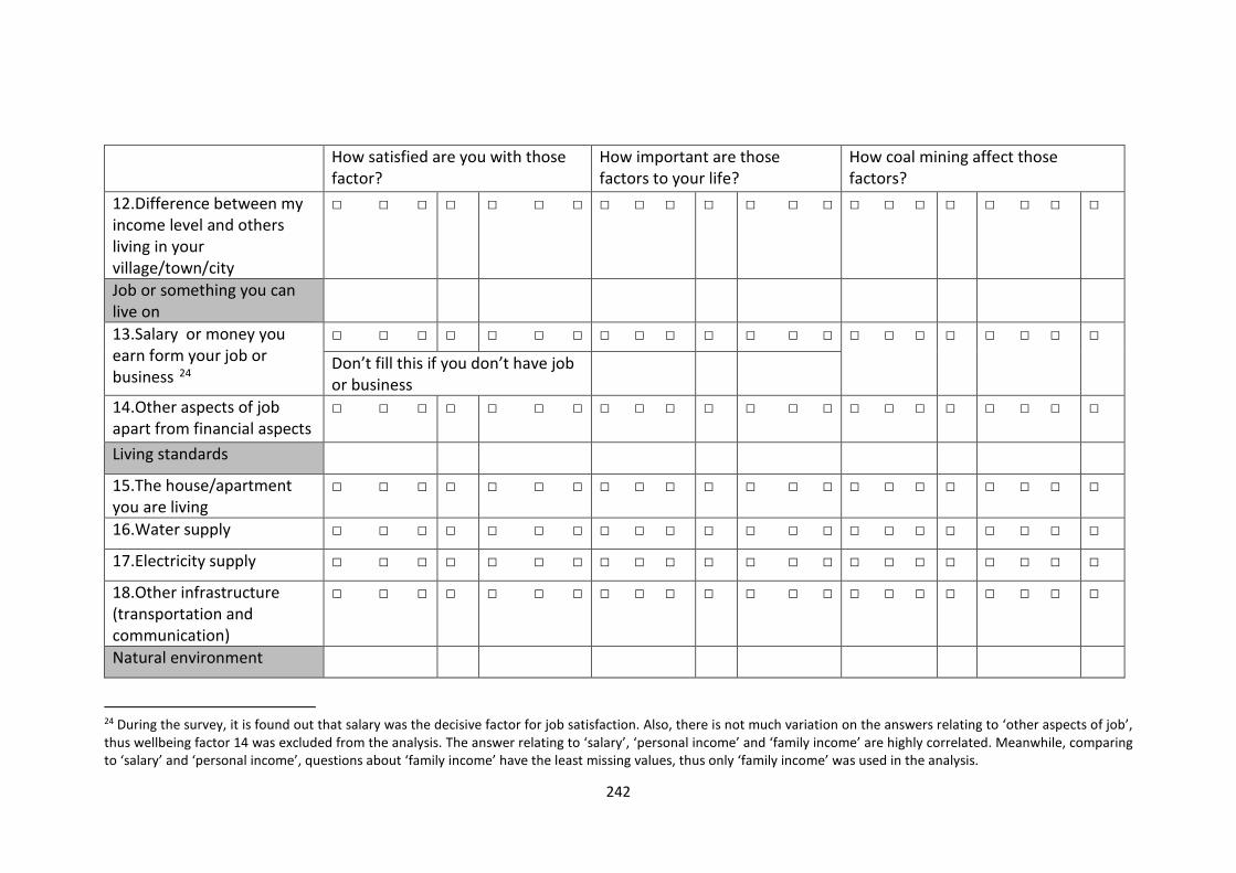
242




12.Difference between my income level and others living in your village/town/city

□ □ □ □ □ □ □ □ □ □ □ □ □ □ □ □ □ □ □ □ □ □

Job or something you can live on

13.Salary or money you earn form your job or business 24

□ □ □ □ □ □ □ □ □ □ □ □ □ □ □ □ □ □ □ □ □ □

Don’t fill this if you don’t have job or business

14.Other aspects of job apart from financial aspects

□ □ □ □ □ □ □ □ □ □ □ □ □ □ □ □ □ □ □ □ □ □

Living standards

15.The house/apartment you are living

□ □ □ □ □ □ □ □ □ □ □ □ □ □ □ □ □ □ □ □ □ □

16.Water supply □ □ □ □ □ □ □ □ □ □ □ □ □ □ □ □ □ □ □ □ □ □

17.Electricity supply □ □ □ □ □ □ □ □ □ □ □ □ □ □ □ □ □ □ □ □ □ □

18.Other infrastructure (transportation and communication)

□ □ □ □ □ □ □ □ □ □ □ □ □ □ □ □ □ □ □ □ □ □

Natural environment

24 During the survey, it is found out that salary was the decisive factor for job satisfaction. Also, there is not much variation on the answers relating to ‘other aspects of job’, thus wellbeing factor 14 was excluded from the analysis. The answer relating to ‘salary’, ‘personal income’ and ‘family income’ are highly correlated. Meanwhile, comparing to ‘salary’ and ‘personal income’, questions about ‘family income’ have the least missing values, thus only ‘family income’ was used in the analysis.

243




19.Total air quality25 □ □ □ □ □ □ □ □ □ □ □ □ □ □ □ □ □ □ □ □ □ □

20.Cleanliness of the air ( whether the air make you sick)

□ □ □ □ □ □ □ □ □ □ □ □ □ □ □ □ □ □ □ □ □ □

21. Dust in the air □ □ □ □ □ □ □ □ □ □ □ □ □ □ □ □ □ □ □ □ □ □

22. Safety of drinking water □ □ □ □ □ □ □ □ □ □ □ □ □ □ □ □ □ □ □ □ □ □

23. Safety of surface water □ □ □ □ □ □ □ □ □ □ □ □ □ □ □ □ □ □ □ □ □ □

Price level

24. House price level □ □ □ □ □ □ □ □ □ □ □ □ □ □ □ □ □ □ □ □ □ □

25.The current price of necessity (food, cloth, transportation)

□ □ □ □ □ □ □ □ □ □ □ □ □ □ □ □ □ □ □ □ □ □

26.Inflation rate □ □ □ □ □ □ □ □ □ □ □ □ □ □ □ □ □ □ □ □ □ □

Education

27.The education opportunity

□ □ □ □ □ □ □ □ □ □ □ □ □ □ □ □ □ □ □ □ □ □

25 Questionnaire for this study, initially, asked about people’s satisfaction dust in the air, air cleanliness, smell of the air, the amount of smoggy days. After the pilot survey, “smell of the air”, and “the amount of smoggy days” were deleted, as rural respondents, generally did not encounter bad smell and smoggy days. Satisfaction with air quality as a whole were also asked after pilot test.

244




28.The quality of education (amount and quality of schools )

□ □ □ □ □ □ □ □ □ □ □ □ □ □ □ □ □ □ □ □ □ □

Personal relationships

29.The relationship status with your family

□ □ □ □ □ □ □ □ □ □ □ □ □ □ □ □ □ □ □ □ □ □

30.Relationship with your close friends, relatives and neighbour

□ □ □ □ □ □ □ □ □ □ □ □ □ □ □ □ □ □ □ □ □ □

31.Social participation (political activity, sports, donation, volunteer, club, religion and so on)

□ □ □ □ □ □ □ □ □ □ □ □ □ □ □ □ □ □ □ □ □ □

Social trust and justice

32.People in the community can trust each other(no cheating and stealing)

□ □ □ □ □ □ □ □ □ □ □ □ □ □ □ □ □ □ □ □ □ □

33.People in the community help each other (carry bag for strange senior people )

□ □ □ □ □ □ □ □ □ □ □ □ □ □ □ □ □ □ □ □ □ □

34.People in the community can be honest to each other

□ □ □ □ □ □ □ □ □ □ □ □ □ □ □ □ □ □ □ □ □ □

245




35.People in the community can count government or police when they need

□ □ □ □ □ □ □ □ □ □ □ □ □ □ □ □ □ □ □ □ □ □

36.Income fairness □ □ □ □ □ □ □ □ □ □ □ □ □ □ □ □ □ □ □ □ □ □

Safety

Physical safety in the place you are living (don’t worry someone harm you)

□ □ □ □ □ □ □ □ □ □ □ □ □ □ □ □ □ □ □ □ □ □

The illegal behaviour your property have encountered (stealing, rob, cheating )

□ □ □ □ □ □ □ □ □ □ □ □ □ □ □ □ □ □ □ □ □ □

39. 40. 41.

Are there other things important to you which we haven’t listed? Please add to the blank and fill the form like other factors.

246

Background information

42. Gender: □Male □female

43. Age: □ 18–25 □ 26–35 □ 36–45 □46–55 □56–65

□above 65

44. How many people, including yourself, normally live in your household?

Adults____ children (16 and younger) ____

45. Marriage status

□Married □ Never Married □ Divorced Widowed □Separated but not divorced

46. The highest level of education of yourself:

□Primary school □ Secondary school □High school □University □Other (please specify)

47. Which of the following categories applies to you?

□Full time paid employment □Part time paid employment □Casual employment

□Unemployment □Full time study □Part time study

48. Please indicate which of the following industries is the main source of your household’s income?

□Agriculture, forestry, animal husbandry or fishing □ Mining □ Manufacturing

□Produce and supply of electricity, gas and water □Construction □Retail

□Transportation, warehousing and postal industry

□Information transferring, IT service and software industry □ Financial industry

□ Accommodation cafes and restaurants □Real estate industry □Leasing and business service

□ Research, technique service and geological exploration □ Education

□Communal facilities management □Culture, sports and entertainment

247

□Public health, social security and social welfare □ Public administration and social organization

49. On average, how much pre–tax income does your household earn each year?

□Below 10,000 □10,000 – 20,000 □20,000 – 30,000 □40,000 – 50,000 □50,000

–60,000 □60,000 – 70,000 □70,000 – 80,000 □ 80,000 – 90,000 □90,000 –

100,000 □100,000 – 110,000 □110,000 – 120,000 □above 120,000 □Prefer not

to say □ I don’t know

50. I spend___hours per week on work, and ___hours per week on leisure, entertainment or sports per week.

51. The number of rooms per person have in average in my dwelling is_

52. I □have / □don’t have flush toilet or bathroom in my dwelling.

53. How far is the following activity related to coal mining from your dwelling? Unit: km

0–10

10–20

20–30

30–40

40–50

50–60

60–70

70–80

80–90

90–100

Coal mining Railway mainly for coal transportation

Coal stockpile Waste from coal

54. Which direction is the following activity related to coal mining from your dwelling?

north northeast northwest South Southeast southwest west east Coal mining Railway mainly for coal transportation

Coal stockpile Coal gangue

55. How are you satisfied with your life as a whole, on a scale from 0 to 100?

248

Appendix A–2: Information sheet

INFORMATION SHEET

PROJECT TITLE: “Coal Mining and Human Wellbeing”

You are invited to take part in a research project about coal Ming and Well–being. The study is being conducted by Qian Li will contribute to the degree in PhD at James Cook University.

If you agree to be involved in the study, you will be invited to complete a questionnaire, which asks you about your assessment of your own life satisfaction. The questionnaire should only take 10 minutes to complete.

Taking part in this study is completely voluntary and you can stop taking part in the study at any time without explanation or prejudice.

Your responses and contact details will be strictly confidential. The data from the study will be used in research publications and reports. You will not be identified in any way in these publications.

If you have any questions about the study, please contact – Qian Li and David King.

Principal Investigator:

Qian Li

School of Education

James Cook University

Phone: 4781 4877

Email: [email protected]

Supervisor: (If applicable) or Co–Investigator Details:

Name: David King

School: School of earth and environment

James Cook University (or other institution)

Phone: (07) 4781 4430

Email: david.king@ jcu.edu.au If you have any concerns regarding the ethical conduct of the study, please contact: Human Ethics, Research Office James Cook University, Townsville, Qld, 4811 Phone: (07) 4781 5011 ([email protected])

249

Appendix B: Comparison of income between the (coal) mining industry and other industries

Table 1 statistical tests between family income of coal mining industry and other industries

Location

Proportion

of family

income

sourced

from coal

mining

Average family income Result from Mann–

whitney Test

Coal mining Non–coal mining P–Value

(2–sided)

P–Value

(1–sided)

Rural With 32.10% 39237 31210 0.0368 0.0184

Rural Close 16.20% 41071 31084 0.0122 0.0061

Urban Close 14.80% 42895 31667 0.6408 0.3204

Urban Far 0.00%

Rural Far 0.00%

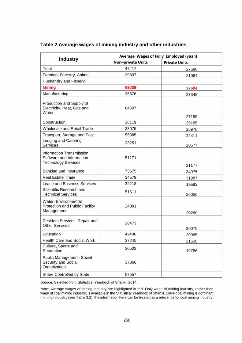
250

Table 2 Average wages of mining industry and other industries

Industry Average Wages of Fully Employed (yuan) Non–private Units Private Units

Total 47417 27580 Farming, Forestry, Animal 29807 21064 Husbandry and Fishery Mining 69039 37694 Manufacturing 36876 27348

Production and Supply of Electricity, Heat, Gas and Water

64507

27199 Construction 38119 29185 Wholesale and Retail Trade 33075 25978 Transport, Storage and Post 55385 22411 Lodging and Catering Services 23251 20577

Information Transmission, Software and Information Technology Services

51171

21177 Banking and Insurance 73675 34975 Real Estate Trade 34579 31987 Lease and Business Services 32218 19582 Scientific Research and Technical Services 51611 26056

Water, Environmental Protection and Public Facility Management

24091 20260

Resident Services, Repair and Other Services 28473

20070 Education 42430 20985 Health Care and Social Work 37245 21526 Culture, Sports and Recreation 36502 19786 Public Management, Social Security and Social Organization

37866

Share Controlled by State 57557

Source: Selected from Statistical Yearbook of Shanxi, 2014

Note: Average wages of mining industry are highlighted in red. Only wage of mining industry, rather than wage of coal mining industry, is available in the Statistical Yearbook of Shanxi. Since coal mining is dominant (mining) industry (see Table 3.2), the information here can be treated as a reference for coal mining industry.

251

Appendix C: The relationship between objective and subjective wellbeing indicators

Appendix C–1: The relationship between actual family income and satisfaction

with income

Table 1 Ordinal regression results (Total sample population)

SatIncome Coef. Std. Err. z P>z [95% Conf. Interval]

income 2.42E–

05 3.10E–

06 7.78 0 1.81E–

05 3.02E–

05 schooling –0.032 0.028 –1.130 0.257 –0.086 0.023 adult –0.052 0.057 –0.920 0.358 –0.163 0.059 children –0.103 0.089 –1.150 0.250 –0.278 0.072 age 0.023 0.008 2.830 0.005 0.007 0.038 female –0.290 0.170 –1.710 0.088 –0.624 0.043 NotPartnered 0.298 0.265 1.120 0.261 –0.221 0.816 emp1 1.442 0.361 4.000 0.000 0.735 2.149 emp2 0.014 0.234 0.060 0.953 –0.444 0.472 emp3 0.383 0.382 1.000 0.316 –0.366 1.132 emp4 0.198 0.202 0.980 0.327 –0.198 0.594

Table 2 Ordinal regression results (Urban Close)

SatIncome Coef. Std. Err. t P>t [95% Conf. Interval]

income 1.73E–

05 6.01E–

06 2.88 0.004 5.50E–

06 2.91E–

05 schooling –0.120 0.081 –1.480 0.139 –0.279 0.039 adult 0.272 0.117 2.320 0.021 0.042 0.502 children 0.380 0.362 1.050 0.294 –0.331 1.092 age 0.044 0.031 1.430 0.154 –0.017 0.104 1.female 0.310 0.431 0.720 0.473 –0.536 1.156 1.NotPartnered 1.338 0.774 1.730 0.084 –0.182 2.858 1.emp1 1.792 1.414 1.270 0.205 –0.985 4.570 1.emp2 1.185 0.866 1.370 0.172 –0.517 2.887 1.emp3 0.371 0.700 0.530 0.596 –1.003 1.745 1.emp4 0.918 0.513 1.790 0.074 –0.091 1.926

252

Table 3 Ordinal regression results (Rural With)


income 2.35E–

05 9.15E–

06 2.57 0.01 5.56E–

06 4.15E–

05 schooling –0.021 0.058 –0.360 0.721 –0.135 0.093 adult –0.212 0.101 –2.100 0.036 –0.411 –0.013 children –0.142 0.167 –0.850 0.397 –0.471 0.187 age 0.005 0.014 0.340 0.732 –0.023 0.033 1.female –0.305 0.307 –0.990 0.321 –0.907 0.298 1.NotPartnered –0.005 0.538 –0.010 0.993 –1.063 1.053 1.emp1 2.262 0.575 3.930 0.000 1.132 3.393 1.emp2 –0.198 0.352 –0.560 0.573 –0.890 0.493 1.emp3 0.730 0.747 0.980 0.329 –0.739 2.198 1.emp4 0.431 0.426 1.010 0.312 –0.405 1.267

Table 4 Ordinal regression results (Rural Close)


income 3.21E–

05 1.06E–

05 3.02 0.003 1.13E–

05 0.000053 schooling –0.037 0.049 –0.750 0.452 –0.132 0.059 adult 0.030 0.096 0.310 0.757 –0.159 0.218 children –0.078 0.151 –0.520 0.605 –0.376 0.219 age 0.012 0.013 0.940 0.346 –0.013 0.037 1.female –0.421 0.324 –1.300 0.194 –1.058 0.215 1.NotPartnered –0.698 0.466 –1.500 0.135 –1.614 0.219 1.emp1 1.453 0.680 2.140 0.033 0.117 2.789 1.emp2 0.558 0.479 1.170 0.244 –0.382 1.498 1.emp3 1.017 0.619 1.640 0.101 –0.198 2.232 1.emp4 0.184 0.367 0.500 0.616 –0.536 0.904

253

Table 5 Ordinal regression results (Urban Far)


income 6.29E–

05 1.72E–

05 3.66 0 2.91E–

05 9.66E–

05 schooling –0.107 0.180 –0.590 0.553 –0.461 0.247 adult –0.441 0.368 –1.200 0.231 –1.163 0.282 children –0.332 0.694 –0.480 0.632 –1.695 1.030 age 0.094 0.047 2.000 0.046 0.002 0.186 1.female –0.753 0.876 –0.860 0.390 –2.474 0.968 1.NotPartnered 5.421 1.617 3.350 0.001 2.245 8.597 1.emp1 –1.954 2.848 –0.690 0.493 –7.548 3.640 1.emp2 –1.894 1.652 –1.150 0.252 –5.139 1.350 1.emp3 –6.011 1.332 –4.510 0.000 –8.628 –3.394 1.emp4 –2.008 1.106 –1.820 0.070 –4.179 0.164

Table 6 Ordinal regression results (Rural Far)


income 0.000033 9.18E–

06 3.59 0 0.000015 0.000051 schooling 0.014 0.121 0.110 0.909 –0.223 0.251 adult –0.272 0.286 –0.950 0.343 –0.834 0.291 children –0.745 0.358 –2.080 0.038 –1.448 –0.042 age 0.080 0.031 2.550 0.011 0.018 0.141 1.female 0.076 0.632 0.120 0.905 –1.165 1.316 1.NotPartnered 1.680 1.290 1.300 0.193 –0.854 4.215 1.emp1 0.699 0.859 0.810 0.416 –0.988 2.386 1.emp2 –1.277 1.096 –1.170 0.244 –3.430 0.875 1.emp3 –0.586 1.131 –0.520 0.605 –2.807 1.636 1.emp4 0.000 0.666 0.000 1.000 –1.307 1.308

254

Appendix C–2: The relationship between PM10 and satisfaction with air

quality


SatAir Coef. Std. Err. z P>z [95% Conf. Interval]

PM10 –0.021 0.002 –9.030 0.000 –0.025 –0.016 schooling –0.073 0.028 –2.590 0.010 –0.129 –0.018 adult 0.139 0.059 2.360 0.018 0.023 0.255 children 0.000 0.088 0.000 0.996 –0.172 0.173 age 0.003 0.008 0.440 0.662 –0.012 0.019 female 0.096 0.173 0.560 0.578 –0.242 0.435 NotPartnered –0.085 0.261 –0.320 0.745 –0.596 0.426 emp1 0.157 0.364 0.430 0.666 –0.556 0.869 emp2 0.182 0.244 0.750 0.455 –0.296 0.660

Table 8 Ordinal regression results (Rural With)

SatAir Coef. Std. Err. t P>t [95% Conf. Interval]

PM10 –0.002 0.004 –0.600 0.551 –0.010 0.005 schooling –0.015 0.054 –0.270 0.785 –0.121 0.091 adult 0.123 0.097 1.270 0.205 –0.067 0.313 children 0.070 0.216 0.320 0.746 –0.354 0.494 age –0.007 0.015 –0.450 0.656 –0.035 0.022 1.female –0.248 0.345 –0.720 0.473 –0.926 0.430 1.NotPartnered 0.620 0.666 0.930 0.352 –0.688 1.928 1.emp1 –1.382 0.892 –1.550 0.122 –3.134 0.369 1.emp2 –0.554 0.463 –1.200 0.232 –1.465 0.356 1.emp3 0.343 0.876 0.390 0.696 –1.377 2.063 1.emp4 0.014 0.389 0.040 0.971 –0.751 0.778

255

Table 9 Ordinal regression results (Rural Close)

SatAir Coef. Std. Err. t P>t [95% Conf. Interval]

PM10 –0.014 0.005 –3.110 0.002 –0.023 –0.005 schooling –0.077 0.063 –1.230 0.221 –0.200 0.046 adult 0.072 0.112 0.640 0.524 –0.149 0.292 children 0.009 0.133 0.070 0.946 –0.252 0.270 age 0.024 0.015 1.520 0.128 –0.007 0.054 1.female –0.322 0.323 –1.000 0.319 –0.958 0.313 1.NotPartnered 0.130 0.452 0.290 0.773 –0.757 1.017 1.emp1 –0.926 0.689 –1.340 0.179 –2.279 0.427 1.emp2 0.324 0.438 0.740 0.460 –0.536 1.183 1.emp3 1.551 0.482 3.220 0.001 0.605 2.497 1.emp4 0.135 0.383 0.350 0.724 –0.617 0.888

256

Appendix C–3: The relationship between objective indicators of housing

and satisfaction with housing


SatHouse Coef. Std. Err. z P>z

[95% Conf. Interval]

1.bathroom 0.921 0.278 3.320 0.001 0.377 1.466 1.flushingToilet 0.141 0.275 0.510 0.609 -0.399 0.680 roomPerPerson 0.265 0.121 2.200 0.028 0.029 0.502 schooling -0.044 0.028 -1.560 0.118 -0.100 0.011 adult 0.048 0.058 0.830 0.405 -0.065 0.162 children 0.068 0.089 0.760 0.450 -0.108 0.243 age 0.019 0.008 2.390 0.017 0.003 0.034 1.female -0.302 0.170 -1.770 0.076 -0.635 0.032 1.NotPartnered -0.192 0.261 -0.740 0.461 -0.703 0.319 1.emp1 0.544 0.362 1.500 0.133 -0.165 1.252 1.emp2 -0.262 0.240 -1.090 0.275 -0.733 0.209 1.emp3 0.662 0.366 1.810 0.070 -0.055 1.380 1.emp4 0.212 0.202 1.050 0.294 -0.184 0.608

Table 11 Ordinal regression results (Urban close)

SatHouse Coef. Std. Err. t P>t [95% Conf. Interval]

1.bathroom 0.384 1.089 0.350 0.725 –1.756 2.524 1.flushingToilet 1.448 0.982 1.470 0.141 –0.482 3.377 roomPerPerson –0.207 0.366 –0.570 0.572 –0.925 0.512 schooling –0.073 0.073 –0.990 0.320 –0.216 0.071 adult –0.022 0.152 –0.140 0.885 –0.320 0.276 children 0.316 0.355 0.890 0.374 –0.382 1.014 age 0.081 0.039 2.070 0.039 0.004 0.157 1.female –0.269 0.521 –0.520 0.606 –1.292 0.755 1.NotPartnered 0.704 0.785 0.900 0.370 –0.837 2.246 1.emp1 0.568 1.575 0.360 0.719 –2.526 3.662 1.emp2 –0.438 1.130 –0.390 0.698 –2.657 1.781 1.emp3 0.907 0.718 1.260 0.207 –0.502 2.317 1.emp4 –0.089 0.622 –0.140 0.887 –1.311 1.134

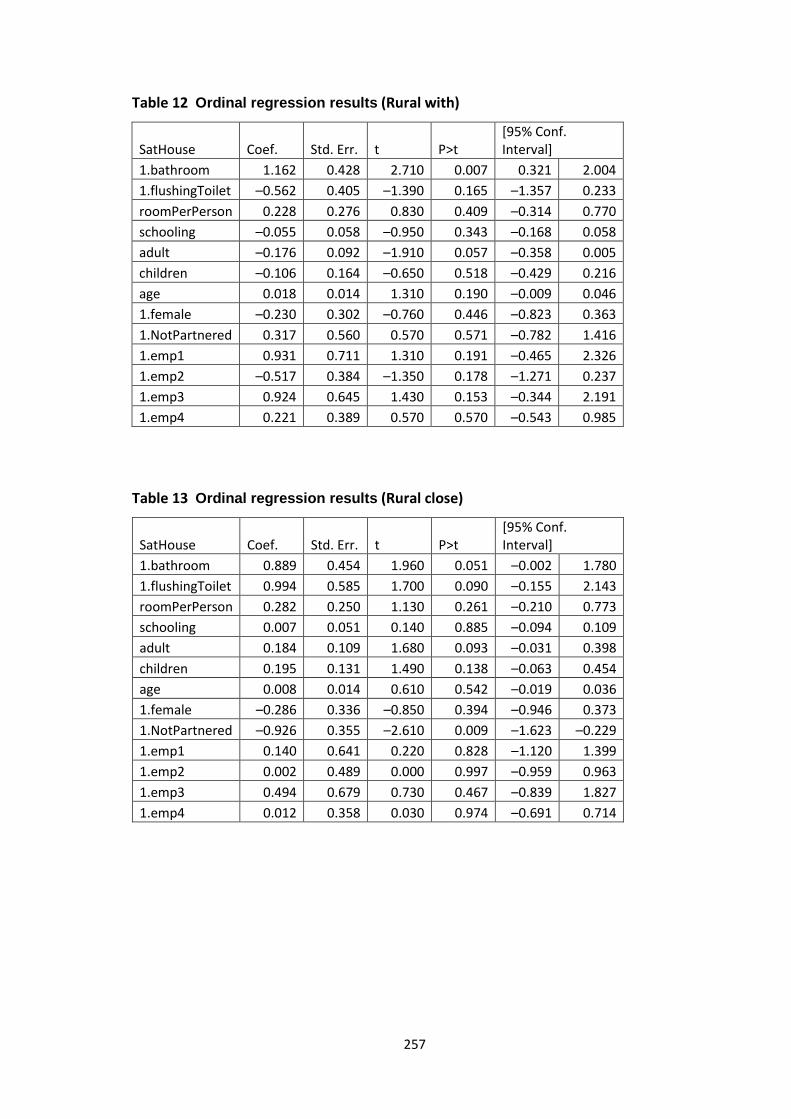
257

Table 12 Ordinal regression results (Rural with)


1.bathroom 1.162 0.428 2.710 0.007 0.321 2.004 1.flushingToilet –0.562 0.405 –1.390 0.165 –1.357 0.233 roomPerPerson 0.228 0.276 0.830 0.409 –0.314 0.770 schooling –0.055 0.058 –0.950 0.343 –0.168 0.058 adult –0.176 0.092 –1.910 0.057 –0.358 0.005 children –0.106 0.164 –0.650 0.518 –0.429 0.216 age 0.018 0.014 1.310 0.190 –0.009 0.046 1.female –0.230 0.302 –0.760 0.446 –0.823 0.363 1.NotPartnered 0.317 0.560 0.570 0.571 –0.782 1.416 1.emp1 0.931 0.711 1.310 0.191 –0.465 2.326 1.emp2 –0.517 0.384 –1.350 0.178 –1.271 0.237 1.emp3 0.924 0.645 1.430 0.153 –0.344 2.191 1.emp4 0.221 0.389 0.570 0.570 –0.543 0.985

Table 13 Ordinal regression results (Rural close)


1.bathroom 0.889 0.454 1.960 0.051 –0.002 1.780 1.flushingToilet 0.994 0.585 1.700 0.090 –0.155 2.143 roomPerPerson 0.282 0.250 1.130 0.261 –0.210 0.773 schooling 0.007 0.051 0.140 0.885 –0.094 0.109 adult 0.184 0.109 1.680 0.093 –0.031 0.398 children 0.195 0.131 1.490 0.138 –0.063 0.454 age 0.008 0.014 0.610 0.542 –0.019 0.036 1.female –0.286 0.336 –0.850 0.394 –0.946 0.373 1.NotPartnered –0.926 0.355 –2.610 0.009 –1.623 –0.229 1.emp1 0.140 0.641 0.220 0.828 –1.120 1.399 1.emp2 0.002 0.489 0.000 0.997 –0.959 0.963 1.emp3 0.494 0.679 0.730 0.467 –0.839 1.827 1.emp4 0.012 0.358 0.030 0.974 –0.691 0.714

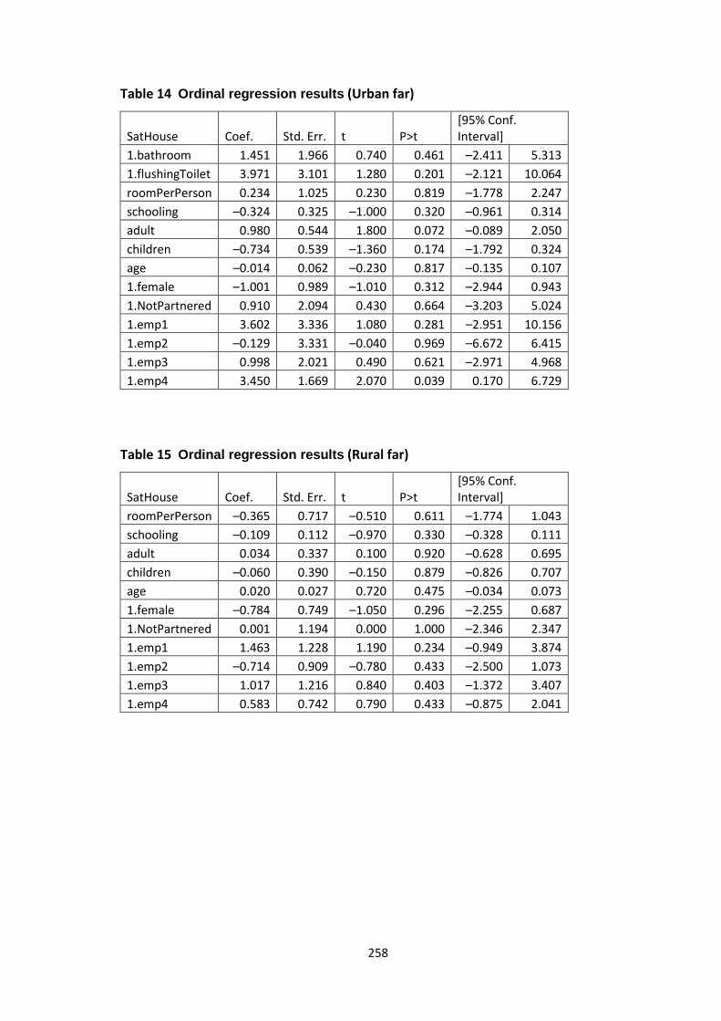
258

Table 14 Ordinal regression results (Urban far)


1.bathroom 1.451 1.966 0.740 0.461 –2.411 5.313 1.flushingToilet 3.971 3.101 1.280 0.201 –2.121 10.064 roomPerPerson 0.234 1.025 0.230 0.819 –1.778 2.247 schooling –0.324 0.325 –1.000 0.320 –0.961 0.314 adult 0.980 0.544 1.800 0.072 –0.089 2.050 children –0.734 0.539 –1.360 0.174 –1.792 0.324 age –0.014 0.062 –0.230 0.817 –0.135 0.107 1.female –1.001 0.989 –1.010 0.312 –2.944 0.943 1.NotPartnered 0.910 2.094 0.430 0.664 –3.203 5.024 1.emp1 3.602 3.336 1.080 0.281 –2.951 10.156 1.emp2 –0.129 3.331 –0.040 0.969 –6.672 6.415 1.emp3 0.998 2.021 0.490 0.621 –2.971 4.968 1.emp4 3.450 1.669 2.070 0.039 0.170 6.729

Table 15 Ordinal regression results (Rural far)


roomPerPerson –0.365 0.717 –0.510 0.611 –1.774 1.043 schooling –0.109 0.112 –0.970 0.330 –0.328 0.111 adult 0.034 0.337 0.100 0.920 –0.628 0.695 children –0.060 0.390 –0.150 0.879 –0.826 0.707 age 0.020 0.027 0.720 0.475 –0.034 0.073 1.female –0.784 0.749 –1.050 0.296 –2.255 0.687 1.NotPartnered 0.001 1.194 0.000 1.000 –2.346 2.347 1.emp1 1.463 1.228 1.190 0.234 –0.949 3.874 1.emp2 –0.714 0.909 –0.780 0.433 –2.500 1.073 1.emp3 1.017 1.216 0.840 0.403 –1.372 3.407 1.emp4 0.583 0.742 0.790 0.433 –0.875 2.041

259

Appendix C– 4: The relationship between objective and subjective

indicators of education

Table 16 OLS regression results – with dependent variable being subjective measures

of respondent satisfaction with education opportunity (Total sample population)

SATeduopp Coef. Std. Err. t P>t [95% Conf. Interval]

schooling -0.011 0.030 -0.380 0.706 -0.069 0.047 children -0.007 0.093 -0.070 0.940 -0.190 0.176 adult 0.019 0.061 0.310 0.755 -0.100 0.138 age -0.015 0.008 -1.850 0.066 -0.031 0.001 female -0.126 0.182 -0.690 0.489 -0.482 0.231 NotPartnered -0.456 0.275 -1.660 0.098 -0.996 0.085 emp1 0.186 0.361 0.510 0.608 -0.524 0.895 emp2 0.071 0.248 0.290 0.774 -0.416 0.558 emp3 -0.251 0.408 -0.620 0.538 -1.053 0.550 emp4 -0.275 0.217 -1.270 0.204 -0.701 0.150 _cons 4.817 0.584 8.250 0.000 3.669 5.964

Table 17 OLS Regression results – with dependent variable being subjective measures

of respondent satisfaction with education quality (Total sample population)

Q281eduqua Coef. Std. Err. t P>t [95% Conf. Interval]

schooling -0.043 0.028 -1.500 0.135 -0.098 0.013 adult 0.021 0.058 0.360 0.716 -0.093 0.136 children -0.154 0.089 -1.730 0.085 -0.330 0.021 age -0.015 0.008 -1.870 0.062 -0.030 0.001 female -0.438 0.174 -2.520 0.012 -0.780 -0.096 NotPartnered -0.264 0.263 -1.000 0.316 -0.782 0.253 emp1 0.234 0.346 0.680 0.500 -0.446 0.914 emp2 -0.085 0.238 -0.360 0.720 -0.552 0.382 emp3 -0.117 0.391 -0.300 0.765 -0.884 0.651 emp4 -0.158 0.208 -0.760 0.447 -0.566 0.250 _cons 5.441 0.560 9.720 0.000 4.342 6.540

260

Appendix D: Ordinal regression – Impacts of coal mining on subjective wellbeing

Appendix D–1: Ordinal regression – Impacts of coal mining on

satisfaction with different life domains

Table 1 Satisfaction with human capital – Urban areas

MFhumcap Coef.

Linearized Std. Err. t P>t


1.FarCoal 0.056 0.373 0.150 0.882 -0.677 0.788 1.miningincome -0.048 0.640 -0.070 0.940 -1.304 1.209 income 0.000 0.000 2.360 0.018 0.000 0.000 children 0.037 0.253 0.150 0.883 -0.460 0.535 adult 0.073 0.126 0.580 0.559 -0.174 0.320 age 0.046 0.024 1.890 0.059 -0.002 0.094 1.female 0.358 0.405 0.880 0.378 -0.438 1.154 1.NotPartnered 1.189 0.578 2.060 0.040 0.053 2.326 schooling -0.019 0.056 -0.330 0.741 -0.129 0.092 1.emp1 0.274 1.018 0.270 0.788 -1.725 2.274 1.emp2 -0.065 0.666 -0.100 0.922 -1.374 1.244 1.emp3 -0.453 0.647 -0.700 0.484 -1.724 0.819 1.emp4 0.447 0.489 0.910 0.361 -0.514 1.408

Table 2 Satisfaction with human capital – Rural areas

SAThumcap Coef. Linearized Std. Err. t P>t


1.WithCoal 0.174 0.226 0.770 0.441 –0.269 0.617 1.FarCoal 0.339 0.271 1.250 0.211 –0.192 0.870 1.miningincome 0.534 0.389 1.370 0.170 –0.230 1.298 1.withminy –0.373 0.472 –0.790 0.430 –1.301 0.554 income 0.000 0.000 3.180 0.002 0.000 0.000 children –0.063 0.102 –0.620 0.534 –0.264 0.137 adult 0.037 0.069 0.540 0.593 –0.098 0.171 age 0.016 0.008 1.890 0.060 –0.001 0.033 1.female –0.200 0.223 –0.900 0.369 –0.639 0.238 1.NotPartnered –0.338 0.327 –1.030 0.301 –0.981 0.304 schooling –0.026 0.033 –0.770 0.439 –0.090 0.039 1.emp1 0.455 0.417 1.090 0.276 –0.364 1.273 1.emp2 –0.527 0.286 –1.840 0.066 –1.088 0.034 1.emp3 0.077 0.476 0.160 0.872 –0.859 1.012 1.emp4 0.149 0.244 0.610 0.542 –0.331 0.629

261

Table 3 Satisfaction with environment – Urban areas

MFenvi Coef.



1.FarCoal 1.264 0.500 2.530 0.012 0.281 2.247 1.miningincome 0.898 0.488 1.840 0.066 -0.060 1.856 income 0.000 0.000 0.610 0.539 0.000 0.000 children -0.315 0.266 -1.180 0.238 -0.838 0.209 adult -0.096 0.188 -0.510 0.611 -0.464 0.273 age 0.011 0.020 0.550 0.585 -0.029 0.051 1.female -0.593 0.465 -1.280 0.202 -1.506 0.320 1.NotPartnered -0.380 0.492 -0.770 0.440 -1.347 0.587 schooling 0.032 0.068 0.470 0.642 -0.102 0.166 1.emp1 1.831 0.747 2.450 0.015 0.364 3.297 1.emp2 0.711 0.709 1.000 0.317 -0.682 2.103 1.emp3 1.133 0.524 2.160 0.031 0.105 2.161 1.emp4 -0.262 0.514 -0.510 0.611 -1.272 0.749

Table 4 Satisfaction with environment – Rural areas

MFenvi Coef.



1.WithCoal -0.796 0.241 -3.300 0.001 -1.270 -0.322 1.FarCoal 2.424 0.324 7.480 0.000 1.787 3.060 1.miningincome -0.204 0.380 -0.540 0.592 -0.950 0.543 1.withminy 0.063 0.453 0.140 0.889 -0.827 0.953 income 0.000 0.000 -0.240 0.809 0.000 0.000 children -0.027 0.091 -0.300 0.767 -0.205 0.152 adult 0.051 0.065 0.790 0.431 -0.076 0.178 age 0.013 0.008 1.540 0.125 -0.004 0.029 1.female 0.072 0.191 0.380 0.707 -0.304 0.448 1.NotPartnered 0.400 0.298 1.340 0.180 -0.185 0.984 schooling -0.106 0.034 -3.160 0.002 -0.173 -0.040 1.emp1 -0.382 0.363 -1.050 0.293 -1.096 0.332 1.emp2 0.034 0.244 0.140 0.889 -0.446 0.514 1.emp3 1.169 0.454 2.570 0.010 0.276 2.062 1.emp4 0.160 0.244 0.650 0.513 -0.320 0.640

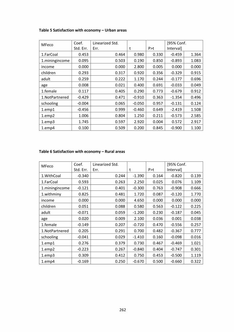
262

Table 5 Satisfaction with economy – Urban areas

MFeco Coef. Std. Err.



1.FarCoal 0.453 0.464 0.980 0.330 -0.459 1.364 1.miningincome 0.095 0.503 0.190 0.850 -0.893 1.083 income 0.000 0.000 2.800 0.005 0.000 0.000 children 0.293 0.317 0.920 0.356 -0.329 0.915 adult 0.259 0.222 1.170 0.244 -0.177 0.696 age 0.008 0.021 0.400 0.691 -0.033 0.049 1.female 0.117 0.405 0.290 0.773 -0.679 0.912 1.NotPartnered -0.429 0.471 -0.910 0.363 -1.354 0.496 schooling -0.004 0.065 -0.050 0.957 -0.131 0.124 1.emp1 -0.456 0.999 -0.460 0.649 -2.419 1.508 1.emp2 1.006 0.804 1.250 0.211 -0.573 2.585 1.emp3 1.745 0.597 2.920 0.004 0.572 2.917 1.emp4 0.100 0.509 0.200 0.845 -0.900 1.100

Table 6 Satisfaction with economy – Rural areas

MFeco Coef. Std. Err.



1.WithCoal -0.340 0.244 -1.390 0.164 -0.820 0.139 1.FarCoal 0.593 0.263 2.250 0.025 0.076 1.109 1.miningincome -0.121 0.401 -0.300 0.763 -0.908 0.666 1.withminy 0.825 0.481 1.720 0.087 -0.120 1.770 income 0.000 0.000 4.650 0.000 0.000 0.000 children 0.051 0.088 0.580 0.563 -0.122 0.225 adult -0.071 0.059 -1.200 0.230 -0.187 0.045 age 0.020 0.009 2.100 0.036 0.001 0.038 1.female -0.149 0.207 -0.720 0.470 -0.556 0.257 1.NotPartnered 0.205 0.291 0.700 0.482 -0.367 0.777 schooling -0.041 0.029 -1.410 0.160 -0.098 0.016 1.emp1 0.276 0.379 0.730 0.467 -0.469 1.021 1.emp2 -0.223 0.267 -0.840 0.404 -0.747 0.301 1.emp3 0.309 0.412 0.750 0.453 -0.500 1.119 1.emp4 -0.169 0.250 -0.670 0.500 -0.660 0.322

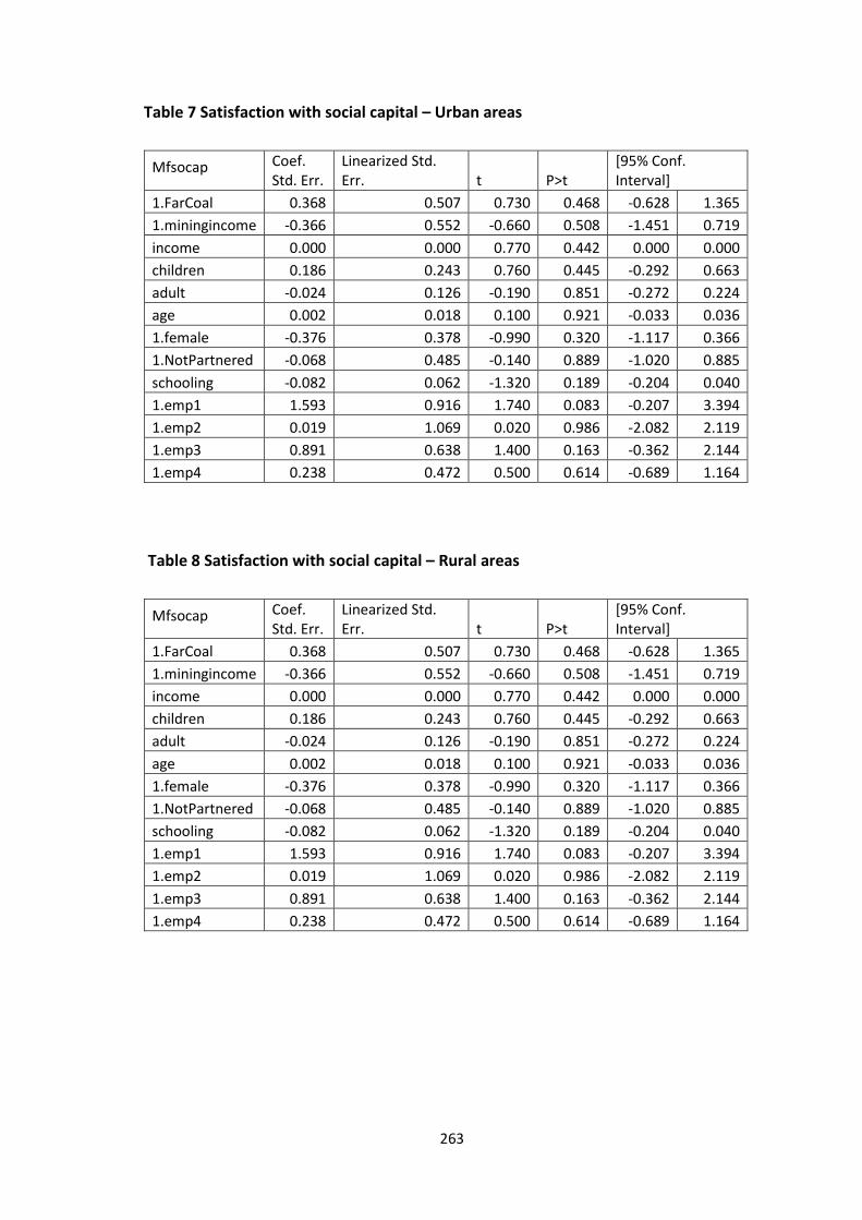
263

Table 7 Satisfaction with social capital – Urban areas

Mfsocap Coef. Std. Err.



1.FarCoal 0.368 0.507 0.730 0.468 -0.628 1.365 1.miningincome -0.366 0.552 -0.660 0.508 -1.451 0.719 income 0.000 0.000 0.770 0.442 0.000 0.000 children 0.186 0.243 0.760 0.445 -0.292 0.663 adult -0.024 0.126 -0.190 0.851 -0.272 0.224 age 0.002 0.018 0.100 0.921 -0.033 0.036 1.female -0.376 0.378 -0.990 0.320 -1.117 0.366 1.NotPartnered -0.068 0.485 -0.140 0.889 -1.020 0.885 schooling -0.082 0.062 -1.320 0.189 -0.204 0.040 1.emp1 1.593 0.916 1.740 0.083 -0.207 3.394 1.emp2 0.019 1.069 0.020 0.986 -2.082 2.119 1.emp3 0.891 0.638 1.400 0.163 -0.362 2.144 1.emp4 0.238 0.472 0.500 0.614 -0.689 1.164

Table 8 Satisfaction with social capital – Rural areas

Mfsocap Coef. Std. Err.



1.FarCoal 0.368 0.507 0.730 0.468 -0.628 1.365 1.miningincome -0.366 0.552 -0.660 0.508 -1.451 0.719 income 0.000 0.000 0.770 0.442 0.000 0.000 children 0.186 0.243 0.760 0.445 -0.292 0.663 adult -0.024 0.126 -0.190 0.851 -0.272 0.224 age 0.002 0.018 0.100 0.921 -0.033 0.036 1.female -0.376 0.378 -0.990 0.320 -1.117 0.366 1.NotPartnered -0.068 0.485 -0.140 0.889 -1.020 0.885 schooling -0.082 0.062 -1.320 0.189 -0.204 0.040 1.emp1 1.593 0.916 1.740 0.083 -0.207 3.394 1.emp2 0.019 1.069 0.020 0.986 -2.082 2.119 1.emp3 0.891 0.638 1.400 0.163 -0.362 2.144 1.emp4 0.238 0.472 0.500 0.614 -0.689 1.164

264

Table 9 Satisfaction with institutional capital – Urban areas

SATinscap Coef. Linearized Std. Err. t P>t


1.FarCoal 0.474 0.422 1.120 0.262 –0.355 1.303 1.miningincome 0.099 0.488 0.200 0.840 –0.860 1.058 income 0.000 0.000 1.020 0.307 0.000 0.000 children –0.350 0.349 –1.000 0.316 –1.034 0.335 adult 0.161 0.130 1.240 0.216 –0.094 0.415 age 0.028 0.024 1.190 0.234 –0.018 0.074 1.female –0.246 0.423 –0.580 0.561 –1.077 0.584 1.NotPartnered –0.443 0.651 –0.680 0.497 –1.723 0.837 schooling –0.063 0.063 –0.990 0.324 –0.187 0.062 1.emp1 0.517 1.035 0.500 0.618 –1.516 2.550 1.emp2 –0.456 1.086 –0.420 0.675 –2.590 1.678 1.emp3 2.279 0.681 3.350 0.001 0.942 3.616 1.emp4 0.622 0.518 1.200 0.230 –0.395 1.640

Table 10 Satisfaction with institutional capital – Rural areas

MFinscap Coef. Linearized Std. Err. t P>t


1.WithCoal -0.367 0.240 -1.530 0.126 -0.838 0.103 1.FarCoal -0.983 0.290 -3.380 0.001 -1.553 -0.412 1.miningincome 0.037 0.359 0.100 0.918 -0.668 0.742 1.withminy 0.335 0.437 0.770 0.444 -0.524 1.194 income 0.000 0.000 2.290 0.023 0.000 0.000 children -0.120 0.090 -1.330 0.185 -0.298 0.058 adult -0.014 0.065 -0.220 0.830 -0.142 0.114 age 0.007 0.009 0.740 0.463 -0.011 0.025 1.female -0.242 0.190 -1.270 0.203 -0.616 0.131 1.NotPartnered -0.263 0.296 -0.890 0.376 -0.845 0.320 schooling -0.079 0.031 -2.590 0.010 -0.139 -0.019 1.emp1 0.110 0.378 0.290 0.771 -0.632 0.852 1.emp2 -0.109 0.279 -0.390 0.695 -0.657 0.439 1.emp3 0.830 0.401 2.070 0.039 0.042 1.619 1.emp4 0.115 0.230 0.500 0.619 -0.338 0.568

265

Table 11 Satisfaction with living conditions – Urban areas

MFlivcon Coef.



1.FarCoal 0.474 0.422 1.120 0.262 -0.355 1.303 1.miningincome 0.099 0.488 0.200 0.840 -0.860 1.058 income 0.000 0.000 1.020 0.307 0.000 0.000 children -0.350 0.349 -1.000 0.316 -1.034 0.335 adult 0.161 0.130 1.240 0.216 -0.094 0.415 age 0.028 0.024 1.190 0.234 -0.018 0.074 1.female -0.246 0.423 -0.580 0.561 -1.077 0.584 1.NotPartnered -0.443 0.651 -0.680 0.497 -1.723 0.837 schooling -0.063 0.063 -0.990 0.324 -0.187 0.062 1.emp1 0.517 1.035 0.500 0.618 -1.516 2.550 1.emp2 -0.456 1.086 -0.420 0.675 -2.590 1.678 1.emp3 2.279 0.681 3.350 0.001 0.942 3.616 1.emp4 0.622 0.518 1.200 0.230 -0.395 1.640

Table 12 Satisfaction with living conditions – Rural areas

MFlivcon Coef.



1.WithCoal -0.367 0.240 -1.530 0.126 -0.838 0.103 1.FarCoal -0.983 0.290 -3.380 0.001 -1.553 -0.412 1.miningincome 0.037 0.359 0.100 0.918 -0.668 0.742 1.withminy 0.335 0.437 0.770 0.444 -0.524 1.194 income 0.000 0.000 2.290 0.023 0.000 0.000 children -0.120 0.090 -1.330 0.185 -0.298 0.058 adult -0.014 0.065 -0.220 0.830 -0.142 0.114 age 0.007 0.009 0.740 0.463 -0.011 0.025 1.female -0.242 0.190 -1.270 0.203 -0.616 0.131 1.NotPartnered -0.263 0.296 -0.890 0.376 -0.845 0.320 schooling -0.079 0.031 -2.590 0.010 -0.139 -0.019 1.emp1 0.110 0.378 0.290 0.771 -0.632 0.852 1.emp2 -0.109 0.279 -0.390 0.695 -0.657 0.439 1.emp3 0.830 0.401 2.070 0.039 0.042 1.619 1.emp4 0.115 0.230 0.500 0.619 -0.338 0.568

266

Appendix D–2: Ordinal regression – Impacts of coal mining on global life

satisfaction

Table 13 Global life satisfaction – Urban areas

LS Coef.



1.FarCoal -0.462 0.428 -1.080 0.280 -1.302 0.378 1.miningincome -0.698 0.576 -1.210 0.226 -1.829 0.433 income 0.000 0.000 2.880 0.004 0.000 0.000 children 0.370 0.230 1.610 0.108 -0.082 0.823 adult 0.016 0.135 0.120 0.904 -0.248 0.281 age 0.024 0.018 1.330 0.184 -0.011 0.059 1.female -0.657 0.457 -1.440 0.152 -1.555 0.242 1.NotPartnered -0.259 0.675 -0.380 0.702 -1.584 1.067 schooling 0.080 0.062 1.300 0.194 -0.041 0.201 1.emp1 1.305 0.732 1.780 0.075 -0.133 2.743 1.emp2 0.240 0.847 0.280 0.777 -1.424 1.905 1.emp3 0.204 0.871 0.230 0.815 -1.508 1.915 1.emp4 0.244 0.626 0.390 0.697 -0.986 1.475

Table 14 Global life satisfaction – Rural areas

LS Coef.



1.WithCoal -0.339 0.235 -1.450 0.149 -0.800 0.122 1.FarCoal 0.186 0.305 0.610 0.542 -0.414 0.786 1.miningincome -0.079 0.354 -0.220 0.824 -0.774 0.616 1.withminy 1.020 0.459 2.220 0.027 0.119 1.922 income 0.000 0.000 4.070 0.000 0.000 0.000 children -0.012 0.101 -0.110 0.909 -0.209 0.186 adult -0.056 0.066 -0.850 0.397 -0.186 0.074 age 0.010 0.010 1.010 0.311 -0.009 0.029 1.female -0.521 0.213 -2.450 0.015 -0.939 -0.103 1.NotPartnered 0.196 0.358 0.550 0.584 -0.507 0.899 schooling -0.009 0.034 -0.270 0.789 -0.077 0.059 1.emp1 0.839 0.373 2.250 0.025 0.106 1.571 1.emp2 -0.154 0.290 -0.530 0.596 -0.724 0.416 1.emp3 0.330 0.615 0.540 0.592 -0.878 1.538 1.emp4 0.087 0.235 0.370 0.712 -0.376 0.549

coal mining and human wellbeing: a case-study in …...coal mining and human wellbeing: a case-study...

Documents