University of California,Santa Barbara

Senior Thesis

Closed Geodesics onSurfaces of Revolution

Author:Jordan Rainone

Supervisor:Dr. Lee Kennard

May 30, 2014

2

Abstract

In this paper we consider the existence of closed geodesics on closed surfaces, and strengthentheir results in a special case. Bangert and Franks proved that on any closed surface thereare infinitely many geometrically distinct, closed geodesics. Hingston proved a refinement thatcounts the number of such geodesic up to a fixed length. In particular, for surfaces of revolution,the result is trivial. Indeed, there is a circle’s worth of geometrically distinct closed geodesicswhich connect the poles.

This motivated a new notion of distinct geodesics. We say that two geodesics are stronglygeometrically distinct if there is no rotation taking the image of one to the image of the other.Notice that the rotation by zero degrees is admitted, so strongly geometrically distinct geodesicsare also geometrically distinct.

We can now formulate a question that is analogous to the one that Bangert and Franksanswered: On a closed surface of revolution, are there infinitely many strongly geometricallydistinct closed geodesics? Petrics, Borzellino, Jordan-Squire, and Sullivan recently proves this.We provide a self contained proof which somewhat parallels theirs. In addition, we prove ananalogue of Hingston’s refinement that counts the number of strongly geometrically distinctclosed geodesics up to a fixed length.

3

Contents

1 Introduction 4

2 Background 52.1 Riemannian geometry . . . . . . . . . . . . . . . . . . . . . . . . . . . . . . . . . . . 52.2 Surfaces of revolution . . . . . . . . . . . . . . . . . . . . . . . . . . . . . . . . . . . 92.3 Angular momentum and Claurait’s relation . . . . . . . . . . . . . . . . . . . . . . . 12

3 Geodesic behavior 133.1 Meridians and equators . . . . . . . . . . . . . . . . . . . . . . . . . . . . . . . . . . 133.2 Asymptotic geodesics . . . . . . . . . . . . . . . . . . . . . . . . . . . . . . . . . . . . 153.3 Oscillating geodesics . . . . . . . . . . . . . . . . . . . . . . . . . . . . . . . . . . . . 18

4 Length and rotation of a full trip 224.1 Definition . . . . . . . . . . . . . . . . . . . . . . . . . . . . . . . . . . . . . . . . . . 224.2 Integrability . . . . . . . . . . . . . . . . . . . . . . . . . . . . . . . . . . . . . . . . . 294.3 Continuity . . . . . . . . . . . . . . . . . . . . . . . . . . . . . . . . . . . . . . . . . . 324.4 Differentiability . . . . . . . . . . . . . . . . . . . . . . . . . . . . . . . . . . . . . . . 34

5 Results 395.1 Rational points . . . . . . . . . . . . . . . . . . . . . . . . . . . . . . . . . . . . . . . 395.2 Infinitude of closed geodesics . . . . . . . . . . . . . . . . . . . . . . . . . . . . . . . 395.3 Counting . . . . . . . . . . . . . . . . . . . . . . . . . . . . . . . . . . . . . . . . . . 41

6 References 44

4

1 Introduction

A long standing problem in Riemannian geometry is determining the existence of closed geodesics.For some background on this problem, see Berger [2] and the introduction in Hingston [6].

If a closed geodesic does exist, it is natural to wonder whether others, or even infinitely many,exist. Note that two geodesics which have the same image should not be double counted. For thisreason, we are restricted to geometrically distinct geodesics and ask:

Given a complete Riemannian manifold M , are there infinitely many geometrically dis-tinct closed geodesics on M?

This is a broad question. In particular, the answer is yes whenever the manifold has infinitefundamental group. Restricting to the compact, simply connected case, the simplest question is thefollowing:

Given any metric on S2, are there infinitely many geometrically distinct closed geodesics?

The answer is yes, but this was only proven recently by Bangert and Franks (see [1, 5]). As arefinement, Hingston [6] proved that the number of geometrically distinct closed geodesics of lengthless than ` grows at least as fast as the primes (i.e., at least as fast as `/ log `). The proofs requireMorse theory and other advanced techniques.

Our original goal of this paper was to prove the same result using only elementary techniquesin the special case of surfaces of revolution. However, it turns out that the result is trivial in thiscase. Indeed, there is a circle’s worth of geometrically distinct closed geodesics which connect thepoles. This motivated a new notion of ‘distinct’ geodesics. In the background section we definetwo geodesics on a surface of revolution to be strongly geometrically distinct if there is no rotationtaking the image of one to the image of the other. The ultimate goal of this paper is to answer thefollowing question:

On a closed surface of revolution, are there infinitely many strongly geometrically dis-tinct closed geodesics?

We believe that the answer is yes and we suggest the following proof strategy:

1. Define Γ to represent a large class of strongly geometric distinct geodesics. Show that Γ islocally diffeomorphic to R.

2. Define the function R : Γ→ R to be the ‘rotation’ of geodesics represented in Γ.

3. Show that R is a continuous function

4. Show that if R(γ) ∈ 2πQ, then γ is closed.

5. Prove that if R is a constant function then, in fact, R ≡ 2π.

6. Show, using the intermediate value theorem, that if R is not constant then R achieves infinitelymany points in 2πQ. We can use the intermediate value theorem because R is continuous andΓ is locally diffeomorphic to R.

7. Conclude that all closed, simply connected, surfaces of revolution have infinitely many stronglygeometrically distinct closed geodesics.

5

The background section will provide the unfamiliar reader with alll the necessary informationabout Riemannian geometry in general, and surfaces of revolution in specific. Those who are famil-iar with this topic may skip to Section 3.

Section 3 will be devoted to completing Step 1 and laying the ground work needed to completethe rest of the proof. In Section 4 we carry out Steps 2 and 3. The last section will complete theSteps 4 through 7, and thus prove our main result in Theorem 5.2.1.

Once we prove our main result, there are a number of reasonable follow-up questions. To discussthem, let N(`) denote the number of strongly geometrically distinct closed geodesics of length lessthan `.

1. Can we find a lower bound on N(`), thereby proving an analogue of Hingston’s theorem?

2. Can we find an upper bound on N(`), at least for a large collection of surfaces of revolution(e.g., not including the constant curvature metric on S2)?

3. In Hingston’s results, N(`) actually grows quadratically for generic metrics. Is there a similarimprovement in the context of surfaces of revolution?

In this paper we have answered the first question (see Theorem 5.3.1).

2 Background

2.1 Riemannian geometry

A topological manifold M of dimension n, or topological n-manifold, is a topological space whichsatisfies the following properties:

1. M is Hausdorff

2. M is second-countable

3. M is locally Euclidean of dimension n

The third criterion means that for each p ∈M there exists: an open neighborhood U⊆M , an openset V⊆Rn and a homeomorphism φ : V → U . We call the pair (U, φ) a coordinate chart, or some-times just a chart. The short hand p ∈ (U, φ) is often used to denote that (U, φ) is a coordinatechart and that p is in U .

A collection of charts {(Uα, φα)} is called an atlas if it covers the manifold; meaning that forall p ∈M there exists a chart (U, φ) in the atlas such that p ∈ (U, φ).

Given two coordinate charts (U, φ) and (V, ψ) we call the functions ψ−1 ◦ φ : φ−1(U ∩ V ) →ψ−1(U ∩ V ) and φ−1 ◦ ψ : ψ−1(U ∩ V )→ φ−1(U ∩ V ) transition maps.

A smooth manifold is a topological manifold equipped with an atlas where all transition mapsare smooth. Here the word smooth means infinitely times differentiable and is synonymous withC∞. Examples of smooth manifolds include: Rn, Sn (the n-sphere), Tn (the n-dimensional Torus),

6

RPn (n-dimensional Real Projective Space), etc...

Smooth manifolds are very useful because we are able to preform calculus on them. This meansthat we can extend the notion of differentiability to functions defined on smooth manifolds.. In-deed, if M and N are smooth manifolds then a function F : M → N is said to be smooth ifψ−1 ◦ F ◦ φ : φ−1(U)→ ψ−1(F (U)) is smooth for every pair of charts (U, φ) for M and (F (U), ψ)for N . Notice that this definition coincides with vector calculus definition of smoothness whenM = Rm and N = Rn. A map F : M → N is said to be a diffeomorphism if it is a smooth bijectionwith a smooth inverse. The existence of such a map is an equivalence relation between M and N .Notice that if (U, φ) is a coordinate chart then φ : φ−1(U)→ U is a diffeomorphism.

When studying a smooth n-manifold M we come across its tangent bundle, which we denoteby TM . This space is constructed by taking the disjoint union of one copy of Rn for every p ∈M .We arrange these copies of Rn by making each one the tangent plane to M at some point p ∈ M ,which we denote by TpM . Intuitively this is a collection of linear approximation of M . Vectors inTpM correspond loosely to directional derivatives of smooth real valued functions on M .

If (U, φ) is a chart for M then φ sends points in some open subset V⊆Rn to U⊆M . Similarly,if we let p ∈ (U, φ) and q = φ−1(p), then the differential of φ at q, dφ|q : TqRn → TpM , sendsthe tangent vectors at q to the the tangent vectors at p. The vectors in TqRn are just the partial

derivatives operators at q, forming an n dimensional vector space with basis{

∂∂xj

∣∣q

}nj=1

where

x1, . . . , xn are the canonical coordinated on Rn. Using dφ|q we identify the vector ∂∂xj

∣∣q

with its

image dφ|q(

∂∂xj

∣∣q

)and usually denote it by ∂

∂xj

∣∣p. The set

{∂∂xi

∣∣p

}is called the coordinate basis

of TpM corresponding to φ.

Let us make this relation between tangent vectors and directional derivatives more clear. Ifp ∈ (U, φ) with φ(q) = p and f : U → R is a smooth function, then we can apply ∂

∂xi

∣∣p

to f

by defining ∂∂xi

∣∣p

(f) := ∂

∂xi(f ◦ φ)(q). We can extend this definition to any v ∈ TpM using lin-

earity. Suppose writing v as a linear combination of ∂∂xi

∣∣p

gives us v = ai ∂∂xi

∣∣p

where ai ∈ R,

then v(f) := ai ∂∂xi

(f ◦ φ)(q)(

note that we are using the Einstein Summation Notation where

ai ∂∂xi

∣∣p

denotes∑n

i=1 ai ∂∂xi

∣∣p

). However this definition depends on our choice of chart, so we must

make sure that when we express v in different bases we get the same value of v(f).

Let (V, ψ) be another chart containing p and let{

∂∂yi

∣∣p

}be its corresponding coordinate basis

for TpM . Let φ(x1, . . . xn) = p, ψ(y1, . . . yn) = p and define yj : M → R to be the componentfunctions of ψ so that yj(p) = yj . If v ∈ TpM and v = ai ∂

∂xi

∣∣p

then we can transition to the other

7

basis using the chain rule from multivariable calculus:

ai∂

∂xi

∣∣∣p(f) = ai

∂

∂xi(f ◦ φ)(x1, . . . xn)

= ai∂yj

∂xi∂

∂yj(f ◦ φ ◦ (φ−1 ◦ ψ))(y1, . . . yn)

= ai∂yj

∂xi∂

∂yj(f ◦ ψ)(y1, . . . yn)

= ai∂yj

∂xi∂

∂yj

∣∣∣p(f) .

Calculating v(f) using the two different charts yields the same result and thus v(f) is well defined.

As one might have guessed the coordinate basis{

∂∂xi

}for φ is defined on all of U . Using this we

can extend the notion of tangent vector to a vector field. A vector field on U is a smooth functionX : U → TU where X(p) ∈ TpU . By smoothness we mean that if X(p) = ai(p) ∂

∂xi

∣∣p

for all p ∈ Uthen ai : U → R is smooth. X is a vector field on M if it is a vector field on each coordinate chart(U, φ) of M .

Vector fields can also be defined along smooth curves γ : R→M . Let γ((−ε, ε))⊂U and (U, φ)be a chart where γ(t) = φ(x1(t), . . . xn(t)) for t ∈ (−ε, ε). Using the chain rule we can calculate the

derivative of γ to be γ′(t) = dxi

dt (t) ∂∂xj|γ(t) for any t ∈ (−ε, ε). Note that γ′ is a vector field along γ.

We can apply a vector field X : M → TM to a scalar field f : M → R to get a scalar fieldXf : M → R defined by Xf(p) := X|p(f). We can also apply a vector field to another vectorfield but first we need to define a Lie bracket. If X and Y are vector fields, then the Lie bracket[X,Y ] is a vector field defined by [X,Y ](f) := X(Y f) − Y (Xf) where f is a scalar field. Writingthis expression in local coordinates with X = ai ∂

∂xiand Y = bj ∂

∂yjgives us X(Y f) − Y (Xf) =

ai ∂∂xi

(bj ∂f∂xj

) − bj ∂∂xj

(ai ∂f∂xi

). After simplifying we get the vector field [X,Y ] = (ai ∂bj

∂xi− bi ∂aj

∂xi) ∂∂xj

.

Notice that [ ∂∂xi, ∂∂xj

] ≡ 0 for all i and j.

There is another way in which we can apply one vector field to another. This is a generalizationof directional derivatives called a covariant derivative. Let v ∈ TpM , f be a scalar field, α be ascalar and X,Y and Z be vector fields. A covariant derivative, if it exists, is an object D thatsatisfies the following properties:

1) Dvf is a real number and coincides with v(f)2) DvX obeys the product rule (Dv(fX))(p) = f(p)DvX +X(p)Dvf3) DYX is a vector field where (DYX)(p) = DY (p)X4) DYX is function linear in Y so DfY+ZX = fDYX +DZX5) DvX is linear in X so Dv(αX + Y ) = αDvX +DV Y

If M is a smooth manifold then we can endow it with an inner product gp on TpM for eachpoint p ∈M . If g varies in a smooth way then we say (M, g), or sometimes just M , is a Riemannianmanifold. These manifolds have more structure and allow us to define the objects that are going tobe at the center of this paper: geodesics.

A Levi-Civita connection ∇ (pronounced “del” or “nabla”) is defined as a covariant deriva-tive which is both symmetric and compatible with the metric. Symmetry simply means that

8

∇XY −∇YX = [X,Y ]. Compatability with the metric gives us the Leibniz formulaZ (〈X,Y 〉) = 〈∇ZX,Y 〉+ 〈X,∇ZY 〉 where 〈X,Y 〉 |p is the inner product of X|p and Y |p, oftenwritten as gp(X|p, Y |p). Not only does such an object exist for all Reimannian manifolds M , but itis also unique. A proof of the following proposition can be found on page 55 of Do Carmo [4].

Proposition 2.1.1 (The Levi-Civita Connection). Given a Riemannian manifold M and metricg there exists a unique covariant derivative ∇ which satisfies the following properties for all vectorfield X,Y and Z:1) ∇XY −∇YX = [X,Y ] , and2) Z (〈X,Y 〉) = 〈∇ZX,Y 〉+ 〈X,∇ZY 〉.Such a covariant derivative is called the Levi-Civita connection for M , and it can be explicitlycalculated by the following formula:

〈Z,∇YX〉 =1

2[X 〈Y, Z〉+ Y 〈Z,X〉 − Z 〈X,Y 〉 − 〈[X,Z], Y 〉 − 〈[Y,Z], X〉 − 〈[X,Y ], Z〉] .

To avoid having to write down this expression every time we try to compute ∇XY , we define theChristoffel symbols Γkij . The Christoffel symbols are a set functions defined on a coordinate neigh-

borhood (U, φ) that satisfy ∇ ∂

∂xi

∂∂xj

= Γkij∂∂xk

. If X = ai ∂∂xi

and Y = bj ∂∂xj

, then the Christoffel

symbols can be used to calculate

∇XY = ai∂bj

∂xi∂

∂xj+ aibjΓkij

∂

∂xk.

If M is a Riemannian manifold then a geodesic is a smooth curve γ : (a, b)⊆R → M whichsatisfies the following property:

∇γ′γ′ = 0 (2.1)

We can extract more information about this equation by writing it in local coordinates. Letγ(t) = φ(x1(t), . . . xn(t)) and γ′(t) = dxi

dt (t) ∂∂xi

∣∣γ(t)

. Using the product rule we get

∇γ′γ′ =(∇γ′

dxj

dt

)∂

∂xj+dxj

dt

(∇γ′

∂

∂xj

).

Applying γ′ to dxj

dt gives us d2xj

dt2and ∇ ∂

∂xi

∂∂xj

= Γkij∂∂xk

. Hence γ(t) = φ(x1(t), . . . xn(t)) satisfies

(2.1) if and only if

d2xk

dt2= −dx

i

dt

dxj

dtΓkij . (2.2)

This is call the Geodesic Equations. From these, we can get three useful properties. The proofof the first two can be found in Do Carmo pages 60-64 [4].

Proposition 2.1.2 (Constant Speed). All geodesics γ on a Riemannian manifold M have constantspeed. That is, for all geodesics γ : (a, b)→M , there exists a C ≥ 0 such that |γ′(t)| = C.

Proposition 2.1.3 (Existence and Uniqueness). Let M be a Riemannian manifold. Given p ∈Mand a tangent vector v ∈ TpM there exists a unique geodesic γ : (−ε, ε) → M such that γ(0) = pand γ′(0) = v, for some ε > 0.

9

For the next proposition we need to know that an isometry F : M → N is a diffeomorphismbetween Riemannian manifolds where the linear map dF |p : TpM → TF (p)N is an inner productspace isometry.

Proposition 2.1.4 (Isometries). Let M be a Riemannian manifold and F : M → N be an isometry.If γ is a geodesic on M then T ◦ γ is also a geodesic on N .

Proof. For any vector fields X and Y , ∇XY∣∣p

is uniquely determined by the metric gp, as givenby the formula in Proposition 2.1.1. The defining property of an isometry F is that it preservesthe metric; gp(X|p, Y |p) = gF (p)(dF (X)|p, dF (Y )|p). Therefore ∇XY

∣∣p

= ∇dF (X)dF (Y )∣∣F (p)

for all

X and Y , and in particular ∇γ′γ′ = ∇dF (γ′)dF (γ′). F ◦ γ satisfies (2.1), thus is a geodesic.

These last two propositions actually lead us to our first new definitions.

Definition. Two geodesics γ1, γ2 : (−ε, ε) → M are geometrically distinct if their images are dis-tinct.

This is equivalent to saying there does not exist a, b ∈ R such that γ1(t) = γ2(at+b). If we wanttwo geodesics γ1 and γ2 to not be geometrically distinct, then they need to have the same image,and thus γ1(t) = γ2(f(t)). However we need γ1 to still have constant speed in order to comply withProposition 2.1.2. See that |γ(f(t))′| = |γ′(f(t))||f ′(t)|, we conclude that f must be linear.

Definition. Two geodesics γ1, γ2 : (−ε, ε) → M are strongly geometrically distinct if there doesnot exist an isometry T : M →M which sends the image of γ1 to the image of γ2.

2.2 Surfaces of revolution

A surface is a smooth 2-manifold embedded in R3. A surface of revolution is a surface which isrotationally symmetric. Many of our most common surfaces are surfaces of revolution. For example:a sphere, a torus, a parabaloid and a cylinder can all be surfaces of revolution. They are easy towork with because they have at least a circle of symmetry.

To construct a surface of revolution let f : [0, D] → R be a C∞ curve with the following prop-erties:

f(0) = 0, f(D) = 0 and f(z) > 0 for all z ∈ (0, D) . (2.3)

Now define the arclength function s(z) :=∫ z0

√1 + (f ′(ζ))2dζ. Notice that s(z) is C∞ and that

s′(z) ≥ 1 so s(z) is injective. This allows us the use the inverse function theorem to define the C∞

function g to be the inverse of s [7, Theorem C.34]. Next define the height function h := f ◦ g andlet S = s(D) and H = max{h(s) : 0 ≤ s ≤ S}. Finally define φ : (0, S)× (0, 2π)→ R3 by

φ(s, θ) := (h(s) cos θ, h(s) sin θ, g(s)) . (2.4)

We define ψ : (0, S) × (−π, π) → R3 in the exact same way as φ but with a different domain.The transition maps φ−1 ◦ ψ and ψ−1 ◦ φ are then the identity map. Let S be the union of theimages of φ and ψ; that is, let

S := φ((0, S)× (0, 2π)

)∪ ψ((0, S)× (−π, π)

). (2.5)

Note that S is diffeomorphic to a sphere with two poles removed. In deed, consider the map givenby φ(s, θ) 7→

(sin(πsS

)cos θ, sin

(πsS

)sin θ, cos

(πsS

))and ψ(s, θ) 7→

(sin(πsS

)cos θ, sin

(πsS

)sin θ, cos

(πsS

)).

10

This is well defined because φ(s, θ) = ψ(s, θ) whenever the two are defined. It is a diffeomorphismbecause both φ and ψ are diffeomorphisms.

The fact that S is a subset of R3 means that we can think of TpS as a plane which is tangentto S at the point p. Making this plane a subspace by translating it to the origin gives a naturalbijection between TpS = span{ ∂∂s |p,

∂∂θ |p} and the subspace span{∂φ∂s (p), ∂φ∂θ (p)}. For the rest of

the paper we will be using this identification along with the shorthand φs = ∂φ∂s , φθ = ∂φ

∂θ . To beclear, both φs and φθ denote vectors in TpS. Note that φs(p) = ψs(p) and φθ(p) = ψθ(p) wheneverthe two are defined. This is very convenient because it allows us to do our calculations entirely in R3.

The reader should know that from this point on we will not refer to s as a function of z.Additionally will no longer be refereing to the previously defined function f . For this reason weshould rewrite (2.3) in terms of h : [0, S]→ [0, H] as

h(0) = 0, h(S) = 0 and h(s) > 0 for all s ∈ (0, S) . (2.6)

If we want S, the closure of S, to also be a surface of revolution, then we must impose the followingrestriction on h:

h′(0) = 1 = −h′(S) and h(2n)(0) = 0 = h(2n)(S) for any n ∈ N . (2.7)

For a quick check that these restrictions are reasonable, consider the case of the sphere. Here,h(s) = sin(s) and satisfies the conditions. A proof of these restrictions can be found on pages 12and 13 of Petersen [8].

Now that we have a suitable parametrization for S we can write a curve γ : R → S in localcoordinates. For a curve γ : R→ S we define s : R→ [0, S] and θ : R→ R so that γ(t) = Φ(s(t), θ(t)).The funciton Φ is not a coordinate chart, it’s simply a useful and clever way to switch back andforth between φ and ψ. Explicitly Φ: [0, S]× R→ S is defined by being 2π periodic in θ and by

Φ(s, θ) =

φ(s, θ) if 0 < s < S and 0 < θ < π + ε

ψ(s, θ − 2π) if 0 < s < S and π < θ < 2π + ε

(0, 0, 0) if s = 0

(0, 0, D) if s = S

.

With this definition, φ and ψ overlap on the interval (π, π + ε) where 0 < ε < π. We want thisoverlap to make it clear that the function Φ is smooth. Now we can take the derivative of γ to get

γ(t) = Φ(s(t), θ(t)) and γ′(t) = φs(t)s′(t) + φθ(t)θ

′(t) . (2.8)

Calculating φs and φθ explicitly gives us

φs = (h′ cos θ, h′ sin θ, g′) and (2.9)

φθ = (−h sin θ, h cos θ, 0) . (2.10)

Note that the s and t dependance are often suppressed. The reader should assume that h, gand their derivatives all depend on s while everything else depends on t.

11

Before we get further into calculations involving γ, φs and φθ lets look at an identity involvingjust h and g. From Equation (2.4), it appears that h′(s) is the change in xy-radial direction andg′(s) is the change in z direction. We can then use the pythagorean identity to give us

h′(s)2 + g′(s)2 = 1 . (2.11)

From (2.9), (2.10) and (2.11) we get |φs| = 1, |φθ| = h and 〈φθ, φs〉 = 0, thus

|γ′|2 = (s′)2 + h2(θ′)2 . (2.12)

This is about as much as we want to say about an arbitrary smooth curve on S, so let’s furtherdemand that γ is a geodesic. The curve γ now satisfies Equation (2.2), but in order to interpret itwe need to calculate the Christoffel symbols. To do that we can use the formula

φij = Γkijφk + 〈φij , N〉N , (2.13)

where N = φs×φθ|φs×φθ| and is called the normal vector, and i, j and k range over the set {s, θ}. The

whole process of calculating Γkij from (2.13) is simple vector calculus.

First, we calculate

φs × φθ = (−hg′ cos θ,−hg′ sin θ, hh′) and

|φs × φθ| =√

(g′)2h2 + (h′)2h2 = |h|

to give us

N = (−g′ cos θ,−g′ sin θ, h′) .

Second, we recall that φsθ = φθs and calculate

φss = (h′′ cos θ, h′′ sin θ, g′′) ,

φsθ = (−h′ sin θ, h′ cos θ, 0) and

φθθ = (−h cos θ,−h sin θ, 0) .

Third, we calculate the second fundamental form II =

(IIss IIsθIIθs IIθθ

)where IIij = 〈φij , N〉.

Since IIss = 〈φss, N〉 = g′′h′ − h′′g′, IIsθ = 〈φsθ, N〉 = 0 and IIθθ = 〈φθθ, N〉 = hg′ we have

II =

(g′′h′ − h′′g′ 0

0 hg′

). (2.14)

Last, we plug (2.14) into (2.13) to get the system of equations

φss = Γsssφs + Γθssφθ + (g′′h′ − h′′g′)N ,

φsθ = Γssθφs + Γθsθφθ and

φθθ = Γsθθφs + Γθθθφθ + hg′N .

12

To solve this system of equations for Γkij we have to express φij − IIijN as a linear combinationof φs and φθ. Starting with the first line we see that

φss − (g′′h′ − h′′g′)N =

(h′′

h′+ g′g′′ +

h′′(g′)2

h′

)φs .

This gives us Γθss = 0 and Γsss = h′′

h′ + g′g′′ − h′′(g′)2

h′ which, after simplifying and using (2.11), turnsinto Γsss = 0. In the second line we see that

φsθ =h′

hφθ

which gives us Γθsθ = h′

h and Γssθ = 0. In the third line we see that

φθθ − hg′N = −hh′φs

which gives us Γθθθ = 0 and Γsθθ = −hh′.

Finally we put it all together to find the second order differential equations

s′′ = (θ′)2hh′ and (2.15)

θ′′ = −2s′θ′h′

h. (2.16)

2.3 Angular momentum and Claurait’s relation

Claurait’s relation is an explicit formula for a conserved quantity. To get this relation we have tomove around Equation (2.16). Observe that

0 = θ′′ + 2s′θ′h′

h= h2(θ′′ + 2s′θ′

h′

h) = (h2θ′)′ .

Hence, for a geodesic γ, h2θ′ = C is a conserved quantity we will call the angular momentum ofγ. Notice that θ′ never changes sign since h2 ≥ 0. Unless otherwise stated we will assume that θ′ ≥ 0.

Recall that Proposition 2.1.2 says that all geodesics move with constant speed. As a conve-nience we assume, unless otherwise stated, that all geodesics move with constant unit speed; thatis, |γ′| = 1. This is allowed because if |γ′| 6= 0 then we can always reparameterize it so that |γ′| = 1.We typically disregard geodesics with a speed of 0.

For a given geodesic γ(t) = Φ(s(t), θ(t)) let α(t) be the angle between γ′(t) and φθ(s(t), θ(t)).Since angular momentum is constant for all t we’re going to suppress the t dependance in thefollowing calculation:

cosα =〈φθ, γ′〉|φθ||γ′|

=〈φθ, φθθ′ + φss

′〉|φθ|

=θ′ 〈φθ, φθ〉+ s′ 〈φθ, φs〉

|φθ|=|θ′||φθ|2

|φθ|= |hθ′| .

We can now write Claurait’s relation as

h cosα = C and θ′ =C

h2. (2.17)

13

The above and Equation (2.12) are used in the following calculation:

1 = |γ′|2

= h2|θ′|2 + |s′|2

= h2(C

h2

)2

+ |s′|2

=C2

h2+ |s′|2 .

This gives us

|s′| =√

1− C2

h2. (2.18)

It is important to notice that Equations (2.17) and (2.18) allow us to express |s′| and θ′ in a formwhich only depends on h(s) and the constant C. This will be an extremely useful fact about geodesicson S. Another useful fact will be that angular momentum is preserved under a special type of isom-etry called a rotation. A rotation F : S → S is an isometry defined by F (Φ(s, θ)) = Φ(s, θ + ∆θ)for some fixed ∆θ.

Proposition 2.3.1 (Angular Momentum). If S is a surface of revolution, F : S → S is a rotationand γ is a geodesic on S then γ and F ◦ γ have the same angular momentum.

Proof. If γ(t) = Φ(s(t), θ(t)) then F ◦γ(t) = Φ(s(t), θ(t)) where s(t) = s(t) and θ(t) = θ(t)+∆θ forsome fixed ∆θ. Clearly h2(s(t))θ′(t) = h2(s(t))θ′(t). Therefore γ and F ◦ γ have the same angularmomentum.

An immediate application of the above proposition is to see that if two geodesics have differentangular momenta, then they are distinct.

3 Geodesic behavior

3.1 Meridians and equators

An equator of a surface of revolution is a curve γ(t) = Φ(sc, θ(t)) which is also a geodesic. Showingthat these exist is quite easy. Pick sc so that h′(sc) = 0 and let θ′ = 1

h(sc). The curve γ now satisfies

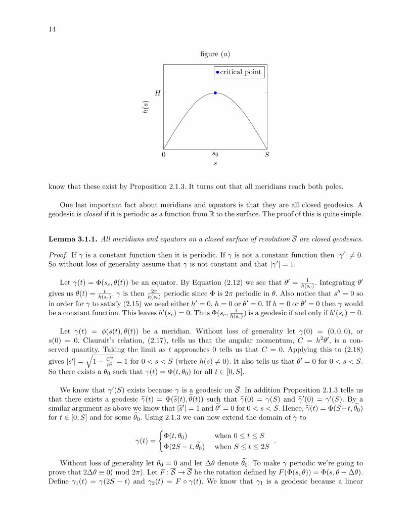
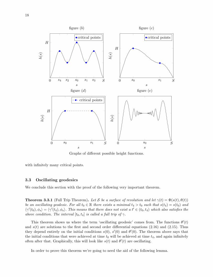
the Geodesic Equations, (2.15) and (2.16), since s′′, θ′′ and h′(sc) are all constantly to 0. It turnsout that all equators share the property that h′(sc) = 0, that is, Φ(sc, θ(t)) is only a geodesic if scis a critical point of h. Critical points of h may look very different. Some examples of critical pointsare s0 on figure (a), s1 on figure (b), s1 on figure (c), any point between s0 and s1 on figure (d),and s0 on figure (e). Figure (a) is below and figures (b) through (e) are on page 18.

If a surface has only one such sc where h′(sc) = 0 then there are no two geometrically distinctequators. In some sense, this is the simplest case for a surface of revolutions. Figure (a) belowillustrates the height function which generates this type of surface.

A meridian on the closed surface of revolution S is a geodesic γ(t) = Φ(s(t), θ(t)) which reachesone or both of the poles. That is to say, there exists a t0 such that γ(t0) = (0, 0, 0) or (0, 0, D). We

14

0 s0 S

H

s

h(s

)

figure (a)

critical point

know that these exist by Proposition 2.1.3. It turns out that all meridians reach both poles.

One last important fact about meridians and equators is that they are all closed geodesics. Ageodesic is closed if it is periodic as a function from R to the surface. The proof of this is quite simple.

Lemma 3.1.1. All meridians and equators on a closed surface of revolution S are closed geodesics.

Proof. If γ is a constant function then it is periodic. If γ is not a constant function then |γ′| 6= 0.So without loss of generality assume that γ is not constant and that |γ′| = 1.

Let γ(t) = Φ(sc, θ(t)) be an equator. By Equation (2.12) we see that θ′ = 1h(sc)

. Integrating θ′

gives us θ(t) = th(sc)

. γ is then 2πh(sc)

periodic since Φ is 2π periodic in θ. Also notice that s′′ = 0 so

in order for γ to satisfy (2.15) we need either h′ = 0, h = 0 or θ′ = 0. If h = 0 or θ′ = 0 then γ wouldbe a constant function. This leaves h′(sc) = 0. Thus Φ(sc,

th(sc)

) is a geodesic if and only if h′(sc) = 0.

Let γ(t) = φ(s(t), θ(t)) be a meridian. Without loss of generality let γ(0) = (0, 0, 0), ors(0) = 0. Claurait’s relation, (2.17), tells us that the angular momentum, C = h2θ′, is a con-served quantity. Taking the limit as t approaches 0 tells us that C = 0. Applying this to (2.18)

gives |s′| =√

1− C2

h2= 1 for 0 < s < S (where h(s) 6= 0). It also tells us that θ′ = 0 for 0 < s < S.

So there exists a θ0 such that γ(t) = Φ(t, θ0) for all t ∈ [0, S].

We know that γ′(S) exists because γ is a geodesic on S. In addition Proposition 2.1.3 tells usthat there exists a geodesic γ(t) = Φ(s(t), θ(t)) such that γ(0) = γ(S) and γ′(0) = γ′(S). By asimilar argument as above we know that |s′| = 1 and θ′ = 0 for 0 < s < S. Hence, γ(t) = Φ(S−t, θ0)for t ∈ [0, S] and for some θ0. Using 2.1.3 we can now extend the domain of γ to

γ(t) =

{Φ(t, θ0) when 0 ≤ t ≤ SΦ(2S − t, θ0) when S ≤ t ≤ 2S

.

Without loss of generality let θ0 = 0 and let ∆θ denote θ0. To make γ periodic we’re going toprove that 2∆θ ≡ 0( mod 2π). Let F : S → S be the rotation defined by F (Φ(s, θ)) = Φ(s, θ + ∆θ).Define γ1(t) = γ(2S − t) and γ2(t) = F ◦ γ(t). We know that γ1 is a geodesic because a linear

15

reparameterization of γ will still satisfy the same second order differential equations. We know thatγ2 is a geodesic because of Proposition 2.1.4.

If t ∈ (0, S) then we can see that

γ1(S + t) = γ(S − t) = Φ(S − t, 0) and

γ2(S + t) = F (γ(S + t)) = Φ(S − t, 2∆θ) .

However, notice that the following chain of equalities also holds for t ∈ (0, S):

γ1(t) = γ(2S − t)= Φ(2S − (2S − t),∆θ) since 2S − t ∈ (S, 2S) for all t ∈ (0, S)

= Φ(t,∆θ)

= F (Φ(t, 0)

= F (γ(t))

= γ2(t) .

Thus by Proposition 2.1.3, γ1 = γ2. Therefore Φ(S− t, 0) = Φ(S− t, 2∆θ) so 2∆θ ≡ 0( mod 2π) asdesired. Without loss of generality let ∆θ = π. We can now extend the domain of γ and define itas:

γ(t) =

Φ(t, 0) when 0 ≤ t ≤ SΦ(2S − t, π) when S ≤ t ≤ 2S

γ(t− 2S) when t > 2S

γ(t+ 2S) when t < 0 .

γ is 2S periodic and our proof is complete.

3.2 Asymptotic geodesics

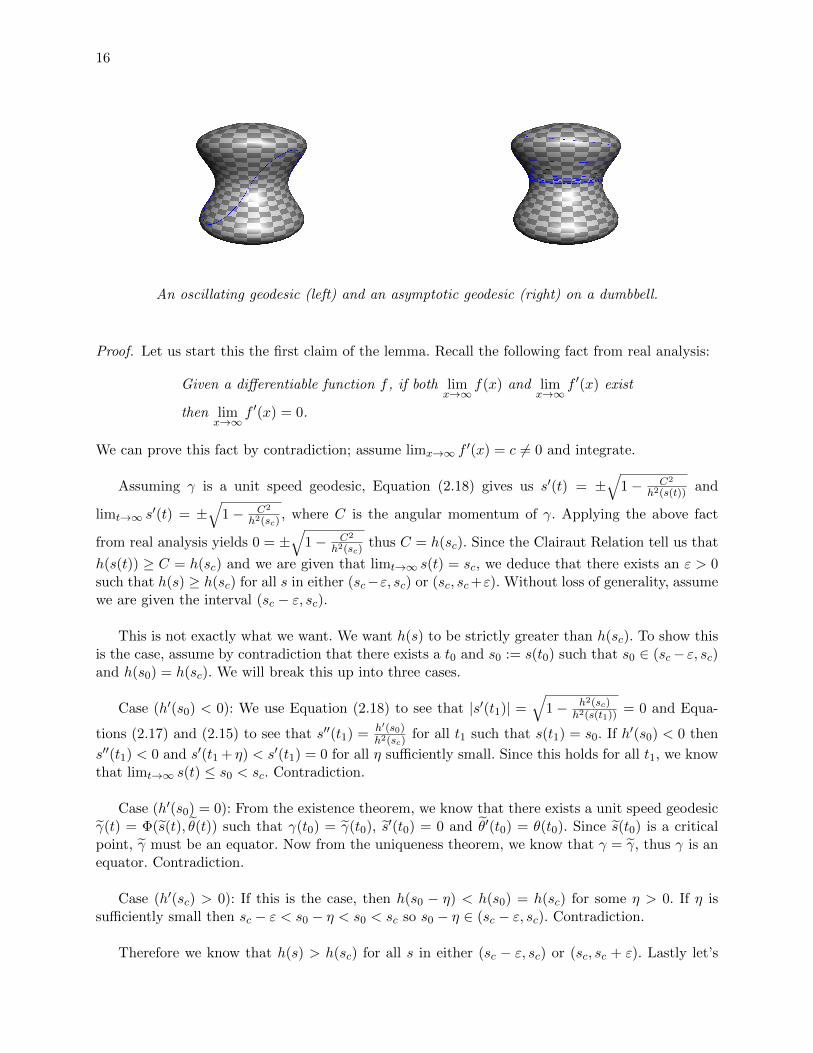
There are two more classes of geodesics on a surfaces of revolution: asymptotic and oscillating. Anasymptotic geodesic is a non-equator geodesic γ(t) = Φ(s(t), θ(t)) where limt→∞ s(t) exists. Wecan think of asymptotic geodesics spiraling away from an equator on an unstable critical point ofh. In Lemma 3.2.1, we will replace the notion of an ‘unstable critical point’ with a more precisedescription.

By definition, an oscillating geodesic is a geodesic which is not asymptotic, not an equator andnot a meridian. As we will see in Theorem 3.3.1, if a geodesic γ(t) = Φ(s(t), θ(t) is oscillating thenboth s(t) and θ′(t) are periodic functions.

All geodesics on a surface of revolution fall into exactly one of these four categories.

Lemma 3.2.1. If γ(t) = Φ(s(t), θ(t)) is an asymptotic geodesic with limt→∞ s(t) = sc then h(sc)is the angular momentum of γ, sc is a critical point of h, and there exists an ε > 0 such thath(s) > h(sc) for all s in either (sc − ε, sc) or (sc, sc + ε). Conversely, if there is a critical point, scof h, and an ε > 0 such that h(s) > h(sc) for all s in either (sc − ε, sc) or (sc, sc + ε), then thereexists an asymptotic geodesic γ(t) = Φ(s(t), θ(t)) with limt→∞ s(t) = sc.

16

An oscillating geodesic (left) and an asymptotic geodesic (right) on a dumbbell.

Proof. Let us start this the first claim of the lemma. Recall the following fact from real analysis:

Given a differentiable function f , if both limx→∞

f(x) and limx→∞

f ′(x) exist

then limx→∞

f ′(x) = 0.

We can prove this fact by contradiction; assume limx→∞ f′(x) = c 6= 0 and integrate.

Assuming γ is a unit speed geodesic, Equation (2.18) gives us s′(t) = ±√

1− C2

h2(s(t))and

limt→∞ s′(t) = ±

√1− C2

h2(sc), where C is the angular momentum of γ. Applying the above fact

from real analysis yields 0 = ±√

1− C2

h2(sc)thus C = h(sc). Since the Clairaut Relation tell us that

h(s(t)) ≥ C = h(sc) and we are given that limt→∞ s(t) = sc, we deduce that there exists an ε > 0such that h(s) ≥ h(sc) for all s in either (sc−ε, sc) or (sc, sc+ε). Without loss of generality, assumewe are given the interval (sc − ε, sc).

This is not exactly what we want. We want h(s) to be strictly greater than h(sc). To show thisis the case, assume by contradiction that there exists a t0 and s0 := s(t0) such that s0 ∈ (sc− ε, sc)and h(s0) = h(sc). We will break this up into three cases.

Case (h′(s0) < 0): We use Equation (2.18) to see that |s′(t1)| =√

1− h2(sc)h2(s(t1))

= 0 and Equa-

tions (2.17) and (2.15) to see that s′′(t1) = h′(s0)h2(sc)

for all t1 such that s(t1) = s0. If h′(s0) < 0 then

s′′(t1) < 0 and s′(t1 + η) < s′(t1) = 0 for all η sufficiently small. Since this holds for all t1, we knowthat limt→∞ s(t) ≤ s0 < sc. Contradiction.

Case (h′(s0) = 0): From the existence theorem, we know that there exists a unit speed geodesicγ(t) = Φ(s(t), θ(t)) such that γ(t0) = γ(t0), s

′(t0) = 0 and θ′(t0) = θ(t0). Since s(t0) is a criticalpoint, γ must be an equator. Now from the uniqueness theorem, we know that γ = γ, thus γ is anequator. Contradiction.

Case (h′(sc) > 0): If this is the case, then h(s0 − η) < h(s0) = h(sc) for some η > 0. If η issufficiently small then sc − ε < s0 − η < s0 < sc so s0 − η ∈ (sc − ε, sc). Contradiction.

Therefore we know that h(s) > h(sc) for all s in either (sc − ε, sc) or (sc, sc + ε). Lastly let’s

17

check that sc is a critical point of h. In case (h′(s0) < 0) we showed that s′′(t) = h′(s(t))h2(sc)

. Since

limt→∞ s(t) and limt→∞ s′(t) exist, we know that limt→∞ s

′′(t) exists and we can apply the factfrom real analysis to see that h′(sc) = h2(sc) limt→∞ s

′′(t) = 0. Hence, sc is a critical point and theproof of the first part of the lemma is complete. Now on to the proof of the converse statement.

Assume without loss of generality that there exists a critical point, sc of h, and an ε > 0 suchthat h(s) > h(sc) for all s ∈ (sc − ε, sc). Pick s0 ∈ (sc − ε, sc). Define the unit speed geodesic

γ(t) = Φ(s(t), θ(t)) by s(0) = s0, θ(0) = 0 and s′(t) =√

1− h2(sc)h2(s(t))

. Let C = h(sc) be its angularmomentum.

Recall that s′ changes sign only when h(s(t)) = C = h(sc). Since s0 ∈ (sc − ε, sc), andh(s) > h(sc) for all s ∈ (sc − ε, sc), we know that s′(t) > 0 for all t > 0. Hence s(t) is a strictlymonotonically increasing function (on the interval [0,∞)). We also know that it is bounded aboveby sc, for if s(t0) = sc then s′(t0) = 0 and h′(s(t0)) = 0 which (by case 2 above) means that γ isan equator. This is not the case, thus s(t) is a strictly monotonically increasing function which isbounded above by sc. We then know that there exists a sc ∈ (s0, sc] such that limt→∞ s(t) = sc.

Since limt→∞ s(t) exists, we also know that limt→∞ s′(t) = limt→∞

√1− h2(sc)

h2(s(t))exists. Applying

the previously stated fact from real analysis tells us that, in fact, limt→∞

√1− h2(sc)

h2(s(t))= 0. Plugging

in sc for limt→∞ s(t) reveals that h(sc) = h(sc). Since sc ∈ (sc − ε, sc] and h(s) > h(sc) for alls ∈ (sc − ε, sc), we see that sc = sc. Therefore γ is a non-equator geodesic where limt→∞ s(t) = scas desired.

The lemma above gives necessary and sufficient conditions for the existence of an asymptoticgeodesic. The following theorem will give only sufficient conditions, but we will be using theseconditions more than the previous ones.

Theorem 3.2.2. Let S be a surface of revolution with height function h : [0, S]→ R. If h has morethan one, but not infinitely many, critical points, then S admits an asymptotic geodesic.

Proof. Let H = max{h(s) : s ∈ [0, S]} and let s0 be a critical point such that h(s0) = H. Since thereare only finitely many critical points we know that every critical point is isolated. This rules out theexample curves found in figures (d) and (e). Let s1 be a critical point such that |s0− s∗| ≥ |s0− s1|for all other critical points s∗. Without loss of generality let s0 < s1. The point s0 is a localmaximum and h′(s) 6= 0 for s ∈ (s0, s1), thus we may conclude that h(s) > h(s1) for all s ∈ (s0, s1).We can see exactly that happening in figures (b) and (c). By Lemma 3.2.1, the fact that s1 is acritical point and that h(s) > h(s1) for all s ∈ (s0, s1) means there that S admits an asymptoticgeodesic γ(t) = Φ(s(t), θ(t)) such that limt→∞ s(t) = s1. This is the conclusion we want; the proofis complete.

Now, it is true that the surface induces by the curve in figure (e) does admit asymptoticgeodesics. And if we worked hard enough we could weaken the conditions on Theorem 3.2.2 so thatit applies to all surfaces with at least two critical points, one of which being isolated. This wouldinclude the curve in figure (e) and exclude the curve in figure (d). However, this is not necessary.Later on, in the results section, we will not need to show the existence of asymptotic geodesics onsurfaces like the one generated by the curve in figure (e). Indeed, we will easily dispose of the case

18

s4 s2 s0 s1 s3

H

0 Ss

h(s

)

figure (b)

critical points

0 s0 s1 S

H

s

h(s

)

figure (c)

critical points

0 s0 s1 S

H

s

h(s

)

figure (d)

critical points

0 s0 Ss

h(s

)

figure (e)

Graphs of different possible height functions.

with infinitely many critical points.

3.3 Oscillating geodesics

We conclude this section with the proof of the following very important theorem.

Theorem 3.3.1 (Full Trip Theorem). Let S be a surface of revolution and let γ(t) = Φ(s(t), θ(t))be an oscillating geodesic. For all t0 ∈ R there exists a minimal t4 > t0 such that s(t4) = s(t0) and〈γ′(t0), φs〉 = 〈γ′(t4), φs〉. This means that there does not exist a t′ ∈ (t0, t4) which also satisfies theabove condition. The interval [t0, t4] is called a full trip of γ.

This theorem shows us where the term ‘oscillating geodesic’ comes from. The functions θ′(t)and s(t) are solutions to the first and second order differential equations (2.16) and (2.15). Thusthey depend entirely on the initial conditions s(0), s′(0) and θ′(0). The theorem above says thatthe initial conditions that were achieved at time t0 will be achieved at time t4, and again infinitelyoften after that. Graphically, this will look like s(t) and θ′(t) are oscillating.

In order to prove this theorem we’re going to need the aid of the following lemma.

19

Lemma 3.3.2. Let S be a surface of revolution. For all oscillating geodesics γ(t) = Φ(s(t), θ(t))on S, and for all t0 ∈ R, there exists a minimal t1 > t0 such that 〈γ′(t1), φθ〉 = |φθ|; that is, γ′(t1)is purely in the θ direction or s′(t1) = 0.

Proof of Lemma. Our curve γ is not an equator, so s(t) is not a constant function. Assume with-out loss of generality that s′(t0 + ε) > 0 for a sufficiently small ε. Now γ is not asymptotic, solimt→∞ s(t) doesn’t exist. But 0 ≤ s(t) ≤ S, so s(t) can’t grow without bound. Thus there exists at > t0 such that s′(t) < 0. By the intermediate value theorem, there exists a t1 ∈ (t0 + ε, t) wheres′(t1) = 0.

The above shows that the set {t > t0 : s′(t) = 0} is nonempty. We now wish to show that thisset has a minimal element. Let t1 = inf{t > t0 : s′(t) = 0}. By continuity, s′(t1) = 0.

I claim that s′′(t1) 6= 0. For if it did, then by Equation (2.15) on page 12, either θ′(t1), h(s(t1))or h′(s(t1)) must equal 0. If h(s(t1)) = 0 then γ(t1) would coincide with one of the poles of S, andγ would be a meridian. If θ′(t1) = 0, then the angular momentum of γ would be 0 and γ would stillbe a meridian. If h′(s(t1)) = 0, then, by the same argument as in Case (h′(s0) = 0) in the poof ofLemma 3.2.1, we see that γ would be an equator. Therefore s′′(t1) 6= 0.

Since s′′(t1) 6= 0 and s′(t1) = 0, we know that there exists an ε > 0 such that s′(t) 6= 0 forall t ∈ (t1 − ε, t1 + ε). This implies that t1 is not a limit point of {t > t0 : s′(t) = 0}, hence,t1 ∈ {t > t0 : s′(t) = 0}. Therefore t1 = min{t > t0 : s′(t) = 0} and is minimal.

Proof of Theorem. Using the above lemma produce a minimal t1 > t0 so that 〈γ′(t1), φθ〉 = |φθ|;that is, γ′(t1) is purely in the θ direction. Let γ(t1) = p. Consider the reflection F : R3 → R3

which preserves the axis of rotation and the point p. F , restricted to S, is an isometry andthus takes geodesics to geodesics. The differential of F at p is an inner product space isometrydF |p : TpS → TpS. It is also a reflection where dF |p(φs) = φs and dF |p(φθ) = −φθ.

Observe that F (γ(t1)) = p and

d

dt

(F ◦ γ(t1 + t)

)∣∣∣t=0

= (F ◦ γ)′(t1)

= dF |p(γ′(t1))

=1

|φθ|dF |p(φθ)

= − φθ|φθ|

= −γ′(t1)

=d

dt

(γ(t1 − t)

)∣∣∣t=0

.

By Proposition 2.1.3 on page 8, γ(t1 + t) = F (γ(t1 − t)). Letting t = t1 − t0 gives

γ(t0 + 2(t1 − t0)) = F (γ(t1 + t1 − t0 − 2t1 + 2t0)) = F (γ(t0)) .

Since F is a reflection, it preserves the s component, so s(t0 + 2(t1 − t0)) = s(t0). Now definet2 = t0 + 2(t1 − t0).

20

From Equation (2.18) on page 13 we see that |s′(t0)| = |s′(t2)|. If s′(t0) = 0, then s′(t0) = s′(t2)and 〈γ′(t0), φs〉 = 〈γ′(t2), φs〉. Let t4 = t2 and we are done.

If s′(t0) 6= 0 then apply Lemma 3.3.2 to produce a t3 > t2 such that s′(t3) = 0. Now lett4 = t2 + 2(t3 − t2) so that s(t4) = s(t2).

Taking the differential of both sides of γ(t1−t) = F ◦γ(t1+t) gives us γ′(t1−t) = −dF (γ′(t1+t)),in particular γ′(t2) = −dF (γ′(t0)). Applying this along with (2.8) gives us the following chain ofequalities:

s′(t2)φs|γ(t2) + θ′(t2)φθ|γ(t2) = γ′(t2)

= −dF (γ′(t0))

= −dF (s′(t0)φs|γ(t0) + θ′(t0)φθ|γ(t0))= −s′(t0)φs|F (γ(t0)) + θ′(t0)φθ|F (γ(t0))

= −s′(t0)φs|γ(t2) + θ′(t0)φθ|γ(t2) .

Now we see that s′(t2) = −s′(t0). Similarly s′(t4) = −s′(t2) or 〈γ′(t0), φs〉 = 〈γ′(t4), φs〉. Theproof is now complete.

Oscillating geodesics are the most interesting for us. What makes them really interesting is thatthey can be uniquely described so easily.

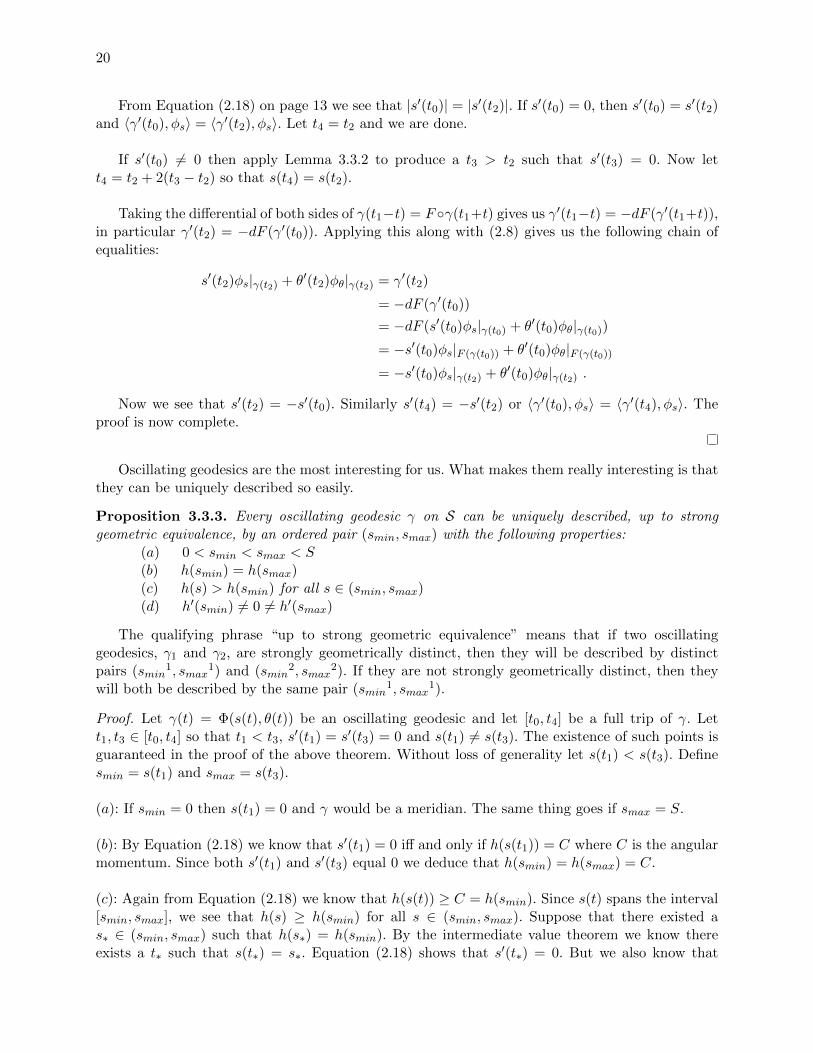
Proposition 3.3.3. Every oscillating geodesic γ on S can be uniquely described, up to stronggeometric equivalence, by an ordered pair (smin, smax) with the following properties:

(a) 0 < smin < smax < S(b) h(smin) = h(smax)(c) h(s) > h(smin) for all s ∈ (smin, smax)(d) h′(smin) 6= 0 6= h′(smax)

The qualifying phrase “up to strong geometric equivalence” means that if two oscillatinggeodesics, γ1 and γ2, are strongly geometrically distinct, then they will be described by distinctpairs (smin

1, smax1) and (smin

2, smax2). If they are not strongly geometrically distinct, then they

will both be described by the same pair (smin1, smax

1).

Proof. Let γ(t) = Φ(s(t), θ(t)) be an oscillating geodesic and let [t0, t4] be a full trip of γ. Lett1, t3 ∈ [t0, t4] so that t1 < t3, s

′(t1) = s′(t3) = 0 and s(t1) 6= s(t3). The existence of such points isguaranteed in the proof of the above theorem. Without loss of generality let s(t1) < s(t3). Definesmin = s(t1) and smax = s(t3).

(a): If smin = 0 then s(t1) = 0 and γ would be a meridian. The same thing goes if smax = S.

(b): By Equation (2.18) we know that s′(t1) = 0 iff and only if h(s(t1)) = C where C is the angularmomentum. Since both s′(t1) and s′(t3) equal 0 we deduce that h(smin) = h(smax) = C.

(c): Again from Equation (2.18) we know that h(s(t)) ≥ C = h(smin). Since s(t) spans the interval[smin, smax], we see that h(s) ≥ h(smin) for all s ∈ (smin, smax). Suppose that there existed as∗ ∈ (smin, smax) such that h(s∗) = h(smin). By the intermediate value theorem we know thereexists a t∗ such that s(t∗) = s∗. Equation (2.18) shows that s′(t∗) = 0. But we also know that

21

h(s) ≥ h(s∗) for all s ∈ (smin, smax). Thus h′(s∗) = 0. Now s(t∗) = s∗, s′(t∗) = 0 and h′(s(t∗)) = 0.

Looking at the differential equations (2.15), (2.16) and recalling the uniqueness theorem 2.1.3, wededuce that s(t) is a constant function and γ is an equator. This is not the case, hence h(s) > h(smin)for all s ∈ (smin, smax).

(d): Assume by contradiction that h′(s(t1)) = 0. Now s(t1) = s1, s′(t1) = 0 and h′(s(t1)) = 0.

Looking at the differential equations (2.15), (2.16) and recalling the uniqueness theorem 2.1.3, wededuce that s(t) is a constant function and γ is an equator. This is not the case, hence h′(smin) 6= 0.A similar argument shows that h′(s(t3)) 6= 0.

We picked the pair (smin, smax) by choosing a full trip of γ. In principle a different full trip mighthave given us a different smin or smax. Let (smin

′, smax′) be another pair for γ. However conditions

(b) applied to (smin, smax) and (c) applied to (smin′, smax

′) mean that [smin′, smax

′] ⊂ [smin, smax].Similarly [smin, smax] ⊂ [smin

′, smax′], thus (smin, smax) is indeed uniquely defined.

Now that we have our map from oscillating geodesics to ordered pairs we need to show that thismap is onto. Let (smin, smax) be a pair satisfying (a) through (d). Define γ(t) = Φ(s(t), θ(t)) bys(0) = smin, s′(0) = 0 and θ(0) = 0 (the initial conditions on θ′(0) come from the Claurait Relation(2.17)). If γ is oscillating then we get a ordered pair (smin

′, smax′) with h(smin

′) = C, the angularmomentum of γ. But we already know that s(0) = smin and s′(0) = 0, so h(smin

′) = h(smin).Now one interval must contain the other. In the above paragraph, we showed that the only waythat would work is if they are equal. All that’s left is to rule out the possibility of γ being asymptotic.

Assume by contradiction that γ is asymptotic with limt→∞ s(t) = sc. By Lemma 3.2.1 we knowthat h′(sc) = 0 and that h(sc) is the angular momentum of γ. However Equation (2.18) tells usthat h(smin) is the angular momentum. If sc < smax then it contradicts condition (c). If sc > smaxthen smax ∈ (smin, sc) and h(s) ≥ h(smax) for all s ∈ (smin, sc) so smax is a critical point of h whichcontradicts condition (d). If sc = smax then smax is again a critical point of h which contradictscondition (d). Therefore γ is indeed an oscillating geodesic and the proof is complete.

We now have a correspondence between strongly geometrically distinct oscillating geodesics andordered pairs satisfying certain properties. This will make our lives much easier. by allowing us todefine functions on the following set, instead of on the space of all oscillating geodesics. Define thefollowing:

Definition.

Γ = {ordered pairs (smin, smax) satisfying (a) through (d) as defined in Proposition 3.3.3}

The set Γ is a subset of R2 and carries the subspace topology. It is, however, entirely one di-mensional. In fact, Γ is the disjoint union of at most countably many open intervals. Here we willprove from this definition, that Γ is locally diffeomorphic to R.

Proposition 3.3.4. Given any point in Γ there exists on open set U⊂Γ containing that point anda diffeomorphism sending V onto U where V is an open subset of R.

Proof. Pick any point (smin, smax) ∈ Γ. Since smin and smax are not critical points of h, theinverse function theorem says there exists a δ > 0 such that h is a diffeomorphism on the in-tervals (smin − δ, smax + δ) and (smax − δ, smax + δ), respectively [7, Theorem C.34]. Let Bδ =

22

[smin − δ, smin + δ] ∪ [smax − δ, smax + δ]. If δ is small enough, we may guarantee that there are nocritical points of h in Bδ. This is because critical points form a closed set.

Let a = min{h(s) : s ∈ [smin+δ, smax−δ]}, b = max{h(s) : s ∈ Bδ} and c = min{h(s) : s ∈ Bδ}.Let x = h(smin) and pick c < y < min{a, b}. Let h−11 and h−12 be the inverses of h on the intervals(smin − δ, smax + δ) and (smax − δ, smax + δ) respectively. Observe that the pair (h−11 (y), h−12 (y))is an element of Γ and that the map y 7→ (h−11 (y), h−12 (y)) is a diffeomorphism onto its image. Allthat’s left to show is that the image of this map is actually an open set in Γ.

Let W = (smin − δ, smax + δ)× (smax − δ, smax + δ) ⊂ R2, V = W ∩ Γ and (z1, z2) ∈ U . Noticethat h(z1) = h(z2) and that h, restricted to the two open intervals, is a diffeomorphism. This mean(z1, z2) = (h−11 (y), h−12 (y)) for some c < y < min{a, b}. Therefore Γ may be locally parameterizedby the real line.

4 Length and rotation of a full trip

4.1 Definition

In this section we are interested in calculating the length and ‘rotation’ of an oscillating geodesicalong a full trip as defined in Theorem 3.3.1. If γ(t) = Φ(s(t), θ(t)) is a unit speed geodesic andI = [t0, t4] a full trip of γ, then the length of γ along I is |t4 − t0| and the rotation along I is|θ(t4)− θ(t0)| (keep in mind that this value may be greater than 2π).

First we will see that, if I and J are two full trips of an oscillating geodesic γ, then the lengthand rotation of γ along I and J will be the same. In fact, we will see that, if any two oscillatinggeodesics γ1 and γ2 are not strongly geometrically distinct, then the length and rotation of γ1 alongany full trip I will always match the length and rotation of γ2 along any full trip J . In other words,length and rotation of an oscillating geodesic depend only on its representation in Γ (see 3.3). Thismakes sense, because there is a one to one correspondence between elements of Γ and oscillatinggeodesics, up to strong geometric equivalence. Using this fact we can view the length and ‘rotation’as well defined functions from Γ to R.

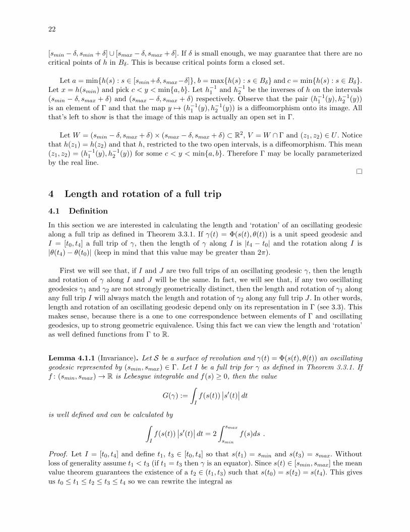
Lemma 4.1.1 (Invariance). Let S be a surface of revolution and γ(t) = Φ(s(t), θ(t)) an oscillatinggeodesic represented by (smin, smax) ∈ Γ. Let I be a full trip for γ as defined in Theorem 3.3.1. Iff : (smin, smax)→ R is Lebesgue integrable and f(s) ≥ 0, then the value

G(γ) :=

∫If(s(t))

∣∣s′(t)∣∣ dtis well defined and can be calculated by∫

If(s(t))

∣∣s′(t)∣∣ dt = 2

∫ smax

smin

f(s)ds .

Proof. Let I = [t0, t4] and define t1, t3 ∈ [t0, t4] so that s(t1) = smin and s(t3) = smax. Withoutloss of generality assume t1 < t3 (if t1 = t3 then γ is an equator). Since s(t) ∈ [smin, smax] the meanvalue theorem guarantees the existence of a t2 ∈ (t1, t3) such that s(t0) = s(t2) = s(t4). This givesus t0 ≤ t1 ≤ t2 ≤ t3 ≤ t4 so we can rewrite the integral as

23

∫If(s(t))

∣∣s′(t)∣∣ dt =4∑i=1

∫ ti

ti−1

f(s(t))∣∣s′(t)∣∣ dt .

Let C be the angular momentum of γ. Since s(t1) = smin we know that s′(t1) = 0 andC = h(smin) = h(smax). Equations (2.18) and (2.17) tell us that s′(t) only changes sign whenh(s(t)) = C; and this occurs only when s(t) = smin or smax.

We can now conclude that s′(t) ≥ 0 for t ∈ [t1, t3] and s′(t) ≤ 0 for t ∈ [t0, t1]∪ [t3, t4]. Using thefundamental theorem of calculus we can define F to be the antiderivative of f . Since s(t0) = s(t2),we see that:

∫ t1

t0

f(s(t))∣∣s′(t)∣∣ dt = −

∫ t1

t0

f(s(t))s′(t)dt

= −∫ t1

t0

(F ◦ s)′ (t)dt

= (F ◦ s) (t0)− (F ◦ s) (t1)

= (F ◦ s) (t2)− (F ◦ s) (t1)

=

∫ t1

t2

f(s(t))s′(t)dt

=

∫ t2

t1

f(s(t))∣∣s′(t)∣∣ dt .

A similar string of calculations shows∫ t3

t2

f(s(t))∣∣s′(t)∣∣ dt =

∫ t4

t3

f(s(t))∣∣s′(t)∣∣ dt ,

and hence ∫If(s(t))

∣∣s′(t)∣∣ dt = 2

∫ t3

t1

f(s(t))∣∣s′(t)∣∣ dt .

Finally we get our desired equality after applying the Fundamental Theorem of Calculus twice:∫ t3

t1

f(s(t))∣∣s′(t)∣∣ dt =

∫ t3

t1

f(s(t))s′(t)dt

= (F ◦ s)(t3)− (F ◦ s)(t1)= F (smax)− F (smin)

=

∫ smax

smin

f(s)ds .

Since this formula does not depend on our choice of I, it stands that G is well defined.

24

Actually, this formula only depends on (smin, smax). One could view this lemma as giving amore geometric view to functions G : Γ→ R of the form

G((smin, smax)) = 2

∫ smax

smin

f(s)ds .

The lemma says that we may calculate G((smin, smax)) by using an oscillating geodesic γ repre-sented by (smin, smax). Having both a geometric and non-geometric expression for the same valuewill enable us to prove many things about these types of functions.

Another useful technique for us will be utilizing Proposition 3.3.4 to locally define G as afunction from some open subset of R to R. Let (smin, smax) ∈ Γ and U⊂Γ be an open set containing(smin, smax). If U is sufficiently small then ψ((smin, smax)) = h(smin) is a diffeomorphism from Uto V ⊂ R. Now define G : V → R by

G(x) :=

∫Ix

f(x, sx(t))|s′x(t)|dt

where γx(t) = Φ(sx(t), θx(t)) is an oscillating geodesics represented by ψ−1(x) = (smin(x), smax(x))and Ix is a full trip of γx. Lemma 4.1.1 says that this function is well defined for any x ∈ Vsuch that f(x, •) is Lebesgue integrable on the interval (smin(x), smax(x)). When it is clear what(smin(x), smax(x)) ought to be, then we may use the abuse of notation and denoteG((smin(x), smax(x)))by G(x) instead of G(x). Other times we may write G(γ) when the choice of geodesic is clear, butintroducing (smin, smax) would be unnecessary to the understanding of the proof.

Our goal is now to define length, L, and rotation, R, as functions from Γ to R. Formally, let Land R be defined by:

L((smin, smax)) := 2

∫ smax

smin

ds√1− h2(smin)

h2(s)

(4.1)

and

R((smin, smax)) := 2

∫ smax

smin

h(smin)ds

h2(s)√

1− h2(smin)h2(s)

. (4.2)

I say formally for two reasons. Firstly, because L and R are defined as improper integrals andwe need to show it converges. Secondly, because in practice we do not write L and R this way. If wehave chosen neighborhoods U⊆Γ and V⊆R such that (smin, smax) 7→ h(smin) is a diffeomorphismfrom U to V , then we may use an abuse of notation and say

L(x) = 2

∫ smax(x)

smin(x)

ds√1− x2

h2(s)

(4.3)

and

R(x) = 2

∫ smax(x)

smin(x)

xds

h2(s)√

1− x2

h2(s)

. (4.4)

Assume anytime we use the notation L(x), R(x), smin(x) or smax(x), that we have already chosenour neighborhoods U and V to allow us to do so.

25

This definition for length and rotation will not be useful unless they have some sort of geometricmeaning. To get a geometric meaning we need to use Lemma 4.1.1 and examine the integrands.

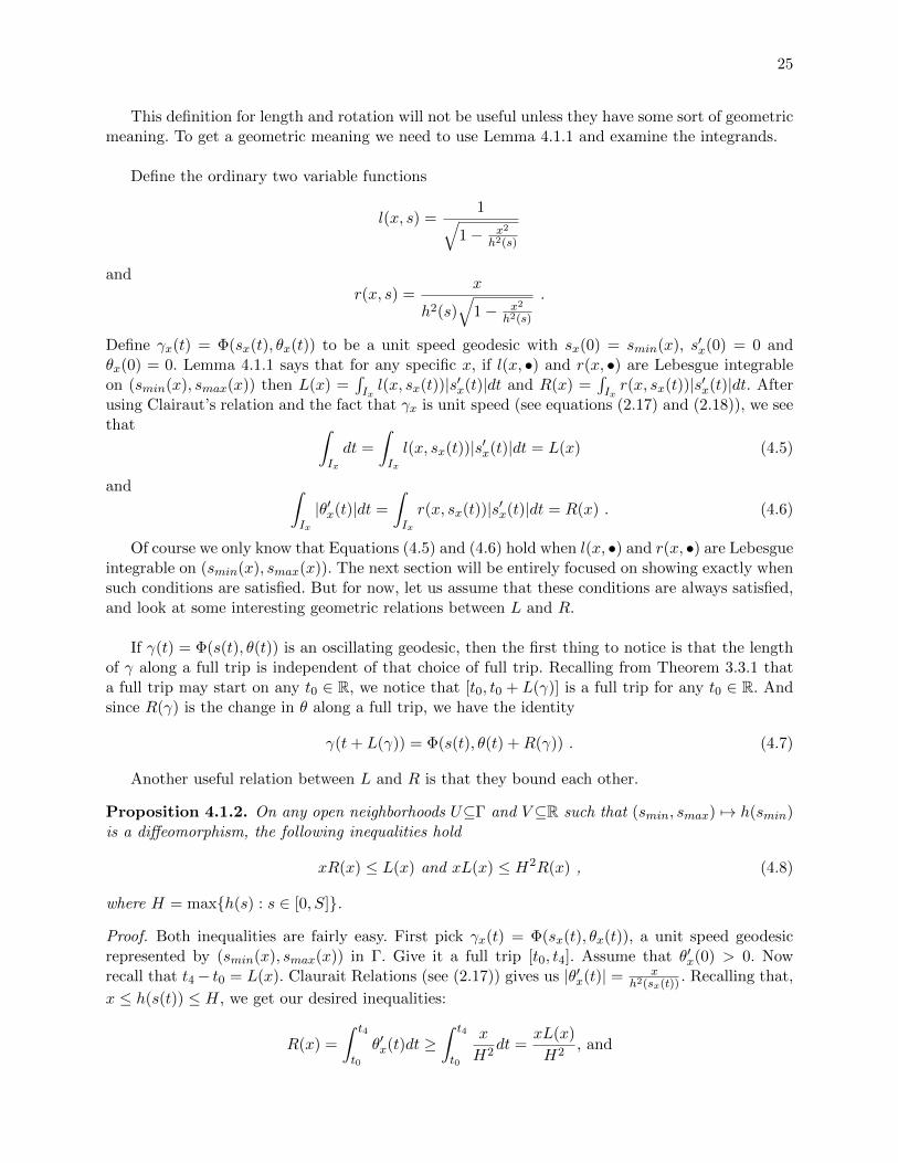
Define the ordinary two variable functions

l(x, s) =1√

1− x2

h2(s)

andr(x, s) =

x

h2(s)√

1− x2

h2(s)

.

Define γx(t) = Φ(sx(t), θx(t)) to be a unit speed geodesic with sx(0) = smin(x), s′x(0) = 0 andθx(0) = 0. Lemma 4.1.1 says that for any specific x, if l(x, •) and r(x, •) are Lebesgue integrableon (smin(x), smax(x)) then L(x) =

∫Ixl(x, sx(t))|s′x(t)|dt and R(x) =

∫Ixr(x, sx(t))|s′x(t)|dt. After

using Clairaut’s relation and the fact that γx is unit speed (see equations (2.17) and (2.18)), we seethat ∫

Ix

dt =

∫Ix

l(x, sx(t))|s′x(t)|dt = L(x) (4.5)

and ∫Ix

|θ′x(t)|dt =

∫Ix

r(x, sx(t))|s′x(t)|dt = R(x) . (4.6)

Of course we only know that Equations (4.5) and (4.6) hold when l(x, •) and r(x, •) are Lebesgueintegrable on (smin(x), smax(x)). The next section will be entirely focused on showing exactly whensuch conditions are satisfied. But for now, let us assume that these conditions are always satisfied,and look at some interesting geometric relations between L and R.

If γ(t) = Φ(s(t), θ(t)) is an oscillating geodesic, then the first thing to notice is that the lengthof γ along a full trip is independent of that choice of full trip. Recalling from Theorem 3.3.1 thata full trip may start on any t0 ∈ R, we notice that [t0, t0 + L(γ)] is a full trip for any t0 ∈ R. Andsince R(γ) is the change in θ along a full trip, we have the identity

γ(t+ L(γ)) = Φ(s(t), θ(t) +R(γ)) . (4.7)

Another useful relation between L and R is that they bound each other.

Proposition 4.1.2. On any open neighborhoods U⊆Γ and V⊆R such that (smin, smax) 7→ h(smin)is a diffeomorphism, the following inequalities hold

xR(x) ≤ L(x) and xL(x) ≤ H2R(x) , (4.8)

where H = max{h(s) : s ∈ [0, S]}.

Proof. Both inequalities are fairly easy. First pick γx(t) = Φ(sx(t), θx(t)), a unit speed geodesicrepresented by (smin(x), smax(x)) in Γ. Give it a full trip [t0, t4]. Assume that θ′x(0) > 0. Nowrecall that t4− t0 = L(x). Claurait Relations (see (2.17)) gives us |θ′x(t)| = x

h2(sx(t)). Recalling that,

x ≤ h(s(t)) ≤ H, we get our desired inequalities:

R(x) =

∫ t4

t0

θ′x(t)dt ≥∫ t4

t0

x

H2dt =

xL(x)

H2, and

26

R(x) =

∫ t4

t0

θ′x(t)dt ≤∫ t4

t0

x

x2dt =

L(x)

x.

To further aid our understanding of what L and R look like, and to see the interplay they havewith the geometry of S, we will prove the following propositions.

Proposition 4.1.3. If the surface of revolution S admits at least one asymptotic geodesic, thenboth L and R are unbounded.

The proof of this proposition is fairly complicated but the main idea is simple. We want toconstruct a sequence of oscillating geodesics, {γn}, which pointwise converge to some asymptoticgeodesic, γ∗. Then we assume by contradiction that |L| ≤ A and see that {γn} converges uniformlyto γ∗ on the closed interval [0, A]. Next we use our assumption to find a contradiction relating toγ∗ being both asymptotic and oscillating.

The first part of the proof, constructing the sequence of oscillating geodesics, is rather difficult.The only other interesting part of the proof is our use of the Arzela−Ascoli Theorem. It states:

Let {fn} be a sequence of functions from X to Y . If the sequence is

uniformly bounded, equicontinuous and X is compact, then we can find a

uniformly convergent subsequence, {fnk}.

Proof. Let γ∗(t) = Φ(s∗(t), θ∗(t)) be an asymptotic geodesic with limt→∞ s∗(t) = s∗max. Defines∗min = inf{s∗(t) : t ∈ R} and without loss of generality, let s∗min < s∗max. Note that the pair(s∗min, s

∗max) does not represent an oscillating geodesic because h′(s∗max) = 0. Without loss of gen-

erality assume that h(s∗(0)) = max{h(s) : s ∈ [s∗min, s∗max]}, s′∗(0) ≥ 0, and define p = γ∗(0).

Step 1:Pick any 0 < ε1 <

12 |s∗max − s∗min| and define hm = min{h(s) : s ∈ [s∗min + ε1, s

∗max − ε1]}. Choose

0 < ε2 < ε1 so that h(s) < hm for all s ∈ [s∗min, s∗min + ε2] ∪ [s∗max − ε2, s∗max].

By the Intermediate Value Theorem there exists a point a0 ∈ [s∗max − ε2, s∗max] such that

h′(a0) < 0. Since h is continuously differentiable, there exists a 0 < ε3 such that h′(s) < 0 for alls ∈ (a0 − ε3, a0 + ε3). Without loss of generality assume (a0 − ε3, a0 + ε3)⊂(s∗max − ε2, s∗max].

Now define a1 = max{s < a0 : h(s) = h(a0)}. We know that a1 ∈ [s∗min, s∗max] because

h(s∗min) < h(a0) and h(a0 − ε3) > h(a0).

By construction, h′(a1) ≥ 0. If h′(a1) 6= 0 then let a1 = a2, a0 = a3 and proceed directly to Step2. If h′(a1) = 0, then choose 0 < ε4 < ε3 such that max{h(s) : s ∈ [a1 − ε4, a1 + ε4]} < max{h(s) :s ∈ [a0 − ε3, a0 + ε3]}. By construction h(a1) < h(a1 + ε4), so we can use the intermediate valuetheorem to find a2 ∈ [a1, a1 + ε4] such that h′(a2) > 0. Finally choose a3 ∈ (a0 − ε3, a0] such thath(a2) = h(a3).

Step 2:The previous highly technical step gave us the points a2 and a3. We constructed these points to

27

have very specific properties. One should notice that a2 < a3, h(a2) = h(a3), h(s) > h(a2) for alls ∈ (a2, a3), and h′(a2) 6= 0 6= h′(a3). These are exactly the conditions needed for (a2, a3) to be in Γ.

Let s1min = a2 and s1max = a3. The pair (s1min, s1max) gives an oscillating geodesic. We need

an entire infinite sequence of oscillating geodesics. To do this, we will have to repeat step 1 in-finitely many times. But before we go back to step 1, we want to place the restriction that thenew ε1 <

12 |s∗max − s1max|. This way we can ensure that limn→∞ s

nmax = s∗max. Now repeat step 1

infinitely many times.

Now that we have {(snmin, snmax)}∞n=1, our sequence of points in Γ, we can construct our sequenceof geodesics. For each n ∈ N, define γn(t) = Φ(sn(t), θn(t)) to be a unit speed oscillating geodesicrepresented by (snmin, s

nmax). Without loss of generality let γn(0) = p and s′n(0) ≥ 0. Let vn = γ′n(0).

Step 3:Assume by contradiction that there exists some real number A, such that |L(γ)| ≤ A for all oscillat-ing geodesics γ. Let Br(0) = {v ∈ TpS : |v| ≤ r}. Consider the exponential map expp : BA(0)→ S.By construction, γn(t) = expp(tvn).

Since expp is a continuous function, it is uniformly continuous on the compact set BA(0). Thusfor all ε > 0 there exists a δ > 0 such that d(expp(u), expp(w)) < ε for all |u − w| < δ withu,w ∈ BA(0). Letting u = tvn and w = t′vn we see that d(γn(t), γn(t′)) < ε for all |t− t′| < δ witht ∈ [0, A]. Since δ had no dependence on n, the sequence {γn} : [0, A]→ S is now an equicontinuousfamily of functions.

Furthermore, recall that S is compact subset of R3. Hence, we can view {γn} as a uniformlybounded, equicontinuous, family of functions. These are precisely the conditions needed to evokethe Arzela-Ascoli Theorem. By doing so we learn that there exists a subsequence, {γnk}, whichconverges uniformly to some function, γ : [0, A] → S defined by γ(t) = Φ(s(t), θ(t)). However, wedo not know if γ is a geodesic yet.

Recall that |vn| = 1, we see that {vnk}⊂B1(0) is an infinite subset of a compact space. Thusthere exists a subsequence which converges to some unit length vector, v∗. Without loss of gener-ality, let limk→∞ vnk = v∗. By continuity of the exponential map we can most the limit throughthe exponential, for any fixed t0, and obtain limk→∞ expp(t0vnk) = expp(t0v∗). Therefore γnk(t)converges pointwise to the geodesic expp(tv∗). Since γnk converges uniformly to γ, we conclude thatγ(t) = expp(tv∗).

Finally we have to show that γ and γ∗ are the same geodesic. To do this I am going to calculatethe angular momentum of γ and deduce that v∗ = γ′∗(0). Let C = inf{h(s(t)) : t ∈ R} be the angu-lar momentum of γ. Recall that for all ε > 0 there exists an N > 0 such that |snmax − s∗max| < ε forall n > N . Thus C ≤ h(s∗max). Also recall that h(sn(t)) ≥ h(s∗max) for all n and for all t ∈ [0, A]. Byassumption, |L(γn)| ≤ A, thus sn([0, A]) = sn(R) and h(sn(t)) ≥ h(s∗max) for all t ∈ R. ThereforeC ≥ h(s∗max). Finally, recall that s′n(0) ≥ 0 and so s′(0) ≥ 0.

We have two geodesics, γ∗ and γ, which cross through the same point, p, having the same an-gular momentum and facing the same direction. We conclude from the Claurait Relation and theexistence and uniqueness theorem that γ = γ∗.

28

Step 4:Since γ is asymptotic, and s′(0) ≥ 0, we know that s(t) ≥ s(0) for all t ∈ [0, A]. Let ε < |s(0)−s1min|.By uniform convergence, there exists an N such that d(γn(t), γ(t)) < ε for all n > N and for allt ∈ [0, A]. Pick any n > N . Using the assumption that L(γn) ≤ A, and the fact that [0, L(γn)] is afull trip of γn (see Equation (4.7)), we deduce that there exists a t′ ∈ [0, A] such that sn(t′) = snmin.Finally observe that |s(t′)− sn(t′)| ≥ |s(0)− snmin| ≥ |s(0)− s1min| > ε. This is a contradiction, andthus L is unbounded.

To be more specific, we showed that L is unbounded near the asymptotic geodesic γ∗. Thismeans that if x = h(s∗max) is the angular momentum of γ∗, then there exists a sequence of oscil-lating geodesics γn with angular momenta xn, such that limn→∞ xn = x and limn→∞ L(γn) = ∞.This is an important clarification because it mentions the angular momentum of γ∗. If we recallthat the angular momentum of γ∗ can not be 0, then we can use the inequality in Proposition 4.1.2to see R(γn) ≥ xnL(γn)

H2 →∞.

The next proposition will show that no matter how L(γ) behaves in general, it will always bebounded for geodesics with sufficiently small angular momenta. This is useful because when wecombine this fact with Proposition 4.8, we see that if R is bounded, then L is bounded.

Proposition 4.1.4. There exists an M > 0 and ε > 0 such that |L(γ)| ≤ M for all oscillatinggeodesics γ with angular momenta less than ε. We say that L is bounded near 0.

The proof of this proposition proceeds similar to that of the previous one, but it is much shorterand easier to follow.

Proof. First, assume by contradiction that L is not bounded near 0; that is, for all N > 0 and allε > 0 there exists an oscillating geodesic γ with angular momentum less than ε such that L(γ) > N .Now, pick any sc which is a critical point of h and let p = Φ(sc, 0). Define γ(t) = expp(tφs) Recallthat γ is a unit speed geodesic and a meridian. Pick A > 0 to be the smallest positive real numberso that γ(A) = Φ(0, 0).

Construct a sequence of unit speed oscillating geodesics {γn} with the following properties:limn→∞ L(γn) = ∞, γn(0) = p, s′n(0) > 0 (note that if s′n(0) = 0 then γn would be an equator),and Cn <

1n where Cn is the angular momentum of γn. Examine the full trip [0, L(γn)]. Define

τn ∈ (0, L(γn)) such that sn(τn) = sn(0) = sc. Since [0, L(γn)] is a full trip, τn is unique.

Splitting up L(γn) into L(γn) = τn+(L(γn)−τn), we see that either τn ≥ L(γn)2 or (L(γn)−τn) ≥

L(γn)2 . The same is true for every n, thus, by the pigeon hole principle, either there exists infinitely

many γj ∈ {γn} such that τj ≥ L(γj)2 or exists infinitely many γj ∈ {γn} such that L(γj)−τj ≥ L(γj)

2 .

Possibly by relabeling indicies, let us say that without loss of generality τn ≥ L(γn)2 for all n.

Notice that expp is a continuous functions so it is uniformly continuous on the compact setBA(0) = {v ∈ TpS : |v| ≤ A}. Hence, for all ε > 0 there exists a δ > 0 such that d(expp(u), expp(w)) <ε for all |u − w| < δ such that u,w ∈ BA(0). Replacing u and w with t0γ

′n(0) and t1γ

′n(0) we see

that d(γn(t0), γn(t1)) < ε for all |t0 − t1| < δ with t ∈ [0, A]. Since δ had no dependence on n, the

29

sequence {γn} : [0, A]→ S is now an equicontinuous family of functions.

Furthermore, recall that S is a compact subset of R3. Hence, we can view {γn} as a uniformlybounded, equicontinuous, family of functions defined on the compact interval [0, A]. These are pre-cisely the conditions needed to evoke the Arzela-Ascoli Theorem. By doing so we learn that thereexists a subsequence, {γnk}, which converges uniformly to some function, γ∗ : [0, A]→ S defined byγ∗(t) = Φ(s∗(t), θ∗(t)). However, we do not know if γ∗ is a geodesic yet.

Recall that |γ′n(0)| = 1, we see that {γ′nk(0)}⊂B1(0) is an infinite subset of a compact space.Thus there exists a subsequence which converges to some unit length vector, v. Without loss of gen-erality, let limk→∞ γ

′nk

(0) = v. By continuity of the exponential map we can push the limit throughthe exponential, for any fixed t0, and obtain limk→∞ expp(t0γ

′nk

(0)) = expp(t0v). Therefore γnk(t)converges pointwise to the geodesic expp(tv). Since γnk converges uniformly to γ∗, we conclude thatγ∗(t) = expp(tv).

Finally we have to show that γ and γ∗ are the same geodesic. Using Equation (2.18) we see that

|s′n(0)| >√

1− 1/n2

h2(sc). Since γ′n(0) = s′n(0)φs + θ′n(0)φθ, we see that limn→∞ γ

′n(0) = φs. Therefore

γ∗ = γ and {γn} : [0, A]→ S uniformly converges to expp(tφs) : [0, A]→ S.

We have almost reached our point of contradiction. Let ε < 12 inf{d(Φ(0, 0),Φ(s, θ)) : s ≥

sc, θ ∈ R}. Now pick N > 0 so that L(γn) ≥ 4A for all n > N . Since {γn} converge uniformlyto γ, we know that there exists an M > 0 such that d(γn(t), γ(t)) < ε for all n > M and allt ∈ [0, A]. In particular, for t = A. However, when n > N then 1

2τn ≥14L(γn) ≥ A. Recalling

that sn(t) ≥ sc for all t ∈ [0, τ ] we see that sn(A) > sc. But this is a contradiction becaused(γ(A), γn(A)) > 1

2 inf{d(Φ(0, 0),Φ(s, θ)) : s ≥ sc, θ ∈ R} > ε. Therefore our assumption waswrong and the proof is complete.

We could almost certainly craft a corollary to this proposition which involves R instead of L.That would imply that R is bounded if and only if L is. It might be a nice relationship betweenL and R, but it would not be useful to this paper, and so we do not pursue the question any further.

Now we have to get back to the question we left earlier; do∫ smax(x)

smin(x)

ds√1− x2

h2(s)

and

∫ smax(x)

smin(x)

xds

h2(s)√

1− x2

h2(s)

converge?

4.2 Integrability

Let’s begin with showing that l is integrable, that is

∫ smax(x)

smin(x)

∣∣∣∣∣∣ ds√1− x2

h2(s)

∣∣∣∣∣∣ <∞ ,

30

for all x such that (smin(x), smax(x)) ∈ Γ. The proof is somewhat technical and keeping track ofsmin and smax can be confusing. To make this easier I have included a labeled graph of “sin(s)”versus “s”. The function sin(s) is the height function, h(s), that we receive when our surface ofrevolutions is a sphere. This is the simplest image to have in mind when thinking of h(s) and itprovides a lot of intuition.

- s

6

h(s)

a

x

b

s0 smax(a)smax(x)smax(b)smin(a)smin(x) smin(b)

H

We are going to start with the proof that the first integral is bounded and then argue that thesecond integral is similar to the first.

Lemma 4.2.1. Let h : [0, S]→ [0, H] be a C∞ function. If h′(0) = 1 = −h′(S) and h(2n)(0) = 0 = h(2n)(S)for all n ≥ 0, then ∫ smax

smin

∣∣∣∣∣∣ 1√1− x2

h2(s)

∣∣∣∣∣∣ ds <∞where x = h(smin) and (smin, smax) ∈ Γ.

Proof. First, notice that 1√1− x2

h2(s)

≥ 0 so we can remove the absolute values. Let (smin, smax) ∈ Γ

and choose a neighborhood U⊆Γ containing (smin, smax) so that (smin, smax) 7→ h(smin) is a dif-feomorphism from U to V⊆R. Let x ∈ V and choose [a, b]⊂V to be any closed interval containingx in its interior. Let U1 and U2 be the sets of all smin and smax in U respectively. This is sayingthat smin ∈ U1 and smax ∈ U2 for all (smin, smax) ∈ U⊂Γ.

Now pick 0 < η′ small enough that smin(y) + η′′ ∈ U1 and smax(y) + η′′ ∈ U2 for all |η′′| < η′

and for all y ∈ [a, b]. Let η = 12η′ and pick 0 < δ < η. We do this to split the integral up into three

31

parts:∫ smax(x)

smin(x)

ds√1− x2

h2(s)

=

∫ smin(x)+δ

smin(x)

ds√1− x2

h2(s)

+

∫ smax(x)−δ

smin(x)+δ

ds√1− x2

h2(s)

+

∫ smax(x)

smax(x)−δ

ds√1− x2

h2(s)

.

We can bound the second part quickly. Notice that 1√1− x2

h2(s)

is continuous whenever h(s) 6= x.

And since s ∈ [smin(x), smax(x)], we know that h(s) = x implies s = smin(x) or s = smax(x). Thusl(x, s) is continuous on the compact set [a, b]× [smin(x)+δ, smax(x)−δ] and a uniform bound exists.Let N = max{l(x, s) : x ∈ [a, b], s ∈ [smin(x) + δ, smax(x)− δ]}.

We can bound the first part using h′m = min{h′(s)|smin(a) ≤ s ≤ smin(b) + η}. Since h has nocritical points in U1, h

′m must be positive. Now observe the following inequalities (see below for

justification):∫ smin(x)+δ

smin(x)

ds√1− x2

h2(s)

=

∫ smin(x)+δ

smin(x)

h2(s)h′(s)ds

h′(s)h2(s)√

1− x2

h2(s)

≤ H2

xh′m

∫ smin(x+δ)

smin(x)

h′(s)xds

h2(s)√

1− x2

h2(s)

(i)

=−H2

xh′m

∫ xx+δ

1

du√1− u2

(ii)

=H2

xh′m

(sin−1(u)

∣∣∣1xx+δ

)=

H2

xh′mcos−1

(x

x+ δ

)≤ H2

ah′mcos−1

(a

a+ δ

)(4.9)

<∞ .

The reader should know that we were able to say smin(x) + δ ≤ smin(x+ δ) in (i) because smin(x)is a local inverse of h and we know that |h′(s)| ≤ 1 due to (2.12). At (ii) we used the change ofvariables u = x

h(s) .

The third integral can be bound using a similar argument as this one. Let

h′M = min{h′(s) : smax(b)− η ≤ s ≤ smax(a)

}and see that after a similar the chain of inequalities we get∫ smax(x)

smax(x)−δ

ds√1− x2

h2(s)

≤ H2

ah′Mcos−1

(a

a+ δ

). (4.10)

Therefore l(x, •) is integrable and∣∣∣∣∣∫ smax(x)

smin(x)l(x, s)ds

∣∣∣∣∣ ≤ 2SN +M cos−1(

a

a+ δ

),

32

where M = H2

a

(1h′m

+ 1h′M

)is a constant which is independent of δ and only depends on a, b and

the function h.

The quantity M cos−1(

aa+δ

)is clearly finite, but moreover, it tends to 0 as δ does. This fact

will be important later. The proof that r is integrable is nearly identical to the above proof so wewill omit it. Now Equations (4.5) and (4.6), along with Propositions 4.8, 4.1.3 and 4.1.4, hold forany (smin, smax) ∈ Γ.

4.3 Continuity

The next thing to do is to prove that L and R are continuous. This turns out to be more difficultthan it sounds. Since L and R are locally defined by an integral we would want to just show thatthey are differentiable by actually computing their derivatives. To do this we would need the LeibnizIntegral Rule: if a(x), b(x) and f(x, t) are all C1 functions and f(x, •) is integrable on (a(x), b(x))then

d

dx

(∫ b(x)

a(x)f(x, t)dt

)=

∫ b(x)

a(x)fx(x, t)dt+ f(x, b(x))b′(x)− f(x, a(x))a′(x) .

However, we can’t apply this rule because the local integral form of L, given by L(x) =∫ smax(x)smin(x)

l(x, s)ds, is actually an improper integral; l(x, s) go to infinity when s = smin(x) or

s = smax(x). If we tried to apply the Leibniz Integral Rule we would get infinities and nonsen-sical terms. For this reason we can’t apply the Leibniz integral rule to L(x) even though smin(x),smax(x) and l(x, s) are all infinitely differentiable where they are defined. The same problem appliesfor R as well.

This problem is solved if we examine the new functions, also defined locally by,

Lδ(x) =

∫ smax(x)−δ

smin(x)+δl(x, s)ds and Rδ(x) =

∫ smax(x)−δ

smin(x)+δr(x, s)ds .

By moving away from the singularities at smin(x) and smax(x) we can apply the Leibniz integralrule to Lδ and Rδ. From this we can show that Lδ and Rδ are smooth. However, as we will latersee, we won’t be able to extend smoothness to L and R. In fact, we will only be able to show thatL and R are continuous using this method.

Lemma 4.3.1 (Smooth Integral Functions). Let a, b : (c0, c1) → R be smooth functions suchthat a(t) ≤ c ≤ b(t) for some c. Let A = {(x, t) ∈ R2 : a(x) ≤ t ≤ b(x) and c0 < x < c1} and letf : A→ R be an integrable function. Then the function

F (x) :=

∫ b(x)

a(x)f(x, t)dt

is smooth if f is smooth.

Proof. First define the function f(x, s) =∫ sc f(x, t)dt and notice that F (x) = f(x, b(x))−f(x, a(x)).

Since a and b are smooth, it stands that if f is smooth then F is smooth.

33

We now wish to prove that f is smooth. Recall the definition of smoothness to be that all partialderivatives exist. Using multi-index notation, f is smooth if and only if ∂αf exists for all n ≥ 0and α = (αn, αn−1, . . . α1) where αj ∈ {s, x} and ∂α = ∂

∂αn· · · ∂

∂α1. To show that ∂f exists we will

break ∂α up into two cases:1) α1 = · · · = αn = x.2) there exists a k ≤ n such that αk+1 = s and α1 = · · · = αk = x and

Proof of Case 1) By the Leibniz integral rule

∂αf(x, s) =∂n

∂xnf(x, s) =

∫ s

c

∂n

∂xnf(x, t)dt ,

which exists because f is smooth.

Proof of Case 2) Set β = (αn, . . . , αk+2). By applying both the fundamental theorem of calculusand the Leibniz integral rule we see

∂αf(x, s) = ∂β∂

∂s

∂k

∂xkf(x, s) = ∂β

∂

∂s

∫ s

c

∂k

∂xkf(x, t)dt = ∂β

∂k

∂xkf(x, s) ,

which exists because f is smooth.

We can apply this lemma to Lδ and Rδ. Observe:Pick any (smin, smax) ∈ Γ, let x = h(smin) and let U , U1, U2, V and [a, b] all have the same defini-tions thay did in the previous section. We know that there exists a c such that s1 < c < s2 for alls1 ∈ U1 and s2 ∈ U2. Let a(x) = smin(x) + δ, b(x) = smax(x)− δ, c0 = a, c1 = b and f equal l andr for Lδ and Rδ respectively. We can clearly see that l(x, s) = 1√

1− x2

h2(s)

and r(x, s) = x

h2(s)

√1− x2

h2(s)

are smooth whenever smin(x) + δ ≤ s ≤ smax(x) − δ. Hence, by the above lemma, both Lδ andRδ are smooth on the open set in Γ corespointing to the interval (a, b), which contains the point(smin, smax). Since (smin, smax) was chosen arbitrarily, it stands that Lδ and Lδ are smooth on allof Γ.

At this point we would want to extend the differentiability of Lδ and Rδ to L and R respectively.To do this we might try to use theorem 7.17 from Rudin which states: if a sequence of differen-tiable functions {fn} converges at a point x0 ∈ [a, b], and if the sequence {f ′n} converges uniformlyon [a, b], then {fn} converges uniformly on [a, b] to the function f and f ′(x) = limn→∞ f

′(x) forany x ∈ [a, b] [10]. We unfortunately can’t apply this theorem because the sequence {L′δ} doesn’tconverge uniformly on any interval. The best we can do is to apply theorem 7.12 in Rudin whichstates: if a sequence of continuous functions {fn} converge uniformly to f then f is continuous [10].Since Lδ and Rδ are continuous all we need to do is show that they converges uniformly to L andR respectively.

Lemma 4.3.2 (Uniform Convergence). The family Lδ uniformly converges to L on every closedinterval in V .

Proof. Let [a, b]⊂V and ε > 0. Pick 0 < η′ small enough that smin(y) +η′′ ∈ U1 and smax(y) +η′′ ∈U2 for all |η′′| < η′ and for all y ∈ [a, b]. Let η = 1

2η′, h′m = min{h′(s)|smin(a) ≤ s ≤ smin(b) + η},

34

h′M = min {h′(s)|smax(b)− η ≤ s ≤ smax(a)} and M = H2

a

(1h′m

+ 1h′M

). Choose 0 < δ small enough

so that δ < η and M cos−1(

aa+δ

)< ε. Now let x ∈ [a, b]. Recalling inequalities (4.9) and (4.10),

observe the following:

|L(x)− Lδ(x)| ≤∫ smin(x)+δ

smin(x)|l(x, s)| ds+

∫ smax(x)

smax(x)−δ|l(x, s)| ds ≤M cos−1

(a

a+ δ

)< ε .

Theorem 4.3.3 (Continuity). The functions L and R are continuous on all of Γ.

Proof. First pick (smin, smax) ∈ Γ. Now choose U⊂Γ containing (smin, smax). Let U be small enoughthat (smin, smax) 7→ h(smin) is a diffeomorphism. Let V be the range of this diffeomorphism andlet h(smin) ∈ [a, b]⊂V . It now sufficies to show that L(x) and R(x) are continuous at on [a, b].

Since Lδ(x) is a family of continuous functions which uniformly converges to L(x) on [a, b]⊂(0, H),we know that L(x) is continuous on [a, b] [10]. This concludes the proof and Step 3.

In the next section we will prove that L and R are differentiable in the special case where s0 isthe only critical point of h and where h′′(s0) < 0.

4.4 Differentiability

In this section we are going to be looking at surfaces with a height function h given which has onlyone critical point. As previously stated, surfaces given by curves of this kind are, in some sense,the easiest to work with. It is not difficult to see that under these conditions, the local definitionof L and R are in fact global definitions.

The reason is that when h has only one critical point, then strongly geometrically distinct oscil-lating geodesics are uniquely described by their angular momentum. This can be seen in the curveon figure (a) on page 14. The opposite can also be seen in the the curve on figure (b) on page 18;two oscillating geodesics γ and γ may be described by smin, smax ∈ (s4, s0) and smin, smax ∈ (s0, s3)yet still have h(smin) = h(smin).

We want to place one more restriction on h. We wan to assume that H = max{h(s) : s ∈[0, S]} = 1. This is acceptable because are always allowed to rescale our surface.

Now, let s0 be the critical point of h. Since h has only one critical point, it looks very similarto sin. This gives us the idea to “force” h to be sin and see what changes. This is the main ideawhich we are taking from Petrics’ thesis (for further discussion, see [9, 3]). Formally, we will makethe substitution h(s) = sin(u) in both of the integrals in the expression

R(x) = 2

∫ s0

smin(x)

xds

h2(s)√

1− x2

h2(s)

+ 2

∫ smax(x)

s0

xds

h2(s)√

1− x2

h2(s)

.

35

The reader might worry whether it is possible to do such a substitution in a smooth way. Butrecall that integration by substitution only calls for our substitution to be continuously differnen-tiable. In general, if g is Lebesgue integrable and ψ continuously differentiable, then the substitutions = ψ(u) is justified and gives us∫ b

ag(s)ds =

∫ ψ−1(b)

ψ−1(a)g(ψ(u))ψ′(u)du .

We can see this by using the fundamental theorem of calculus:∫ b

ag(s)ds = G(b)−G(a)

= (G ◦ ψ)(ψ−1(b))− (G ◦ ψ)(ψ−1(a))

=

∫ ψ−1(b)

ψ−1(a)(G ◦ ψ)−1(u)du

=

∫ ψ−1(b)

ψ−1(a)g(ψ(u))ψ′(u)du .

Notice that g need not be continuous, or even finite at every point.

We want to preform this type of substitution on the two separate integrals. For the first integralwe have a := h−11 (x), b := s0, g(s) := x

h(s)√h2(s)−x2

and ψ(u) := h−11 (sin(u)). For the second integral

we have a := s0, b := h−12 (x), g(s) := x

h(s)√h2(s)−x2

and ψ(u) := h−12 (sin(u)). For convenience, define

F (u) :=

{h−11 (sin(u)) for 0 ≤ u ≤ π

2

h−12 (sin(u)) for π2 ≤ u ≤ π

.

For these two substitutions to be justified, we must ensure that F (u) is continuously differ-entiable on the open intervals (0, π2 ) and (π2 , π). Let f(u) = F ′(u) and observe that f(u) =

cos(u)

h′(h−11 (sin(u)))

for u ∈ [0, π2 ). Similarly f(u) = cos(u)

h′(h−12 (sin(u)))

for u ∈ (π2 , π]. We have sufficient

information to know that f is continuous on (0, π2 ) and (π2 , π). This is because h′, h−11 , h−12 and cosand all smooth functions and h′(h−11 ) only vanished at π/2 (recall that and h′(s) = 0 if and only ifs = s0). In fact, f is smooth on the intervals (0, π2 ) and (π2 , π).

Out of curiosity, let us see what happens at π/2. To find out, we can take a limit:

f(π2−) = lim

u→π2−f(u) = lim

u→π2−

− sin(u)

h′′(h−11 (sin(u)))· h′(h−11 (sin(u)))

cos(u)=−1

h′′(s0)· 1

f(π2−)

.

We obtain a similar expression when calcuating f(π2+). If h′′(s0) 6= 0 then we can rearrange terms

and deduce that

f(u) =

cos(u)

h′(h−11 (sin(u)))

u ∈ [0, π2 )

cos(u)

h′(h−12 (sin(u)))

u ∈ (π2 , π]

1√−h′′(s0)

u = π2

36

is a continuous function. In this case we could have left R(x) as one integral and used only onesubstitution. However if h′′(s0) = 0 then we are left with three options: f(π2

−) = 0, 0 < f(π2−) <∞,

and f(π2−) =∞. If f(π2

−) is finite then −1h′′(s0)

1f(π

2−)

is infinite and we are left with a contradiction.

If f(π2−) = 0 then −1

h′′(s0)1

f(π2−)

is infinite and we are left with a contradiction. Finally if f(π2−) =∞

then −1h′′(s0)

1f(π

2−)

is in indeterminate form and we are possibly not left with a contradiction. Since

this is the only remaining option, we assume that f(π2 ) =∞ if h′′(s0) = 0.

Now that we know our substitutions are possible, we can apply it to R(x). For the first integral,∫ s0

h−11 (x)

xds

h(s)√h2(s)− x2

=

∫ π2

sin−1(x)

xf(u)du

sin(u)√

sin2(u)− x2where sin(u) = h(s) and f(u)du = ds

=

∫ π2

y

sin(y)f(u)du

sin(u)√

sin2(u)− sin2(y)where y = sin−1(x) .

Similarly, for the second integral we obtain∫ h−12 (x)

s0

xds

h(s)√h2(s)− x2

=

∫ π−y

π2

sin(y)f(u)du

sin(u)√

sin2(u)− sin2(y).

We go further by making the second integral appear like the first∫ π−y

π2

sin(y)f(u)du

sin(u)√

sin2(u)− sin2(y)=

∫ π2

π−y

sin(y)f(u)du

sin(−u)√

sin2(−u)− sin2(y)

=

∫ π2

y

− sin(y)f(π − u)du

sin(u− π)√

sin2(u− π)− sin2(y)replace u with π − u

=

∫ π2

y

sin(y)f(π − u)du

sin(u)√

sin2(u)− sin2(y).

We can now bring the two integrals together to get

R(x) = 2

∫ π2

y

sin(y)f1(u)du

sin(u)√

sin2(u)− sin2(y)

where f1(u) = f(u) + f(π − u). This has eliminated one of the y’s in the bounds of integration.

In order to move further, we will use a very clever substitution. Define the diffeomorphismv : [0, π/2] → [y, π/2] so that u = tan−1

(tan(y) sec(v)

)and du = tan(y) tan(v) sec(v)

1+tan2(y) sec2(v)dv. It is easy to

see that this is indeed a diffeomorphism. The purpose of this is to eliminate the other y in thebounds of integration.

Since v is a diffeomorphism, we can define f2(v) := f1(tan−1

(tan(y) sec(v)

))= f1(u). Lastly

we calculate sin(u) = sin(tan−1 (tan(y) sec(v))

)= tan(y) sec(v)√

1+tan2(y) sec2(v). Now let’s see just how much

this simplifies the integrand:

37

sin(y)du

sin(u)√

sin2(u)− sin2(y)=

sin(y)

tan(y) sec(v)√1+tan2(y) sec2(v)

√tan2(y) sec2(v)

1+tan2(y) sec2(v)− sin2(y)

· tan(y) tan(v) sec(v)dv

1 + tan2(y) sec2(v)

=sin(y) tan(v)dv√

tan2(y) sec2(v)− sin2(y)− tan2(y) sec2(v) sin2(y)

=sin(y) tan(v)dv√

tan2(y) sec2(v)(1− sin2(y))− sin2(y)

=sin(y) tan(v)dv√

sin2(y) sec2(v)− sin2(y)

= dv .

The integrand becomes nearly trivial! We plug this into the integral and we see

∫ π/2

y

sin(y)f1(u)du

sin(u)√

sin2(u)− sin2(y)=

∫ π/2

0f2(v)dv =

∫ π/2

0f1(tan−1

(tan(y) sec(v)

))dv ,

and

R(x) = 2

∫ π/2

0f1

(tan−1

(x sec(v)√

1− x2

))dv .

This is just what we wanted. We are now ready to use the Lebesgue Dominated ConvergenceTheorem. It states:

Let {gn} be real valeud sequence of measurable functions which converge

pointwise to some f . If |gn(x)| ≤ G(x) for some Lebesgue integrable function G,

then g is integrable and limn→∞

∫gn =

∫g.

We’re trying to pass a derivative, with respect to x, through the integral so our sequence of

functions is the difference quotients of f1

(tan−1

(x sec(v)√1−x2

)). This function is differentiable in x

when v ∈ (0, π/2), so the sequence converges pointwise.

Now we need to check that f1

(tan−1

(x sec(•)√1−x2

))is dominated by an integrable function. If

h′′(s0) < 0 then

f(u) =

cos(u)

h′(h−11 (sin(u)))

u ∈ [0, π2 )

cos(u)

h′(h−12 (sin(u)))

u ∈ (π2 , π]

1√−h′′(s0)

u = π2

is a continuous function. Because it is defined on the closed interval [0, π], there must exists somepositive constant M such that |f(u)| ≤M for all u ∈ [0, π]. Recalling that f1(u) = f(u)+f(π−2) wesee that |f1(u)| ≤ 2M . The constant function 2M is certainly Lebesgue integrable on the boundedinterval (0, π/2), Therefore we can apply the Lesbege Dominated Convergence Theorem and get

R′(x) = 2

∫ π/2

0

d

dx

(f1

(tan−1

(x sec(v)√

1− x2

)))dv .

38

We do not know how to show R is differentiable if h′′(s0) = 0, however it will not be necessary todo so.

Observe that tan−1(x sec(v)√1−x2

)is a smooth function in x for all x ∈ (0, 1). Also observe that

f1(u) = f(u) + f(π − u) and f is smooth whenever u 6= π2 . This means that if we wish to pass

another k derivatives through the integral, we need only show that limu→π2f (k)(u) exists and is

finite. We would then bound the kth derivative difference quotients of f by a constant, use theLebesgue Dominated Convergence Theorem, and conclude that R is k times differentiable.

We will not however be proving that R is smooth. In stead we will prove the following theorem.

Theorem 4.4.1. Let S be a surface of revolution with height function h where max{h(s) : s ∈[0, S]} = 1. If s0 is the only critical point of h, and if h′′(s0) < 0, then both R and L are differentiablefunctions. Furthermore, if R ∈ Ck then L ∈ Ck.

Proof. Because h has only one critical point, we know that the local integral definitions of R andL, are actually a global definitions. Hence we can refer to R(x) and L(x) without ambiguity.

The function R(x) is differentiable by the above argument. Now recall our relation between γ,R, and L that we get from Equation (4.7):

γ(t+ L(γ)) = Φ(s(t), θ(t) +R(γ)) .

This holds for any oscillating geodesic γ(t) = Φ(s(t), θ(t)). In particular, for the family of geodesicswe are about to construct.

Pick p = Φ(s0, 0) and let vx ∈ TpS be defined by vx = φθ|φθ|x+ φs

|φs|√

1− x2. Define expp(tvx) =

γx(t) = Φ(sx(t), θx(t)). Notice that γx is unit speed and that x is the angular momentum of γx.Since θx(t) is a solution to a second order differential equation, it smoothly depends on its initialconditions. Thus θ(x, t) := θx(t) is a smooth function of both x and t for all x ∈ (0, 1) and t ∈ R.

Now we look at Equation (4.7) as a relation between θ(x, t), R(x) and L(x) and we see

θ(x, t) +R(x) = θ(x, t+ L(x)) .

Differentiating both sides gives us

∂θ

∂x

∣∣∣(x,t)

+R′(x) =∂θ

∂x

∣∣∣(x,t+L(x))

+∂θ

∂t

∣∣∣(x,t+L(x))

L′(x) ,

and rearranging terms yields

L′(x) =R′(x) + ∂θ

∂x(x, t)− ∂θ∂x(x, t+ L(x))

∂θ∂t (x, t+ L(x))

.

Recall that |∂θ∂t | > 0. Hence, if we restrict 0 < x < 1, then L(x) is continuously differentiable.In general if we assume that R(x) is k times differentiable then, for all n < k,

L(n+1)(x) =∂n

∂xn

(R′(x) + ∂θ

∂x(x, t)− ∂θ∂x(x, t+ L(x))

∂θ∂t (x, t+ L(x))

)=F (t, x, L(x), . . . , L(n)(x), R′(x), . . . , R(n+1)(x))(

∂θ∂t (x, t+ L(x))

)2n ,

for some smooth function F of 2(n+1) variables. Therefore, by induction, L is k times differentiable.

39

5 Results

5.1 Rational points

In this section we complete Step 4 of our proof strategy.

Theorem 5.1.1 (Rational points). Let S be a surface of revolution with max height H. For everydistinct x such that (smin(x), smax(x)) ∈ Γ and R((smin(x), smax(x)) ∈ 2πQ, there is a stronglygeometrically distinct closed geodesic with angular momentum x.

Proof. Recall formula (4.7):

γ(t+ L(γ)) = Φ(s(t), θ(t) +R(γ)) .

Replacing t with t+ L(γ) gives us

γ(t+ 2L(γ)) = Φ(s(t), θ(t) + 2R(γ)) ,

and by induction we get the general formula

γ(t+ kL(γ)) = Φ(s(t), θ(t) + kR(γ)) . (5.1)

Now let’s examine what happens when R(γ) is rational multiple of 2π, that is R(γ) = 2π nm

where n and m are positive coprime integers. Applying the previous formula gives us

γ(t+mL(γ)) = Φ(s(t), θ(t) +mR(γ)) = Φ(s(t), θ(t) + 2πn) = Φ(s(t), θ(t)) = γ(t) .

Hence, if R(γ) = 2π nm , then γ is periodic with period mL(γ). Lemma 2.3.1 tells us that if two

geodesics have different angular momenta then there is no rotation taking one to the other. There-fore, for every distinct x such that (smin(x), smax(x)) ∈ Γ and R((smin(x), smax(x)) ∈ 2πQ, thereis a strongly geometrically distinct closed geodesic with angular momentum x.

5.2 Infinitude of closed geodesics

In this section we prove the main result of this paper: that on any closed, simply connected surfaceof revolution, there are infinitely many closed strongly geometrically distinct geodesics. We willbreak this up into three cases: the height function h has infinity many critical points, it has finitelymany but more than one, and there is one unique critical point. The last case has two subcases:h′′ = 0 at the critical point, h′′ 6 0 at the critical point.

Theorem 5.2.1. Every closed simply connected surface of revolution has infinitely many stronglygeometrically distinct closed geodesics.

Proof. Case 1: The number of critical points is infinite.For this case we refer to Lemma 3.1.1 which states that all equators are closed geodesics. This, com-bined with the fact that for any critical point sc, the function Φ(sc,

th(sc)

) is an equator, means thatthere are infinitely many distinct closed geodesics. We know that they are strongly geometricallydistinct because rotations do not affect the s coordinate. In other words, for any two distinct criticalpoints s0 and s1, there is no rotation sending the equator Φ(s0,

th(sc)

) to the equator Φ(s1,t

h(sc)).

Therefore there are infinitely many strongly geometrically distinct closed geodesics.

40

Case 2: The number of critical points is less than infinity but more than one.This case satisfies the conditions of Theorem 3.2.2 which gives us the existence of at least oneasymptotic geodesic. Now we use Proposition 4.1.3 to see that R is unbounded. Since R is un-bounded, it is non-constant. Any non-constant continuous real valued function assumes infinitelymany points in 2πQ. By Theorem 5.1.1 this corresponds to infinitely many strongly geometricallydistinct closed geodesics. We have now finished Step 6.

Case 3: The point s0 is the only critical point of h.When this is the case we have the ability to express R is a better form. Without loss of generalitywe can let max{h(s) : s ∈ [0, S]} = 1 by rescaling. Now, just as we did in Section 4.4, we canexpress R as a function of x and write

R(x) = 2

∫ π/2

0f1

(tan−1

(x sec(v)√

1− x2

))dv .

If R(x) is not a constant function then, by the same argument as the on in case 2, there are in-finitely many strongly geometrically distinct closed geodesics. If R(x) is a constant function, thenR(y) = limx→z R(x) for all y ∈ (0, 1) and z ∈ [0, 1].

The Lebesgue Dominated Convergence Theorem will allow us to pull the limit inside the integral,

but only if f1

(tan−1

(x sec(•)√1−x2

))is dominated by a function, integrable on (0, π/2), for all x ∈ [0, ε).

In the proof of Theorem 4.4.1 we see that this condition is upheld when h′′(s0) < 0. So assume, fornow at least, that h′′(s0) < 0 so that we can pull the limit through the integral. We are also allowedto pull the limit through both f1 and tan−1 because they are uniformly continuous; f1 is now acontinuous function defined on the compact interval [0, π/2] and tan−1 is uniformly continuous onall of R. Hence we can pull the limit through all our obstacles and reveal

limx→0

R(x) = limx→0

2

∫ π/2

0f1

(tan−1

(x sec(v)√

1− x2

))dv

= 2

∫ π/2

0f1

(tan−1

(limx→0

x sec(v)√1− x2

))dv

= 2

∫ π/2

0dvf1 (0)

= π(f(0) + f(π))

= π

(cos(0)

h′(h−11 (sin(0))

) +cos(π)

h′(h−12 (sin(π))

))

= π

(1

h′ (0)− 1

h′ (S)

)= 2π .

This value is certainly in 2πQ, therefore all oscillating geodesics on S are closed. We will shortlysee that this concludes Step 5.

Now wee look at the case when h′′(s0) ≥ 0. If h′′(s0) > 0 then s0 would be a local minimum.Since h(0) = 0 = h(S) and h(s) ≥ 0 we know that this is impossible. Thus assume that h′′(s0) = 0.

41

For this case let us take the pointwise limit as x tends towards 1 of our integrand. This shows

limx→1

f1

(tan−1

(x sec(v)√

1− x2

))= f1

(tan−1

(limx→1

x sec(v)√1− x2

))= f1(

π

2)

= 2f(π

2)

=2√

−h′′(s0)=∞ .

Again, this is only pointwise converge, but if we restrict c to any compact interval [a, b]⊂(0, π/2),then we get uniform convergence. This means that for all N > 0 there exists a δ > 0 such that

f1

(tan−1

(x sec(v)√1−x2

))> N for all x ∈ (1 − δ, 1) and for all v ∈ [a, b]. Calculating R(x) when

x ∈ (1− δ, 1) shows us

R(x) =

∫ π/2

0f1

(tan−1

(x sec(v)√

1− x2

))dv ≥

∫ b

af1

(tan−1

(x sec(v)√

1− x2

))dv ≥ N |b− a| .

Since N is arbitrary and does not depend on a or b, we see that R is unbounded. Therefore R isnot constant and we have a contradiction.

We have completed the proof of our main theorem, and thus completed Step 7 our proof strat-egy. Let us now look at an interesting corollary.

Corollary 5.2.2. If max{h(s) : s ∈ [0, S]} = 1, s0 is the only critical point of h, and if R is aconstant function, then R ≡ 2π and h′′(s0) = −1.

Proof. The first claim was proven in the theorem above. The following calculation proves the secondclaim:

2π = limx→1

R(x) =2π√−h′′(s0)

.

5.3 Counting

In this sections section we aim to count the number of strongly geometrically distinct closedgeodesics whose total length is less than `. We will call this function N(`). This will be an analogue

to Hingston’s theorem. We prove N(`) grows at least as fast as `2

log ` .

Theorem 5.3.1. Let S be a closed surface of revolution with height function h. Let N(`) denotethe number of strongly geometrically distinct closed geodesics on S with length less than `. Thereexist positive real constants C and `0 such that

N(`) ≥ C `2

log `

for all ` > `0.

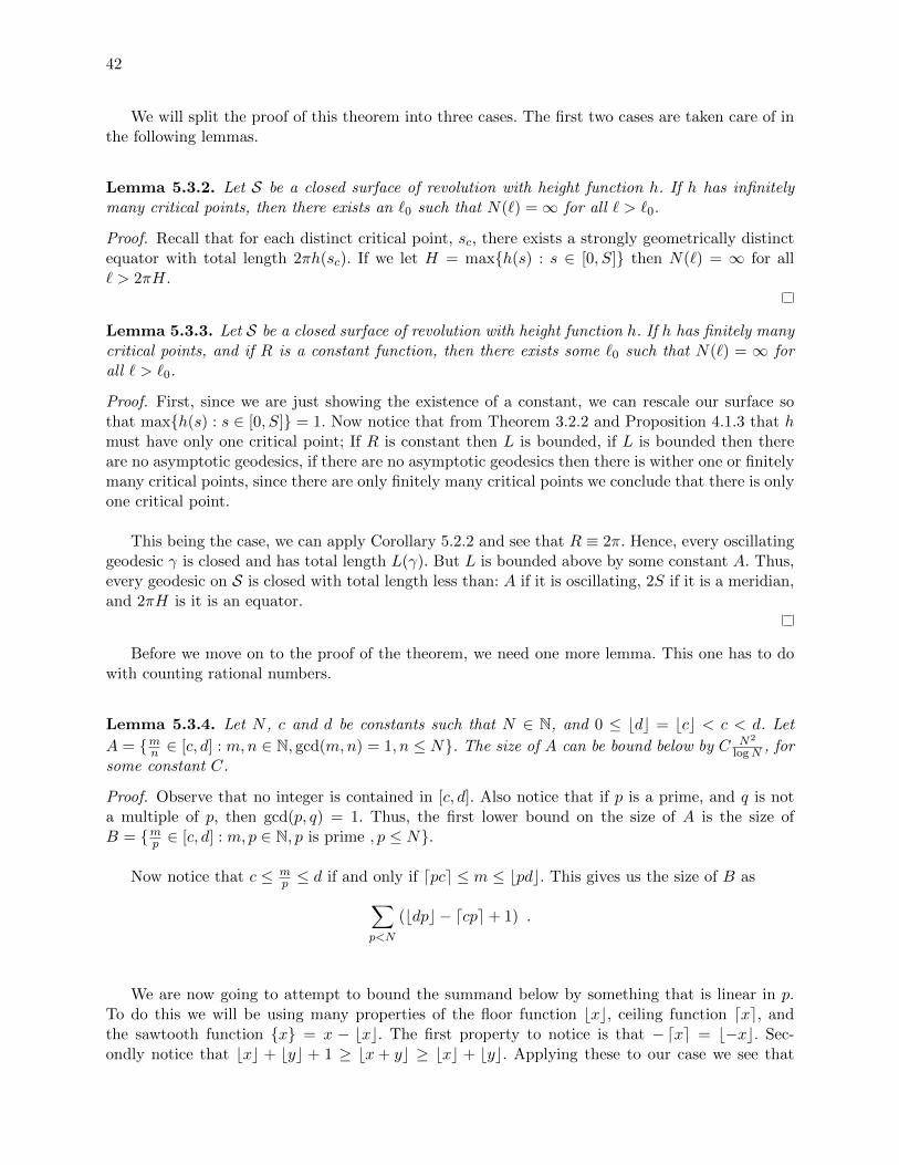
42

We will split the proof of this theorem into three cases. The first two cases are taken care of inthe following lemmas.

Lemma 5.3.2. Let S be a closed surface of revolution with height function h. If h has infinitelymany critical points, then there exists an `0 such that N(`) =∞ for all ` > `0.

Proof. Recall that for each distinct critical point, sc, there exists a strongly geometrically distinctequator with total length 2πh(sc). If we let H = max{h(s) : s ∈ [0, S]} then N(`) = ∞ for all` > 2πH.

Lemma 5.3.3. Let S be a closed surface of revolution with height function h. If h has finitely manycritical points, and if R is a constant function, then there exists some `0 such that N(`) = ∞ forall ` > `0.

Proof. First, since we are just showing the existence of a constant, we can rescale our surface sothat max{h(s) : s ∈ [0, S]} = 1. Now notice that from Theorem 3.2.2 and Proposition 4.1.3 that hmust have only one critical point; If R is constant then L is bounded, if L is bounded then thereare no asymptotic geodesics, if there are no asymptotic geodesics then there is wither one or finitelymany critical points, since there are only finitely many critical points we conclude that there is onlyone critical point.

This being the case, we can apply Corollary 5.2.2 and see that R ≡ 2π. Hence, every oscillatinggeodesic γ is closed and has total length L(γ). But L is bounded above by some constant A. Thus,every geodesic on S is closed with total length less than: A if it is oscillating, 2S if it is a meridian,and 2πH is it is an equator.

Before we move on to the proof of the theorem, we need one more lemma. This one has to dowith counting rational numbers.

Lemma 5.3.4. Let N , c and d be constants such that N ∈ N, and 0 ≤ bdc = bcc < c < d. Let

A = {mn ∈ [c, d] : m,n ∈ N, gcd(m,n) = 1, n ≤ N}. The size of A can be bound below by C N2

logN , forsome constant C.

Proof. Observe that no integer is contained in [c, d]. Also notice that if p is a prime, and q is nota multiple of p, then gcd(p, q) = 1. Thus, the first lower bound on the size of A is the size ofB = {mp ∈ [c, d] : m, p ∈ N, p is prime , p ≤ N}.

Now notice that c ≤ mp ≤ d if and only if dpce ≤ m ≤ bpdc. This gives us the size of B as∑

p<N

(bdpc − dcpe+ 1) .

We are now going to attempt to bound the summand below by something that is linear in p.To do this we will be using many properties of the floor function bxc, ceiling function dxe, andthe sawtooth function {x} = x − bxc. The first property to notice is that −dxe = b−xc. Sec-ondly notice that bxc + byc + 1 ≥ bx+ yc ≥ bxc + byc. Applying these to our case we see that

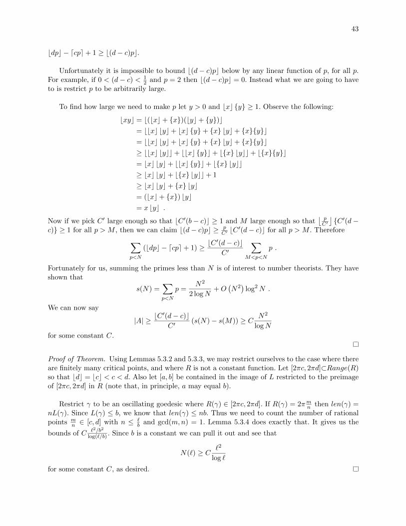
43

bdpc − dcpe+ 1 ≥ b(d− c)pc.

Unfortunately it is impossible to bound b(d− c)pc below by any linear function of p, for all p.For example, if 0 < (d− c) < 1

2 and p = 2 then b(d− c)pc = 0. Instead what we are going to haveto is restrict p to be arbitrarily large.

To find how large we need to make p let y > 0 and bxc {y} ≥ 1. Observe the following:

bxyc = b(bxc+ {x})(byc+ {y})c= bbxc byc+ bxc {y}+ {x} byc+ {x}{y}c= bbxc byc+ bxc {y}+ {x} byc+ {x}{y}c≥ bbxc bycc+ bbxc {y}c+ b{x} bycc+ b{x}{y}c= bxc byc+ bbxc {y}c+ b{x} bycc≥ bxc byc+ b{x} bycc+ 1

≥ bxc byc+ {x} byc= (bxc+ {x}) byc= x byc .

Now if we pick C ′ large enough so that bC ′(b− c)c ≥ 1 and M large enough so that⌊ pC′

⌋{C ′(d−

c)} ≥ 1 for all p > M , then we can claim b(d− c)pc ≥ pC′ bC

′(d− c)c for all p > M . Therefore∑p<N

(bdpc − dcpe+ 1) ≥ bC′(d− c)cC ′

∑M<p<N

p .

Fortunately for us, summing the primes less than N is of interest to number theorists. They haveshown that

s(N) =∑p<N

p =N2

2 logN+O

(N2)

log2N .

We can now say

|A| ≥ bC′(d− c)cC ′

(s(N)− s(M)) ≥ C N2

logN

for some constant C.

Proof of Theorem. Using Lemmas 5.3.2 and 5.3.3, we may restrict ourselves to the case where thereare finitely many critical points, and where R is not a constant function. Let [2πc, 2πd]⊂Range(R)so that bdc = bcc < c < d. Also let [a, b] be contained in the image of L restricted to the preimageof [2πc, 2πd] in R (note that, in principle, a may equal b).

Restrict γ to be an oscillating goedesic where R(γ) ∈ [2πc, 2πd]. If R(γ) = 2πmn then len(γ) =nL(γ). Since L(γ) ≤ b, we know that len(γ) ≤ nb. Thus we need to count the number of rationalpoints m

n ∈ [c, d] with n ≤ `b and gcd(m,n) = 1. Lemma 5.3.4 does exactly that. It gives us the

bounds of C `2/b2

log(`/b) . Since b is a constant we can pull it out and see that

N(`) ≥ C `2

log `

for some constant C, as desired.

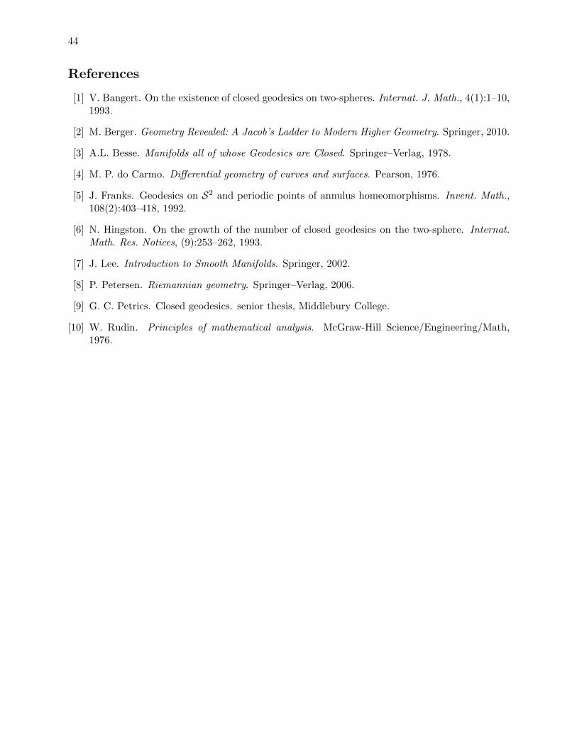
44

References

[1] V. Bangert. On the existence of closed geodesics on two-spheres. Internat. J. Math., 4(1):1–10,1993.

[2] M. Berger. Geometry Revealed: A Jacob’s Ladder to Modern Higher Geometry. Springer, 2010.

[3] A.L. Besse. Manifolds all of whose Geodesics are Closed. Springer–Verlag, 1978.

[4] M. P. do Carmo. Differential geometry of curves and surfaces. Pearson, 1976.

[5] J. Franks. Geodesics on S2 and periodic points of annulus homeomorphisms. Invent. Math.,108(2):403–418, 1992.

[6] N. Hingston. On the growth of the number of closed geodesics on the two-sphere. Internat.Math. Res. Notices, (9):253–262, 1993.

[7] J. Lee. Introduction to Smooth Manifolds. Springer, 2002.

[8] P. Petersen. Riemannian geometry. Springer–Verlag, 2006.

[9] G. C. Petrics. Closed geodesics. senior thesis, Middlebury College.

[10] W. Rudin. Principles of mathematical analysis. McGraw-Hill Science/Engineering/Math,1976.