geodesics in random geometry - people
TRANSCRIPT
Geodesics in random geometry
Jean-François Le Gall
Université Paris-Saclay
Oxford Discrete Mathematics and Probability seminar
Jean-François Le Gall (Univ. Paris-Saclay) Geodesics in random geometry Oxford seminar 1 / 34
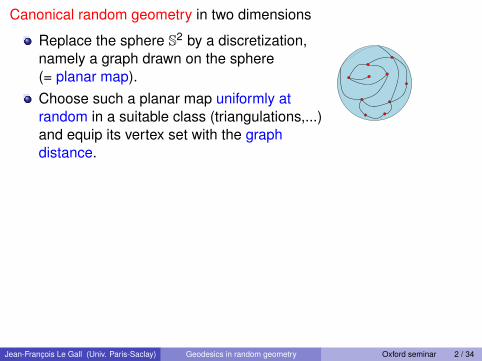
Canonical random geometry in two dimensions
Replace the sphere S2 by a discretization,namely a graph drawn on the sphere(= planar map).Choose such a planar map uniformly atrandom in a suitable class (triangulations,...)and equip its vertex set with the graphdistance.
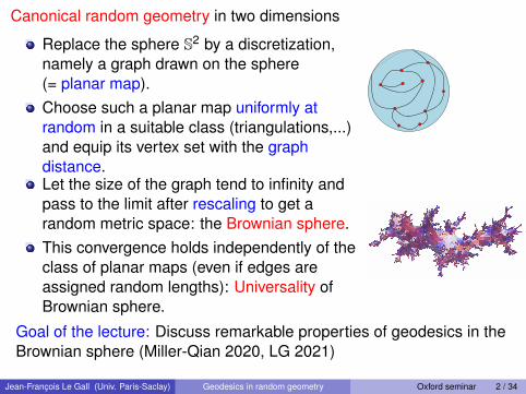
Let the size of the graph tend to infinity andpass to the limit after rescaling to get arandom metric space: the Brownian sphere.This convergence holds independently of theclass of planar maps (even if edges areassigned random lengths): Universality ofBrownian sphere.
Goal of the lecture: Discuss remarkable properties of geodesics in theBrownian sphere (Miller-Qian 2020, LG 2021)
Jean-François Le Gall (Univ. Paris-Saclay) Geodesics in random geometry Oxford seminar 2 / 34
Canonical random geometry in two dimensions
Replace the sphere S2 by a discretization,namely a graph drawn on the sphere(= planar map).Choose such a planar map uniformly atrandom in a suitable class (triangulations,...)and equip its vertex set with the graphdistance.Let the size of the graph tend to infinity andpass to the limit after rescaling to get arandom metric space: the Brownian sphere.This convergence holds independently of theclass of planar maps (even if edges areassigned random lengths): Universality ofBrownian sphere.
Goal of the lecture: Discuss remarkable properties of geodesics in theBrownian sphere (Miller-Qian 2020, LG 2021)
Jean-François Le Gall (Univ. Paris-Saclay) Geodesics in random geometry Oxford seminar 2 / 34
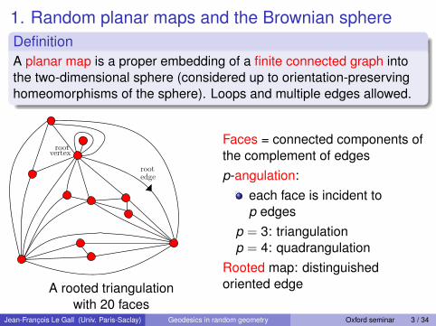
1. Random planar maps and the Brownian sphereDefinitionA planar map is a proper embedding of a finite connected graph intothe two-dimensional sphere (considered up to orientation-preservinghomeomorphisms of the sphere). Loops and multiple edges allowed.
rootedge
rootvertex
A rooted triangulationwith 20 faces
Faces = connected components ofthe complement of edgesp-angulation:
each face is incident top edges
p = 3: triangulationp = 4: quadrangulation
Rooted map: distinguishedoriented edge
Jean-François Le Gall (Univ. Paris-Saclay) Geodesics in random geometry Oxford seminar 3 / 34
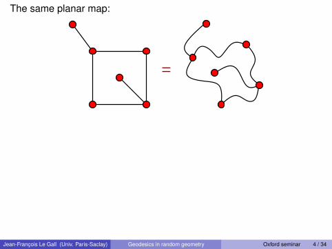
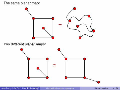
The same planar map:
Two different planar maps:
Jean-François Le Gall (Univ. Paris-Saclay) Geodesics in random geometry Oxford seminar 4 / 34
The same planar map:
Two different planar maps:
Jean-François Le Gall (Univ. Paris-Saclay) Geodesics in random geometry Oxford seminar 4 / 34
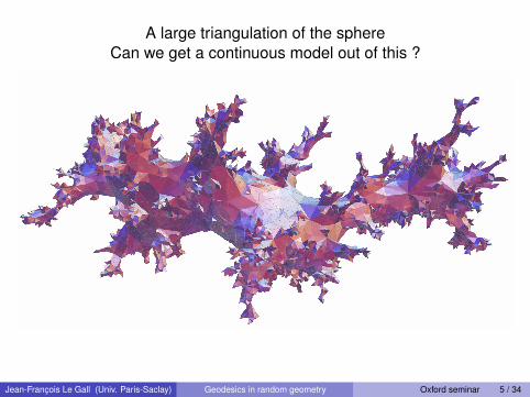
A large triangulation of the sphereCan we get a continuous model out of this ?
Jean-François Le Gall (Univ. Paris-Saclay) Geodesics in random geometry Oxford seminar 5 / 34
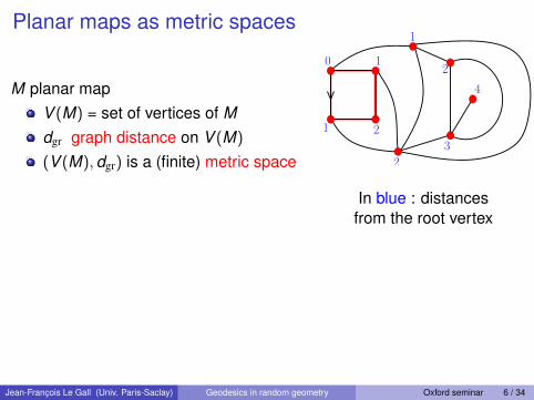
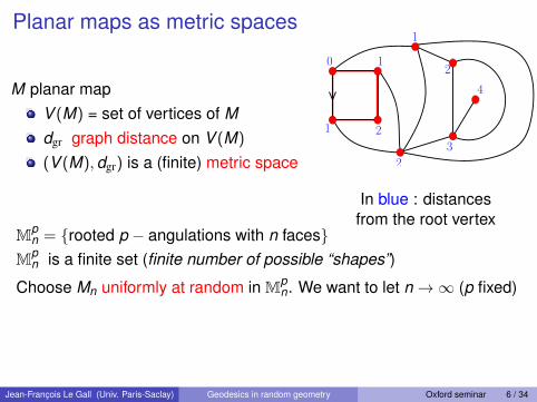
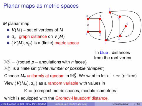
Planar maps as metric spaces
M planar mapV (M) = set of vertices of Mdgr graph distance on V (M)
(V (M),dgr) is a (finite) metric space
0
1
1
2
1
2
2
3
4
In blue : distancesfrom the root vertex
Mpn = {rooted p − angulations with n faces}
Mpn is a finite set (finite number of possible “shapes”)
Choose Mn uniformly at random in Mpn. We want to let n→∞ (p fixed)
View (V (Mn),dgr) as a random variable with values in
K = {compact metric spaces, modulo isometries}which is equipped with the Gromov-Hausdorff distance.
Jean-François Le Gall (Univ. Paris-Saclay) Geodesics in random geometry Oxford seminar 6 / 34
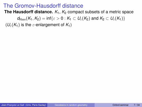
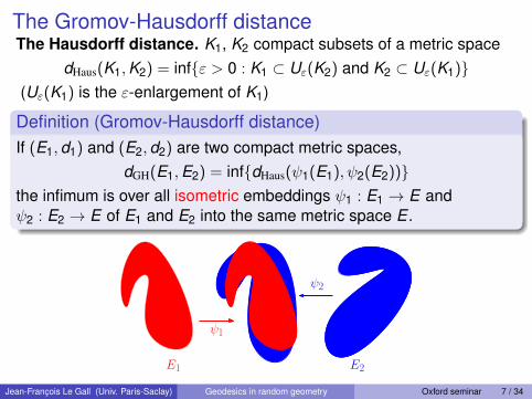
The Gromov-Hausdorff distanceThe Hausdorff distance. K1, K2 compact subsets of a metric space
dHaus(K1,K2) = inf{ε > 0 : K1 ⊂ Uε(K2) and K2 ⊂ Uε(K1)}(Uε(K1) is the ε-enlargement of K1)
Definition (Gromov-Hausdorff distance)If (E1,d1) and (E2,d2) are two compact metric spaces,
dGH(E1,E2) = inf{dHaus(ψ1(E1), ψ2(E2))}the infimum is over all isometric embeddings ψ1 : E1 → E andψ2 : E2 → E of E1 and E2 into the same metric space E .
E1 E2E1
ψ1
ψ2
Jean-François Le Gall (Univ. Paris-Saclay) Geodesics in random geometry Oxford seminar 7 / 34
Gromov-Hausdorff convergence of rescaled maps
FactIf K = {isometry classes of compact metric spaces}, then
(K,dGH) is a separable complete metric space (Polish space)
→ If Mn is uniformly distributed over {p − angulations with n faces},it makes sense to study the convergence in distribution as n→∞ of
(V (Mn),n−adgr)
as random variables with values in K.(Problem stated for triangulations by O. Schramm [ICM, 2006])
Choice of the rescaling factor n−a : a > 0 is chosen so thatdiam(V (Mn)) ≈ na.
⇒ a = 14 [cf Chassaing-Schaeffer PTRF 2004 for quadrangulations]
Jean-François Le Gall (Univ. Paris-Saclay) Geodesics in random geometry Oxford seminar 8 / 34
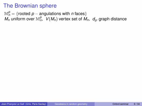
The Brownian sphereMp
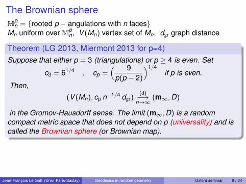
n = {rooted p − angulations with n faces}Mn uniform over Mp
n, V (Mn) vertex set of Mn, dgr graph distance
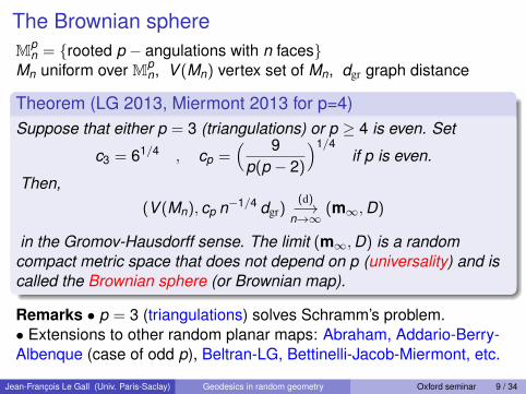
Theorem (LG 2013, Miermont 2013 for p=4)Suppose that either p = 3 (triangulations) or p ≥ 4 is even. Set
c3 = 61/4 , cp =( 9
p(p − 2)
)1/4if p is even.
Then,
(V (Mn), cp n−1/4 dgr)(d)−→
n→∞(m∞,D)
in the Gromov-Hausdorff sense. The limit (m∞,D) is a randomcompact metric space that does not depend on p (universality) and iscalled the Brownian sphere (or Brownian map).
Remarks • p = 3 (triangulations) solves Schramm’s problem.• Extensions to other random planar maps: Abraham, Addario-Berry-Albenque (case of odd p), Beltran-LG, Bettinelli-Jacob-Miermont, etc.
Jean-François Le Gall (Univ. Paris-Saclay) Geodesics in random geometry Oxford seminar 9 / 34
The Brownian sphereMp
n = {rooted p − angulations with n faces}Mn uniform over Mp
n, V (Mn) vertex set of Mn, dgr graph distance
Theorem (LG 2013, Miermont 2013 for p=4)Suppose that either p = 3 (triangulations) or p ≥ 4 is even. Set
c3 = 61/4 , cp =( 9
p(p − 2)
)1/4if p is even.
Then,
(V (Mn), cp n−1/4 dgr)(d)−→
n→∞(m∞,D)
in the Gromov-Hausdorff sense. The limit (m∞,D) is a randomcompact metric space that does not depend on p (universality) and iscalled the Brownian sphere (or Brownian map).
Remarks • p = 3 (triangulations) solves Schramm’s problem.• Extensions to other random planar maps: Abraham, Addario-Berry-Albenque (case of odd p), Beltran-LG, Bettinelli-Jacob-Miermont, etc.
Jean-François Le Gall (Univ. Paris-Saclay) Geodesics in random geometry Oxford seminar 9 / 34
Properties of the Brownian sphere
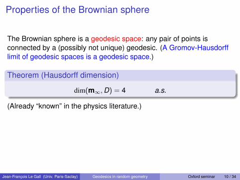
The Brownian sphere is a geodesic space: any pair of points isconnected by a (possibly not unique) geodesic. (A Gromov-Hausdorfflimit of geodesic spaces is a geodesic space.)
Theorem (Hausdorff dimension)
dim(m∞,D) = 4 a.s.
(Already “known” in the physics literature.)
Theorem (topological type)
Almost surely, (m∞,D) is homeomorphic to the 2-sphere S2.
Jean-François Le Gall (Univ. Paris-Saclay) Geodesics in random geometry Oxford seminar 10 / 34
Properties of the Brownian sphere
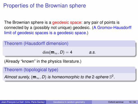
The Brownian sphere is a geodesic space: any pair of points isconnected by a (possibly not unique) geodesic. (A Gromov-Hausdorfflimit of geodesic spaces is a geodesic space.)
Theorem (Hausdorff dimension)
dim(m∞,D) = 4 a.s.
(Already “known” in the physics literature.)
Theorem (topological type)
Almost surely, (m∞,D) is homeomorphic to the 2-sphere S2.
Jean-François Le Gall (Univ. Paris-Saclay) Geodesics in random geometry Oxford seminar 10 / 34
Properties of the Brownian sphere
The Brownian sphere is a geodesic space: any pair of points isconnected by a (possibly not unique) geodesic. (A Gromov-Hausdorfflimit of geodesic spaces is a geodesic space.)
Theorem (Hausdorff dimension)
dim(m∞,D) = 4 a.s.
(Already “known” in the physics literature.)
Theorem (topological type)
Almost surely, (m∞,D) is homeomorphic to the 2-sphere S2.
Jean-François Le Gall (Univ. Paris-Saclay) Geodesics in random geometry Oxford seminar 10 / 34
Connections with Liouville quantum gravity
Miller, Sheffield (2015-2016) have developed a program aiming torelate the Brownian sphere with Liouville quantum gravity:
new construction of the Brownian sphere using the Gaussian freefield and the random growth process called Quantum LoewnerEvolution (an analog of the celebrated SLE processes studied byLawler, Schramm and Werner)this construction makes it possible to equip the Brownian spherewith a conformal structure, and in fact to show that this conformalstructure is determined by the Brownian sphere.
More recently: the Miller-Sheffield construction has been simplified bya direct construction of the Liouville quantum gravity metric from theGaussian free field (Gwynne-Miller 2019 after the work of severalauthors).
Jean-François Le Gall (Univ. Paris-Saclay) Geodesics in random geometry Oxford seminar 11 / 34
2. The construction of the Brownian sphereThe Brownian sphere (m∞,D) is constructed by identifying certainpairs of points in Aldous’ Brownian continuum random tree (CRT).
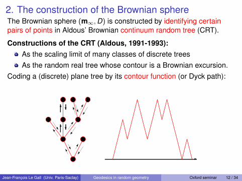
Constructions of the CRT (Aldous, 1991-1993):As the scaling limit of many classes of discrete treesAs the random real tree whose contour is a Brownian excursion.
Coding a (discrete) plane tree by its contour function (or Dyck path):
Jean-François Le Gall (Univ. Paris-Saclay) Geodesics in random geometry Oxford seminar 12 / 34
2. The construction of the Brownian sphereThe Brownian sphere (m∞,D) is constructed by identifying certainpairs of points in Aldous’ Brownian continuum random tree (CRT).
Constructions of the CRT (Aldous, 1991-1993):As the scaling limit of many classes of discrete treesAs the random real tree whose contour is a Brownian excursion.
Coding a (discrete) plane tree by its contour function (or Dyck path):
Jean-François Le Gall (Univ. Paris-Saclay) Geodesics in random geometry Oxford seminar 12 / 34
The notion of a real tree
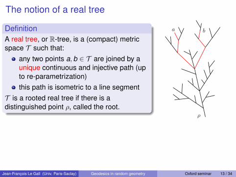
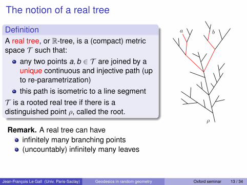
DefinitionA real tree, or R-tree, is a (compact) metricspace T such that:
any two points a,b ∈ T are joined by aunique continuous and injective path (upto re-parametrization)this path is isometric to a line segment
T is a rooted real tree if there is adistinguished point ρ, called the root.
ρ
a b
Remark. A real tree can haveinfinitely many branching points(uncountably) infinitely many leaves
Fact. The coding of discrete trees by contour functions can beextended to real trees: also gives a cyclic ordering on the tree.
Jean-François Le Gall (Univ. Paris-Saclay) Geodesics in random geometry Oxford seminar 13 / 34
The notion of a real tree
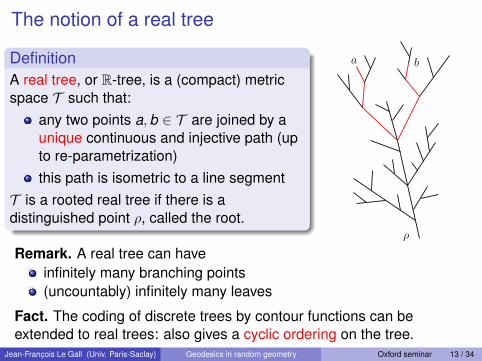
DefinitionA real tree, or R-tree, is a (compact) metricspace T such that:
any two points a,b ∈ T are joined by aunique continuous and injective path (upto re-parametrization)this path is isometric to a line segment
T is a rooted real tree if there is adistinguished point ρ, called the root.
ρ
a b
Remark. A real tree can haveinfinitely many branching points(uncountably) infinitely many leaves
Fact. The coding of discrete trees by contour functions can beextended to real trees: also gives a cyclic ordering on the tree.
Jean-François Le Gall (Univ. Paris-Saclay) Geodesics in random geometry Oxford seminar 13 / 34
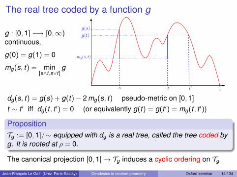
The real tree coded by a function g
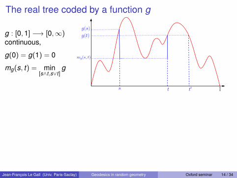
g : [0,1] −→ [0,∞)continuous,
g(0) = g(1) = 0
mg(s, t) = min[s∧t ,s∨t]
g
s t t′
mg(s, t)
g(t)
g(s)
1
dg(s, t) = g(s) + g(t)− 2 mg(s, t) pseudo-metric on [0,1]
t ∼ t ′ iff dg(t , t ′) = 0 (or equivalently g(t) = g(t ′) = mg(t , t ′))
PropositionTg := [0,1]/∼ equipped with dg is a real tree, called the tree coded byg. It is rooted at ρ = 0.
The canonical projection [0,1]→ Tg induces a cyclic ordering on Tg
Jean-François Le Gall (Univ. Paris-Saclay) Geodesics in random geometry Oxford seminar 14 / 34
The real tree coded by a function g
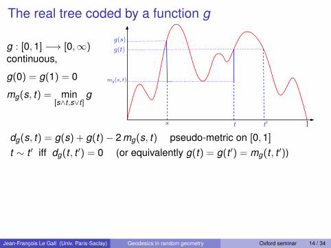
g : [0,1] −→ [0,∞)continuous,
g(0) = g(1) = 0
mg(s, t) = min[s∧t ,s∨t]
g
s t t′
mg(s, t)
g(t)
g(s)
1
dg(s, t) = g(s) + g(t)− 2 mg(s, t) pseudo-metric on [0,1]
t ∼ t ′ iff dg(t , t ′) = 0 (or equivalently g(t) = g(t ′) = mg(t , t ′))
PropositionTg := [0,1]/∼ equipped with dg is a real tree, called the tree coded byg. It is rooted at ρ = 0.
The canonical projection [0,1]→ Tg induces a cyclic ordering on Tg
Jean-François Le Gall (Univ. Paris-Saclay) Geodesics in random geometry Oxford seminar 14 / 34
The real tree coded by a function g
g : [0,1] −→ [0,∞)continuous,
g(0) = g(1) = 0
mg(s, t) = min[s∧t ,s∨t]
g
s t t′
mg(s, t)
g(t)
g(s)
1
dg(s, t) = g(s) + g(t)− 2 mg(s, t) pseudo-metric on [0,1]
t ∼ t ′ iff dg(t , t ′) = 0 (or equivalently g(t) = g(t ′) = mg(t , t ′))
PropositionTg := [0,1]/∼ equipped with dg is a real tree, called the tree coded byg. It is rooted at ρ = 0.
The canonical projection [0,1]→ Tg induces a cyclic ordering on Tg
Jean-François Le Gall (Univ. Paris-Saclay) Geodesics in random geometry Oxford seminar 14 / 34
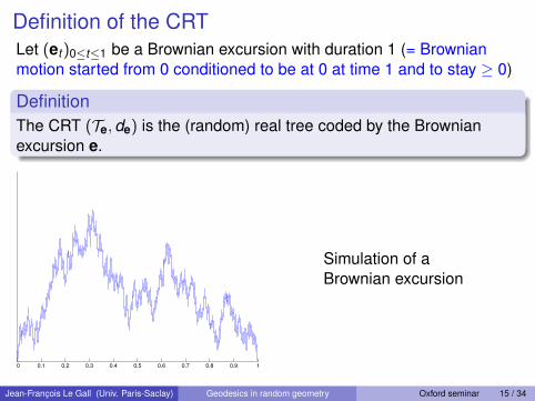
Definition of the CRTLet (et )0≤t≤1 be a Brownian excursion with duration 1 (= Brownianmotion started from 0 conditioned to be at 0 at time 1 and to stay ≥ 0)
DefinitionThe CRT (Te,de) is the (random) real tree coded by the Brownianexcursion e.
0 0.1 0.2 0.3 0.4 0.5 0.6 0.7 0.8 0.9 1
Simulation of aBrownian excursion
Jean-François Le Gall (Univ. Paris-Saclay) Geodesics in random geometry Oxford seminar 15 / 34
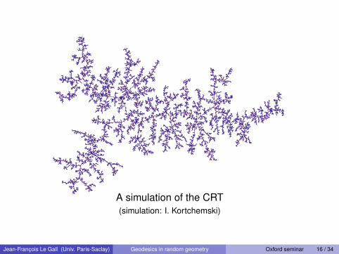
A simulation of the CRT(simulation: I. Kortchemski)
Jean-François Le Gall (Univ. Paris-Saclay) Geodesics in random geometry Oxford seminar 16 / 34
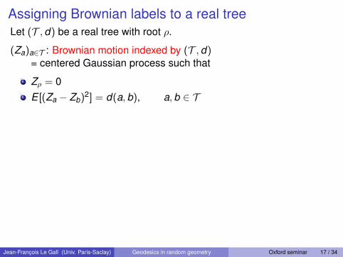
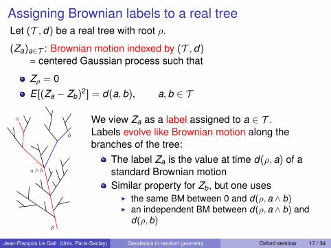
Assigning Brownian labels to a real treeLet (T ,d) be a real tree with root ρ.
(Za)a∈T : Brownian motion indexed by (T ,d)= centered Gaussian process such that
Zρ = 0E [(Za − Zb)2] = d(a,b), a,b ∈ T
ρ
a
b
a ∧ b
We view Za as a label assigned to a ∈ T .Labels evolve like Brownian motion along thebranches of the tree:
The label Za is the value at time d(ρ,a) of astandard Brownian motionSimilar property for Zb, but one uses
I the same BM between 0 and d(ρ,a ∧ b)I an independent BM between d(ρ,a ∧ b) and
d(ρ,b)
Jean-François Le Gall (Univ. Paris-Saclay) Geodesics in random geometry Oxford seminar 17 / 34
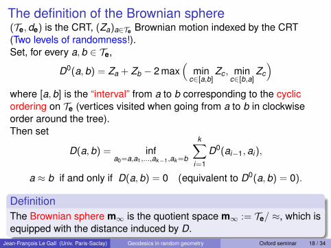
The definition of the Brownian sphere(Te,de) is the CRT, (Za)a∈Te Brownian motion indexed by the CRT(Two levels of randomness!).
Set, for every a,b ∈ Te,
D0(a,b) = Za + Zb − 2 max(
minc∈[a,b]
Zc , minc∈[b,a]
Zc
)where [a,b] is the “interval” from a to b corresponding to the cyclicordering on Te (vertices visited when going from a to b in clockwiseorder around the tree).Then set
D(a,b) = infa0=a,a1,...,ak−1,ak=b
k∑i=1
D0(ai−1,ai),
a ≈ b if and only if D(a,b) = 0 (equivalent to D0(a,b) = 0).
DefinitionThe Brownian sphere m∞ is the quotient space m∞ := Te/ ≈, which isequipped with the distance induced by D.
Jean-François Le Gall (Univ. Paris-Saclay) Geodesics in random geometry Oxford seminar 18 / 34
The definition of the Brownian sphere(Te,de) is the CRT, (Za)a∈Te Brownian motion indexed by the CRT(Two levels of randomness!).Set, for every a,b ∈ Te,
D0(a,b) = Za + Zb − 2 max(
minc∈[a,b]
Zc , minc∈[b,a]
Zc
)where [a,b] is the “interval” from a to b corresponding to the cyclicordering on Te (vertices visited when going from a to b in clockwiseorder around the tree).
Then set
D(a,b) = infa0=a,a1,...,ak−1,ak=b
k∑i=1
D0(ai−1,ai),
a ≈ b if and only if D(a,b) = 0 (equivalent to D0(a,b) = 0).
DefinitionThe Brownian sphere m∞ is the quotient space m∞ := Te/ ≈, which isequipped with the distance induced by D.
Jean-François Le Gall (Univ. Paris-Saclay) Geodesics in random geometry Oxford seminar 18 / 34
The definition of the Brownian sphere(Te,de) is the CRT, (Za)a∈Te Brownian motion indexed by the CRT(Two levels of randomness!).Set, for every a,b ∈ Te,
D0(a,b) = Za + Zb − 2 max(
minc∈[a,b]
Zc , minc∈[b,a]
Zc
)where [a,b] is the “interval” from a to b corresponding to the cyclicordering on Te (vertices visited when going from a to b in clockwiseorder around the tree).Then set
D(a,b) = infa0=a,a1,...,ak−1,ak=b
k∑i=1
D0(ai−1,ai),
a ≈ b if and only if D(a,b) = 0 (equivalent to D0(a,b) = 0).
DefinitionThe Brownian sphere m∞ is the quotient space m∞ := Te/ ≈, which isequipped with the distance induced by D.
Jean-François Le Gall (Univ. Paris-Saclay) Geodesics in random geometry Oxford seminar 18 / 34
The definition of the Brownian sphere(Te,de) is the CRT, (Za)a∈Te Brownian motion indexed by the CRT(Two levels of randomness!).Set, for every a,b ∈ Te,
D0(a,b) = Za + Zb − 2 max(
minc∈[a,b]
Zc , minc∈[b,a]
Zc
)where [a,b] is the “interval” from a to b corresponding to the cyclicordering on Te (vertices visited when going from a to b in clockwiseorder around the tree).Then set
D(a,b) = infa0=a,a1,...,ak−1,ak=b
k∑i=1
D0(ai−1,ai),
a ≈ b if and only if D(a,b) = 0 (equivalent to D0(a,b) = 0).
DefinitionThe Brownian sphere m∞ is the quotient space m∞ := Te/ ≈, which isequipped with the distance induced by D.
Jean-François Le Gall (Univ. Paris-Saclay) Geodesics in random geometry Oxford seminar 18 / 34
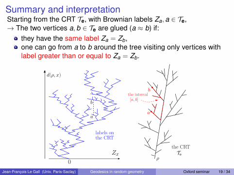
Summary and interpretationStarting from the CRT Te, with Brownian labels Za,a ∈ Te,→ The two vertices a,b ∈ Te are glued (a ≈ b) if:
they have the same label Za = Zb,one can go from a to b around the tree visiting only vertices withlabel greater than or equal to Za = Zb.
a
b
a
bthe interval[a, b]
d(ρ, x)
ρZx
0
the CRTTe
labels onthe CRT
Jean-François Le Gall (Univ. Paris-Saclay) Geodesics in random geometry Oxford seminar 19 / 34
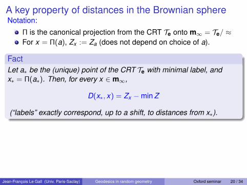
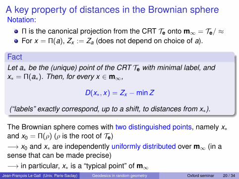
A key property of distances in the Brownian sphereNotation:
Π is the canonical projection from the CRT Te onto m∞ = Te/ ≈For x = Π(a), Zx := Za (does not depend on choice of a).
FactLet a∗ be the (unique) point of the CRT Te with minimal label, andx∗ = Π(a∗). Then, for every x ∈ m∞,
D(x∗, x) = Zx −min Z
(“labels” exactly correspond, up to a shift, to distances from x∗).
The Brownian sphere comes with two distinguished points, namely x∗and x0 = Π(ρ) (ρ is the root of Te)−→ x0 and x∗ are independently uniformly distributed over m∞ (in asense that can be made precise)−→ in particular, x∗ is a “typical point” of m∞
Jean-François Le Gall (Univ. Paris-Saclay) Geodesics in random geometry Oxford seminar 20 / 34
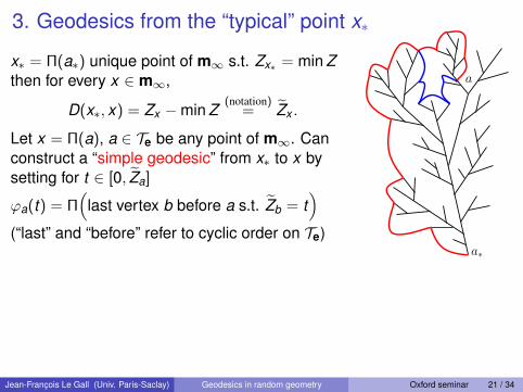
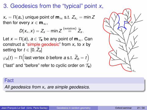
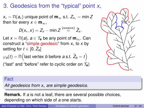
3. Geodesics from the “typical” point x∗
x∗ = Π(a∗) unique point of m∞ s.t. Zx∗ = min Zthen for every x ∈ m∞,
D(x∗, x) = Zx −min Z(notation)
= Z̃x .
Let x = Π(a), a ∈ Te be any point of m∞. Canconstruct a “simple geodesic” from x∗ to x bysetting for t ∈ [0, Z̃a]
ϕa(t) = Π(
last vertex b before a s.t. Z̃b = t)
(“last” and “before” refer to cyclic order on Te)
a
a∗
FactAll geodesics from x∗ are simple geodesics.
Remark. If a is not a leaf, there are several possible choices,depending on which side of a one starts.
Jean-François Le Gall (Univ. Paris-Saclay) Geodesics in random geometry Oxford seminar 21 / 34
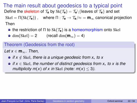
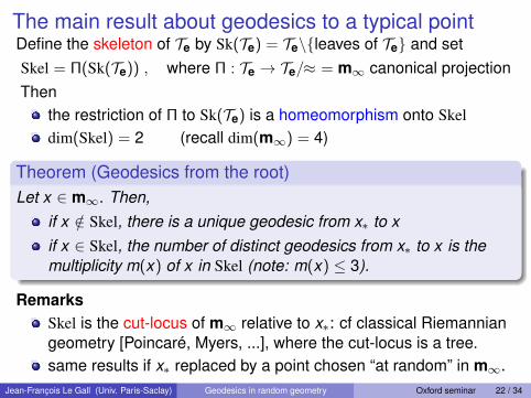
The main result about geodesics to a typical pointDefine the skeleton of Te by Sk(Te) = Te\{leaves of Te} and setSkel = Π(Sk(Te)) , where Π : Te → Te/≈ = m∞ canonical projectionThen
the restriction of Π to Sk(Te) is a homeomorphism onto Skeldim(Skel) = 2 (recall dim(m∞) = 4)
Theorem (Geodesics from the root)Let x ∈ m∞. Then,
if x /∈ Skel, there is a unique geodesic from x∗ to xif x ∈ Skel, the number of distinct geodesics from x∗ to x is themultiplicity m(x) of x in Skel (note: m(x) ≤ 3).
RemarksSkel is the cut-locus of m∞ relative to x∗: cf classical Riemanniangeometry [Poincaré, Myers, ...], where the cut-locus is a tree.same results if x∗ replaced by a point chosen “at random” in m∞.
Jean-François Le Gall (Univ. Paris-Saclay) Geodesics in random geometry Oxford seminar 22 / 34
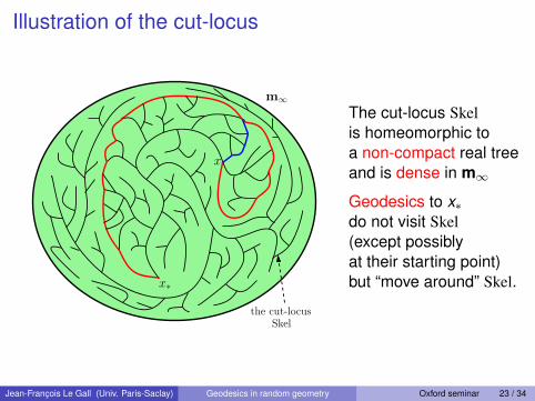
Illustration of the cut-locus
x
m∞
the cut-locusSkel
x∗
The cut-locus Skelis homeomorphic toa non-compact real treeand is dense in m∞
Geodesics to x∗do not visit Skel(except possiblyat their starting point)but “move around” Skel.
Jean-François Le Gall (Univ. Paris-Saclay) Geodesics in random geometry Oxford seminar 23 / 34
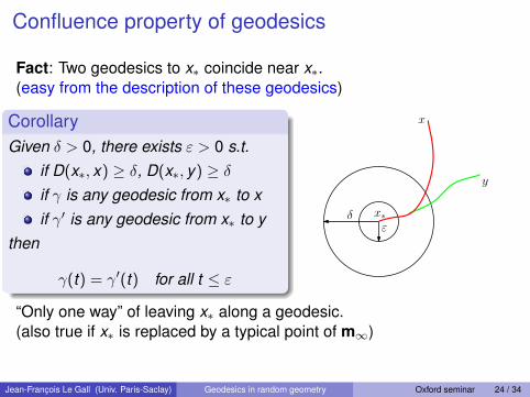
Confluence property of geodesics
Fact: Two geodesics to x∗ coincide near x∗.(easy from the description of these geodesics)
CorollaryGiven δ > 0, there exists ε > 0 s.t.
if D(x∗, x) ≥ δ, D(x∗, y) ≥ δif γ is any geodesic from x∗ to xif γ′ is any geodesic from x∗ to y
then
γ(t) = γ′(t) for all t ≤ ε
εδ
x
y
x∗
“Only one way” of leaving x∗ along a geodesic.(also true if x∗ is replaced by a typical point of m∞)
Jean-François Le Gall (Univ. Paris-Saclay) Geodesics in random geometry Oxford seminar 24 / 34
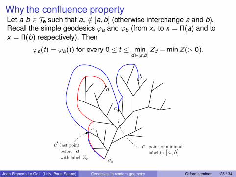
Why the confluence propertyLet a,b ∈ Te such that a∗ /∈ [a,b] (otherwise interchange a and b).Recall the simple geodesics ϕa and ϕb (from x∗ to x = Π(a) and tox = Π(b) respectively). Then
ϕa(t) = ϕb(t) for every 0 ≤ t ≤ mind∈[a,b]
Zd −min Z (> 0).
a
b
a∗
c
c point of minimal
label in [a, b]
c′
c′ last pointbefore awith label Zc
Jean-François Le Gall (Univ. Paris-Saclay) Geodesics in random geometry Oxford seminar 25 / 34
4. Geodesics between exceptional points
If x and y are typical points of the Brownian sphere (chosen accordingto the volume measure)
There is a unique geodesic from y to x (can take x = x∗, thecut-locus has zero volume)
If x is typical (say x = x∗) then for “exceptional points” y :
There can be up to 3 geodesics from y to x .
If x and y are both exceptional:
There can be up to 9 geodesics from y to x ( Miller-Qian (2020),following earlier work of Angel, Kolesnik, Miermont (2017)).Miller-Qian (2020) even compute the Hausdorff dimension of theset of pairs (x , y) such that there are exactly k geodesics from yto x .
Jean-François Le Gall (Univ. Paris-Saclay) Geodesics in random geometry Oxford seminar 26 / 34
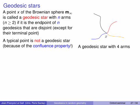
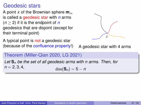
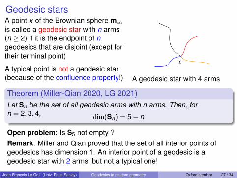
Geodesic starsA point x of the Brownian sphere m∞is called a geodesic star with n arms(n ≥ 2) if it is the endpoint of ngeodesics that are disjoint (except fortheir terminal point)
A typical point is not a geodesic star(because of the confluence property!)
x
A geodesic star with 4 arms
Theorem (Miller-Qian 2020, LG 2021)Let Sn be the set of all geodesic arms with n arms. Then, forn = 2,3,4, dim(Sn) = 5− n
Open problem: Is S5 not empty ?Remark. Miller and Qian proved that the set of all interior points ofgeodesics has dimension 1. An interior point of a geodesic is ageodesic star with 2 arms, but not a typical one!
Jean-François Le Gall (Univ. Paris-Saclay) Geodesics in random geometry Oxford seminar 27 / 34
Results on geodesics in the Brownian sphere
Miermont 2009 (Ann. ENS): uniqueness of the geodesic betweentwo typical points (also in higher genus)
LG 2010 (Acta Math.): complete description of geodesics from atypical pointMiermont 2013 (Acta Math.): uses the notion of geodesic stars toprove uniqueness of the Brownian sphereAngel, Kolesnik, Miermont 2017 (Ann. Probab.) First results aboutgeodesic networks (union of the geodesics connecting two points)Miller, Qian 2020 Full description of geodesic networks. Upperbound on the dimension of geodesic starsLG 2021 Lower bound matching the upper bound of Miller-Qianfor geodesic stars.Related results in Liouville quantum gravity: Gwynne-Miller (2019)on the confluence property, Gwynne (2020) on geodesic networks.
Jean-François Le Gall (Univ. Paris-Saclay) Geodesics in random geometry Oxford seminar 28 / 34
Results on geodesics in the Brownian sphere
Miermont 2009 (Ann. ENS): uniqueness of the geodesic betweentwo typical points (also in higher genus)LG 2010 (Acta Math.): complete description of geodesics from atypical point
Miermont 2013 (Acta Math.): uses the notion of geodesic stars toprove uniqueness of the Brownian sphereAngel, Kolesnik, Miermont 2017 (Ann. Probab.) First results aboutgeodesic networks (union of the geodesics connecting two points)Miller, Qian 2020 Full description of geodesic networks. Upperbound on the dimension of geodesic starsLG 2021 Lower bound matching the upper bound of Miller-Qianfor geodesic stars.Related results in Liouville quantum gravity: Gwynne-Miller (2019)on the confluence property, Gwynne (2020) on geodesic networks.
Jean-François Le Gall (Univ. Paris-Saclay) Geodesics in random geometry Oxford seminar 28 / 34
Results on geodesics in the Brownian sphere
Miermont 2009 (Ann. ENS): uniqueness of the geodesic betweentwo typical points (also in higher genus)LG 2010 (Acta Math.): complete description of geodesics from atypical pointMiermont 2013 (Acta Math.): uses the notion of geodesic stars toprove uniqueness of the Brownian sphere
Angel, Kolesnik, Miermont 2017 (Ann. Probab.) First results aboutgeodesic networks (union of the geodesics connecting two points)Miller, Qian 2020 Full description of geodesic networks. Upperbound on the dimension of geodesic starsLG 2021 Lower bound matching the upper bound of Miller-Qianfor geodesic stars.Related results in Liouville quantum gravity: Gwynne-Miller (2019)on the confluence property, Gwynne (2020) on geodesic networks.
Jean-François Le Gall (Univ. Paris-Saclay) Geodesics in random geometry Oxford seminar 28 / 34
Results on geodesics in the Brownian sphere
Miermont 2009 (Ann. ENS): uniqueness of the geodesic betweentwo typical points (also in higher genus)LG 2010 (Acta Math.): complete description of geodesics from atypical pointMiermont 2013 (Acta Math.): uses the notion of geodesic stars toprove uniqueness of the Brownian sphereAngel, Kolesnik, Miermont 2017 (Ann. Probab.) First results aboutgeodesic networks (union of the geodesics connecting two points)
Miller, Qian 2020 Full description of geodesic networks. Upperbound on the dimension of geodesic starsLG 2021 Lower bound matching the upper bound of Miller-Qianfor geodesic stars.Related results in Liouville quantum gravity: Gwynne-Miller (2019)on the confluence property, Gwynne (2020) on geodesic networks.
Jean-François Le Gall (Univ. Paris-Saclay) Geodesics in random geometry Oxford seminar 28 / 34
Results on geodesics in the Brownian sphere
Miermont 2009 (Ann. ENS): uniqueness of the geodesic betweentwo typical points (also in higher genus)LG 2010 (Acta Math.): complete description of geodesics from atypical pointMiermont 2013 (Acta Math.): uses the notion of geodesic stars toprove uniqueness of the Brownian sphereAngel, Kolesnik, Miermont 2017 (Ann. Probab.) First results aboutgeodesic networks (union of the geodesics connecting two points)Miller, Qian 2020 Full description of geodesic networks. Upperbound on the dimension of geodesic stars
LG 2021 Lower bound matching the upper bound of Miller-Qianfor geodesic stars.Related results in Liouville quantum gravity: Gwynne-Miller (2019)on the confluence property, Gwynne (2020) on geodesic networks.
Jean-François Le Gall (Univ. Paris-Saclay) Geodesics in random geometry Oxford seminar 28 / 34
Results on geodesics in the Brownian sphere
Miermont 2009 (Ann. ENS): uniqueness of the geodesic betweentwo typical points (also in higher genus)LG 2010 (Acta Math.): complete description of geodesics from atypical pointMiermont 2013 (Acta Math.): uses the notion of geodesic stars toprove uniqueness of the Brownian sphereAngel, Kolesnik, Miermont 2017 (Ann. Probab.) First results aboutgeodesic networks (union of the geodesics connecting two points)Miller, Qian 2020 Full description of geodesic networks. Upperbound on the dimension of geodesic starsLG 2021 Lower bound matching the upper bound of Miller-Qianfor geodesic stars.
Related results in Liouville quantum gravity: Gwynne-Miller (2019)on the confluence property, Gwynne (2020) on geodesic networks.
Jean-François Le Gall (Univ. Paris-Saclay) Geodesics in random geometry Oxford seminar 28 / 34
Results on geodesics in the Brownian sphere
Miermont 2009 (Ann. ENS): uniqueness of the geodesic betweentwo typical points (also in higher genus)LG 2010 (Acta Math.): complete description of geodesics from atypical pointMiermont 2013 (Acta Math.): uses the notion of geodesic stars toprove uniqueness of the Brownian sphereAngel, Kolesnik, Miermont 2017 (Ann. Probab.) First results aboutgeodesic networks (union of the geodesics connecting two points)Miller, Qian 2020 Full description of geodesic networks. Upperbound on the dimension of geodesic starsLG 2021 Lower bound matching the upper bound of Miller-Qianfor geodesic stars.Related results in Liouville quantum gravity: Gwynne-Miller (2019)on the confluence property, Gwynne (2020) on geodesic networks.
Jean-François Le Gall (Univ. Paris-Saclay) Geodesics in random geometry Oxford seminar 28 / 34
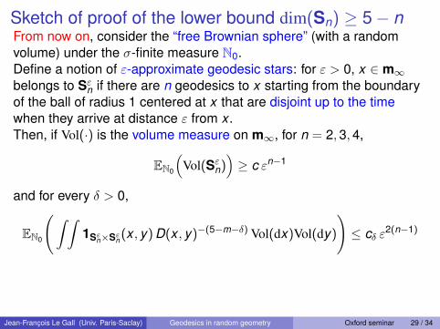
Sketch of proof of the lower bound dim(Sn) ≥ 5− nFrom now on, consider the “free Brownian sphere” (with a randomvolume) under the σ-finite measure N0.Define a notion of ε-approximate geodesic stars: for ε > 0, x ∈ m∞belongs to Sεn if there are n geodesics to x starting from the boundaryof the ball of radius 1 centered at x that are disjoint up to the timewhen they arrive at distance ε from x .
Then, if Vol(·) is the volume measure on m∞, for n = 2,3,4,
EN0
(Vol(Sεn)
)≥ c εn−1
and for every δ > 0,
EN0
(∫ ∫1Sε
n×Sεn(x , y) D(x , y)−(5−m−δ) Vol(dx)Vol(dy)
)≤ cδ ε2(n−1)
−→ Standard techniques (extraction of convergent subsequence fromε−(n−1)Vol|Sε
n, Frostman lemma) then show that Sn =
⋂ε>0 Sεn has
dimension ≥ 5− n on an event of positive N0-measure.
Jean-François Le Gall (Univ. Paris-Saclay) Geodesics in random geometry Oxford seminar 29 / 34
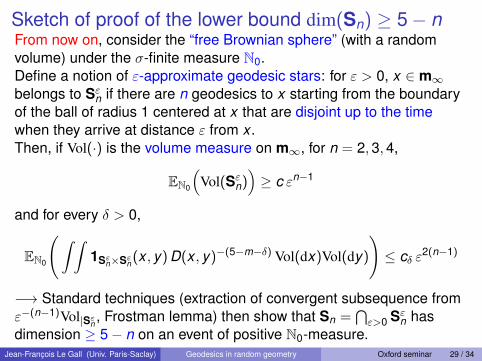
Sketch of proof of the lower bound dim(Sn) ≥ 5− nFrom now on, consider the “free Brownian sphere” (with a randomvolume) under the σ-finite measure N0.Define a notion of ε-approximate geodesic stars: for ε > 0, x ∈ m∞belongs to Sεn if there are n geodesics to x starting from the boundaryof the ball of radius 1 centered at x that are disjoint up to the timewhen they arrive at distance ε from x .Then, if Vol(·) is the volume measure on m∞, for n = 2,3,4,
EN0
(Vol(Sεn)
)≥ c εn−1
and for every δ > 0,
EN0
(∫ ∫1Sε
n×Sεn(x , y) D(x , y)−(5−m−δ) Vol(dx)Vol(dy)
)≤ cδ ε2(n−1)
−→ Standard techniques (extraction of convergent subsequence fromε−(n−1)Vol|Sε
n, Frostman lemma) then show that Sn =
⋂ε>0 Sεn has
dimension ≥ 5− n on an event of positive N0-measure.
Jean-François Le Gall (Univ. Paris-Saclay) Geodesics in random geometry Oxford seminar 29 / 34
Sketch of proof of the lower bound dim(Sn) ≥ 5− nFrom now on, consider the “free Brownian sphere” (with a randomvolume) under the σ-finite measure N0.Define a notion of ε-approximate geodesic stars: for ε > 0, x ∈ m∞belongs to Sεn if there are n geodesics to x starting from the boundaryof the ball of radius 1 centered at x that are disjoint up to the timewhen they arrive at distance ε from x .Then, if Vol(·) is the volume measure on m∞, for n = 2,3,4,
EN0
(Vol(Sεn)
)≥ c εn−1
and for every δ > 0,
EN0
(∫ ∫1Sε
n×Sεn(x , y) D(x , y)−(5−m−δ) Vol(dx)Vol(dy)
)≤ cδ ε2(n−1)
−→ Standard techniques (extraction of convergent subsequence fromε−(n−1)Vol|Sε
n, Frostman lemma) then show that Sn =
⋂ε>0 Sεn has
dimension ≥ 5− n on an event of positive N0-measure.Jean-François Le Gall (Univ. Paris-Saclay) Geodesics in random geometry Oxford seminar 29 / 34
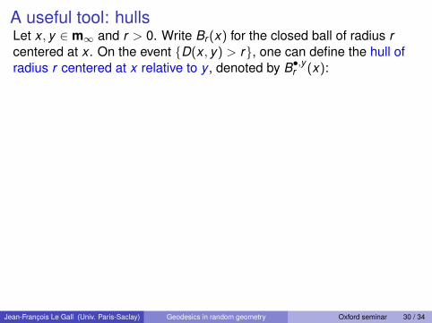
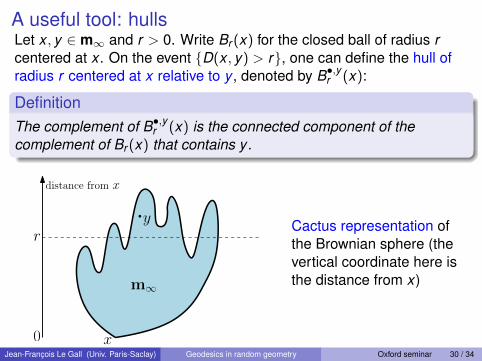
A useful tool: hullsLet x , y ∈ m∞ and r > 0. Write Br (x) for the closed ball of radius rcentered at x . On the event {D(x , y) > r}, one can define the hull ofradius r centered at x relative to y , denoted by B•,yr (x):
DefinitionThe complement of B•,yr (x) is the connected component of thecomplement of Br (x) that contains y.
x
y
0
r
m∞
distance from x
Cactus representation ofthe Brownian sphere (thevertical coordinate here isthe distance from x)
Jean-François Le Gall (Univ. Paris-Saclay) Geodesics in random geometry Oxford seminar 30 / 34
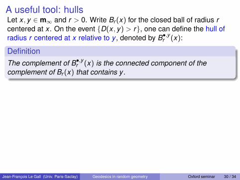
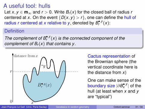
A useful tool: hullsLet x , y ∈ m∞ and r > 0. Write Br (x) for the closed ball of radius rcentered at x . On the event {D(x , y) > r}, one can define the hull ofradius r centered at x relative to y , denoted by B•,yr (x):
DefinitionThe complement of B•,yr (x) is the connected component of thecomplement of Br (x) that contains y.
x
y
0
ry
distance fromx
B•,yr (x)
Cactus representation ofthe Brownian sphere (thevertical coordinate here isthe distance from x)
One can make sense of theboundary size |∂B•,yx | of thehull (at least when x and yare “typical”)
Jean-François Le Gall (Univ. Paris-Saclay) Geodesics in random geometry Oxford seminar 31 / 34
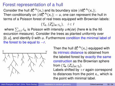
Forest representation of a hullConsider the hull B•,x0
r (x∗) and its boundary size |∂B•,x0r (x∗)|.
Then conditionally on |∂B•,x0r (x∗)| = u, one can represent the hull in
terms of a Poisson forest of real trees equipped with Brownian labels:(Tei , (Z
ia)a∈Tei
), i ∈ Iwhere
∑i∈I δei is Poisson with intensity u n(de) (here n is the Itô
excursion measure). Consider the trees as planted uniformly over[0,u], and identify 0 with u. Furthermore condition the minimal label ofthe forest to be equal to −r .
0 uThen the hull B•,x0
r (x∗) equipped withits intrinsic distance is obtained fromthe labeled forest by exactly the sameconstruction as the Brownian spherefrom (Te, (Za)a∈Te).Labels shifted by +r again correspondto distances from the point x∗, which isthe point with minimal label.
Jean-François Le Gall (Univ. Paris-Saclay) Geodesics in random geometry Oxford seminar 32 / 34
The one-point estimate
0 u
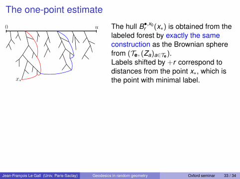
x∗
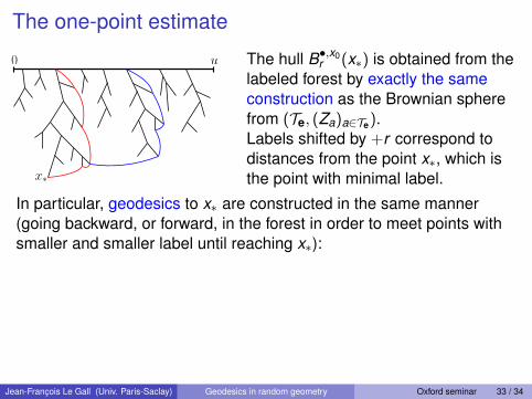
The hull B•,x0r (x∗) is obtained from the
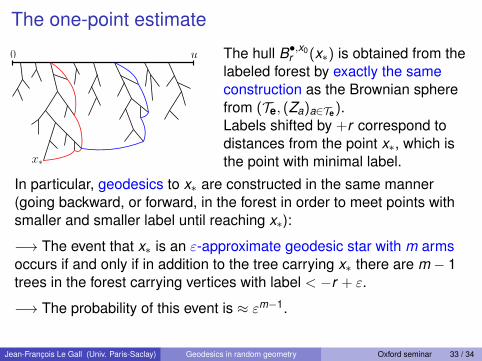
labeled forest by exactly the sameconstruction as the Brownian spherefrom (Te, (Za)a∈Te).Labels shifted by +r correspond todistances from the point x∗, which isthe point with minimal label.
In particular, geodesics to x∗ are constructed in the same manner(going backward, or forward, in the forest in order to meet points withsmaller and smaller label until reaching x∗):
−→ The event that x∗ is an ε-approximate geodesic star with m armsoccurs if and only if in addition to the tree carrying x∗ there are m − 1trees in the forest carrying vertices with label < −r + ε.
−→ The probability of this event is ≈ εm−1.
Jean-François Le Gall (Univ. Paris-Saclay) Geodesics in random geometry Oxford seminar 33 / 34
The one-point estimate
0 u
x∗
The hull B•,x0r (x∗) is obtained from the
labeled forest by exactly the sameconstruction as the Brownian spherefrom (Te, (Za)a∈Te).Labels shifted by +r correspond todistances from the point x∗, which isthe point with minimal label.
In particular, geodesics to x∗ are constructed in the same manner(going backward, or forward, in the forest in order to meet points withsmaller and smaller label until reaching x∗):
−→ The event that x∗ is an ε-approximate geodesic star with m armsoccurs if and only if in addition to the tree carrying x∗ there are m − 1trees in the forest carrying vertices with label < −r + ε.
−→ The probability of this event is ≈ εm−1.
Jean-François Le Gall (Univ. Paris-Saclay) Geodesics in random geometry Oxford seminar 33 / 34
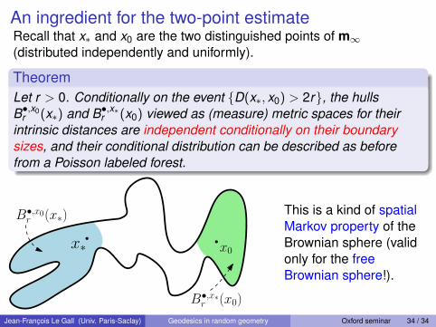
An ingredient for the two-point estimateRecall that x∗ and x0 are the two distinguished points of m∞(distributed independently and uniformly).
TheoremLet r > 0. Conditionally on the event {D(x∗, x0) > 2r}, the hullsB•,x0
r (x∗) and B•,x∗r (x0) viewed as (measure) metric spaces for theirintrinsic distances are independent conditionally on their boundarysizes, and their conditional distribution can be described as beforefrom a Poisson labeled forest.
x0x∗
B•,x0r (x∗)
B•,x∗r (x0)
This is a kind of spatialMarkov property of theBrownian sphere (validonly for the freeBrownian sphere!).
Jean-François Le Gall (Univ. Paris-Saclay) Geodesics in random geometry Oxford seminar 34 / 34