climatic variability and irrigation: an analysis of...
TRANSCRIPT
1
Climatic Variability and Irrigation: An Analysis of Irrigation Efficiency
Patterns in U.S. Counties
Eric Njuki
University of Connecticut
Boris E. Bravo-Ureta
University of Connecticut
Selected Paper prepared for presentation at the 2016 Agricultural & Applied Economics
Association Annual Meeting, Boston, Massachusetts, July 31-August 2
2
The efficient management of water resources, given rising water demand and projected
reductions in precipitation as a direct result of climate change, has become a critical issue.
Several regions in the U.S. continue to experience significant drought and water shortages, which
directly threatens the viability of agriculture. This has led to an increase in irrigation, which is in
direct competition with other uses of water for domestic, industrial, and hydroelectric activities.
Consequently, conservation and efficient water use has emerged as an important focal point in
water policy related issues in the U.S. (Clemmens et al. 2008; USDA 2014).
The evidence within the United States that establishes the connection between climatic
variability and the need for secondary sources of water, such as irrigation, has been building for
years. A major argument has been that changing temperature and precipitation patterns will lead
directly to modifications in farming systems and resource use (e.g., Mendelsohn, Nordhaus and
Shaw 1994; Adams et al. 1995; Mendelsohn and Dinar 2003; Deschenes and Greenstone 2007;
Schlenker and Roberts 2009; Hatfield et al. 2014). Most importantly, some of these studies have
noted a growing reliance on irrigation (e.g., Mendelsohn and Dinar 2003; Schlenker, Hanneman
and Fisher 2005; Deschenes and Greenstone 2007; Hatfield et al. 2014). The implementation of
such adaptation strategies can be expected, on the one hand, to reduce the long-run adverse
effects stemming from changes in climatic conditions (Schlenker, Hanemann and Fisher 2005),
while on the other, putting further pressure on a resource that is becoming increasingly scarce.
These developments are clearly not compatible and are likely to increase tensions between
farmers and other sectors of the economy (Schaible and Aillery 2012).
According to the U.S. Geological Survey (USGS), the agricultural sector is the second
largest consumer of water resources in United States. Combined water withdrawals used in
irrigation, livestock and aquaculture accounted for approximately 115,000 million gallons per
3
day, with 62.4 million acres of land under irrigation (USGS 2014). Moreover, U.S. farmers are
shifting to higher revenue crops while several climate models predict significant changes in
weather, characterized by warmer temperatures and lower precipitation. As a result, it is
expected that demand for water will continue to surpass its supply resulting in a strain in water
available for household and industrial purposes (Schaible and Aillery 2014). Hence, the threat of
water scarcity has become an issue of concern among policy makers and stakeholders alike with
conversations on how best to manage this scarce resource being brought to the forefront (e.g.,
McGuckin, Gollehon, and Ghosh 1992; Weinberg, Kling, and Wilen 1993; Chakraborty, Misra,
and Johnson 2002; Wu, Devadoss, and Lu 2003; Lilienfeld and Asmild 2007; Clemmens, Allen,
and Burt 2008).
Consequently, in the face of water scarcity, the role of irrigation has become increasingly
important in agricultural production. As several regions particularly in the Southwest continue to
experience frequent and prolonged droughts, water extraction rates are projected to rise, and with
this, concerns with the depletion of ground water sources will escalate. Irrigation systems are
likely to be brought under increased scrutiny with a push towards more efficient irrigation
methods (e.g., Evans and Sadler 2008; Hatfield et al. 2014; Schaible and Aillery 2014;
Zilberman 2014). Hence, understanding the role that improvements in irrigation efficiency can
have in alleviating water scarcity is an important area of research and one that can provide useful
information to policy makers. We conjecture that farmers adjust their production plans by
altering their scale of operations and mix of inputs and outputs based on several factors including
differences in soil types and slopes, disparities in temperature and precipitation across regions,
water availability, and predominant irrigation technologies. A hypothetical type of adjustment is
a shift away from high value crops that require large amounts of water (e.g., almonds, rice,
4
alfalfa) towards crops that are more drought-tolerant and thus require less water. Furthermore,
several studies have predicted an increase in irrigated area in response to climatic variability
characterized by unpredictable rainfall, rising global temperatures that lead to higher rates of
evapotranspiration (e.g. Nelson et al. 2009; Fisher et al. 2007; Padgham 2009).
Sustainable agriculture, characterized as an integrated system of plant and animal
production practices that over the long term enhances environmental quality and the natural
resource base upon which the agricultural economy depends, requires the protection and
enhancement of water resources (USDA 2014). Improved water management practices are
required to maximize the economic efficiency of irrigation systems (Schaible and Aillery 2012).
Updating and modernizing irrigation technology is one approach that can enhance water-use
efficiency generating benefits beyond the farm. Given the sensitivity of agriculture to secondary
water sources, this study seeks to analyze irrigation efficiency in the United States. Here we
follow Karagiannis et al. (2003) and define irrigation efficiency (IE) as the ratio of the minimum
feasible water used to observed water usage associated with a given level of output holding other
inputs and technology constant.
The objective of this study is to evaluate irrigation efficiency across U.S. counties and to
establish whether IE has improved or deteriorated over time in the presence of climatic
variability and diverse environmental and topographic conditions. The results from this study
will add to existing knowledge on irrigation efficiency and provide policy makers with insights
on how to formulate policies that are compatible with conservation and efficient water use in
agriculture. We conjecture that U.S. counties that are heavily reliant on irrigation are likely to
exhibit higher IE because water scarcity in these regions would have induced overtime the
following adjustments: (i) a shift to less water-intensive crops; (ii) an increase in investments in
5
modern irrigation technology; and/or (iii) the adoption of statutory requirements that regulate the
amount of water usage at the farm level. Moreover, irrigation is conducted in geographically
diverse regions that face distinct environmental conditions. For example, farming in the western
states are heavily reliant on irrigation, whereas in eastern states irrigation practices are mostly
supplemental (Wichelns 2010).
Several approaches have been utilized in the literature to evaluate agricultural water
productivity and efficiency including: 1) Frontier methods that are commonly used to measure
the technical efficiency (TE) component of productivity. These efficiency measures can be
divided into: (a) output-oriented TE which is based on the traditional radial measure that
incorporates all inputs (e.g., Aigner, Lovell and Schmidt 1977; Meeusen and van den Broeck
1977); and (b) an input-oriented approach which has been used to derive a non-radial measure of
efficiency that isolates the TE of a single input, while holding other inputs, output and
technology constant (e.g., Kopp 1981; Reinhard, Lovell and Thijssen 1999; Karagiannis et al.
2003); 2) Total factor productivity (TFP) which is defined as aggregate output divided by
aggregate inputs used over a given period of time (e.g., O’Donnell 2016) after which a partial
factor productivity (PFP) measure can be derived. Such an approach seeks to measures the ratio
of aggregate output divided by volumetric measures of irrigation water used, while holding other
inputs used in the production process constant (Njuki and Bravo-Ureta 2016); and 3) Single
factor productivity defined as output divided by the water input while ignoring other inputs
commonly referred to as “crop per drop” (e.g., Seckler, Molden and Sakthivadivel 2003). This
approach differs from the partial factor productivity (PFP) approach mentioned in (2) above
because PFP accounts for all inputs used in the production process while “crop per drop” ignores
6
all inputs, except water, used in the agricultural production process (e.g., Scheierling et al.
2014).
This article uses frontier methods in order to analyze both irrigation efficiency and
technical efficiency. The economic intuition is that a non-radial measure of the irrigation input
can be used to quantify the feasible reduction in irrigation water applied. The approach will
generate distinct rankings for technical efficiency (TE) and irrigation efficiency (IE) for each
Decision Making Unit (DMU) under study.
The Production Technology
The theoretical foundation used here distinguishes between the production technology and the
environmental factors that impact the technology. Whereas the production technology is a
system, or technique that transforms inputs into outputs, the environmental factors comprise all
the exogenous variables that impact the production process but are beyond the control of the firm
(O’Donnell 2016). Environmental factors comprise weather variables, and time-invariant
physical features such as topography. We refer to all technologies available in period-t as the
period-t metatechnology. The combinations of inputs and outputs that are feasible using a given
metatechnology in a given environment is given as:
1 𝑇! 𝑧 = (𝑥, 𝑞) ∈ ℜ!!!!: 𝑥 can produce 𝑞 in environment 𝑧 in period 𝑡 .
We also assume the following properties regarding the production technologies (see O’Donnell
2016):
P1: (𝑥, 0) ∈ 𝑇! 𝑧 for all 𝑥 ∈ ℜ!! implying that inactivity is possible;
P2: the output set 𝑃! (𝑥, 𝑧) ≡ {𝑞: (𝑥, 𝑞) ∈ 𝑇! 𝑧 } is bounded for all 𝑥 ∈ ℜ!!;
7
P3: if 𝑞 > 0, then 0, 𝑞 ∉ 𝑇! 𝑧 , implying that a strictly positive amount of at least one
input is required to produce a positive amount of output. This is also referred to as the
weak essentiality property;
P4: if (𝑥, 𝑞) ∈ 𝑇! 𝑧 and 0 ≤ 𝜆 ≤ 1, then (𝑥, 𝜆𝑞) ∈ 𝑇! 𝑧 , implying outputs are weakly
disposable;
P5: if (𝑥, 𝑞) ∈ 𝑇! 𝑧 and 𝜆 ≥ 1, then (𝜆𝑥, 𝑞) ∈ 𝑇! 𝑧 , implying inputs are weakly
disposable as well (this property implies that if an output vector can be generated using a
particular input vector, then it can also be produced using a scalar magnification of that
input vector);
P6: the output set 𝑃! (𝑥, 𝑧) ≡ {𝑞: (𝑥, 𝑞) ∈ 𝑇! 𝑧 } is closed, implying the set of outputs that
can be produced given an input vector contains all the points on its boundary;
P7: the input set 𝐿! (𝑞, 𝑧) ≡ {𝑥: 𝑥, 𝑞 ∈ 𝑇! 𝑧 } is closed, implying the set of inputs that can
produce a given output vector contains all the points on its boundary.
When these seven properties are satisfied, then the period-t metatechnology is said to be regular
and it can be represented using a period-and-environment-specific output distance function
(ODF), as in (2) below, that is nonnegative, homogeneous of degree one, and non-decreasing in
outputs:
2 ln 𝐷!! 𝑥, 𝑞, 𝑧 = 𝑖𝑛𝑓 𝛿 > 0: (𝑥,𝑞𝛿 ∈ 𝑇
!(𝑧) .
If there are no environmental variables in the production process and there is no technical
change, then expression 2 collapses to the distance function of Shephard (1970). In addition, we
assume that:
P8: if (𝑥, 𝑞) ∈ 𝑇! 𝑧 and 0 ≤ 𝑞 ≤ 𝑞 , then, (𝑥, 𝑞) ∈ 𝑇! 𝑧 , implying that outputs are
strongly disposable. Strong disposability of outputs implies that it is possible to use the
8
same vector of inputs to produce fewer outputs. This guarantees that the output distance
function is non-decreasing in outputs;
P9: Conversely, (𝑥, 𝑞) ∈ 𝑇! 𝑧 and 𝑥 ≥ 𝑥, meaning that (𝑥, 𝑞) ∈ 𝑇! 𝑧 , inputs are strongly
disposable. Strong disposability of inputs guarantees that it is possible to produce the
same outputs using more inputs and that the input distance function is non-decreasing in
inputs; and
P10: (𝑥, 𝑞) ∈ 𝑇! 𝑧 , and that for all 𝜆 > 0, then (𝜆𝑥, 𝜆!𝑞) ∈ 𝑇! 𝑧 . This last property
means that the metatechnology is homogeneous of degree-r. The logarithm of the output
distance function is such that − (1/𝑟) ln 𝐷!! 𝑥!" , 𝑞!" , 𝑧!" = ln 𝐷!! 𝑥!" , 𝑞!" , 𝑧!" , where 𝑟
is the degree of homogeneity.
The output distance function that is nonnegative, homogeneous of degree-r, and non-decreasing
in outputs can be represented using a Cobb-Douglas (C-D) functional form, which can be
expressed as:1
3 ln 𝐷!! 𝑥, 𝑞, 𝑧 = ln 𝑞!" − 𝛼! − 𝛼!𝑡 − 𝜌! ln 𝑧!
!
!!!
− 𝛽! ln 𝑥!
!
!!!
.
Data and Econometric Specification
The data consist of a panel of county-level input-output data drawn from the U.S. Department of
Agriculture, Census of Agriculture for the years 1987, 1992, 1997, 2002, 2007 and 2012. The
‘State and County rankings’ volume that is published alongside every census report is used to
select 340 of the top agricultural counties, based on the market value of agricultural products
sold in 2012. The input-output variables utilized include total value of agricultural sales,
1 If the output distance function (ODF) is represented using a flexible functional form such as the translog
specification then the associated metatechnology cannot be regular. This is because the translog ODF is undefined for
regions where q=0. As a result the translog ODF does not satisfy properties P1, P3, P6 and P7. Moreover, properties P8 and P9
are only satisfied if all second order coefficients are zero.
9
agricultural land in acres, livestock (number of dairy cows, beef cows, hogs, sheep, horses,
poultry) converted into animal equivalents by taking into account feed requirements for each
animal type (USDA 2000), value of machinery and equipment, hired and contract labor,
expenditures on intermediate material (fertilizer, chemicals, electricity) and total fuel used in
gallons. All monetary values are adjusted to 2016 dollars using the GDP implicit price deflator
that is made available by the Bureau of Economic Analysis of the U.S. Department of
Commerce.
The input-output data is augmented with contemporaneous monthly averages of
temperature and precipitation derived from the Parameter-Elevation Regressions on Independent
Slopes Model (PRISM) Climate Group. The PRISM incorporates a climate-mapping system to
generate temperature and precipitation information at 4×4 kilometer grid cells for the entire
United States and accounts for effects of elevation, coastal proximity, temperature inversions and
terrain induced air-mass blockage (Daly et al. 2008, 2012, 2015).
From an agronomic perspective, crop production relies on ambient weather conditions
from planting to harvesting so output tends to be influenced not only by average weather but also
by weather extremes. The threshold above which temperatures are considered harmful for crop
development is considered to be 89.4°F (Ritchie and NeSmith 1991). Consequently, we
incorporate in the model the number of days within the growing season (i.e., April 1 to
September 30) where temperatures exceeded the crop ambient level. We refer to this non-linear
measure as the number of degree-days.
Local precipitation measures are an inaccurate measure of water quantities required for
crop growth and animal husbandry. This is because in the absence of adequate rainfall additional
water is applied via irrigation. Volumetric measures of agricultural water used at the county-level
10
are obtained from the U.S. Geological Survey and are available for the years 1985, 1990, 1995,
2000, 2005 and 2010.2 Linear interpolation methods are used to match this data with the input-
output data.
Finally, it is important to point out that agricultural production is likely to be impacted by
topography and soil characteristics. Therefore, information on land characteristics obtained from
the National Resource Inventory of the U.S. Department of Agriculture are incorporated into
the model. This information comprises data on soil samples obtained from soil surveys. It
contains detailed information on the physical characteristics and soil features such as
measures of susceptibility to soil erosion (k-factor), estimates of susceptibility to floods,
length of slope, permeability, fraction of land cover under clay and sand, level of moisture
capacity, and salinity of the soil. Similar measures of soil characteristics have been used in
other studies of climate change such as (e.g., Deschenes and Greenstone 2007; Schlenker,
Hanemann and Fisher 2006).
The stochastic production frontier that represents the unknown technology is estimated
using a True Random Effects with Random Parameters model (TRE-RP), which is an
extension of the true random effects model (see Greene 2005a, b), albeit with one key exception.
This exception, as the name of the model suggests, allows for the random variation across
DMUs. In this article, in addition to having an intercept that varies across each DMU the
parameter for irrigation is also allowed to vary across DMUs. Thus, the TRE-RP can be written
as: 4 𝑦!" = 𝛼!! + 𝛼!𝑡 + 𝛽!! ln 𝑥!!" + 𝛽! ln 𝑥!"#
!
!!!
+ 𝜌! ln 𝑧!"#
!"
!!!
+ 𝑣!" − 𝑢!"
2 Note that U.S. Geological Survey does not indicate if these volumetric measures are obtained from groundwater or surface water sources.
11
!!
where 𝑦!" is the log of output, which can be produced using conventional inputs 𝑥!"#, irrigation
quantity given by 𝑥!!", and environmental factors 𝑧!!". The parameter 𝛼!! is an intercept term, and
𝛽!! captures heterogeneity in irrigation water usage across counties. Both are allowed to vary
hence inducing variation of the parameters across DMUs (see Greene 2012). The error structure
includes the term 𝑣!" , which captures statistical noise from various sources (e.g., functional form
errors) and we assume that 𝑣~𝑁(0, 𝜎!!). The term 𝑢!" = − ln 𝐷 𝑥!" , 𝑦!" , 𝑧!" is an output-
oriented technical efficiency effect with distributional parameters 𝑢~𝑁!(0, 𝜎!!). This output-
oriented technical efficiency is a traditional radial measure that incorporates all inputs including
irrigation.
Another measure of efficiency that is of interest here is the technical efficiency associated
with a single input, in this case irrigation water use. As mentioned above, the economic intuition
is that one can obtain a non-radial measure of the irrigation input, while holding output and all
other inputs constant. This will enable the evaluation of the extent to which irrigation water
applied can be reduced. Based on stochastic frontier models, the input-oriented approach has
been previously used to evaluate irrigation water use efficiency by Karagiannis et al. (2003) for a
sample of Greek farmers and to measure technical efficiency of an environmentally detrimental
input (Reinhard, Lovell and Thijssen 1999). All these papers use a conventional SPF model
along with a translog specification.
A key point of departure between these prior studies and this article is our use of a True
Random Effects with Random Parameters (TRE-RP) on a Cobb-Douglas framework. As
mentioned earlier, a flexible functional form that incorporates squares and cross products of log-
inputs and log-outputs violates key properties of a regular metatechnology, notably: inactivity,
strong disposability of inputs and strong disposability of inputs, and output and input closedness
12
(see O’Donnell 2012b, 2016). Given that inputs are assumed to be strongly disposable, the
distance (resp. production) function is globally nonnegative and nonincreasing (resp.
nondecreasing) in inputs. A translog distance (resp. production) function cannot satisfy these
properties and its use inevitably leads to a functional form error.
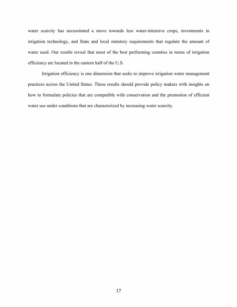
An illustration of irrigation efficiency is provided in Figure 1. The inefficient
representative decision-making unit is initially producing output level 𝑞! using 𝑥!! units of
irrigation water. In Figure 2, OTE is a radial measure where 𝑂𝑇𝐸 = 0𝐵/0𝐴. The minimum
feasible quantity of water needed to produce 𝑞! is denoted by 𝑥!! ; therefore, the maximum
possible reduction in irrigation water is given as 𝑥!! − 𝑥!!; hence, 𝐼𝐸 = 𝑥!! 𝑥!!. The quantity 𝑥!! is
not observed; however, rewriting the latter expression for IE we can get 𝑥!! = 𝐼𝐸 × 𝑥!! .
Therefore, the stochastic production frontier in 4 above can be rewritten as:
5 𝑦!" = 𝛼!! + 𝛼!𝑡 + 𝛽!! ln 𝑥!!"! + 𝛽! ln 𝑥!"#
!
!!!
+ 𝜌! ln 𝑧!"#
!"
!!!
+ 𝑣!"
Note that 𝑥!!"! lies on the frontier, a region that is technically efficient, therefore 𝑢!" = 0. The
economic intuition is that one can obtain a non-radial measure of irrigation water, holding output
and all other inputs constant, and thus establish the extent to which the quantity of irrigation
water applied can be reduced. Thus, a measure of irrigation efficiency can be obtained by
equating expressions (4) and (5) in order to obtain:
6 𝐼𝐸! = 𝑙𝑛𝑥!!"! − 𝑙𝑛𝑥!!" = exp𝑢!"𝛽!!
Results from equation 6 will enable us to establish how efficient DMUs are at using the minimal
possible level of irrigation water. The OTE and IE approach will enable the dual ranking of
counties based on both measures.
13
Results
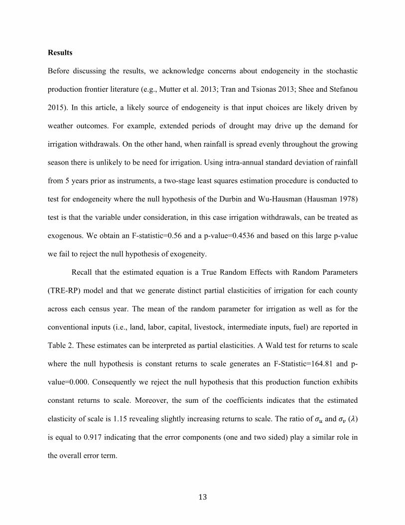
Before discussing the results, we acknowledge concerns about endogeneity in the stochastic
production frontier literature (e.g., Mutter et al. 2013; Tran and Tsionas 2013; Shee and Stefanou
2015). In this article, a likely source of endogeneity is that input choices are likely driven by
weather outcomes. For example, extended periods of drought may drive up the demand for
irrigation withdrawals. On the other hand, when rainfall is spread evenly throughout the growing
season there is unlikely to be need for irrigation. Using intra-annual standard deviation of rainfall
from 5 years prior as instruments, a two-stage least squares estimation procedure is conducted to
test for endogeneity where the null hypothesis of the Durbin and Wu-Hausman (Hausman 1978)
test is that the variable under consideration, in this case irrigation withdrawals, can be treated as
exogenous. We obtain an F-statistic=0.56 and a p-value=0.4536 and based on this large p-value
we fail to reject the null hypothesis of exogeneity.
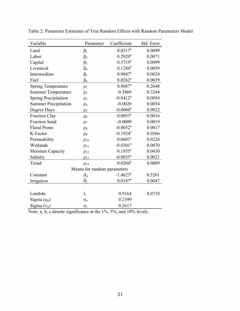
Recall that the estimated equation is a True Random Effects with Random Parameters
(TRE-RP) model and that we generate distinct partial elasticities of irrigation for each county
across each census year. The mean of the random parameter for irrigation as well as for the
conventional inputs (i.e., land, labor, capital, livestock, intermediate inputs, fuel) are reported in
Table 2. These estimates can be interpreted as partial elasticities. A Wald test for returns to scale
where the null hypothesis is constant returns to scale generates an F-Statistic=164.81 and p-
value=0.000. Consequently we reject the null hypothesis that this production function exhibits
constant returns to scale. Moreover, the sum of the coefficients indicates that the estimated
elasticity of scale is 1.15 revealing slightly increasing returns to scale. The ratio of 𝜎! and 𝜎! (𝜆)
is equal to 0.917 indicating that the error components (one and two sided) play a similar role in
the overall error term.
14
The estimates of the weather variables reveal that, on average, spring temperatures (April
to June), spring precipitation (April to June) and the number of degree-days have statistically
significant impacts on the total value of agricultural output. These results indicate that, ceteris
paribus, average spring precipitation has a negative effect whereas average spring temperatures
have a positive impact on total value of agricultural output. On the other hand, an increase in the
number of degree-days (i.e., days with temperatures exceeding 89.4°F) has a negative effect on
total value of output.
Finally, results on the impact of land and soil features on total value of agricultural output
reveal that regions characterized by clay soils, higher levels of soil permeability, and moisture
capacity all result in higher levels of total value of agricultural output. On the other hand, soils
characterized as flood-prone, susceptible to soil erosion (k-factor), wetlands, and saline soils
contribute, ceteris paribus, lead to lower values of agricultural output.
As mentioned earlier, irrigation efficiency is measured as the minimum feasible quantity
of water needed to generate a given level of output at the frontier (Karagiannis et al. 2003). It
involves estimating the maximal possible reduction in irrigation withdrawals while holding all
other inputs constant. The economic intuition being that the usage of irrigation water input can
be progressively scaled back up to a minimal feasible level required for producing a given level
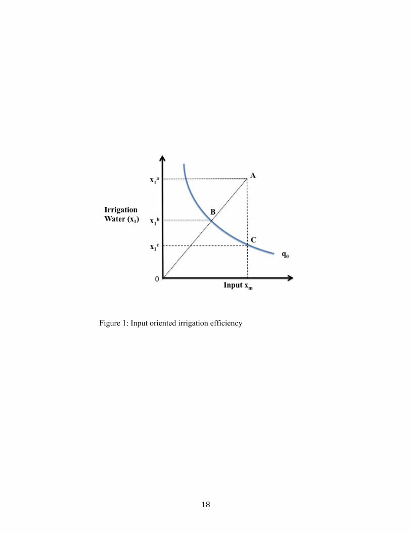
of output. Average irrigation efficiency across all counties is estimated to be 79.4% whereas
average technical efficiency across all counties is estimated to be 81.4%. An illustration of the
kernel densities of irrigation efficiency and technical efficiency is provided in Figure 2. In Table
3, we present results of the best performing Counties based on estimates of irrigation efficiency
for the years 1987, 1992, 1997, 2002, 2007 and 2012. Wilchens (2010) conjectures that counties
that rely heavily on irrigation for their primary water needs are likely to be more efficient than
15
counties that use irrigation water for supplemental purposes. Based on our results, we find no
evidence that this is the case. On the contrary, other than the counties of San Luis Obispo, CA,
Santa Barbara, CA, Tillamook, OR and Cavalier, ND, all the other counties that rank highest in
terms of irrigation efficiency are located in the eastern half of the United States which is
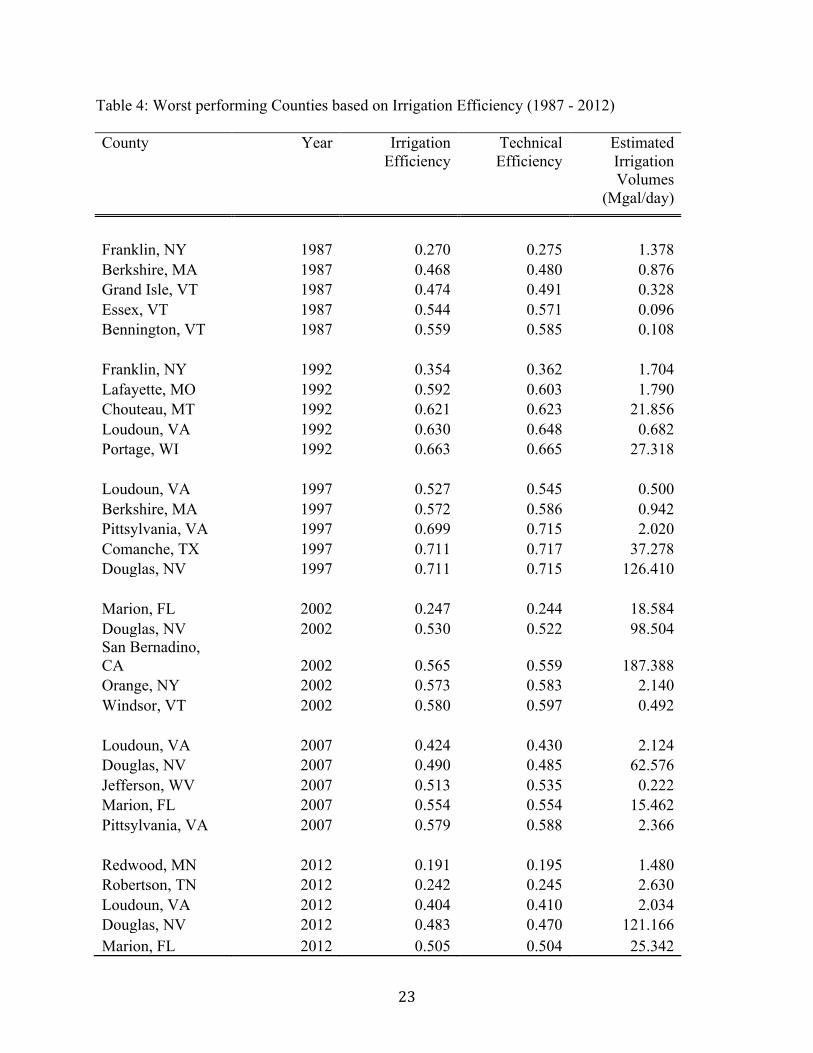
characterized by a farm sector that utilizes irrigation for supplemental needs. In Table 4 we
present results of the worst performing counties, again based on our estimates of irrigation
efficiency. With the exception of San Bernardino, CA, Comanche, TX and Douglas, NV, the
counties that feature on this list are located in the eastern half of the U.S. We also present
technical efficiency estimates alongside the irrigation efficiency estimates. We find that counties
characterized by high levels of irrigation efficiency are also likely to be highly technically
efficient. Conversely, counties that are characterized by low levels of irrigation efficiency are
also technically inefficient.
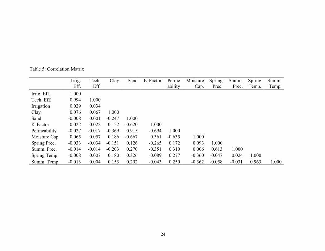
In Table 5 we provide a correlation matrix that illustrates the relationship between
irrigation efficiency, technical efficiency, with some of the environmental factors, such as,
fraction of clay and sand, susceptibility to soil erosion (k-factor), soil permeability, moisture
capacity, spring and summer temperatures, and precipitation. Recall that irrigation efficiency is
defined as the minimum feasible quantity of irrigation water needed to produce a given level of
output. We find irrigation efficiency to be negatively correlated with sand, and soil permeability,
revealing that regions characterized by sandy soils and high levels of soil permeability require
higher volumes of irrigation water than the minimum feasible needed to generate a given level of
output. In addition, we find irrigation efficiency to be negatively correlated with spring and
summer temperatures and precipitation. We surmise that increased levels of spring and summer
temperatures lead to higher levels of evapotranspiration necessitating higher volumes of water
16
than the minimum feasible required. On the other hand, irrigation that is conducted in the
presence of increased precipitation levels is likely to lead to more than minimum feasible levels
required for agricultural output leading to lower levels of irrigation efficiency.
Concluding Remarks
This article uses stochastic production frontier production methods to calculate and evaluate
measures of technical efficiency and irrigation efficiency using a sample of 340 counties of the
top U.S. agricultural counties based on the total value of agricultural sales. Two distinct
approaches are used: an output-oriented technical efficiency approach that radially measures the
efficiency of all inputs used in the production process; as well as a non-radial input-oriented
approach that isolates and measures the efficiency of a single input. The objective is to evaluate
irrigation efficiency across U.S. counties in the presence of climatic variability and diverse
environmental and topographic conditions. Our general findings reveal that irrigation contributes
positively to output. As regards irrigation efficiency, which we define as the minimum feasible
quantity of irrigation water needed to produce a given level of output, we find that irrigation
efficiency averaged 79.4%. On the other hand, technical efficiency averaged 81.4% during the
period of study, 1987-2012. Our findings also reveal irrigation efficiency to be highly correlated
with technical efficiency thus establishing that counties that are technically efficient are also
likely to be characterized by high levels of irrigation efficiency. Some studies have observed that
states in the western half of the U.S. rely on irrigation for their primary water needs whereas in
states located in the eastern half of the country irrigation is mostly supplemental (e.g., Wichelns
2010; Schaible and Aillery 2012). Based on this, we conjecture that counties that are heavily
reliant on irrigation water for their primary needs are likely to be more efficient partly because
17
water scarcity has necessitated a move towards less water-intensive crops, investments in
irrigation technology, and State and local statutory requirements that regulate the amount of
water used. Our results reveal that most of the best performing counties in terms of irrigation
efficiency are located in the eastern half of the U.S.
Irrigation efficiency is one dimension that seeks to improve irrigation water management
practices across the United States. These results should provide policy makers with insights on
how to formulate policies that are compatible with conservation and the promotion of efficient
water use under conditions that are characterized by increasing water scarcity.
18
Figure 1: Input oriented irrigation efficiency
19
Figure 2: Probability density function for technical and irrigation efficiency
0
1
2
3
4
5
6
7
0.15 0.35 0.55 0.75 0.95
probabilitydensityfunction
IrrigationEf6iciency
TechnicalEf6iciency
20
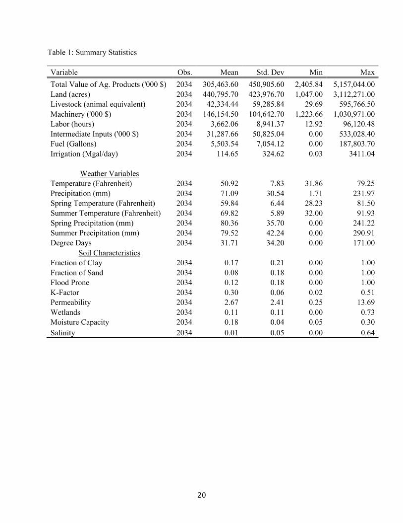
Table 1: Summary Statistics
Variable Obs. Mean Std. Dev Min Max Total Value of Ag. Products ('000 $) 2034 305,463.60 450,905.60 2,405.84 5,157,044.00 Land (acres) 2034 440,795.70 423,976.70 1,047.00 3,112,271.00 Livestock (animal equivalent) 2034 42,334.44 59,285.84 29.69 595,766.50 Machinery ('000 $) 2034 146,154.50 104,642.70 1,223.66 1,030,971.00 Labor (hours) 2034 3,662.06 8,941.37 12.92 96,120.48 Intermediate Inputs ('000 $) 2034 31,287.66 50,825.04 0.00 533,028.40 Fuel (Gallons) 2034 5,503.54 7,054.12 0.00 187,803.70 Irrigation (Mgal/day) 2034 114.65 324.62 0.03 3411.04
2034 50.92 7.83 31.86 79.25 2034 71.09 30.54 1.71 231.97 2034 59.84 6.44 28.23 81.50 2034 69.82 5.89 32.00 91.93 2034 80.36 35.70 0.00 241.22 2034 79.52 42.24 0.00 290.91
Weather Variables Temperature (Fahrenheit) Precipitation (mm) Spring Temperature (Fahrenheit) Summer Temperature (Fahrenheit) Spring Precipitation (mm)Summer Precipitation (mm)Degree Days 2034 31.71 34.20 0.00 171.00
Soil Characteristics Fraction of Clay 2034 0.17 0.21 0.00 1.00 Fraction of Sand 2034 0.08 0.18 0.00 1.00 Flood Prone 2034 0.12 0.18 0.00 1.00 K-Factor 2034 0.30 0.06 0.02 0.51 Permeability 2034 2.67 2.41 0.25 13.69 Wetlands 2034 0.11 0.11 0.00 0.73 Moisture Capacity 2034 0.18 0.04 0.05 0.30 Salinity 2034 0.01 0.05 0.00 0.64
21
Table 2: Parameter Estimates of True Random Effects with Random Parameters Model
Variable Parameter Coefficient Std. Error Land β1 0.0317a 0.0099 Labor β2 0.2920a 0.0071 Capital β3 0.5719a 0.0099 Livestock β4 0.1284a 0.0059 Intermediate β5 0.0847a 0.0024 Fuel β6 0.0262a 0.0039 Spring Temperature ρ1 0.9687a 0.2648 Summer Temperature ρ2 -0.3869 0.3244 Spring Precipitation ρ3 -0.0412a 0.0054 Summer Precipitation ρ4 -0.0020 0.0054 Degree Days ρ5 -0.0060a 0.0022 Fraction Clay ρ6 0.0053a 0.0016 Fraction Sand ρ7 -0.0009 0.0019 Flood Prone ρ8 -0.0052a 0.0017 K-Factor ρ9 -0.1924a 0.0366 Permeability ρ10 0.0601a 0.0226 Wetlands ρ11 -0.0301a 0.0070 Moisture Capacity ρ12 0.1955a 0.0430 Salinity ρ13 -0.0035c 0.0021 Trend ρ14 0.0204a 0.0009
Means for random parameters Constant 𝛼! -1.4623a 0.5201 Irrigation 𝜃! 0.0187a 0.0047
Lambda λ 0.9164 0.0718 Sigma (uit) σu 0.2399 Sigma (vit) σv 0.2617
Note: a, b, c denote significance at the 1%, 5%, and 10% levels.
22
Table 3: Best performing Counties based on Irrigation Efficiency (1987 - 2012)
County Year Irrigation Efficiency
Technical Efficiency
Estimated Irrigation Volumes
(Mgal/day)
Union, NC 1987 0.878 0.906 3.080 York, ME 1987 0.870 0.892 0.910 Sheboygan, WI 1987 0.869 0.892 1.246 Duplin, NC 1987 0.864 0.894 4.172 Piscataquis, ME 1987 0.864 0.879 0.128
Essex, VT 1992 0.882 0.891 0.090 Union, NC 1992 0.880 0.913 5.380 Frederick, MD 1992 0.876 0.918 8.878 Rockingham, VA 1992 0.875 0.908 6.176 Cavalier, ND 1992 0.874 0.888 0.168
Monroe, WI 1997 0.929 0.963 1.314 San Luis Obispo, CA 1997 0.892 0.897 161.444 Santa Barbara, CA 1997 0.891 0.908 286.252 Mills, IA 1997 0.889 0.909 0.736 Essex, VT 1997 0.889 0.894 0.058
Morris, NJ 2002 0.899 0.922 1.210 Frederick, MD 2002 0.886 0.912 2.382 Tillamook, OR 2002 0.882 0.915 5.194 Rockingham, VA 2002 0.878 0.908 2.672 Cavalier, ND 2002 0.875 0.882 0.028
Jo Daviess, IL 2007 0.918 0.948 1.474 Fayette, KY 2007 0.907 0.938 1.578 Middlesex, MA 2007 0.904 0.930 4.266 Frederick, MD 2007 0.899 0.932 2.342 Cavalier, ND 2007 0.895 0.902 0.066
Wilkin, MN 2012 0.972 0.962 0.170 Cavalier, ND 2012 0.902 0.906 0.056 Traverse, MN 2012 0.895 0.904 0.152 Essex, VT 2012 0.894 0.901 0.122 Union, NC 2012 0.888 0.917 2.966
23
Table 4: Worst performing Counties based on Irrigation Efficiency (1987 - 2012)
County Year Irrigation Efficiency
Technical Efficiency
Estimated Irrigation Volumes
(Mgal/day)
Franklin, NY 1987 0.270 0.275 1.378 Berkshire, MA 1987 0.468 0.480 0.876 Grand Isle, VT 1987 0.474 0.491 0.328 Essex, VT 1987 0.544 0.571 0.096 Bennington, VT 1987 0.559 0.585 0.108
Franklin, NY 1992 0.354 0.362 1.704 Lafayette, MO 1992 0.592 0.603 1.790 Chouteau, MT 1992 0.621 0.623 21.856 Loudoun, VA 1992 0.630 0.648 0.682 Portage, WI 1992 0.663 0.665 27.318
Loudoun, VA 1997 0.527 0.545 0.500 Berkshire, MA 1997 0.572 0.586 0.942 Pittsylvania, VA 1997 0.699 0.715 2.020 Comanche, TX 1997 0.711 0.717 37.278 Douglas, NV 1997 0.711 0.715 126.410
Marion, FL 2002 0.247 0.244 18.584 Douglas, NV 2002 0.530 0.522 98.504 San Bernadino, CA 2002 0.565 0.559 187.388 Orange, NY 2002 0.573 0.583 2.140 Windsor, VT 2002 0.580 0.597 0.492
Loudoun, VA 2007 0.424 0.430 2.124 Douglas, NV 2007 0.490 0.485 62.576 Jefferson, WV 2007 0.513 0.535 0.222 Marion, FL 2007 0.554 0.554 15.462 Pittsylvania, VA 2007 0.579 0.588 2.366
Redwood, MN 2012 0.191 0.195 1.480 Robertson, TN 2012 0.242 0.245 2.630 Loudoun, VA 2012 0.404 0.410 2.034 Douglas, NV 2012 0.483 0.470 121.166 Marion, FL 2012 0.505 0.504 25.342
23
Table 5: Correlation Matrix
Irrig. Eff.
Tech. Eff.
Clay Sand K-Factor Permeability
Moisture Cap.
Spring Prec.
Summ. Prec.
Spring Temp.
Summ. Temp.
Irrig. Eff. 1.000 Tech. Eff. 0.994 1.000 Irrigation 0.029 0.034 Clay 0.076 0.067 1.000
Sand -0.008 0.001 -0.247 1.000 K-Factor 0.022 0.022 0.152 -0.620 1.000
Permeability -0.027 -0.017 -0.369 0.915 -0.694 1.000 Moisture Cap. 0.065 0.057 0.186 -0.667 0.361 -0.635 1.000 Spring Prec. -0.033 -0.034 -0.151 0.126 -0.265 0.172 0.093 1.000 Summ. Prec. -0.014 -0.014 -0.203 0.270 -0.351 0.310 0.006 0.613 1.000
Spring Temp. -0.008 0.007 0.180 0.326 -0.089 0.277 -0.360 -0.047 0.024 1.000 Summ. Temp. -0.013 0.004 0.153 0.292 -0.043 0.250 -0.362 -0.058 -0.031 0.963 1.000
24
25
References
Adams, R.M., R.A. Fleming, C. Chang, B.A. McCarl, and C. Rosenzweig. 1995. A
Reassessment of the Economic Effects of Global Climate Change on U.S. Agriculture.
Climatic Change 30(2): 147-167.
Aigner, D. J., C. A. K. Lovell, and P. Schmidt. 1977. Formulation and Estimation of Stochastic
Frontier Production Function Models. Journal of Econometrics 6(1): 21-37.
Chakraborty, K., S. Misra, and P. Johnson. 2002. Cotton Farmers’ Technical Efficiency:
Stochastic and Nonstochastic Production Function Approaches. Agricultural and Resource
Economics Review 31(2): 211-220.
Clemmens, A. J., R. G. Allen, and C. M. Burt. 2008. Technical Concepts Related to
Conservation of Irrigation and Rainwater in Agricultural Systems. Water Resources Research
44(7): 1-16.
Daly, C., J.I. Smith, and K.V. Olson. 2015. Mapping Atmospheric Moisture Climatologies
Across Conterminous United States. PloS One 10(10): e0141140.
doi:10.1371/journal.pone.0141140.
Daly, C., M.P. Widrlechner, M.D. Halbleib, J.I. Smith, and W.P. Gibson. 2012. Development of
a New USDA Plant Hardiness Zone Map for the United States. Journal of Applied
Meteorology and Climatology 51: 242-264.
Daly, C., M. Halbleib, J.I. Smith, W.P. Gibson, M.K. Doggett, G.H. Taylor, J. Curtis, and P.A.
Pasteris. 2008. Physiographically-sensitive Mapping of Temperature and Precipitation Across
the Conterminous United States. International Journal of Climatology 28: 2031-2064.
26
Deschenes, O., and M. Greenstone. 2007. The Economic Impacts of Climate Change: Evidence
from Agricultural Output and Random Fluctuations in Weather. American Economic Review
97(1): 354-385.
Evans, R.G., and E.J. Sadler. 2008. Methods and Technologies to Improve Efficiencies of Water
Use. Water Resources Research 44(7): 1-15.
Greene, W.H. 2012. Econometric Analysis. Prentice Hall (seventh edition).
Greene, W.H. 2005a. Reconsidering Heterogeneity in Panel Data Estimators of the Stochastic
Frontier Model. Journal of Econometrics 126 (2): 269-303.
Greene, W.H. 2005b. Fixed and Random Effects in Stochastic Frontier Models. Journal of
Productivity Analysis 23(1): 7-32.
Hatfield, J., G. Takle, R. Grotjahn, P. Holden, R.C. Izaurralde, T. Mader, E. Marshall, and D.
Liverman. 2014: Ch. 6: Agriculture. Climate Change Impacts in the United States: The Third
National Climate Assessment, J. M. Melillo, Terese (T.C.) Richmond, and G. W. Yohe, (Eds),
U.S. Global Change Research Program, 150-174. doi:10.7930/J02Z13FR.
Karagiannis, G., V. Tzouvelekas, and A. Xepapadeas. 2003. Measuring Irrigation Water
Efficiency with a Stochastic Production Frontier. Environmental and Resource Economics 26:
57-72.
Kopp, R. J. 1981. The Measurement of Productive Efficiency: A Reconsideration. Quarterly
Journal of Economics 96: 477-503.
Lilienfeld, A., and M. Asmild. 2007. Estimation of Excess Water Use in Irrigated Agriculture: A
Data Envelopment Analysis Approach. Agricultural Water Management 94: 73-82.
McGuckin, J. T., N. Gollehon, and S. Ghosh. 1992. Water Conservation in Irrigated Agriculture:
A Stochastic Production Frontier Model. Water Resources Research 28(2): 305-312.
27
Meeusen, W., and J. van den Broeck. 1977. Efficiency Estimation from Cobb-Douglas
Production Functions with Composed Error. International Economic Review 18(2): 435-444.
Mendelsohn, R., W. D. Nordhaus, and D. Shaw. 1994. The Impact of Global Warming on
Agriculture: A Ricardian Analysis. American Economic Review 84(4): 753-771.
Mendelsohn, R., and A. Dinar. 2003. Climate, Water, and Agriculture. Land Economics 79(3):
328-341.
Mutter, R.L., W.H. Greene, W. Spector, M.D. Rosko, and D.B. Mukamel. 2013. Investigating
the Impact of Endogeneity on Inefficiency Estimates in the Application of Stochastic Frontier
Analysis to Nursing Homes. Journal of Productivity Analysis 39(2): 101-110.
Njuki, E., and B.E. Bravo-Ureta. 2016. Does Irrigation Improve Agricultural Productivity?
Examining Irrigation Patterns in U.S. Agriculture. Working Paper. Zwick Center for Food and
Resource Policy.
O’Donnell, C.J. 2016. Using Information About Technologies, Markets and Firm Behaviour to
Decompose a Proper Productivity Index. Journal of Econometrics 190(2): 328-340.
O’Donnell, C.J. 2012. An Aggregate Quantity Framework for Measuring and Decomposing
Productivity Change. Journal of Productivity Analysis 38(3): 255-272.
Reinhard, S., C. A. K. Lovell, and G. Thijssen. 1999. Econometric Estimation of Technical and
Environmental Efficiency: An Application to Dutch Dairy Farms. American Journal of
Agricultural Economics 81(1): 44-60.
Schaible, G. D. and M. P. Aillery. 2012. Water Conservation in Irrigated Agriculture: Trends and
Challenges in the Face of Emerging Demands. EIB-99. U.S. Department of Agriculture,
Economic Research Service, Washington, D.C.
28
Scheierling, S. M., David O. Treguer, J. F. Booker, and E. Decker. 2014. How to Assess
Agricultural Water Productivity? Looking for Water in the Agricultural Productivity and
Efficiency Literature. Policy Research Working Paper 6982. World Bank, Washington, DC.
Schlenker, W., W. M. Hanneman, and A. C. Fisher. 2005. Will U.S. Agriculture Really Benefit
from Global Warming? Accounting for Irrigation in the Hedonic Approach. American
Economic Review 95(1): 395-406.
Schlenker, W., W. M. Hanneman, and A. C. Fisher. 2006. The Impact of Global Warming on
U.S. Agriculture: An Econometric Analysis of Optimal Growing Conditions. Review of
Economics and Statistics 88(1): 113-125.
Schlenker, W., and M. J. Roberts. 2009. Nonlinear Temperature Effects Indicate Severe
Damages to U.S. Crop Yields under Climate Change. Proceedings of the National Academy of
Sciences 106(37): 15594-15598.
Seckler, D., D. Molden, and R. Sakthivadivel. 2003. The Concept of Efficiency in Water
Resources Management and Policy. In: Kijne, J.W., R. Barker, and D. Molden (Eds.), Water
Productivity in Agriculture: Limits and Opportunities for Improvement. CABI Publishing and
International Water Management Institute, Wallingford, UK/Colombo, Sri Lanka.
Shee, A., and S.E. Stefanou. 2015. Endogeneity Corrected Stochastic Production Frontiers and
Technical Efficiency. American Journal of Agricultural Economics 97(3): 939-952
Shephard, R. 1970. The Theory of Cost and Production Functions. Princeton University Press,
Princeton.
Tsionas, E. G., and S. C. Kumbhakar. 2014. Firm Heterogeneity, Persistent and Transient
Technical Inefficiency: A Generalized True Random-Effects Model. Journal of Applied
Econometrics 29(1): 110-132.
29
U.S. Department of Agriculture. 2014. Strategic Plan 2014-2018. USDA, Washington DC.
Weinberg, M., C. L. Kling, and J. E. Wilen. 1993. Water Markets and Water Quality. American
Journal of Agricultural Economics 75: 278-291.
Wichelns, D. 2010. Agricultural Water Pricing: United States. Sustainable Management of
Water Resources in Agriculture. OECD.
Wu, S., S. Devadoss, and Y. Lu. 2003. Estimation and Decomposition of Technical Efficiency
for Sugarbeet Farms. Applied Economics 35: 471-484.
Zilberman, D. 2014. The Economics of Sustainable Development. American Journal of
Agricultural Economics 96(2): 385-396.