classification, multiple hypothesis testing and … · dipartimento: matematica e applicazioni...
TRANSCRIPT
DOTTORATO DI RICERCA
in
SCIENZE COMPUTAZIONALI ED INFORMATICHE
Ciclo XVIII
Consorzio tra Universita di Catania, Universita di Napoli Federico II,
Seconda Universita degli studi di Napoli, Universita di Palermo, Universita di Salerno
SEDE AMMINISTRATIVA: UNIVERSITA DI NAPOLI FEDERICO II
AUTORE
LUISA CUTILLO
CLASSIFICATION, MULTIPLE HYPOTHESIS TESTING
AND WAVELET THRESHOLDING PROCEDURES
WITH APPLICATIONS
TESI DI DOTTORATO DI RICERCA

UNIVERSITA DEGLI STUDI DI NAPOLI
FEDERICO II
Autore: Luisa Cutillo
Titolo: Classification, Multiple Hypothesis Testing and Wavelet
Thresholding procedures with Applications
Dipartimento:Matematica e Applicazioni ’R.Caccioppoli’
Tesi diDottorato Anno: 2005
Firma dell’autore
ii

To Luigi and Angela
iii

iv

Table of Contents
Table of Contents v
Acknowledgements ix
Introduzione 1
Introduction 5
1 Classification Theory 91.1 General framework . . . . . . . . . . . . . . . . . . . . . . . . . . . . . . 101.2 Statistical Decision theory . . . . . . . . . . . . . . . . . . . . . . . . . . 121.3 Parametric discriminant analysis . . . . . . . . . . . . . . . . . . . . . . . 15
1.3.1 Estimation of the parameters . . . . . . . . . . . . . . . . . . . . 161.3.2 Linear discriminant analysis . . . . . . . . . . . . . . . . . . . . . 171.3.3 Quadratic discriminant Analysis . . . . . . . . . . . . . . . . . . . 18
1.4 Non parametric discriminant analysis . . . . . . . . . . . . . . . . . . . . 191.4.1 Principal component discriminant analysis . . . . . . . . . . . . . 241.4.2 Independent components discriminant analysis . . . . . . . . . . . 26
1.5 Local Discriminant methods for image classification . . . . . . . . . . . . 281.6 Notations and Assumptions . . . . . . . . . . . . . . . . . . . . . . . . . . 311.7 Local priors . . . . . . . . . . . . . . . . . . . . . . . . . . . . . . . . . . 34
1.7.1 Local voting priors . . . . . . . . . . . . . . . . . . . . . . . . . . 351.7.2 Local frequency priors . . . . . . . . . . . . . . . . . . . . . . . . 361.7.3 Local integrated priors . . . . . . . . . . . . . . . . . . . . . . . . 361.7.4 Local nested priors . . . . . . . . . . . . . . . . . . . . . . . . . . 37
1.8 Asymptotics . . . . . . . . . . . . . . . . . . . . . . . . . . . . . . . . . . 381.8.1 Local voting priors . . . . . . . . . . . . . . . . . . . . . . . . . . 38
v
1.8.2 Local frequency priors . . . . . . . . . . . . . . . . . . . . . . . . 391.8.3 Local integrated priors . . . . . . . . . . . . . . . . . . . . . . . . 391.8.4 Local nested priors . . . . . . . . . . . . . . . . . . . . . . . . . . 401.8.5 Iterations . . . . . . . . . . . . . . . . . . . . . . . . . . . . . . . 40
2 Multiple Hypothesis Testing 412.1 General Framework . . . . . . . . . . . . . . . . . . . . . . . . . . . . . . 422.2 Type I Error Rates . . . . . . . . . . . . . . . . . . . . . . . . . . . . . . . 44
2.2.1 Strong and Weak control . . . . . . . . . . . . . . . . . . . . . . . 462.3 Error Controlling Procedures . . . . . . . . . . . . . . . . . . . . . . . . . 47
2.3.1 FWER andFDR Controlling Procedures . . . . . . . . . . . . . 482.4 Bootstrap estimation of the null distribution . . . . . . . . . . . . . . . . . 492.5 Bayesian testing . . . . . . . . . . . . . . . . . . . . . . . . . . . . . . . . 502.6 Bayesian multiple hypothesis testing . . . . . . . . . . . . . . . . . . . . . 52
2.6.1 MAP multple testing procedure . . . . . . . . . . . . . . . . . . . 532.6.2 Connections with frequentist procedures and choice of the priors . 552.6.3 Custom normal model . . . . . . . . . . . . . . . . . . . . . . . . 562.6.4 Possible extension and future work . . . . . . . . . . . . . . . . . 58
3 Wavelet Filtering of Noisy Signals 593.1 Mathematical background . . . . . . . . . . . . . . . . . . . . . . . . . . 603.2 Advantages of wavelets . . . . . . . . . . . . . . . . . . . . . . . . . . . . 653.3 The statistical problem . . . . . . . . . . . . . . . . . . . . . . . . . . . . 673.4 Bayes rules and wavelets . . . . . . . . . . . . . . . . . . . . . . . . . . . 693.5 Larger posterior mode (LPM) wavelet thresholding . . . . . . . . . . . . . 71
3.5.1 Derivation of the thresholding rule . . . . . . . . . . . . . . . . . 723.5.2 Exact risk properties of LPM rules . . . . . . . . . . . . . . . . . . 76
3.6 Generalizations . . . . . . . . . . . . . . . . . . . . . . . . . . . . . . . . 773.6.1 Model 1: exponential prior on unknown variance. . . . . . . . . . . 783.6.2 Model 2: inverse gamma prior on unknown variance. . . . . . . . . 80
3.7 Conclusions and future works . . . . . . . . . . . . . . . . . . . . . . . . 81
4 Numerical Experiments for Discriminant Analysis 834.1 Multispectral cloud detection: general problem . . . . . . . . . . . . . . . 83
4.1.1 Classification methods considered . . . . . . . . . . . . . . . . . . 854.1.2 Case studies . . . . . . . . . . . . . . . . . . . . . . . . . . . . . . 864.1.3 Results . . . . . . . . . . . . . . . . . . . . . . . . . . . . . . . . 87
vi

4.2 Simulation of Local discriminant methods . . . . . . . . . . . . . . . . . . 884.2.1 Real data . . . . . . . . . . . . . . . . . . . . . . . . . . . . . . . 914.2.2 Conclusions . . . . . . . . . . . . . . . . . . . . . . . . . . . . . . 92
5 Application of multiple testing procedures to DNA microarray data 1055.1 What is a microarray ? . . . . . . . . . . . . . . . . . . . . . . . . . . . . 1065.2 Experimental Design . . . . . . . . . . . . . . . . . . . . . . . . . . . . . 1085.3 Expression Ratio . . . . . . . . . . . . . . . . . . . . . . . . . . . . . . . 1095.4 Normalization . . . . . . . . . . . . . . . . . . . . . . . . . . . . . . . . . 110
5.4.1 Single slide data displays . . . . . . . . . . . . . . . . . . . . . . . 1105.4.2 Within slide normalization . . . . . . . . . . . . . . . . . . . . . . 1115.4.3 Global normalization . . . . . . . . . . . . . . . . . . . . . . . . . 1115.4.4 Intensity dependent normalization . . . . . . . . . . . . . . . . . . 1125.4.5 Within print tip group normalization . . . . . . . . . . . . . . . . . 1135.4.6 Scale normalization . . . . . . . . . . . . . . . . . . . . . . . . . . 1135.4.7 Multiple slide normalization . . . . . . . . . . . . . . . . . . . . . 114
5.5 Yeast experiment . . . . . . . . . . . . . . . . . . . . . . . . . . . . . . . 1145.5.1 Experiment description . . . . . . . . . . . . . . . . . . . . . . . . 1145.5.2 Methods . . . . . . . . . . . . . . . . . . . . . . . . . . . . . . . 116
6 LPM: simulations, comparisons and real life example 1196.1 Selection of hyperparameters . . . . . . . . . . . . . . . . . . . . . . . . . 1196.2 Simulations and comparisons . . . . . . . . . . . . . . . . . . . . . . . . 1266.3 An example in atomic force microscopy . . . . . . . . . . . . . . . . . . . 129
A 133A.1 Proof of Lemma (3.6.1) . . . . . . . . . . . . . . . . . . . . . . . . . . . . 133A.2 Proof of lemma (3.6.2) . . . . . . . . . . . . . . . . . . . . . . . . . . . . 135A.3 Selection of hyperparametersα andβ in Model 2. . . . . . . . . . . . . . . 138
Bibliography 139
vii

viii

Acknowledgements
I would like to thank Umberto Amato, my supervisor, for his many suggestions and con-stant support during this research. I am also thankful to Claudia Angelini for her guidancethrough the early years of confusion.
I am gratefull to Professor Brani Vidakovic, who expressed his interest in my work andsupplied me with some of his recent works. Yoon Young shared with me her knowledgeof statistical analysis and provided many useful references and friendly encouragement. Ishould also mention the support from University “Frederico II” that, under the programmobilit di breve durata, gave me the opportunity of visiting the Georgia Institute of Thec-nology, Atlanta.
Of course, I am grateful to my husband Luigi for his patience andlove. Without himthis work would never have come into existence (literally).
Finally, I wish to thank the following friends: Annamaria for her sincere friendship,Francesca and Italia for bearing me in their work place, Monica for her cakes, Alba forher encouragements, Angela, Claudia, Mariarosaria and Woulla for having lunch with meeveryday and my sister Angela.... because she asked me to.
Napoli, Italia Luisa CutilloNovember 30, 2005
ix

Introduzione
Lo sviluppo delle metodologie statitistiche per l’analisi datie generalmente collegato a pro-
gressi ottenuti in altri campi scientifici. Da un lato l’analisi statisticae spesso indirizzata a
problemi reali, di conseguenza, il miglioramento delle metodologie nasce dall’esigenza di
fornire una soluzione sempre piu accurata ed efficiente a problemi specifici. D’altro canto
accade anche che le procedure statistiche siano prima esplorate in ambito teorico e succes-
sivamente testate prima in simulazione e quindi su dati reali. In quest’ottica, lo scopo di
questo lavoroe quello di mostrare sia come problemi reali possano essere efficientemente
risolti mediante tecniche statistiche, sia come modelli statistici teorici possano essere adatti
a descrivere problemi reali.
Nella pratica spesso ci troviamo a dover analizzare grandi moli di dati con molte dimen-
sioni. Conseguentemente siamo costretti ad affrontare il problema della dimensionalita.
Esistono differenti approcci statistici per fronteggiare questa difficolta. Ad esempio, data
una immagine satellitare dell’Europa ad una risoluzione di 800x600 pixel, consideriamo
un insieme di dati costituito dalle radianze, misurate su 15 canali, associate ad ogni pixel.
Supponiamo lo scopo sia quello di classificare ciascun pixel come appartenete ad una di
1

2
due classi predefinite, come ad esempio nuvoloso e sereno. Prendendo a modello il pro-
cesso cognitivo della nostra mente, abbiamo bisogno di estrarre le informazioni dai dati,
cioe dobbiamo poter individuare strutture dati significative e di piccole dimensioni, nello
spazio delle ossevazioni. Esiste un’ampia classe di tecniche statistiche mediante le quali il
problema della dimensionalita puo essere gestito, come ad esempio l’analisi delle compo-
nenti principali utilizzate in combinazione con i metodi kernel, o l’analisi delle componenti
indipendenti. Illustreremo la teoria statistica della classificazione supervisionata e discute-
remo alcuni aspetti riguardanti la classificazione localizzata di immagini.
Un altro esempio di dati di grandi dimensioni proviene dal recente e interessante avvento
della tecnologia dei microarray. Negli ultimi anni i DNA microarray sono diventati uno
strumento base per la ricerca biologica. Il diffondersi di questa tecnologia ha potenziato la
ricerca nell’ambito della genomica funzionale, consentendo il monitoraggio dei profili di
espressione di migliaia di geni (anche dell’intero genoma) contemporaneamente. La grande
mole di dati generati da questo tipo di esperimenti ha permesso lo sviluppo di nuove in-
teressanti metodologie statistiche. Conseguentemente l’analisi di dati da DNA microarray
costituisce un’applicazione Biostatistica e Bioinformatica di crescente interesse. Oggetto
della nostra analisi sara lo sviluppo di una tecnica per l’individuazione dei pochi geni dif-
ferenzialmente espressi in un particolare contesto sperimentale. Il problema verra formu-
lato in termini di test di ipotesi multipla e verranno anche illustrate tutte le fasi dell’analisi
dei dati da DNA microarray.
Come ultimo esempio, consideriamo un esperimento in cui lo scopoe analizzare un

3
segnale digitale proveniente da una strumentazione elettronica a partire da migliaia di
misurazioni empiriche. Anche in condizioni sperimentali ottimali, le misurazioni di cui
disponiamo saranno affette da errore. L’analisi di tali segnalie riconducibile al problema
di ricostruzione di un segnale contaminato da rumore. Questo probelmae noto sotto diversi
nomi (denoising, filtering, smoothing, regressionetc.) a seconda del campo scientifico in
cui e affrontato. In letteratura sono state proposte differenti soluzioni mediante splines, fun-
zioni kerel, serie di Fourier e wavelet. In questa sede affronteremo il problema nell’ottica
della regressione non parametrica e presenteremo come soluzione alcune regole di wavelet
thresholding. La scelta di utilizzare la teoria delle wavelet deriva principalmente dalla pos-
sibilita di ottenere una ricostruzione ottimale del segnale originale anche nel caso in cui
quest’ultimo sia fortemente irregolare. Questo risultato non puo essere ottenuto mediante
nessun altro stimatore lineare e deriva dalla proprieta delle basi wavelet di approssimare un
vasto insieme di spazi funzionali.
La tesi e organizzata come segue. Nel Capitolo 1 viene affrontato il problema della
classificazione supervisionata con lo scopo di risolvere il problema della classificazione
di immagini. Vengono passati in rassegna alcuni metodi standard ed in particolaree de-
scritto il problema della classificazione di immagini mediante tecniche locali. I risultati
dell’applicazione delle metodologie proposte a dati reali e simulati verranno poi presentati
nel Capitolo 4. Nel Capitolo 2 viene introdotto il problema dei test di ipotesi multipla con
l’obiettivo di fornire uno strumento di analisi di dati da cDNA microarray. Viene fornita
una prospettiva critica dell’impostazione Bayesiana e frequentista del problema e sono de-
scritti punti di forza, di debolezza e di contatto tra le due filosofie. L’applicazione a dati

4
reali da cDNA microarray delle metodologie discusse sara presentata nel Capitolo 6. Nel
Capitolo 3 sono analizzate nel dominio wavelet alcune regole di thresholding indotte da
una variazione del principio bayesiano delMaximum A Posteriori(MAP). Le regole MAP
sono azioni Bayesiane che massimizzano la probabilita a posteriori. La metodologia pro-
posta risulta essere di tipo thersholding ede caratterizzata dalla proprieta di selezionare la
moda della probabilita a posteriori che risulta essere piu grande in valore assoluto, da cui il
nomeLarger Posterior Mode(LPM). Forniamo un’analisi del rischio associato alla regola
LPM e mostriamo come le sue prestazioni della regola LPM sono competitive con quelle
di tecniche di letteratura. Il Capitolo 6 presenta infine una discussone sulla scelta degli
iperparametri, uno studio in simulazione della rregola LPM ed una sua applicazione ad un
problema reale.
Questo lavoroe stato svolto durante la mia attivita di ricerca presso l’Istituto per le
Applicazioni del Calcolo Mauro Picone (IAC) , sezione di Napoli. L’interesse all’analisi dei
dati da DNA microarraye nato da una collaborazione con il Telethon Institute of Genetic
and Medicine (TIGEM) e con il Policlinico di Napoli, dove sono stati fisicamente effettuati
gli esperimenti sui DNA microarray .
La parte finale della tesie stata svolta durante il mio periodo di ricerca presso il Georgia
Institute of Technology, Atlanta, Georgia.

Introduction
Development in the field of statistical data analysis is often related to advancements in other
fields to which statistical methods are fruitfully applied. In fact statistical analysis is often
addressed to real problems and methodological improvements are consequently motivated
by the search for the solution of a specific problem. The other way round, sometimes statis-
tical concepts are first theoretically investigated and then applied to simulated or real data
for the development of new techniques. The aim of this work is to show how different real
world problems can be solved efficiently by statistical techniques, and simultaneously to
show how theoretical statistical models can fit real data problems.
In real world problems we frequently face with large sets of high-dimensional data, and as
a consequence, with the problem of dimensionality. This problem can be approached in
different ways. As an example, consider a satellite image of Europe made of 800 x 600
pixel, and suppose we have radiance measures from 15 channels associated to each pixel.
Suppose our purpose is to classify each pixel as coming from two different predefined
classes, e.g. cloudy or non cloudy. As the human brain does in everyday perception, we
need then to find meaningful low-dimensional structures hidden in the high-dimensional
observation space. There is a wide class of statistical techniques, by which this problem
can be handled, as principal component analysis, in combination with Kernel methods, or
5

6
independent components discriminant analysis. We will illustrate the statistical theory of
supervised classification and discuss some features regarding localized classification of im-
ages.
Another example of very fashionable high dimensional dataset is microarray data. In a few
years, DNA microarray technology has become a basic tool in biological research. The
growth of this technology has empowered researchers in functional genomics to monitor
gene expression profiles, thousands of genes (even the entire genome) at a time. As a
consequence, the large volume of data generated by these experiments has created an op-
portunity for some very interesting statistical works. For this reasons DNA microarray data
analysis is one of the fastest growing area of applications in Biostatistics and Bioinformat-
ics. We will focus on the problem of finding differentially expressed genes, formulating it
in terms of multiple hypothesis testing. We will illustrate the statistical issues involved at
the various stages of the analysis on real datasets from DNA microarray experiments.
As last example of high dimensional real dataset suppose we have thousands of empiri-
cal measurements of a signal. Even in the best experimental conditions the measurements
will be contaminated by noise, nevertheless the aim is to recover the underlaying unknown
signal. This problem is known under different names (denoising, filtering, smoothing, re-
gressionetc.) according to the scientific field where it is formulated. Different solutions
have been formulated in terms of spline smoothing, kernel estimation, Fourier or wavelet
expansion. We will state the problem in the context of non-parametric regression and will
discuss solutions provided by wavelet thresholding rules. It can be shown that when the un-
derlaying signal is regular and spatially homogeneous, all these methods are asymptotically
equivalent but, for an irregular non homogeneous signal, the wavelet non linear estimation
7
is asymptotically optimal and similar results cannot be achieved by any other linear method.
This happens because wavelet basis can characterize a wide range of functional spaces.
The present thesis is organized as follows. In Chapter 1 we deal with the problem of
supervised classification having in mind the problem of image classification. We review
some of the classical statistical methods for pattern recognition, introduce the problem of
localized classification of images and propose new localized discriminant analysis meth-
ods. Applications of the proposed methodology to simulated and real data, will be provided
in Chapter 4. In Chapter 2 we introduce the statistical problem of multiple hypothesis test-
ing with the target of analyzing cDNA microarray data. We review the guiding lines of
frequentist and Bayesian approach to multiple hypothesis testing, describing strength and
weakness of the two philosophies and trying to find some connections between them. The
application of the described methods to a genetic microarray data experiment is provided
in Chapter 6. In Chapter 3 we explore the thresholding rules in the wavelet domain induced
by a variation of the BayesianMaximum A Posteriori(MAP) principle. The MAP rules are
Bayes actions that maximize the posterior. The proposed rule is thresholding and always
picks the mode of the posterior larger in absolute value, thus the nameLarger Posterior
Mode(LPM). We show that the introduced shrinkage performs comparably to several pop-
ular shrinkage techniques. The exact risk properties of the thresholding rule are explored.
Comprehensive simulations and comparisons are provided in Chapter 6 which also contains
discussion on the selection of hyperparameters and a real-life application of the introduced
shrinkage.

8
The present work was done during my research activity at the Istituto per le Appli-
cazioni del Calcolo ”Mauro Picone” (IAC) in Naples. The interest on microarrays data was
motivated by a collaboration with the Telethon Institute of Genetic and Medicine (TIGEM)
and the Policlinico of Naples, where the biological experiments were carried out.
The last part of this work was done during a visiting period at the Georgia Institute of
Technology (GATECH), in Atlanta, U.S.A.
Chapter 1
Classification Theory
Introduction
In this Chapter we deal with the problem of supervised classification. We review some
of the classical statistical methods for pattern recognition, introduce the problem of local
classification of images and propose new local discriminant methods. Application of the
proposed methodology to simulated and real data, along with suggestions for future work,
would be provided in Chapter 4. Some of the results showed in this Chapter were presented
at theIEEE Goldconference (Naples, 2004) and at theCLADAGmeeting (Parma, 2005).
The Chapter is organized as follows. The first two sections are a brief introduction to
the statistical problem of pattern classification. Sections 3 and 4 describe respectively
some parametric and non parametric approach to supervised classification. Sections 5 and
6 are devoted to the problem of local discriminant analysis and proposals for new local
discriminant methods are discussed in Sections 7 and 8.
9

10
1.1 General framework
Building pattern recognition systems would be very useful in solving myriad of nowadays
problems like fingerprint identification, speech recognition and DNA sequence identifica-
tion. It is amazing to think that humans are used to classify data received from senses
quite immediately and unconsciously. For example most of humans can recognize shapes
by touching, foods by tasting, faces by watching, can detect a specific illness or identify
different types of car. Of course it is crucial for science progress to automatize the hu-
man decision making process so to perform some of these tasks faster, more cheaply or
accurately. One characteristic of human pattern recognition is that it is learnt but learning
involves a teacher. If we try different unlabelled cups of tea we could discover that there
are different groupings and that one group has a green color, but again we need a teacher
to tell us that the common factor is that they were made by the same tea leaves. When the
target of pattern recognition is the discovering of new groupings, it is called unsupervised.
Otherwise, learning from a given set of labelled examples, the training set, in order to clas-
sify future examples is called supervised pattern recognition. We will be only concerned
with supervised pattern recognition. We will assume we are given a finite set of classes and
that a teacher can tell us the correct class label for each pattern in a training set. We could
imagine a pattern recognition system like a machine, called classifier, that takes in input
some measurements of the data, known as features, and tells in output whether the example
is from one of the known classes or not. In statistical pattern recognition, there isn’t any
assumption about the structure of the classifier but it is learnt from data. The training set is
regarded as a sample from a population of possible examples and it is used to make statis-
tical inference for each class. The traditional model for the feature pdf from each class can

11
be parametric, non-parametric or semi-parametric.
In the parametric approach, a general formula for the probability distribution of obser-
vation vectors for each class is assigned. The free parameters contained in the formula are
estimated by the classifier during the learning stage. For example it can be specified that
the observation vectors in each class follow a multivariate normal distribution with a com-
mon covariance matrix, and the class means and covariance matrix are estimated from the
traing set. As we will see in the next Section this is a classical pattern recognition technique
known as linear discriminant analysis (Johnson and Wichern, 1998).
The non-parametric approach does not require any assumption on the formula of prob-
ability distribution in advance (Hollander and Wolfe, 1999). There are several types of
non-parametric methods and in particular Section 1.4 will focus on the procedures for es-
timating the conditional pdf from sample patterns. Other approaches consist in procedures
for directly estimating the class each feature vector belongs to, bypassing probability esti-
mation, like the nearest neighbor approach.
Recently, there has been interest in what might be called semi-parametric methods (Rip-
ley, 1996). These methods are in between parametric methods, in which the underlying
probability distributions are completely specified, and non-parametric methods in which
they are completely free. Examples of such a method are neural networks which are char-
acterized from a large number of parameters which can be optimized to fit different possible
input configurations.
The three approaches have their own advantages and disadvantages, and each one is
most appropriate in its own set of circumstances. Parametric approaches work best when it

12
is possible to specify an accurate formula for the input distributions. However, some para-
metric approaches may still work well even if the parametric model only approximately fits
the true distribution. Such approaches are said to be robust (Huber, 1986). Non-parametric
methods have the advantage of not requiring a model to be specified but, because of the
increased flexibility of non-parametric methods, they require larger quantities of training
data. This is particularly a problem when the dimensionality of the feature space is large.
This problem is known as thecurse of dimensionality. Semi-parametric methods give a
compromise between these two extremes.
1.2 Statistical Decision theory
The theory of statistical classification deals with the problem of assigning one or more
individuals to one of several possible groups or populations on the basis of a set of char-
acteristics observed on them. Thus, the problem of classification can be considered as a
special case of multivariate decision theory. This Section introduces some fundamentals of
this theory for classification problems with predefined classes. Given a set of objects to be
classified, letK be the finite number of classes we are going to consider. The vectorX of
the measurements of each object is called thefeature vector; the feature spaceχ is typically
a subset ofRp . Suppose there exists ana priori probability πk that an object belongs to a
specific class k;πk represents the proportion of classk cases in the population under study
and it can be known or unknown. Suppose we are forced to make a decision about the
class the object we are observing belongs to without measuring it and the only information
we are allowed to know are the prior probabilities. In this case it seems logical to use this
simple decision rule: decidek if πk ≥ πj ∀j = 1, ...K. Of course this rule will always

13
bring the same decision if there exists any prior probability greater than the others. Fortu-
nately in most circumstances we are given observations of the feature vectorX to improve
our classifier. We considerX to be a random variable whose distribution depends on the
specific class. Letpk(x) indicate the density according to which feature vectors from class
k are distributed. This is theclass conditional probability density functionp(x|k). In this
framework classifying an object, on the bases of an observed valueX = x, means making
one of theK possible decisions1, 2, . . . , K. Thus a classifier can be defined as a procedure
c : x ∈ χ 7→ k ∈ 1, 2, . . . , K. The usual way to determine the goodness of this proce-
dure is in term of aloss functionL(k, k) that is the loss incurred by making the decisionk
while the true labelling isk. A very commonly used loss function in classification theory
is the0-1 loss
L(k, k) = 1− δ(k, k), (1.2.1)
whereδ(·, ·) is the Kronecker symbol. As we can see from (1.2.1), the0 − 1 loss is a
reasonable choice if every misclassification is equally serious and we will always employ
the0− 1 in the following. Given an observationx, theconditional riskR(k|x) associated
with the actionk = c(x) characterizes the performance of the rulec(·). Let C indicate
the true and unknown class label of the observed vectorx, the conditional risk is usually
defined in terms of the underlying loss functionL(k, k) as
R(k|x) = E[L(c(x), C)|x] =K∑
j=1
L(k, j)p(j|x), (1.2.2)
wherep(j|x) is the posterior probability of classj givenX = x. The posterior probability
can be easily computed by the Bayes formula
p(j|x) = Pr(C = j|X = x) =πjpj(x)∑Ki=1 πipi(x)
, (1.2.3)

14
thus the conditional risk (1.2.2) can be expressed as
R(k|x) =
∑Kj=1 L(k, j)pj(x)πj∑K
i=1 πipi(x). (1.2.4)
Thetotal risk is the expected loss associated with a given decision rulec(x) and it is given
by
R(c) = Ex(R(c(x)|x)) =
∫
χ
R(c(x)|x)p(x)dx (1.2.5)
wherep(x) =∑K
i=1 πipi(x). Let D be the collection of all measurable decision rules.
According to the definition of Lehman (1986) theBayes decision ruleis the rulec ∈ D that
minimizes the total risk (1.2.5) and this minimum value is calledBayes risk. In practice
a Bayes classifierc(x) is built up associating at each observed vectorx the labelk that
minimizes the conditional risk
c(x) = k = argmink=1,...,KR(k|x),
thus the overall risk results minimized. The classification rules based on the minimization
of the risk result in minimum error rate classifications. For the0− 1 loss case, that we are
considering in this chapter, the Bayes rule is
c(x) = k = argmaxk=1,...,Kpk(x)πk. (1.2.6)
One of the most useful way to represent a classification rule is in terms of a set of
discriminant functionsgi(x), i = 1, . . . , K such that the classifierc(x) will assign the
feature vectorx to the class corresponding to the largest discriminant
c(x) = k ⇔ gk(x) > gi(x) ∀i 6= k.
For the minimum error rate case, the discrimination functions (df) correspond to the pos-
terior probabilitiesgi(x) = p(i|x). Clearly the choice of discriminant functions is not

15
unique as we get the same classification result if we compose each df with a monotonically
increasing function, in the sense that ifG is a monotonically increasing function we have
c(x) = k ⇔ gk(x) > gi(x) ∀i 6= k ⇔ G(gk(x)) > G(gi(x)) ∀i 6= k.
Thus sometimes in our case it could be easier to compute the df as
gk(x) = pk(x)πk ∀k = 1, . . . , K,
or as
gk(x) = log pk(x) + log πk ∀k = 1, . . . , K. (1.2.7)
1.3 Parametric discriminant analysis
In the parametric approach, a general formula for the probability distribution of observa-
tion vectors for each class is assigned. The free parameters contained in the formula are
estimated by the classifier during the learning stage. In the present Section we will assume
that the observation vectors in each class follow a multivariate normal distribution
p(x|k) =1
(2π)p/2|Σk|1/2exp
[−1
2(x− µk)
tΣ−1k (x− µk)
], k = 1, . . . , K (1.3.1)
where we are consideringx as ap - component vector,µ is thep component mean vec-
tor, Σ is the(p, p) covariance matrix and the operators| · | and(·)−1 are respectively the
determinant and the inverse. Furthermore, If not indicated explicitly, each vector will be
considered as a column vector. In the multivariate normal case the discriminant functions
(1.2.7) are
gk(x) = −1
2(x− µk)Σ
−1k (x− µk)− p
2ln2π − 1
2ln|Σk|+ lnπk k = 1, . . . , K. (1.3.2)
In the following subsections we will show some special cases.
16
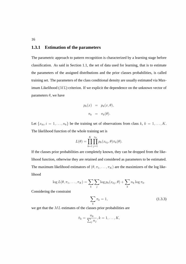
1.3.1 Estimation of the parameters
The parametric approach to pattern recognition is characterized by a learning stage before
classification. As said in Section 1.1, the set of data used for learning, that is to estimate
the parameters of the assigned distributions and the prior classes probabilities, is called
training set. The parameters of the class conditional density are usually estimated via Max-
imum Likelihood (ML) criterion. If we explicit the dependence on the unknown vector of
parametersθ, we have
pk(x) = pk(x, θ),
πk = πk(θ).
Let xki, i = 1, . . . , nk be the training set of observations from classk, k = 1, . . . , K.
The likelihood function of the whole training set is
L(θ) =K∏
k=1
nk∏j=1
pk(xkj, θ)πk(θ).
If the classes prior probabilities are completely known, they can be dropped from the like-
lihood function, otherwise they are retained and considered as parameters to be estimated.
The maximum likelihood estimators of(θ, π1, . . . , πK) are the maximizers of the log like-
lihood
log L(θ, π1, . . . , πK) =∑
k
∑j
log pk(xkj, θ) +∑
k
nk log πk.
Considering the constraint∑
k
πk = 1, (1.3.3)
we get that theML estimates of the classes prior probabilities are
πk =nk∑j nj
, k = 1, . . . , K,

17
that are the proportion of training samples from classk over the whole training set obser-
vations. The ML estimates of the remaining parameters are then obtained maximizing the
function
log L(θ) =∑
k
∑j
log pk(xkj, θ) + constant,
overθ. More often the parameters to be estimated divide into separate vectorsθk specific
for each classk, thus the ML estimators are obtained maximizing each class specific log
likelihood
log Lk(θk) =∑
j
log pk(xkj, θk) + constant, k = 1, . . . , K
over θk. As example if we assume that the class conditional pdf arep-variate normal
N(µk, Σk), the ML estimates of the mean vectorµk and of the variance matrixΣk are
given by their empirical analogs
µk =1
nk
nk∑i=1
xik,
Σk =1
nk
nk∑i=1
(xik − µk)(xik − µk)′ ,
for everyk = 1, . . . , K.
1.3.2 Linear discriminant analysis
Suppose the feature vector components are statistically independent with the same variance
σ2. In this simple case the covariance matrix is equal for each classk, k = 1, . . . , K and
diagonalΣk = Σ = Iσ2, whereI is the identity matrix. Observing that|Σ| = σ2p and
|Σ|−1 = I(1/σ2) and dropping the terms that are not class dependent, the (1.3.2) can be
rewritten as
gk(x) = −‖x− µk‖2
2σ2+ ln πk k = 1, . . . , K
18
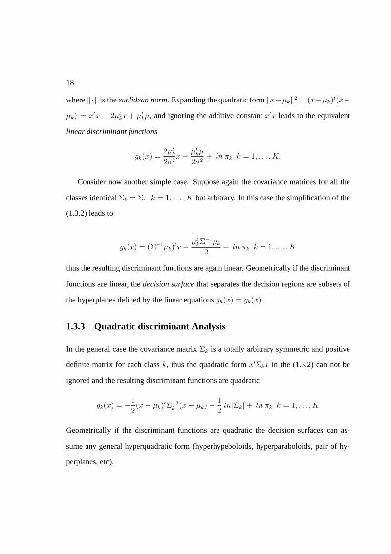
where‖·‖ is theeuclidean norm. Expanding the quadratic form‖x−µk‖2 = (x−µk)t(x−
µk) = xtx − 2µtkx + µt
kµ, and ignoring the additive constantxtx leads to the equivalent
linear discriminant functions
gk(x) =2µt
k
2σ2x− µt
kµ
2σ2+ ln πk k = 1, . . . , K.
Consider now another simple case. Suppose again the covariance matrices for all the
classes identicalΣk = Σ, k = 1, . . . , K but arbitrary. In this case the simplification of the
(1.3.2) leads to
gk(x) = (Σ−1µk)tx− µt
kΣ−1µk
2+ ln πk k = 1, . . . , K
thus the resulting discriminant functions are again linear. Geometrically if the discriminant
functions are linear, thedecision surfacethat separates the decision regions are subsets of
the hyperplanes defined by the linear equationsgh(x) = gk(x).
1.3.3 Quadratic discriminant Analysis
In the general case the covariance matrixΣk is a totally arbitrary symmetric and positive
definite matrix for each classk, thus the quadratic formxtΣkx in the (1.3.2) can not be
ignored and the resulting discriminant functions are quadratic
gk(x) = −1
2(x− µk)
tΣ−1k (x− µk)− 1
2ln|Σk|+ ln πk k = 1, . . . , K
Geometrically if the discriminant functions are quadratic the decision surfaces can as-
sume any general hyperquadratic form (hyperhypeboloids, hyperparaboloids, pair of hy-
perplanes, etc).

19
1.4 Non parametric discriminant analysis
The common parametric forms rarely fit the actual underlying class densities. When no
distribution assumptions within each class is made, nonparametric methods can be used
to estimate the class specific densitiespk(x), k = 1, . . . , K. Non parametric discrimi-
nant analysis (NPDA) consists in classification criteria based on nonparametric estimates
of class specific pdf. In NPDA, the class membership of each observedx can be evalu-
ated plugging in the Bayes classification rule the class specific densities estimated from
the training set and their prior probabilities. A popular non parametric estimation of the
density function is given by this is the case ofkernel methods.
In order to introduce the kernel approach, we start considering the univariate case. As-
sume we have a random samplex1, . . . , xn taken from a univariate continuous densityf .
The kernel density estimatorf of f is defined as
f(x, h) =1
nh
n∑i=1
K
(x−Xi)
h
, (1.4.1)
whereh is a positive number calledbandwidthor smoothingparameter andK is a function
calledkernelsatisfying ∫
RK(x)dx = 1 .
As we can see from equation (1.4.1), the kernel estimate at some pointx is the average
of then kernel centered at each observationxi and scaled byh. It can be shown that the
choice of the kernel function is not particularly important in the sense that the ”goodness”
of the estimation slightly depend on the shape ofK but it is strongly influenced by the
choice of the smoothing parameterh. In the classical parametric statistics the goodness
20
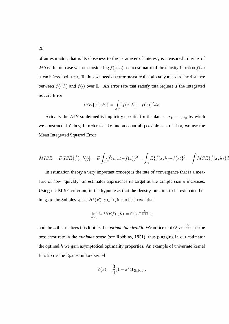
of an estimator, that is its closeness to the parameter of interest, is measured in terms of
MSE. In our case we are consideringf(x, h) as an estimator of the density functionf(x)
at each fixed pointx ∈ R, thus we need an error measure that globally measure the distance
between ˆf(·, h) andf(·) overR. An error rate that satisfy this request is the Integrated
Square Error
ISEf(·, h) =
∫
Rf(x, h)− f(x)2dx.
Actually theISE so defined is implicitly specific for the datasetx1, . . . , xn by witch
we constructedf thus, in order to take into account all possible sets of data, we use the
Mean Integrated Squared Error
MISE = E[ISEf(., h)] = E
∫
Rf(x, h)−f(x)2 =
∫
REf(x, h)−f(x)2 =
∫MSEf(x, h)dx.
In estimation theory a very important concept is the rate of convergence that is a mea-
sure of how ”quickly” an estimator approaches its target as the sample sizen increases.
Using the MISE criterion, in the hypothesis that the density function to be estimated be-
longs to the Sobolev spaceHs(R), s ∈ N, it can be shown that
infh>0
MISEf(·, h) = On− 2s2s+1,
and theh that realizes this limit is theoptimal bandwidth. We notice thatOn− 2s2s+1 is the
best error rate in theminimaxsense (see Robbins, 1951), thus plugging in our estimator
the optimalh we gain asymptotical optimality properties. An example of univariate kernel
function is the Epanechnikov kernel
K(x) =3
4(1− x2)1|x|<1.

21
Consider now the multivariate case. Ap-variate kernelK is a function fromRp to R
satisfying
∫K(x)dx = 1, x ∈ Rp
In the most general form, the p-dimensional kernel estimator is
f(x; H) =1
n
n∑i=1
KH(x− xi) (1.4.2)
whereH is a positive definite symmetric(p, p) matrix calledbandwidth matrixand its
elements are calledsmoothing parameters; furthermore
KH(x) = |H|−1/2K(H−1/2x).
As in the univariate case, (see Wand and Jones, 1995) if the density function to be estimated
belongs to the Sobolev spaceHs(Rp), s ∈ N, it can be shown that
infH∈Sp
MISEf(·, H) = On− 2s2s+p, (1.4.3)
whereSp is the set of symmetric and positive definite(p, p) matices. TheH that realizes
this limit is the optimal bandwidth matrix. We notice again thatOn− 2s2s+p is the best
error rate in theminimaxsense (see Robbins, 1951), thus again plugging in our estimator
the optimalH we gain an asymptotical optimality properties.
Unfortunately in the multivariate case the rate of convergence of any asymptotical op-
timal density estimator becomes slower as the dimensionp increases. This slower rate is
a manifestation of thecourse of dimensionalityor empty space phenomenon(Scott atal.,
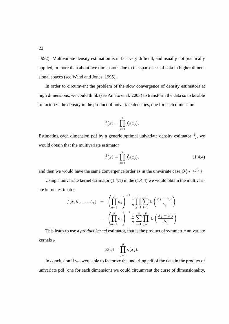
22
1992). Multivariate density estimation is in fact very difficult, and usually not practically
applied, in more than about five dimensions due to the sparseness of data in higher dimen-
sional spaces (see Wand and Jones, 1995).
In order to circumvent the problem of the slow convergence of density estimators at
high dimensions, we could think (see Amato et al. 2003) to transform the data so to be able
to factorize the density in the product of univariate densities, one for each dimension
f(x) =
p∏j=1
fj(xj).
Estimating each dimension pdf by a generic optimal univariate density estimatorfj, we
would obtain that the multivariate estimator
f(x) =
p∏j=1
fj(xj), (1.4.4)
and then we would have the same convergence order as in the univariate caseOn− 2s2s+1.
Using a univariate kernel estimator (1.4.1) in the (1.4.4) we would obtain the multivari-
ate kernel estimator
f(x, h1, . . . , hp) =
(p∏
d=1
hd
)−11
n
p∏j=1
n∑l=1
k
(xj − xlj
hj
)
=
(p∏
d=1
hd
)−11
n
n∑l=1
p∏j=1
k
(xj − xlj
hj
)
This leads to use aproduct kernelestimator, that is the product of symmetric univariate
kernelsκ
K(x) =
p∏j=1
κ(xj).
In conclusion if we were able to factorize the underling pdf of the data in the product of
univariate pdf (one for each dimension) we could circumvent the curse of dimensionality,

23
using for each univariate pdf an asymptotically optimal univariate density estimator. In
the next sections we will face the problem of finding a transformation of the original data
such that the transformed variables cumulative pdf could be estimated trough a product
kernel. The transformed variables should be the underlying factors or components that
describe the essential structure of the data. It is hoped that these components correspond to
some physical causes that were involved in the process that generated the data in the first
place. We will consider linear transformations only, because then the interpretation of the
representation is simpler, and so is its computation. Thus we will express the transformed
variables as a linear combination of the observed variables. In matrix representation we
have
y = Tx (1.4.5)
whereT is not necessarily a square matrix. In the following sections, we discuss some
statistical properties that could be used to determine the transformation matrixT .
In order to relate the multivariate kernel density estimation to our classification prob-
lem, we remember we want to estimate the probability density function of each classj,
using theNj observations from the training sample (j ∈ 1, . . . , K). The general form of
the classk (p-dimensional) kernel density estimator is
fk(x; Hk) =1
Nk
Nk∑i=1
KHk(x− xki) (1.4.6)
whereHk is the bandwidth matrix specific for classK, andxki, i = 1, . . . , Nk is the
training sample from the populationk. For a full discussion on the choice ofsmoothing
parameters, see Silverman, 1986.

24
Choosing a diagonal bandwidth matrix and the univariateκ as the normal density func-
tion leads to the class densities estimates
fk(x) = (2π)−p/2
(p∏
d=1
hkd
)−11
Nk
Nk∑l=1
p∏j=1
exp
−(xj − xlkj)
2
2h2kj
(1.4.7)
calledgaussian productkernel estimators. Equation (1.4.7) is very popular in multivariate
kernel density estimation.
1.4.1 Principal component discriminant analysis
One statistical principle for choosing the transformation matrixT in (1.4.5) is to limit the
number of componentsyi to be quite small so that they contain as much information on the
data as possible. This leads to a family of techniques called principal component analysis or
factor analysis. Given a vectorx of a large numberp of interrelated random variables, the
main idea ofprincipal components analysis(PCA) is to look for a fewer number (<< p)
of derived variables that retains the variation present in the component ofx as much as
possible. ThePCA procedure consists in transforming the original set of variables to the
principal components variables (PCs), which are uncorrelated and ordered so that most of
the original set variation is concentrated in the first few. The choice of the most important
PCs number is more or less an heuristic decision, and it may depend on the application.
We will briefly show the derivation ofPCA using the covariance method. We can interpret
PCA as a linear transformation that chooses a new coordinate system to represent the data
in order to have that by any projection of the data set, the greatest variance comes to lie
on the first axis (called the first principal component), the second greatest variance on the
second axis, and so on. Therefore, assumingx has zero empirical mean, we want to find an

25
orthonormal projection matrix P such that the transformed datay = P tx are uncorrelated.
This results in finding an orthogonal matrixP such thaty covariance matrixD is diagonal
D = cov(y) = diag(a1, . . . , ap)
whereai = var(yi), i = 1, . . . , p. It’s easy to see that
D = P tcov(x)P
and thus
PD = cov(x)P
Indicating each column ofP aspi, we get
aipi = cov(x)pi
This last expression reveals a simple way to calculate thePCs that consists in finding
the eigenvectors ofx covariance matrix. It turns out that the eigenvectors with the largest
eigenvalues correspond to the dimensions that have the strongest correlation in the data set.
The original measurements are finally projected onto the reduced vector space. Note that
the eigenvectors ofcov(x) are actually the columns of the matrix V, where cov(x)=ULV’ is
the singular value decomposition (SV D) of cov(x). For a detailed description ofPCA see
Jolliffe, 2002.
PCA is a popular technique in pattern recognition and we will use it only to linearly trans-
form the data in order to decorrelate them before the classification step. In practice, the
training data from each classk are used to compute the sample mean and the sample co-
variance matrix of the centered data from classk. The projection matrixPk for each class
k is then evaluated viaSV D procedure. Using theNk observation from classk training
26
set,the transformed dataylk = P tkxlk are calculated and so for each classk and for each di-
mensionj, the univariate pdfgkj of the transformed variableyk j-th component is estimated
via univariate kernel density estimator. The resulting product kernel density estimator for
yk is gk(yk) =∏p
j=1 gkj(ykj). A change of variablesx = Pky allows to go back to the
original data domain and get the estimation of the classk pdf
fk(x) = gk(Ptkx)|det(Pk)| =
p∏j=1
gkj((Ptkx)j). (1.4.8)
However,PCA just decorrelates the data without making them independent. Thus the
factorization in (1.4.10) can be supported only under the assumption of independence that
is not valid unless the data are Gaussian. In fact if we assume that classk pdf is a p-
variate normalNp(µk, Σk) of meanµk and covarianceΣk, then the random vectory = P tkx
has ap-variate normal pdfNp(Ptkµk, Dk) with covariance matrixDk diagonal and so has
independent components, thus in this case the factorization in (1.4.10) holds because for
gaussian data uncorrelated components are always independent.
1.4.2 Independent components discriminant analysis
Another principle that has been used for determining the matrixT in (1.4.5) is indepen-
dence: the componentsyi should be statistically independent. This means that the value of
any one of the components gives no information on the values of the other components. As
seen in the previous Section, inPCA the transformed variables are assumed to be indepen-
dent, but this is only true when the data are assumed to be gaussian. In reality, however, the
data often do not follow a gaussian distribution. Independent Component Analysis (ICA)
is a statistical method whose main target is to find statistically independent components, in
27
the general case where the data are non gaussian. We could define ICA as a linear trans-
formation given by a matrix as in (1.4.5), so that the transformed random variables are
as independent as possible. A very intuitive and important principle of ICA estimation is
maximum non gaussianity. The idea is that according to the central limit theorem, sums of
non gaussian independent random variables are closer to gaussian than the original ones.
Therefore, if we take a linear combination of the observed variables, this will be maximally
non gaussian if it equals one of the independent components. This is because according to
the central limit theorem, if it was a real mixture of two or more components, it would be
closer to a gaussian distribution.
A very important measure of non gaussianity is given by negentropy. Negentropy is
based on the differential entropy. The differential entropyH of a random vectory with
densityf(y) is defined asH(y) = − ∫f(y)logf(y)dy, (Cover and Thomas, 1991). Ne-
gentropyJ is defined asJ(y) = H(ygauss) − H(y), whereygauss is a Gaussian random
variable of the same covariance matrix asy. The estimation of negentropy is difficult and
in practice, some approximation have to be used. Here we introduce the approximation
proposed by Hyvarinen (1997) that has very promising properties, and which will be used
in the following to derive an efficient method for ICA. Hyvarinen approximates the negen-
tropyJ(y) as
JG(y) =
p∑i=1
E(G(yi)− E(G(Z))2 (1.4.9)
whereZ is a zero-mean standard normal random variable and the functionG, called con-
trast function, is usually the power three transform. We refer to Hyvarinen(1997) for the
details of the derivation of theICA transformy = Tx and of its statistical properties.
ICA is can be used in pattern recognition to linearly transform the data in order to
28
make them approximately independent before the classification step. This approach was
first introduced by Amatoet al (2003). In practice, the training data from each classk
are used to compute the sample mean and the centered data are then used to derive the
ICA transformation matrixTk for classk sample. Using theNk observations from class
k training set,the transformed dataylk = Tkxlk are calculated and so for each classk and
for each dimensionj, the univariate pdfgkj of the transformed variableyk j-th component
is estimated via univariate kernel density estimator. The resulting product kernel density
estimator foryk is gk(yk) =∏p
j=1 gkj(ykj). A change of variablesx = T−1k y allows to go
back to the original data domain and get the estimation of the classk pdf
fk(x) = gk(Akx)|det(Ak)| =p∏
j=1
gkj((Tkx)j)|det(Ak)| (1.4.10)
whereAk is the pseudo inverse ofTk. Amato et al. (2003) showed that the decision
rule resulting substituting the estimated class pdffk in the 1.2.6 converges uniformly in
probability to the Bayes classification rule and is asymptotically optimal.
1.5 Local Discriminant methods for image classification
In the present and following sections we shall deal with supervised classification of bidi-
mensional images. The general problem can be formulated as follows. A continuous two
dimensional region is partitioned into a finite number of sites called pixels (pictures ele-
ments), each pixel belonging to one of a predefined finite set of classes1, . . . , K. The
set can represent, e.g., land cover categories, cloudy or clear sky conditions, etc.. The true
labelling of the region is unknown but associated with each pixel there is a multivariate
(actually, multispectral) value which provides information about its label. Bayesian dis-
criminant analysis consists in choosing the classk from the set1, . . . , K according to
29
the Bayes decision rule (1.2.6). Several discriminant analysis methods have been proposed
in the literature, according to the choice of the class conditional densitiespk(x) parametri-
cally (e.g., Gaussian) or nonparametrically (e.g., Kernel density estimation) and to the way
the multidimensionality ofx is faced. It is out of the scope of the present chapter to review
the methods developed in the framework of discriminant analysis. Rather, we shall focus
on the observation that traditional image classification approaches often neglect the infor-
mation about spatial relationships between adjacent pixels. In other words, classification
through Eq. (1.2.6) is performed pixel-wise and no information on other pixels, neither
the surrounding ones, is used. However, pixels belonging to a same class tend often to
cluster together in many applications, and remote sensing is just one of these. Referring to
the above mentioned examples, land cover and cloud fields usually extend over regions of
several pixels, depending on the spatial resolution of the sensor. Also note that strict appli-
cation of Bayes decision rule gives rise to typical ‘pseudo-noisy’ reconstructed label fields,
where often isolated labels are present that are not physically feasible (that is, a pixel be-
longs to a certain class, and all surrounding pixels belong to other, different classes). This
effect is disturbing especially in the analysis of medical images, where sometimes these
isolated pixels refer to tissues that cannot be present in the corresponding locations. This
effect is intrinsic to the discriminant analysis and is due to the uncertainty of the decision
rule coming from the overlap of the probability density functions among different classes:
the more such density functions are overlapped, the bigger the effect of ‘pseudo-noise’.
To overcome this problem, the procedure usually used is an empirical post-processing of
the retrieved label field, where a sort of smoothing of the label field obtained by discrimi-
nant analysis is accomplished in a remote sensing application (see Ju, Gopal,and Kolaczyk,
30
2005).
An attempt to incorporate pixel context in image classification goes back to the Iterated
Conditional Modes (ICM) (Besag, 1986). Basically, this method assumes that the true
label set of an image is a realization of a locally dependent Markov Random field so that
the posterior class probability for a specific data point also depends on the labelling of
its neighborhood. After obtaining a first class estimate for each pixel using any non local
method, local (i.e., depending on the location in the image) priori probabilities of classes
are computed from the estimate, considering a neighbor of each pixel; then new labels are
assigned to the pixels maximizing the class posterior probability and relying on the prior
probabilities just estimated. The procedure is iterated until convergence. ICM method
has been applied successfully in the field of remote sensing (Khedam et al., 2004) and
compared to Maximum Likelihood classification (Keuchel et al., 2003).
In the following we first formalize discriminant analysis in a framework that focuses
on how much a class can be visible or nonvisible, then we introduce some discriminant
analysis methods that use spatial information around each pixel in order to localize the
methods. We have the twofold objective of a) improving local label estimates by increasing
the number of pixels (i.e., information) involved in the decision rule; b) reducing of the
‘pseudo-nuisance’ present in pixel-wise discriminant analysis. These methods will be best
suited for visible and nonvisible classes. Numerical experiments will be performed. In
particular, methods will be applied to the problem of retrieving cloud mask from remote
sensed images.
31
1.6 Notations and Assumptions
Let us consider a general case where an object has to be classified as coming from one of
a fixed number of predefined classes, say1, . . . , K. Associated with this object there is
possibly a multivariate recordx = (x1, . . . , xD) belonging to a subsetχ of RD and it is
interpreted as a particular realization of a random vectorX = (X1, . . . , XD). In our case,
without any loss of generality, an object is a pixel of an image and it is usually identified
by a couple of coordinates. With a slight abuse of notation, we will identify an observation
or pixel with its measurementx when no ambiguity arises.
In the present work we shall consider the univariate case. This does not restrict applica-
bility of the methods we are going to consider, since extension to theD-dimensional case
is straightforward. In addition this assumption is particularly suited for those applications
where only univariate measurements (D = 1) are available, or one covariate is already able
to give good classification rates with respect to the multivariate case; then improvement
of the univariate classification could give classification rates comparable with those of the
(more expensive) multivariate case.
Let us now consider first the case where the random variableX is discrete, soχ = 1, . . . , N ⊆N.
For the purpose of the present paper, we introduce the following definitions.
Definition1. x ∈ χ is calleddominant for the class k with respect to a Bayes classificationruleγ if and only if p(k|x) ≥ p(i|x), i = 1, . . . , K.
Definition2. Fork = 1, . . . , K we definedominant set,Dγk , for classk with respect to the
Bayes ruleγ, the set
Dγk := x ∈ χ : x is dominant for the class k and the rule γ.
32
Definition3. For k = 1, . . . , K we definedominance indexof classk with respect to theBayes classification ruleγ, δγ(k), the quantity
δγ(k) :=∑
x∈Dγk
pk(x), k = 1, . . . , K.
Definition 3 assumes that a dominant yields only one classk. In the general case this is
not the rule; then let us give the following
Definition4. A target class of an observationx ∈ χ, κ(x), with respect to the Bayes ruleγis the set of classes for whichx is dominant:
κ(x) := k : x is dominant for k, 1 ≤ k ≤ K.
Let
wk(x) =1
|κ(x)| ,
with | · | being cardinality of the set. Then Definition 3 can be generalized as
δγ(k) :=∑x∈Dk
wk(x)pk(x), k = 1, . . . , K
that for eachx ∈ χ corresponds to assign equal probability of occurrence to all classes
for whichx is dominant. In the following we assume for simplicity’s sake that a dominant
yields only one class, so thatw(k) = 1.
The above formalism can be applied to probability density functions provided that Def-
inition 3 is changed as
Definition5. Fork = 1, . . . , K we definedominance indexof classk, δγ(k), with respectto the Bayes classification ruleγ, the quantity
δγ(k) :=
∫
Dγk
pk(x)dx, k = 1, . . . , K.
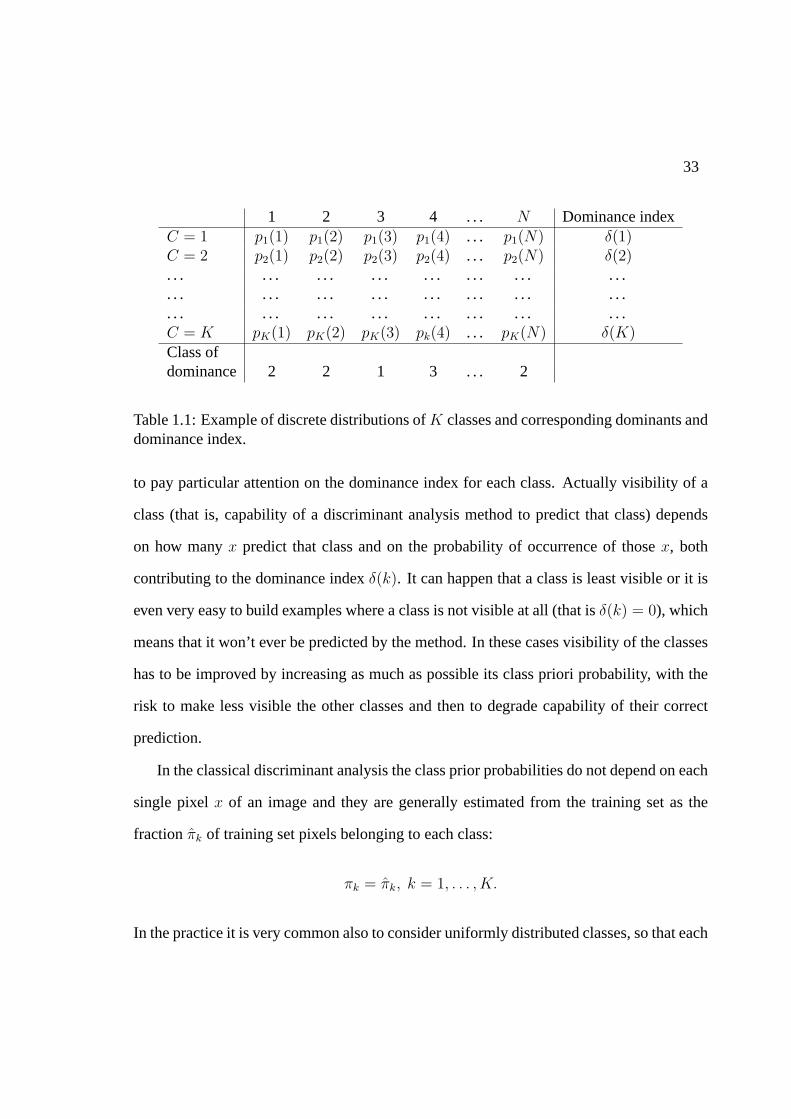
Table 1.1 shows an example of discrete probabilities with corresponding dominance
index and class of dominance supposing, e.g., constant priori class probabilities. We want
33
1 2 3 4 . . . N Dominance indexC = 1 p1(1) p1(2) p1(3) p1(4) . . . p1(N) δ(1)C = 2 p2(1) p2(2) p2(3) p2(4) . . . p2(N) δ(2). . . . . . . . . . . . . . . . . . . . . . . .. . . . . . . . . . . . . . . . . . . . . . . .. . . . . . . . . . . . . . . . . . . . . . . .C = K pK(1) pK(2) pK(3) pk(4) . . . pK(N) δ(K)Class ofdominance 2 2 1 3 . . . 2
Table 1.1: Example of discrete distributions ofK classes and corresponding dominants anddominance index.
to pay particular attention on the dominance index for each class. Actually visibility of a
class (that is, capability of a discriminant analysis method to predict that class) depends
on how manyx predict that class and on the probability of occurrence of thosex, both
contributing to the dominance indexδ(k). It can happen that a class is least visible or it is
even very easy to build examples where a class is not visible at all (that isδ(k) = 0), which
means that it won’t ever be predicted by the method. In these cases visibility of the classes
has to be improved by increasing as much as possible its class priori probability, with the
risk to make less visible the other classes and then to degrade capability of their correct
prediction.
In the classical discriminant analysis the class prior probabilities do not depend on each
single pixelx of an image and they are generally estimated from the training set as the
fractionπk of training set pixels belonging to each class:
πk = πk, k = 1, . . . , K.
In the practice it is very common also to consider uniformly distributed classes, so that each

34
class has the same prior probability:
πk =1
K, k = 1, . . . , K.
These assumptions give rise tonaıveclassification rules,γnaıve, that globally take best ac-
count of the occurrence probability of the classes or do not privilege the classes a priori at
all.
1.7 Local priors
Nonlocal priors of Section 1.6 take account of the global occurrence of the classes over an
image and do not take any account of spatial correlation or of local features in an image.
In particular when an image has a wide homogeneous region labelled by the same classk,
the spatial correlation is maximum and it appears natural to be more confident about the
presence of classk in pixels belonging to that region. Note that this is the rule in most
applications of image classification. Moreover, location of these homogeneous regions
cannot be predicted in advance in several applications, especially when different images
have to be classified. In particular we cannot rely in general on the training images to this
purpose, nor we can assume that the naıve global priors represent the true local probability
of occurrence of classes accurately. For these reasons local priors are prone to improve
accuracy of classification in homogeneous regions, provided that a good estimation of prior
classes probabilities can be given.
In this Section we propose some methods that exploit information contained in the
neighborhood of each single pixel; they modify the posterior probability estimates given
by Eq. (1.2.3) introducing a set of local prior probabilities,πk(x)k=1,...,K , specific for
35
each single pixelx of an image:
p(k|x) = Pr(C = k|X = x) =πk(x)pk(x)∑Ki=1 πi(x)pi(x)
. (1.7.1)
Let us consider for each pixelxc a neighborhood regionB(xc). This region can have any
shape and size. Furthermore let
Bk(xc) := x ∈ B(xc) : γ(x) = k
be the set of pixels labelled ask in the neighborhoodB(xc). Let us indicate asL(B(xc); γ)
the set of labels associated to all pixels of an image by any discriminant ruleγ.
In the following sections we introduce some classification Bayes-like rules relying on
Eqs. (1.7.1) and (1.2.6), differing in the way of estimating class prior local probabilities.
1.7.1 Local voting priors
Suppose an estimate of class label is available for all pixels through a classical Bayes rule
(1.2.6) with some a priori class probabilities. Let
ϕk(xc) =|Bk(xc)||B(xc)| , k = 1, . . . , K, (1.7.2)
be the relative frequency of labelsk in B(xc). Intuitively , for any pixelxc, we would
estimate the set of prior probabilitiesπk(xc)k=1,...,K in order to enhance the class with
the highest relative frequency inB(xc). Thus a first attempt to estimate the generic classk
prior probabilityπk(xc) is :
πLVk (xc) =
1 if k = argmaxj=1,...,Kϕj(xc),0 otherwise.
(1.7.3)
36
The local priors just defined naturally satisfy the constraint (1.3.3). By using initial (first-
guess) a priori class probabilities and by an iterative application of the above mentioned
procedure until convergence, we obtain final class prior probabilities and corresponding
class labels. We call these priorsLocal Voting priors. The arising classification method is
well suited for those classes that are visible, since it is able to maximize their visibility.
1.7.2 Local frequency priors
Under the same hypothesis of the previous subsection, we propose now to estimate the
classk prior probabilityπk(xc) by the relative frequency ofk labels inB(xc):
πLFk (xc) = ϕk(xc), k = 1, . . . , K.
They naturally satisfy the constraint (1.3.3). As with Local Voting priors, the procedure is
iterated until convergence thus obtaining the final class prior probabilities and correspond-
ing class labels. We call these priorsLocal Frequency priors. Since priors are based on
the relative occurrence frequencies resulting from some discriminant analysis method,ϕk,
then the resulting classification method is again well suited for those classes that are visi-
ble, since it is able to enhance their visibility, but does not penalize the less visible classes
as much as the Local Voting method.
1.7.3 Local integrated priors
Given a pixelxc and its neighborB(xc) we estimate the prior probabilityπk(xc) for the
generic classk by summing the probability density functionspk(x) over the neighborhood
regionB(xc):
πLIk (xc) ∝
∑
x∈B(xc)
pk(x), k = 1, . . . , K.

37
We define these priorsLocal Integrated priors. If we consider the normalization
πLIk (xc) =
∑x∈B(xc)
pk(x)∑K
j=1
∑x∈B(xc)
pj(x), k = 1, . . . , K, (1.7.4)
then the set of local priorsπLIk (xc) satisfies constraint (1.3.3). Each data point label is then
estimated through Eq. (1.7.1) using the local class prior probabilities (1.7.4). Notice that
this method is not iterative. Moreover these priors are not related to the class prediction ob-
tained by some discriminant analysis method, so that they naturally tend to be not sensitive
to visibility or nonvisibility of a class; in practice they are suited for nonvisible classes.
1.7.4 Local nested priors
Suppose again, as in subsections (1.7.1) and (1.7.2), that a first-guess estimate of each
data point label is obtained by the classical Bayes rule (1.2.6) with some a priori class
probabilities. Given a pixelxc and its neighborB(xc), we estimate the prior probability
πk(xc) for the generic classk by summing its posterior probabilityp(k|x) over the region
B(xc):
πLNk (xc) ∝
∑
x∈B(xc)
p(k|x), k = 1, . . . , K.
To satisfy the constraint (1.3.3), priorsπLNk are normalized as
πLNk (xc) =
1
|B(xc)|∑
x∈B(xc)
p(k|x), k = 1, . . . , K. (1.7.5)
The procedure is iterated until convergence. We define these priorsLocal Nested priors.
As far as visibility of classes is concerned, these priors are a sort of trade-off between
LF (suited for visible classes) and LI (suited for nonvisible classes), since they depend on
the class label of some discriminant analysis method, but anyway potentially include the
contribution of probability density functions all over their domain.

38
1.8 Asymptotics
We now discuss asymptotic behavior of the local priors considered in Section 1.7. To this
purpose let the neighborhood regionB(xc) of each pixelxc tend to infinity and assume that
B(xc) is a homogeneous region of class`, 1 ≤ ` ≤ K.
1.8.1 Local voting priors
Let’s consider the asymptotic behavior of the local frequency priors[πLVk ], k = 1, . . . , K,
defined in section (1.7.1). Even if the classification process they generate is iterative and
local, the dependence from the iteration is lost asimptotically. In fact if we let the neigh-
borhood region of the generic pixel tend to infinity we get that the local voting prior for the
generic class k behaves as
πLVk = δ(k, k) =
1 if k = k,
0 otherwise,
where
k = argmaxk=1,...,K
P (x ∈ Dk | C = `). (1.8.1)
We point out thatDk is the dominant set defined in (2) at the first step of the iterative
process described in subsection 1.7.1. More explicitly in (1.8.1) we have
P (x ∈ [Dk] | C = `) =∑x∈Dk
p`(x), k = 1, . . . , K
in the discrete case, and
P (x ∈ [Dk] | C = `) =
∫
x∈Dk
p`(x), k = 1, . . . , K
in the continuous case.

39
1.8.2 Local frequency priors
It is easy to see that at each iterationν, the local frequency priors[πLFk ]ν , k = 1, . . . , K,
asymptotically behave as the probabilityP (x ∈ [Dk]ν−1 | C = `), where[Dk]
ν−1 is the
dominant set at the stepν − 1 of the iterative process described in subsection 1.7.2. It
follows
[πLFk ]ν →
∑
x∈[Dk]ν−1
p`(x), k = 1, . . . , K
in the discrete case, and
[πLFk ]ν →
∫
x∈[Dk]ν−1
p`(x), k = 1, . . . , K
in the continuous case.
1.8.3 Local integrated priors
Equation (1.7.4) can be rewritten as
πLIk (xc) =
∑x∈B(xc)
pk(x)
|B(xc)|1
∑Kj=1
∑x∈B(xc) pj(x)
|B(xc)|
, k = 1, . . . , K,
so that we can say
πLIk (xc) ∝
∑x∈B(xc)
pk(x)
|B(xc)| , k = 1, . . . , K. (1.8.2)
Equation (1.8.2) tells us that asymptotically the local integrated priors tend to be propor-
tional to∑x∈χ
pk(x)p`(x), k = 1, . . . , K.
in the discrete case, and to∫
χ
pk(x)p`(x)dx, k = 1, . . . , K.
in the continuous case.

40
1.8.4 Local nested priors
Consider iterationν of the iterative process described in the Section 1.7.4. From Eq. (1.7.5)
it follows that asymptotically the local nested priors [πLNk ]ν , k = 1, . . . , K, tend to
∑x∈χ
pν−1(k|x)p`(x)dx, k = 1, . . . , K (1.8.3)
in the discrete case, and to∫
χ
pν−1(k|x)p`(x)dx, k = 1, . . . , K (1.8.4)
in the continuous case. More explicitly Eq. (1.8.3) can be rewritten as
[πk]ν−1
∑x∈χ
pk(x)p`(x)∑Kj=1[πj]ν−1pj(x)
, k = 1, . . . , K
and Eq. (1.8.4) as
[πk]ν−1
∫
χ
pk(x)p`(x)∑Kj=1[πj]ν−1pj(x)
dx, k = 1, . . . , K
1.8.5 Iterations
In LF and NF methods priori class probabilities are defined in terms of an iterative proce-
dure. Therefore the natural question arises about the presence of more solutions. It is easy
to see that both methods surely admits several solutions. In particular we can see that, e.g.,
(1, 0, 0, . . . , 0), (0, 1, 0, . . . , 0), . . ., (0, 0, 0, . . . , 1) are all solutions (that we calltrivial ) of
the local classification methods. These solutions are obtained starting iterations with the
same final values. In the general case we found that final solutions are very robust with
respect to the first-guess chosen and that a few iterations are sufficient to get convergence.
As a practical rule it is possible to start from constant class priori probabilities over the
classes.
Chapter 2
Multiple Hypothesis Testing
Introduction
In this chapter we introduce the statistical problem of multiple hypothesis testing and re-
view the guiding lines of frequentist and Bayesian approach to it, describing strength and
weakness of the two philosophies and trying to find some connections between them. We
describe a specific multiple hypothesis testing problem, and propose a new testing pro-
cedure that represents a sort of ”empirical” approach. The application of the described
methods to a genetic microarray data experiment is provided in Chapter 6.
The Chapter is organized as follows. The first section is a brief overview of the multiple
hypothesis testing (MHT ) problem. In Section 2 some recent error measures forMHT
are introduced and multiple testing error controlling procedures (MTP ) are described in
Section 3. In Section 4 bootstrap methods are presented.MHT in the Bayesian framework
is introduced in Section 5. In Section 6, MAP multiple testing procedure is described and
a newMHT procedure is proposed.
41
42
2.1 General Framework
In the general framework of single hypothesis testing, we want to test the hypothesisH0
that an unknown parameterθ of a certain distribution belongs to some subspaceΘ0 ∈Rq (q ∈ N), against the alternative hypothesisH1 that θ belongs toΘ1 ⊆ Rq, where
Θ0
⋂Θ1 = ∅ . The solution of this problem is in terms of a rejection regionRt which
is a set of values in the sample space which leads to the decision of rejecting the null
hypothesisH0 in favor of the alternativeH1. Usually an hypothesis is formulated in order
to be rejected, so that we interpret a rejection as a discovery or positive result. In general
the rejection regionRt is constructed in order to control at some levelα the size of Type I
error, i.e. the probability of rejecting the null hypothesis when it is true, while looking for
a procedure that possibly minimize the probability of observing a false negative, i.e. the
Type II error. A standard approach is to specify an acceptable levelα for the Type I error
rate and derive testing procedures, i.e., rejection region, that aims to minimize the Type II
error rate, i.e., maximize the power, within the class of tests with Type I error rate at most
α. For single hypothesis testing, optimality results are available for particular types of data
generating distributions, null and alternative hypotheses, and test statistics. In a multiple
testing context we need a generalization of Type I and Type II error. Simultaneous testing of
multiple hypotheses has always attracted the attention of statisticians. Folks (1984) gives a
first introduction to multiple hypothesis testing. When thousands of hypotheses need to be
tested simultaneously, the traditional methods are not sensible because of loss of specificity
and power. To illustrate the problem, consider the gene expression example. Assume that a
chip reveals the expression level ofm = 10.000 genes relatively to two different biological
conditions and we know that not a single gene is differentially expressed. We want to

43
test, simultaneously for each gene, the null hypothesis that the gene is not differentially
expressed against the alternative that it is. If we test each of them hypothesis at level
α = 0.01, we would expect100 of the tests would havep-value less thenα ( i.e. we expect
about100 false positive) and the probability that al least onep-value is less thanα is about 1.
To illustrate the general procedure, consider the problem of testing simultaneouslym null
hypotheses. Suppose we havem independent vectors of observationsXj, j = 1, . . . , m,
of sizenj and the distribution of eachXj, fj(Xj | θj) , depends on a vector of parameters
θj ∈ Ωj ⊆ Rdj . Without loss of generality assumenj = n, j = 1, . . . , m. Usually in the
applicationsn is much smaller thanm. We want to test simultaneously each of them non
nested hypotheses
H0j = θj ∈ Θ0j vs H1j = θj ∈ Θ1j j = 1, . . . ,m, Θ0j ∪Θ1j = Ωj, Θ0j ∩Θ1j = ∅.(2.1.1)
This general representation covers tests of means, differences in means, parameters in
linear models, generalized linear models, and so on.
The decisions to reject or not the null hypotheses are based on test statistics, i.e., func-
tions of the data,Tj = T (Xj1, . . . , Xjn). The testing procedure provides rejection regions,
Rtj, i.e., sets of values for the test statisticsTj that lead to the decisions to reject the null
hypothesesH0j if Tj ∈ Rtj. Suppose thatm0 null hypotheses are true andR is the number
of hypotheses rejected. LetU andV be the numbers of the true null hypotheses respec-
tively accepted and rejected and letT andS be the numbers of the non true null hypothesis
respectively accepted and refused. This situation is summarized in Table 2.1.
While R is an observable random variable,U, V, S andT are not.
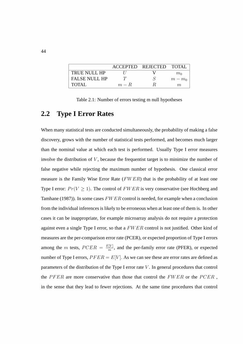
44
ACCEPTED REJECTED TOTALTRUE NULL HP U V m0
FALSE NULL HP T S m−m0
TOTAL m−R R m
Table 2.1: Number of errors testing m null hypotheses
2.2 Type I Error Rates
When many statistical tests are conducted simultaneously, the probability of making a false
discovery, grows with the number of statistical tests performed, and becomes much larger
than the nominal value at which each test is performed. Usually Type I error measures
involve the distribution ofV , because the frequentist target is to minimize the number of
false negative while rejecting the maximum number of hypothesis. One classical error
measure is the Family Wise Error Rate (FWER) that is the probability of at least one
Type I error:Pr(V ≥ 1). The control ofFWER is very conservative (see Hochberg and
Tamhane (1987)). In some casesFWER control is needed, for example when a conclusion
from the individual inferences is likely to be erroneous when at least one of them is. In other
cases it can be inappropriate, for example microarray analysis do not require a protection
against even a single Type I error, so that aFWER control is not justified. Other kind of
measures are the per-comparison error rate (PCER), or expected proportion of Type I errors
among them tests,PCER = E[V ]m
, and the per-family error rate (PFER), or expected
number of Type I errors,PFER = E[V ]. As we can see these are error rates are defined as
parameters of the distribution of the Type I error rateV . In general procedures that control
the PFER are more conservative than those that control theFWER or the PCER ,
in the sense that they lead to fewer rejections. At the same time procedures that control

45
theFWER are more conservative than those that control thePCER. Actually it can be
easily shown thatPCER ≤ FWER ≤ PFER (the order is reversed with respect to the
number of rejections). Benjamini and Hockberg (1995) suggested that in many multiplicity
problems the number of erroneous rejections should be taken into account and not only
the question wether any error was made. From this point of view they proposed, as new
error measure, the expected proportion of errors among the rejected hypotheses: the False
Discovery Rate (FDR). The proportion of null hypotheses that are erroneously rejected,
among all the rejected hypotheses, is a random variableQ that express the proportion of
errors committed by falsely rejecting null hypotheses. WhenR = V + S = 0, the random
variableQ should be set to zero as no error of false rejection can be committed. Therefore
if we define the False Discovery Proportion (FDP ) as
FDP =
Q = VR
if R > 0,
0 if R = 0
theFDR can be defined as the expected value ofQ:
FDR = E(FDP ) = E
(V
R|R > 0
)Pr(R > 0). (2.2.1)
FDR has become a popular tool for controlling the error in microarray analysis. In fact
the purpose of this kind of analysis is to individuate genes that are potential candidate for
further investigation. Thus few erroneous rejections will not distort the conclusions at this
stage of the analysis, as long as their proportion is small.
Note that the control ofFDR is implicitly a control ofFWER when all the null hypothesis
are true, in fact when all the null hypotheses are truem = m0, V = R, FDP = 1 and
consequentlyFWER = Pr(V ≥ 1) = Pr(R > 0) = FDR. The other way round, it’s
easy to see that whenm0 < m any procedure that controls theFWER also controls the

46
FDR. As we will see the controls of Type I error whenm = m0 andm0 < m are referred
to asweakandstrongcontrol. Storey (2001) suggested to control another quantity called
Positive False Discovery Rate (pFDR)
pFDR = E
(V
R|R > 0
). (2.2.2)
The termpositivedescribes the fact that we have conditioned on at least one positive
finding having occurred. We argue that whenm0 = m, one would want the false discovery
rate to be 1, and that one is not interested in cases where no test is significant. These
considerations lead Storey to propose definition (2.2.2) as an error rate alternative to (2.2.1).
In Storey (2003) thepFDR is used to define theq-value, which is a natural Bayesian
version of thepFDR analogue to thep-value.
2.2.1 Strong and Weak control
It is important to note that the error rates described above depend upon which specific
subset of null hypotheses is true for the (unknown) data generating distribution. A very
important distinction is that between strong and weak control of Type I error rate. This
distinction is pointed out in Westfal and Young (1993). Strong control relates to the control
of Type I error under any combination of true and false hypotheses. Weak control relates to
control of the Type I error rate when all the null hypotheses are true. Note that the concept
of strong and weak control applies to any of the Type I error rated defined above.

47
2.3 Error Controlling Procedures
Considerm independent statisticsT1, T2, . . . , Tm for the null hypothesesH01, H02, . . . , H0m.
We define thej-th p-value to be
pj = Pr(|Tj| > |tj| | H0j is true), j = 1, . . . , m
wheretj is the observed value of the test statisticTj. It is well known that eachp-value is
a random variable uniformly distributed in[0, 1] under any simple null hypothesis. Gen-
ovese and Wesserman (2002) define a marginal distribution for thep-values when the null
hypotheses are composite. We will deal only with the case of simple null hypotheses.
A multiple testing procedure (MTP ) aims to produce a set of rejected hypothesisRt(T1, ..., Tm, α) =
j ∈ 1, . . . , m : H0j is rejected to estimate the set of the false null hypothesis. The
setRt will depend on the data through the test statisticsTj and on the levelα fixed as up-
per bound for a suitably defined Type I error measure. In this dissertation the dependence
on the data will be carried out through thep-values. Usually each single hypothesisj is
rejected ifpj ≤ Tr whereTr is a data dependent critical value (cut-off) value, and the dif-
ferentMTP techniques specify a way to determine a well set cut off value. Some authors,
see as example Dudoitet al. (2003), prefer instead to define a new kind ofp-values, called
adjustedp-values, that are function of the classical concept ofp-value, and leave the cut
off fixed to a certainα. It can be shown that consider an adjustment of the critical value is
equivalent to consider an adjustment of thep-value for any givenMTP .
TheMTP are categorized as single-step procedures and stepwise procedures. In the single
step approach thep-values are compared to a predetermined cut off level that is a function
of the levelα and of the number of hypothesesm. As for the stepwise procedures, there

48
are two different approaches: the step-down and the step-up. The step-down (Holm, 1979)
starts with the most significant hypothesis and, as soon as one fails to reject a null hypoth-
esis, no further rejections are made. The step-up procedure (Hochberg, 1988) starts with
the least significant hypotheses and, as soon as one rejects a null hypothesis, rejects all
the hypotheses that are more significant. More explicitly, consider the orderedp-values:
p(1), . . . , p(m). The step-down procedures start examiningp(1) and continue rejecting until
the first acceptance, while the step-up procedures starts withp(m) and continue accepting
until the first rejection. It follows that the step-down procedures are more conservative than
the step-up
2.3.1 FWER and FDR Controlling Procedures
The most classical example ofFWER controlling procedure is the Bonferroni correction
which is a single-step procedure fixing a universal critical valueTr = αm
. This means that
one would reject only the hypotheses for which the correspondentp-value is less thanαm
.
OtherFWER controls are the one-step and the step-down proposed in Sidak (1967 and
1971), the step-down Holm (Holm, 1979), the step-up in Hochberg and Benjamini (1990),
and the step-downminP (Van der Laanet al., 2003).
The FDR defined in (2.2.1) is an error measure that provides less strict control on the
number of false positives so that theFDR controlling procedures has a gain in power with
respect to theFWER ones. The Benjamini-Hochberg (BH) is the most classicalFDR
controlling procedure, it consists in a step-up procedure that can be defined as follows:
reject all H0(i) s.t. i ≤ k = argmaxj=1,...,m
p(j) ≤ j
mq
wherep(1), . . . , p(m) are the orderedp-values,H0(i) is the null hypothesis corresponding
49
to p(i) andq is the chosenFDR upper bound. Benjamini and Hochberg (1995) showed that
the above procedure controlsFDR at levelq. Benjamini and Yekutieli (2001) proved that
theBH procedure controlsFDR at levelm0
mq when the number of true null hypothesesm0
is smaller thanm and the test statistics are continuous. Consequently if we knewm0, the
BH procedure could be improved by using as controlling levelq′ = mm0
q. In practicem0 is
unknown and many adaptive procedures which estimate this factor have been constructed;
see Efron et al. (2001), Storey (2002) and Benjamini and Yekutieli (2003) for a complete
review.
2.4 Bootstrap estimation of the null distribution
In principle we may make parametric assumption on the joint distribution of the test statis-
tics but these assumptions would seldom be reliable. In many practical situations the joint
and marginal distributions of the test statistics are unknown and so the true joint distribu-
tion G, for the test statisticsTj, j = 1, . . . , m, is estimated by a null joint distributionG0 in
order to derive the resultingp-values. The choice of a joint null distributionG0 is crucial to
ensure that the control of the Type I error rate actually provides the required control under
the true distributionG. Resampling methods such as bootstrap and permutation are used to
estimateG0. The name bootstrap alludes to pulling yourself up by your own boot strap. In
statistics Bootstrapping is a method for estimating the sampling distribution of interest by
resampling with replacement from the original sample of data. This means that one avail-
able sample gives rise to many others by resampling. Bootstrap technique was invented by
Bradley Efron (1979) and further developed by Efron and Tibshirani (1993). We describe
in the followings a generic bootstrap estimation procedure of the null distribution . The

50
first step is to generate B bootstrap samples starting from the data. Then for each bootstrap
sample, compute anm vector of test statistics,T (., b) = (T (j, b) : j = 1, ..., m), which
can be arranged in an (m,B) matrix, T , with rows corresponding to them hypotheses and
columns to theB bootstrap samples.The bootstrap estimate of the joint null distributionG0
is the empirical distribution of the columnsT (., b) of the matrixT . As example for two
sided alternative hypotheses, the empiricalp-value for the hypothesisHj is
pj =
∑Bb=1 I(|T (j, b)| ≥ |tj|)
B
For a discussion of resampling based methods see Pollard and Van der Laan (2003).
2.5 Bayesian testing
Given a model on an observable variableX
X | θ ∼ f(X| θ), θ ∈ Rp,
consider again the general task of deciding between a null hypothesis
H0 : θ ∈ Θ0 ⊆ Rd
and an alternative hypothesis
H1 : θ ∈ Θ1 ⊆ Rd
whereΘ0
⋂Θ1 = ∅. Using a Bayesian formulation,θ is considered to be a random variable
described by a prior distribution
θ ∼ π(θ).
The hypothesis testing problem thus reduces to determining the posterior probabilities
α0 = P (Θ0 | x) and α1 = P (Θ1 | x) ,
51
and deciding betweenH0 andH1 accordingly. More explicitly, if we useπ0 andπ1 to
denote the prior probabilities ofΘ0 andΘ1 respectively, the posterior probabilities of the
hypotheses can be rewritten as
α0 =π0f(X|H0)
f(X)and α1 =
π1f(X|H1)
f(X).
One of the main objections made to Bayesian methods is the subjective input required in
specifying the priorπ(θ). In order to relate the information given by the data to the prior
confidence on the two hypotheses, oftenBayes Factoris computed. The Bayes Factor
(BF ) in favor ofΘ0 is defined as
BF =α0/α1
π0/π1
.
The quantitiesπ0/π1 andα0/α1 are respectively named prior and posterior odds in favor
of H0. It ca be easily shown that
BF =f(X|H0)
f(X|H1).
This last definition shows that theBF can be interpreted as the likelyhood ratio ofH0 and
H1, similar in spirt to the frequentist approach. Intuitively aBF greater than one reveals
evidence in favor ofH0. More rigorously, leta0 anda1 be the actions denoting respectively
to acceptH0 andH1, and letL(θ, ai), i = 0, 1 be the corresponding losses. The decision
problem is solved in terms of aBayes action that is the action that minimize the expected
lossesEπ(θ|x)[L(θ, ai)], under the posterior distributionπ(θ|x), (i = 0, 1). It can be easily
shown that under the0−1 loss, the Bayes decision is the hypothesis with the larger posterior
probabilityαi, (i = 0, 1), that is
H0 is rejected ⇐⇒ α0
α1
< 1 ⇐⇒ BF <π1
π0
.
52
Under a more general0− Li, (i = 0, 1) loss, this result can be extended to
H0 is rejected ⇐⇒ BF <L0
L1
π1
π0
.
2.6 Bayesian multiple hypothesis testing
In the first part of this Chapter, we tried to explain some of the difficulties of testing multiple
hypotheses. Unfortunately in a standard Bayesian perspective, the multiplicity effect is
ignored (see Berger, 1985). Indeed it is possible to show that under additive loss and
independent priors, one simply computes the Bayes factor for each single test and applies
the decision rule described in Section 2.5 independently. Of course the number of false
positives would be large if we are testing many hypotheses simultaneously. Recently Sakar
and Chen (2004) propose a new method to account for multeplicity within a Bayesian setup.
Suppose we havem independent vectors of observationsXj, j = 1, . . . ,m, of sizen and
eachXj distribution, fj(Xj | θj) , depends on a vector of parametersθj ∈ Ωj ⊆ Rdj
and consider the general multiple hypotheses testing problem (2.1.1). The key idea is to
consider theθi dependent from each other a priori. This allows the posterior distributions of
θi to depend on all theXi. Here we consider a simpler solution proposed from Abramovich
and Angelini (2005). Where a hierarchical prior model is obtained by eliciting a prior
distribution on the number of the false null hypotheses. Then the most likely configuration
of true and false hypotheses is chosen using the MAP rule. We will adapt this proposal to
a specific problem and will describe a frequentist procedure based on this idea.
53
2.6.1 MAP multple testing procedure
The first need in a Bayesian multiple testing procedure, is to give a prior odds in favor of
each single null hypothesis. In most of the cases, we might have an idea about the number
k of false null hypotheses and thus we could impose a prior distributionπ(k) on it. Let
the configuration of true and false hypotheses be determined by am-dimensional vector
(y1, . . . , ym) where
yi =
1 if θi ∈ Θ1i
0 if θi ∈ Θ0i
i = 1, . . . , m . (2.6.1)
Let k = y1 + . . . + ym be the number of false null hypotheses and elicit a priorπ(k) on it.
It is reasonable that givenk, the(
mk
)possible configurations ofy are equally likely a priori,
thus
P (y |m∑
i=1
yi = k) =
(n
k
)−1
. (2.6.2)
Furthermore assume
(θi | yi = 0) ∼ p0i(θi) and (θi | yi = 1) ∼ p1i(θi), (2.6.3)
wherep0i(θi) andp1i(θi) are densities respectively onΘ0i andΘ1i.
The posterior is then
π(y, k, |X1, . . . , Xm) ∝(
n
k
)π(k)I
m∑i=1
yi = kn∏
i=1
(B−1i )yi (2.6.4)
whereBi is the Bayes factor in favor ofH0i. The maximization of theπ(y, k, |X) may be
very expansive as in the general case we should maximize over the2m possible configu-
rations of true and null hypotheses. However, for model (2.6.4), the number of possible
54
configurations to be considered in the maximization reduces tom + 1. Indeed, for each
givenk ∈ 0, 1, . . . , m, the obvious maximizer of (2.6.4) isy(k) such that
yi =
0 if Bi is one of thek smallest Bayes factors ,
1 otherwise.
Hence the Bayesian MAP multiple testing procedure can be summarized in three steps:
1. Compute them Bayes factorsBi in favor of each single null hypothesisH0i, i =
1, . . . , m and order them from the smallest to the largest asB(1), . . . , B(m).
2. Find thek that maximizesπk = π(y(k), k|X1, . . . , Xn) ∝ (nk
)−1π(k)
∏ki=0 B−1
(i) .
3. Reject all null hypotheses corresponding toB(1), . . . , B(k) and accept others.
In order to reduce the computational cost, step-down and step-up versions of the described
MAP procedure can be implemented. The step-down procedure consists in starting with
the most significant hypothesis, corresponding to the smaller Bayes FactorB(1), and reject
the null hypotheses as long as
πk
πk−1
> 1,
thus as long as
B(k) <k
n− k + 1
π(k)
π(k − 1). (2.6.5)
The step-up procedure, starts with the less significative hypothesis, corresponding toB(n),
and accept the null hypotheses until the (2.6.5) holds. Evidently the step-up and step-
down procedures will lead to different solutions only if the sequenceπkk=0,...,n presents
local maxima. Furthermore, equation (2.6.5) reveals that different priorsπ(k) will lead to
different decisions.
55
2.6.2 Connections with frequentist procedures and choice of the pri-ors
Throughout this chapter we reviewed frequentist and Bayesian guide lines to approach the
multiple hypothesis testing problem. It is clear that frequentist tests procedures are based on
p-values and Bayesian tests procedures are based onBF . In general there is no connection
between these two values unless we consider a specific model. Suppose eachXi has a
symmetric location distribution
Xi ∼ fi(|xi − θi|), i = 1, . . . , m ,
consider one sided simultaneous tests
H0i : θi ≤ θ0i vs H1i : θi > θ0i i = 1, . . . , m
and assume non informative priors onθ
p0i = 1(−∞,θ0i) and p1i = 1(θ0i,+∞).
Then we have
Bi =pi
1− pi
, i = 1, . . . , m.
In particular we observe that constraint (2.6.5) on theBF reveals in the following constraint
on thep-values
p(i) <ci
1 + ci
where ci =i
n− i + 1
π(i)
π(i− 1).
A particular choice of the prior distributionπ(k), could lead to mimic frequentist step-wise
procedures. As example, it can be shown that choosingk ∼ B(m, αm) yields
B(i) <αm
1− αm
⇐⇒ p(i) < αm, .

56
Thus settingαm = α/m and the meanmαm = α smaller than 1, the resulting procedure
mimics the Bonferroni correction with significance levelα.
As a further example consider the truncated geometric priorG∗m(1 − q) and setπ(k) =
(1− q)qk/(1− qm+1). It can be shown that in this case we get
B(i) <qi
m− i + 1⇐⇒ p(i) <
i
m− i(1− q) + 1.
The obtained constraint on thep-value coincide with the critical values of the adaptive step-
down procedure proposed by Benjaminiet al, 2004.
Note that in both the examples provided the choice of the priors reflect asparsityassump-
tion, that is we are assuming only a small fraction of alternative hypotheses are true. This
assumption can be plausible in many cases, as example it fits the microarray experiments,
for which we believea priori that only a few number of genes is differentially expressed.
2.6.3 Custom normal model
One of the advantages of Bayesian over frequentist tests is that in a Bayesian context is
always possible to exchange the role of the null with alternative hypothesis. It is well
known that for simple hypothesis testing
H0 : θ = θ0 vs H1 : θ = θ1 ,
or for one sided hypothesis testing
H0 : θ ≤ θ0 vs H1 : θ > θ0 ,
it is always possible to testH1 againstH0 both in a frequentist and a Bayesian framework.
On the other hand, if we consider the testing problem
H0 : θ = θ0 vs H1 : θ 6= θ0 (2.6.6)

57
it is not possible to exchangeH0 with H1 in a classic frequentist test, but it is feasible in
the Bayesian context. Of course in this case we need that the prior distribution on the pa-
rameter on interestθ is discontinuous at least inθ0 in order to have the prior, and hence the
posterior, probability thatθ = θ0 greater than zero.
In the light of the idea in Abramovich and Angelini (2005), summarized in the previous
subsection, we consider now a specific problem. Suppose we havem independent random
samplesXi, i = 1, . . . ,m of sizen and that eachXi is from a normal populationN(µi, σ2)
with unknown meanµi and known varianceσ2. Consider the multiple testing problem
H0i : µi 6= µ0i vs H1i : µi = µ0i i = 1, . . . , m. (2.6.7)
We assume that
πi( µi ) = π0ip0i(µi) + ( 1 − π0i )δ0i(µi), π0i > 0, i = 1, . . . , m
whereδ0i is a point mass atµi0 and the non zero partp0i(µi) is a generic density func-
tion. Settingp0i(µi) = N(µ0i, τ2) yields to the Bayes factor
Bi =1√
1 + γexp
Z2
i
2(1 + 1/γ)
(2.6.8)
whereZi =√
n(X − µ0i)/σ andγ = nτ 2/σ2 (see Berger, 1985).
Note that equation (2.6.8) allows to express the statisticZ in close form as a function
of theBF , i.e.
|Zi| =[2
(1 +
1
γ
)(log(Bi) + log(
√1 + γ)
]i = 1, . . . , m. (2.6.9)
58
Recall now that in the Bayesian MAP multiple testing procedure, the decision whether
or not to reject a null hypothesisH0i is carried out by comparing the corresponding Bayes
factorBi to a specific critical valueci = in−i+1
π(i)π(i−1)
. From the (2.6.9) we get
B(i) < ci ⇐⇒ |Zi| < ci =
[2
(1 +
1
γ
)(log(ci) + log(
√1 + γ)
]i = 1, . . . , m.
This last equation gives the insight to deal with the model (2.6.7) in an ”empirical”
framework. In fact, given the thresholdci and the testing statistic|Zi|, we could reject the
null hypothesisH0i in (2.6.7) if the value of the statistic is more extreme thanci. Moreover
the threshold choice is connected to the the prior choice trough a the close formula
λi =
[2
(1 +
1
γ
)(log
(i
n− i + 1
π(i)
π(i− 1)
)+ log(
√1 + γ
)]i = 1, . . . , m,
thus different cut off on theZ statistic can be regarded as different prior distributionsπ(k).
2.6.4 Possible extension and future work
The Bayesian MAP procedure described in section 2.6.1 can be used regardless the distri-
bution ofXi andθi. Hence testing problem (2.6.7) can be analyzed under different com-
bination of priorp0i(µi) and error modelfi(Xi|µi). In particular Johnstone and Silverman
(2005) consider in a different context the combination of normal error with heavier tailed
prior onµi. Similarly Pensky and Sapatinas (2005) consider different models. Their results
are preliminary to the applications of Bayesian multiple hypothesis testing for several type
of real data applications and provide an interesting starting point for future research.

Chapter 3
Wavelet Filtering of Noisy Signals
Introduction
In this Chapter we first provide a smart introduction to wavelet and thresholding methods,
then we explore the thresholding rules, in the wavelet domain, induced by a variation of the
BayesianMaximum A Posteriori(MAP) principle. The proposed rule is thresholding and
always picks the mode of the posterior larger in absolute value, thus the nameLarger Pos-
terior Mode(LPM). We demonstrate that the introduced shrinkage performs comparably
to several popular shrinkage techniques. The exact risk properties of the thresholding rule
are explored, as well. The chapter is organized as follows. The first two sections are a short
review of the basic mathematical background behind wavelets theory and some of their
statistical property. In Section 3 wavelet thresholding rules are presented and in Section
4 Bayes rules in he wavelet domain are introduced. In Section 5 a basic Bayesian model
is described, the LPM rule is derived, and the exact risk properties of the LPM rule are
discussed. Section 6 discusses two models that generalize the model from Section 5 by re-
laxing the assumption of known variance. Derivations of LPM rules corresponding to these
59

60
two models are deferred to the Appendix. Comprehensive simulations and comparisons are
provided in Chapter 6 which also contains discussion on the selection of hyperparameters
and a real-life application of the introduced shrinkage. We conclude the chapter with an
outline on some possible directions for future research.
The work described in the present Chapter was done during a visiting period to the Geor-
gia Institute of Technology. The results achieved have been submitted to an international
journal and are now under review.
3.1 Mathematical background
The word wavelet is due to Morlet and Grossman in the early 1980s. They used the French
word ondelettemeaningsmall wave. The key idea of wavelets is to express functions or
signals as sums of these little waves and of their translations and dilations. Wavelets play
the role of sines and cosines in ordinary Fourier series. The idea of approximation using
superposition of functions has in fact existed since the early 1800’s, when Joseph Fourier
discovered that sines and cosines could be used to represent other functions. We will not
attempt a full review neither of the wide field of non parametric function approximation nor
of wavelet theory but we will just give some basic concepts. According to the definition
given in 1980 by Grossman and Morlet, a physicist and an engineer, a wavelet is a function
Ψ ∈ L2(R) with zero mean∫
Ψ(t)dt = 0
that satisfies the so calledadmissibility condition
∫ −∞
0
Ψ(ω)2
ωdω < +∞

61
with Ψ(ω) denoting the fourier transform ofΨ. These properties ensure that wavelets are
bounded functions with a fast decay to zero. Starting from the basic waveletΨ, called the
mother wavelet, a whole family of waveletsΨab = a−1/2Ψ( t−ba
) , a > 0, b ∈ R can be
generated by dilation and translation in time. In the following we will deal with discrete
wavelets thus the parametersa andb are restricted to a discrete set, usuallya = 2−j and
b = ka = 2−j, wherej andk are integers. Under suitable assumption onΨ(see Vidakovic,
1999) an orthonormal basis ofL2(R) is constituted by the set
Ψjk(t) = 2j/2Ψ(2jt− k), j, k ∈ Z (3.1.1)
so that any functionf ∈ L2(R) can be expressed as
f =∑
j∈Z
∑
k∈ZβjkΨjk
where the wavelet coefficientsβjk are given by
βjk =
∫f(t)Ψjk(t)dt ∀j, k ∈ Z. (3.1.2)
The crucial feature of wavelet theory is the concept of Mallat’smultiresolution analysis
(Mallat, 1989). In the multiresolution analysis framework, we see that details or fluc-
tuations at different levels of resolution are represented by the superposition of wavelets
associated with the appropriate dilation. One of the most considerable advantage is ability
to zoom in on details in order to visualize complex data. On the other hand, details can also
be suppressed easily and thus wavelets can be used for data smoothing. More explicitly
a multiresolution analysis ofL2(R) is a nested sequence of its closed subspacesVjj∈Z
such that
• Vj ⊂ Vj+1 ∀j ∈ Z,
62
• ⋂j∈Z Vj = 0 and
⋃j∈Z Vj = L2(R),
• f(t) ∈ V0 ⇔ f(t + k) ∈ V0 ∀k ∈ Z,
• f(2jt) ∈ Vj ⇔ f(t) ∈ V0 ∀j ∈ Z
• There exists a function ϕ ∈ V0, called the scaling functionor father wavelet,
with mean 1 and such that ϕ(t− k), k ∈ Z is an orthonormal basis of V0.
Because of the inclusionV0 ⊂ V1 , the functionϕ can be represented as a linear combi-
nation of functions fromV1, i.e.,
ϕ(t) =∑
k∈Zhk
√2ϕ(2t− k) (3.1.3)
for some coefficientshk ,k ∈ Z . Equation (3.1.3) called thescaling equation(or
two-scale equation) is fundamental in constructing, exploring, and utilizing wavelets.
Given a multiresolution analysis ofL2(R), for each of the subspacesVj we can define
its detail spaceWj that is the orthogonal complement ofVj in Vj+1 thus
Vj+1 = Vj
⊕Wj ∀j ∈ Z,
Wj ⊥ Vj ∀j ∈ Z,
L2(R) =⊕
j∈ZWj = VJ
⊕j≥J
Wj,
and it can be shown (Daubechies, 1992) that there exists a wavelet functionΨ s.t. the set
Ψjk(t) = 2j/2Ψ(2jt − k), k ∈ Z constitutes an orthonormal basis forWj, for every
j ∈ Z. The wavelet functionΨ can be derived from the scaling functionϕ. SinceΨ(t) =
Ψ00(t) ∈ W0 ⊂ V1, it can be represented as
Ψ(t) =∑
k∈Zgk
√2ϕ(2t− k) (3.1.4)
63
for somegk, k ∈ Z. The coefficienthk in (3.1.3) andgk in (3.1.4) are known respectively
as low pass and hight pass filters and it can be shown that they can uniquely define a
multiresolution analysis.
Suppose we want to approximatef with its projection
PN [f(t)] = fN(t) =∑
k∈ZαNkϕNk(t) (3.1.5)
in the spaceVN , for a given levelN . It can be shown that
f(t) = limN½∞
PN [f(t)] = limN½∞
∑
k∈ZαN,kϕN,k(t)
where the convergence is in theL2 space.
We want now underline that, for any resolution levelJ ∈ Z, the exposed proper-
ties of the multiresolution analysis enables to express the approximation functionfN =
∑k∈Z αNkϕNk as
fN = fJ +N−1∑j=J
dj =∑
k∈ZαJkϕJk +
N−1∑j=J
∑
k∈ZβjkΨjk (3.1.6)
whereαjk =∫
f(t)ϕjk(t)dt are thescalingcoefficients andβjk are the wavelet coefficients
(3.1.2). The first part of the expansion (3.1.6) is the coarse representation off in VJ , that
is the projection of the functionf in the spaceVJ , and the second part is the projection of
f in the remaining details spaces. It is easy to see that the direct calculation of the wavelet
expansion (3.1.6) is computationally expansive and moreover the scaling and the wavelet
functions could not have an analytical close form. Therefore the procedure of wavelet
estimation is based on a fast algorithm introduced by Mallat to perform the discrete wavelet
transform (DWT). This algorithm relates the wavelet coefficients from different levels with
64
the wavelet filters. Let’s summarize the basic idea of this algorithm. From equations (3.1.6)
and (3.1.5) it comes that
fN is known⇐⇒ (αNk) are known⇐⇒ (αJk, βjk) are known
∀k ∈ Z and∀j ∈ J, . . . , N − 1. The process of calculating the wavelet transform
starting from the the approximation domain is calledForward Wavelet Transform(FWT). It
is carried out trough the recursive application of an algorithm that starting from the scaling
coefficients of a generic levelj, turns out both the scaling and wavelet coefficients at the
lower resolution levelj − 1. The recursion formulae for theFWT are:
αj−1,k = 〈f, ϕj−1,k〉 =∑
l∈Zhl−2kαj,l ∀k ∈ Z,
βj−1,k = 〈f, Ψj−1,k〉 =∑
l∈Zgl−2kαj,l ∀k ∈ Z
On the other hand the process of reconstructing the approximation function given the
wavelet transform is calledInverse Wavelet Transform(IWT ). It is carried out trough the
recursive application of an algorithm that starting from the scaling and wavelet coefficients
at the generic levelj − 1, turns out both the scaling coefficients at the higher resolution
level j. The recursion formulae are:
αj,k = 〈f, ϕj,k〉 =∑
l∈Zhl−2kαj−1,l +
∑
l∈Zgl−2kαj−1,l ∀k ∈ Z.
In statistical settings we are more usually concerned with discretely sampled, rather
then continuous, functions. The extension to the discrete case is straightforward (Vi-
dakovic, 1999).
Discrete wavelet transforms are applied to discrete data sets and produce discrete out-
puts and map data from the time domain (the original input data vector) to the wavelet
65
domain. The result is a vector of the same size. Wavelet transforms are linear and they
can be defined by matrices of dimensionnxn if they are applied to inputs of sizen, level
by level. With the proper boundary conditions, such matrices are orthogonal and the cor-
responding transform is a rotation inRn. The coordinates of the point in the rotated space
comprise the discrete wavelet transform of the original coordinates. More explicitly, given
a vector of observed datay = (y1, . . . , yn)t = (y(t1), . . . , y(tn))t, at equally spaced points
ti, theDiscrete Wavelet Transform(DWT ) of y is given by
d = Wy (3.1.7)
whereW is thenxn DWT matrix associated with the orthonormal wavelet basis chosen
andd is annx1 vector comprising both discrete scaling and the discrete wavelet coeffi-
cients. Note that, by orthogonality ofW , the inverse transform (IDWT ) is simply given
by
y = W td.
Under the assumptionn = 2J for some integerJ , theDWT and theIDWT may be
performed using Mallat’s fast algorithm (O(n) operations). In this case for a givenj0 and
under periodic boundary conditions, then-dimensional vectord consists of the discrete
scaling coefficientscj0,k, k = 1, . . . , 2j0 − 1 and the discrete wavelet coefficientsdjk, j =
j0, . . . , J − 1, k = 0, . . . , 2J − 1. We refer to Mallat (1989) for a full description.
3.2 Advantages of wavelets
Wavelet transforms are now being adopted for a vast number of different applications of-
ten replacing the conventional Fourier transform. Many areas of physics have seen this

66
paradigm shift, including molecular dynamics, astrophysics, density-matrix localization,
seismic geophysics, optics, turbulence and quantum mechanics. Other areas seeing this
change have been image processing, blood-pressure, heart-rate and ECG analysis, DNA
analysis, protein analysis, climatology, general signal processing, speech recognition, com-
puter graphics and multifractal analysis. In contrast with standard Fourier sine and cosine
series, wavelets are local both in scale (frequency), via dilatation, and in time, via trans-
lation. This localization allows a parsimonious (sparse) representations of different func-
tions in the wavelet domain, i.e. the energy of the transformed signal is concentrated in
few wavelet coefficients. This property enables the localization of events and singularity
of the signal under study; furthermore this property also implies that by choosing a suf-
ficiently regular mother wavelet (Cohenet al. 1993), the wavelet system constitutes an
unconditional base for a wide set of function spaces, such as Besov spaces. It can be shown
that the Fourier and Wavelet linear approximation are asymptotically equivalent for ho-
mogeneously regular functions. This is the case of functions belonging to Besov spaces
Bsp,q wherep ≥ 2, as Holder and Sobolev spaces. Advantages of wavelets are more evi-
dent when non homogeneously regular functions have to be approximated, in fact it can be
shown that in this case the best non linear wavelet approximation is asymptosically optimal
and similar results cannot be achieved via Fourier series. Examples of non homogeneous
classes are Besov spacesBsp,q where1 ≤ p < 2. This result is due to the fact that wavelet
bases can characterize a much wider range of spaces than Fourier bases. We may con-
clude stating that the main advantage of wavelet basis is theiruniversality, in the sense that
functions from a wide set of function spaces have a parsimonious representation in wavelet
series and fast algorithms are available.
67
3.3 The statistical problem
One statistical task in which the wavelets are successfully applied is recovery of an un-
known signalf imbedded in Gaussian noiseη. In practice, given a vector of observed data
y = (y1, . . . , yn)t = (f(t1), . . . , f(tn))t, at equally spaced pointsti, consider the standard
non parametric regression problem
yi = fi + ηi, i = 1, . . . , n (3.3.1)
whereηi are independent normal variables with zero mean and varianceσ2. We want to
recover the unknown signalf from the observed noisy datay without assuming any para-
metric form. In the literature there are many approaches to non parametric estimation of the
unknown signalf (e.g. kernel estimation, spline smoothing, Fourier series expansion and
of course wavelet series expansion). In this Chapter we present a wavelet based estimator
of f.
Given the noisy measurementsy of model (3.3.1), letd be its discrete wavelet coef-
ficients obtained by performing aDWT (3.1.7) on it. In the following we will assume
n = 2J , for some positive indexJ . This assumption, together with the hypothesis of eq-
uispaced observations, allow us to perform the fast Mallat algorithm (1989). The linearity
of transformationW implies that the transformed vectord = Wy is the sum of the trans-
formed signalθ = W f and transformed noiseε = Wη. For the discrete scaling and wavelet
coefficients holds the model
cj0k = θj0k + εj0k, k = 1, . . . , 2j0 − 1 (3.3.2)
djk = θjk + εjk, j = j0, . . . , J − 1, k = 0, . . . , 2J − 1. (3.3.3)
Due to orthogonality ofW , theDWT of white noise is also a vectorεjk of independent

68
N(0, σ2). Due to the decorrelation property of wavelet transforms, the coefficients are
modelled individually and independently. White noise obviously contaminates each coef-
ficient djk but, for the sparseness of the wavelet representation, we expect that only few
largedjk contains information about the signal, while all the rest are close to zero and can
be attributed to the noise. In order to obtain an approximate wavelet representation of the
underling signalf, we need to find a rule to decide which are the significant large wavelet
coefficients, retain them and set all the others to zero. It is also reasonable to keep the
scaling coefficientscj0k at the lowercoarselevel intact, as they are low frequency terms
that may contain important components about the functionf. The procedure to estimate
the non zero wavelet coefficients and set to zero the others is calledthresholding. In the
exposition that follows the double indexjk representing scale/shift indices is omitted and
a typical wavelet coefficient,d, is considered.
There exist two kind of thresholding calledhardandsoftthat can be summarized as follows
d = d1|d|≥λ, is hard thresholding
d = sign(d)(|d| − λ)1|d|≥λ, is soft thresholding
for a certainthresholdλ. The soft rule is also know asshrinkageas it clearly shrinks the
wavelets coefficients. TheUniversal thresholdTU (Donoho and Johnnstone, 1994)
TU =√
2 log(n)σ, (3.3.4)
is one of the most common choices. ThisTU has the property to beglobal, as it is identical
for each resolution levelj, and to beuniversal, in the sense that it does not depend on the
underling function and has several optimal properties.
After the thresholding step the final estimator of the signal is reconstructed through the fast
69
algorithm of the inverseDWT (IDWT ).
3.4 Bayes rules and wavelets
The Bayesian paradigm has become very popular in wavelet-based data processing (Vi-
dakovic, 1999). The Bayes rules allow the incorporation of prior information about the
unknown and are usually shrinkers. For example, in location models the Bayesian estima-
tor shrinks toward the prior mean (usually 0). This shrinkage property holds in general,
although examples of Bayes rules that expand can be constructed, see Vidakovic and Rug-
geri (1999). The Bayes rules can be constructed to mimic the traditional wavelet threshold-
ing rules: to shrink the large coefficients slightly and shrink the small coefficients heavily.
Furthermore, most practicable Bayes rules should be easily computed by simulation or
expressed in a closed form.
Bayesian estimation is applied in the wavelet domain, i.e., after the data have been
transformed. The wavelet coefficients can be modeled block-wise, as a single vector, or
individually, due to the decorrelating property of wavelet transforms. In this Chapter we
model wavelet coefficients individually, i.e., elicit a model on a typical wavelet coefficient.
Recall that it is advisable to keep the scaling coefficientscj0k k = 0, . . . , 2j0 − 1 intact.
Thus, according to (3.3.2),θj0k k = 0, . . . , 2j0−1 are assumed to be mutual independent
random variables and vague priors are placed on them
cj0k ∼ N(0, ν), ν ½ ∞. (3.4.1)
The (3.3.2) and (3.4.2) yields theθj0k area posterioriconditionally independent
θj0k|cj0k, σ2 ∼ N(cj0k, σ
2) k = 0, . . . , 2j0 − 1 (3.4.2)

70
Consequently, through the use of BayesianMaximum A Posteriori(MAP ) rule, that
we will discuss later in this section, theθj0k would be estimated by the correspondingcj0k,
(see Antoniadis and Sapatinas, 2001).
In the following we will model the wavelet coefficientsdjk. The double indexjk repre-
senting scale/shift indices is omitted and a ”typical” wavelet coefficient,d, is considered.
Thus we concentrate on the model:d = θ + ε. Bayesian methods are applied to esti-
mate the location parameterθ, which will be, in the sequel, retained as the shrunk wavelet
coefficient and back transformed to the data domain. Various Bayesian models have been
proposed in the literature. Some models have been driven by empirical justifications, oth-
ers by pure mathematical considerations; some models lead to simple and explicit rules,
others require extensive Markov Chain Monte Carlo simulations. Reviews of some early
Bayesian approaches can be found in Abramovich and Sapatinas (1999), Vidakovic (1998,
1999) and Ruggeri and Vidakovic (2005). Muller and Vidakovic (1999) provide an edited
volume on various aspects of Bayesian modeling in the wavelet domain.
In this chapter we explore thresholding rules induced by a variation of the Bayesian
MAP principle. MAP rules are Bayes actions that maximize the posterior. In all models
considered in this paper the posterior is infinite at zero, i.e., zero is trivially the mode of the
posterior. If no other modes exist, zero is the Bayes action. If the second, non-zero mode
of the posterior exists, this mode is taken as the Bayes action. Such a rule is thresholding
and always picks the mode larger in absolute value if such local mode exists. This is the
motivation for the name LPM - Larger (in absolute value) Posterior Mode. We show in
Chapter that the thresholding rule induced by replacing the wavelet coefficient with the
larger posterior mode of the corresponding posterior, performs well compared to several

71
popular shrinkage techniques.
3.5 Larger posterior mode (LPM) wavelet thresholding
As is commonly done in Bayesian wavelet shrinkage, a Bayesian model is proposed on
observed wavelet coefficients. As mentioned in Section 3.4, a prior vague model will be set
on the scaling coefficients in order to let them intact and, due to the decorrelation property
of wavelet transforms, a “typical” wavelet coefficientd will be modelled. Therefore, our
model starts with
d = θ + ε, (3.5.1)
where we are interested in the locationθ corresponding to the signal part contained in the
observationd. Bayes rules under the squared error loss and regular models often result
in shrinkage rules resembling thresholding rules, but they are never thresholding rules. In
many applications rules of the thresholding type are preferable to smooth shrinkage rules.
Examples include model selection, data compression, dimension reduction, and related
statistical tasks in which it is desirable to replace by zero a majority of the processed coef-
ficients. In order to have thresholding rules, different loss functions have to be considered.
For example the posterior median (see Abramovich, Sapatinas and Silverman, 1998) mini-
mizes theL1 loss while the Bayes factor (see Vidakovic, 1998) minimize the0− 1 loss.
This Chapter considers construction of bona fide thresholding rules via selection of a
larger (in absolute value) posterior mode (LPM) in a properly set Bayesian model. The
models considered in this chapter produce posteriors with no more than two modes. The
selected mode is either zero (a single mode – thus trivially the larger) or non-zero mode if
the posterior is bimodal.
72
3.5.1 Derivation of the thresholding rule
We consider several versions of the model, under the assumption of Gaussian noise. In
the basic version, discussed in this Section, the variance of the noiseσ2 is assumed to be
known and the prior is elicited only on the unknownθ location. In the generalized versions
discussed in the following section, the variance of the noise is assumed unknown and will
be modelled by (i) inverse-gamma and (ii) exponential priors which are independent from
the location parameter.
Consider the followingbasicmodel
d|θ ∼ N (θ, σ2),
θ|τ 2 ∼ N (0, τ 2), (3.5.2)
τ 2 ∼ (τ 2)−k, k >1
2,
where the varianceσ2 is assumed known and in practice estimated from the data and
plugged in the model. We seek a MAP solution, i.e., an estimator ofθ that (locally) max-
imizes the posterior,p(θ|d). To find the extrema of the posterior onθ we note that the
posterior is proportional to the joint distribution ofd,θ andτ 2, so the value ofθ maximiz-
ing the joint distribution maximizes the posterior, as well. The joint distribution is such
that

73
p(d, θ) =
∫p(d|θ)p(θ|τ 2)p(τ 2)dτ 2
=
∫1√2πσ
e−(d−θ)2/(2σ2) 1√2πτ 2
e−θ2/(2τ2) 1
(τ 2)kdτ 2
=1
2πσe−(d−θ)2/(2σ2)
∫(τ 2)−(k+1/2)e−θ2/(2τ2)dτ 2
=1
2πσe−(d−θ)2/(2σ2)
∫y(k−1/2)−1e−θ2y/2dy
=1
2πσe−(d−θ)2/(2σ2) Γ(k − 1/2)
(θ2/2)k−1/2, k > 1/2
-8 -6 -4 -2 2Θ
0.5
1
1.5
2
Π HΘ È dL
-2 2 4 6 8Θ
0.5
1
1.5
2
Π HΘ È dL
(a) (b)
Figure 3.1: Posterior distribution fork = 3/4 andσ2 = 22; (a) d = −4,−3,−2; (b)d = 2, 3, 4. The unimodal density graphs in panels (a) and (b) correspond tok = −2, 2,respectively.
This leads to posterior
p(θ|d) ∝ p(d, θ) ∝ e−(d−θ)2/(2σ2) |θ|−2k+1. (3.5.3)
74
Figure 3.1 (a,b) depicts the posterior distribution fork = 3/4, σ2 = 22, and various
values ofd. Note that ifd is small in absolute value compared toσ2, the posterior is
unimodal with (infinite) mode at zero. For|d| large, the posterior is bimodal with non-zero
mode sharing the same sign as the observationd.
The logarithm of the posterior is proportional to
` = log p(θ|d) ∝ −(d− θ)2
2σ2+ (1− 2k) log θ,
and has extrema at the solutions of a quadratic equation,
θ2 − dθ + σ2(2k − 1) = 0,
θ1,2 =d±
√d2 − 4σ2(2k − 1)
2.
The rootsθ1,2 are real if and only ifd2 ≥ 4σ2(2k − 1), i.e., if |d| ≥ 2σ√
2k − 1 =
λ(σ) = λ. If this condition is not satisfied, then the likelihood is decreasing in|θ| and the
MAP is given byθ = 0.
The value of the posterior at zero is infinite, thus zero is always a mode of the posterior.
When this is the only mode, the resulting rule takes value zero. If the second, non-zero
mode exists, then this mode is taken as the Bayes action.
We assume, without loss of generality,d > 0. Sincek > 1/2,√
d2 − 4σ2(2k − 1) <
d and both roots are positive and smaller thand, we have shrinkage. Then the LPM
isd+√
d2−4σ2(2k−1)
2, since the posterior is decreasing from0 to smaller root, increasing

75
between the two roots and decreasing after the larger root. For arbitraryd, and λ =
2σ√
2k − 1, the LPM rule is
θ =d + sign(d)
√d2 − 4σ2(2k − 1)
21(|d| ≥ λ). (3.5.4)
0.5 1.5 2 2.5 3 3.5 4k
1
2
3
4
5
Λ
-4 -2 2 4
d
-4
-2
2
4
(a) (b)
Figure 3.2: (a) Influence on the thresholdλ by power parameterk; (b) LPM thresholdingrule.
Figure 3.2 (a) compares values of thresholdλ to properly scaled universal threshold
(Donoho and Johnstone, 1994). In both cases the varianceσ2 = 1. The dotted line repre-
sents the values of universal threshold rescaled byn = (k−1/2) ·210. This sample sizen is
selected only for comparison reasons. As depicted in Figure 3.2 (b), the thresholding rule
looks like a compromise between hard and soft thresholding, The rule generally remains
close tod for intermediate and large values ofd.
Note that the posterior (3.5.3) is proper (integrable at 0) if and only if2k − 1 < 1, i.e.,
whenk < 1. The existence of a finite second mode does not require the posterior to be
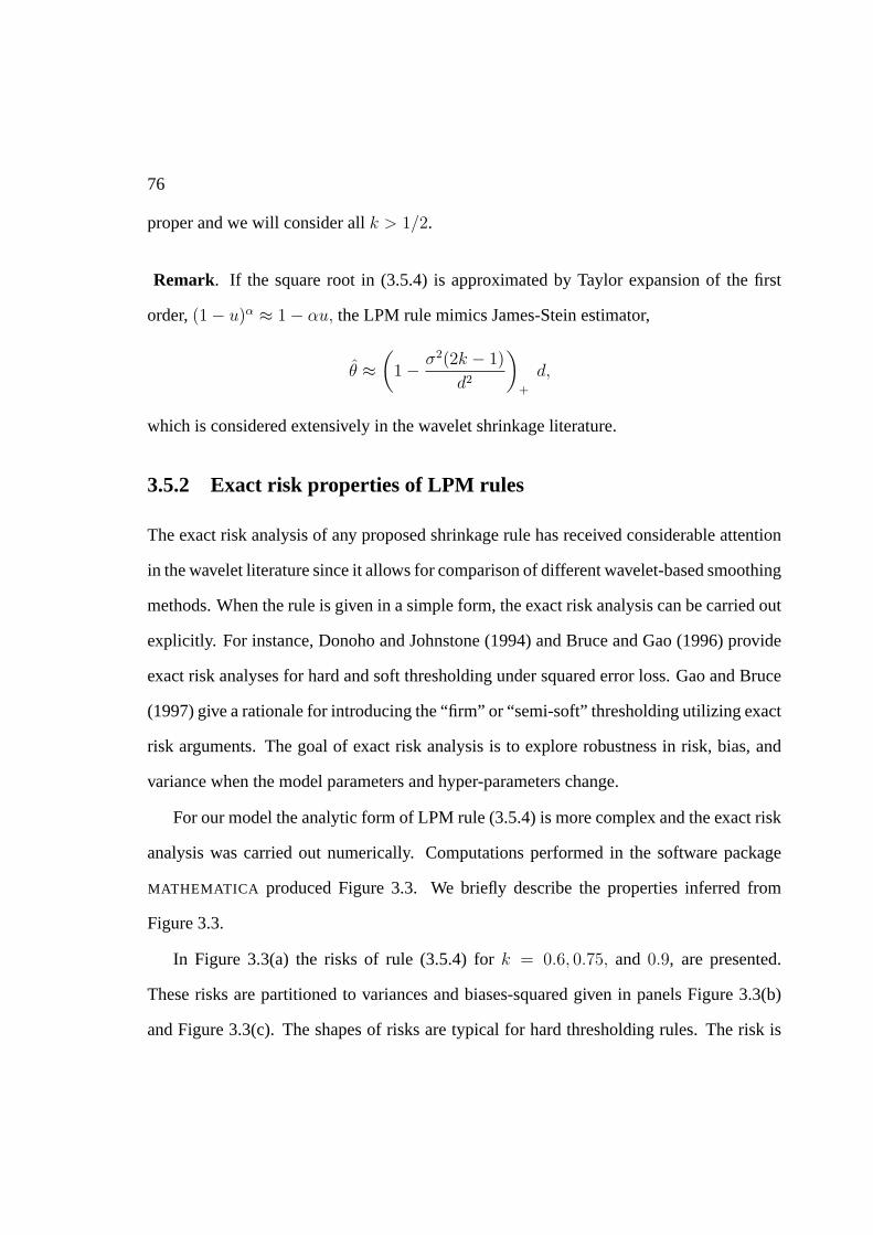
76
proper and we will consider allk > 1/2.
Remark. If the square root in (3.5.4) is approximated by Taylor expansion of the first
order,(1− u)α ≈ 1− αu, the LPM rule mimics James-Stein estimator,
θ ≈(
1− σ2(2k − 1)
d2
)
+
d,
which is considered extensively in the wavelet shrinkage literature.
3.5.2 Exact risk properties of LPM rules
The exact risk analysis of any proposed shrinkage rule has received considerable attention
in the wavelet literature since it allows for comparison of different wavelet-based smoothing
methods. When the rule is given in a simple form, the exact risk analysis can be carried out
explicitly. For instance, Donoho and Johnstone (1994) and Bruce and Gao (1996) provide
exact risk analyses for hard and soft thresholding under squared error loss. Gao and Bruce
(1997) give a rationale for introducing the “firm” or “semi-soft” thresholding utilizing exact
risk arguments. The goal of exact risk analysis is to explore robustness in risk, bias, and
variance when the model parameters and hyper-parameters change.
For our model the analytic form of LPM rule (3.5.4) is more complex and the exact risk
analysis was carried out numerically. Computations performed in the software package
MATHEMATICA produced Figure 3.3. We briefly describe the properties inferred from
Figure 3.3.
In Figure 3.3(a) the risks of rule (3.5.4) fork = 0.6, 0.75, and 0.9, are presented.
These risks are partitioned to variances and biases-squared given in panels Figure 3.3(b)
and Figure 3.3(c). The shapes of risks are typical for hard thresholding rules. The risk is
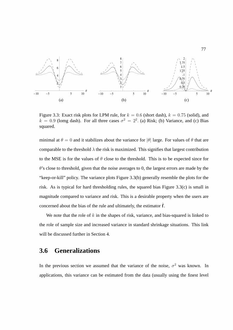
77
-10 -5 5 10Θ
2
4
6
8
-10 -5 5 10Θ
1
2
3
4
5
6
7
8
-10 -5 5 10Θ
0.25
0.5
0.75
1
1.25
1.5
1.75
2
(a) (b) (c)
Figure 3.3: Exact risk plots for LPM rule, fork = 0.6 (short dash),k = 0.75 (solid), andk = 0.9 (lomg dash). For all three casesσ2 = 22. (a) Risk; (b) Variance, and (c) Biassquared.
minimal atθ = 0 and it stabilizes about the variance for|θ| large. For values ofθ that are
comparable to the thresholdλ the risk is maximized. This signifies that largest contribution
to the MSE is for the values ofθ close to the threshold. This is to be expected since for
θ’s close to threshold, given that the noise averages to 0, the largest errors are made by the
“keep-or-kill” policy. The variance plots Figure 3.3(b) generally resemble the plots for the
risk. As is typical for hard thresholding rules, the squared bias Figure 3.3(c) is small in
magnitude compared to variance and risk. This is a desirable property when the users are
concerned about the bias of the rule and ultimately, the estimatorf .
We note that the role ofk in the shapes of risk, variance, and bias-squared is linked to
the role of sample size and increased variance in standard shrinkage situations. This link
will be discussed further in Section 4.
3.6 Generalizations
In the previous section we assumed that the variance of the noise,σ2 was known. In
applications, this variance can be estimated from the data (usually using the finest level
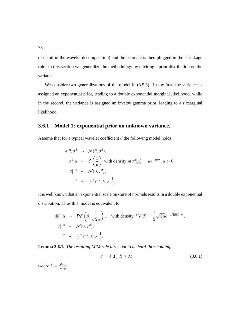
78
of detail in the wavelet decomposition) and the estimate is then plugged in the shrinkage
rule. In this section we generalize the methodology by eliciting a prior distribution on the
variance.
We consider two generalizations of the model in (3.5.3). In the first, the variance is
assigned an exponential prior, leading to a double exponential marginal likelihood, while
in the second, the variance is assigned an inverse gamma prior, leading to at marginal
likelihood.
3.6.1 Model 1: exponential prior on unknown variance.
Assume that for a typical wavelet coefficientd the following model holds.
d|θ, σ2 ∼ N (θ, σ2),
σ2|µ ∼ E(
1
µ
)with densityp(σ2|µ) = µe−µσ2
, µ > 0,
θ|τ 2 ∼ N (0, τ 2),
τ 2 ∼ (τ 2)−k, k >1
2.
It is well known that an exponential scale mixture of normals results in a double exponential
distribution. Thus this model is equivalent to
d|θ, µ ∼ DE(
θ,1√2µ
), with densityf(d|θ) =
1
2
√2µe−
√2µ|d−θ|,
θ|τ 2 ∼ N (0, τ 2),
τ 2 ∼ (τ 2)−k, k >1
2.
Lemma 3.6.1.The resulting LPM rule turns out to be hard-thresholding,
θ = d 1(|d| ≥ λ) (3.6.1)
whereλ = 2k−1√2µ
.

79
Proof. Proof of Lemma 3.6.1 is deferred to the Appendix
-1 1 2 3 4Θ
1
2
3
4
5
6
7
8
-1 -0.5 0.5 1d
-1
-0.5
0.5
1
(a) (b)
Figure 3.4: (a) Influence on the posterior in Model 1 by two different values ofd; (b) LPMrule for Model 1.
Figure 3.4(a) shows the posterior distribution for Model 1 for values ofd leading to
unimodal (infinite at mode 0) and bimodal cases. The values ared = 0.3 andd = 1.5,
k = 0.75 andµ = 1. The LPM rule (3.6.1) is shown in Figure 3.4(b) fork = 0.75 and
µ = 1/2.
The double exponential marginal likelihood is a realistic model for wavelet coefficients.
In fact, if a histogram of wavelet coefficients for many standard signals is plotted, it resem-
bles a double exponential distribution. This observation first explicitly stated by Mallat
(1989), is used in many Bayesian models in the wavelet domain, examples are BAMS
wavelet shrinkage (Vidakovic and Ruggeri, 2001) or the wavelet image processing method-
ology of Simoncelli and coauthors (e.g., Simoncelli and Adelson, 1996).

80
3.6.2 Model 2: inverse gamma prior on unknown variance.
The inverse gamma prior on the unknown variance of a normal likelihood is the most
common and well understood prior. The resulting marginal likelihood on the wavelet co-
efficients ist-distributed, which models heavy tails of empirical distributions of wavelet
coefficients well. Model 2 with an inverse gamma prior will not realistically model the
behavior of wavelet coefficients in the neighborhood of 0, but will account for heavy tails
encountered in empirical distributions of wavelet coefficients. Model 2 is given by
d|θ, σ2 ∼ N (θ, σ2),
σ2 ∼ IG(α, β) with densityp(σ2|α, β) =βα
Γ(α)(σ2)
−1−αe−β
σ2 , α > 0, β > 0,
θ|τ 2 ∼ N (0, τ 2),
τ 2 ∼ (τ 2)−k, k >1
2.
Lemma 3.6.2.The resulting LPM rule is
θ =(2α + 4k − 1)d + sign(d)
√(2α + 1)2d2 + 16(1− 2k)(k + α)β
4(k + α)1(|d| ≥ λ),(3.6.2)
where
λ =2
2α− 1
√(2k − 1)(k + α)β .
Proof. Proof of Lemma 3.6.2 is deferred to the appendix.
Figure 3.5(a) shows the posterior distribution for the Model 2 for values ofd leading to
unimodal and bimodal cases. The values are:d = 0.7 andd = 2.7, k = 0.85, α = 2.5 and
β = 2. The LPM rule (3.6.2) is shown in Figure 3.5(b) fork = 0.85, α = 2.5 andβ = 2.
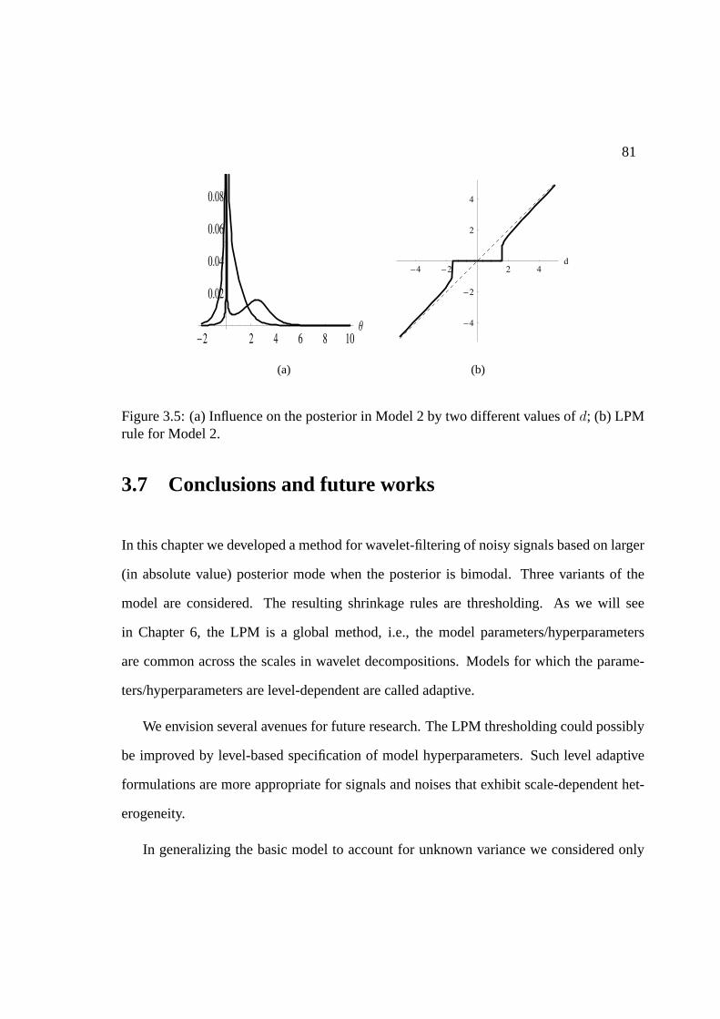
81
-2 2 4 6 8 10
Θ
0.02
0.04
0.06
0.08
-4 -2 2 4
d
-4
-2
2
4
(a) (b)
Figure 3.5: (a) Influence on the posterior in Model 2 by two different values ofd; (b) LPMrule for Model 2.
3.7 Conclusions and future works
In this chapter we developed a method for wavelet-filtering of noisy signals based on larger
(in absolute value) posterior mode when the posterior is bimodal. Three variants of the
model are considered. The resulting shrinkage rules are thresholding. As we will see
in Chapter 6, the LPM is a global method, i.e., the model parameters/hyperparameters
are common across the scales in wavelet decompositions. Models for which the parame-
ters/hyperparameters are level-dependent are called adaptive.
We envision several avenues for future research. The LPM thresholding could possibly
be improved by level-based specification of model hyperparameters. Such level adaptive
formulations are more appropriate for signals and noises that exhibit scale-dependent het-
erogeneity.
In generalizing the basic model to account for unknown variance we considered only

82
exponential and inverse gamma scale mixtures of normals. Scale mixtures of normals com-
prise a rich family of models and it would be possible to find an optimal mixing distribution.
Specifically, an exponential power distribution (EPD) that contains as special cases normal
and double exponential distributions can be obtained as a scale mixture of normals with
positive stable distribution as a mixing distribution.

Chapter 4
Numerical Experiments forDiscriminant Analysis
Introduction
In this chapter we apply some of the classification techniques introduced in chapter 1.
In section 4.1 Cloud detection from satellite multispectral images through statistical dis-
criminant analysis is investigated. Validation on case studies from the AVHRR sensor is
performed. In section 4.2 some local discriminant methods are tested on synthetic data,
performance of the different method are compared and suggestions for future work are
provided.
4.1 Multispectral cloud detection: general problem
Cloud detection is a preliminary important step in most algorithms for processing radiance
data measured from satellites. For this reason a cloud mask endows radiance data coming
from most last generation sensors onboard satellites. Practically all operative cloud mask
83

84
algorithms are physically based: cloud models are introduced in radiative transfer mod-
els and their influence on the radiance emitted from the Earth surface is estimated with
respect to clear sky conditions at spectral regions that simulate the spectral channels of a
sensor. Then generally single bands or couples of bands are considered and thresholds on
the value of radiances at the bands (or their differences or ratios, e.g.) are empirically cho-
sen able to discriminate between the clear and cloudy sky conditions. Such a procedure is
very consolidated and robust, especially when the type of clouds present in the atmosphere
matches the clouds that were simulated in the radiative models. Physical methodologies
suffer from three main drawbacks: the variability of clouds in the sky is much larger than
that resulting from simulations by radiative transfer models; the dependence of radiance
on the emissivity of the surface, which is very difficult to estimate accurately over land;
the increase of the number of spectral channels of sensors, that makes more difficult the
choice of suitable bands for the decision rules. For this reason there was in the recent
years interest towards classification methods that approach the problem of cloud detection
through statistical methods: the classification methods learn the statistical features of the
cloudy and clear sky conditions “on-field”, that is starting from “truth” images where the
sky conditions arecertainlyknown; then sky conditions on other “new” images are inferred
from these by relying on some of the statistical properties learned. However there is a main
drawback that limits evolution of this methodology into an operative algorithm.Supervised
classification methods rely on a “truth” cloud mask as a training set. Indeed at the same
time this is the strongest link of the (statistical) discriminant analysis to cloud physics. Ac-
tually to develop such a cloud mask is a hard task. Therefore a common procedure is to use
as a training set the result of classification obtained by a different methodology, in general
85
non based on pure statistical arguments. This weakens the role of the classification methods
as competitor of the physically based ones, since formally the final target of classification is
moved to reproduce the classification results of another methodology. Nevertheless, these
statistical approaches can shed more light on misclassifications of physical methods, by
looking deeply at the pixels classified differently between statistical and physical methods;
moreover they allow one to perform an assessment of the cloud detection methodology
with respect to the spectral bands, aimed at estimatingon field the role of each spectral
band and decision rule in the physical cloud detection methodology.
4.1.1 Classification methods considered
Three nonparametric (NPDA, PCDA, ICDA) and one parametric (LDA) discriminant anal-
ysis methods for multispectral cloud detection have been considered. These methods were
described in Chapter 1 and we briefly summarize them in the following. LDA (Linear Dis-
criminant Analysis) is based on Gaussian density functions with common variance among
classes; in NPDA (NonParametric Discriminant Analysis) a nonparametric estimate of the
density functions is made for each component separately; in PCDA (Principal Component
Discriminant Analysis) original components are transformed into principal components
prior to nonparametric density estimation; in ICDA (Independent Component Discrimi-
nant Analysis) original components are transformed into independent components prior to
nonparametric density estimation.

86
4.1.2 Case studies
We consider the NOAA/NASA Pathfinder AVHRR Land data set available at the NASA
Distributed Active Archive Center (DAAC) Web sitehttp://daac.gsfc.nasa.gov .
The Pathfinder AVHRR Land data sets are terrestrial data sets produced from 20 years of
archived data from the five-channel AVHRR sensor aboard the NOAA satellites. AVHRR
has five channels in the order: 0.58–0.68µm (visible), 0.725–1.10µm (near infrared),
3.55–3.93µm (middle infrared), 10.3–11.3 and 11.5–12.5µm (thermal).
We consider the Daily Data Set product, available at the resolution of 8 Km× 8 Km
that contains reflectances and radiances for the five channels and the Clouds from AVHRR
(CLAVR) product, seeAgbu and James(1994), for a detailed description of the products. In
particular CLAVR uses the five-channel multispectral information in a series of sequential
decision-tree type tests to identify the cloud-free, mixed (variably cloudy), and cloudy pix-
els. InStowe at al.(1991) it is claimed that the CLAVR technique is based on the following
differences between the radiative and physical properties of clouds and the underlying sur-
face: magnitudes of reflected and emitted radiation (contrast), wavelength dependence, and
spatial variability.
We consider two datasets (Jun 21, 2000 and Jun 21, 2001) and two experiments. In the
first one, data of June 21, 2000 are considered as a training and testing dataset. In the second
experiment data of June 21, 2001 are used as a training set, whereas data of June 21, 2000
are actually classified. In both cases training set is taken from the CLAVR product. An
area covering Mediterranean is considered (30o–50o latitude and 0o–40o longitude range)
that includes over 40000 useful pixels.
To rank the effectiveness of the discriminant analysis methods in detecting clouds, the

87
observed percentage of agreement,S, for the whole volume of data (the percentage of
correctly classified pixels) has been considered.
For each experiment, classification is performed by the four discriminant analysis meth-
ods discussed in Chapter 1. In addition, assessing of spectral bands is made considering all
their possible combinations (that is, cloud detection using just one band, two bands, and so
on). Therefore the total number of experiments for all combinations of bands is 31.
4.1.3 Results
First of all we show as an example in Fig. 4.1 typical probability density functions of clear
and cloudy sky reflectances in the spectral band 0.58–0.68µm over different zones in the
Mediterranean area on June 21, 2000. It is clear that hypothesis of Gaussianity of distribu-
tions is not met at all. The same result holds also for the other spectral bands. Therefore
it makes sense to consider discriminant analysis methods that estimate probability density
functions nonparametrically.
Table 4.1 shows performance of the discriminant analysis methods in terms of success
percentage (S) for the case when both training and testing datasets are given by the day
June 21, 2000.
We see that the thermal channels 4 and 5 (10.3–11.3µm and 11.5–12.5µm), taken inde-
pendently, give the best prediction, whereas band in the middle infrared (3.55–3.93µm) has
the poorest performance. It is also clear that nonparametric methods significantly improve
cloud detection capability. When bands are put together, we notice that detection capa-
bilities improve, as expected. In particular, the middle infrared spectral channel is always
present in all top performance combinations, that is it is the best companion spectral band.

88
Also noteworthy is that top performances are reached already with only two bands and that
differences of performance among the various methodologies tend to be small when the
number of channels increases — in other words multispectrality fixes the departure of data
from the theoretical assumptions of the methodology.
In order to test robustness of the methodology, we considered again June 21, 2000 as a
training set, but test was made on June 21, 2001. Table 4.2 shows performance of the Inde-
pendent Component Discriminant Analysis (the best performing). Findings of the previous
analysis were substantially confirmed and top performance is reduced only slightly.
4.2 Simulation of Local discriminant methods
This section includes results obtained applying on synthetic datasets the local discriminant
methods introduced in Chapter 1. We consider an image formed by a 100x100 array of
pixels. The image contains three distinct regions, each one populated according to a specific
probability density function, so that class labels are homogeneous inside each region. The
image is shown in Fig. 4.2. We assume that probability density function inside each region
is Gaussian with specified meanµk and varianceσ2k, k = 1, 2, 3.
We shall compare the four local classification methods proposed in chapter 1 (LV, LF,
LI and LN) with proper nonlocal methods and with ICM (Besag, 1986). To this purpose
we recall that ICM method assumes that the true label set of an image is a realization of a
locally dependent Markov Random field so that the posterior class probability for a specific
data point also depends on the labelling of its neighborhood. After obtaining a first class
estimates for each pixel using the classical Bayes rule (1.2.6) with constant a priori class
probabilities, at every iteration step and for each pixelxc the classes a priori probabilities

89
are estimated as follows:
πICMk (xc) =
exp(βϕk(xc))∑Kj=1 exp(βϕj(xc)
), k = 1, . . . , K, (4.2.1)
whereϕk(xc) are defined by Eq. (1.7.2), andβ is a fixed parameter that, when positive,
encourages the central pixel to have the same class as the dominant one in the neighbor-
hood. In our experiments we will setβ = 1.5 (for more details see Besag 1986). Notice
that by its very definition, namely the presence of the exponential term in Eq. (4.2.1), ICM
strongly privileges the most probable class according to the class labels estimated by some
discriminant analysis method; therefore it strongly enhances visibility of already visible
classes.
Example 1
In the first example we choose (µ1 = 1, σ21 = 1), (µ2 = 4, σ2
2 = 1) and (µ3 = 7, σ23 = 1).
As we can see from Figure 4.3, in this situation the three distributions overlap just on small
intervals so that all of them are veryvisible, in the sense that their dominance index is
high for all classes (0.9332, 0.8664 and 0.9332 for the three classes, respectively). As a
consequence all five local classification methods show a high global percentage of success
rate (see Table 4.3; digits are averages over 50 different realizations). We also compare
performance with a nonlocal method (Linear Discriminant Analysis, LDA), that is well
suited in this case, due to the Gaussian distributions and to equal variance for the three
classes. Constant priori class probabilities for all the three classes were chosen for LV,
LF, LN, LDA and ICM. Convergence was reached in less than 10 iterations. Moreover
final solution was quite robust with respect to the choice of the first-guess priori class
probabilities. The regionB was a square 3x3 around each pixel. Figure 4.4 shows the

90
reconstructed label field for one realization through (nonlocal) LDA. It is possible to note
the presence of the ‘pseudo-nuisance’ discussed in the paper. As a comparison, Figure 4.4
shows the reconstructed label field obtained through LV. In this case the ‘pseudo-nuisance’
practically disappeared. Also note that boundaries between regions of different classes are
well represented, which means that perfromance is excellent even whenB includes pixels
belonging to different classes.
Example 2
In the second example we choose (µ1 = 1, σ21 = 1), (µ2 = 2, σ2
2 = 4) and (µ3 = 3, σ23 = 1).
As we can see from Figure 4.6, in this situation the second distribution overlaps almost
everywhere with the others and it is lower, so that it is clearlynot visible. This is confirmed
also by the dominance index, which is 0.7973,0.0965 and 0.7973 for the three classes,
respectively. Table 4.4 shows classification success percentage for each class and globally
for the four local classification methods together with ICM and Quadratic Discriminant
Analysis (QDA); the latter is well suited in this example, due to the Gaussian distributions
and to different variances for the three classes. As it could have been expected, success
percentage is much lower, due to the very poor capability of all methods of predicting
class label 2. Figure 4.7 shows the reconstructed label field from one realization through
QDA. It is possible to note that class 2 in the middle region is very poorly predicted. As
a comparison, Figures 4.8 and 4.9 respectively show the reconstructed label field obtained
through LN and ICM. Note that as expected our proposed local methods LF, LI and LN
tend to privilege occurrence of the less visible classes, so that they perform better than
ICM and LV in these cases. As in example 1, the regionB was a square 3x3 around each

91
pixel.
4.2.1 Real data
Clouds are a typical example where it is difficult to set values to priori class probabilities,
because presence of clouds depends on the season, on the location and on the climate, all
items strongly varying with images. In addition clouds do show a strong spatial correlation,
just because from the physical point of view they are aggregation of water particles. Of
course the degree of correlation depends on the type of cloud and on the meteorological
conditions; in this respect an important role is also played by the spatial resolution of the
sensor that detects images from satellite. For this reason cloud mask detection is prone to
benefit from local algorithms for classification.
In this section we show an example of cloud mask retrieval for a scene over Italy of
September 21st 2000. Image was taken by MODIS sensor onboard NASA EOS satellite.
MODIS yields images in 36 spectral channels covering visible and near infrared spectral
regions, but only two of them have the best spatial resolution of 250m. For this reason it is
interesting to develop cloud mask algorithms that rely on a very limited number of spectral
channels, so that the cloud mask has the same best spatial resolution as the data and no
degradation to the resolution of other channels occurs.
Figure 4.10 shows the image considered in the present paper, which refers to reflectance
at the spectral channel 0.465µm. Discriminant analysis has been applied by means of the
NPDA (NonParametric Discriminant Analysis) method described in Amato et al., 2003.
In practice class distributions are estimated by means of Kernel density estimation, which
is appropriate for this problem since probability density functions of the clear and cloudy
92
classes cannot be approximated by Gaussian. Both the cases of nonlocal and local class
priori probabilities have been considered: in the first case uniform values over the classes
were considered; in the second case uniform values were used as first guess and LF method
was chosen to compute final localized values. The regionB was a square 3x3 around each
pixel. Results of classification are shown in Fig. 4.11. They confirm capability of the
localized discriminant analysis to reduce ‘pseudo-nuisance’ of nonlocal methods.
4.2.2 Conclusions
Some local discriminant analysis methods have been proposed for image classification
aimed at exploiting spatial correlation among neighbor pixels that is natural in most ap-
plications. These methods have the twofold objective of a) reducing the ‘pseudo-nuisance’
of nonlocal methods due to the overlap of the probability density functions of the various
classes; b) decrease misclassifications of even simple discriminant analysis methods, so
that performance are approached of more advanced methods even using very low dimen-
sional information for each pixel. The proposed methods are based on the choice of local
priori class probabilities using information surrounding each pixel of the image. Discrimi-
nant analysis has been revisited according to the visibility or nonvisibility of classes, that is,
capability of a particular classification method to retrieve a class. In these respect suitabil-
ity of the proposed methods to visible or nonvisible classes has been stressed. Particular
attention has been paid to the problem of detecting the cloud mask from satellite remote
sensed images, which is very important in remote sensing and seems particularly suited for
nonlocal discriminant analysis methods. Numerical experiments on synthetic datasets con-
firm performance improvement of the nonlocal methods with respect to the local ones. No

93
degradation is detected in proximity of the boundaries between regions of different classes.
Results for nonvisible classes show to be still poor. Therefore it is advisable to investigate
on alternative methods suited for both visible and nonvisible classes.

94
0 10 20 30 40 50 60 70 80 90 1000
0.05
0.1
0.15
0.2
0.25
0.3
0.35AVHRR − 0.58−0.68µm − Land−clear
Reflectance [%]
0 10 20 30 40 50 60 70 80 90 1000
0.02
0.04
0.06
0.08
0.1
0.12
0.14
0.16AVHRR − 0.58−0.68µm − Land−cloudy
Reflectance [%]
Figure 4.1: Typical density functions for clear and cloudy sky conditions.
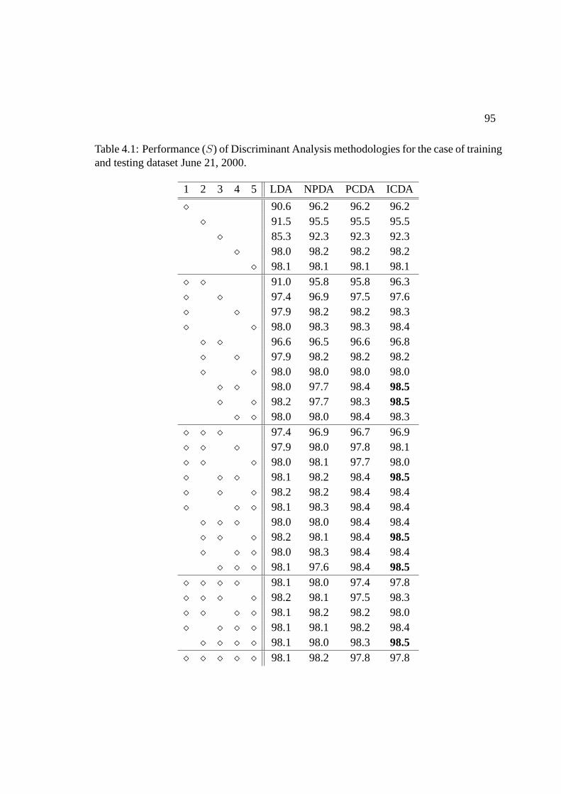
95
Table 4.1: Performance (S) of Discriminant Analysis methodologies for the case of trainingand testing dataset June 21, 2000.
1 2 3 4 5 LDA NPDA PCDA ICDA
¦ 90.6 96.2 96.2 96.2¦ 91.5 95.5 95.5 95.5
¦ 85.3 92.3 92.3 92.3¦ 98.0 98.2 98.2 98.2
¦ 98.1 98.1 98.1 98.1¦ ¦ 91.0 95.8 95.8 96.3¦ ¦ 97.4 96.9 97.5 97.6¦ ¦ 97.9 98.2 98.2 98.3¦ ¦ 98.0 98.3 98.3 98.4
¦ ¦ 96.6 96.5 96.6 96.8¦ ¦ 97.9 98.2 98.2 98.2¦ ¦ 98.0 98.0 98.0 98.0
¦ ¦ 98.0 97.7 98.4 98.5¦ ¦ 98.2 97.7 98.3 98.5
¦ ¦ 98.0 98.0 98.4 98.3¦ ¦ ¦ 97.4 96.9 96.7 96.9¦ ¦ ¦ 97.9 98.0 97.8 98.1¦ ¦ ¦ 98.0 98.1 97.7 98.0¦ ¦ ¦ 98.1 98.2 98.4 98.5¦ ¦ ¦ 98.2 98.2 98.4 98.4¦ ¦ ¦ 98.1 98.3 98.4 98.4
¦ ¦ ¦ 98.0 98.0 98.4 98.4¦ ¦ ¦ 98.2 98.1 98.4 98.5¦ ¦ ¦ 98.0 98.3 98.4 98.4
¦ ¦ ¦ 98.1 97.6 98.4 98.5¦ ¦ ¦ ¦ 98.1 98.0 97.4 97.8¦ ¦ ¦ ¦ 98.2 98.1 97.5 98.3¦ ¦ ¦ ¦ 98.1 98.2 98.2 98.0¦ ¦ ¦ ¦ 98.1 98.1 98.2 98.4
¦ ¦ ¦ ¦ 98.1 98.0 98.3 98.5¦ ¦ ¦ ¦ ¦ 98.1 98.2 97.8 97.8
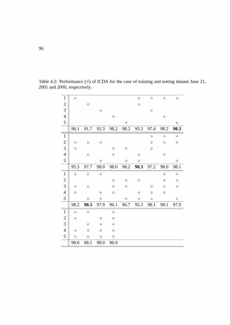
96
Table 4.2: Performance (S) of ICDA for the case of training and testing dataset June 21,2001 and 2000, respectively.
1 ¦ ¦ ¦ ¦ ¦2 ¦ ¦3 ¦ ¦4 ¦ ¦5 ¦ ¦
96.1 91.7 92.3 98.2 98.2 95.3 97.4 98.298.3
1 ¦ ¦ ¦2 ¦ ¦ ¦ ¦ ¦ ¦3 ¦ ¦ ¦ ¦4 ¦ ¦ ¦ ¦5 ¦ ¦ ¦ ¦
95.3 97.7 98.0 98.0 98.298.3 97.2 98.0 98.1
1 ¦ ¦ ¦ ¦ ¦2 ¦ ¦ ¦ ¦ ¦3 ¦ ¦ ¦ ¦ ¦ ¦ ¦4 ¦ ¦ ¦ ¦ ¦ ¦5 ¦ ¦ ¦ ¦ ¦ ¦
98.2 98.3 97.9 96.1 96.7 95.3 98.1 98.1 97.9
1 ¦ ¦ ¦2 ¦ ¦ ¦3 ¦ ¦ ¦4 ¦ ¦ ¦ ¦5 ¦ ¦ ¦ ¦
98.0 98.1 98.0 96.9

97
Figure 4.2: Image used for the synthetic experiments. Three regions are defined accordingto the color: 1 (black), 2 (gray) and 3 (white)
−4 −2 0 2 4 6 8 10 120
0.05
0.1
0.15
0.2
0.25
0.3
0.35
0.4class distibutions
123
Figure 4.3: Probability density functions for the first synthetic example.

98
C = 1 C = 2 C = 3 GlobalLDA 91.9 86.9 92.1 88.69ICM 99.5 99.8 99.4 99.65LV 99.5 99.5 93.5 98.13LF 97.3 95.9 97.2 96.35LI 96.6 95.3 97.1 95.85LN 98.6 97.5 98.0 97.77
Table 4.3: Success rate (percent) of discriminant analysis methods LF, LI, LN, ICM andLDA for the synthetic data of Example 1
Figure 4.4: LDA classification for the example 1. Colors are black for class 1, gray forclass 2 and white for class 3.
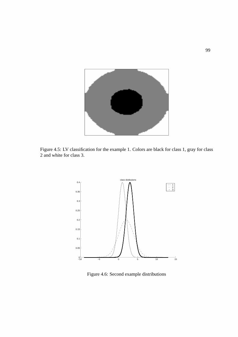
99
Figure 4.5: LV classification for the example 1. Colors are black for class 1, gray for class2 and white for class 3.
−10 −5 0 5 10 150
0.05
0.1
0.15
0.2
0.25
0.3
0.35
0.4class distibutions
123
Figure 4.6: Second example distributions
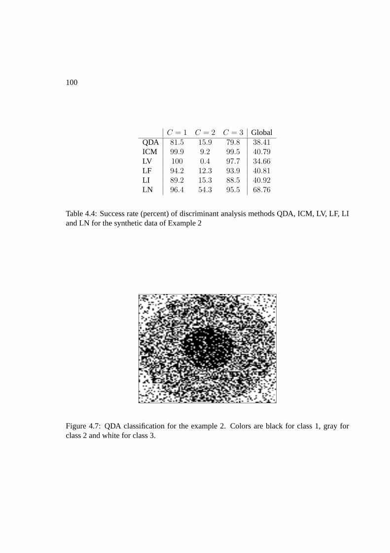
100
C = 1 C = 2 C = 3 GlobalQDA 81.5 15.9 79.8 38.41ICM 99.9 9.2 99.5 40.79LV 100 0.4 97.7 34.66LF 94.2 12.3 93.9 40.81LI 89.2 15.3 88.5 40.92LN 96.4 54.3 95.5 68.76
Table 4.4: Success rate (percent) of discriminant analysis methods QDA, ICM, LV, LF, LIand LN for the synthetic data of Example 2
Figure 4.7: QDA classification for the example 2. Colors are black for class 1, gray forclass 2 and white for class 3.
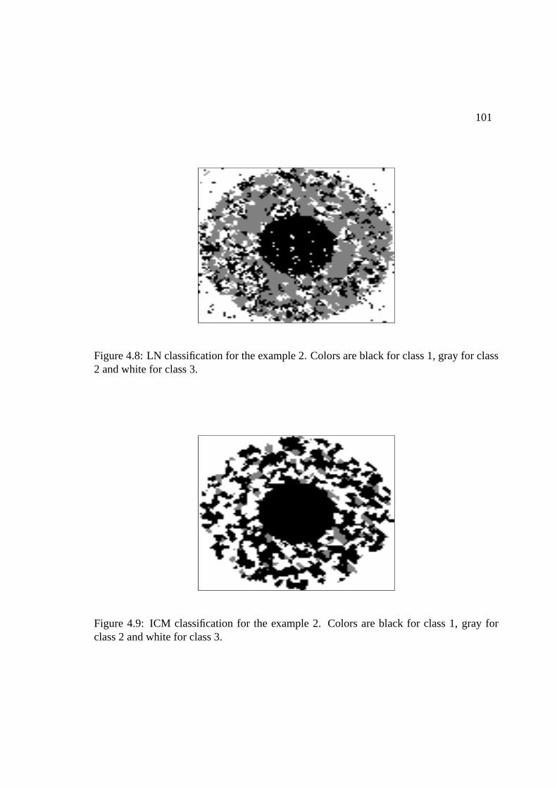
101
Figure 4.8: LN classification for the example 2. Colors are black for class 1, gray for class2 and white for class 3.
Figure 4.9: ICM classification for the example 2. Colors are black for class 1, gray forclass 2 and white for class 3.

102
Reflectance
Figure 4.10: Reflectance of MODIS spectral channel 0.465µm.
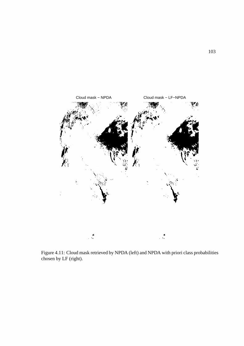
103
Cloud mask − NPDA Cloud mask − LF−NPDA
Figure 4.11: Cloud mask retrieved by NPDA (left) and NPDA with priori class probabilitieschosen by LF (right).

104
Chapter 5
Application of multiple testingprocedures to DNA microarray data
Introduction
In the present Chapter we give a brief introduction to cDNA microarray data and apply
some of the multiple testing procedures (MTP) described in Chapter 2 to a specific cDNA
microarray experimet . DNA microarray are part of a new class of biotechnology applica-
tions that allow the simultaneous monitoring of expression levels for thousands of genes in
cells. The main question in microarray experiments is the identification of the few genes
whose expression levels are associated with a response of interest, the so calleddiffer-
entially expressed genes. This biological question can be restated in terms of a multiple
hypotheses testing problem where for each gene the hypothesis of no association between
the expression levels and the response is tested.
The Chapter is organized as follows. Sections 1-3 provide a general background on DNA
microarray data. Section 4 describes different normalization methods to remove the source
of systematic variation in this kind of data. The application of MTP to a specific cDNA
105

106
microarray experiment is discussed in Section 5.
5.1 What is a microarray ?
One of the main purpose of genetic is finding functions of cells, comparing tissue types,
investigating the differences between healthy and diseased tissues, observing changes with
respect to the application of drugs for drug discovery, or monitoring treatments. In order
to reach these targets it is necessary to know the expression profiles of thousands of genes.
Trough the novel technology of DNA microarray it is now possible to obtain quantitative
measurements for the expression of genes present in a biological sample. The fundamen-
tal basis of DNA microarray is the process of hybridization. Two DNA strands hybridize
if they are complementary to each other. One or both strands of DNA can be replaced by
RNA and hybridization will still occur as long as there is complementarity. Roughly speak-
ing a microarray is a glass slide on which oligonucleotide probes have been immobilized at
micrometer distance. Small stings of RNA extracted from the sample of interest are used
to hybridize to complementary fragments of DNA immobilized on the chip. The sample
is usually labelled with a fluorescent dye so that the amount of hybridized mRNA can be
detected by a light scanner that scans the surface of the chip. Under the assumption that the
concentration of a particular messenger is a result of the expression of its corresponding
gene, the fluorescent intensity detected is used to estimate its relative expression level. This
application of DNA microarrays is in fact often referred to as expression analysis. Another
traditional and completely different application is the so called genotyping, which con-
sists in detecting mutation in specific genes. For expression analysis there are two major
technologies available: Affymetrix genechip and spotted arrays. Affymetrix uses masks to
107
control synthesis of oligonucleotides on the surface of a chip, divided in thousands of cells.
Each oligo is about 25 nucleotides long and up to 40 oligos are used for the detection of
each gene. Affymetrix chooses 11-20 oligos perfectly complementary, perfect match (PM),
to the mRNA of a specific region of a gene and 11-20 oligos miss match (MM) that are iden-
tical to the PM except for the central position where one nucleotide has been changed to its
complementary. The MM should be used to detect noise due to the process of hybridization
itself. Messenger RNA is extracted from a single sample cell and converted to complemen-
tary DNA (cDNA). It is then amplified, labelled and so ready to undergo fragmentation and
hybridization to the oligos on the surface of the chip. In spotted arrays technology a robot
spots small quantities of probes in solution to the surface of a glass where they are dried.
The probe can consist of cDNA, PCR (Polymerase Chain Reaction) or oligonucleotides.
Each probe is complementary to a unique gene in the genome. Spotted array are often used
to compare gene expression levels in two different samples, as the same cell type in two
different conditions, say healthy and diseased, or two different cell types. The mRNA is ex-
tracted from the two different samples cells, converted to cDNA and labelled fluorescently
with two dyes, usually red and green. After mixing they are hybridized to the probes on the
glass slide. In both cases, after the hybridization step, the unhybridized material is washed
away, the chip is scanned with a confocal laser and the image analyzed by computer. From
a data analysis point of view the main difference between the two technologies is that in
cDNA microarray two different samples labelled with two different dyes are hybridized on
the same chip whereas Affymetrix chip can handle only one fluorochrome so that two chips
are required to compare two samples. In the following we will focus on spotted arrays. The
108
raw data produced from microarray experiments are the hybridized images, typically 16-
bit TIFF (Tagged Information File Format), for each pair of sample to be compared. In
order to obtain a final gene expression matrix, these images should be segmented, each
spot identified, its intensity measured and compared to the background. This procedure is
called quantization and it is done by image analysis software by which data from a set of
microarray slides that constitute an experiment can be assembled into a single flat file. The
main quantities of are the (R, G) fluorescence intensity pairs for each gene in each array.
Note that since hereR will stand for red Cy5,G for green Cy3 and the DNA sequences
spotted on the array will be referred to as genes.
5.2 Experimental Design
Before a microarray experiment is performed, biological question to investigate on have
to be clear and so it is necessary to draw a specific experimental design. It is important
to decide whether a sample has to be considered as a biological replicate or a technical
replicate (obtained from the same biological source). The design is partially imposed by
the paired sample structure of two colors microarrays so that a single microarray can only
be used to compare directly two samples. The simplest design for the direct comparison
of two samples is the dye swap experiment. It uses two arrays to compare two samples
which are called control and treatment. If in array 1 control sample is assigned to the red
dye and treatment sample is assigned to the green dye, in array 2 the dye assignments are
reversed. Using biological replicates this arrangement can be repeated by any even num-
ber of arrays. This is called repeated dye swap experiment and it is useful for reducing
technical variation in the measurements. Using independent biological samples replicated

109
dye swap, experiment is obtained. This design accounts for both technical and biological
variation in the measurements. The most classical microarray experiments are based on
the reference design that employs a special RNA sample, called thereference, to whom
compare each test sample. Usually the reference is of no biological interest, so the number
of technical replicates available for inference is half of what we could get using a different
design. Even though this limitation, the reference design has the advantage of connecting
different samples through their comparisons to the same reference. The reference design
with dye swapping is a good design for large experiments because it is simple, robust and
the distance between samples is always two. Another experimental design is the so called
loop design in which samples are compared one to another in a daisy chain fashion. Small
loops are a good alternative to the reference design but large loops may be inefficient. Vari-
ations on this design can be achieved combining loops with reference design or multiple
loops together.
5.3 Expression Ratio
In a spotted cDNA microarray experiment, the ratio of the two fluorescent signals at each
spot is commonly used to infer the ratio of the mRNA concentrations in the two samples.
Lets consider an array that has N different genes and compare a samples1 labelled with red
dye, to a samples2 labelled with green dye. The ratio for thei-th gene is:Di = Ri
Gi. This is
commonly calledfold change. Intuitively the fold change gives a relative measurement of
how thei-th gene is expressed in samples1 with respect to samples2 that is ifDi is greater
then 1, thei-th gene is expressed more ins1 then ins2 and vice versa. In most experiments,
for the majority of genes, the ratio should be nearly one as no differential expression is
110
expected. Although the ratios give an intuitive way of measuring the relative genes expres-
sion level, it has the disadvantage of weighing up and down regulated genes differently. In
order to treat them symmetrically with respect to the non differentially expressed genes,
the logarithm of ratio is utilized to represent expression levels. Logarithm base 2 is used
instead of decimal or natural logarithm because intensity is typically an integer between
zero and216 − 1.
5.4 Normalization
In every microarray experiment it is important to take into account the systematic vari-
ation in the measured gene expression levels of two cohybridized mRNA samples so to
distinguish more easily biological differences and to allow comparison of expression levels
across the slides. The process of removing systematic effects due to non biological sources
is often referred to as normalization. There are many sources of systematic variation in
microarray data, including unequal quantities of starting RNA, differences in labelling,
different efficiency in the fluorescent dyes used, experimental bias in the measurements,
unbalanced scanners, experiments replicated in different conditions and so on. It is neces-
sary to normalize the fluorescent intensities before any analysis which involves comparing
expression levels within or between slides. In the following we will consider different
normalization methods.
5.4.1 Single slide data displays
Dudoit at al (2002) suggested that one of the most helpful graphical way of detecting
dependence of log ratios on fluorescent intensity, for each slide, is to represent the (R,G)
111
data trough plottingM = log2(R/G) versusA = log2[(RG)1/2]. This graphical method,
referred to as Ratio by Intensity (RI) plot or also MA-plot, is very useful for the purpose
of normalization. In fact, as underlined in the previous paragraph, under the assumption
that most genes are not differentially expressed and thata priori any differential expression
is approximately symmetric with respect to up and down regulated genes, most points in
an RI-plot should fall along a horizontal line. In practice this plot almost surely shows
different patterns.
5.4.2 Within slide normalization
Normalization issues associated with data obtained from a single slide is called within
slide normalization. The target of the within slide normalization is removing the eventual
curvature from the RI plot. There are several strategies that consist in subtracting a slide
specific function from the individual log ratios. Global, intensity dependent, within print
tip group and scale normalization will be provided in the following.
5.4.3 Global normalization
The simplest approach to within slide normalization is the global which consists in subtract-
ing a constant from all intensity log ratios, typically their mean or median. This method
assumes that red and green intensity are related by a constant factor and shifts to zero the
center of distribution of log ratio. For every genei on the array:
Ri = kGi ,
log2
(Ri
Gi
)½ log2
(Ri
Gi
)− c = log2
(Ri
kGi
)∀i ∈ = ,
where the set of index= denotes all the genes spotted on the array.
112
5.4.4 Intensity dependent normalization
In almost all experiments spatial or intensity dependent biases are evident so that an inten-
sity dependent normalization method is required. In the intensity dependent normalization
a local regression line is fitted to the MA plot via locally weighted least square methods,
lowess, and then the data are recentered along this line. The lowess function was first intro-
duced by Cleveland (1979) and it first appeared in microarray context in Luu at al (2001)
as a tool to normalize microarray data. Under the assumption that most genes are equally
expressed in both channels, the overall intensity level in the array can be approximated by
A, in fact for almost alli ∈ = :
log2(Ri) = log2(Gi) ½ Ai = log2[(RiGi)1/2] =
log2(Ri) + log2(Gi)
2= log2(Ri) = log2(Gi).
Fitting the lowess function c(A) to the MA plot leads to:
Ri = k(Ai)Gi,
Mi = log2
(Ri
Gi
)= log2[k(Ai)] = c(Ai) ½ k(Ai) = 2c(Ai) = ki.
Then the data will be corrected as follows:
log2
(Ri
Gi
)½ log2
(Ri
Gi
)− c(Ai).
This is equivalent to correct both channels intensity value as:
Ri → Ri,
Gi → k(Ai)Gi = kiGi.
While the global normalization method transforms all the genes using a unique value for
every slide, the lowess normalization appears most suitable to reduce the effect of the two
dyes.
113
5.4.5 Within print tip group normalization
Genes spotted on an array are grouped in grids. Every grid is printed using the same print
tip. The printing set up depends on the design and on the target of the experiment. The print
tips may be affected by systematic differences as unequal length of the tips or deformation
after many hours of printing and this may cause spatial effects on the slide. Thus it could
be necessary to apply a normalization depending both on intensity and on print tip group,
the so called within print tip group normalization:
log2
(Ri
Gi
)→ log2
(Ri
Gi
)− Cλ(Ai), ∀λ ∈ 1, . . . , Λ,∀i ∈ =λ,
whereCλ(.) is the lowess fit to the MA plot for theλ-th grid, Λ represents the number of
grids and=λ is the index set of the genes spotted in theλ-th grid.
5.4.6 Scale normalization
The log ratios from different grids, normalized by the within print tip group method, will
result centered around zero. Even if this behavior satisfy our first request, it is also neces-
sary that data from different print tip groups have the same spreadness. In order to reach
this goal a scale adjustment is required. An example of scale normalization can be obtained
under the assumption that log ratio data from thei-th grid are distributed as a Normal with
mean zero and variancea2i σ
2 wherea2i is the specific scale factor of thei-th print tip group
andσ2 is the true log ratio. The scale parameterai can be estimated via maximum likeli-
hood under the constraint∑Λ
=1 log(a2i ) = 0. Let ni be the number of genes in thei-th print
tip group and letMij = log(Ri
Gi) , i = 1, . . . , Λ andj = 1, . . . , ni. It results that
a2i =
∑ni
j=1 M2ij
(ΠΛi=1
∑ni
j=1 M2ij)
1/2.
114
5.4.7 Multiple slide normalization
Reguardless the normalization method used, in the within slide normalization step, the
normalized log ratio will turn out to be centered around zero. After this first step it is
necessary to make all the data from different slide comparable, in the sense that log ratios
from different slide should have similar spread. The target of multiple slide normalization
is just to allow comparisons between experiments. This kind of normalization may also be
performed using the method described in section 5.4.6.
5.5 Yeast experiment
5.5.1 Experiment description
In this section we describe a real data cDNA microarray experiment on the whole Yeast
genome. The aim of biologist’s study is to identify target genes, whose transcription acti-
vation is dependent on Cdk1. The starting point was to test Cdk 1’s role in recruiting the
SRB/Mediator and Pol II to the whole yeast genome. Wild type GAL-CDC20 and cdc28-13
GAL-CDC20 mutant cells were arrested in metaphase by incubating cells at the permissive
temperature (25 C) in medium lacking galactose. The cultures were then shifted to 37
to inactivate Cdk 1 and 20 minutes later were induced to enter G1 by the re-addiction of
galactose. The cdc28-13 mutants remained as unbudded cells failing to re-enter S phase. A
similar experiment was performed using SRB4-Myc GAL-CDC20 and SRB4-Myc cdc28-
13 GAL-CDC20. Samples were taken each 10-20 minutes starting from time point zero
(arrested cells) until 110 minutes after release. Cells were formaldehyde crosslinked and
distrupted with glass beads. After shearing of the chromatin by sonication, the crosslinked
DNA-protein complexes were immunoprecipitated either with the monoclonal antibody
115
anti Myc (9E11) to recover the SRB4’s associated chromatin fragments or with the mouse
monoclonal antibody 8WG16 against the C terminal domain of Rbp1 to recover PolII ’s as-
sociated chromatin fragments. The crosslinks were reversed by incubation at 65 C and the
recovered chromatin fragment purified. To control the efficiency of the experiments, PCR
amplification on the purified chromatin was performed to verify the association of known
target genes. The biologists want to analyze the genome wide association of metaphase ar-
rested cells (time point 0) of G1 cells (time point 40) and of cells either still arrested in G1
in the cdc28-13 mutant or already re-entered in the next cell cycle (time point 60 and 90).
The chromatin purified was analyzed from the time point 40. Chromatin fragments from
wild type GAL-CDC20 and cdc28-13 GAL-CDC20 and from SRB4-Myc GAL-CDC20
and SRB4- Myc cdc28-13 GAL-CDC20 were randomly amplified. Chromatin was first
amplified with degenerated tagged oligonucleotides by the use of the sequenase enzyme. A
PCR was then performed onto the obtained template using oligonucleotides complemen-
tary to the tag. Fragments ranging between 500 and 1000 bp were clearly visible onto
agarose gel after PCR amplification. To test the non-repetitively abundance of some PCR
amplified target genes with respect to others, we cloned the SRB4’s associated amplified
fragments in a T vector. Millions of colonies were obtained and we only 100 of them were
analyzed by sequence. Finally, the amplified chromatin samples were labelled with Cy3
and Cy5 fluorophores and combined two by two: samples from Srb4 IP together with sam-
ples from Srb4 cdc28-13 IP, and samples from Pol II IP together with samples from Pol II
cdc28-13 IP. The purified probes were hybridized to arrays containing 6400 yeast ORFs.
The main target of this experiment is to analyze the arrays and individuate genes which are
dependent or independent of Cdk1.

116
5.5.2 Methods
In this section we briefly describe the processing of the Yeast experiment data. For our
analysis purpose, we consider this experiment as consisting of two related sets of data:
SRB and POL II. The number of arrays employed to test the Cdk 1’s role is 6 for SRB and
9 for Pol II. Each array is a kind of treatmentvs control experiment, where the treatment is
the cell at the mutant stage, while the control is the cell at the wild type stage. The number
of technical replicates of each gene on each array is 2. The number of gene spotted on each
array ism=6400. After image processing and normalization step (see previous sections),
the gene expression data were summarized by a bi-dimensional array of log intensities
ratiosX of components,
Xji = log2
(WTji
MTji
), j = 1, . . . ,m i = 1, . . . , nj,
whereWTji andMTji are respectively the fluorescence intensities measuring the ex-
pression level of the genej spoti, in the wild type condition and in the mutant condition.
We measure each gene spot expression level, both inWT andMT , by the average back-
ground corrected fluorescence intensity.
We want to find out the genes that are not differentially expressed, betweenWT and
MT , in SRB and that, at the same time, are over expressed inWT with respect toMT in
POL II. We formulate this problem in terms of multiple hypothesis testing and we compare
different strategies to reach our goal. The basic idea is to:
1. Consider at-statisticTj for each genej
Tj =√
nXj − θj
Sj
,
117
where the gene standard deviation,Sj, is opportunely estimated from the data (different
corrections were also considered.
2.Choose a multiple testing procedure (MTP) to test on the SRB dataset, simultaneously
for each genej, the following assumption
H0j : θj 6= 0 vs H1j : θj = 0 , (5.5.1)
whereθj denotes the expression level of genej. Let G be the set of gene selected by the
choosenMTP .
3. Choose a MTP to test on the POL II dataset, simultaneously for each genej in G, the
following assumption
H0j : θj = 0 vs H1j : θj > 0. (5.5.2)
The resulting selected genes are then considered the target genes of the described Yeast
experiment. We tried different way to implement these three steps. In the step 1, three
different estimates ofSj were considered: the sample standard deviation, a SAM like esti-
mate (see Tusheret al, 2001) and a percentile estimate (see Efronet al, 2001). For the SRB
dataset we used the MAP and theempiricalMTP, described in Chapter 2. For the POL II
dataset we adopted the MAP MTP. Note that the Bayesian testing approach assumes the
normal distribution on the error term. Such assumption is often criticized when microar-
ray data are considered. In order to avoid this assumption we consider also an empirical
approach on SRB, which is similar in spirit to the MAP MTP; i.e. we select as non differ-
entially expressed in SRB those genes whose|Ti| is lower then a user selected threshold.
As a second stage a frequentist adaptive FDR controlling procedure is used.P -values are

118
estimated by resampling methods (see Section 2.4). For each choice lists of genes where
obtained and the common genes were selected. These different strategies were chosen
indifferently and the resulting lists of genes were compared. The common genes were se-
lected. The results were almost stable in a number of about fifty genes. Positive controls in
the literature database were found. The biologists are now analyzing the final list of genes
in order to confirm the findings.
Chapter 6
LPM: simulations, comparisons and reallife example
Introduction
In this chapter we apply the thresholding rules proposed in chapter three. In the first Section
we discuss the selection of the hyperparameters for each model. This is important for an
automatic application of the methodology. In the first Section we compare performance
of the proposed rules to eight other commonly used methods (both global and adaptive).
In the last Section we apply the shrinkage methodology to a real-life example involving
Atomic Force Microscopy.
6.1 Selection of hyperparameters
In any Bayesian modeling task the selection of the hyperparameters is instrumental for
good performance of the model. It is also desirable to have an automatic way to select the
hyperparameters, thus making the shrinkage procedure automatic, i.e., free of subjective
119

120
user intervention. More about specification of hyperparameters in Bayesian models in the
wavelet denoising context can be found in Chipman, Kolaczyk, and and McCulloch (1997),
Vidakovic and Ruggeri (2001), and Angelini and Sapatinas (2004), among others.
The hyperparameters should be selected so that the resulting methodology is robust
with respect to a wide range of input signals (sample sizes, signal regularity, size of noise,
etc). In contemporary wavelet practice the values of the hyperparameters are usually as-
sessed by empirical Bayes arguments due to enormous variability of potential input data
(Clyde and George, 1999; 2000). Straightforward Empirical Bayes techniques such as pre-
dictive moment matching, or MLII method, are most commonly used efficient methods
for hyperparameter specification. In this paper we determine hyperparameters by moment-
matching.
In chapter three we considered three Bayesian models on wavelet coefficients, (i) the
basic model withσ2 assumed known, and two generalizations in which the varianceσ2 is
modeled by (ii) exponential and (iii) inverse-gamma priors. In this section the elicitation
of corresponding hyperparameters is discussed for each case.
The Basic Model. In the basic model the only hyperparameter is thepower parameterk.
Even though the proper posterior is obtained fork < 1, the existence of the second, non-
zero mode does not depend on the “properness” of the posterior. Thus we will consider
all k > 1/2. Note that the conditionk > 1/2 is needed to ensure that Gamma function
Γ(2k − 1) is finite and non-negative.
The sample size of the input signal should influence our selection ofk. Figure 6.1 shows
the Bumps signal at SNR =5 and sample sizesn = 512, 1024, 2048, and4096, smoothed by
LPM thresholding rule (3.5.4) for various values ofk. The minimum average mean square
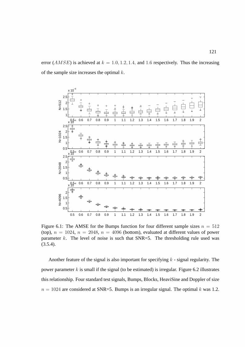
121
error (AMSE) is achieved atk = 1.0, 1.2, 1.4, and1.6 respectively. Thus the increasing
of the sample size increases the optimalk.
0.5 0.6 0.7 0.8 0.9 1 1.1 1.2 1.3 1.4 1.5 1.6 1.7 1.8 1.9 2
1
1.5
2
2.5
x 10−4
N=
51
2
0.5 0.6 0.7 0.8 0.9 1 1.1 1.2 1.3 1.4 1.5 1.6 1.7 1.8 1.9 20.5
1
1.5
2
2.5x 10
−4
N=
10
24
0.5 0.6 0.7 0.8 0.9 1 1.1 1.2 1.3 1.4 1.5 1.6 1.7 1.8 1.9 20.5
1
1.5
2
2.5x 10
−4
N=
20
48
0.5 0.6 0.7 0.8 0.9 1 1.1 1.2 1.3 1.4 1.5 1.6 1.7 1.8 1.9 2
0.5
1
1.5
2
x 10−4
N=
40
96
Figure 6.1: The AMSE for the Bumps function for four different sample sizesn = 512(top), n = 1024, n = 2048, n = 4096 (bottom), evaluated at different values of powerparameterk. The level of noise is such that SNR=5. The thresholding rule used was(3.5.4).
Another feature of the signal is also important for specifyingk - signal regularity. The
power parameterk is small if the signal (to be estimated) is irregular. Figure 6.2 illustrates
this relationship. Four standard test signals, Bumps, Blocks, HeaviSine and Doppler of size
n = 1024 are considered at SNR=5. Bumps is an irregular signal. The optimalk was 1.2.
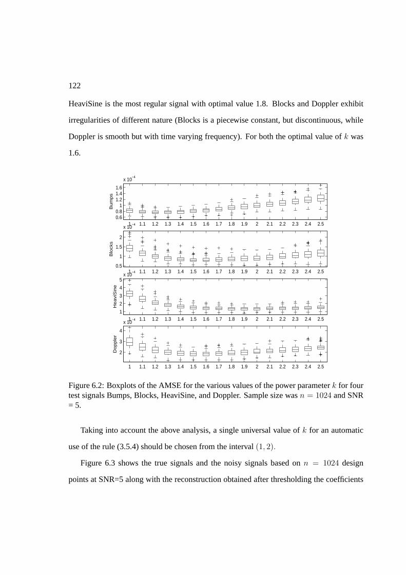
122
HeaviSine is the most regular signal with optimal value 1.8. Blocks and Doppler exhibit
irregularities of different nature (Blocks is a piecewise constant, but discontinuous, while
Doppler is smooth but with time varying frequency). For both the optimal value ofk was
1.6.
1 1.1 1.2 1.3 1.4 1.5 1.6 1.7 1.8 1.9 2 2.1 2.2 2.3 2.4 2.50.60.8
11.21.41.6
x 10−4
Bu
mp
s
1 1.1 1.2 1.3 1.4 1.5 1.6 1.7 1.8 1.9 2 2.1 2.2 2.3 2.4 2.50.5
1
1.5
2
x 10−4
Blo
cks
1 1.1 1.2 1.3 1.4 1.5 1.6 1.7 1.8 1.9 2 2.1 2.2 2.3 2.4 2.51
2
3
4
5x 10
−4
He
avi
Sin
e
1 1.1 1.2 1.3 1.4 1.5 1.6 1.7 1.8 1.9 2 2.1 2.2 2.3 2.4 2.5
2
3
4
x 10−4
Do
pp
ler
Figure 6.2: Boxplots of the AMSE for the various values of the power parameterk for fourtest signals Bumps, Blocks, HeaviSine, and Doppler. Sample size wasn = 1024 and SNR= 5.
Taking into account the above analysis, a single universal value ofk for an automatic
use of the rule (3.5.4) should be chosen from the interval(1, 2).
Figure 6.3 shows the true signals and the noisy signals based onn = 1024 design
points at SNR=5 along with the reconstruction obtained after thresholding the coefficients

123
0 0.2 0.4 0.6 0.8 10.1
0.2
0.3
0.4
0.5
0.6
0.7
0.8Bumps
0 0.2 0.4 0.6 0.8 10.1
0.2
0.3
0.4
0.5
0.6
0.7
0.8Blocks
0 0.2 0.4 0.6 0.8 10
0.2
0.4
0.6
0.8
1HeaviSine
0 0.2 0.4 0.6 0.8 10
0.2
0.4
0.6
0.8
1Doppler
0 0.2 0.4 0.6 0.8 10.1
0.2
0.3
0.4
0.5
0.6
0.7
0.8Bumps
0 0.2 0.4 0.6 0.8 10.1
0.2
0.3
0.4
0.5
0.6
0.7
0.8Blocks
0 0.2 0.4 0.6 0.8 10.1
0.2
0.3
0.4
0.5
0.6
0.7
0.8HeaviSine
0 0.2 0.4 0.6 0.8 10.1
0.2
0.3
0.4
0.5
0.6
0.7
0.8Doppler
(a) (b)
Figure 6.3: (a) Test signals with superimposed noisy versions at SNR=5. The sample sizeis n = 1024. (b) Estimates obtained by using the LPM method with optimalk.
by LPM method with optimalk. we can see that LPM method does a very good job at
removing the noise. From Figure 6.4 we can see the change in smoothness of recovered
signals with the change ofk.
Model 1. In the model with an exponential prior onσ2 in addition to the power parameter
k we also have the hyperparameterµ which is the reciprocal of the scale parameter. Given
an estimatorξ of the noise variance, a moment-matching choice forµ would beµ = 1
ξ.
Donoho and Johnstone (1994) suggested to estimate the noise levelσ by the median abso-
lute deviation (MAD) of the wavelet coefficients at the finest level adjusted by 1/0.6745,
our choice is to considerξ = MAD 2. In this model we will considerk > 1/2 with no
upper bounds because, even if the posterior distribution is not proper, the choice ofk > 1
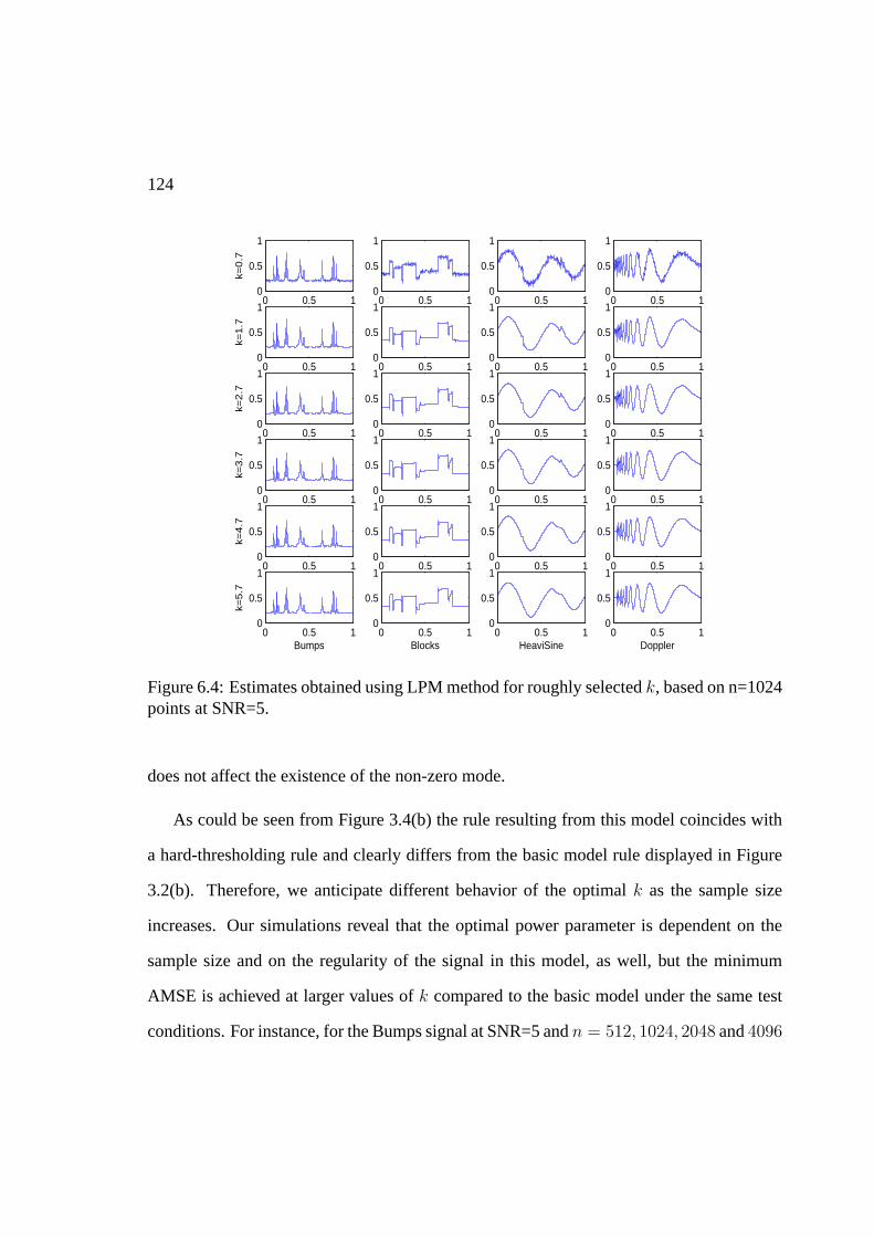
124
0 0.5 10
0.5
1k=
0.7
0 0.5 10
0.5
1
k=1.7
0 0.5 10
0.5
1
k=2.7
0 0.5 10
0.5
1
k=3.7
0 0.5 10
0.5
1
k=4.7
0 0.5 10
0.5
1
k=5.7
Bumps
0 0.5 10
0.5
1
0 0.5 10
0.5
1
0 0.5 10
0.5
1
0 0.5 10
0.5
1
0 0.5 10
0.5
1
0 0.5 10
0.5
1
Blocks
0 0.5 10
0.5
1
0 0.5 10
0.5
1
0 0.5 10
0.5
1
0 0.5 10
0.5
1
0 0.5 10
0.5
1
0 0.5 10
0.5
1
HeaviSine
0 0.5 10
0.5
1
0 0.5 10
0.5
1
0 0.5 10
0.5
1
0 0.5 10
0.5
1
0 0.5 10
0.5
1
0 0.5 10
0.5
1
Doppler
Figure 6.4: Estimates obtained using LPM method for roughly selectedk, based on n=1024points at SNR=5.
does not affect the existence of the non-zero mode.
As could be seen from Figure 3.4(b) the rule resulting from this model coincides with
a hard-thresholding rule and clearly differs from the basic model rule displayed in Figure
3.2(b). Therefore, we anticipate different behavior of the optimalk as the sample size
increases. Our simulations reveal that the optimal power parameter is dependent on the
sample size and on the regularity of the signal in this model, as well, but the minimum
AMSE is achieved at larger values ofk compared to the basic model under the same test
conditions. For instance, for the Bumps signal at SNR=5 andn = 512, 1024, 2048 and4096
125
the optimal values ofk are2.1, 2.4, 2.6 and2.8, respectively, while for the four standard
test signals Bumps, Blocks, HeaviSine and Doppler of sizen = 1024 at SNR=5 the optimal
values ofk are2.4, 2.7, 3.0 and2.7. Therefore, for an automatic use of the thresholding rule
in the exponential model, a single universal value ofk should be selected from the interval
(2, 3).
Model 2. In the model with an inverse gamma prior onσ2 in addition to the power param-
eterk we also have two new hyperparametersα andβ which specify the prior. As in Model
1 we will match the prior moments with the observed moments in order to specify the hy-
perparameters. Then-th moment of an inverse gamma random variableX ∼ IG(α, β)
is
EXn =βn
(α− 1) . . . (α− n).
Thus, the first two moments matched with the corresponding empirical moments of wavelet
coefficients from the finest level of detail will “estimate”α andβ. This consideration and
Gaussianity of the noise yieldsα = 2.5 andβ = 1.5 ξ, whereξ is some estimator of the
variance of the noise. As in the previous models we use the robust(MAD)2 estimator. An
argument for the specification ofα andβ are given in the Appendix.
As in the previous two cases, we anticipate different behavior of the optimalk with
respect to the sample size and regularity of test functions. For instance, forα = 2.5 and
β determined usingα and an estimator of the variance of the noise for Bumps signal with
SNR = 5 the AMSE minimizing values ofk are 1.3, 1.6, 1.8, and 2.0 for sample sizes
512, 1024, 2048, and 4096, respectively. For the four standard test signals Bumps, Blocks,
HeaviSine and Doppler of sizen = 1024 at SNR=5 the optimal values ofk are1.6, 2.0, 2.3
126
and2.0. Therefore, for an automatic use of the thresholding rule in the inverse gamma
model, a single universal value ofk should be selected from the interval(1, 3).
6.2 Simulations and comparisons
We present a simulation study of the performance of LPM method for the three models.
The simulation is done with the “known truth”, that is with test functions specified, and
controlled signal-to-noise ratio. We also compare the average mean square error (AMSE)
performance with several popular methods.
For our simulation study, four standard test functions (Bumps, Blocks, HeaviSine
andDoppler ) were added rescaled normal noise to produce a preassigned signal-to-noise
ratio (SNR). For each method, test functions were simulated atn = 512, 1024, and 2048
points equally spaced on the unit interval. Three commonly used SNR’s were selected:
SNR=3 (weak signal), 5 (moderate signal), and 7 (strong signal). The wavelet bases are
also standard for the above test functions: Symmlet 8 forHeaviSine andDoppler ,
Daubechies 6 forBumpsand Haar forBlocks .
Closeness of the reconstruction to the theoretical signal of each method was measured
by an average mean-square error (AMSE), calculated over 1000 simulation runs. In each
case, the optimal power parameterk (minimizing AMSE) was used. All computations
are carried out using MATLAB, with the WaveLab toolbox (see Buckheit, Chen, Donoho,
Johnstone, and Scargle, 1995) and the GaussWaveDen toolbox (see Antoniadis, Bigot, and
Sapatinas, 2001).
The results are summarized in two tables. Table 6.1 gives minimum AMSE for the three
introduced models at three SNR levels and for four standard test functions, while Table 6.2

127
presents the corresponding optimal value of the power parameterk.
Final Results× 10−3
Function n SNR=3 SNR=5 SNR=7
Bumps 512 0.2825 0.3116 0.2875 0.1079 0.1180 0.1095 0.0570 0.0621 0.05771024 0.1953 0.2150 0.1993 0.0733 0.0802 0.0745 0.0373 0.0401 0.03792048 0.1254 0.1371 0.1282 0.0469 0.0509 0.0477 0.0240 0.0257 0.0244
Blocks 512 0.3820 0.4111 0.3876 0.1202 0.1265 0.1213 0.0553 0.0568 0.05541024 0.2752 0.3004 0.2790 0.0802 0.0827 0.0800 0.0359 0.0364 0.03572048 0.1584 0.1692 0.1601 0.0480 0.0502 0.0483 0.0201 0.0204 0.0200
HeaviSine 512 0.4066 0.4305 0.4155 0.2243 0.2441 0.2300 0.1432 0.1575 0.14721024 0.2769 0.2966 0.2835 0.1353 0.1443 0.1379 0.0890 0.0964 0.09142048 0.1711 0.1786 0.1734 0.0950 0.1007 0.0969 0.0604 0.0666 0.0622
Doppler 512 0.7046 0.7706 0.7187 0.2725 0.2959 0.2767 0.1449 0.1557 0.14701024 0.4491 0.4879 0.4590 0.1896 0.2062 0.1931 0.1032 0.1125 0.10542048 0.2514 0.2649 0.2540 0.1064 0.1135 0.1081 0.0596 0.0639 0.0607
Table 6.1: AMSE for the Basic Model (left), Model 1 (center), and Model 2 (right) atdifferent SNR levels and for the four standard test functions.
We also compare LPM method with several established wavelet-based estimators for re-
constructing noisy signals. In particular we consider the term-by-term Bayesian estimator
BAMSof Vidakovic and Ruggeri (2001), the classical term-by-term estimatorsVisuShrink
of Donoho and Johnstone (1994) andHybrid-SureShrinkof Donoho and Johnstone (1995),
the scale invariant term-by-term BayesianABEmethod of Figueiredo and Nowak (2001),
the “leave-out-half” version of theCross-Validationmethod of Nason (1996), the term-by-
term False Discovery Rate (FDR) method of Abramovich and Benjamini (1995), and finally
NeighCoeffof Cai and Silverman (2001) andBlockJSof Cai (1999) which represent clas-
sical estimators that incorporate the blocking procedure to achieve a better performance.
Note that, for excellent numerical performance, we consider theVisuShrinkand the “leave-
out-half” version of theCrossValidationmethods with the hard threshold and theBlockJS
with the option ’Augment’ (see Antoniadis, Bigot, and Sapatinas, 2001).
The LPM is a global method, i.e., the model parameters/hyperparameters are common
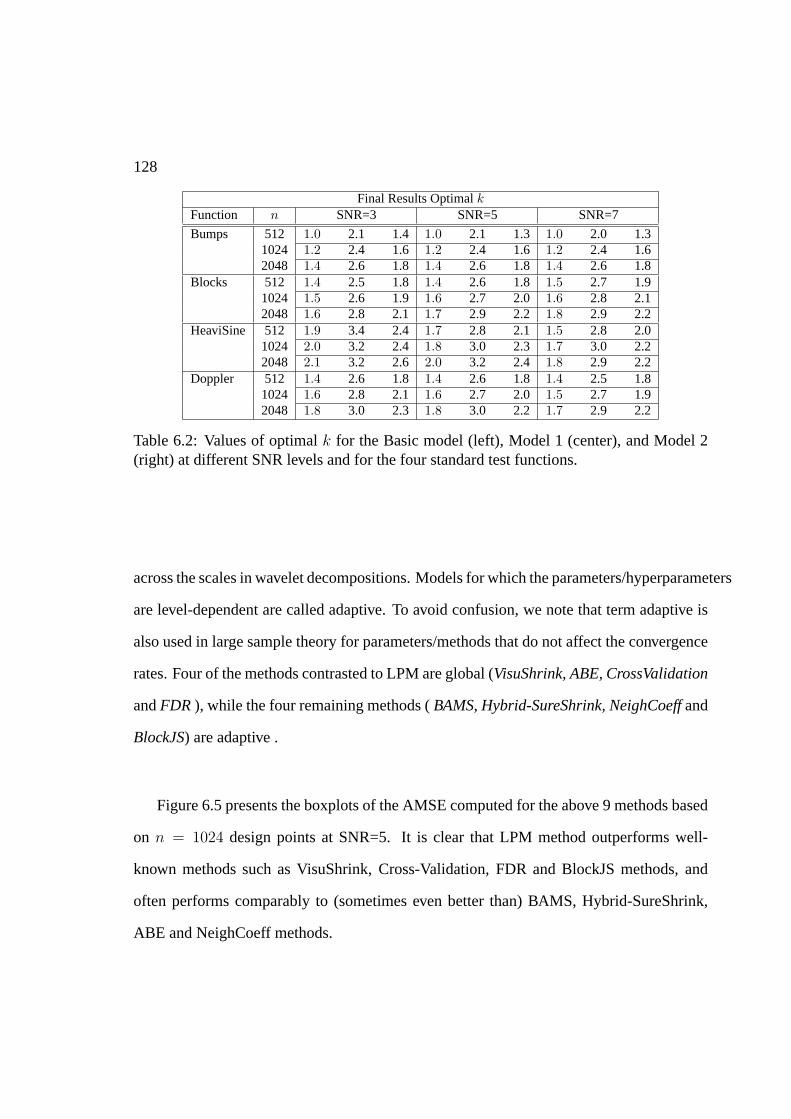
128
Final Results OptimalkFunction n SNR=3 SNR=5 SNR=7
Bumps 512 1.0 2.1 1.4 1.0 2.1 1.3 1.0 2.0 1.31024 1.2 2.4 1.6 1.2 2.4 1.6 1.2 2.4 1.62048 1.4 2.6 1.8 1.4 2.6 1.8 1.4 2.6 1.8
Blocks 512 1.4 2.5 1.8 1.4 2.6 1.8 1.5 2.7 1.91024 1.5 2.6 1.9 1.6 2.7 2.0 1.6 2.8 2.12048 1.6 2.8 2.1 1.7 2.9 2.2 1.8 2.9 2.2
HeaviSine 512 1.9 3.4 2.4 1.7 2.8 2.1 1.5 2.8 2.01024 2.0 3.2 2.4 1.8 3.0 2.3 1.7 3.0 2.22048 2.1 3.2 2.6 2.0 3.2 2.4 1.8 2.9 2.2
Doppler 512 1.4 2.6 1.8 1.4 2.6 1.8 1.4 2.5 1.81024 1.6 2.8 2.1 1.6 2.7 2.0 1.5 2.7 1.92048 1.8 3.0 2.3 1.8 3.0 2.2 1.7 2.9 2.2
Table 6.2: Values of optimalk for the Basic model (left), Model 1 (center), and Model 2(right) at different SNR levels and for the four standard test functions.
across the scales in wavelet decompositions. Models for which the parameters/hyperparameters
are level-dependent are called adaptive. To avoid confusion, we note that term adaptive is
also used in large sample theory for parameters/methods that do not affect the convergence
rates. Four of the methods contrasted to LPM are global (VisuShrink, ABE, CrossValidation
andFDR ), while the four remaining methods (BAMS, Hybrid-SureShrink, NeighCoeffand
BlockJS) are adaptive .
Figure 6.5 presents the boxplots of the AMSE computed for the above 9 methods based
on n = 1024 design points at SNR=5. It is clear that LPM method outperforms well-
known methods such as VisuShrink, Cross-Validation, FDR and BlockJS methods, and
often performs comparably to (sometimes even better than) BAMS, Hybrid-SureShrink,
ABE and NeighCoeff methods.
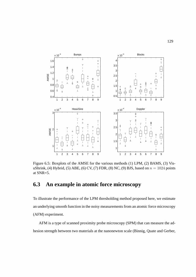
129
1 2 3 4 5 6 7 8 90.4
0.6
0.8
1
1.2
1.4
1.6
x 10−4 Bumps
AM
SE
1 2 3 4 5 6 7 8 90.5
1
1.5
2
2.5
3
3.5
4
x 10−4 Blocks
1 2 3 4 5 6 7 8 9
1
2
3x 10
−4 HeaviSine
AM
SE
1 2 3 4 5 6 7 8 9
1
1.5
2
2.5
3
3.5x 10
−4 Doppler
Figure 6.5: Boxplots of the AMSE for the various methods (1) LPM, (2) BAMS, (3) Vis-uShrink, (4) Hybrid, (5) ABE, (6) CV, (7) FDR, (8) NC, (9) BJS, based onn = 1024 pointsat SNR=5.
6.3 An example in atomic force microscopy
To illustrate the performance of the LPM thresholding method proposed here, we estimate
an underlying smooth function in the noisy measurements from an atomic force microscopy
(AFM) experiment.
AFM is a type of scanned proximity probe microscopy (SPM) that can measure the ad-
hesion strength between two materials at the nanonewton scale (Binnig, Quate and Gerber,
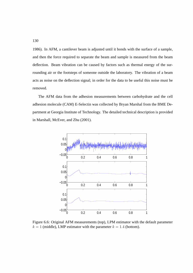
130
1986). In AFM, a cantilever beam is adjusted until it bonds with the surface of a sample,
and then the force required to separate the beam and sample is measured from the beam
deflection. Beam vibration can be caused by factors such as thermal energy of the sur-
rounding air or the footsteps of someone outside the laboratory. The vibration of a beam
acts as noise on the deflection signal; in order for the data to be useful this noise must be
removed.
The AFM data from the adhesion measurements between carbohydrate and the cell
adhesion molecule (CAM) E-Selectin was collected by Bryan Marshal from the BME De-
partment at Georgia Institute of Technology. The detailed technical description is provided
in Marshall, McEver, and Zhu (2001).
0 0.2 0.4 0.6 0.8 1−0.05
0
0.05
0.1
0 0.2 0.4 0.6 0.8 1−0.05
0
0.05
0.1
0 0.2 0.4 0.6 0.8 1−0.05
0
0.05
0.1
Figure 6.6: Original AFM measurements (top), LPM estimator with the default parameterk = 1 (middle), LMP estimator with the parameterk = 1.4 (bottom).

131
In Figure 6.6 the top panel shows the original noisy data. The middle panel shows
the LPM estimate with the default parameterk = 1, while the bottom panel shows LPM
estimate with the parameterk = 1.4. The sample size wasn = 211 and Symmlet8-tap
filter was used to obtain the estimate. We observe that the latter estimate exhibits slightly
smoother behavior, especially in the long-middle part without oversmoothing the “ramp-
like” structure which is the feature of interest here.
We adhere to the concept of reproducible research (Buckheit and Donoho, 1995). The
m-files used for calculations and figures in this work can be downloaded from Jacket’s
Wavelets pagehttp://www.isye.gatech.edu/˜brani/wavelet.html .

132

Appendix A
A.1 Proof of Lemma (3.6.1)
Assume that for a typical wavelet coefficientd the following model holds.
d|θ, σ2 ∼ N (θ, σ2),
σ2 ∼ E(
1
µ
)with densityp(σ2|µ) = µe−µσ2
, µ > 0,
θ|τ 2 ∼ N (0, τ 2),
τ 2 ∼ (τ 2)−k, k >1
2.
It well known that the marginal likelihood, as a scale mixture of normals, is
d|θ ∼ DE(
θ,1√2µ
), with densityf(d|θ) =
1
2
√2µe−
√2µ|d−θ|.
Therefore the model can be rewritten as
d|θ ∼ 1
2
√2µe−
√2µ|d−θ|,
θ|τ 2 ∼ N (0, τ 2),
τ 2 ∼ (τ 2)−k,1
2.
133

134
The joint distribution ofd andθ is proportional to
p(d, θ) ∝∫ ∞
0
p(d|θ)p(θ|τ 2)p(τ 2)dτ 2
=1
2
õ
πe−
√2µ|d−θ|
∫ ∞
0
e−θ2/(2τ2) 1
(τ 2)kdτ 2
=1
2
õ
πe−
√2µ|d−θ|
∫ ∞
0
y(k−1/2)−1e−θ2y/2dy
=1
2
õ
πe−
√2µ|d−θ|Γ
(k − 1
2
)(θ2
2
)1/2−k
, k > 1/2.
Furthermore we have
p(θ|d) ∝ p(d, θ) ∝ e−√
2µ|d−θ|(θ2)1/2−k
.
The likelihood ofθ
l(θ) = e−√
2µ|d−θ|(θ2)1/2−k
(A.1.1)
is integrable if and only ifk < 1.
The eventual modes of the posteriorp(θ|d) exist if and only if they maximize the func-
tion (A.1.1), that is if and only if they maximizeL(θ) = log[l(θ)]. More explicitly
L(θ) = log[l(θ)] = −√
2µ|d− θ|+ 1− 2k log θ. (A.1.2)
Consider its derivative
L′ =√
2µ sign(d− θ) +1− 2k
|θ| sign(θ) =√
2µ sign(d− θ) +1− 2k
θ, (A.1.3)
and WLOG, supposed > 0. Observe that the critical points of (A.1.3) areθ1 = 0 and
θ2 = λ = 2k−1√2µ
.Whend < λ there exists only one mode in zero. Whend > λ there exists
two modes, the smaller is zero and the larger isd; in fact the function (A.1.2) is decreasing
between zero and lambda, increasing between lambda andd and decreasing afterd.

135
A.2 Proof of lemma (3.6.2)
The model considered was
d|θ, σ2 ∼ N (θ, σ2),
σ2 ∼ IG(α, β) with densityp(σ2|α, β) =βα
Γ(α)(σ2)
−1−αe−β
σ2 , α > 0, β > 0,
θ|τ 2 ∼ N (0, τ 2),
τ 2 ∼ (τ 2)−k, k >1
2.
It is well known thatt distribution is a scale mixture of normals, with mixing distribution
being an inverse gamma.
d|θ ∼ 1√2βB(1
2, α)
[(d− θ)2
2β+ 1
]−α− 12
, whereB(
1
2, α
)=
Γ(12)Γ(α)
Γ(12
+ α).
Therefore the model can be rewritten as
d|θ ∼ 1√2βB(1
2, α)
[(d− θ)2
2β+ 1
]−α− 12
, α > 0, β > 0,
θ|τ 2 ∼ N (0, τ 2),
τ 2 ∼ (τ 2)−k,1
2.

136
The joint distribution ofd andθ is proportional to
p(d, θ) ∝∫ ∞
0
p(d|θ)p(θ|τ 2)p(τ 2)dτ 2
=
∫ ∞
0
1√2βB(1
2, α)
[(d− θ)2
2β+ 1
]−α− 12 1√
2πτ 2e−θ2/(2τ2) 1
(τ 2)kdτ 2
=1
2√
βπB(12, α)
[(d− θ)2
2β+ 1
]−α− 12∫ ∞
0
(τ 2)−(k+1/2)e−θ2/(2τ2)dτ 2
=1
2√
βπB(12, α)
[(d− θ)2
2β+ 1
]−α− 12∫ ∞
0
y(k−1/2)−1e−θ2y/2dy
=1
2√
βπB(12, α)
Γ
(k − 1
2
)(θ2
2
)1/2−k [(d− θ)2
2β+ 1
]−α− 12
, k > 1/2
Furthermore, we have
p(θ|d) ∝ p(d, θ) ∝ |θ|1−2k[(d− θ)2 + 2β]−α−1/2.
The likelihood ofθ
l(θ) = |θ|1−2k[(d− θ)2 + 2β]−α−1/2, (A.2.1)
is integrable for anyk > 12.
The eventual modes of the posteriorp(θ|d) exist if and only if they maximize the function
(A.2.1). Since
l′ = (1− 2k)|θ|−2k sign(θ)[(d− θ)2 + 2β]−α−1/2 + |θ|1−2k(2α + 1)(d− θ)[(d− θ)2 + 2β]−α−3/2
= |θ|−2k sign(θ)[(d− θ)2 + 2β]−α−3/2(1− 2k)[(d− θ)2 + 2β] + (2α + 1)(d− θ)θ,

137
it follows that
|θ|−2k > 0,∀θ ∈ R− 0,
sign(θ) > 0,∀θ > 0,
[(d− θ)2 + 2β]−α−3/2
> 0,∀θ ∈ R,
and
l′ = 0 ⇔ (1− 2k)[(d− θ)2 + 2β] + (2α + 1)(d− θ)θ = 0,
with solutions
θ1,2 =(2α + 4k − 1)d±
√(2α + 1)2d2 + 16(1− 2k)(k + α)β
4(k + α).
The roots are real if and and only if(2α + 1)2d2 + 16(1− 2k)(k + α)β > 0 , i.e.,
|d| ≥ λ =2
2α− 1
√(2k − 1)(k + α)β . (A.2.2)
If the condition (A.2.2) is not satisfied then the MAP is given byθ = 0 . Now assume
that (A.2.2) holds andd > 0. In this case both solutionsθ1,2 are real and positive and the
posterior is decreasing from zero to the smaller root, increasing between the two roots and
decreasing again after the larger root. We have two posterior modes, the smaller is zero and
the larger is
θ =(2α + 4k − 1)d +
√(2α + 1)2d2 + 16(1− 2k)(k + α)β
4(k + α).
It is easy to see thatθ is always smaller thend, resulting in a shrinkage rule.
138
A.3 Selection of hyperparametersα and β in Model 2.
Note that for wavelet coefficients(d1, . . . , dm) from the finest level of detail the mean is
close to 0,d ≈ 0. That means thats2d = 1
m−1
∑(di−d)2 and 1
m
∑d2
i = d2 are both compa-
rable estimators of the variance. Also, even central empirical moments are approximately
equal to the noncentral moments. The following two equations are approximately moment
matching:
d2 =β
α− 1, d4 =
β2
(α− 1)(α− 2),
whered4 = 1m
∑d4
i . From these equations we derive
α =2d4 − (d2)2
d4 − (d2)2,
which is free of the scale of wavelet coefficients. Since in the finest level of detail the
contribution of signal is minimal and the wavelet coefficients are close to zero-mean normal
random variables the Law of Large Numbers argument givesd2 ≈ σ2 andd4 ≈ 3σ4, which
specifies the “shape” hyperparameter
α = 2.5.
Hyperparameterβ is determined fromd2 = βα−1
, but instead ofd2 we can use any estimator
of variance ofd. In simulations, we used the robust(MAD)2.

Bibliography
139
140
Abramovich, F. and Angelini, C. (2005). Bayesian Maximum a Posteriori Multiple Testing
Procedure. Technical Report, RP-SOR-05-01, Department of Statistics and Operations
Research, Tel Aviv University.
Abramovich, F. and Benjamini, Y. (1995). Thresholding of wavelet coefficients as multiple
hypotheses testing procedure. InWavelets and Statistics(Antoniadis A. & Oppenheim
G. Eds.) Lect. Notes Statist.103, 5-14, Springer-Verlag, New York.
Abramovich, F. and Sapatinas, T. (1999). Bayesian approach to wavelet decomposition and
shrinkage. InBayesian Inference in Wavelet Based Models, (Muller, P. & Vidakovic,
B. Eds.) Lect. Notes Statist.141, 33–50, Springer-Verlag, New York.
Agbu, P. A. and James, M. E. (1994). NOAA/NASA Pathfinder AVHRR Land Data Set
Users Manual, Goddard Distributed Active Archive Center, NASA Goddard Space
Flight Center, Greenbelt.
Amato, U., Antoniadis, A. and Gregoire, G. (2003). Independent Component Discriminant
Analysis. Int. J. Mathematics 3 735-753.
Angelini, C. and Sapatinas, T. (2004) Empirical Bayes approach to wavelet regression using
e-contaminated priors.Journal of Statistical Computation and Simulation, 74, 741 –
764.
Angelini, C. and Vidakovic, B. (2004).Γ-Minimax Wavelet Shrinkage: A Robust Incorpo-
ration of Information about Energy of a Signal in Denoising Applications,Statistica
Sinica,14, 103–125.
Antoniadis, A., Bigot, J. and Sapatinas, T. (2001). Wavelet estimators in nonparametric
regression: a comparative simulation study. J. Statist. Soft.6, 1–83.
Benjamini, Y. and Hochberg, Y. (1995).Controlling the false discovery rate: A practical
and powerful approach to multiple testing. Journal of the Royal Statistical Society
(Ser. B), 57, 289-300.
Benjamini, Y. and Yekutieli, D. (2001).The control of the false discovery rate in multiple
testing under dependency. Annals of Statistics, 29, 11651188.

141
Benjamini, Y. Reiner,A. and Yekutieli, Y. (2003).Identifying differentially expressed genes
using the FDR. Bioinformatics 19(3) 368-375.
Berger, J. O. (1985).Statistical Decision Theory and Bayesian Analysis. Second Edition.
Springer, New York.
Besag J. (1996).On Statistical Analysis of Dirty Pictures. J. R. Statistical Society Series B
48 (3).
Binnig, G., Quate, C.F., and Gerber, Ch. (1986). Atomic force microscope.Phys. Rev.
Lett. 56, 930–933.
Bruce, A.G., and Gao, H-Y., (1996). Understanding WaveShrink: Variance and bias esti-
mation. Biometrika83, 727–745.
Buckheit, J.B., Chen, S., Donoho, D.L., Johnstone, I.M. and Scargle, J. (1995). About
WaveLab. Technical Report, Department of Statistics, Stanford University, USA.
Buckheit, J. and Donoho, D. L. (1995). Wavelab and reproducible research, inWavelets
and Statistics, A. Antoniadis and G. Oppenheim eds., LNS 103, Springer-Verlag, New
York.
Cai, T.T. (1999). Adaptive wavelet estimation: a block thresholding and oracle inequality
approach. Ann. Statist.27, 898–924.
Cai, T.T. and Silverman, B.W. (2001). Incorporating information on neighbouring coeffi-
cients into wavelet estimation. Sankhya B, 63, 127–148.
Chen, J. and Sakar, S K. (2004).A Bayesian Stepwise Multiple Testing Procedure. Techni-
cal Report, Temple University.
Chipman, H.A., Kolaczyk, E.D. and McCulloch, R.E., (1997) Adaptive Bayesian wavelet
shrinkage. J. Amer. Stat. Assoc.92, 1413-1421.
Cleveland, W. S. (1979).Robust locally weighted regression and smoothing scatterplots.
Journal of American Statistical Association, 74, 829–836.
Clyde, M. and George, E.I. (1999). Empirical Bayes estimation in wavelet nonparametric
regression. InBayesian Inference in Wavelet Based Models, (Muller, P. & Vidakovic,

142
B. Eds.), Lect. Notes Statist.,141, pp. 309–322, Springer-Verlag, New York.
Clyde, M. and George, E.I. (2000). Flexible empirical Bayes estimation for wavelets. J. R.
Statist. Soc. B,62, 681–698.
Clyde, M., Parmigiani, G. and Vidakovic, B. (1998). Multiple shrinkage and subset selec-
tion in wavelets. Biometrika85, 391–401.
Cover, T. and Thomas, J. (1991).Elements of Information Theory. John Wiley and Sons,
Inc., New York.
Cutillo, L. and Amato, U. (2005).Local Discriminant Analysis for cloud detection. Pro-
ceeding from Cladag, University of Parma, italy.
Cutillo, L., Amato, U., Antoniadis, A., Cuomo, V. and Serio, C. (2004). Cloud detection
from multispectral satellite images. Proceedings from IEEE Gold Conference, Univer-
sity Parthenope, Naples, Italy.
Cutillo, L., Jung, Y. Y. , Ruggeri, F. and Viadakovic, B. (2005). Larger Posterior Mode
Wavelet Thresholding and Applications. Tecnical Report. RT 29705. Istituto per le
Applicazioni del Calcolo ”Mauro Picone” (IAC), Naples, Italy.
Donoho, D.L. and Johnstone, I.M. (1994). Ideal spatial adaptation by wavelet shrinkage.
Biometrika81, 425–455.
Donoho, D.L. and Johnstone, I.M. (1995). Adapting to unknown smoothness via wavelet
shrinkage. J. Am. Statist. Assoc.90, 1200–1224.
Donoho, D.L., Johnstone I., Kerkyacharian G. and Picard D. (1995). Wavelet shrinkage:
asymptopia J.Roy. Statist. Soc. B57, 301-370.
Duda, O. R., Hart, P. E. and Stork, D. G. (2001). Pattern Classification. Second Edition.
Wiley-Interscience.
Dudoit, S., Shaffer, P. J. and J.C. Boldrick (2003a).Multiple hypothesis testing in microar-
ray experiments. Statistical Science, 18, 71-103.
Efron, B., (1979).Bootstrap methods: another look at the jackknife. Ann. Statist. 7, 1-26.

143
Efron, B., Tibshirani, R.J., (1993).An Introduction to the Bootstrap. Chapman and Hall,
London.
Efron, B., Tibshirani, R., Storey, J. D. and Tusher, V. (2001).Empirical Bayes analysis of
a microarray experiment. Journal of the American Statistical Association, 96, 1151-
1160.
Figueidero, M.A.T. and Nowak, R.D. (2001). Wavelet-based image estimation: an empiri-
cal Bayes approach using Jeffrey’s noninformative prior. IEEE Trans. Image Process.
10, 1322–1331.
Gao, H-Y., and Bruce, A.G., (1997) WaveShrink with firm shrinkage. Statistica Sinica7,
855-874.
Genovese, C. R. and Wasserman, L. (2002).Operating characteristics and extensions of
the FDR procedure. Journal of the Royal Statistical Society (Ser. B), 64, 499518.
Ju, J., Gopal, S., and Kolaczyk, E.D. (2005).On the choice of spatial and categorical
scale in remote sensing land cover characterization. Remote Sensing of Environment,
96(1):62-77.
Benjamini,Y. and Hochberg,Y. (1995) Controlling the false discovery rate: a practical and
powerful approach to multiple testing. J. Roy. Stat. Soci. B, 57, 289300.
Hochberg, Y. (1988)a sharper Bonferroni procedure for multiple tests of significance.
Biometrika, 75, 800-803.
Hochberg, Y. and Benjamini Y. (1990).More powerful procedures for multiple significance
testing. Statistics in Medicine, 9, 811-818.
Hochberg Y. and Tamhane A. C. (1987).Multiple Comparisons Procedures. Wiley.
Hollander, M. and Wolfe, D. A. (1999). Nonparametric Statistical Methods. Second Edi-
tion. Wiley Series in Probability and Statistics.
Holm, S. (1979). A simple sequentially rejective multiple test procedure. Scandinavian
Journal of Statistics, 6, 65-70.
144
Hyvarinen, A. (1997). Independent component analysis by minimization of mutual infor-
mation, Proc. IEEE Int. Conf. on Acoustics, Speech and Signal Processing (ICASSP
97), 39173920.
Huber, P. J. (1981).Robust Statistics. Wiley Series in Probability and Statistics.
Johnstone, I. M. and Silverman, B. W. (2005). Empirical BAyes selection of wavelet thresh-
olds. The Annals of Statistics, Vol. 33, No. 4, 1700-1752.
Jolliffe, I. T. (2002). Principal Component Analysis. Second Edition. Springer Series in
Statistics.
Johnson, R. A. and Wichern, D. W. (1998). Applied Multivariate Statistical Analysis,
Fourth Ed., Prentice Hall, Upper Saddle River, NJ.
Keuchel, J., Naumann, S., Heiler, M., et al. (2003)Automatic land cover analysis for
Tenerife by supervised classification using remotely sensed data. REMOTE SENS
ENVIRON 86 (4): 530-541.
Khedama, R. and Belhadj-Aissaa, A. (2004). CONTEXTUALClassification of Renotely
Sensed Data Using MAP Approach and MRF. Proceedings from Instambul ISPRS
2004. Vol. XXXV, part B7
Mallat, S. G. (1989). A Theory for Multiresolution Signal Decomposition: The Wavelet
Representation.IEEE Trans. Pattern Analysis Machine Intel., 11, 674–693.
Marshall, B., McEver, R. and Zhu, C. (2001). Kinetic rates and their force dependence on
the P-Selectin/PSGL-1 interaction measured by atomic force microscopy. Proceedings
of ASME 2001, Bioengineering Conference, BED - Vol. 50.
Muller, P. and Vidakovic, B. (1999). MCMC methods in wavelet shrinkage. In:Bayesian
Inference in Wavelet-Based Models.Editors Muller, P. and Vidakovic, B., Springer-
Verlag, Lecture Notes in Statistics141, 187–202.
Nason, G.P. (1996).Wavelet shrinkage using cross-validation. J. R. Statist. Soc. B,58,
463–479.

145
Pensky, M. and Sapatinas, T. (2005). Frequentist optimality of Bayes factor estimators in
wavelet regression models. Technical Report, TR082005, Department of Mathematics
and Statistics, University of Cyprus, Cyprus.
Pollard, K. S. and Van der Laan, M. J. (2003).Resampling-based multiple testing: Asymp-
totic control of type I error and applications to gene expression data. Tech. Rep. 121
, Division of Biostatistics, UC Berkeley.
Ripley, B. D. (1996). Pattern Recognition and Neural Network. Cambridge University
Press.
Robbins, H. (1951).Asymptotically sub-minimax solutions to compound statistical deci-
sion problems. In Proc. Second Berkeley Symposium Math. Statist. and Prob. 1,
241-251. Berkeley University of California Press.
Ruggeri, F. and Vidakovic, B. (2005),Bayesian modeling in the wavelet domain, to appear
in Handbook of Statistics - vol. 25 - Bayesian Thinking, Modeling and Computation,
D. Dey and C.R. Rao, Eds., North Holland.
Sidak, Z (1967). Rectangular confidence regions for the means of multivariate normal
distributions. Journal of the American Statistical Association, 62, 626-633.
Sidak, Z. (1971).On probabilities of rectangles in multivariate Student distributions: their
dependence on correlations. Annals of Mathematical Statistics, 42, 169-175.
Silverman, B. W. (1986).Density estimation for Statistics and Data Analysis. Chapman
and Hall, London.
Simoncelli, E. and Adelson, E. (1996). Noise removal via Bayesian Coring,Proceedings
of 3rd IEEE International Conference on Image Processing, Vol. I, pp. 379–382.
Lausanne, Switzerland. 16-19 September 1996.
Scott, D. W. (1992).Multivariate Density Estimation: Theory, practice, and Visualization.
Wiley, New York.
Storey, J.D. and Tibshirani, R. (2001). Estimating false discovery rates under dependence,
with applications to DNA microarrays. Tech. Rep. 2001-28 , Department of Statistics,
146
Stanford University.
Stowe, L. L., McClain, L. L., Carey, R., Pellegrino, P., Gutman, G. G., Davis, P., Long, C.
and Hart, S (1991). Global distribution of cloud cover derived from NOAA/AVHRR
operational satellite data, Adv. Space Research 3, 51 54.
Tusher, Tibshirani and Chu (2001).Significance analysis of microarrays applied to the ion-
izing radiation response. PNAS 2001 98: 5116-5121.
Van der Laan, M. J., Dudoit, S. and Pollard, K. S. (2003).Multiple testing. Part II. Step-
down procedures for control of the family-wise error rate. Tech. Rep. 139 , Division
of Biostatistics, UC Berkeley.
Yang, Y. H., Dudoit, S., Luu, P., Lin, D. M., Peng, V. Ngai, J. and Speed, T. (2002).Nor-
malization for cDNA microarray data: a robust composite method addressing single
and multiple slide systematic variation. Nucleic Acids Research, Vol. 30, No.4 e15.
Yang, Y. H., Dudoit, S., Luu, P. and Speed T. P. (2001).Normalization for cDNA Microar-
ray Data. SPIE BiOS, San Jose, California.
Vidakovic, B., (1998). Non linear wavelet shrinkage with Bayes rules and Bayes factors.
J. Amer. Stat. Soc.45B, 173-179.
Vidakovic, B. (1999). Statistical Modeling by Wavelets. Wiley, New York.
Vidakovic, B. and Ruggeri, F. (1999). Expansion estimation by Bayes rules,J. Stat. Plann.
Infer.,79,223–235.
Vidakovic, B. and Ruggeri, F. (2001). BAMS Method: Theory and Simulations. Sankhya
B 63, 234–249.
Wand, M. P. and Jones, M. C. (1995). Kernel Smoothing. First Edition. Chapman and
Hall.
Westfall, P. H. and Young, S. S. (1993).Resampling-based Multiple Testing: Examples and
Methods for p-value Adjustment. Wiley.