classification errors in regression models: a … international is a trade name of research triangle...

RTI International is a trade name

of Research Triangle Institute www.rti.org

Classification Errors in Regression

Models:

A Bayesian Semi-Parametric Approach Presented by

Martijn van Hasselt

RTI International

Presented at

The 139th Annual Meeting of the American Public Health Association

Washington, DC • October 29–November 2, 2011

Phone 919-541-6925 • Fax 919-485-5555 • e-mail [email protected]

2

Presenter Disclosures

Martijn van Hasselt

The following personal financial relationships with

commercial interests relevant to this presentation

existed during the past 12 months:

no relationships to disclose

Outline

Introduction

A misclassification model

Bayesian semi-parametric estimation

Application to the NSDUH

Conclusion

3

Introduction 1

4

Classification errors (i.e. measurement error in categorical

variables) are a frequent concern in survey data, and have been

studied extensively.

Predictors of error: Bollinger & David (1997); Meyer (2008);

Survey instrument and environment: Kroutil et al. (2010), Del

Boca & Darkes (2003);

Estimating means/probabilities: Boese et al. (2006); Rahme et

al. (2000); Swartz et al. (2004); Joseph et al. (1995); Biemer &

Wiesen (2002).

Introduction 2

In a regression model the coefficient of a misclassified covariate is

not identified without further assumptions.

Under weak assumptions the coefficient is only partially identified.

That is, the coefficient can be bounded from above and/or below,

and the bounds can be consistently estimated.

Klepper & Leamer (1984), Klepper (1988a,b), Erickson (1991),

Bollinger (1996).

The bounds, however, may be far apart, and statistical inference is

very complicated:

Manski & Tamer (2002); Imbens & Manski (2004); Horowitz &

Manski (2006); Chernozhukov et al. (2007).

5

Introduction 3

We propose a Bayesian method of inference.

Innovations:

Outcomes can be continuous;

The model is semi-parametric, unlike most Bayesian work on

measurement error (e.g., Dellaportas & Stephens, 1995; Kuha,

1997, Gustafson, 2004);

Advantages:

No need to impose parametric assumptions on the data

generating process;

Combining (classical) bounding analysis with prior distributions

can lead to increased statistical efficiency.

6

A Misclassification Model 1

Outcome equation:

where Zi ∈ {0,1} is a binary variable with Pr{Zi = 1} = π.

However, instead of Zi the researcher observes a binary Xi such

that

7

,)(,0)|(

,

22

Uiii

iii

UEZUE

UZY

).1()1(},|1Pr{ iiiii ZpZqYZX


The mean, variance and covariance of (Xi ,Yi ) are given by:

Without further assumptions the structural parameters (α,β,σU2,π)

and the misclassification probabilities (p,q) are not identified.

8

.)1(

),1)(1(

,

),1()1(

222

UY

XY

Y

X

qp

qp


Assume that

p + q < 1 (positive covariance between Z i and Xi); and

σXY > 0 .

Then (Bollinger, 1996):

where the first and second bound on the right-hand side apply

when μX ≤ ½ and μX > ½ , respectively.

9

,)1(,)1(max2

2

2

22

XY

YX

X

XYX

XY

YX

X

XYX

X

XY


Additional information can sharpen these bounds. For example:

If q = 0 , then

If p = 0 , then

10

.)1(2

22

XY

YX

X

XYX

X

XY

.)1(2

22

XY

YX

X

XYX

X

XY

Bayesian Semi-parametric Estimation 1

Parameter classification:

θ = (α,β,σU2,π) : structural parameters

(p, q) : nuisance parameters

φ = (μX , μY , σXY , σY 2) : reduced form parameters

The posterior distribution f(θ, p, q|X, Y) is the basis for inference,

where

11

),,(),,|,(

),(

),,(),,|,(),|,,(

qpfqpYXf

YXf

qpfqpYXfYXqpf


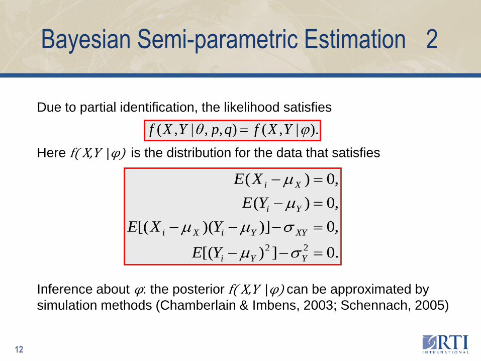
Due to partial identification, the likelihood satisfies

Here f( X,Y |φ) is the distribution for the data that satisfies

Inference about φ: the posterior f( X,Y |φ) can be approximated by

simulation methods (Chamberlain & Imbens, 2003; Schennach, 2005)

12

).|,(),,|,( YXfqpYXf

.0])[(

,0)])([(

,0)(

,0)(

22

YYi

XYYiXi

Yi

Xi

YE

YXE

YE

XE


Inference about structural parameters, for example β :

The data are informative about φ. Beliefs about β are updated

through the conditional prior.

In a partially identified model the prior always retains influence,

even asymptotically.

13

).|(),|(

)|()]()|,([

)()|(),|,(),|,(

fYXf

ffYXf

ffYXfYXf

Application 1

Data: public use file of the 2009 National Survey on Drug Use

and Health (NSDUH)

X : indicator of lifetime/past month/past year drug abstinence

Y : annual family income (in $1,000s)

14

most

recent

use

cocaine crack hallucinogens painkillers stimulants

lifetime 12.0% 2.9% 14.0% 16.7% 7.3%

past year 2.7% 0.4% 3.7% 7.8% 1.9%

past month 0.8% 0.2% 1.0% 3.3% 0.7%

Application 2

Focus on past year use of painkillers. Recall the parameter of

interest:

Assume some degree of under-reporting (p ≥ 0) but no over-

reporting (q = 0).

Bounds for p and β :

15

.26.292ˆ,60.6ˆ

,)1(

92.0ˆ),1(0

2

22

2

UL

XY

YX

X

XYX

X

XY

UXYXU ppp

,

)0|()1|( ZYEZYE

Application 3

Potential prior distributions:

16

).,()|(

1.0),0(

1.0),1.0(1.0)1.0,0(9.0)|(

),,0()|(

3

2

1

UL

UU

UU

U

Uf

ppU

ppUUpf

pUpf

if

if

Application 3

17

Posterior distribution of (p, β, π), using prior f1(p | φ)

Highest posterior density interval (95%)

parameter lower limit upper limit

β 4.94 15.66

π 0.40 0.92

Application 4

Posterior distribution of (p, β, π), using prior f2(p | φ)


18


β 5.18 8.15

π 0.84 0.92

Application 5

Posterior distribution of (p, β, π), using prior f3(β | φ)


19


β 6.97 285.58

π 0.01 0.30

Conclusion

Bayesian inference is an attractive option in partially identified

models;

Nonparametric parameter bounds can be derived, but may be

uninformative in practice;

Prior information, incorporated in a probabilistic (rather than

deterministic) manner, can sharpen inference;

In models with unidentified parameters the prior remains

influential, even asymptotically. It is therefore important to

carefully investigate the implications of any prior.

20

References 1

Biemer, P.P. & Wiesen, C. (2002). Measurement error evaluation of self-reported drug use: a latent class analysis of the

National Household Survey on Drug Abuse. Journal of the Royal Statistical Society A 165, 97-119.

Boese, D.H., Young, D.M. & Stamey, J.D. (2006). Confidence intervals for a binomial parameter based on binary data

subject to false-positive misclassification. Computational Statistics and Data Analysis 50, 3369-3385.

Bollinger, C.R. (1996). Bounding Mean Regressions When a Binary Regressor is Mismeasured. Journal of

Econometrics 73, 387-399.

Bollinger, C.R. (2001). Measurement Error and the Union Wage Differential. Southern Economic Journal 68, 60-78.

Bollinger, C.R. & David, M.H. (1997). Modeling Discrete Choice with Response Error: Food Stamp Participation. Journal

of the American Statistical Association 92, 827-835.

Chamberlain, G. & Imbens, G.W. (2003). Nonparametric applications of Bayesian inference. Journal of Business and

Economic Statistics 21, 12-18.

Del Boca, F.K. & Darkes, J. (2003). The validity of self-reports of alcohol consumption: state of the science and

challenges for research. Addiction 98 (Suppl. 2), 1-12.

Dellaportas, P. & Stephens, D.A. (1995). Bayesian Analysis of Errors-in-Variables Regression Models. Biometrics 51,

1085-1095.

Gustafson, P. (2004). Measurement error and misclassification in statistics and epidemiology: impacts and Bayesian

adjustments. CRC Press.

Joseph, L., Gyorkos, T.W. & Coupal, L. (1995). Bayesian Estimation of Disease Prevalence and the Parameters of

Diagnostic Tests in the Absence of a Gold Standard. American Journal of Epidemiology 141, 263-272

21

References 2

Kroutil, L.A., Vorburger, M., Aldworth, J. & Colliver, J.D. (2010). Estimated drug use based on direct questioning and

open-ended questions: responses in the 2006 National Survey on Drug Use and Health. International Journal of

Methods in Psychiatric Research 19, 74-87.

Kuha, J. (1997). Estimation by Data-Augmentation in Regression Models with Continuous and Discrete Covariates.

Statistics in Medicine 16, 189-201.

Rahme, E., Joseph, L. & Gyorkos, T.W. (2000). Bayesian sample size determination for estimating binomial parameters

from data subject to misclassification. Applied Statistics 49, 119-128.

Schennach, S.M. (2005). Bayesian Exponentially Tilted Empirical Likelihood. Biometrika 92, 31-46.

Swartz, T., Haitovsky, Vexler, A. & Yang, T. (2004). Bayesian identifiability and misclassification in multinomial data.

Canadian Journal of Statistics 32, 285-302.

22

classification errors in regression models: a … international is a trade name of research triangle...

Documents