classification - classification: logistic regression

Motivation Hypothesis Decision boundary Parameter fitting and cost function

ClassificationClassification: logistic regression

Huiping Cao

Huiping Cao, Slide 1/21


Outline

1 Motivation

2 Hypothesis

3 Decision boundary

4 Parameter fitting and cost function



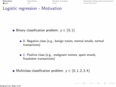
Logistic regression - Motivation

Binary classification problem: y ∈ {0, 1}

0: Negative class (e.g., benign tutors, normal emails, normaltransactions)

1: Positive class (e.g., malignant tumors, spam emails,fraudulent transactions)

Multiclass classification problem: y ∈ {0, 1, 2, 3, 4}



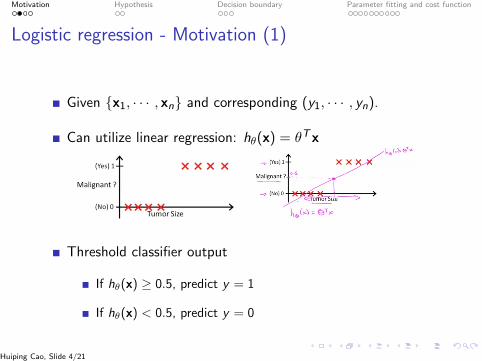
Logistic regression - Motivation (1)

Given {x1, · · · , xn} and corresponding (y1, · · · , yn).

Can utilize linear regression: hθ(x) = θTx

Threshold classifier output

If hθ(x) ≥ 0.5, predict y = 1

If hθ(x) < 0.5, predict y = 0




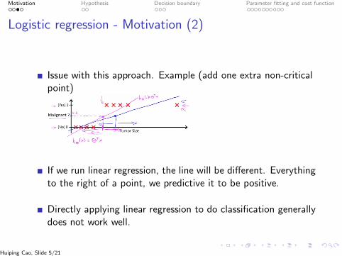
Issue with this approach. Example (add one extra non-criticalpoint)

If we run linear regression, the line will be different. Everythingto the right of a point, we predictive it to be positive.

Directly applying linear regression to do classification generallydoes not work well.




For classification problem, the labels y = 0 or y = 1

If we use linear regression, hθ(x) can be > 1 or < 0.This is very different from the class labels.

Logistic regression: 0 ≤ hθ(x) ≤ 1 to conduct classification.

Logistic regression problem: output is bounded real number.probability ∈ [0, 1].



Logistic regression - Hypothesis (1)

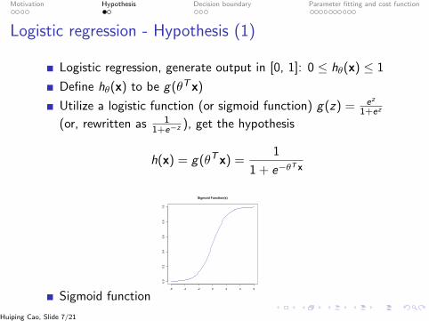
Logistic regression, generate output in [0, 1]: 0 ≤ hθ(x) ≤ 1

Define hθ(x) to be g(θTx)

Utilize a logistic function (or sigmoid function) g(z) = ez

1+ez

(or, rewritten as 11+e−z ), get the hypothesis

h(x) = g(θTx) =1

1 + e−θT x

Sigmoid function-6 -4 -2 0 2 4 6

0.0

0.2

0.4

0.6

0.8

1.0

Sigmoid Function(s)



Logistic regression - Hypothesis (2)

Interpretation of hypothesis output

hθ(x): for the input x, the estimated probability that y = 1.

ExampleIf

x =

(x·0x·1

)=

(1

tumor size

)hθ(x) = 0.7 tells that 70% chance the tumor is malignant.

hθ(x) = P(y = 1|x; θ)Probability that y = 1 given x, parameterized by θ.

P(y = 0|x; θ) + P(y = 1|x; θ) =1P(y = 0|x; θ) = 1- P(y = 1|x; θ)



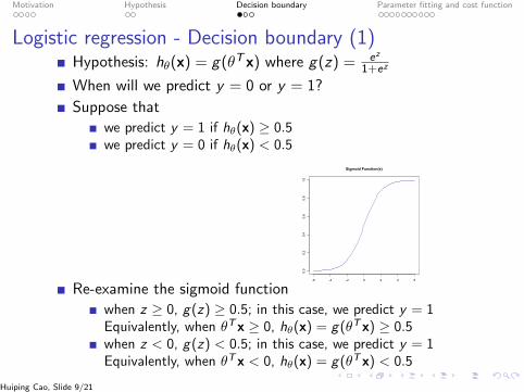
Logistic regression - Decision boundary (1)Hypothesis: hθ(x) = g(θTx) where g(z) = ez

1+ez

When will we predict y = 0 or y = 1?

Suppose that

we predict y = 1 if hθ(x) ≥ 0.5we predict y = 0 if hθ(x) < 0.5

Re-examine the sigmoid function-6 -4 -2 0 2 4 6

0.0

0.2

0.4

0.6

0.8

1.0

Sigmoid Function(s)

when z ≥ 0, g(z) ≥ 0.5; in this case, we predict y = 1Equivalently, when θTx ≥ 0, hθ(x) = g(θTx) ≥ 0.5when z < 0, g(z) < 0.5; in this case, we predict y = 1Equivalently, when θTx < 0, hθ(x) = g(θTx) < 0.5



Logistic regression - Decision boundary (2)

0 1 2 3 4

01

23

4

x1

x2

0 1 2 3 4

01

23

4

●●

●

●

●

●

●

●

●●

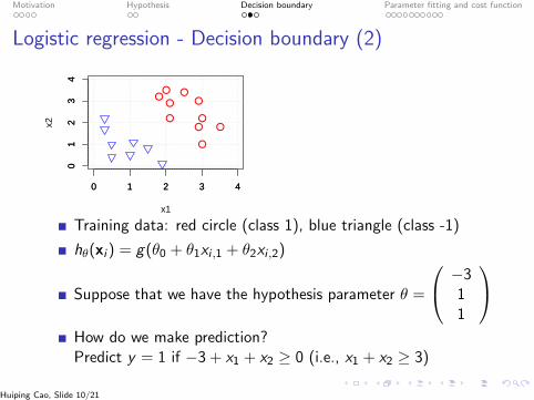
Training data: red circle (class 1), blue triangle (class -1)

hθ(xi ) = g(θ0 + θ1xi ,1 + θ2xi ,2)

Suppose that we have the hypothesis parameter θ =

−311

How do we make prediction?Predict y = 1 if −3 + x1 + x2 ≥ 0 (i.e., x1 + x2 ≥ 3)



Logistic regression - Decision boundary (3)

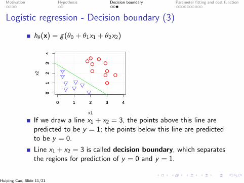
hθ(x) = g(θ0 + θ1x1 + θ2x2)

0 1 2 3 4

01

23

4

x1

x2

0 1 2 3 4

01

23

4

●●

●

●

●

●

●

●

●●

If we draw a line x1 + x2 = 3, the points above this line arepredicted to be y = 1; the points below this line are predictedto be y = 0.

Line x1 + x2 = 3 is called decision boundary, which separatesthe regions for prediction of y = 0 and y = 1.



Logistic regression - Fit the parameters θ (1)

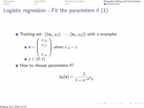
Training set: {(x1, y1), · · · , (xn, yn)} with n examples

x =

x·,0x·,1· · ·x·,d

where x·,0 = 1

y ∈ {0, 1}How to choose parameters θ?

hθ(x) =1

1 + e−θT x



Logistic regression - Fit the parameters θ (2)

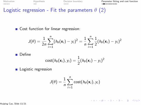
Cost function for linear regression:

J(θ) =1

2n

n∑i=1

(hθ(xi )− yi )2 =

1

n

n∑i=1

1

2(hθ(xi )− yi )

2

Define

cost(hθ(xi ), yi ) =1

2(hθ(xi )− yi )

2

Logistic regression

J(θ) =1

n

n∑i=1

cost(hθ(xi ), yi )



Logistic regression - Cost function (1)

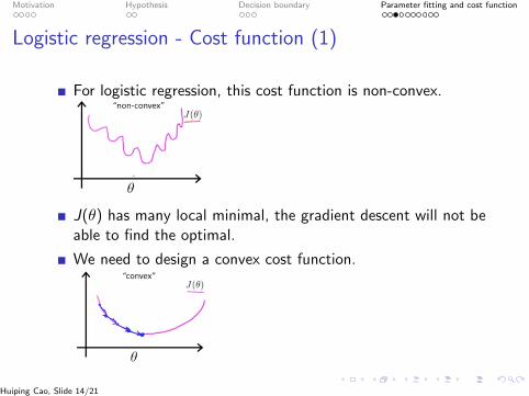
For logistic regression, this cost function is non-convex.

J(θ) has many local minimal, the gradient descent will not beable to find the optimal.

We need to design a convex cost function.



Logistic regression - log function

cost(hθ(x), y) =

{−log(hθ(x)) if y=1−log(1− hθ(x)) if y=0

0 2 4 6 8 10

−2

−1

01

2

x

func

tion(

x) (

log(

x))

0 2 4 6 8 10

−2

−1

01

2

x

func

tion(

x) (

−lo

g(x)

)

0.0 0.2 0.4 0.6 0.8 1.0

01

23

4

h(x)

cost

log(x) −log(x) −log(hθ(x))

0.0 0.2 0.4 0.6 0.8 1.0

−4

−3

−2

−1

0

x

func

tion(

x) (

log(

1 −

x))

0.0 0.2 0.4 0.6 0.8 1.0

01

23

4

x

func

tion(

x) (

−lo

g(1

− x

))

0.0 0.2 0.4 0.6 0.8 1.0

01

23

4

h(x)

cost

log(1-x) -log(1-x) −log(1 − hθ(x))




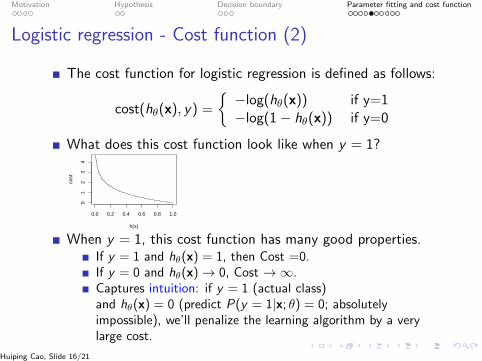
The cost function for logistic regression is defined as follows:

cost(hθ(x), y) =


What does this cost function look like when y = 1?

0.0 0.2 0.4 0.6 0.8 1.0

01

23

4

h(x)

cost

When y = 1, this cost function has many good properties.If y = 1 and hθ(x) = 1, then Cost =0.If y = 0 and hθ(x)→ 0, Cost →∞.Captures intuition: if y = 1 (actual class)and hθ(x) = 0 (predict P(y = 1|x; θ) = 0; absolutelyimpossible), we’ll penalize the learning algorithm by a verylarge cost.




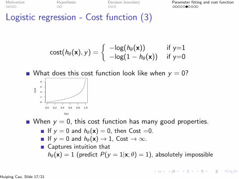
cost(hθ(x), y) =


What does this cost function look like when y = 0?

0.0 0.2 0.4 0.6 0.8 1.0

01

23

4

h(x)

cost

When y = 0, this cost function has many good properties.

If y = 0 and hθ(x) = 0, then Cost =0.If y = 0 and hθ(x)→ 1, Cost →∞.Captures intuition thathθ(x) = 1 (predict P(y = 1|x; θ) = 1), absolutely impossible



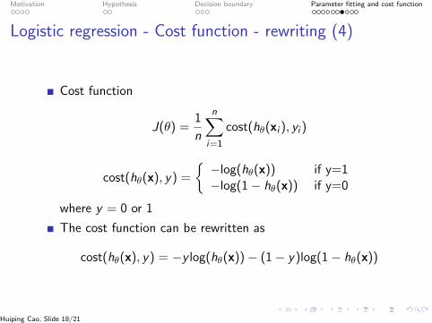
Logistic regression - Cost function - rewriting (4)

Cost function

J(θ) =1

n

n∑i=1

cost(hθ(xi ), yi )

cost(hθ(x), y) =


where y = 0 or 1

The cost function can be rewritten as

cost(hθ(x), y) = −y log(hθ(x))− (1− y)log(1− hθ(x))



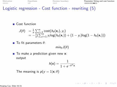
Logistic regression - Cost function - rewriting (5)

Cost function

J(θ) = 1n

∑ni=1 cost(hθ(xi ), yi )

= − 1n (∑n

i=1 yi log(hθ(xi )) + (1− yi )log(1− hθ(xi )))

To fit parameters θ:minθJ(θ)

To make a prediction given new x:output

h(x) =1

1 + e−θT x

The meaning is p(y = 1|x; θ)



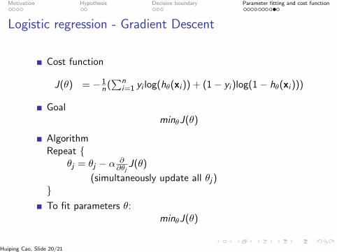
Logistic regression - Gradient Descent

Cost function

J(θ) = − 1n (∑n

i=1 yi log(hθ(xi )) + (1− yi )log(1− hθ(xi )))

GoalminθJ(θ)

AlgorithmRepeat {

θj = θj − α ∂∂θj

J(θ)

(simultaneously update all θj)}To fit parameters θ:

minθJ(θ)



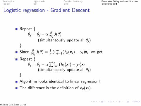
Logistic regression - Gradient Descent

Repeat {θj = θj − α ∂

∂θjJ(θ)

(simultaneously update all θj)}Since ∂

∂θjJ(θ) = 1

n

∑ni=1(hθ(xi )− yi )xi , we get

Repeat {θj = θj − α

∑ni=1(hθ(xi )− yi )xi

(simultaneously update all θj)}Algorithm looks identical to linear regression!

The difference is the definition of hθ(xi ).



R - logistic regression

glm {stats}

R> help(glm) # see several examples.


classification - classification: logistic regression

Documents