robust recognition using l1-principal component analysis
TRANSCRIPT

Rochester Institute of Technology Rochester Institute of Technology
RIT Scholar Works RIT Scholar Works
Theses
4-2015
Robust Recognition using L1-Principal Component Analysis Robust Recognition using L1-Principal Component Analysis
Matthew Johnson
Follow this and additional works at: https://scholarworks.rit.edu/theses
Recommended Citation Recommended Citation Johnson, Matthew, "Robust Recognition using L1-Principal Component Analysis" (2015). Thesis. Rochester Institute of Technology. Accessed from
This Thesis is brought to you for free and open access by RIT Scholar Works. It has been accepted for inclusion in Theses by an authorized administrator of RIT Scholar Works. For more information, please contact [email protected].

Robust Recognition using L1-Principal Component Analysis
by
Matthew Johnson
A Thesis Submitted in Partial Fulfillment of the Requirements for the Degree of
Master of Science in Computer Engineering
Supervised by
Dr. Andreas Savakis
Department of Computer Engineering
Kate Gleason College of Engineering
Rochester Institute of Technology
Rochester, NY
April 2015
Approved By:
_____________________________________________________________________________
Dr. Andreas Savakis
Primary Advisor – R.I.T. Department of Computer Engineering
_____________________________________________________________________________
Dr. Sonia Lopez Alarcon
Committee Member – R.I.T. Department of Computer Engineering
_____________________________________________________________________________
Dr. Raymond Ptucha
Committee Member – R.I.T. Department of Computer Engineering

ii
Dedication
I would like to thank my family, I am forever grateful for your words of encouragement
and unwavering support.

iii
Acknowledgements
I would like to thank my advisor Dr. Andreas Savakis for his assistance and mentorship
in the process of developing this thesis. I would also like to thank my committee
members Dr. Sonia Lopez Alarcon and Dr. Raymond Ptucha. Additionally I want to
thank my colleagues in the Computer Vision Lab Breton Minnehan and Sriram Kumar,
who were invaluable resources throughout this process.

iv
Abstract
The wide availability of visual data via social media and the internet, coupled
with the demands of the security community have led to an increased interest in visual
recognition. Recent research has focused on improving the accuracy of recognition
techniques in environments where variability is well controlled. However, applications
such as identity verification often operate in unconstrained environments. Therefore there
is a need for more robust recognition techniques that can operate on data with
considerable noise.
Many statistical recognition techniques rely on principal component analysis
(PCA). However, PCA suffers from the presence of outliers due to occlusions and noise
often encountered in unconstrained settings. In this thesis we address this problem by
using 𝐿1-PCA to minimize the effect of outliers in data. 𝐿1-PCA is applied to several
statistical recognition techniques including eigenfaces and Grassmannian learning.
Several popular face databases are used to show that 𝐿1-Grassmann manifolds not only
outperform, but are also more robust to noise and occlusions than traditional 𝐿2-
Grassmann manifolds for face and facial expression recognition. Additionally a high
performance GPU implementation of 𝐿1-PCA is developed using CUDA that is several
times faster than CPU implementations.

v
Table of Contents Chapter 1 Introduction ..........................................................................................1
Chapter 2 Background ...........................................................................................4
2.1. Principal Component Analysis .............................................................. 4
2.1.1 L2-PCA ............................................................................................... 4
2.1.2 L1-PCA ............................................................................................... 7
2.2. PCA Recognition ................................................................................. 10
2.3. Grassmannian Recognition .................................................................. 13
2.4. LBP/LTP Features ............................................................................... 16
2.5. GPU Acceleration ................................................................................ 18
2.5.1 General Purpose GPU Computing .................................................... 18
2.5.2 GPU accelerated L1-PCA ................................................................. 21
Chapter 3 L1-PCA Recognition ..........................................................................22
3.1. L1-PCA Algorithm Design .................................................................. 22
3.2. Recognition Techniques ...................................................................... 24
3.2.1 L1-Eigenfaces.................................................................................... 24
3.2.2 L1-Grassmann ................................................................................... 26
3.2.3 LTP Features ..................................................................................... 27
3.3. CPU Implementation ........................................................................... 28
3.4. GPU Implementation ........................................................................... 31

vi
Chapter 4 Experimental Results ..........................................................................36
4.1. Experimental Setup.............................................................................. 36
4.2. Datasets ................................................................................................ 36
4.2.1 Yale Face Database ........................................................................... 36
4.2.2 AT&T Database of Faces .................................................................. 38
4.2.3 Extended Yale Face Database B ....................................................... 39
4.2.4 AR Face Database ............................................................................. 40
4.2.5 Labeled Faces in the Wild Database ................................................. 41
4.2.6 Cohn-Kanade Databases ................................................................... 42
4.3. Parameter Selection ............................................................................. 43
4.4. Accuracy Tests .................................................................................... 44
4.5. Accuracy State of the Art .................................................................... 61
4.5.1 Yale Face Database ........................................................................... 62
4.5.2 AT&T Database of Faces .................................................................. 63
4.5.3 Extended Yale Face Database B ....................................................... 63
4.5.4 AR Face Database ............................................................................. 64
4.6. Speed tests ........................................................................................... 65
Chapter 5 Conclusion and Future Work ..............................................................69
Bibliography ..........................................................................................................72

vii
List of Figures
Figure 1: Multivariate Gaussian with Two Principal Components ........................ 4
Figure 2: L1-PCA Toy Example ............................................................................. 7
Figure 3: First Ten Eigenpictures ......................................................................... 11
Figure 4: Grassmann Manifold Mapping .............................................................. 13
Figure 5: LBP Operator ........................................................................................ 16
Figure 6: LTP Operator ......................................................................................... 17
Figure 7: CPU Architecture (left) vs GPU Architecture (right) ........................... 18
Figure 8: L1-PCA Algorithm Flow....................................................................... 23
Figure 9: Eigenfaces from Occluded Dataset ....................................................... 24
Figure 10: Rectangular Noise on Yale Dataset ..................................................... 25
Figure 11: Recognition using Grassmann Manifolds ........................................... 27
Figure 12: LTP Preprocessing .............................................................................. 28
Figure 13: CPU Tree Reduction ........................................................................... 30
Figure 14: GPU Kernel Flow ................................................................................ 33
Figure 15: GPU Reduction.................................................................................... 34
Figure 16: Min Reduction Kernel ......................................................................... 35
Figure 17: Yale Face Database Images Across Two Subjects .............................. 37
Figure 18: Yale Face Database Sample Image from each Subject ....................... 37
Figure 19: AT&T Database Images Across Two Subjects ................................... 38
Figure 20: AT&T Database Sample Image from each Subject ............................ 38
Figure 21: Extended Yale Face Database B Images Across Two Subjects .......... 39

viii
Figure 22: Extended Yale Face Database B Sample Image from each Subject ... 39
Figure 23: AR Face Database Sample Image from each Subject ......................... 40
Figure 24: AR Face Database Images Across a Subject ....................................... 41
Figure 25: LFW Face Database Images Across Two Subjects ............................. 41
Figure 26: : LFW Face Database Subjects with at Least 20 Images .................... 42
Figure 27: Emotions from the Extended Cohn-Kanade Database ........................ 42
Figure 28: Eigenface Comparison Test Yale Database ........................................ 45
Figure 29: Eigenface Comparison Test AT&T Database ..................................... 45
Figure 30: Grassmann Comparison Test Yale Database ...................................... 46
Figure 31: Grassmann Comparison Test AT&T Database ................................... 46
Figure 32: Grassmann Comparison Test Extended Yale B Database................... 47
Figure 33: Eigenfaces Comparison Test Occluded Yale Database ...................... 48
Figure 34: Eigenfaces Comparison Test Occluded AT&T Database ................... 48
Figure 35: Grassmann Comparison Test Occluded Yale Database ...................... 49
Figure 36: Grassmann Comparison Test Occluded AT&T Database ................... 49
Figure 37: Grassmann Comparison Test Occluded Extended Yale...................... 50
Figure 38: LTP L2-Eigenface t Test for Yale Database ....................................... 51
Figure 39: LTP L1-Eigenface t Test for Yale Database ....................................... 51
Figure 40: LTP Eigenfaces Test Yale Database (t = 2) ........................................ 52
Figure 41: LTP Eigenfaces Test AT&T Database (t = 6) ..................................... 53
Figure 42: LTP Eigenfaces Test Extended Yale B Database (t = 1) .................... 53
Figure 43: LTP Grassmann Test Yale Database (t = 5) ........................................ 54
Figure 44: LTP Grassmann Test AT&T Database (t = 6) .................................... 54

ix
Figure 45: LTP Grassmann Test Extended Yale B Database (t = 5) .................... 55
Figure 46: LTP Grassmann Yale Database (t = 5) ................................................ 57
Figure 47: LTP Grassmann AT&T Database (t = 6) ............................................ 57
Figure 48: LTP Grassmann Extended Yale B Database (t = 5) ............................ 58
Figure 49: LTP Grassmann AR Database (t = 5) .................................................. 58
Figure 50: LTP Grassmann LFW Database (t = 5) ............................................... 59
Figure 51: LTP Grassmann Cohn-Kanade Database (t = 14) ............................... 59
Figure 52: LTP Grassmann Extended Cohn-Kanade Database (t = 16) ............... 60
Figure 53: LTP Grassmann Comparison on Varying number of Subject Images 61
Figure 54: CPU Timing ........................................................................................ 66
Figure 55: GTX Timing ........................................................................................ 66
Figure 56: Tesla Timing........................................................................................ 67
Figure 57: GTX Speedup ...................................................................................... 67
Figure 58: Tesla Speedup...................................................................................... 68

x
List of Tables
Table 1: Grassmann Distance Metrics .................................................................. 15
Table 2: State of the Art Comparison for Yale Face Database ............................. 62
Table 3: State of the Art Comparison for AT&T Database of Faces .................... 63
Table 4: State of the Art Comparison for Extended Yale B Face Database ......... 64
Table 5: State of the Art Comparison for AR Face Database ............................... 64

xi
Glossary
CPU Central Processing Unit
GPU Graphics Processing Unit
ALU Arithmetic Logic Unit
DRAM Dynamic Random-Access Memory
GPGPU General-purpose Computing on Graphics Processing Units
SIMD Single Instruction Multiple Data
SM Streaming Multiprocessors
SP Streaming Processors
CUDA Compute Unified Device Architecture
BLAS Basic Linear Algebra Subprograms
LBP Local Binary Patterns
LTP Local Ternary Patterns

1
Chapter 1 Introduction
Recent research has focused on increasing the accuracy of recognition techniques,
however little effort has been devoted to increasing robustness. Applications such as
surveillance often operate in unconstrained environments where subjects may be partially
occluded by objects such as glasses and scarfs. Thus, there is a significant need for face
recognition techniques that are not only accurate, but also robust to noise.
Many recognition techniques today rely on statistical techniques that perform
direct correlation comparisons between the test face and training databases [1]. To
improve performance many techniques relay on PCA to both reduce dimensionality and
determine better feature subspaces. One of the limitations of PCA is its sensitivity to
outliers, as the 𝐿2-norm has the tendency to exaggerate the influence of noise over valid
data. 𝐿1-PCA utilizes the 𝐿1-norm and as a result is more robust to noise. However, there
is no direct solution for 𝐿1-PCA and iterative solutions must contend with the non-linear
search space. As a result of these limitations, researchers have focused on using
suboptimal solutions to speedup 𝐿1-PCA.
Although suboptimal solutions have improved the speed of 𝐿1-PCA, CPU
implementations still struggle with large datasets. Recently researchers have begun to
utilize general purpose graphics processing units (GPGPU) to speedup algorithms that are
too computationally intensive for CPU processing alone. The GPUs single instruction
multiple data architecture achieves large speedups when an algorithm has a high degree
of data level parallelism. Some early work has shown that the CUDA architecture shows
potential for 𝐿1-PCA [2].
2
Grassmannian learning is an example of a recognition technique that would
benefit from 𝐿1-PCA. The Grassmann manifold has been investigated for variety of
recognition applications, including object, action and face recognition [3], [4]. This
technique maps data subspaces to points on the manifold using PCA. The Grassmann
manifold’s unique geometric structure promotes high class discrimination and
compensates for missing data allowing for great recognition accuracy. However, the
PCA mapping used for Grassmann manifolds is sensitive to outliers and could be
improved with 𝐿1-PCA.
The contributions of this thesis are the following. The first contribution is an
extension of an efficient 𝐿1 principal component algorithm to multiple components that
demonstrates a high degree of robustness to noise. The second contribution is a 𝐿1-PCA
mapping for Grassmann manifolds that can improve accuracy and reduce the effects of
noise in both face and facial expression recognition. The third contribution is an
extension of 𝐿1-Grassmann using local ternary patterns which improves robustness to
variations of illuminations. The final contribution is a high performance implementation
of the 𝐿1-PCA on a GPU using CUDA. This GPU implementation is suitable for
recognition on databases that CPU implementations would not be able to run in a
reasonable amount of time.
This document is organized as follows: Chapter 2 discusses the prior work done
in 𝐿1-PCA and the recognition algorithms used throughout the thesis. Chapter 3 discusses
the how to accelerate proposed 𝐿1-PCA algorithm and details the 𝐿1 versions of the face
and facial expression recognition algorithms. Chapter 4 details the experiments
performed to benchmark the proposed 𝐿1-PCA algorithm as well as the results of the face

3
and facial expression recognition algorithms. Chapter 5 provides a conclusion as well as
potential areas for future work.

4
Chapter 2 Background
This chapter outlines related work in recognition, 𝐿1-PCA and high performance
implementations of 𝐿1-PCA. In Section 2.1 the formulation for 𝐿2-PCA is presented and
the previous work on 𝐿1-PCA is discussed. Previous work in recognition is discussed in
Sections 2.2, 2.3 and 2.4. In section 2.5 GPGPU and how others have leveraged the GPU
for accelerating 𝐿1-PCA algorithms is discussed.
2.1. Principal Component Analysis
2.1.1 L2-PCA
Figure 1: Multivariate Gaussian with Two Principal Components
Principal component analysis was first introduced by Karl Pearson in 1901 and
has been used in a variety of fields including signal processing, pattern recognition and
computer vision [5]. The goal of principal component analysis is to find a set of M
orthogonal vectors aligned in the directions of maximum variance of the data such that
𝑀 ≤ 𝐷, where D is the dimensionality of the data. Figure 1 shows the first two principal
components from a multivariate normal distribution. This process often reveals the

5
underlying structure of data and allows complex datasets to be represented in a lower
dimensionality.
This set of orthogonal vectors are known as eigenvectors or principal components
and can be represented as the matrix 𝑅 ∈ ℜ𝐷×𝑀 where each column is a principal
component aligned with the direction of maximum variance.
Traditional PCA utilizes the 𝐿2-norm which is defined as
𝑑𝐿2 = ‖𝐯‖2 = √ ∑ 𝐯𝑖2
𝑛−1
𝑖=0
(2.1)
where 𝒗 ∈ ℜ𝑛×1. One way to solve for 𝐿2 principal components is by finding the set of
vectors 𝑅 ∈ ℜ𝐷×𝑀 that minimize the 𝐿2-distance between the original signal and its
reconstruction
𝐸2(𝑅, 𝑉) = arg 𝑚𝑖𝑛 ‖𝑋 − 𝑅𝑉‖2 (2.2)
where data matrix 𝑋 ∈ 𝑅𝐷×𝑁, whose columns are data samples such that there are N data
samples and 𝑉 ∈ ℜ𝑀×𝑁 is the coefficient matrix given by
𝑉 = 𝑅𝑇𝑋 (2.3)
without loss of generality, we can assume X is centered such that the set of samples
{𝑥𝑖}𝑖=1𝑁 has zero mean. Using the projection theorem (2.2) can be rewritten as the
following optimization problem
𝑅𝐿2= arg 𝑚𝑖𝑛 ‖𝑋 − 𝑅𝑅𝑇𝑋‖2 (2.4)
Traditionally (2.2) is solved by performing eigen-decomposition on the
covariance matrix of X. The covariance matrix describes the relationships between pairs
of measurements in a dataset [6]. The diagonal elements are the variances across features
6
and the off diagonal elements are the covariance between features. The covariance matrix
is given by
𝑆𝑋 =
1
𝑛 − 1𝑋𝑋𝑇
(2.5)
The PCA process minimizes the square error of the reconstruction, and this is equivalent
to maximizing the captured variance [6]. Eigendecomposition finds a set of orthonormal
vectors that diagonalize the covariance matrix. A single principal component can be
solved using the characteristic equation
𝑆𝑋𝑟𝐿2= 𝜆𝑟𝐿2
(2.6)
where 𝜆 is the eigenvalue corresponding to eigenvector 𝑟𝐿2. Since the covariance matrix
is symmetric it can be decomposed to
𝑆𝑋 = 𝑅𝐿2Σ2𝑅𝐿2
𝑇 (2.7)
where Σ2 is a diagonal matrix containing the variance of each eigenvector in 𝑅𝐿2.
Another way to solve for the principal components is to maximize the trace of Σ2 from
(2.7). This in turn maximizes the variance along the diagonal and solves for the
eigenvectors thus it can be rewritten as
𝑅𝐿2= 𝑎𝑟𝑔𝑚𝑎𝑥 𝑇𝑟𝑎𝑐𝑒(𝑅𝑇𝑆𝑋𝑅) (2.8)
since ‖𝐴‖22 = 𝑇𝑟𝑎𝑐𝑒(𝐴𝑇𝐴) [7], (2.8) can be rewritten into its final form
𝑅𝐿2= 𝑎𝑟𝑔 𝑚𝑎𝑥 ‖𝑋𝑇𝑅‖2 (2.9)
This reformulation is known as the projection energy maximization. Equations (2.2),
(2.4) and (2.9) are 𝐿2 equivalent optimization problems [7].

7
2.1.2 L1-PCA
In 𝐿1-PCA we find a set of orthogonal vectors that are aligned in the direction of
maximum variance with respect to the 𝐿1-norm. The 𝐿1-norm of vector 𝒗 is given by
𝑑𝐿1 = ‖𝒗‖1 = ∑|𝒗𝑖|
𝑛−1
𝑖=0
(2.10)
The main advantage of the 𝐿1-norm is its robustness to outliers. In 𝐿2-PCA outliers with
a large norm are exaggerated by the use of the 𝐿2-norm [8]. Figure 2 highlights the effect
of outliers on 𝐿2-PCA in a toy scenario.
Figure 2: L1-PCA Toy Example
Outliers (left side), L2-PCA (dotted line) and L1-PCA (solid line)
A multivariate Gaussian was used to generate test points and then four of those points
had noise added to them. Both 𝐿2-PCA and 𝐿1-PCA were used to find the first principal

8
component of the data. As shown in Figure 2, 𝐿2-PCA was heavily influenced by the
outliers, while 𝐿1-PCA offered a more accurate representation of the data. The three
equivalent 𝐿2 optimization problems (2.2), (2.4) and (2.9) can be translated to the 𝐿1-
norm and used to solve for the 𝐿1-principal components [7].
𝐸1(𝑅, 𝑉) = arg 𝑚𝑖𝑛 |𝑋 − 𝑅𝑉|1 (2.11)
𝑅𝐿1= arg 𝑚𝑖𝑛 |𝑋 − 𝑅𝑅𝑇𝑋|1 (2.12)
𝑅𝐿1= 𝑎𝑟𝑔 𝑚𝑎𝑥 |𝑋𝑇𝑅|1 (2.13)
Under the 𝐿1-norm the above optimization problems are no longer equivalent because the
PCA scalability property does not hold due to the loss of the projection theorem [9].
In [10], Ke et al. use the error minimization in (2.11) to solve for the 𝐿1 principal
components. Ke et al. solves this problem by utilizing alternating convex minimization.
The 𝐿1-norm cost function in (2. 11) is not generally convex, however if R or V is known
then the problem becomes convex [10]. Utilizing this scheme Ke et al. optimizes (2. 11)
by alternating between optimizing R and V using convex minimization.
Several researchers have explored using the 𝐿1 projection energy optimization in
(2.13) for 𝐿1-PCA. In [8], Kwak introduced a suboptimal approach called PCA-𝐿1 that
iteratively solves the energy maximization problem. Kwak’s algorithm solves for a single
eigenvector by using the optimal polarity to iteratively converge to a vector that
maximizes the 𝐿1 projection energy. The remaining eigenvectors are solved for in a
greedy manner by removing the previous eigenvectors contribution from each data
sample as follows
𝑥𝑖(𝑢𝑝𝑑𝑎𝑡𝑒) = 𝑥𝑖 − 𝑟𝐿1
(𝑟𝐿1𝑇𝑥𝑖) ∀𝑖 ∈ {1, … , 𝑁} (2.14)

9
Kwak’s greedy search algorithm does not guarantee an optimal solution, however it does
guarantee the othronormality of all principal components and that the set of principal
components will maximize 𝐿1 dispersion [8]. The computational complexity of 𝐿1-PCA
with greedy search is 𝑂(𝑀𝑁𝐷𝑇) where T is the number of iterations to converge. The
main issue with Kwak’s solution is that the computational complexity is dependent on the
dimensionality of the data which is equivalent to the number of pixels in an image for
face recognition. In [11], Nie et al. replaced the greedy search method introduced by
Kwak with a non-greedy method. Kwak’s PCA-𝐿1 algorithm is extended to solve for a
set of 𝐿1 eigenvectors simultaneously. The Nie et al. solution does not guarantee
convergence to an optimal 𝐿1-subspace and has the same time complexity as PCA-𝐿1
with greedy search. However Nie et al. has experimentally shown that this non-greedy
approach outperforms the greedy approach on several datasets [11]. In [9], Markopoulos
et al. proves that a single 𝐿1 principal component can be solved for using
𝑟𝐿1
=𝑋𝑏𝑜𝑝𝑡
‖𝑋𝑏𝑜𝑝𝑡‖2
(2.15)
where
𝑏𝑜𝑝𝑡 =
𝑎𝑟𝑔 𝑚𝑎𝑥 ‖𝑋𝑏‖2
𝑏 ∈ {±1}𝑁=
𝑎𝑟𝑔 𝑚𝑎𝑥 𝑏𝑇𝑋𝑇𝑋𝑏
𝑏 ∈ {±1}𝑁
(2.16)
This proof reformulates the 𝐿1 projection energy optimization as a search over a binary
vector. Markopoulos et al. show that the optimal set of 𝐿1 principal components can be
solved by exhaustive searching 2𝑀𝑁 binary matrices of size 𝑁 × 𝑀. Additionally in [9]
Markopoulos et al. show that in the special case 𝑁 ≥ 𝐷 an orthonormal scanning matrix
can be used to solve for an optimal set of 𝐿1 principal components in polynomial time. In

10
subsequent work, Kundu et al. introduced a fast suboptimal method for the computation
of a single 𝐿1-principal component for real-valued data [12]. This algorithm optimizes
(2.16) using greedy bit flipping. The binary vector is optimized by identifying bits that
negatively contribute to the 𝐿1 projection energy and flipping them. The 𝐿1 projection
energy associated with (2.16) can be written as
𝑏𝑇𝑋𝑇𝑋𝑏 = 𝑇𝑟𝑎𝑐𝑒(𝑋𝑇𝑋) + ∑ 2𝑏𝑖 {∑ 𝑏𝑗(𝑋𝑇𝑋)𝑖,𝑗
𝑗>𝑖
}
𝑖
(2.17)
where i and j vary from 1 to N. From (2.17) Kundu et al. [12] show that the contribution
of the ith bit to the aggregative maximum is given by
𝛼𝑖 = ±4𝑏𝑖 ∑ 𝑏𝑗(𝑋𝑇𝑋)𝑖,𝑗
𝑗≠𝑖
(2.18)
This bit flipping is repeated until all bits positively contribute towards the aggregative
maximum or until the maximum number of iterations are reached. This process can be
repeated up to N times using the sign of the columns of the covariance matrix as the
initial values for the binary vectors. The binary vector candidate with the largest
projection energy is determined using (2.16) and the corresponding eigenvector is
obtained from (2.15).
2.2. PCA Recognition
In [13] Kirby et al. showed that principal component analysis could be used to
generate a set of basis features called eigenpictures. In their algorithm they used a set of
face images that was centered such that the eyes of each person were aligned. Next the
images are vectorized to form a column vector with a size equal to the number of pixels

11
in the image. A set of eigenpictures is generated by running principal component analysis
(PCA) on the column vectors as shown in Figure 3. PCA discovers the underlying
Euclidian structure in the data and utilizes that to reduce the dimensionality and hopefully
increase class discrimination. These eigenpictures form a basis and are used to transfer
images to a smaller dimensional feature space. Once in feature space direct correlation
comparisons between the test and training images is used to perform recognition.
Figure 3: First Ten Eigenpictures
In [14] Turk et al. coined the term eigenfaces when they applied Kirby’s et al.
eigenpictures to face recognition. Turk et al. starts of by calculating the eigenfaces using
the same procedure as Kirby et al. The eigenfaces are then sorted using their
corresponding eigenvalues from largest to smallest and a subset is formed using the
eigenvectors with the largest eigenvalues. The larger eigenvalues correspond to
eigenfaces that capture more variance and as a result are better basis vectors. This subset
of eigenvectors is used to transform training and test images into face space using the

12
projection theorem. Once in face space the Euclidean distance between a test image and a
face class is used for recognition. Unfortunately, traditional eigenfaces are not robust to
large variations in illumination, pose, facial expression and the presence of occlusions.
Numerous extensions to eigenfaces have been proposed to overcome its
limitations. Modular eigenfaces is one such extension that is more robust to occlusions,
variations in illumination and facial expression. Modular eigenfaces was first introduced
by Pentland et al in [15]. Pentland et al in divided both eyes, the nose and the mouth into
sub-images and then ran principal component analysis on each sub-image across the
training set [15]. This results in a set of eigenvectors for each sub-image. Similar to
traditional eigenfaces a subset is formed using the eigenvectors with the largest
eigenvalues for each sub-image. The subsets of eigenvectors is used to transform each
sub-image in the training and test images into an alternate space using the projection
theorem. After that the alternate space weights for each sub-image are concatenated into a
single descriptor. Pattern recognition techniques are then applied to these descriptors to
perform face recognition.
The advantage of modular eigenfaces is that by dividing the image areas with
very different illumination or areas with noise wont effect the other sub-images
projection. In [16] Gottumukkal et al. extended Pentland et al. work by dividing the entire
image into sub-images, instead of only using the eyes and mouth images. By dividing the
entire image only a subset of the sub-images would be affected by the variations in
illumination and as a result would be more robust.
In [17], Yang et al. introduced 2D-eigenfaces, another extension to the traditional
eigenfaces technique that improves recognition accuracy and reduces computation time.
13
This technique utilizes 2D-PCA to calculate eigenfaces using the image covariance
matrix. This matrix can more efficiently capture the relationships between images, as
opposed to traditional PCA which needs to vectorize the image before computing the
covariance matrix. Yang et al. demonstrates that 2D-PCA outperforms traditional PCA,
but requires more eigenvectors [17].
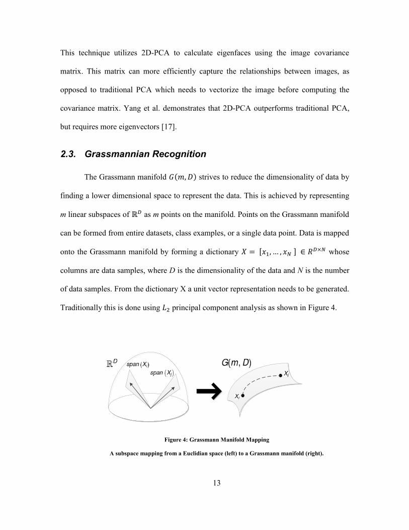
2.3. Grassmannian Recognition
The Grassmann manifold 𝐺(𝑚, 𝐷) strives to reduce the dimensionality of data by
finding a lower dimensional space to represent the data. This is achieved by representing
m linear subspaces of ℝ𝐷 as m points on the manifold. Points on the Grassmann manifold
can be formed from entire datasets, class examples, or a single data point. Data is mapped
onto the Grassmann manifold by forming a dictionary 𝑋 = [𝑥1, … , 𝑥𝑁 ] ∈ 𝑅𝐷×𝑁 whose
columns are data samples, where D is the dimensionality of the data and N is the number
of data samples. From the dictionary X a unit vector representation needs to be generated.
Traditionally this is done using 𝐿2 principal component analysis as shown in Figure 4.
Figure 4: Grassmann Manifold Mapping
A subspace mapping from a Euclidian space (left) to a Grassmann manifold (right).

14
The Grassmann manifold is naturally a smooth curved surface and as a result
Euclidian distance metrics cannot be directly applied. Several different distance metrics
have been explored for Grassmann manifolds based on principal angles between
subspaces 𝜃 = [𝜃1, 𝜃2, … , 𝜃𝑚 ], where the principal angle between two subspaces is given
using SVD such that
𝑥1′𝑥2 = 𝑈𝑆𝑉′ (2.19)
𝑑𝑖𝑎𝑔(𝑆) = (cos 𝜃1 , … , cos 𝜃𝑚) (2.20)
Distance metrics include projection, Binet-Cauchy, max correlation, min correlation,
Procrustes, geodesic and mean distance [3], [18].
In general, metrics that rely on the smallest principal angle tend to be more robust
to noise and less discriminative, while metrics that rely on the largest principal angle tend
to be less robust to noise and more discriminative [19]. The distance between subspaces
can also be calculated by converting the Grassmann manifold to an alternate space using
Grassmann kernel. Projection kernels can be used to create an isometric embedding from
Grassmann space to Hilbert space, which enables the use of Euclidean distance metrics.
From [3], the projection kernel between subspaces 𝑥1, 𝑥2 can be formed using
𝐾𝑝(𝑥1, 𝑥2) = ‖𝑥1′𝑥2‖𝐹
2 (2.21)
where ‖ ‖𝐹 is the Frobenius norm. Projection kernels do not define a direct linear
relationship between subspaces and as a result kernel based methods such as PCA or
LDA are needed for accurate classification [19].
Grassmann manifolds have been investigated for computer vision applications,
such as object, action and face recognition. In [3] Hamm and Lee used Grassmann kernel
LDA to increase performance in face and object recognition. Turaga et al. used

15
probability density functions to estimate classes on the Grassmann manifold in [4] and
applied it to activity recognition, affine shape analysis and video based face recognition.
In [18] Shigenaka et al. introduced GD-MSM and GK-SVM, which use the Grassmann
manifold to improve the performance of mutual subspace method and support vector
machines. In [19] Azary introduced Grassmannian Sparse Representations for 3D action
and face recognition.
Table 1: Grassmann Distance Metrics
Metric Name Metric Equation
Projection
𝑑𝑝(𝑥1, 𝑥2) = (𝑚 − ∑ cos2 𝜃𝑖
𝑚
𝑖=1
)
12
(2.22)
Binet-Cauchy
𝑑𝑝(𝑥1, 𝑥2) = (1 − ∏ cos2 𝜃𝑖𝑖
)
12
(2.23)
Max Correlation 𝑑𝑝(𝑥1, 𝑥2) = (1 − cos2 𝜃1)
12
(2.24)
Min Correlation 𝑑𝑝(𝑥1, 𝑥2) = (1 − cos2 𝜃𝑚)
12
(2.25)
Procrustes
𝑑𝑝(𝑥1, 𝑥2) = 2 (∑ sin2𝜃𝑖
2
𝑚
𝑖=1
)
12
(2.26)
Geodesic 𝑑𝑝(𝑥1, 𝑥2) = ∑ 𝜃𝑖
2
𝑚
𝑖=1
(2.27)
Mean Distance 𝑑𝑝(𝑥1, 𝑥2) =
1
𝑚∑ sin2 𝜃𝑖
𝑚
𝑖=1
(2.28)

16
2.4. LBP/LTP Features
Large variations in illumination are a challenging test case for many image based
recognition techniques. One solution is to rely on descriptors based on texture rather than
raw pixels. Local binary patterns (LBP) and local ternary patterns (LTP) summarize local
grey-level structure and as a result are resistant to the effects of illumination. In [20],
Ojala et al. introduced LBP for illumination invariant texture classification. In this
technique a binary code is generated for each pixel in an image by comparing the center
pixel to the neighboring pixels. The binary codes are given by the following
𝐿𝐵𝑃 = ∑ 2𝑖𝑠(𝑦𝑖 − 𝑦𝑐)
𝑛
𝑖=0
(2.29)
where 𝑦𝑐 is the center pixel intensity, 𝑦𝑖 is the pixel intensity in the surrounding
neighborhood and s is given by
𝑠(𝑢) = {
1, 𝑢 ≥ 0 0, 𝑢 < 0
} (2.30)
Originally the neighborhood was defined as the 3 x 3 area around the target pixel,
however other patterns have been explored. Figure 5 highlights the encoding process
using a 3 x 3 image patch.
92 50 26
99 60 70
54 12 60
1 0 0
1 1
0 0 1
Threshold
Binary Code:10011001
Figure 5: LBP Operator

17
LBP is highly discriminative on areas with uniform illumination, however areas with
gradual illumination change introduce noise [21]. Tan et al. eliminate this issue by
introducing LTP in [21], which replaces the threshold with a range and the binary code
with a ternary code. Local ternary codes are given by the following
𝐿𝑇𝑃 = ∑ 3𝑖𝑠′(𝑦𝑖 − 𝑦𝑐 , 𝑦𝑐, 𝑡 )
𝑛
𝑖=0
(2.31)
where t is a user specified threshold and s’ is given by
𝑠′(𝑢, 𝑦𝑐 , 𝑡) = {
1, 𝑢 ≥ 𝑦𝑐 + 𝑡0, 𝑦𝑐 − 𝑡 < 𝑢 < 𝑦𝑐 + 𝑡
−1, 𝑢 ≤ 𝑦𝑐 − 𝑡}
(2.32)
92 50 26
99 60 70
54 12 60
1 -1 -1
1 1
0 -1 0
Threshold
Ternary Code:1(-1)(-1)10(-1)01
t=10
1 0 0
1 1
0 0 0
0 1 1
0 0
0 1 0
Binary Code:01100100
Binary Code:10010001
1's Pattern
-1's Pattern
Figure 6: LTP Operator
For simplicity the ternary code is split into two binary codes and processed separately.
Figure 6 shows this process for a 3 x 3 image patch. To perform recognition LBP/LTP is
run on an image and local histograms are generated for image subsections. These

18
histograms are then concatenated to form a descriptor and recognition is performed using
pattern recognition techniques.
2.5. GPU Acceleration
2.5.1 General Purpose GPU Computing
Originally GPUs were designed to reduce the computational load of the CPU by
solely processing graphics request. In order to optimize graphics operations GPUs utilize
a single instruction multiple data (SIMD) architecture, which simplifies control logic and
utilizes a large number of simple arithmetic logic units (ALU) to take advantage of data
level parallelism as shown in Figure 7.
In 2007, NVIDIA recognized the potential for heterogeneous CPU/GPU solutions and
released the first general purpose computing on the GPU (GPGPU) API, the Compute
Figure 7: CPU Architecture (left) vs GPU Architecture (right)
DRAM
Cache
Control Unit
ALU ALU
ALU ALU
DRAM
19
Unified Device Architecture (CUDA) [22]. CUDA and other GPGPU APIs have allowed
researchers to speedup algorithms that were previously too computationally intensive for
CPUs alone.
In order to maximize the performance of an algorithm on the GPU, the underlying
hardware must be considered. CUDA-capable GPUs are organized into arrays of
streaming multiprocessors (SM). Each streaming multiprocessor is composed of a set of
streaming processors (SP) and connected to a shared block of DRAM called global
memory. Each streaming processor shares control logic, an instruction cache, registers
and another block of DRAM called shared memory. The number of streaming
multiprocessors and streaming processors is important to consider when developing
CUDA applications because they determine the maximum number of threads that can be
run simultaneously. In CUDA threads are organized into 3D blocks which make up a 3D
grid. The dimensionality of each of these 3D block/3D grid structures is application
dependent. At runtime each streaming multiprocessor is assigned a block from the grid
to execute. Each block is broken into groups of 32 threads called warps prior to
execution. Each warp is then run in a serial manner over the streaming processors, this
allows for fast context switching between warps when a stall is encountered.
Another important hardware consideration is memory usage, CUDA-capable
GPUs allow the use of five different types of memory: registers, shared memory, global
memory, constant memory, and texture memory. The bandwidth of the GPU’s global
memory is often a bottleneck in CUDA programs, therefore proper memory usage is
important when developing high performance applications. Threads store local variables
in registers and any overflow in a private section of global memory called local memory.

20
Registers are the fastest memory on the GPU, therefore it is important to limit the number
of local variables for high performance applications. Shared memory is a read/write
memory that allows memory sharing across threads in the same block. This is achieved
by local DRAM blocks within each streaming multiprocessor. Overall this allows for
much faster data storage without contributing to the global memory bandwidth. Global
memory is a read/write memory that allows memory access by any thread. All incoming
data and outgoing results must pass through global memory and as a result it is often the
main bottleneck of the GPU. Another form of memory is constant memory which only
allows read operations during runtime. Like global memory constant memory can be
accessed by any thread, however it is highly cached making it much quicker than global
memory. The final memory type is texture memory which is a special read only memory
that has been optimized for texture based operations. Using special hardware built into
the pipeline several common texture functions can be performed automatically including
pixel interpolation and border wrapping. Unlike other forms of memory on the GPU,
texture memory has constant access times for both cache hits and misses which allows for
better scheduling and a 2D cache which gives it greater 2D spatial access.
There are several important design constraints to keep in mind when developing
high performance algorithms in CUDA. Block size is very important design constraint in
GPGPU because it controls how well your program hides memory latency. Generally
block sizes are a fraction of the number of threads that a streaming multiprocessor can
support so that multiple blocks can run on one streaming multiprocessor. The number of
threads in a block should be a multiple of 32, to ensure that only full warps are generated.
The number of conditional statements is another important factor to consider in high

21
performance applications. When a conditional branch statement is encountered in CUDA
the diverging threads may need to be stalled until all threads converge. Therefore, to get
good hardware utilization it is important to limit the number of conditional statements. As
a result this reduces hardware utilization. One of the most important keys when working
in CUDA is to be observant of the memory access patterns. In order to reduce overhead
involved with accessing global memory each read has the potential to fetch 64
consecutive bytes. If memory is not coalesced it could take up to 16 reads to fetch the
same number of bytes.
2.5.2 GPU accelerated L1-PCA
There has been a lot of research on how to best utilize GPU resources to speedup
algorithms. However, there has been very little research on how to specifically accelerate
𝐿1-PCA using the GPU. In [2] Funatsu et al. accelerated Kwak’s PCA-𝐿1 algorithm from
[8] using the GPU. Funatsu et al. do not specify which portions of Kwak’s PCA-𝐿1
algorithm they accelerated using the GPU. However, they do utilize CUBLAS, which is
CUDAs optimized BLAS (Basic Linear Algebra Subprograms) library. Funatsu et al.
report speedups between 1.72 – 2.96 over the CPU on small datasets [2].

22
Chapter 3 L1-PCA Recognition
This chapter describes several approaches to recognition based on 𝐿1-PCA. The
design of the 𝐿1-PCA algorithm is discussed in Section 3.1. In Section 3.2 the
implementation of the 𝐿1-Eigenfaces, 𝐿1-Grassmann and LTP preprocessing is outlined.
The CPU implementation of 𝐿1-PCA is specified in Section 3.3. Lastly this chapter
details the 𝐿1-PCA GPU implementation in Section 3.4.
3.1. L1-PCA Algorithm Design
Recent work by Kundu et al. [12] introduced a fast computation for a single 𝐿1
principal component using bit flipping to maximize the 𝐿1 projection energy. The
advantage of the Kundu et al. method is that the complexity is 𝑂(�̃�𝑁2) where N is the
number of samples and �̃� is the number of initializations which are chosen by the user.
Unlike previous solutions this method does not rely on the dimensionality of the data
which makes it ideal for image recognition where the dimensionality is usually the
number of pixels in the image. This method is extended to multiple components using the
greedy search algorithm introduced by Kwak in [8]. Subsequent principal components are
calculated by removing each principal components contribution from the data samples
and utilizing the updated dataset to find the next principal component. This process is
repeated until the desired number of components is reached. The greedy search algorithm
guarantees that the principal components maximize the 𝐿1-dispersion [8]. The overall
algorithm flowchart is shown in Figure 8. The time complexity for the full algorithm is
𝑂(𝑀�̃�𝑁2) where M is the number of principal components.

23
Start
Calculate Covariance
Matrix
Update Data Samples
Increment vectorCount
False
True
EndFalse
Initialize Binary Vector
True
Calculate Binary Vector
Contributions
Increment sampleCount
True
Update Binary Vector
False
Set sampleCount to
zero
vectorCount
sampleCount < # data samples
vectorCount < # eigenvectors
All contributions are Positive
Figure 8: L1-PCA Algorithm Flow

24
3.2. Recognition Techniques
3.2.1 L1-Eigenfaces
Much research has been performed to make eigenfaces more robust to variations
in illumination and expression [23], [24], [25]. Utilizing the 𝐿1-norm instead of the 𝐿2-
norm for eigenfaces allows for more accurate recognition on unconstrained or noisy
datasets. Figure 9 shows the first ten eigenfaces generated from a subset of the aligned
Yale Face database [25].
(a.)
(b.)
Figure 9: Eigenfaces from Occluded Dataset
The first 10 eigenfaces based on (a) L2-PCA and (b) L1-PCA from Yale Face Database.
25
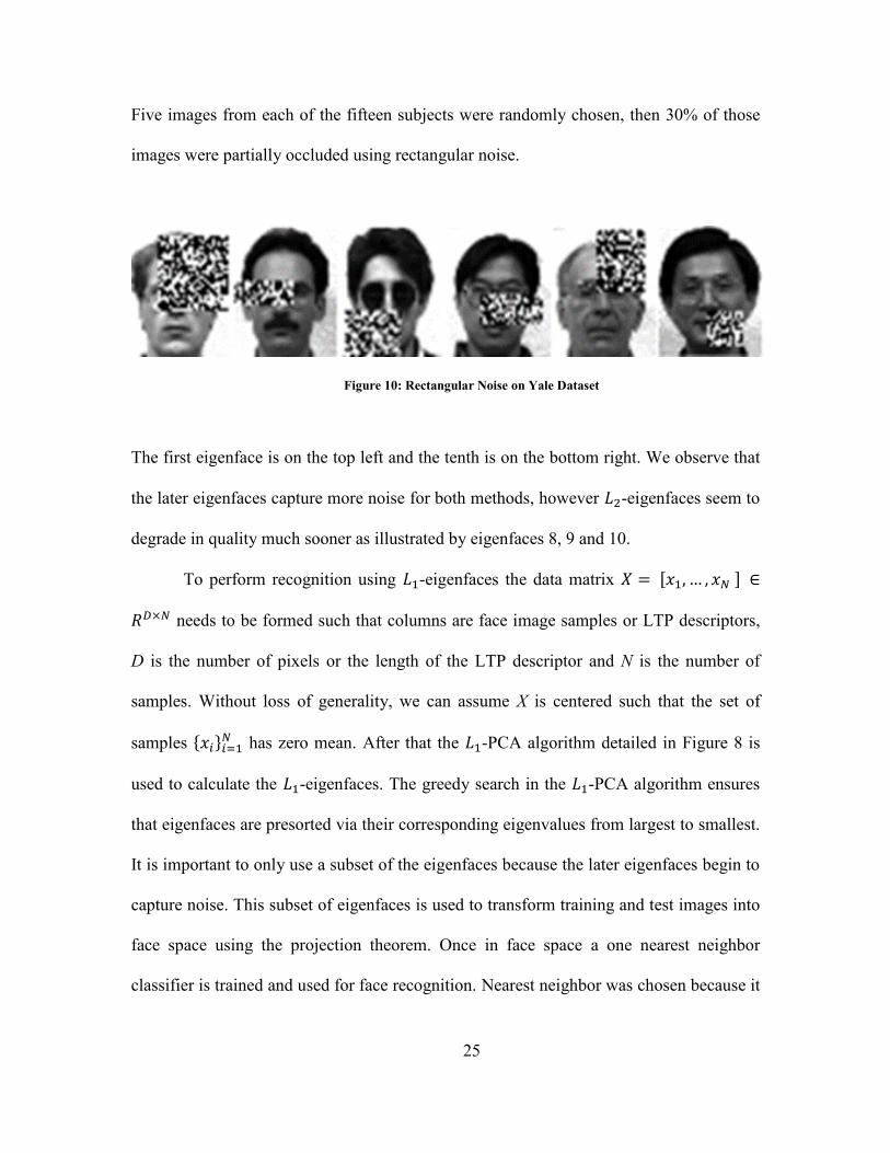
Five images from each of the fifteen subjects were randomly chosen, then 30% of those
images were partially occluded using rectangular noise.
Figure 10: Rectangular Noise on Yale Dataset
The first eigenface is on the top left and the tenth is on the bottom right. We observe that
the later eigenfaces capture more noise for both methods, however 𝐿2-eigenfaces seem to
degrade in quality much sooner as illustrated by eigenfaces 8, 9 and 10.
To perform recognition using 𝐿1-eigenfaces the data matrix 𝑋 = [𝑥1, … , 𝑥𝑁 ] ∈
𝑅𝐷×𝑁 needs to be formed such that columns are face image samples or LTP descriptors,
D is the number of pixels or the length of the LTP descriptor and N is the number of
samples. Without loss of generality, we can assume X is centered such that the set of
samples {𝑥𝑖}𝑖=1𝑁 has zero mean. After that the 𝐿1-PCA algorithm detailed in Figure 8 is
used to calculate the 𝐿1-eigenfaces. The greedy search in the 𝐿1-PCA algorithm ensures
that eigenfaces are presorted via their corresponding eigenvalues from largest to smallest.
It is important to only use a subset of the eigenfaces because the later eigenfaces begin to
capture noise. This subset of eigenfaces is used to transform training and test images into
face space using the projection theorem. Once in face space a one nearest neighbor
classifier is trained and used for face recognition. Nearest neighbor was chosen because it

26
is arguably one of the simplest classifiers and as a result it is better at highlighting the
disparity between methods.
3.2.2 L1-Grassmann
Subspaces on the Grassmann manifold can be formed from a single data point or
multiple data samples. As a result the Grassmann manifold can be used to make single-
single, single-many or a many-many comparisons. To highlight the advantages of 𝐿1-
Grassmann we perform a many-many comparison where each subspace is composed of
data samples from a single class. This doubles the effect of 𝐿1-PCA by allowing it to
reduce the effect of noise on both training and test images.
To construct 𝐿1-Grassmann manifolds, first dictionaries are formed by sorting all
training images or LTP descriptors and grouping them by the person’s identity for face
recognition or by expression for expression recognition. Each element in the dictionary is
obtained by lexicographic ordering of all the image columns or by LTP preprocessing.
Each class subspace is then mapped onto the 𝐿1-Grassmann manifold by using the 𝐿1-
PCA algorithm detailed in Figure 8 to calculate the principle components for each class.
After that the projection kernel is formed for the training and test set, which projects the
manifold onto Hilbert space. Once in Hilbert space Grassmann PCA is used to reduce the
dimensionality of the data and one-nearest neighbor classification is used for recognition.
This entire process is shown below in Figure 11.

27
N
D
q q q
PCA PCA PCA
D
q q q
PCA
1 NN
Figure 11: Recognition using Grassmann Manifolds
3.2.3 LTP Features
Local ternary patterns decode the grayscale structure in images and as a result can
greatly improve accuracy in datasets with large variations in illumination. After
performing LTP on an image traditional methods divide the LTP image into sub-regions
and generate local histograms. These histograms are then concatenated together and used
as a descriptor for the image. This technique reduces the dimensionality of the data by
throwing away the spatial information within sub-regions. Since Eigenfaces and
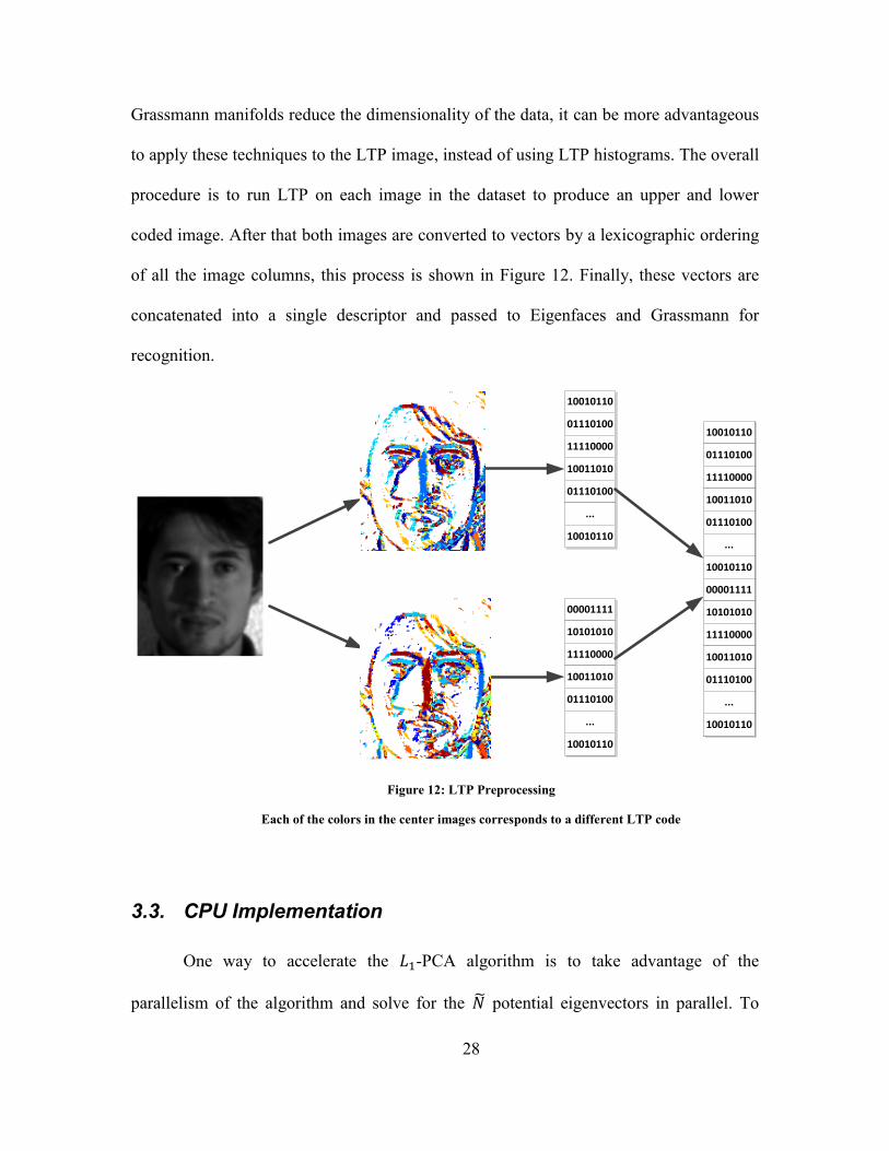
28
Grassmann manifolds reduce the dimensionality of the data, it can be more advantageous
to apply these techniques to the LTP image, instead of using LTP histograms. The overall
procedure is to run LTP on each image in the dataset to produce an upper and lower
coded image. After that both images are converted to vectors by a lexicographic ordering
of all the image columns, this process is shown in Figure 12. Finally, these vectors are
concatenated into a single descriptor and passed to Eigenfaces and Grassmann for
recognition.
10010110
01110100
11110000
10011010
01110100
...
10010110
00001111
10101010
11110000
10011010
01110100
...
10010110
10010110
01110100
11110000
10011010
01110100
10001111
10010110
10010110
01110100
11110000
10011010
01110100
...
10010110
10010110
01110100
11110000
10011010
01110100
...
10010110
00001111
10101010
11110000
10011010
01110100
...
10010110
Figure 12: LTP Preprocessing
Each of the colors in the center images corresponds to a different LTP code
3.3. CPU Implementation
One way to accelerate the 𝐿1-PCA algorithm is to take advantage of the
parallelism of the algorithm and solve for the �̃� potential eigenvectors in parallel. To

29
accomplish this the serial operations are vectorized and rewritten as a series of matrix
operations. With this reformulation the goal becomes to optimize the binary matrix 𝐵 ∈
ℝ�̃�×𝑁 where each row corresponds to a potential eigenvector. The contributions of each
bit in the binary matrix is solved simultaneously using
𝑄 = 𝐵.∗ (𝐵 𝑆𝑋) − 𝐷 (3.1)
where .∗ is element-wise multiplication and 𝐷 ∈ 𝑅�̃�×𝑁 is
𝐷 = [𝑑𝑖𝑎𝑔( 𝑆𝑋)
⋮𝑑𝑖𝑎𝑔( 𝑆𝑋)
]
(3.2)
The binary matrix is updated by finding the minimum value in each row of 𝑄 and
flipping the corresponding bits in the matrix 𝐵. To improve performance all minimum
reductions are performed in parallel. This process is repeated until no bit in B contributes
negatively or until the maximum number of iterations are reached. From the optimized
matrix B the optimal binary vector is calculated by finding the row with the maximum
projection energy. The following equation gives the projection energy for each row
𝐸𝑝 = ∑(𝐵.∗ (𝐵 × 𝑆𝑋)):,𝑖
𝑁
𝑖=0
(3.3)
where 𝐸𝑝 ∈ ℝ�̃�×1. The optimal binary vector is than determine by performing a
maximum reduction on 𝐸𝑝 to find the largest corresponding projection energy. To ensure
the optimal matrix operation performance the Intel Math Kernel Library which utilizes
Basic Linear Algebra Subprograms (BLAS) was used to implement the algorithm for the
CPU.

30
3.3.1.1 Reduction Algorithms
One of the most important areas to accelerate is the min and max reductions
because of the large number of reductions used throughout the algorithm. The goal of a
reduction algorithm is to perform an operation over a data vector and return a single
value. This operation is often associative which allows it to be computed in a partially
parallel manner. There are several reduction algorithms that are utilized throughout the
𝐿1-PCA algorithm including the calculation of the minimum contributing bit and the
calculation of optimal binary vector. To ensure high performance Intel’s
parallel_reduce function from the threading building blocks library was used. To
maximize the parallelism in reduction algorithms this function generates a tree structure
by recursively splitting the data vector into subranges until each subrange is no longer
divisible as shown in Figure 13.
Figure 13: CPU Tree Reduction
A[10, 19]
A[0, 19]
A[0, 9]
A[0, 4] A[5, 9] A[10, 14] A[15, 19]
A = 0 1 2 3 4 5 ... 19
31
Each node performs the desired operation such as max or min over its range and passes
the result to the parent node. After that the parent node repeats this operation on the
resultant of the child nodes. This process repeats until a single result is obtained through
the root. This structure enables nodes at the same depth to be run in parallel and as a
result accelerates the operation.
3.3.1.2 Parallel Operations
Some of the matrix operations such as binary matrix initialization and
optimization can be implemented more efficiently using custom parallel functions instead
of BLAS functions. To ensure optimal performance Intel’s parallel_for function was
used for the custom functions. In a similar manner to the reduction algorithm the data
vectors are recursively split into subranges until each subrange is no longer divisible.
However in this case each subrange is independent and as a result only the leaf nodes
need to be executed. Upon execution each element in a nodes subrange is executed in a
synchronous fashion, however each node is executed in parallel. This methodology
ensures that each thread is performing enough work to hide the latency involved in
launching the extra threads.
3.4. GPU Implementation
For the GPU implementation the vectorized 𝐿1-PCA algorithm discussed in the
CPU section was adapted for the GPU. The algorithm was broken into several smaller
kernels. These smaller kernels allow greater thread control which reduces warp splitting
and in turn produces higher hardware utilization. Large kernels use more registers and

32
can force the compiler to utilize Global memory for local variables. The main
disadvantage is the additional time needed to launch each kernel, however the extra
launch latency is made up by the better hardware utilization.
To ensure the high performance CUBLAS is used to perform matrix operations on
the GPU. However, several high performance custom kernels were developed to handle
the operations not supported by CUBLAS including sign, calcBitContribution, bitFlip,
elementMultiply, scaleVector, vectorSubtraction, minReduction, maxReduction and
sumReduction. The sign kernel is used to initialize the binary matrix B by calculating the
sign of each element in the covariance matrix in parallel. Positive elements in the
covariance matrix are initialized as +1 and negative elements as initialized as -1. The
calcBitContribution kernel is used to determine how each bit in a vector contributes
toward projection energy, it performs the following operation
𝑓(𝑋, 𝐵, 𝑆𝑥) = 𝐵.∗ 𝑋-D (3.4)
To reduce the effects of the non-coalesced reads associated with the diagonal of 𝑆𝑥, the
diagonal is read once into shared memory, instead of N times into local memory. After
that each thread performs the multiplication and subtraction of a single element in
parallel. The bitFlip kernel is passed the minimum bit contribution for each eigenvector
and its index location. Then using a ternary operator to avoid warp splitting it flips the
bits in the B matrix. The elementMultiply kernel is used when computing the projection
energy to find the optimal eigenvector and performs element-wise multiplication using a
single thread for each element.

33
Calculate Covariance
cublasSgemm
Initialize Binary Matrix
sign Kernel
Calculate Bit Contribution part
1cublasSgemm
Calculate Bit Contribution part
2calcbitContribution
Kernel
Identify Bits to Flip
minReduction Kernel
Flip Bits
bitFlip Kernel
Convergence Check
minReduction Kernel
Calculate Projection Energy
part 1cublasSgemm
Calculate Projection Energy
part 2scaleVector Kernel
Calculate Projection Energy
part 3sumReduction
Kernel
Identify Optimal Eigenvector
maxReduction Kernel
Generate Eigenvector
cublasSgemm
Find Normalization Factor
cublasSnrm2
Normalize Eigenvector
scaleVector Kernel
Converged
Update Datapart 1
cublasSgemm
Update Datapart 2
cublasSgemm
Update Datapart 3
vectorSubtract Kernel
Did Not Converge
Repeat for each Principal Component
Done
Start
Figure 14: GPU Kernel Flow
The scaleVector kernel applies a scalar value to each element in a vector and is used to
normalize eigenvectors. The vectorSubtraction kernel is used to update the data samples
in the greedy search and performs vector subtraction between two vectors or matrices.
Both scaleVector and vectorSubtraction operate using threads for each element in the
vector. The three reduction kernels are designed so that they can compute a single
reduction for a vector or a reduction for each row of a matrix. They are used several times
throughout the algorithm and as a result have been highly optimized, the specifics can be
34
found in Section 3.4.1.1. The rest of the operations are performed by CUBLAS to ensure
high performance, the GPU kernel flow is depicted in Figure 14.
3.4.1.1 Reduction Algorithms
Reduction algorithms are challenging to optimize on the GPU because the number of
threads is reduced with each iteration which results in warp splitting. Furthermore the
reduction operation cannot guarantee coalesced memory access, which greatly hurts
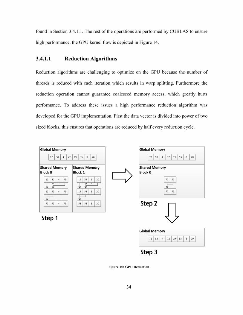
performance. To address these issues a high performance reduction algorithm was
developed for the GPU implementation. First the data vector is divided into power of two
sized blocks, this ensures that operations are reduced by half every reduction cycle.
Figure 15: GPU Reduction
35
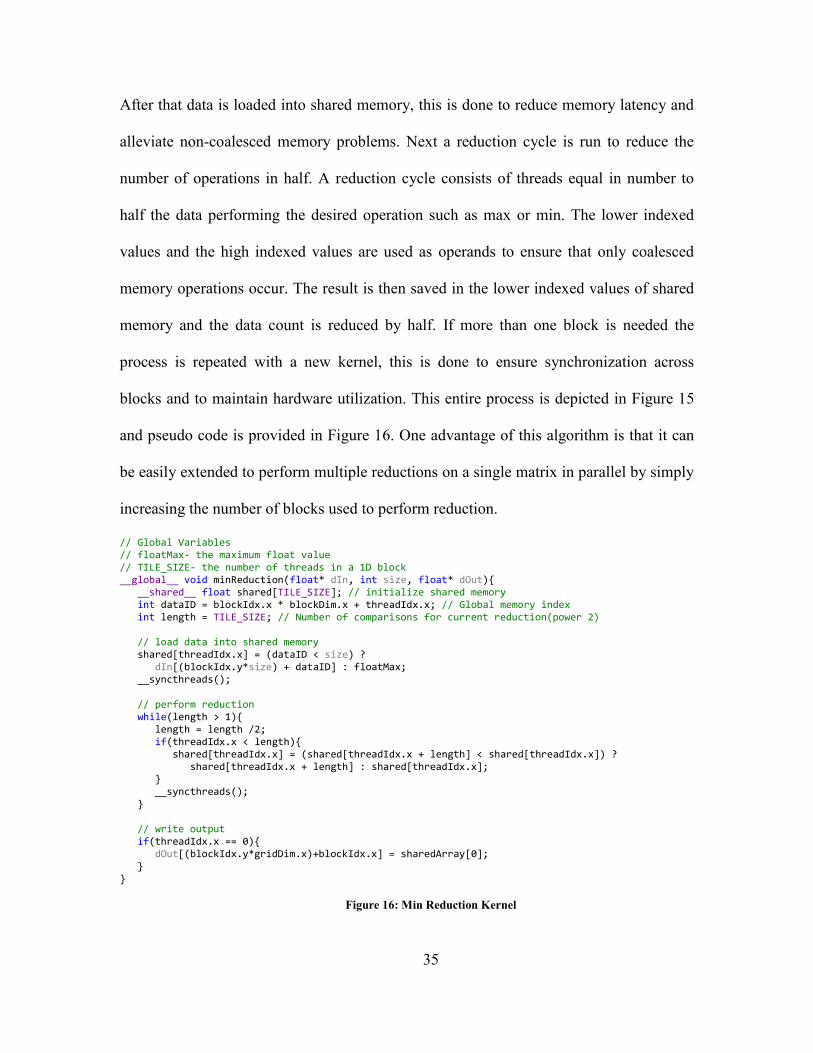
After that data is loaded into shared memory, this is done to reduce memory latency and
alleviate non-coalesced memory problems. Next a reduction cycle is run to reduce the
number of operations in half. A reduction cycle consists of threads equal in number to
half the data performing the desired operation such as max or min. The lower indexed
values and the high indexed values are used as operands to ensure that only coalesced
memory operations occur. The result is then saved in the lower indexed values of shared
memory and the data count is reduced by half. If more than one block is needed the
process is repeated with a new kernel, this is done to ensure synchronization across
blocks and to maintain hardware utilization. This entire process is depicted in Figure 15
and pseudo code is provided in Figure 16. One advantage of this algorithm is that it can
be easily extended to perform multiple reductions on a single matrix in parallel by simply
increasing the number of blocks used to perform reduction.
// Global Variables // floatMax- the maximum float value // TILE_SIZE- the number of threads in a 1D block __global__ void minReduction(float* dIn, int size, float* dOut){ __shared__ float shared[TILE_SIZE]; // initialize shared memory int dataID = blockIdx.x * blockDim.x + threadIdx.x; // Global memory index int length = TILE_SIZE; // Number of comparisons for current reduction(power 2) // load data into shared memory shared[threadIdx.x] = (dataID < size) ? dIn[(blockIdx.y*size) + dataID] : floatMax; __syncthreads(); // perform reduction while(length > 1){ length = length /2; if(threadIdx.x < length){ shared[threadIdx.x] = (shared[threadIdx.x + length] < shared[threadIdx.x]) ? shared[threadIdx.x + length] : shared[threadIdx.x]; } __syncthreads(); } // write output if(threadIdx.x == 0){ dOut[(blockIdx.y*gridDim.x)+blockIdx.x] = sharedArray[0]; } }
Figure 16: Min Reduction Kernel

36
Chapter 4 Experimental Results
4.1. Experimental Setup
For each experiment, the images are converted to greyscale and resized to a final
resolution of 100×90 pixels before performing recognition. Several experiments are run
on occluded versions of various datasets. These datasets are generated by adding
rectangular noise occlusions to 30% of the images in the database. The location of the
rectangular noise is determined randomly, and its size is randomly chosen between 15×15
and 60×60. The noise in the rectangular window consists of normally distributed white
and black pixels.
Eigenface experiments use each test image for single to single classification and
record the average accuracy for a varying number of eigenvectors. For Grassmann
manifold experiments all test images are sorted into their designated class for many to
many classification and the average accuracy for a varying number of Grassmann
eigenvectors is recorded. Each experiments consist of two separate trials of 4-fold cross
validation unless stated otherwise. The accuracies reported are the average accuracies
across both trials.
4.2. Datasets
4.2.1 Yale Face Database
The Yale Face database contains 165 grayscale images of 15 different people
[25]. There are 11 images for each subject and they vary in illumination and facial
expression. Image configuration include centered light, left light, right light, glasses on,
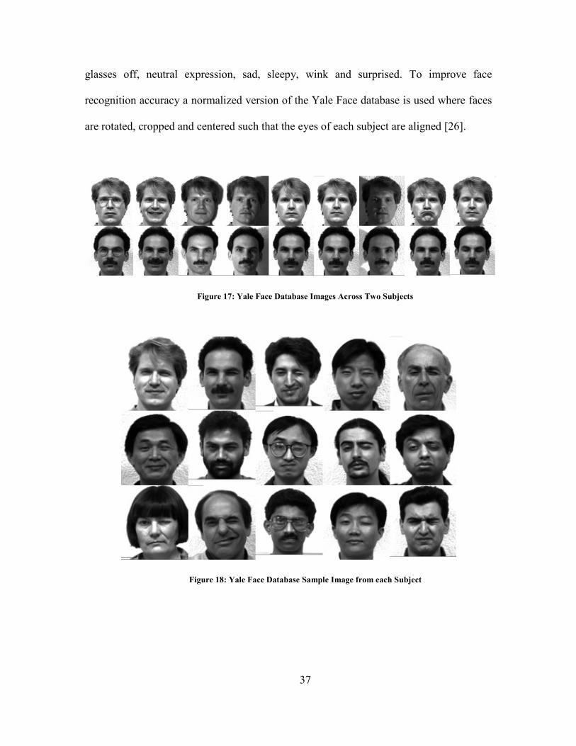
37
glasses off, neutral expression, sad, sleepy, wink and surprised. To improve face
recognition accuracy a normalized version of the Yale Face database is used where faces
are rotated, cropped and centered such that the eyes of each subject are aligned [26].
Figure 17: Yale Face Database Images Across Two Subjects
Figure 18: Yale Face Database Sample Image from each Subject

38
4.2.2 AT&T Database of Faces
This AT&T Database of Faces formerly known as the ORL face database contains
400 images of 40 different people [27]. There are 10 images for each subject and they
vary in pose and facial details such as glasses. Images were taken over time and as a
result minor lighting changes occur across subjects.
Figure 19: AT&T Database Images Across Two Subjects
Figure 20: AT&T Database Sample Image from each Subject

39
4.2.3 Extended Yale Face Database B
The Extended Yale Face Database B contains 2,432 images of 38 different people
[28]. There are 64 images for each subject and they vary in illumination.
Face images vary greatly in illumination across subjects, so much so that at times only a
small portion of the face is visible. To improve face recognition accuracy a close cropped
version of the dataset is used, where each image is cropped to include only the face with
no background or hair.
Figure 21: Extended Yale Face Database B Images Across Two Subjects
Figure 22: Extended Yale Face Database B Sample Image from each Subject

40
4.2.4 AR Face Database
The AR Face Database contains 2,600 color images of 100 different people, 50
men and 50 women [29]. There are 26 images for each subject and they vary in
expression, illumination and natural occlusions. Subjects in this dataset utilize scarfs or
large sun glasses to occlude parts of their face making recognition difficult.
Figure 23: AR Face Database Sample Image from each Subject
41
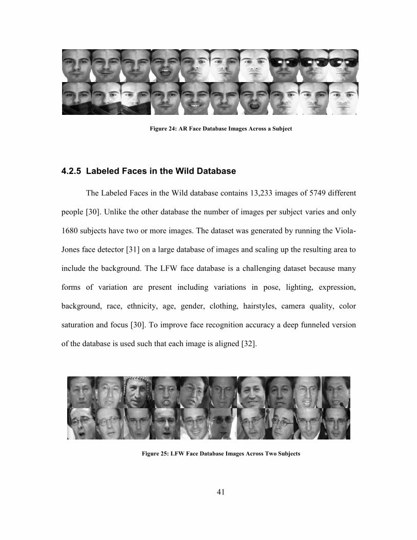
Figure 24: AR Face Database Images Across a Subject
4.2.5 Labeled Faces in the Wild Database
The Labeled Faces in the Wild database contains 13,233 images of 5749 different
people [30]. Unlike the other database the number of images per subject varies and only
1680 subjects have two or more images. The dataset was generated by running the Viola-
Jones face detector [31] on a large database of images and scaling up the resulting area to
include the background. The LFW face database is a challenging dataset because many
forms of variation are present including variations in pose, lighting, expression,
background, race, ethnicity, age, gender, clothing, hairstyles, camera quality, color
saturation and focus [30]. To improve face recognition accuracy a deep funneled version
of the database is used such that each image is aligned [32].
Figure 25: LFW Face Database Images Across Two Subjects
42
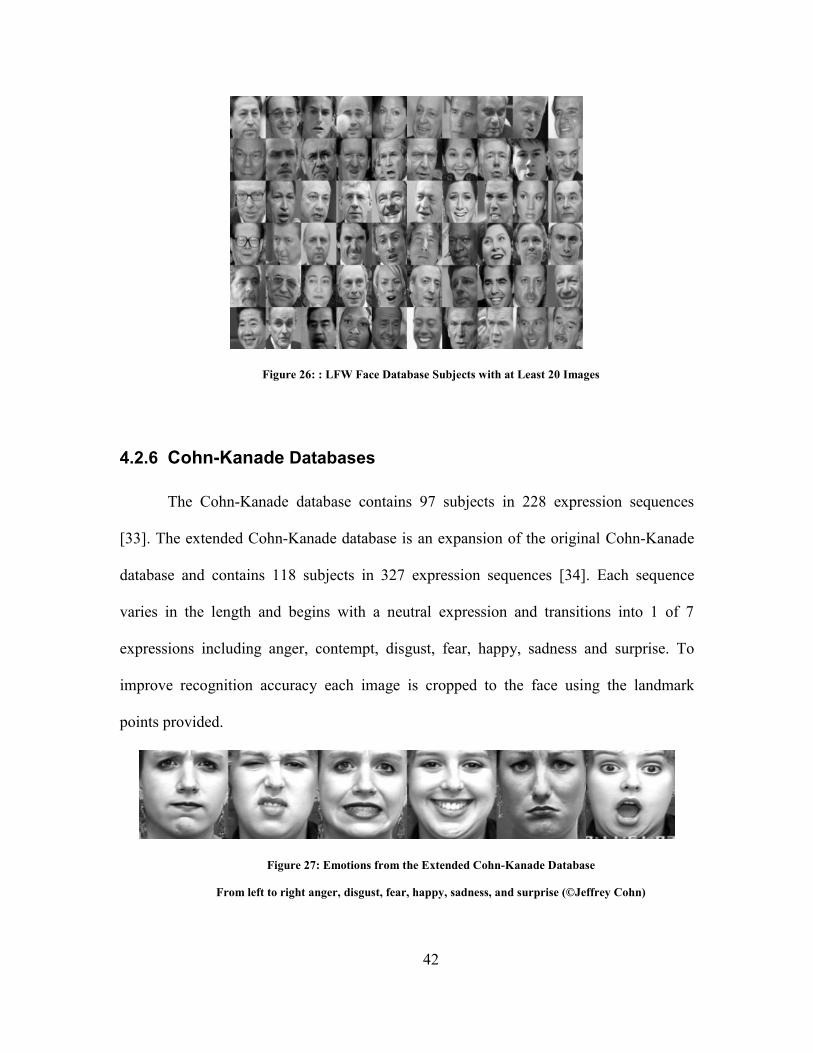
Figure 26: : LFW Face Database Subjects with at Least 20 Images
4.2.6 Cohn-Kanade Databases
The Cohn-Kanade database contains 97 subjects in 228 expression sequences
[33]. The extended Cohn-Kanade database is an expansion of the original Cohn-Kanade
database and contains 118 subjects in 327 expression sequences [34]. Each sequence
varies in the length and begins with a neutral expression and transitions into 1 of 7
expressions including anger, contempt, disgust, fear, happy, sadness and surprise. To
improve recognition accuracy each image is cropped to the face using the landmark
points provided.
Figure 27: Emotions from the Extended Cohn-Kanade Database
From left to right anger, disgust, fear, happy, sadness, and surprise (©Jeffrey Cohn)

43
4.3. Parameter Selection
The maximum number of iterations is used to terminate the eigenvector
optimization process if the algorithm does not converge. The number of iterations
required to optimize the eigenvector is a function of the number of data samples. To
ensure that each binary vector is properly optimized 3N iterations are used. This ensures
that each bit has the chance to be flipped at least three times. In practice most binary
vectors converge in ~2N iterations.
Another important parameter is t which is used to determine the upper and lower
boundaries in the local ternary patterns feature extraction, as shown in (2.32). The
variable t controls how much of the grayscale structure is considered noise. If t is too low,
then LTP captures the noise in smooth areas, however if t is too large LTP does not
capture some of the weaker textures. Some work has been done on picking optimal t
values. In [35] a data adaptive approach was developed that uses Weber's Law and the
central pixel to set t. However, their work was not tested on datasets with variations in
illuminations. In [21] LTP was run extended Yale B and several other datasets with large
variations in illuminations and they found t = 5 is a good threshold for removing
illumination effects. To find the optimal LTP threshold each experiment is repeated for
𝑡 = [1, 20] and the optimal value and its corresponding threshold are reported.
Two parameters that greatly affect the performance of the GPU algorithm are the
main block size and reduction block size. The block size is the number of threads used in
a single CUDA block, to get full GPU utilization the number of threads across all blocks
should be a multiple of 32 so that only full warps are generated. The main block size is
used for all the custom CUDA kernels except for the reduction kernels, which use the

44
reduction block size. The reduction block size has additional constraint; it should be a
power of two so that a full reduction can be performed every reduction cycle. Two GPUs
are used throughout experiments the GeForce GTX 480 and Tesla K20c. The GeForce
GTX 480 can support at maximum 1024 threads per blocks and 1536 threads per
multiprocessor. The optimal main and reduction block size for the GeForce GTX 480 are
768 and 512. The Tesla K20c can support at maximum 1024 threads per blocks and 2048
threads per multiprocessor. The optimal main and reduction block size for the Tesla K20c
are 1024 and 1024.
4.4. Accuracy Tests
In the first two experiments, recognition accuracy was collected from the Yale,
AT&T and extended Yale databases. All data was normalized and centered such that the
mean was zero and the standard deviation was one. Results were collected using a variant
of four fold cross validation that ensured the number of images of a person was the same
for each fold. In the first experiment the 𝐿1-eigenfaces and 𝐿1-Grassmann face
recognition techniques are compared against the 𝐿2 versions on the original databases.
This test ensures that the suboptimal methods utilized to accelerate 𝐿1-PCA do not
negatively affect the recognition accuracy. Twenty five iterations of 4 fold cross
validation was used to establish a baseline for the eigenface comparison.

45
Figure 28: Eigenface Comparison Test Yale Database
Figure 29: Eigenface Comparison Test AT&T Database

46
Figure 30: Grassmann Comparison Test Yale Database
Figure 31: Grassmann Comparison Test AT&T Database

47
Figure 32: Grassmann Comparison Test Extended Yale B Database
All of the 𝐿1-PCA based techniques performed as good as or better than the 𝐿2-
PCA based techniques indicating that the suboptimal methods utilized by 𝐿1-PCA did not
negatively affect recognition performance. Furthermore 𝐿1-Grassmann outperformed 𝐿2-
Grassmann by ~10% on the Yale database Figure 30. The Yale database has the fewer
images per subject than any other databases tested, as a result when the Grassmann
manifold is being formed noise has a greater influence. 𝐿1-PCA was able to mitigate the
effect of the noise and as a result improve recognition for 𝐿1-Grassmann.
In the second experiment rectangular occlusions are added to 30% of all images in
each database and the procedure from the first experiment is repeated on the occluded
datasets. This experiment highlights the effectiveness of 𝐿1-PCA at reducing the impact
of noise in face recognition techniques. Once again 𝐿1-Eigenfaces was run for 25
iterations of 4 fold cross validation.

48
Figure 33: Eigenfaces Comparison Test Occluded Yale Database
Figure 34: Eigenfaces Comparison Test Occluded AT&T Database
49
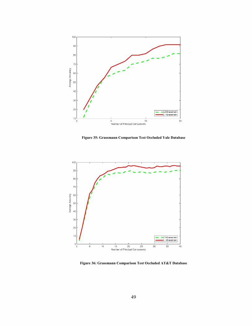
Figure 35: Grassmann Comparison Test Occluded Yale Database
Figure 36: Grassmann Comparison Test Occluded AT&T Database
50
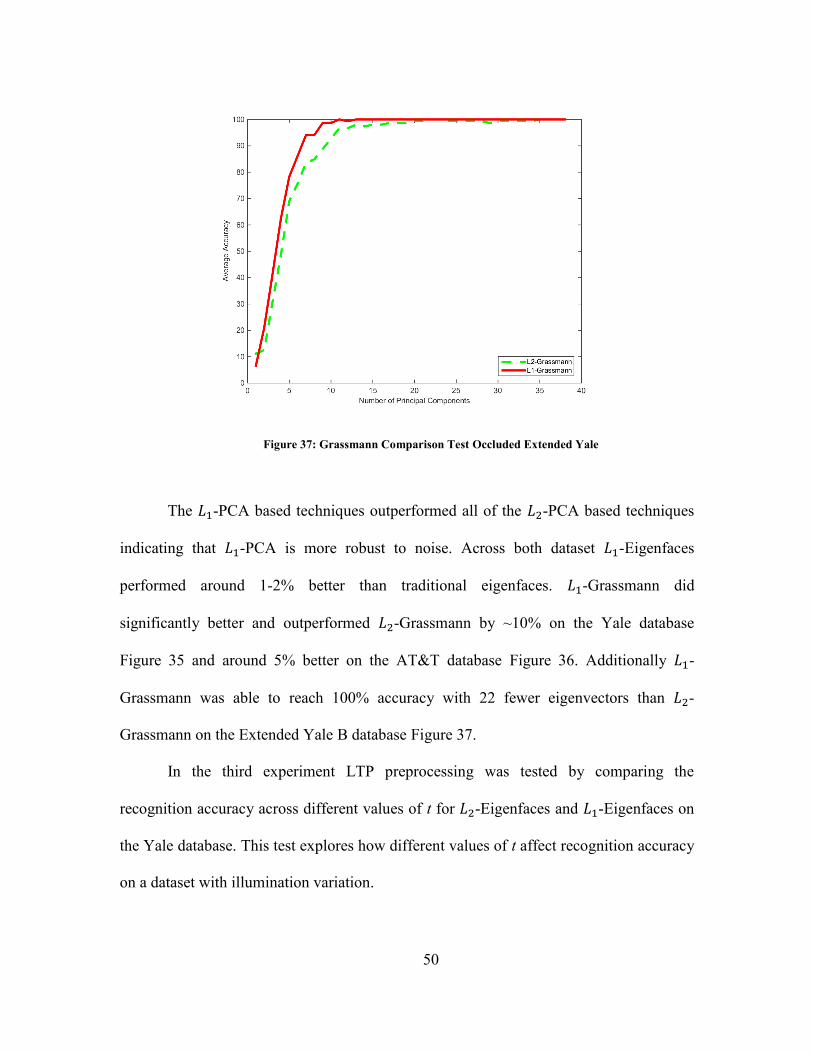
Figure 37: Grassmann Comparison Test Occluded Extended Yale
The 𝐿1-PCA based techniques outperformed all of the 𝐿2-PCA based techniques
indicating that 𝐿1-PCA is more robust to noise. Across both dataset 𝐿1-Eigenfaces
performed around 1-2% better than traditional eigenfaces. 𝐿1-Grassmann did
significantly better and outperformed 𝐿2-Grassmann by ~10% on the Yale database
Figure 35 and around 5% better on the AT&T database Figure 36. Additionally 𝐿1-
Grassmann was able to reach 100% accuracy with 22 fewer eigenvectors than 𝐿2-
Grassmann on the Extended Yale B database Figure 37.
In the third experiment LTP preprocessing was tested by comparing the
recognition accuracy across different values of t for 𝐿2-Eigenfaces and 𝐿1-Eigenfaces on
the Yale database. This test explores how different values of t affect recognition accuracy
on a dataset with illumination variation.

51
Figure 38: LTP L2-Eigenface t Test for Yale Database
Figure 39: LTP L1-Eigenface t Test for Yale Database
52
This experiment shows that the actual t value chosen for LTP does not have a
significant impact on recognition performance. The results for 𝐿2-Eigenfaces in Figure 38
show that accuracy varies on average by ~3% between t values. The results for 𝐿1-
Eigenfaces in Figure 39 show that accuracy varies on average by ~3% between t values.
In general, a t value of 2 is recommended for face recognition because it produces good
recognition results across the Yale, AT&T and extended Yale database for LTP 𝐿2-
Eigenfaces.
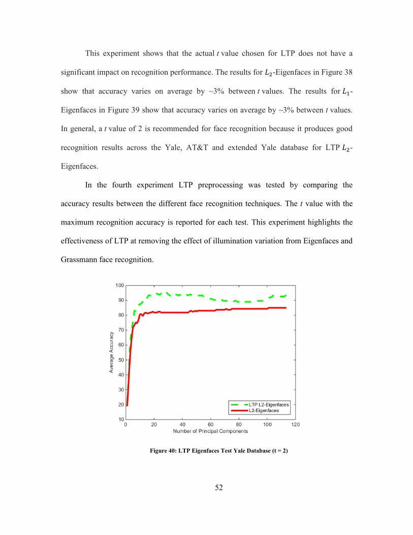
In the fourth experiment LTP preprocessing was tested by comparing the
accuracy results between the different face recognition techniques. The t value with the
maximum recognition accuracy is reported for each test. This experiment highlights the
effectiveness of LTP at removing the effect of illumination variation from Eigenfaces and
Grassmann face recognition.
Figure 40: LTP Eigenfaces Test Yale Database (t = 2)

53
Figure 41: LTP Eigenfaces Test AT&T Database (t = 6)
Figure 42: LTP Eigenfaces Test Extended Yale B Database (t = 1)

54
Figure 43: LTP Grassmann Test Yale Database (t = 5)
Figure 44: LTP Grassmann Test AT&T Database (t = 6)

55
Figure 45: LTP Grassmann Test Extended Yale B Database (t = 5)
LTP with 𝐿2-Eigenfaces outperformed traditional 𝐿2-Eigenfaces (without LTP)
by about ~15% on both Yale Figure 40 and the Extended Yale database Figure 42.
However, they performed significantly worse on the AT&T database Figure 41. LTP
characterizes the underlying greyscale structure which allows it to perform well on
datasets with great variation in illumination. However, when LTP is used to preprocess
images it throws away the actual intensity values of the pixels which can be useful for
recognition if the dataset of the underlying grey level structure is apparent. Since the
AT&T database does not contain a significant amount of variation in illumination the
traditional 𝐿2-Eigenfaces works better because it has more information to work with.
Another major feature of the results is that the recognition accuracy degrades after
a certain number of principal components. LTP preprocessing has a larger dimensionality
because its feature vector is a concatenation of the upper and lower images and as a result

56
we approach a special case for principal component analysis where we have data that has
large dimensionality and few samples. In [36] this special usage case is explored and they
find that if the first few principal components capture most of the variance, then the other
principal components will not converge to the appropriate subspace. As a result it is
advisable to choose only a modest number of principal components to maximize
recognition accuracy when using LTP preprocessing.
The LTP 𝐿2-Grassmann also outperformed traditional 𝐿2-Grassmann, on the Yale
database LTP was ~18% better Figure 43 and on the Extended Yale B database Figure 45
it converged to 100% accuracy with 5 fewer principal components. Once again LTP was
outperformed on the AT&T database Figure 44, due to the missing information.
In the fifth experiment LTP 𝐿1-Grassmann and LTP 𝐿2-Grassmann is run on the
Yale, AT&T, Extended Yale B, AR, LFW, Cohn-Kanade and Extended Cohn-Kanade
databases. For the expression recognition experiments only happy, sadness, surprise and
anger are used, while disgust and fear were ignored. To ensure accurate results the
average accuracy from ten iterations of ten-fold cross validation are reported for
expression recognition. This test is meant to evaluate the optimal performance of these
recognition methods on challenging datasets.
Across all of the databases, LTP 𝐿1-Grassmann performed as good as or better
than LTP 𝐿2-Grassmann. Both 𝐿1 and 𝐿2 LTP Grassmann reached 100% recognition
accuracy on the Yale Figure 46, extended Yale B Figure 48 and the AR databases Figure
49. LTP 𝐿1-Grassmann outperformed LTP 𝐿2-Grassmann by 0.63% on the AT&T
database Figure 47, 3.23% on the LFW database Figure 50, 2.25% on the Cohn-Kanade
database Figure 51 and 1.75% on the extended Cohn-Kanade database Figure 52.

57
Figure 46: LTP Grassmann Yale Database (t = 5)
Figure 47: LTP Grassmann AT&T Database (t = 6)

58
Figure 48: LTP Grassmann Extended Yale B Database (t = 5)
Figure 49: LTP Grassmann AR Database (t = 5)

59
Figure 50: LTP Grassmann LFW Database (t = 5)
Figure 51: LTP Grassmann Cohn-Kanade Database (t = 14)

60
Figure 52: LTP Grassmann Extended Cohn-Kanade Database (t = 16)
This indicates that databases with a small amount of noise or a large number of
data samples may get the similar results as LTP 𝐿1-Grassmann. Conversely, datasets with
large amounts of noise like LFW or a small number of data samples like the Cohn-
Kanade database get better results with LTP 𝐿1-Grassmann. Another interesting
observation from these results is that the optimal LTP value is much larger for expression
recognition. The larger LTP most likely removes some of the finer features of the faces
that are not need for expression recognition but are need for face recognition.
In the final experiment LTP 𝐿1-Grassmann was run on a varying number of
images per subjects from LFW database. This experiment is repeated ten times and the
average accuracy is reported. This test is meant to evaluate the effect of the number of
data samples on accuracy.
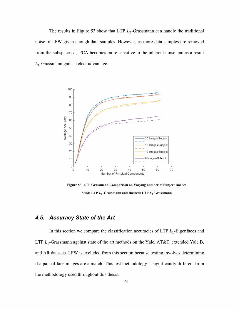
61
The results in Figure 53 show that LTP 𝐿2-Grassmann can handle the traditional
noise of LFW given enough data samples. However, as more data samples are removed
from the subspaces 𝐿2-PCA becomes more sensitive to the inherent noise and as a result
𝐿1-Grassmann gains a clear advantage.
Figure 53: LTP Grassmann Comparison on Varying number of Subject Images
Solid: LTP 𝑳𝟏-Grassmann and Dashed: LTP 𝑳𝟐-Grassmann
4.5. Accuracy State of the Art
In this section we compare the classification accuracies of LTP 𝐿1-Eigenfaces and
LTP 𝐿1-Grassmann against state of the art methods on the Yale, AT&T, extended Yale B,
and AR datasets. LFW is excluded from this section because testing involves determining
if a pair of face images are a match. This test methodology is significantly different from
the methodology used throughout this thesis.
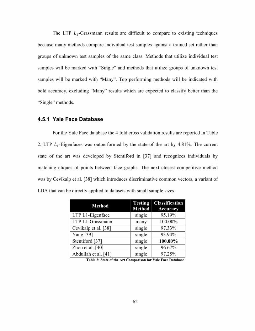
62
The LTP 𝐿1-Grassmann results are difficult to compare to existing techniques
because many methods compare individual test samples against a trained set rather than
groups of unknown test samples of the same class. Methods that utilize individual test
samples will be marked with “Single” and methods that utilize groups of unknown test
samples will be marked with “Many”. Top performing methods will be indicated with
bold accuracy, excluding “Many” results which are expected to classify better than the
“Single” methods.
4.5.1 Yale Face Database
For the Yale Face database the 4 fold cross validation results are reported in Table
2. LTP 𝐿1-Eigenfaces was outperformed by the state of the art by 4.81%. The current
state of the art was developed by Stentiford in [37] and recognizes individuals by
matching cliques of points between face graphs. The next closest competitive method
was by Cevikalp et al. [38] which introduces discriminative common vectors, a variant of
LDA that can be directly applied to datasets with small sample sizes.
Method Testing
Method
Classification
Accuracy
LTP L1-Eigenface single 95.19%
LTP L1-Grassmann many 100.00%
Cevikalp et al. [38] single 97.33%
Yang [39] single 93.94%
Stentiford [37] single 100.00%
Zhou et al. [40] single 96.67%
Abdullah et al. [41] single 97.25% Table 2: State of the Art Comparison for Yale Face Database

63
4.5.2 AT&T Database of Faces
For the AT&T Database of Faces the 4 fold cross validation results are reported in
Table 3. LTP 𝐿1-Eigenfaces was outperformed by the state of the art by 10.97% and LTP
𝐿1-Grassmann was outperformed by 3.75%. The leading method is presented by Othman
et al. in [42] in which they use 2D-Hidden Markov Models perform recognition using the
image pixels as features. The next closest competitive method was by Lenc in [43] in
which they identify key-points from Gabor wavelet using k-means with LBP.
Method Testing
Method
Classification
Accuracy
LTP L1-Eigenface single 88.83%
LTP L1-Grassmann many 96.25%
Azary [44] single 99.00%
Azary [44] many 100.00%
Faraji & Qi [45] single 98.87%
Othman et al. [42] single 100%
Lenc & Král [43] single 99.80% Table 3: State of the Art Comparison for AT&T Database of Faces
4.5.3 Extended Yale Face Database B
The leading method is presented by Kumar et al. in [46] in which they learn a
series of convolution filters to extract features and then apply boosting to perform
recognition. The next closest competitive method was by Azary in [44] in which he
utilizes Grassmannian Sparse Representations for “Single” and Grassmannian Spectral
Regression for “Many” tests.

64
Method Testing
Method
Classification
Accuracy
LTP L1-Grassmann many 100.00%
Azary [44] single 98.89%
Azary [44] many 100.00%
Fernandes & Bala [47] single 97.50%
Cai et al. [48] single 95.17%
Kumar et al. [46] single 99.6% Table 4: State of the Art Comparison for Extended Yale B Face Database
4.5.4 AR Face Database
For the AR Database of Faces the 4 fold cross validation results are reported in
Table 5. LTP 𝐿1-Grassmann outperformed state of the art by 21.69%, however state of
the art utilized the “Single” testing methodology. The leading method is presented by
Andrés et al. in [49] in which they detect the occlusions and utilize the non-occluded
regions to perform recognition. The next closest competitive method was by Liu et al.
[50] which reports 95.30% accuracy on the AR Database of Faces using 𝐿2-norm
regularization to learn a dictionary more suitable for face recognition from face
reconstruction error.
Method Testing
Method
Classification
Accuracy
LTP L1-Grassmann many 100.00%
Xuefeng et al. [51] single 95.20%
Lin et al. [52] single 91.50%
Martinez [53] single 85.00%
Andrés et al. [49] single 98.31%
Liu et al. [50] single 95.30% Table 5: State of the Art Comparison for AR Face Database
65
4.6. Speed tests
For the GPU benchmark the number of data samples was varied to see how each
implementation scaled to larger datasets. All the images were taken from the labeled
faces in the wild dataset and were cropped such that only the face was visible [54].
Images were added incrementally to form test sets with varying number of samples and
each test set is scaled and centered before running 𝐿1-PCA. The timing is collected for
the first fifty eigenvectors of each test set. For test sets with fewer eigenvectors the timing
is repeated ten times to get the average performance time. All performance experiments
were performed on a 64-bit Windows 7 machine with an Intel Core i5-2400 3.10-GHz
CPU and 8 GB of RAM. The NVIDIA GTX 480 and NVIDIA Tesla K20c were used for
GPU experiments, both used the CUDA 5.0 driver.
As expected the time complexity of the 𝐿1-PCA algorithm is quadratic in relation
to the number of data samples as shown in Figures 54, 55 and 56. The CPU runtime is
several orders of magnitude larger than the GTX and Tesla runtime.
The GTX speedup varies from 2x to 9.4x and the Tesla speedup is from 7.4x to
21.5x faster as shown in Figures 57 and 58. In both speedup graphs there are data points
where the performance suddenly drops. These performance drops indicate that the GPU
utilization has decreased and are the result of edge cases between block sizes. The drop in
performance occurs at 960 data samples on the GTX where the block size is 768. With
that block size there will be 1 block with full utilization and a second block with 75% of
the threads being stalls. Similarly a drop in performance occurs at 1280 data samples on
the Tesla card where the block size is 1024.

66
Figure 54: CPU Timing
Figure 55: GTX Timing

67
Figure 56: Tesla Timing
Figure 57: GTX Speedup
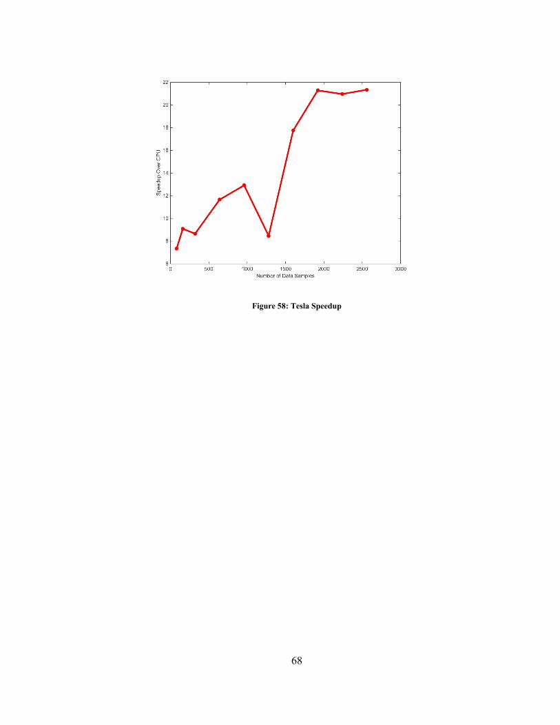
68
Figure 58: Tesla Speedup

69
Chapter 5 Conclusion and Future Work
The aim of this thesis was to develop recognition algorithms that leverages 𝐿1-
PCA to improve accuracy in unconstrained environments. The following contributions to
the field of recognition were presented in this work:
An extension of an 𝐿1 Principal Component algorithm to multiple components
A high performance implementation of 𝐿1-PCA on GPU using CUDA
An 𝐿1-PCA mapping for Grassmann manifolds
An extension of 𝐿1-Grassmann using LTP
Despite the suboptimal methods that were employed for 𝐿1-PCA, recognition accuracy
was not negatively affected for clean images. Furthermore, 𝐿1-eigenfaces outperformed
𝐿2-eigenfaces when occlusions were added to the data, which indicates that 𝐿1-PCA is
more robust to outliers. The results also show that the proposed 𝐿1-Grassmann approach
outperformed the traditional 𝐿2-Grassmann method for face recognition of clean and
occluded faces. This indicates that mapping to the Grassmann manifold is very sensitive
to noise and benefits from the more robust mapping systems. Additionally, 𝐿1-Grassmann
has been generic enough to be applied to other recognition tasks such as facial expression
recognition. This work has also shown that the proposed 𝐿1-PCA algorithm can greatly
benefit from a GPU implementation. The high performance implementation was several
times faster than the CPU based 𝐿1-PCA techniques allowing it to run on larger datasets
in a reasonable amount of time. Lastly the LTP preprocessing removed the effects of
varying illumination and improved the accuracy of both techniques on databases with
large variations in illumination.
70
One problem that plagues the suboptimal 𝐿1-PCA, is that the later eigenvectors
tend to capture the noise in the images. This is caused by the suboptimal greedy search
removing good features until there is nothing, but noise left. This factor leads to
complications when many eigenvectors are needed for applications such as 𝐿1-
Eigenfaces. If too many eigenvectors are used, the noise in the image will begin to affect
the results and performance will become similar to 𝐿2-eigenfaces. Conversely, if too few
eigenvectors are used, the features will not be specific enough to distinguish between
subjects. Thus, the best performance is achieved with a modest number of eigenvectors.
The potential solution is to develop an algorithm that solves for all 𝐿1-eigenvectors
simultaneously. However, this fundamentally changes the contribution calculation such
that the bit-flip algorithm would no longer work. In the past, authors have used an
exhaustive search over 2𝑁𝑀 binary matrices of size 𝑁 × 𝑀, where N is the number of
data samples and M is the number of eigenvectors to solve for all 𝐿1-eigenvectors
simultaneously [9].
Additionally the Grassmann algorithm has experienced difficulty recognizing
subjects when there are few training or test images per subject. Several images of the
subject are needed to properly map images to points on the Grassmann. Too few images
causes the points on the Grassmann to be too general which results in poor performance.
One potential method for mitigating such a problem is to artificially expand the number
of images using techniques like affine transformation. This would allow the Grassmann
manifold to capture the in-class variability for sparse classes and improve performance.
In conclusion, this work has demonstrated that 𝐿1-PCA improves the robustness
of recognition techniques such as Eigenfaces and Grassmann learning. Furthermore

71
experimental results have shown that 𝐿1-PCA has the potential to be greatly accelerated
using the GPGPU.
72
Bibliography
[1] R. Jafri and H. R. Arabnia, "A Survey of Face Recognition Techniques," JIPS, vol.
5, no. 2, pp. 41-68, 2009.
[2] N. Funatsu and Y. Kuroki, "Fast parallel processing using GPU in computing L1-
PCA bases," TENCON, pp. 2087-2090, 2010.
[3] J. Hamm and D. D. Lee, "Grassmann discriminant analysis: a unifying view on
subspace-based learning," Proceedings of the 25th international conference on
Machine learning, pp. 376-383, 2008.
[4] P. Turaga, A. Veeraraghavan and R. Chellappa, "Statistical analysis on Stiefel and
Grassmann manifolds with applications in computer vision," Computer Vision and
Pattern Recognition, pp. 1-8, 2008.
[5] K. Pearson, "On Lines and Planes of Closest Fit to Systems," The London,
Edinburgh, and Dublin Philosophical Magazine and Journal of Science, vol. 2, no.
11, pp. 559-572, 1901.
[6] J. Shlens, "A Tutorial on Principal Component Analysis," CoRR, vol. abs/1404.1100,
2014.
[7] P. P. Markopoulos, G. Karystinos and D. Pados, "Some options for L1-subspace
signal processing," Proc. Tenth Int. Symposium on Wireless Communication
Systems, 2013.
[8] N. Kwak, "Principal Component Analysis Based on L1-norm Maximization," IEEE
Transactions on Pattern Analysis and Machine Intelligence, PAMI, 2008.
73
[9] P. P. Markopoulos, G. N. Karystinos and D. A. Pados, "Optimal Algorithms for L1-
subspace Signal Processing," IEEE Transactions on Signal Processing, 2013.
[10] Q. Ke and T. Kanade, "Robust L1 Factorization in the Presence of Outliers and
Missing Data by Alternative Convex Programming," CVPR, pp. 739-746, 2005.
[11] F. Nie, H. Huang, C. Ding, D. Luo and H. Wang, "Robust principal component
analysis with non-greedy l1-norm maximization," IJCAI Proc. Int. Joint Conference
on Artificial Intelligence, vol. 22, no. 1, 2011.
[12] S. Kundu, P. P. Markopoulos and D. A. Pados, "Fast computation of the L1-principal
component of real-valued data," Proceedings of 39th IEEE International Conference
on Acoustics Speech and Signal Processing, ICASSP, 2014.
[13] M. Kirby and L. Sirovich, "Application of the Karhunen-Loeve Procedure for the
Characterization of Human Faces," IEEE Transactions on Pattern Analysis and
Machine Intelligence, vol. 12, no. 1, pp. 103-108, 1990.
[14] M. Turk and A. Pentland, "Face recognition using eigenfaces," IEEE Conference on
Computer Vision and Pattern Recognition, CVPR, 1991.
[15] A. Pentland, B. Moghaddam and T. Starner, "View-based and modular eigenspaces
for face recognition," Computer Vision and Pattern Recognition, vol. CVPR'94,
1994.
[16] R. Gottumukkal and V. K. Asari, "An improved face recognition technique based on
modular PCA approach," Pattern Recognition Letters, vol. 25, no. 4, pp. 429-436,
2004.
[17] J. Yang, D. Zhang, A. Frangi and J.-y. Yang, "Two-dimensional PCA: a new

74
approach to appearance-based face representation and recognition," Pattern Analysis
and Machine Intelligence, vol. 26, no. 1, pp. 131-137, 2004.
[18] R. Shigenaka, B. Raytchev, T. Tamaki and K. Kaneda, "Face sequence recognition
using Grassmann distances and Grassmann kernels," Neural Networks (IJCNN), pp.
1-7, 2012.
[19] S. Azary and A. Savakis, "Grassmannian Sparse Representations and Motion Depth
Surfaces for 3D Action Recognition," Computer Vision and Pattern Recognition
Workshops (CVPRW), 2013.
[20] T. Ojala, M. Pietikainen and T. Maenpaa, "Multiresolution Gray Scale and Rotation
Invariant Texture Classification," Pattern Analysis Machine Intelligence, vol. 24, no.
7, pp. 971-987, 2002.
[21] X. Tan and B. Triggs, "Enhanced Local texture Feature Sets for Face Recognition
Under Difficult Lighting Conditions," Transactions on Image Processing, vol. 19,
no. 6, pp. 1635-1650, 2010.
[22] NVIDIA, "CUDA C Programing Guide v6.0," 13 February 2014. [Online].
Available: http://docs.nvidia.com/cuda/cuda-c-programming-
guide/index.html#axzz36kgvGYg4.
[23] F. Zhong, "L1-norm-based (2D)^2PCA," Conference on Computer Science and
Electrical Engineering, pp. 1293-1296, 2013.
[24] T. Shakunaga and K. Shigenari, "Decomposed eigenface for face recognition under
various lighting conditions," Proceedings of the 2001 IEEE Conference on Computer
Vision and Pattern Recognition, CVPR, 2001.

75
[25] P. Belhumeur, J. Hespanha and D. Kriegman, "Eigenfaces vs. fisherfaces:
Recognition using class specific linear projection," IEEE Transactions on Pattern
Analysis and Machine Intelligence, PAMI, pp. 711-720, 1997.
[26] D. Roy, "The Normalized Yale Face Database," MIT, 01 September 2000. [Online].
Available: http://vismod.media.mit.edu/vismod/classes/mas622-00/datasets/.
[27] F. S. Samaria and A. C. Harter, "Parameterisation of a stochastic model for human
face identification," Applications of Computer Vision, pp. 138-142, 1994.
[28] A. S. Georghiades, P. N. Belhumeur and D. J. Kriegman, "From Few to Many:
Illumination Cone Models for Face Recognition under Variable Lighting and Pose,"
IEEE Transactions on Pattern Analysis and Machine Intelligence, vol. 23, pp. 643-
660, 2001.
[29] A. M. Martinez and R. Benavente, "The AR Face Database," 1998.
[30] G. B. Huang, M. Ramesh, T. Berg and E. Learned-Miller, "Labeled Faces in the
Wild: A Database for Studying," University of Massachusetts, Amherst, 2007.
[31] P. Viola and M. J. Jones, "Robust real-time face detection," International journal of
computer vision, vol. 57, no. 2, pp. 137-154, 2004.
[32] G. Huang, M. Mattar, H. Lee and E. G. Learned-Miller, "Learning to align from
scratch," Advances in Neural Information Processing Systems, pp. 764-772, 2012.
[33] T. Kanade, J. F. Cohn and Y. Tian, "Comprehensive database for facial expression
analysis," Proceedings of the Fourth IEEE International Conference on Automatic
Face and Gesture Recognition , pp. 46-53, 2000.
[34] P. Lucey, J. F. Cohn, T. Kanade, J. Saragih, Z. Ambadar and I. Matthews, "The

76
Extended Cohn-Kanade Dataset (CK+): A complete expression dataset for action
unit and emotion-specified expression," Proceedings of the Third International
Workshop on CVPR for Human Communicative Behavior Analysis , pp. 94-101,
2010.
[35] Z. Wang, R. Huang, W. Yang and C. Sun, "An enhanced Local Ternary Patterns
method for face recognition," Control Conference, vol. 33, pp. 4636-4640, 2014.
[36] S. Jung and J. S. Marron, "PCA consistency in high dimension, low sample size
context," The Annals of Statistics, vol. 37, no. 6B, pp. 4104-4130, 2009.
[37] F. Stentiford, "Face recognition by detection of matching cliques of points,"
IS&T/SPIE Electronic Imaging, 2014.
[38] H. Cevikalp, M. Neamtu, M. Wilkes and A. Barkana, "Discriminative common
vectors for face recognition," Pattern Analysis and Machine Intelligence, vol. 27, no.
1, pp. 4-13, 2005.
[39] M.-H. Yang, "Kernel eigenfaces vs. kernel fisherfaces: Face recognition using kernel
methods," Automatic Face and Gesture Recognition, vol. 10, pp. 0215-0215, 2013.
[40] L. Zhou, Y. Xu, Z.-M. Lu and T. Nie, "Face recognition based on multi-wavelet and
sparse representation," J. Inf. Hiding Multimed. Signal Process, vol. 5, no. 3, pp.
399-407, 2014.
[41] M. F. A. Abdullah, M. S. Sayeed, K. S. Muthu, H. K. Bashier, A. Azman and S. Z.
Ibrahim, "Face recognition with symmetric local graph structure (slgs)," Expert
Systems with Applications, vol. 41, no. 14, pp. 6131-6137, 2014.
[42] H. Othman and T. Aboulnasr, "A separable low complexity 2D HMM with

77
application to face recognition," Pattern Analysis and Machine Intelligence, vol. 25,
no. 10, pp. 1229-1238, 2003.
[43] L. Lenc and P. Král, "Automatically Detected Feature Positions for LBP Based Face
Recognition," Artificial Intelligence Applications and Innovations, pp. 246-255,
2014.
[44] S. Azary, "Grassmann Learning for Recognition and Classification," Rochester
Institute of Technology, Rochester, 2014.
[45] M. R. Faraji and X. Qi, "An effective neutrosophic set-based preprocessing method
for face recognition," Multimedia and Expo Workshops, 2013.
[46] R. Kumar, A. Banerjee, B. Vemuri and H. Pfister, "Trainable convolution filters and
their application to face recognition," Pattern Analysis and Machine Intelligence,
vol. 7, no. 34, pp. 1423-1436, 2012.
[47] S. Fernandes and J. Bala, "Performance Analysis of PCA-based and LDA-based
Algorithms for Face Recognition," Signal Processing Systems, vol. 1, no. 1, pp. 1-6,
2013.
[48] D. Cai, X. He, J. Han and H. Zhang, "Orthogonal laplacianfaces for face
recognition," Image Processing, vol. 15, no. 11, pp. 3608-3614, 2006.
[49] M. A. Andrés, S. Padovani, M. Tepper and J. Jacobo-Berlles, "Face recognition on
partially occluded images using compressed sensing," Pattern Recognition Letters,
vol. 36, pp. 235-242, 2014.
[50] H.-D. Liu, M. Yang, Y. Gao, Y. Yin and L. Chen, "Bilinear discriminative dictionary
learning for face recognition," Pattern Recognition, vol. 47, no. 5, pp. 1835-1845,
78
2014.
[51] C. Xuefeng, L. Fei and C. Huang, "Face recognition by Zero-Ratio based LGBP
features," Intelligent Control and Automation (WCICA), vol. 11, pp. 5605-5608,
2014.
[52] J. Lin, J. Ming and D. Crookes, "Robust face recognition with partially occluded
images based on a single or a small number of training samples," Speech and Signal
Processing, pp. 881-884, 2009.
[53] A. M. Martínez, "Recognizing imprecisely localized, partially occluded, and
expression variant faces from a single sample per class," Pattern Analysis and
Machine Intelligence, vol. 24, no. 6, pp. 748-763, 2002.
[54] B. Gary, H. Ramesh, M. Ramesh, T. Berg and E. Learned-Miller, "Labeled Faces in
the Wild: A Database for Studying," University of Massachusetts, Amherst, 2007.
[55] M. Johnson and A. Savakis, "Fast L1-eigenfaces for robust face recognition,"
Western New York Image and Signal Processing Workshop (WNYISPW), 2014.