citation: ozoemena, matthew (2016) sustainability ...nrl.northumbria.ac.uk/27221/1/final phd thesis...

Citation: Ozoemena, Matthew (2016) Sustainability Assessment of Wind Turbine Design Variations: An Analysis of the Current Situation and Potential Technology Improvement Opportunities. Doctoral thesis, Northumbria University.

This version was downloaded from Northumbria Research Link: http://nrl.northumbria.ac.uk/27221/

Northumbria University has developed Northumbria Research Link (NRL) to enable users to access the University’s research output. Copyright © and moral rights for items on NRL are retained by the individual author(s) and/or other copyright owners. Single copies of full items can be reproduced, displayed or performed, and given to third parties in any format or medium for personal research or study, educational, or not-for-profit purposes without prior permission or charge, provided the authors, title and full bibliographic details are given, as well as a hyperlink and/or URL to the original metadata page. The content must not be changed in any way. Full items must not be sold commercially in any format or medium without formal permission of the copyright holder. The full policy is available online: http://nrl.northumbria.ac.uk/policies.html

http://nrl.northumbria.ac.uk/policies.html

Sustainability Assessment of Wind

Turbine Design Variations: An Analysis

of the Current Situation and Potential

Technology Improvement Opportunities

M C OZOEMENA

PhD

2015

Sustainability Assessment of Wind Turbine

Design Variations: An Analysis of the

Current Situation and Potential Technology

Improvement Opportunities

Matthew Chibuikem Ozoemena

A thesis submitted in partial fulfilment of the

requirements of the University of Northumbria

at Newcastle for the degree of Doctor of

Philosophy

Research undertaken in the Faculty of

Engineering and Environment

December 2015

Abstract

Over the last couple of decades, there has been increased interest in environmentally

friendly technologies. One of the renewable energy sources that has experienced huge

growth over the years is wind power with the introduction of new wind farms all over

the world, and advances in wind power technology that have made this source more

efficient. This recognition, together with an increased drive towards ensuring the

sustainability of wind energy systems, has led many to forecast the drivers for future

performance.

This study aims to identify the most sustainable wind turbine design option for future

grid electricity within the context of sustainable development. As such, a methodology

for sustainability assessment of different wind turbine design options has been

developed taking into account environmental, data uncertainty propagation and

economic aspects. The environmental impacts have been estimated using life cycle

assessment, data uncertainty has been quantified using a hybrid DQI-statistical method,

and the economic assessment considered payback times. The methodology has been

applied to a 1.5 MW wind turbine for an assessment of the current situation and

potential technology improvement opportunities.

The results of this research show that overall, the design option with the single-

stage/permanent magnet generator is the most sustainable. More specifically, the

baseline turbine performs best in terms of embodied carbon and embodied energy

savings. On the other hand, the design option with the single-stage/permanent magnet

generator performs best in terms of wind farm life cycle environmental impacts and

payback time compared to the baseline turbine. With respect to the design options with

increased tower height, it is estimated that both designs are the least preferred options

given their payback times. Therefore, the choice of the most sustainable design option

depends crucially on the importance placed on different sustainability indicators which

should be acknowledged in decision making and policy.

i

List of Contents Abstract .............................................................................................................................. i

List of Contents ................................................................................................................. ii

List of Figures .................................................................................................................. ix

List of Abbreviations...................................................................................................... xiv

Acknowledgements ....................................................................................................... xvii

Declaration ................................................................................................................... xviii

Chapter 1 Introduction ................................................................................................. 1

1.1 Sustainable Development ................................................................................... 1

1.2 Energy Supply and the Environment .................................................................. 2

1.3 Justification for Wind Power in the Overall Energy Context ............................ 2

1.3.1 Wind - What Is It? ....................................................................................... 3

1.3.2 The History and Development of Wind Turbines ....................................... 6

1.4 Purpose for the Comparative Study of Wind Turbine Design Variations .......... 9

1.4.1 Drivers of Future Wind Energy Performance and Cost Reductions ........... 9

1.5 Research Aims, Objectives and Novelty .......................................................... 10

1.6 Publications ...................................................................................................... 11

1.7 Thesis Structure ................................................................................................ 12

Chapter 2 Review of Existing Assessments for Energy Supply Systems ....................... 13

2.1 Existing Methodologies for Environmental Impact Assessment ..................... 13

2.1.1 Energy Analysis ........................................................................................ 13

2.1.2 Exergy Analysis ........................................................................................ 14

2.1.3 Net Energy Analysis (NEA) ..................................................................... 15

2.1.4 Life Cycle Assessment (LCA) .................................................................. 17

2.1.5 Section Conclusion ................................................................................... 22

2.2 Uncertainty ....................................................................................................... 22

2.2.1 Types of Uncertainty ................................................................................. 22

2.2.2 Uncertainty Analysis ................................................................................. 24

ii

2.2.3 Uncertainty in LCA ................................................................................... 28


2.3 Life cycle Environmental and Economic Assessment of Wind Energy........... 30

2.3.1 Geographical Scope .................................................................................. 30

2.3.2 Relative Contribution of Different Life Cycle Stages............................... 31

2.3.3 Effects of Wind Turbine Size .................................................................... 31

2.3.4 Future-Inclined Studies ............................................................................. 32

2.3.5 Comparison with Other Electricity Generation Technologies .................. 32

2.3.6 Economic Assessments ............................................................................. 33


2.4 Chapter Conclusion .......................................................................................... 34

Chapter 3 Research Methodology.............................................................................. 36

3.1 Integrated Methodology for Sustainability Assessment of the Current Situation

and Potential Wind Turbine Technological Advancements ........................................ 36

3.2 Goal and Scope of the Study ............................................................................ 37

3.3 Identification of Sustainability Indicators and Issues ....................................... 38

3.4 Scenario Definition: Baseline Case and Potential Technology Improvement

Opportunities ............................................................................................................... 39

3.4.1 Baseline Turbine Characterization ............................................................ 39

3.4.2 Technology Improvement Opportunities (TIOs) ...................................... 39

3.5 Data Collection and Information Sources ........................................................ 42

3.6 Sustainability Assessment ................................................................................ 43

3.6.1 LCA Methodology .................................................................................... 44

3.6.2 Data Uncertainty Quantification Model .................................................... 47

3.6.3 Economic Assessment ............................................................................... 55


Chapter 4 Background Theory of Wind Turbine Technology ................................... 61

4.1 Estimating Wind Farm Energy Yield ............................................................... 61

iii

4.1.1 Measure-Correlate-Predict Method ........................................................... 63

4.1.2 Wind Atlas ................................................................................................ 64

4.2 Wind Speeds at Hub Height ............................................................................. 65

4.3 Air Density ....................................................................................................... 67

4.4 Wind Farm Energy Loss Factors ...................................................................... 69


Chapter 5 Lifecycle Modelling of Wind Farm .......................................................... 71

5.1 Wind Farm Model ............................................................................................ 71

5.2 Description of the Proposed Site ...................................................................... 72

5.3 Site Wind Resource .......................................................................................... 75

5.4 Hub Height Wind Speed Calculation ............................................................... 78

5.5 Wind Turbine Information ............................................................................... 79

5.6 Expected Energy Output of the Wind Farm ..................................................... 80

5.6.1 Wind Farm Energy Loss Factors............................................................... 81

5.7 Capacity Factors in the U.K Wind Energy Sector ............................................ 86

5.8 Construction of the Wind Farm ........................................................................ 87

5.8.1 Data Source for the 1.5 MW Wind Turbine .............................................. 88

5.8.2 Construction of Wind Turbine .................................................................. 88

5.8.3 Energy Requirements for Wind Turbine Manufacture, Assembly and

Dismantling .............................................................................................................. 91

5.8.4 Site Work .................................................................................................. 91

5.8.5 Wind Farm Operation ............................................................................... 92

5.8.6 Wind Farm Decommissioning .................................................................. 93

5.8.7 Cut-off criteria ........................................................................................... 93


Chapter 6 Results and Discussion .............................................................................. 95

6.1 Uncertainty Analysis ........................................................................................ 95

6.1.1 Quantitative DQI Transformation ............................................................ 95

iv

6.1.2 Parameter Categorization and Probability Distributions Estimation ........ 97

6.1.3 Stochastic Results Comparison of DQI and HDS Approaches for the

Different Case Studies ............................................................................................. 99

6.1.4 Comparison of Statistical and HDS Methods in terms of Data

Requirements ......................................................................................................... 115

6.1.5 Discussion ............................................................................................... 115

6.1.6 Section Conclusion ................................................................................. 118

6.2 Life Cycle Impact Assessment ....................................................................... 120

6.2.1 Interpretation of Results .......................................................................... 122

6.2.2 Discussion ............................................................................................... 126


6.3 Economic Assessment .................................................................................... 137

6.3.1 Capital Investment .................................................................................. 137

6.3.2 Revenue ................................................................................................... 139

6.3.3 Operations and Maintenance (O&M)...................................................... 140

6.3.4 Payback Time .......................................................................................... 140

6.3.5 Discussion ............................................................................................... 142

6.3.6 Comparison of results with Literature..................................................... 143


Chapter 7 Conclusions, Recommendations & Future Work.................................... 145

7.1 Conclusions .................................................................................................... 146

7.1.1 Baseline Case .......................................................................................... 146

7.1.2 Technology Improvement Opportunities ................................................ 147

7.1.3 Comparison of Sustainability Indicators for the Different 1.5 MW Wind

Turbine Design Options ......................................................................................... 149

7.2 Policy Recommendations ............................................................................... 150

7.2.1 General Recommendations ..................................................................... 151

7.2.2 Recommendations for Long Term Sustainable Grid Electricity ............. 151

7.3 Future Work ................................................................................................... 152 v

7.4 Concluding Remarks ...................................................................................... 153

Appendices .................................................................................................................... 154

Appendix A Uncertainty Analysis Related Information ..................................... 154

Appendix B Wind Farm Lifecycle Related Information ..................................... 163

List of References ......................................................................................................... 185

vi

List of Tables

Table 3-1. Mass scaling equations for the different components ……………………...42

Table 3-2. Data Quality Indicator (DQI) matrix based on Weidema and Wesnæs (1996),

Junnila and Horvath (2003) and NETL (2010) ………………………………………..50

Table 3-3. Transformation matrix based on (Weidema and Wesnæs, 1996 and Canter et

al., 2002) ……………………………………………………………………………….51

Table 3-4. Feed-in Tariff for wind energy ………………………………………….....59

Table 3-5. Income per kWh of electricity transmitted ……………………………..….60

Table 4-1. Roughness classes for different landscapes ……………………………….67

Table 5-1. Wind farm characteristics ………………………………………………….72

Table 5-2. Meteorological stations near the proposed wind farm …………………….75

Table 5-3. Wind speeds at the meteorological stations ………………………………..75

Table 5-4. Site wind speed predictions using reference station data ………………….76

Table 5-5. Technical characteristics of E-66 turbine ………………………………….80

Table 5-6. Losses assumed for wind farm model …………………………………….82

Table 5-7. Assumptions used in modelling of Enercon E-66 wind turbine and TIOs 1 - 4

………………………………………………………………………………………….90

Table 6-1. Transformation of DQI scores to probability density functions …………...96

Table 6-2. Influence Analysis ………………………………………………………....98

Table 6-3. Probability distribution estimation for the different parameters …………...98

Table 6-4. Pure DQI and HDS results for the different case studies ………………....99

Table 6-5. Life cycle environmental impacts per kWh of the wind farm using the

different turbine design variations …………………………………………………....120

Table 6-6. Percentage contribution of the different stages to the life cycle impacts of the

farm …………………………………………………………………………………...121

vii

Table 6-7. Life cycle costs of the wind farm using the different turbine design variations

………………………………………………………………………………………...137

Table A-1. Composition of materials data for the Enercon E-66 turbine ……………154

Table A-2. Composition of materials data for TIO 1 ………………………………...155




Table A-6. Results from the deterministic estimation of embodied carbon and embodied

energy for the different wind turbine design options ………………………………..158

Table B-1. Wind speeds for Pen y Cymoedd farm at 10 metres (in m/s) …………….164

Table B-2. Wind speeds for St Athan meteorological station at 10 metres (in m/s) ....164

Table B-3. Wind speeds for Mumbles Head meteorological station at 10 metres (in m/s)

………………………………………………………………………………………...164

Table B-4. Wind speeds for Sennybridge No 2 meteorological station at 10 metres (in

m/s) …………………………………………………………………………………...165

Table B-5. The wind speeds (in m/s) from the MIDAS database for the meteorological

stations at 10 metre heights for the period 2005 to 2014 …………………………….165

Table B-6. Bill of materials for the Enercon E-66 turbine …………………………...165

Table B-7. Bill of materials for TIO 1 ……………………………………………….166



Table B-10. Bill of materials for TIO 4 ……………………………………………...170

viii

List of Figures

Figure 1-1. Venn diagram of sustainable development ………………………………...1

Figure 1-2. Earth’s wind patterns (ESA, 2015) ………………………………………...6

Figure 2-1. LCA framework and applications (ISO, 2006b) ………………………….18

Figure 2-2. Typology of uncertainties (Krupnick et al., 2006) ………………………..23

Figure 3-1. Integrated methodology for sustainability assessment of wind turbine design

variations ………………………………………………………………………………37

Figure 3-2. Boundary for the life cycle of the wind farm ……………………………..44

Figure 3-3. Procedure of HDS approach (Wang and Shen, 2013) …………………….54

Figure 5-1. Location of Pen y Cymoedd wind farm in the U.K ………………………73

Figure 5-2. Surrounding terrain of Pen y Cymoedd wind farm ……………………….74

Figure 5-3. Images of Pen y Cymoedd wind farm …………………………………….74

Figure 5-4. Location of the meteorological stations and Pen y Cymoedd wind farm …78

Figure 5-5. Consensus power curve for a standard 1.5 MW turbine …………………..81

Figure 5-6. Component breakdown of Enercon E-66 …………………………………88

Figure 6-1. Aggregated DQI scores for emission factors and embodied energy

coefficients …………………………………………………………………………….97

Figure 6-2. (a) Baseline Turbine Embodied Carbon PDF results; (b) Baseline Turbine

Embodied Carbon CDF results …………………………………………………….....101

Figure 6-3. (a) Baseline Turbine Embodied Energy PDF results; (b) Baseline Turbine

Embodied Energy CDF results ...……………………………………………………..102

Figure 6-4. (a) TIO 1 Embodied Carbon PDF results; (b) TIO 1 Embodied Carbon CDF

results …………………………………………………………………………………104

Figure 6-5. (a) TIO 1 Embodied Energy PDF results; (b) TIO 1 Embodied Energy CDF

results …………………………………………………………………………………105

ix


results …………………………………………………………………………………107


results …………………………………………………………………………………108


results …………………………………………………………………………………110


results …………………………………………………………………………………111

Figure 6-10. (a) TIO 4 Embodied Carbon PDF results; (b) TIO 4 Embodied Carbon

CDF results …………………………………………………………………………...113

Figure 6-11. (a) TIO 4 Embodied Energy PDF results; (b) TIO 4 Embodied Energy

CDF results …………………………………………………………………………...114

Figure 6-12. Characterization results for the comparison between the construction stages

of the baseline turbine and TIOs 1 – 4 ………………………………………………..127

Figure 6-13. Characterization results for the comparison between the operation stages of

the baseline turbine and TIOs 1 – 4 …………………………………………………..129

Figure 6-14. Characterization results for the comparison between the decommissioning

stages of the baseline turbine and TIOs 1 – 4 ………………………………………...131

Figure 6-15. Characterization results for life cycle environmental impacts of the wind

farm for the baseline turbine compared to TIOs 1 – 4 ………………………………..132

Figure 6-16. Estimated GWP, AP and POP for the wind farm using the different design

variations compared with literature …………………………………………………..134

Figure 6-17. Capital investment costs for the wind farm using the different turbine

design variations ……………………………………………………………………...138

Figure 6-18. Revenue for the wind farm using the different turbine design variations

………………………………………………………………………………………...139

Figure 6-19. O&M costs for the wind farm using the different turbine design variations

………………………………………………………………………………………...140

x

Figure 6-20. Payback times for the wind farm using the different turbine design

variations ……………………………………………………………………………..141

Figure 6-21. Estimated payback times for the wind farm using the different design

variations compared with literature …………………………………………………..143

Figure A-1. Raw data points for Steel EF ……………………………………………159

Figure A-2. Raw data points for Steel EEC ………………………………………….159

Figure A-3. Raw data points for Normal Concrete EF ……………………………….160

Figure A-4. Raw data points for Steel (no alloy) EEC ……………………………….160

Figure A-5. Raw data points for CFRP EF …………………………………………...161

Figure A-6. Raw data points for CFRP EEC …………………………………………161

Figure A-7. Raw data points for Cast Iron EEC ……………………………………...162

Figure B-1. Normalization results for the comparison between the construction stages of


Figure B-2. Normalization results for the comparison between the operation stages of


Figure B-3. Normalization results for the comparison between the decommissioning

stages of the baseline turbine and TIOs 1 – 4 ………………………………………...172

Figure B-4. Normalization results for life cycle environmental impacts of the wind farm

for the baseline turbine compared to TIOs 1 – 4 ……………………………………..173

Figure B-5. Characterization results for the comparison between the blades of the

baseline turbine and TIOs 1 – 4 ………………………………………………………173

Figure B-6. Normalization results for the comparison between the blades of the baseline

turbine and TIOs 1 – 4 ………………………………………………………………..174

Figure B-7. Characterization results for the comparison between the foundations of the


Figure B-8. Normalization results for the comparison between the foundations of the


xi

Figure B-9. Characterization results for the comparison between the generators of the


Figure B-10. Normalization results for the comparison between the generators of the


Figure B-11. Characterization results for the comparison between the grid connections

of the baseline turbine and TIOs 1 – 4 ………………………………………………..176

Figure B-12. Normalization results for the comparison between the grid connections of


Figure B-13. Characterization results for the comparison between the nacelles of the


Figure B-14. Normalization results for the comparison between the nacelles of the


Figure B-15. Characterization results for the comparison between the towers of the


Figure B-16. Normalization results for the comparison between the towers of the


Figure B-17. Comparison of life cycle environmental impacts for ADP between the


Figure B-18. Comparison of life cycle environmental impacts for AP between the


Figure B-19. Comparison of life cycle environmental impacts for EP between the


Figure B-20. Comparison of life cycle environmental impacts for GWP between the


Figure B-21. Comparison of life cycle environmental impacts for ODP between the


Figure B-22. Comparison of life cycle environmental impacts for HTP between the


xii

Figure B-23. Comparison of life cycle environmental impacts for FAETP between the


Figure B-24. Comparison of life cycle environmental impacts for MAETP between the


Figure B-25. Comparison of life cycle environmental impacts for TETP between the

baseline turbine and TIOs 1 – 4 ……………………………………………………....183

Figure B-26. Comparison of life cycle environmental impacts for POP between the

baseline turbine and TIOs 1 – 4 ……………………………………………………....184

xiii

List of Abbreviations

ADP Abiotic Depletion Potential

AEP Annual Energy Production

ALCA Attributional Life Cycle Assessment

AP Acidification Potential

BCE Blade Material Cost Escalator

BOM Bill of Materials

BWEA British Wind Energy Association

CAPEX Capital Expenditure

CCL Climate Change Levy

CCS Carbon Capture Storage

CDF Cumulative Distribution Function

CFRP Carbon Fibre Reinforced Plastic

CLCA Consequential Life Cycle Assessment

CML Centre of Environmental Science of Leiden University

CO2 Carbon dioxide

CV Coefficient of Variation

DQI Data Quality Indicator

EEC Embodied Energy Coefficient

EF Emission Factor

EP Eutrophication Potential

ESA European Space Agency

FAETP Fresh water Aquatic Eco-toxicity Potential

xiv

GBP Great British Pounds

GDP Gross Domestic Product

GDPE Labour Cost Escalator

GHG Greenhouse Gas

GWP Global Warming Potential

HAWT Horizontal Axis Wind Turbine

HDS Hybrid Data Quality Indicator and Statistical

HTP Human Toxicity Potential

I/O Input-Output Analysis

IAEA International Atomic Energy Agency

IEA International Energy Agency

IFIAS International Federation of Institutes for Advanced Studies

IPCC Intergovernmental Panel on Climate Change

IRR Internal Rate of Return

ISO International Organisation for Standardisation

K-S Kolmogorov-Smirnov

LCA Life Cycle Assessment

LCC Life Cycle Cost

LCI Life Cycle Inventory

LCIA Life Cycle Impact Assessment

LCOE Lifecycle Cost of Energy

LEC Renewable Levy Exemption Certificate

MAETP Marine Aquatic Eco-toxicity Potential

MCS Monte Carlo Simulation xv

MRE Mean Magnitude of Relative Error

NASA National Aeronautics and Space Administration

NEA Net Energy Analysis

NMVOC Non-Methane Volatile Organic Compounds

NPV Net Present Value

NREL National Renewable Energy Laboratory

O&M Operations and Maintenance

ODP Ozone Depletion Potential

OFGEM Office of Gas and Electricity Markets

OPEX Operational Expenditure

PDF Probability Distribution Function

POP Photochemical Ozone Creation Potential

PV Solar Photovoltaic

SETAC Society of Environmental Toxicology and Chemistry

TETP Terrestrial Eco-toxicity Potential

TIO Technology Improvement Opportunities

UNEP United Nations Environment Programme

USD US Dollars

VAWT Vertical Axis Wind Turbine

xvi

Acknowledgements

Over the course of my PhD research several people have provided invaluable help for

which I would like to express my appreciation. Firstly, I would like to thank my

supervisors Drs. Wai Ming Cheung and Reaz Hasan for giving me the opportunity to

undertake this research. Their continued guidance, assistance, encouragement and

support in the last three years have led to the completion of this PhD research. I also

wish to thank Professor Nicola Pearsall, Dr John Tan and Dr Roger Pennington for their

time and support during the annual progression and review meetings, much appreciated.

I especially thank my family for their continuous encouragement, understanding,

patience and support all through the duration of this work. Your belief in me is

boundless and I hope I can continue making you proud.

Finally, I am also grateful to all my friends and colleagues at the university who have

been there all through these years. The activities we engaged in provided a distraction to

life as a PhD student and will be fondly remembered.

xvii

Declaration

I declare that the work contained in this thesis has not been submitted for any other

award and that it is all my own work. I also confirm that this work fully acknowledges

opinions, ideas and contributions from the work of others.

Any ethical clearance for the research presented in this thesis has been approved.

Approval has been sought and granted by the Faculty Ethics Committee / University

Ethics Committee / external committee (RE17- 01-131639) on (5th April, 2013).

I declare that the Word Count of this Thesis is 45,797 words

Name:

Signature:

Date:

xviii

Chapter 1 Introduction

1.1 Sustainable Development

In recent years, sustainable development has been incorporated into several levels of

society. The Brundtland Commission’s standard definition “to make development

sustainable - to ensure that it meets the needs of the present without compromising the

ability of future generations to meet their own needs” (Brundtland et al., 1987) is a

foundation for most who set out to describe the concept. Kates and Clark (1999)

contends that sustainable development has three important components: what is to be

sustained, what is to be developed, and the intergenerational component. Sustainable

development is frequently presented as being divided into environment, economy and

society (Brundtland et al., 1987; Kates and Clark, 1999; Ness et al., 2007) (Figure 1-1).

Figure 1-1. Venn diagram of sustainable development (Kates and Clark, 1999)

According to Ness et al. (2007), for the transition to sustainability goals must be

assessed. This has presented significant challenges to the scientific community in

providing methodical but reliable tools. In response to these challenges, sustainability

assessment has become a rapidly evolving area. Sustainability assessment is defined in

Devuyst et al. (2001) as “a tool that can help policy-makers and decision-makers decide

which actions they should or should not take in an attempt to make society more

sustainable”. Sustainability indicators are increasingly acknowledged as a useful tool

for public communication in conveying information on the performance of countries in

fields such as economy, society, environment and technological development as well as

1

http://www.google.co.uk/url?sa=i&rct=j&q=&esrc=s&source=images&cd=&cad=rja&uact=8&ved=0ahUKEwjGttnB1KLMAhUEOBoKHYNeAzoQjRwIBw&url=http://www.inkundlajournal.org/inkundla/2016-inkundla-1&psig=AFQjCNHtaoK1yJaT3k_csQcPBAKWtcU07g&ust=1461428482239784

policy making (Ness et al., 2007). There is a widely acknowledged need for societies,

organisations and individuals to find tools, models and metrics for articulating the extent

to which current activities are unsustainable. However before development of the

indicators and methodology, what is required is the clear definition of the policy goals

towards sustainability.

1.2 Energy Supply and the Environment

There is a persistent need to hasten the expansion of innovative energy technologies

with the aim of addressing the global challenges of climate change, sustainable

development and clean energy. To achieve the envisioned emission reductions, the

International Energy Agency (IEA) has undertaken efforts to develop global technology

roadmaps, in close consultation with industry and under international guidance (IEA,

2009). These technologies are evenly divided among supply-side and demand-side

technologies and consist of several renewable energy technologies. The general aim is

to promote global development and acceptance of important technologies to curb mean

global temperature increase to 2°C in the long term (IEA, 2013). The roadmaps will

allow industry, financial partners and governments to identify steps necessary and

administer measures to encourage the necessary technology development and

acceptance.

The roadmaps take a long-term outlook, but emphasize in particular the important

actions that should be taken by individual stakeholders in the next decade to reach their

goals. This is because the activities embarked on within the next five to ten years will be

critical to achieving emission reductions in the long-term (IEA, 2013). Current

conventional power plants along with those under construction lead to a guaranteed CO2

emissions increase since they will be operating for years. According to IEA (2012),

premature retirement of 850 GW of existing coal capacity would be necessary to reach

the goal of curbing climate change to 2°C. It is therefore crucial to develop low-carbon

energy supply in the present day.

1.3 Justification for Wind Power in the Overall Energy Context

IEA Energy Technology Perspectives 2012 (ETP 2012) forecasts that in the absence of

new policies, energy sector CO2 emissions will increase by 84% above 2009 levels by

2050 (IEA, 2012). The ETP 2012 model looks at competition between different

technology solutions that can contribute to averting this increase: near-decarbonisation

2

of fossil fuel-based power generation, renewable energy, nuclear power and greater

energy efficiency. Instead of projecting the maximum possible deployment of any given

solution, the ETP 2012 model carries out a calculation of the least-cost mix to realize

the CO2 emission reduction goal necessary to curb climate change to 2°C. ETP 2012

shows wind power providing 15% to 18% of the required CO2 reductions in the

electricity sector in 2050, up from the 12% projected in ETP 2008 (IEA, 2008). This

increase in wind power offsets slower progress in the intervening years in the area of

higher costs for nuclear power and carbon capture and storage (CCS). However, it also

reveals faster cost reductions for some renewable technologies, including wind power.

Wind energy, like other renewable resources based power technologies, is widely

available globally and can contribute to energy import dependence reduction. As it

involves no fuel price risk, it improves security of supply. Wind power improves energy

diversity and safeguards against fossil fuel price unpredictability thus, stabilising

electricity generation costs in the long term (IEA, 2013). Wind power involves no direct

greenhouse gas (GHG) emissions, does not emit other pollutants (e.g. oxides of nitrogen

and sulphur) and consumes no water. As extensive fresh water use for cooling of

thermal power plants and local air pollution are becoming significant concerns in dry or

hot regions, the advantages of wind power become ever more important.

1.3.1 Wind - What Is It?

The content of this section is based on an article by the National Aeronautics and Space

Administration (NASA, 2003).

Wind is air flowing across the surface of the earth. Winds are produced by differences

in atmospheric pressure that force air to flow from areas of higher pressure to areas of

lower pressure. On the surface of the earth, the differences in pressure are as a result of

uneven heating of the surface by the sun. The ensuing wind patterns are largely the

result of both the rotation of the earth and pressure gradient force. The most

considerable variation in the amount of solar energy reaching the surface of the earth is

the difference between the amount of energy received at the poles and the amount of

energy received at the equator. This difference is mainly due to the angle at which the

rays of the sun strike the Earth. In equatorial areas where the rays of the sun hit the

surface nearly straight on, the water and ground receive more heat per area compared to

polar regions where the rays hit at more of an angle. Consequently, the ground in

equatorial regions is warmer and transfers more heat to the atmosphere. Since the earth

3

always tries to maintain an energy balance, heat is transferred from warmer areas to

cooler areas.

Air density is related to temperature, such that warm air is less dense than cold air. On a

small scale, this density difference leads to the creation of local wind patterns and on a

larger scale, it leads to the formation of areas of low and high atmospheric pressure. The

most common example of this is the land/sea breeze in coastal areas. This same process

also occurs on a global scale. When the air in equatorial areas becomes less dense and

warmer than the surrounding air, it rises to be substituted by air flowing in from cooler

areas. Similarly, the very cold air in polar regions sinks toward the surface because it is

more dense and colder than surrounding air. This process establishes a large convection

cell in which dense, cold air descends toward the Earth’s surface at the poles, becomes

warmer as it passes over the surface headed for the equator, and eventually rises when it

has become less dense and warm at the equator. This flow, called the Hadley

circulation, is the way things might work were it not for the earth’s rotation. As air

travels over the earth’s surface it is diverted from its original path due to the rotation of

the earth. This occurrence is known as the Coriolis Effect. This effect classifies the

earth’s surface winds into three main wind belts or cells within each hemisphere:

easterly trade winds dominate in an area covering the equator to a latitude of about 30

degrees north or south. The westerly winds are prevalent from 30 degrees to about 60

degrees, while the polar easterly winds prevail in the area from 60 degrees to the pole.

Figure 1-2, taken from the European Space Agency (ESA), shows these wind patterns.

It can be stated however that overall, wind patterns at particular locations follow

repetitive trends. Though year to year annual variations in wind speed remain difficult

to predict because wind is driven by the sun and the ensuing seasonal variations, wind

patterns tend to recur over the period of a year (Patel, 2005). They can thus be readily

described in terms of a probability distribution. For a lot of sites, in northern Europe

especially, wind speed variations throughout a year are best described using the Weibull

distribution. According to Johnson (2001), two parameters can be used to describe this

distribution. The shape parameter ‘k’ that ranges from 1 to 3 and is related to the mean

wind speed at the site and ‘c’ the scale parameter that depends on the above-mentioned

k-factor. The mainstream form of the Weibull distribution function for wind speed can

be described by its cumulative distribution function F(V) and probability density

function f(V) as given in Equation 1.1 and 1.2 (Johnson, 2001).

4

𝑓𝑓(𝑣𝑣) = �𝑘𝑘𝑐𝑐� �𝑣𝑣𝑐𝑐�𝑘𝑘−1

𝑒𝑒−�𝑣𝑣𝑐𝑐�

𝑘𝑘

𝑓𝑓𝑓𝑓𝑓𝑓 0 < 𝑣𝑣 < ∞ (1.1)

𝐹𝐹(𝑉𝑉) = 1 − 𝑒𝑒−�𝑣𝑣𝑐𝑐�

𝑘𝑘

(1.2)

The k and c parameters can be obtained using the mean wind speed-standard deviation

method given in Equations 1.3 and 1.4 below.

𝑘𝑘 = �𝜎𝜎ῡ�−1.086

(1 ≤ 𝑘𝑘 ≤ 10) (1.3)

𝑐𝑐 =ῡ

Г(1 + 1𝑘𝑘� )

(1.4)

Where ῡ is the mean wind speed calculated using Equation 1.5, and σ is the standard

deviation calculated using Equation 1.6.

ῡ = 1𝑛𝑛��𝑣𝑣𝑖𝑖

𝑛𝑛

𝑖𝑖=1

� (1.5)

𝜎𝜎 = �1

𝑛𝑛 − 1�(𝑣𝑣𝑖𝑖 − ῡ)2𝑛𝑛

𝑖𝑖=1

�

12�

(1.6)

Where n is the number of hours in the time period considered such as season, month or

year.

Г is the gamma function and using the Stirling approximation, the gamma function of

(x) can be given as follows:

Г(𝑥𝑥) = � 𝑒𝑒−𝑢𝑢𝑢𝑢𝑥𝑥−1𝑑𝑑𝑢𝑢∞

0 (1.7)

The described wind patterns can thus be used to provide an assessment of the energy

that might be accessible for extraction from a given site.

5

Figure 1-2. Earth’s wind patterns (ESA, 2015)

1.3.2 The History and Development of Wind Turbines

The technology of wind energy made its initial actual first steps centuries ago with the

vertical axis windmills, in the period around 200 BC, found at the Persian-Afghan

borders and the horizontal-axis windmills of the Mediterranean and the Netherlands

following much later (1300 - 1875 AD) (Fleming and Probert, 1984; Kaldellis and

Zafirakis, 2011). The introduction of the earliest horizontal-axis windmill using the

principles of aerodynamic lift instead of drag may have taken place in the 12th century.

These designs operated in the Americas and throughout Europe into the present century.

The 700 years since the first wing turbine saw craftsmen discovering a lot of the

operational and practical structural rules without comprehension of the physics behind

them. These principles were not clearly understood until the 19th century. In the USA

during the 19th century, further development and perfection of wind turbine systems was

performed, i.e. between 1850 and 1970 over 6 million small wind turbines were used for

pumping water (Dodge, 2001). The need for a water pump was driven by the

6

extraordinary growth of agriculture in the Midwest beginning with the opening, in the

early 1800s, of the north western prairie states.

Research into wind turbine use specifically for electricity generation was embarked on

in various locations, including Denmark, Scotland and the USA, from the late 19th

century onwards (Johnson 2001). In 1888 the Brush wind turbine in the USA had

produced 12 kW of direct current (DC) power for battery charging at variable speed

(Carlin et al., 2003). In 1925, Joseph and Marcelleus Jacobs commenced work on the

first truly affordable, small-size, battery-charging, high-speed, turbine. Thousands of

these 32 and 110 V DC machines were manufactured beginning in the late 1920s and

running into the 1950s. Further to the development of wind generators in the USA,

countries in Europe (the U.K, Germany, France and Denmark) were designing and

building innovative wind turbines. In Denmark, the Gedser mill 200 kW three-bladed

upwind rotor wind turbine successfully operated until the early 1960s (Meyer, 1995). In

Germany, a string of advanced horizontal-axis wind turbine designs were developed

dictating future horizontal-axis design approaches which later emerged in the 1970s

(Kaldellis and Zafirakis, 2011).

The most significant milestones in the history of wind energy coincide with the

involvement of the U.S government in wind energy research and development after the

1973 oil crisis (de Carmoy, 1978; Thomas and Robbins, 1980; Gipe, 1991). In the

following years between 1973 and 1986, the commercial wind turbine market evolved

from agricultural and domestic (1 - 25 kW), to utility interconnected wind farm

applications (50 - 600 kW). It is this context that ushered in the first large-scale wind

energy penetration outbreak in California as a result of the incentives given by the

United States government. On the other hand in northern Europe, wind farm

installations gradually increased through the 1980s and the 1990s, with the excellent

wind resources and the higher cost of electricity leading to the creation of a small but

stable market (Kaldellis and Zafirakis, 2011). Most of the market activity shifted to

Europe after 1990 (Ackermann and Söder, 2002), with the last 30 years bringing wind

turbines to the forefront of the global scene.

Wind turbines are generally defined as machines that capture kinetic energy in the wind

through the force it applies on its blades, converting it to rotational energy which is then

used for electricity generation (Gipe, 1991). There are two types of wind turbines:

horizontal axis and vertical axis. The oldest wind turbines were Vertical axis wind

7

turbines (VAWT). According to Hau (2003), various versions of this turbine design, the

Darrieus, H-rotor and Savonius, have been produced. In the Darrieus design, the blades

rotate and are shaped in the pattern of a surface line on a turning rope with a vertical

axis of rotation. The H-rotor is a variation of the Darrieus design and instead of curved

rotor blades, straight blades connected to the rotor shaft by struts are used. The

Savonius design uses drag to rotate and is used occasionally for simple, small wind

rotors. The advantage of VAWT concepts is their design simplicity which includes the

possibility of housing generator, gearbox and electrical and mechanical components at

ground level and the absence of a yaw system. The major disadvantage of this design is

its low tip-speed ratio, not being able to control speed or power output by pitching the

rotor blades and inability of self-start.

The Horizontal Axis Wind Turbine (HAWT) is the dominant design in wind energy

technology today. In this design the drive train, generator and rotor axis are placed

inside the nacelle at the top of the tower. The superiority of this design is largely based

on controlled rotor speed and power output by pitching the rotor blades about their

longitudinal axis, ability of the rotor blade shape to be aerodynamically optimized, and

a higher coefficient of performance compared to the VAWT (Hau, 2003). The

disadvantages of this design include the associated losses due to the response time

between changes in wind direction and the expense and difficulty associated with tower

installation.

Early developers grouped wind turbines together in order to allow for greater energy

extraction from a given area creating wind farms. The years since then have seen the

sizes of wind turbines on wind farms increase from measured rotor diameters of

approximately 15 m - 50 m with outputs of a few hundred kilowatts, to sizes of between

1.5 MW and 3 MW with rotor diameters greater than 100 m (IEA, 2013). A similar

trend was also seen in early wind farms in terms of output. While initially farms

consisted of several turbines producing less than 2 MW, recent wind farm developments

consist of large numbers of turbines resulting in outputs of several hundred megawatts.

Most of the significant developments stated above have taken place onshore until

recently. Since the early 1990’s however, interest grew in large-scale offshore

deployment with the installation of the first offshore farm in Denmark. By the end of

2012, 5.4 GW had been installed (up from 1.5 GW in 2008), mainly in Denmark (1

GW) and the United Kingdom (3 GW), with large offshore wind power plants installed

in Sweden, Netherlands, Belgium, Germany and China (IEA, 2013). 8

1.4 Purpose for the Comparative Study of Wind Turbine Design

Variations The previous sections have highlighted the general reasons that make the assessment of

wind energy technologies necessary by outlining the historical development of the

sector and the current drivers for change. The following section seeks to illustrate the

need for the comparative assessment of wind turbine design variations investigated in

this work.

1.4.1 Drivers of Future Wind Energy Performance and Cost Reductions

A number of market-based and technological drivers are expected to determine whether

projections of future costs and performance for wind turbine systems are ultimately

realized (Lantz et al., 2012b). Performance improvements related with continued turbine

design advancements and upscaling are projected, and lower capital costs may be

achievable. According to Lantz et al. (2012a), possible technical drivers include

enhanced real-time controls capabilities and increased reliability, as well as reduced

component loading through a combination of improved materials. Increased reliability

is expected to minimize turbine downtime and reduce operations expenditures, while

reduced component loading is expected to encourage continued cost effective turbine

scaling (e.g. growth in rotor diameter, hub heights and machine rating). Innovations in

logistics challenges and manufacturing improvements are also expected to further

reduce the cost of wind energy (Lantz et al., 2012a).

The scope of future wind turbine performance and cost reductions is however highly

uncertain. Although costs are expected to decrease into the future, resurgence in the

demand for wind turbines could counter these cost reductions (Lantz et al., 2012b).

Sustained movement toward sites with lower wind speed may also inescapably increase

industry-wide Lifecycle Cost of Energy (LCOE), despite technological improvements

(Lantz et al., 2012a). Increasing competition among manufacturers on the other hand

could drive down the LCOE of onshore wind energy to a greater extent than envisioned

(Lantz et al., 2012a). It is therefore clear that the coming years represent an opportunity

to improve and modernise wind turbines, taking into account the environmental and

economic aspects that may be amassed long into the future. This calls for a

comprehensive and thorough sustainability assessment of wind turbine design options.

9

1.5 Research Aims, Objectives and Novelty

The aim of this research is to identify the most sustainable wind turbine design option

for grid electricity supply taking into account environmental, data uncertainty

propagation and economic aspects within the context of sustainable development. It is

hoped therefore that the results and conclusions of this assessment can contribute to an

informed debate on the implications of using the wind turbine design options in

question and hence, their suitability in tackling the aforementioned environmental

issues. The specific objectives of this research have been:

To undertake a review and critically examine existing literature on the subject.

This includes academic and industrial sources, as well as any other sources

considered appropriate;

To develop an integrated methodology to enable identification of the most

sustainable wind turbine design option;

To develop a life-cycle model for an existing wind turbine (as a baseline

scenario) and to evaluate the environmental, data uncertainty propagation and

economic aspects;

To identify projections of potential performance for wind turbine systems. These

include performance improvements related with continued wind turbine design

advancements and upscaling;

To develop possible scenarios for wind turbine systems with an outlook to the

future and to evaluate these considering the environmental, data uncertainty

propagation and economic aspects; and

To identify the most sustainable wind turbine design option considering the

different sustainability indicators.

As far as the author is aware, this is the first study of its kind for wind turbine design

variations. The main novelty of the study is in the following outputs:

An integrated methodology for sustainability assessment of wind turbine design

variations – although focused on wind turbines is also applicable to other

renewable technologies;

Scenario development to identify projections of potential performance

improvements for wind turbine systems;

First ever analysis of wind turbine design variations using a hybrid DQI-

statistical method for uncertainty analysis; and

10

Life cycle environmental and economic assessment of the different wind

turbine design variations.

1.6 Publications

Journal Papers

Ozoemena, M., R. Hasan and W. M. Cheung (2016). "Analysis of technology

improvement opportunities for a 1.5 MW wind turbine using a hybrid stochastic

approach in life cycle assessment." Renewable Energy 93: 369-382.

Ozoemena, M., Cheung, W.M. and Hasan, R. “Comparative LCA of technology

improvement opportunities for a 1.5 MW wind turbine in the context of an onshore wind

farm located in South Wales, UK.” to be submitted to International Journal of Life

Cycle Assessment, Impact Factor 3.988, (Q1)

Conference Papers

Ozoemena, M., Cheung, W.M., Hasan, R. and Fargani, H. (2016) “A hybrid Stochastic

Approach for Improving LCA Uncertainty Analysis in the Design and Development of a

Wind Turbine”. 9th International Conference on Digital Enterprise Technology - DET

2016 – Intelligent Manufacturing in the Knowledge Economy Era, CIRP Procedia,

March 2016, Nanjing, China.

Ozoemena, M., Cheung, W.M., Hasan, R. and Hackney, P.M. (2014) “A hybrid Data

Quality Indicator and statistical method for improving uncertainty analysis in LCA of a

small off-grid wind turbine”. In: ARCOM Doctoral Workshop on Sustainable Urban

Retrofit and Technologies, 19 June 2014, London South Bank University.

Ozoemena, M., Cheung, W.M., Hasan, R. and Hackney, P.M. (2013) “A Review of Life

Cycle Assessment of Renewable Energy Systems”. International Conference on

Manufacturing Research, 19-20 September 2013, Cranfield University, UK. Pages 649 -

654.

11

1.7 Thesis Structure

The thesis is structured in the following way: Chapter 2 discusses the findings of the

literature review while the sustainability assessment methodology is the subject of

Chapter 3. Chapter 4 describes the main concepts governing wind farm design while

Chapter 5 outlines the basic theory behind wind power utilization and illustrates how

the wind farm model used for the comparison was created. Chapter 6 discusses results

of the uncertainty analysis, life cycle environmental impacts and economic assessment.

Finally, Chapter 7 provides conclusions, makes policy recommendations and proposes

future work.

12

Chapter 2 Review of Existing Assessments for Energy Supply Systems

The sustainability of energy supply systems has been the subject of several studies in

recent years. These studies have assessed a broad range of issues covering

environmental sustainability as well as economic and social implications. This chapter

provides an overview of previous contributions to the field making it possible to

identify gaps in the current literature which this research seeks to address. As a first step

in Section 2.1, existing methodologies that can be applied to the analysis of energy

supply systems are reviewed, beginning with the general history of these techniques and

a description of their initial fields of application. Following this, the focus of Section 2.2

then moves on to the introduction of uncertainty which is a fundamental concept

underlying this thesis. Finally in Section 2.3, relevant research on the environmental and

economic aspects of wind energy is presented and critiqued resulting in the

identification of areas where further work could be beneficial. It is the findings from

this review that this research seeks to address.

2.1 Existing Methodologies for Environmental Impact Assessment

2.1.1 Energy Analysis

Energy analysis is a method for calculating the total amount of energy necessary to

provide a service or a good (Mortimer 1991). During recent decades energy analysis has

attracted increasing attention especially after the 1973 oil crisis. After the initial

confusion regarding the number of different methodologies and nomenclature used,

participants at a conference in 1974, held by the International Federation of Institutes

for Advanced Studies (IFIAS), agreed on a general framework which included

terminology, conventions, procedural aspects and analyses which is commonly limited

to energy according to the first law of thermodynamics (Hovelius and Hansson, 1999).

The interactions between the economy and energy analysis have been discussed by

several authors. The 1971 publication of the book “Power, environment and society” by

Howard Odum (Odum, 1971) in which he proposed that energy and money flow along

the same paths but in opposite directions encouraged a number of researchers, among

them Scheuer, Saxena, Worrell, Engin and Khurana to illustrate the energy requirements

of cement production (Scheuer and Ellerbrock, 1992; Saxena et al., 1995; Worrell et al.,

2000; Khurana et al., 2002; Engin and Ari, 2005; Hasanbeigi et al. 2010; Xu et al.,

2012). Slesser and Leach examined the costs of food production (Leach, 1975b; Slesser,

13

1978; Tilman et al., 2009; Bazilian et al., 2011; Pimentel, 2012) while Chapman,

Rashad, Hammand and Lenzen extended the use of the methodology to the nuclear

power industry where they focused on the energy requirements of nuclear power

stations (Chapman, 1974; Chapman and Mortimer, 1974; Chapman, 1975; Rashad and

Hammad, 2000; Lenzen, 2008). Georgescu-Roegen (1975) also made a link-up between

thermodynamics and the economy, especially with the concept of entropy where he

tried to integrate physics, energetics and economy. The interface between ecology and

economy has also been analysed by some biophysicists (Hall et al., 1986; Cleveland,

1991) who argue that today’s economic system does not satisfactorily reflect natural

resource scarcity. It became apparent that the methodology could be used to evaluate

and inform policies and large scale projects resulting in its growth into a tool for

assessing complex systems, from biological systems to engineering designs, which

allowed a detailed analysis of a systems inputs and outputs (Hammond, 2007).

Energy analysis has traditionally been critiqued from many points of view. The

criticism is with regards the suitability of using energy alone as a measure for resource

use, along with the fact that energy is not an unambiguous concept in the sense that

different forms of energy can be totalled (Nilsson, 1997). Likewise, the statement that

all processes transform energy is indisputable according to fundamental

thermodynamics. It is important to note that since the original guidelines at the IFIAS

conference, a lot of conventions were changed due to the need for an emphasis on

different objectives.

2.1.2 Exergy Analysis

Exergy analysis is a method that uses the conservation of energy and conservation of

mass principles together with the second law of thermodynamics for the analysis, design

and improvement of energy and other systems (Dincer, 2002). It is a useful tool for

advancing the goal of energy resource use efficiency as it enables the type, locations

and true magnitudes of waste to be determined. Exergy analysis therefore reveals

whether or not and by how much it is possible to design energy systems that are more

efficient by reducing sources of inefficiency in existing systems (Rosen and Dincer,

1997).

The concept of exergy is widely recognized today as having its roots in early work that

would later become classical thermodynamics when in 1824, Carnot stated that “the

work that can be extracted of a heat engine is proportional to the temperature

14

difference between the hot and the cold reservoir”. Thirty years later this simple

statement led to the position of the second law of thermodynamics (Sciubba and Wall,

2007). According to Bejan (2002), the development and expansion of mature exergy

theory in the 1970’s and the growth of its applications were as a result of two influential

causes. One is the stimulating, clear and concise discussion presented by some

textbooks of the 1960’s that encouraged generations of Engineering Thermodynamics

graduate students to enter the field, and the other is the “oil crisis” of 1973 that forced

industries and governmental agencies in industrialized countries to concentrate on

energy savings. Consequently, several researchers suggested exergy as the best way to

link environmental impact and the second law because it is a measure of the departure

of the state of a system from that of the environment (Szargut, 1980; Ahrendts, 1980;

Wepfer and Gaggioli, 1980; Edgerton, 1982).

Exergy analysis has been applied to energy supply systems, including wind turbines, as

can be seen in the works of Koroneos, Koca, Singh, Kotas and others (Singh et al.,

2000; Koroneos et al., 2003; Koca et al., 2008; Aljundi, 2009; Kotas., 2013). It has also

been applied to whole systems and national economies as illustrated in works by Ji,

Hammond, Ertesvåg, Dincer and others (Hammond and Stapleton, 2001; Ertesvåg,

2001; Dincer et al., 2004; Ertesvåg, 2005; Ji and Chen, 2006). Though exergy analysis

has its advantages for thermodynamic systems evaluation, Hammond (2004) argues that

the link between environmental aspects such as pollutant emissions, resource utilisation

and exergy is indirect and as a result does not provide enough basis for environmental

appraisal. Exergy has also been applied to a number of areas with different methods.

Gong and Wall (2001) notes that results from these methods are not immediately

comparable and identifies lack of data as a common problem in most studies. A

pragmatic conclusion would be the development of general guidelines and making

available data suitable for exergy studies.

2.1.3 Net Energy Analysis (NEA)

According to Cleveland and Costanza (2007), net energy analysis seeks to assess the

direct and indirect energy required in the production of a unit of energy. Direct energy is

the electricity or fuel used directly in the generation or extraction of a unit of energy.

Indirect energy is the energy used elsewhere in the economy to produce the goods and

services used in the extraction or generation of energy. It is the total energy cost of

particular goods and services (Bullard et al., 1978).

15

Net energy concerns heightened in the 1970s and early 1980s following the energy

crisis/ oil embargo years of 1973 and 1979–1980. As a result several NEA studies have

covered oil made from coal or extracted from oil shale and tar sands, solar electricity

from orbiting satellites, biomass plantations, geothermal sources, nuclear electricity and

alcohol fuels from grain (Pilati, 1977; Herendeen et al., 1979; Whipple, 1980; Spreng,

1988; Herendeen, 1988; Knapp et al., 2000; Schmer et al., 2008; Kubiszewski et al.,

2010; Razon and Tan, 2011; Pai, 2012). In 1974, Federal legislation requiring NEA of

federally supported energy facilities was passed. It required that ‘‘the potential for

production of net energy by the proposed technology at the state of commercial

application shall be analyzed and considered in evaluating proposals’’ (Public Law No.

93-577, Sect. 5(a) cited in Herendeen, 1998). Particularly, the aim reflected the

suspicion that certain technologies might result in being net energy consumers rather

than producers. NEA provided a means of directly comparing a technology’s energy

output with the energy required to create it. Such an assessment, it was believed,

provided the ultimate test for any new technology. If a technology consumed more

energy than it produced (thus having a negative net energy value), the technology

cannot provide any valuable contribution to energy supplies and would be regarded as a

“net energy sink”. Equally, if the technology produced more energy than it consumed,

then it should be adopted even with an unfavourable economic evaluation.

The main criticism of NEA is related to the fact that it is an elusive concept subject to

various inherent, generic problems that make its application complicated. These

problems persist not because they are unstudied, but because they reflect underlying

ambiguities that can only be removed by judgmental decision (Herendeen, and

Cleveland, 2004). The problem of comparison between energy types of different

thermodynamic qualities, density, and ease of storage, the question of how to compare

energy consumed and produced at different times and the difficulties associated with

specifying a system boundary all make NEA more difficult to perform and interpret.

These objections attacked the very basis of NEA which assumes that the

human/economic life-support system can be separated into the ‘‘energy system’’ and

the ‘‘rest of the system’’ and that studying the energy system as a separate entity is

valid (Herendeen and Cleveland, 2004). This leads some analysts to thus reject net

energy analysis and support energy analysis.

16

2.1.4 Life Cycle Assessment (LCA)

“Life Cycle Assessment refers to the process of compiling and evaluating the inputs,

outputs and the potential environmental impacts of a product system throughout its life

cycle” (ISO, 2006b). Consoli (1993) describes LCA as a process for evaluating the

environmental burdens linked with a product, activity or process by identifying and

quantifying materials and energy used and wastes released to the environment.

The concept of exploring a product’s life cycle or function initially developed in the

United States in the 1950’s and 60’s within the realm of public purchasing. The life

cycle concept was first mentioned in a 1959 report by the RAND Corporation which

focused on Life Cycle Analysis of the costs of weapons systems (Curran, 2012). Life

Cycle Analysis (not referred to yet as ‘Assessment’) became the tool for better budget

management which linked functionality to total cost of ownership. The conceptual leap

from life cycle cost analysis to the earliest life cycle-based energy and waste analysis,

and then to the wider environmental LCA (how LCA is viewed today) was made

through a series of small steps. The well-known Coca Cola study from 1969

documented in Hunt et al., (1996), compared reusable versus disposable beverage

containers. The environmental focus of the study, termed Resource and Environmental

Profile Analyses (REPA), was on waste management and resource use not the wide-

ranging environmental aspects that are now common in LCA.

The broad conceptual leap to environmental LCA as compared to Life Cycle Analysis

of cost was made in the 1980’s and formalized in the 1990’s with the standardization in

the 14040 Series of the International Organisation for Standardisation (ISO) and work

of the Society of Environmental Toxicology And Chemistry (SETAC) leading to the

further development of LCA as a methodological tool in its own right (Curran, 2012).

LCA, as shown in Figure 2-1, involves four phases: goal and scope definition, inventory

analysis, impact assessment and interpretation (ISO, 2006a;b). These guidelines

influenced and were used in life cycle impact studies of energy generating systems as

well as various products, as can be seen in works by the International Atomic Energy

Agency (IAEA, 1994; IAEA, 1996), and ExternE projects of the European Commission

(CEC and ETSU, 1995). A third organisation has influenced the development of LCA

since the end of the 1990’s; the United Nations Environment Programme (UNEP). In

2002, this organisation started collaboration with SETAC in the UNEP/SETAC Life-

Cycle Initiative, which aims to bring LCA and other life-cycle approaches into practice

17

through stakeholders in developing countries. Studies on the application and theory of

LCA has been undertaken by industry in the form of product “Eco-labelling” as well as

various scholars (Pehnt, 2006; Thomassen, 2008; Roberts et al., 2009; Cherubini and

Strømman, 2011; Peng, 2013; Uddin and Kumar, 2014).

Figure 2-1. LCA framework and applications (ISO, 2006b).

From the beginning LCA methodology has covered the supply chain, use stage, and

wastes processing from all stages, including end-of-life of the analysed product. It has

become a tool that is important for informing environmental policy making and now is

normally used to communicate environmental performance results. LCA however, like

all real-world systems simulation methodologies, has its limitations. Despite the

existence of ISO standards 14040–14044 (ISO, 1997; ISO, 2006a;b), literature widely

recognizes that life cycle assessment suffers from several methodological weaknesses.

Data gaps, system boundaries and truncation, aggregation over time and space,

treatment of electricity, treatment of co-products and treatment of biogenic carbon are

identified as key methodological issues in Weidema (1993), Finnveden (1999),

Weidema (2000), Ekvall and Finnveden (2001), Björklund (2002), Delucchi (2004),

Zamagni et al. (2008), Reap et al. (2008), Kendall et al. (2009), Finnveden et al. (2009),

Guinée, et al. (2009) and Delucchi (2010). Consequently, LCA is incapable of

producing a single, categorical description of a products environmental footprint.

Rather, each LCA study is an individual analysis based on a variety of approximations,

simplifications, analyst choices and many uncertainties.

18

2.1.4.1 Attributional versus Consequential LCA

Of recent, LCA has been broadly classified into two different approaches: attributional

and consequential (Frischknecht, 1998; Weidema, 2003; Brander et al., 2008; Neupane

et al., 2011). According to ISO 2006b, an attributional LCA (ALCA) inventories and

analyzes the direct environmental effects of a certain quantity of a particular service or

product, recursively including the direct effects of all necessary inputs across the supply

chain, as well as direct effects of the use and disposal of a product. ALCA generally

describes the average operation of a static system regardless of policy or economic

context (Plevin et al., 2014). Hence ALCA does not model impacts as a result of

production changes in the output of a product.

In contrast, “consequential LCA (CLCA) estimates how flows to and from the

environment would be affected by different potential decisions” (Curran et al. 2005).

CLCA models the underlying relationships as a result of the decision to change a

product’s output, and accordingly seeks to advise policy makers on the wider

implications of policies which are intended to change levels of production (Brander et

al., 2008). While ALCA is context independent, static and average, CLCA ideally is

marginal, context specific and dynamic.

Although there is still debate on the appropriate uses of CLCA and ALCA, many

studies have determined that the main difference is that CLCA estimates the effects of a

certain action while ALCA does not (Curran et al. 2005; Ekvall and Andrae, 2006;

Whitefoot et al., 2011; Reinhard and Zah, 2011; Earles and Halog, 2011). Because

CLCA is intended to estimate the effect of an action or decision, it can assist as a guide

to mitigation potential. Results of a CLCA, as with ALCA, varies with the modeller’s

subjective methodological choices, such as how specifically to model consequences, for

example, whether to use general or partial economic models and how these models are

parameterized and configured (Khanna and Crago, 2012). By introducing dynamic

relationships among elements of a system and expanding the scope of the analysis,

CLCA introduces an added level of structural model uncertainty making it more useful

for examining different scenarios to understand the range of possible environmental

consequences than for predicting a single most-likely consequence (Ekvall et al., 2007;

Delucchi, 2011; Sathre et al., 2012; Zamagni et al., 2012).

The number of LCA studies published using a consequential approach has increased in

recent years, with studies on product price differences, wind power, milk production,

19

soybean meal, vegetable oils and biofuels-induced land use change appearing in

literature (Thiesen et al., 2008; Pehnt et al., 2008; Thomassen et al., 2008; Dalgaard et

al., 2008; Schmidt and Weidema, 2008; Kløverpris et al., 2008; Reinhard and Zah,

2009; Schmidt, 2008; 2010). However apart from Kløverpris et al. (2008) and Pehnt et

al. (2008), none of the other studies apply economic models. The other studies rather

assume that a single marginal product and supplier can be identified.

The distinction between ALCA and CLCA is an example of how choices in defining the

goal and scope of an LCA should influence data choices and methodology for the life

cycle inventory (LCI) and life cycle impact assessment (LCIA) phases. Guinée (2002)

identifies three important questions related to three important types of decisions in LCA

modelling: strategic choices (concerning how to supply a function for an indefinite or

long period of time), structural choices (concerning a function that is supplied

regularly), and occasional choices (relating to one-off fulfilment of a function). These

different decisions may necessitate different types of data and different types of

modelling (consequential or attributional) since they have different scales in terms of

impacts and time.

The basis of LCA methodology requires data collection about the system under

examination and comparison and calculation of flows within the assessed boundary

conditions. A number of methods can be used in LCA to carry out this comparison and

collection of flows, the most prominent of which are described below.

2.1.4.2 Process Analysis

Process analysis encompasses the tracing of the energy inputs to all the services and

products on which a process depends, described mainly in physical terms (Mortimer

1991). Process-based LCI models are created using a bottom-up approach, and

generally describe and define activities in physical terms. As is typical of bottom-up

modelling approaches, process-LCI enables data use that is specific to the individual

operations being modelled; therefore it has the potential to achieve high levels of

specificity and support detailed analyses (Lenzen and Dey, 2000). The appearance of

process-based LCA can be traced back to the 1970’s within energy analyses of

industrial systems (Chapman 1974a; Boustead and Hancock 1979). The process analysis

approach is best suited to analysing specific processes where energy and material flows

are well documented as it allows a segmental approach and the optimization of

individual life cycle processes. A major limitation of process-LCI models is that their

20

representations of real product systems are generally incomplete (Lenzen and Dey,

2000; Suh and Huppes, 2005; Strømman et al., 2006; Majeau-Bettez et al., 2011), which

occurs because there is a boundary to the number of individual processes that can be

accounted for in a bottom-up approach. Efforts by some studies to quantify the

cumulative importance of missing components in process-LCIs have been inconclusive.

Majeau-Bettez et al. (2011) however notes that process based LCI approaches fail to

account for 30% or more of entire inventories.

2.1.4.3 Input-Output Analysis (I/O)

I/O analysis is a macro-economic method that assesses the environmental emissions and

economic inputs of an entire economic sector (Lenzen and Dey, 2000). I/O-based LCI

models are top-down representations of economies, collected and supplied by the

statistical agencies of national governments, holding data on transactions between

economic sectors as well as resource use and pollution that occur in the sectors (Miller

and Blair, 2009). In this manner, the life cycle emissions and associated impacts of a

product can be calculated by associating the monetary value added during a life cycle

stage to the emissions and associated impacts of a particular economic sector.

According to Rebitzer et al., (2004), I/O analysis was developed in 1936 by Wassily

Leontief who published US tables for the years 1919 and 1929. In the mid 1980’s, the

general method was presented comprehensively (Miller and Blair, 1985) along with a

review of environmental and energy-based I/O extensions. However, while the I/O

approach is more comprehensive in assessing upstream impacts, it lacks the detail

required to make a distinction between individual products such as specific fuel

pathways (Hendrickson et al., 2006; Heijungs et al., 2006). It also assumes that

environmental effects and expenditures are linearly related, which is likely a poor

assumption in fast growing and developing sectors (Reap et al., 2008).

2.1.4.4 Hybrid Analysis

Hybrid analysis attempts to combine the benefits of process and I/O analysis in such a

way that the advantages of both approaches – i.e. the extensive coverage of product

systems facilitated by I/O analysis and the high precision level of process analysis – are

exploited. To achieve this, I/O-based LCI should be used to model activities that would

otherwise have been omitted and process-based LCI to model important activities. A

number of studies have proposed different techniques to combine I/O-based and

process-based perspectives in a way that results in compactible interaction, as seen in

21

path exchange (Treloar, 1997; Lenzen and Crawford, 2009), waste input-output

(Nakamura and Kondo, 2002; Kondo and Nakamura, 2004), integrated (Suh et al.,

2004), tiered (Strømman et al., 2009) and input-output-based (Suh et al., 2004) hybrid

analysis. These methods however are highly complex as it is essential to ensure that the

boundary conditions used by each one of the two merged methodologies match.

2.1.5 Section Conclusion

From the literature it can be seen that the reviewed methodologies provide a basis for

the environmental appraisal of energy supply systems though their respective links to

various environmental impacts is open to debate. This supports statements made by

Nilsson (1997), Hammond (2004) and Herendeen and Cleveland (2004) that the results

from these different methods are not directly comparable. Methodological weaknesses

such as system boundaries and truncation, aggregation over time and space, comparison

of energy produced and consumed at different times and lack of data have also been

identified in the discussed literature as key issues. Therefore the adoption of a specific

methodology is subject to various inherent factors making comparisons complicated.

2.2 Uncertainty

Model building is a process of simplification, extrapolation and approximation,

resulting in differences between the processes modelled and modelled results (Krupnick

et al., 2006). The fact that models are imperfect and their results uncertain is not a

matter of controversy. When the results from a model however form the basis for

decision making, it becomes important to understand whether and how the uncertainty

affects the decision (Morgan et al., 1992; Krupnick et al., 2006). This thus requires

uncertainty analysis. This section discusses the types of uncertainty encountered in

models and the methods for propagating these uncertainties through to the results of a

model.

2.2.1 Types of Uncertainty

Several researchers have developed different typologies to categorize uncertainty

(Morgan et al., 1992; Cullen and Frey, 1999; Krupnick et al., 2006; Refsgaard et al.,

2007; Lloyd and Ries, 2007). The primary difference among the types of uncertainty is

generally agreed to be between: (i) lack of knowledge, which comprises parameter and

model uncertainty; (ii) variability resulting from heterogeneity of a quantity in a

population, and across space or time; (iii) decision uncertainty, which are introduced by

22

modelling choices that reflect the judgement of decision makers about how results of a

model are interpreted e.g., choices regarding time horizons and decisions about risk

tolerance (Krupnick et al., 2006). Figure 2-2 illustrates the typology of uncertainties as

illustrated in Krupnick et al. (2006).

2.2.1.1 Lack of Knowledge

Lack of knowledge (also known as epistemic uncertainty) in the typology presented

here is divided into two categories: model and parameter uncertainty. Parameter

uncertainty, like variability, applies to empirical quantities only and results from a lack

of understanding of the quantity of interest. Unlike variability, parameter uncertainty

may be reduced through further investigation (Krupnick et al., 2006). It is due to

difficulties or errors in either applying data or measuring data from the measured source

to the modelled variable.

Figure 2-2. Typology of uncertainties (Krupnick et al., 2006)

Model uncertainty is also considered epistemic, informative, or subjective uncertainty

and it is due to a lack of knowledge about choices that determine model behaviour or to

system behaviour (van Asselt, 1999). While parameter uncertainty results from practical

data limitations, model uncertainty is as a result of limitations in the ability to build

predictive or causal models of real‐world systems on the basis of the data (Krupnick et

23

al., 2006). Errors are initiated by methodological difficulties in approximating a system

and results from ignorance about the actual behaviour of the system.

2.2.1.2 Variability

Variability occurs when an empirical quantity that could be measured as a single point

value actually exists in a population of values, varying across individuals, time, or

across space (Krupnick et al., 2006). Variability is referred to using many other names

in the literature, including aleatory, objective, ontological, stochastic, and process

uncertainty. The requirement in a model to choose a single point value to represent this

heterogeneity results in uncertainty. Variability cannot be mitigated through further

research but could be handled through disaggregation in a model (Krupnick et al.,

2006). This type of uncertainty is however easier to represent accurately given data

availability from which statistics can be derived.

2.2.1.3 Decision Uncertainty

It is stated in Finkel (1990) that decision uncertainty arises whenever there is

controversy or ambiguity about how to compare or quantify social objectives. These

uncertainties resulting from choices in methodology cannot be eradicated but could be

made operational with the aid of cultural theory perspectives, probabilistic simulation

and scenario analysis (Zamagni et al., 2008). Whereas model uncertainty, parameter

uncertainty, and variability are issues for risk assessors, decision uncertainties are

concerns primarily for risk managers (Krupnick et al., 2006). Decision uncertainties are

very important because they go to the basis of how social objectives are determined

(Krupnick et al., 2006).

2.2.2 Uncertainty Analysis

According to Morgan et al. (1992) and Krupnick et al. (2006), decision-makers relying

on models should be acquainted with the uncertainty surrounding model results. Of key

significance is an understanding of the range of outcomes from model results that would

result in different decisions. In the context of regulation, overlooking uncertainty can

provide a false perception of difference among alternatives (Weidema, 2000; Basson

and Petrie, 2007), which can result in regulations that promote consequences contrary to

those envisioned, or worse, that fail to achieve their goals (Cherubini et al., 2009).

Some well-understood and generally accepted methods used to propagate uncertainty

are described as follows:

24

2.2.2.1 Analytical Method

Analytical methods are based upon the use of distinct mathematical expressions for the

distributions of the model results (Heijungs and Huijbregts, 2004). Ciroth et al. (2004)

and Hong et al. (2010) give Taylor series expansion as the main procedure for the

analytical method. Taylor’s first order approximation, also referred to as “Gaussian

error propagation formula” is regularly used in uncertainty quantification of an

underlying model. It is a mathematical technique that has been used in uncertainty

analyses to estimate the deviation of an output variable (∆y) from the deviation of its

input variables (Δxi) (Hong et al., 2010). That is, output variances are calculated based

on input variances through Gaussian approximation (Equation 2.1) (Heijungs, 1996).

Assuming a variable y depends on a number of variables𝑥𝑥1, 𝑥𝑥2,…., and the functional

relationship is denoted by f:

𝑦𝑦 = 𝑓𝑓(𝑥𝑥1, 𝑥𝑥2, … ) (2.1)

The propagation of absolute errors in the variables 𝑥𝑥1, 𝑥𝑥2, …, indicated by ∆𝑥𝑥1, ∆𝑥𝑥2,…,

into the dependent variable y, is given by:

∆𝑦𝑦 = �𝜕𝜕𝑓𝑓𝜕𝜕𝑥𝑥1

� ∆𝑥𝑥1 + �𝜕𝜕𝑓𝑓𝜕𝜕𝑥𝑥2

� ∆𝑥𝑥2+. . . (2.2)

This equation can be used to derive a similar equation for propagating the variance

var(𝑥𝑥1), var(𝑥𝑥2), ..:

𝑣𝑣𝑣𝑣𝑓𝑓 (𝑦𝑦) = �𝜕𝜕𝑓𝑓𝜕𝜕𝑥𝑥1

�2

𝑣𝑣𝑣𝑣𝑓𝑓(𝑥𝑥1) + �𝜕𝜕𝑓𝑓𝜕𝜕𝑥𝑥2

�2

𝑣𝑣𝑣𝑣𝑓𝑓(𝑥𝑥2)+. . . (2.3)

The connection with the standard deviations σ(𝑥𝑥1), σ(𝑥𝑥2), … is then made using the

fact that the variance is the square of the standard deviation:

𝜎𝜎(𝑦𝑦) = ��𝜕𝜕𝑓𝑓𝜕𝜕𝑥𝑥1

�2

�𝜎𝜎(𝑥𝑥1)�2

+ �𝜕𝜕𝑓𝑓𝜕𝜕𝑥𝑥2

�2

�𝜎𝜎(𝑥𝑥2)�2

+. . . (2.4)

Distribution-free variances of input parameters can then be used to calculate the

variances of output variables (Heijungs and Huijbregts, 2004). Analytical methods are

based on the approximation of the moments of distributions (Morgan et al., 1992). The

variance of the second moment in particular is used in a first order Taylor

approximation (Heijungs and Huijbregts, 2004). Hence only the variance (or standard 25

deviation), not the distribution, is required. Less information is therefore needed for

analytical methods compared to stochastic methods.

2.2.2.2 Stochastic Simulation

Stochastic simulation varies the input data of a calculation according to the probability

distribution given, runs the calculation and stores the output/outcome data of the

calculation (Ciroth et al., 2004). Monte Carlo Simulation is the most well-known form

of this approach. The procedure is repeated enough times, typically hundreds to

thousands of model evaluations depending on the required precision, in order to ensure

the obtainability of input values that sufficiently represent the selected probability

distribution. Thus for a function𝑓𝑓(𝑥𝑥) = 𝑦𝑦, one simulation run may be expressed as in

Equation 2.5:

𝑓𝑓(𝑥𝑥) = 𝑓𝑓(𝑥𝑥𝑡𝑡 + 𝛥𝛥𝑥𝑥) = 𝑦𝑦𝑡𝑡 + 𝛥𝛥𝑦𝑦 = 𝑦𝑦 (2.5)

Where,

Δx: Error in x

𝑥𝑥𝑡𝑡: True value for x,

x: Measured/observed value for variable x,

Δy: Error in y,

y: Observed/calculated value for variable y

𝑦𝑦𝑡𝑡: True value for y

If the input data for each parameter is drawn from a particular distribution, the results

will vary from run to run and consequently lead to a sample of results, whose statistical

properties may be investigated (Heijungs and Huijbregts, 2004). Thus, compared to

analytical methods, Monte Carlo Simulation provides improved accuracy about the

uncertainty in calculation results. Ciroth et al. (2004) however notes that Monte Carlo

Simulation cannot correct ill-specified input uncertainties and it does not tell what to do

with the uncertainty that it calculates. Simulating all parameter inputs could easily

exceed available time and computer resources owing to long solution times making this

a key limitation of Monte Carlo Simulation.

2.2.2.3 Sensitivity Analysis

Saltelli et al. (2008) defines sensitivity analysis as the study of how uncertainty in a

model output can be assigned to different sources of uncertainty in the input of a model.

26

Local and global sensitivity analyses are identified in Saltelli et al. (2008) as the two

main approaches for examining model uncertainty. In local sensitivity analysis one

model parameter at a time is altered while keeping other parameters at their nominal

value and the change in model results observed. Though widely used, this approach

largely underestimates the uncertainty in a model. Saltelli et al. (2006) argues for the

use of local sensitivity analysis in strictly linear models since in models that are

nonlinear, the sensitivity to any single factor largely depends on the state of other

variables. Consequently identified model output ranges, when altering single

parameters, will underestimate the possible range when model parameters are varied

simultaneously.

Global sensitivity analysis, on the other hand, examines the influence of individual

parameters to the model output overall uncertainty while allowing all parameters to

vary. A common method for global sensitivity analysis uses the results of a Monte Carlo

simulation (discussed above) to account for the rank correlations between input and

output parameters across the span of selected input values in the simulation. This type

of breakdown identifies the (usually few) parameters that have the most contribution to

the variance, and hence where research might be most beneficial to reduce uncertainty

(Morgan et al., 1992). The advantages of global sensitivity analysis are identified in

Cariboni et al. (2007) as: (i) the identification of factors that may perhaps be further

investigated to reduce the uncertainty and (ii) the identification of factors with

negligible contribution to the total variance, thus allowing for model simplification by

treating those factors as certain.

2.2.2.4 Fuzzy Set Theory

Fuzzy theory provides a means by which subjective or incomplete information can be

represented in an analytical form (Penmetsa and Grandhi, 2003). In fuzzy set theory, the

variability is described by the membership function which can be obtained based on

expert opinion or available information and the input parameter is treated as a fuzzy

number (Suresh et al., 1996). The membership function of each fuzzy set is generally

assumed to be a trapezoidal or triangular function and is treated as a possibility

distribution (Suresh et al., 1996). The key advantage of fuzzy set theory is that it can

accommodate the confidence levels of variables (Penmetsa and Grandhi, 2003). It is

highlighted in Urbanski and Wa̧sowski (2003) that the operation of averaging series of

data does not decrease uncertainty. This is therefore a limitation of fuzzy set theory.

27

2.2.3 Uncertainty in LCA

LCA literature is full with studies that make no effort to quantify uncertainty. Numerous

reviews of how uncertainty is handled in LCA have come to the conclusion that

uncertainty is generally handled poorly (Björklund, 2002; Ross et al., 2002; Heijungs

and Huijbregts, 2004; Lloyd and Ries, 2007). According to Lloyd and Ries (2007),

Finnveden et al. (2009) and de Koning et al. (2010), only parameter uncertainty is

considered in most analyses of uncertainty in LCA. Besides variability and data gaps,

there is debate regarding appropriate co-product treatment in LCA that result in

unresolved model uncertainty (Delucchi, 2004), whether to use a different aggregation

period or existing standard 100-year global warming potentials (ISO, 2006b), and there

is model uncertainty surrounding estimates of GHGs (Brakkee et al., 2008). The

literature is awash with debates of the challenges uncertainty presents (Huijbregts, 1998;

Lenzen, 2000; Ross et al., 2002; Björklund, 2002; Heijungs and Huijbregts, 2004;

Ciroth et al., 2004; ISO, 2006b; Lloyd and Ries, 2007; Reap et al., 2008; Finnveden et

al., 2009; Weidema, 2009; Liska and Perrin, 2009). Despite the comprehensive

acknowledgment of the significance of uncertainty in LCA, uncertainty is still ignored

in many studies creating an impression of precision (Weidema, 2009).

2.2.3.1 Data Quality Assessment

Uncertainty in LCI is generally evaluated using two different approaches (van den Berg

et al., 1999): the qualitative indicator method and the probability distribution function

method. The first approach allows for dealing with poorly described data, data from

unknown sources or missing data, while the second approach allows for the quantitative

evaluation of specific parameter groups. The use of both methods is recommended for

the evaluation of uncertainty in LCI. The qualitative indicator method consists of

describing the characteristics of the data in question and designating a score to them. To

do this, a “Pedigree Matrix” is established in which each column corresponds to a score

ranging from poor to good, and each row corresponds to an attribute of the data. A basic

approach of the use of data quality indicators (DQIs) and data quality management is

shown in Weidema & Wesnaes (1996). They presented a procedure with the use of 5

data quality indicators and a pedigree matrix for measuring the following attributes:

Geographical, technological and temporal correlations (in comparison with the

data quality goals),

28

Reliability of the data (assessment of the verification procedures and sampling

methods),

Completeness of the data (statistical representativeness).

The DQIs are semi-quantitative numbers which represent data quality and may be used

to assess the reliability of the quality of the data collected with regard to the data quality

goals (van den Berg et al., 1999). For the use of DQIs, LCI data is assessed for each

DQI and assigned a semi-quantitative indicator score (Lloyd and Ries, 2007). They

could also be used to identify sources of data uncertainty. This is highlighted in Lloyd

and Ries (2007) where semi-quantitative DQI scores are translated into probability

distributions using predefined uncertainty parameters. A certain DQI score

corresponded with an uncertainty range which was then applied to the value of the

parameter to generate the distribution. Academics carrying out these studies have

warned against the direct use of DQIs because they represent data quality as opposed to

the amount of uncertainty, and predefined uncertainty parameters are usually a lot

smaller than those obtained with actual LCA data.

2.2.3.2 Uncertainty Propagation in Wind Energy LCA

In the wind energy LCA studies surveyed, stochastic and scenario modelling methods

were used to propagate uncertainty. Majority of the studies employed scenario

modelling to propagate uncertainty on LCA outcomes (Martínez et al., 2009; Tremeac

and Meunier, 2009; Martínez et al., 2010; Zhong et al., 2011; Guezuraga et al., 2012;

Padey et al., 2012; Greening and Azapagic, 2013; Demir and Taşkın, 2013; Garrett and

Rønde, 2013; Zimmermann, 2013; Oebels and Pacca, 2013; Uddin and Kumar, 2014;

Aso and Cheung, 2015), while three of the studies (Khan et al., 2005; Fleck and Huot,

2009; Kabir et al., 2012), employed stochastic modelling to propagate uncertainty. Of

the 12 studies using scenario modelling, all assessed scenarios using sensitivity analysis.

For the studies employing stochastic modelling, all used Monte Carlo Simulation with

random sampling. Some studies however made no effort to quantify uncertainty (Allen

et al., 2008; Weinzettel et al., 2009; Crawford, 2009).


Most studies in the literature used scenario modelling to make uncertainty operational in

input parameters in order to compare outcomes for different alternatives. Scenario

uncertainty was characterized through the development of unique scenarios while model

and parameter uncertainty were generally characterized with probability distributions.

29

Characterization of uncertainty in wind energy LCA has been restrained by a lack of

information as regards possible choices and input values. For more reliable results to be

obtained, emphasis should be placed on accurately characterizing uncertainty and

selecting appropriate distributions.

2.3 Life cycle Environmental and Economic Assessment of Wind Energy

The literature is full with wind power LCAs and it is a known fact that results differ

considerably across studies, and the causes of the inconsistency are often difficult to

extricate. The large availability of studies as well as the often unexplained variability in

results presents a challenge for researchers looking to familiarize themselves with the

literature. The following section describes the assembly of the literature archive which

forms the basis of the review and survey.

2.3.1 Geographical Scope

It is stated in Lenzen and Wachsmann (2004) that while direct impacts are a distinctive

attribute of a product or process, indirect impacts can be expected to vary with the

performance and structure of the supplying background system that is, the economy of

the site of production. Oebels and Pacca (2013) attributes the smaller total CO2 intensity

of a Brazilian wind farm, compared to previous wind power LCAs, to the Brazilian

electricity supply mix which is mainly based on renewable energy sources (87% in

2010). Wang and Sun (2012) showed that large CO2 savings can be made in countries

with large territories and wind potential as a result of a case study of four characteristic

wind power plants (one in China and three in North America and Europe) with Vestas

1.65 MW, 3.0 MW and 850 kW wind turbine models. Analysis of the case in China

shows that 33% of CO2 emissions could be saved in the transport stage in large

countries by the use of shorter alternative transportation routes. Lenzen and Wachsmann

(2004) demonstrates that an identical wind turbine manufactured in Germany and Brazil

exhibits quite different pollutant and resource embodiments due to upstream supply

chain effects which can only be assessed comprehensively when the background

supply-system is sufficiently accounted for. Uddin and Kumar (2014) undertook life

cycle environmental, emissions and embodied energy analysis for two grid connected

rooftop wind turbines (500 W horizontal axis and 300 W vertical axis) considering their

applications, industrial performance and associated issues in Thailand. Results show

that per kWh/year energy delivered, the vertical axis wind turbine is more emission and

energy intensive compared to the horizontal axis wind turbine. Energy payback time, 30

CO2 emission intensity and energy intensity were established to be lower when

compared with results from studies conducted in New Zealand, Australia, France and

Austria.

2.3.2 Relative Contribution of Different Life Cycle Stages

Looking at the respective contributions from different stages of the life cycle to overall

climate change and energy use results, the manufacturing stage dominates as is

discussed in most wind turbine LCA studies (Fleck and Huot, 2009, Martinez et al.

2009, Guezuraga et al., 2012, Greening and Azapagic, 2013 and Zimmermann, 2013). It

is clear that for onshore applications, the turbine itself is the most significant component

with regards to GHG emissions and energy use followed by the foundation. The tower

usually holds a share of 30-70% of the overall wind turbine indicator values. For

offshore wind turbines, the foundation becomes rather more important as seen in

Weinzettel et al. (2009) and Wagner et al. (2011). In general, emissions related to

transportation are established to be of negligible importance. There are exceptions

however as Tremeac and Meunier (2009) highlights a GHG emissions transportation

contribution of 34%, which could be related to concrete as the choice of tower material

as opposed to steel towers used in most studies. The end of life phase, if recycling is

applied, normally yields substantial emissions reductions (Martinez et al., 2009;

Tremeac and Meunier, 2009; Weinzettel et al., 2009; Chen et al., 2011). Recycling

reduces the GHG emissions and energy embodied in a wind turbine, as shown in

Martinez et al. (2009) and Chen et al. (2011), lowering the indicator values by 26-27%.

2.3.3 Effects of Wind Turbine Size

Studies done previously on LCAs of wind energy maintain economies of scale in the

environmental impacts over the life cycle of wind energy systems. In Kubiszewski et al.

(2010) and Raadal et al. (2011), there is evidence of GHG emissions and energy use

decreasing with increase in the size of wind turbines. Demir and Taşkin (2013) provides

useful evidence that environmental impacts are lower for larger turbines (2050 kW and

3020 kW) than smaller turbines (330 kW, 500 kW and 810 kW) and could be further

reduced by installation in optimum wind speed regions. Results expressed per unit of

produced electricity in Tremeac and Meunier (2009) show that across all categories,

environmental damages are more important for the small wind turbine than for the large

one. A comparison of three wind turbine configurations, one Northern Power (NP) 100

kW turbine, five Jacobs (JA) 20 kW turbines or twenty endurance (EN) 5 kW turbines

31

to produce a nameplate power of 100 kW was carried out by Kabir et al. (2012). Life

cycle energy and environment results show lesser impacts for the NP compared to JA

and EN configuration. Crawford (2009) also shows that advantages exist for the use of a

3 MW wind turbine compared to an 850 kW turbine, such as the ability to decrease the

environmental footprint per unit of rated output. The results of the survey show lower

GHG emissions with higher wind turbine nameplate capacity. This confirms the

existence of economies of scale for turbine sizes greater than 1 MW.

2.3.4 Future-Inclined Studies

Arvesen and Hertwich (2011) presents a global scenario based assessment that estimates

3.5 Gt CO2e emitted as a result of operating and building wind farms in the time frame

between 2007 and 2050 to supply 22% of electricity worldwide by 2050. A cohesive

life cycle modelling of cumulative avoided emissions is also included in the same study.

The results show that emissions avoided by wind energy exceed emissions caused by

wind energy. In the 2008 NEEDS project report on offshore wind technology,

assumptions are made on economies of scale and design changes in wind energy

technologies in order to establish life cycle inventories for prospective offshore wind

power systems. Pehnt et al. (2008) couples life cycle inventories with a stochastic model

for the electricity market to study grid expansion, the life cycle CO2 emissions of wind

energy and energy storage using compression of air. The results for year 2020 show

insignificant emissions from upgrades to the grid and storage, but a significant emission

penalty of 18-70 gCO2/kWh as a result of balancing variable electricity from wind with

fossil fuelled power stations. In Lenzen and Schaeffer (2012), avoided and caused

climate change impacts of eight energy technologies are analysed towards 2100, the

main aim being to show differences between temperature based indicators for climate

change mitigation potential and emissions. Da Silva (2010) proposed a mathematical

framework for simulating the time dynamics in gross and net energy balances for

deployments of wind energy. Computational results were shown to be favourable for

wind energy.

2.3.5 Comparison with Other Electricity Generation Technologies

A study evaluating the environmental sustainability of micro-wind turbines in the UK in

comparison with solar photovoltaic (PV) and grid electricity was conducted by

Greening and Azapagic (2013). The results showed that wind turbines are more

environmentally sustainable than solar PV for seven out of eleven impacts and the

32

majority of environmental impacts from the wind turbines are lower than from grid

electricity. Singh et al. (2011) estimates the life cycle GHG emissions of electricity

from natural gas and coal with carbon capture and storage (CCS) to be 140 – 160 gCO2e

/kWh and 180 – 220 gCO2e/kWh respectively. Without CCS the corresponding values

are around 500 – 600 gCO2e/kWh for natural gas and 1000 gCO2e/kWh for coal. The

figures show that wind energy’s carbon footprint is considerably lower than that of

power generation technologies with CCS that are fossil-based. Weinzettel et al. (2009)

finds that in human toxicity impact categories a wind farm scores 2 – 6 times worse

compared to a natural gas combined cycle plant. A wind farm is also noted in Wagner et

al. (2011) to perform slightly worse than average German electricity mix as regards

human toxicity. Other studies suggest that wind energy outperforms the average

Spanish electricity mix (Martinez et al. 2009) and European mix (Vestas, 2006) with

respect to human toxicity. A 2011 report by the IPCC presents the interquartile range

for life cycle GHG emissions of wind energy as 8 – 20 gCO2e/kWh. The corresponding

ranges for competing technologies are 3 – 7 g/kWh for hydro, 8 – 45 g/kWh for nuclear,

29 – 80 g/kWh for solar PV and 14 – 32 g/kWh for concentrating solar PV. Similarly,

comparisons of life cycle emissions of particulates, NWVOC, NOx and SO2 of different

power generation technologies indicate good environmental performance for wind

energy (IPCC, 2011). A comparison of the environmental impacts of a 600 kW wind

turbine and a polycrystalline PV module was conducted by Zhong et al. (2011). The

study established smaller environmental impacts for the wind turbine in almost all

assessed categories.

2.3.6 Economic Assessments

Kabir et al. (2012) carried out life cycle cost analysis of three wind turbine

configurations, one Northern Power (NP) 100 kW turbine, five Jacobs (JA) 20 kW

turbines and twenty endurance (EN) 5 kW turbines. The results show that at 10%

internal rate of return, the price of electricity for NP is $0.21/kWh whereas, JA and EN

prices are 16% and 65% higher respectively. Fleck and Huot (2009) employed life cycle

cost to analyse a single-home diesel generator system and a stand-alone small wind

turbine system. The net-present cost of the wind turbine system was shown to be 14%

greater than the diesel system. An economic analysis of three wind turbines in Cuba

having rated capacities of 275 kW, 750 kW and 850 kW was carried out by Prats et al.

(2011). The results show that production costs per kWh of wind energy generated in

Cuba is expensive due to its high price of generation since it is conditioned by high 33

installation costs. Ozerdem et al. (2006) carried out economic and technical feasibility

of wind farms in Turkey. The results indicate that the costs of energy generated by wind

turbines with different characteristics are a function of the installed capacity. An

economic and design assessment of a 20 MW wind farm in Saudi Arabia was carried

out by Rehman et al. (2011). It is shown that the proposed wind farm could produce

energy at $0.0294 per kW h. Present value cost and cost of energy results indicate that

the wind farm development and its operation are feasible economically and requires due

attention from investors and policy makers.


Despite variability in results of the reviewed studies, existing wind energy LCA

research gives a fairly good overall understanding and provides numerous insights into

the life cycle environmental and economic aspects of wind power. Lenzen and

Wachsmann (2004) and Raadal et al. (2006) have noted that the large gap between high

and low values limit the usefulness of results to decision makers, and that compliance

with some standardized assumptions in future analyses would be advantageous. Hence

due attention needs to be given to the confusion arising as a consequence of variability

in results.

2.4 Chapter Conclusion

This review examined literature of energy supply system assessments using several

different approaches to assess a broad range of issues with regards to sustainability. In

order to identify gaps in the current literature, first, a review of four methods applied to

energy supply system analysis was carried out in Section 2.1. Ensuing this, the types of

uncertainty and the methods for propagating uncertainties through model results are

discussed in Section 2.2. To close, studies on the environmental and economic

implications of wind power deployment are analysed in Section 2.3. Based on the

review conducted in this study, certain conclusions can be drawn.

The literature review revealed a variety of methods for sustainability assessment of

electricity generation. In this work, LCA has been adopted as this methodology is

generally accepted as the mainstream approach for environmental impact assessment of

wind energy systems. It covers a wide range of impact categories which represent all

aspects of the life cycles under investigation. The scope of this methodology is such that

it covers a range of topics that are already or are expected to become dominant in the

34

near future, hence providing a common basis of comparison for different energy

sources.

Another conclusion from the review of available literature is that the DQI method used

for evaluation of uncertainty in LCI has major limitations. Indicators for quality

assessment are not comprehensive enough for measuring data quality of each unit

process (Coulon et al., 1997; Rousseaux et al., 2001). Weidema and Wesnæs (1996),

Kennedy et al. (1996) and Maurice et al. (2000) note that indicators are often treated

equally in importance without weighting. Different indicators may also play different

roles in the uncertainty of a single parameter (Maurice et al., 2000). Transforming DQI

scores into probability distributions of input data and then simulating propagation of the

uncertainty however provides a means to overcome the limitations of the qualitative

indicator and probability distribution function method. Though the DQI presents an

approach for uncertainty analysis it is based on the “rule of thumb” (Finnveden and

Lindfors, 1998). Therefore for more reliable results, it is important that areas requiring

better understanding are further investigated.

Regarding the issues addressed by the environmental effects of wind energy, it can be

said that existing LCA research provides a lot of insights. Differences in existing studies

could be attributed to discrepancies in key assumptions, systems studied,

methodological differences and data inconsistencies. An area that has not received much

attention until recently has been that of technology improvement opportunities for wind

turbine systems. It can be seen that there are only a limited number of studies dealing

with the environmental effects of design variations for a particular power rating. The

inclusion of economic analysis in wind energy LCA studies is also noted to lack

assessments in design variations for a particular power rating in the studies reviewed.

As such the body of work addressing these aspects are limited hence, a need for more

research in these areas.

Despite the quantity of publications in the field the debate regarding the environmental

and economic implications of wind energy, the problems of uncertainty and confusion

due to variability in results is still ongoing. This has necessitated further studies using a

different approach for uncertainty quantification and new assumptions for prospective

analyses that would be beneficial for the body of knowledge.

35

Chapter 3 Research Methodology

This chapter presents the methodological approach adopted for sustainability

assessment of wind turbine design options for the current situation and potential

technology improvement opportunities. The methodology includes an approach for

propagating data uncertainty in wind energy LCA, life cycle assessment and economic

analysis for an existing turbine and potential wind turbine designs in order to help

identify the most sustainable design option. It also provides explanations of the

conventions assumed to allow for the comparison of the different designs assessed in

this work.

3.1 Integrated Methodology for Sustainability Assessment of the Current

Situation and Potential Wind Turbine Technological Advancements

The first step in the methodology is definition of the goal and scope of the research as

presented in Section 3.2. Definition of the scope involves specifying the boundaries of

the system and the design variations to be considered. Next in Section 3.3, sustainability

issues are identified followed by the selection and definition of associated sustainability

indicators to allow sustainability assessments for the different design variations. In

Section 3.4, projections of potential performance for a wind turbine system is identified.

The completion of the aforementioned steps helps to ascertain data requirements so that

data gathering can be carried out as part of the next stage presented in Section 3.5. This

involves collection of environmental, economic and technical data. The data are then

fed into different tools and models to enable the design variations to be evaluated on

sustainability. Life cycle assessment has been used for the assessment of environmental

sustainability, a hybrid DQI-statistical method has been used for data uncertainty

propagation in LCA and Life Cycle Costing (LCC) has been used for the economic

assessment. The respective methodologies for the environmental, data uncertainty

propagation and economic assessments are outlined in Sections 3.6.1 - 3.6.3. The

following sections describe the individual methodological steps in more detail following

Figure 3-1.

36

Figure 3-1. Integrated methodology for sustainability assessment of wind turbine

design variations

3.2 Goal and Scope of the Study

The goal of this study is to present an analysis of wind turbine design options for grid

electricity supply using a hybrid stochastic method to improve uncertainty analysis, life

cycle assessment to assess environmental implications, and life cycle costing to evaluate

the economics of the different design variations in order to determine the most

sustainable design option. The motivation for this work is primarily due to the potential

for technological advancements to reduce the cost and increase the performance of wind

turbines. The system boundary for the uncertainty analysis in this work is drawn from

‘cradle-to-gate’ considering activities from raw materials extraction until the product

leaves the factory gate. For the wind farm environmental assessment, certainty is

assumed and the system boundary is drawn from ‘gate-to-grave’ considering all 37

activities from wind plant set up, site operation and end-of life. Certainty is also

assumed for the economic assessment which comprises the construction and operation

of the wind farm with the exception of decommissioning.

3.3 Identification of Sustainability Indicators and Issues

Sustainability indicators used to compare the different turbine designs have been

selected following the current environmental, energy and broader sustainability drivers

at the international and national levels (IAEA, 2005; May and Brennan, 2006;

IEA/OECD, 2008; Greenpeace and EREC, 2008a;b; Stamford and Azapagic, 2011;

Gujba et al., 2010; 2011). The indicators and issues described in literature served as a

guide and have been adapted to conditions in the U.K (as discussed later in Chapter 5).

The environmental indicators used in this study are those normally considered in LCA.

These indicators have also been used in other energy system LCA studies (May and

Brennan, 2006; Tremeac and Meunier, 2009; Weinzettel et al., 2009; Gujba et al., 2010;

2011; Stamford and Azapagic, 2011; Raadal et al., 2011; Greening and Azapagic,

2013). An overview of the LCA methodology is given in Section 3.6.1; for the

definitions of LCA impacts see Appendix B.

The indicators for the uncertainty aspect considered here are the estimates of embodied

energy and embodied carbon. These aspects are of considerable concern when assessing

the sustainability of wind energy producing options (Martinez et al., 2009; Fleck and

Huot, 2009; Chen et al., 2011; Kabir et al., 2012; Guezuraga et al., 2012; Uddin and

Kumar, 2014). The description of these indicators is presented in Section 3.6.2.

For the economic sustainability assessment, the economic indicator payback period has

been selected. It involves the estimation of capital investment cost, operations and

maintenance (O&M) cost and revenue. The methodology for estimating these costs are

outlined in Section 3.6.3. This indicator is used to compare the cost of generation for the

different design variations to give some clue of the appeal of investing in different

design options.

38

3.4 Scenario Definition: Baseline Case and Potential Technology

Improvement Opportunities

Scenario analysis appeared in response to the limitations of forecasting methods to

forward planning and it was established as a means of investigating possible projections

which may or may not happen (Dreborg, 1996; Robinson, 2003). In the 1970’s, Shell

first used scenario development for energy analysis and it has since become one of the

major tools for addressing the uncertainty and complexity characteristic of long-term

strategy development in the energy sector (Kowalski et al., 2009). Therefore projections

of future technological designs as a result of research and scientific developments,

based on National Renewable Energy Laboratory (NREL) 1.5 MW wind turbine

technology forecasting studies (Cohen et al., 2008 and Lantz et al., 2012), provided the

basis for modelling future inventory changes. A summary of the potential for

technology advancements to increase the performance of a 1.5 MW wind turbine is

presented in Sections 3.4.2.1 – 3.4.2.4.

3.4.1 Baseline Turbine Characterization

To project advances in reliability and performance of wind turbine systems, a baseline

1.5 MW wind turbine technology must first be identified. This baseline technology will

serve as a reference from which performance improvements are projected. The NREL’s

baseline turbine technology characteristics represent an upwind, variable-pitch,

variable-speed, three-bladed turbine that uses a doubly fed generator rated at 1.5 MW.

The height of the tower is 65 meters and the rotor diameter is 70 meters. As such, an

Enercon E-66 1.5 MW turbine was chosen as it shares similar technical characteristics

to the NREL baseline turbine.

3.4.2 Technology Improvement Opportunities (TIOs)

According to Cohen et al. (2008) and Lantz et al. (2012), identification of TIOs relied

on judgements and technical insights of the senior research staff at the Sandia National

Laboratories and National Wind Technology Centre at the NREL. The design of wind

turbines is a matter of continuous compromise between the rival demands of greater

energy productivity, lower cost, increased durability and lifetime, and maintenance cost.

Realizing greater energy production may cost less or more. These are the designers’

trade-offs captured in the model. Trade-offs between wind turbine components is dealt

39

with in the estimation of the input parameters. The outcome of the details of the TIOs is

summarized in the following sections.

3.4.2.1 TIO 1: Advanced (Enlarged) Rotors

Elongating the rotor in order to increase the capture of energy in ways that do not

increase electrical power equipment or structural load requirements is the approach used

in this TIO. Better energy capture from the same infrastructure investment is the end

result. Several technological advances were used to create the ability to increase rotor

diameter while reducing or maintaining total system installed cost. The identified areas

are listed below, followed by some details of how each might affect energy production

of the system.

A combination of active and passive controls are used to reduce loads by 40%

allowing for 20% rotor growth and 20% annual energy capture improvement.

Improved pitch control and active speed can increase energy capture by another

5% resulting in an estimate of 25% rotor growth

Heavier, longer blades would increase gravity loads on the entire system causing

a considerable increase in capital cost. Therefore, stiffer carbon-fibre materials

are used to reduce tip deflection and lighten the blade so that the full advantage

of the loads reduction can be realized on the whole system and the annual energy

production (AEP) can be improved without raising capital costs elsewhere but in

the blades.

Rotor mass reduction results in reductions in mass in the rest of the support

structure, particularly in the tower, on the order of 2%.

3.4.2.2 TIO 2: Advanced Tower Concepts

This TIO is based on the use of new tower concepts that will facilitate higher towers to

be built in more challenging locations, without needing usage of high lift capacity

cranes and may allow on site tower assembly (and perhaps even fabrication), thereby

decreasing tower transport costs. The key contrast is between the baseline tower and

hub height at 65 meters, and the advanced tower and hub height at 100 meters. The

advancement in this TIO is based on:

New materials using carbon fibres

40

3.4.2.3 TIO 3: Drivetrain Improvements

The drivetrain of a wind turbine is generally composed of rotor brakes, a gear box,

generators, and shafts that reinforce the rotor and their accompanying bearing. The

approach chosen for considerably advancing the state of drivetrain technology is based

on:

Single-Stage/Permanent Magnet Generators (PMGs): This technology takes

advantage of medium speed generators that spin at 150 rpm, compared to 1200

to 1800 rpm for standard induction generators. The designs of these generators

are accompanied with a single-stage gearbox that is less complex (fewer gears

and bearings) and much more compact than multi-stage gearboxes generally

used in wind turbines. The permanent magnets in these generators, instead of

copper wound rotors, further reduce their size and weight.

3.4.2.4 TIO 4: Fully Combined TIOs

This TIO combines all the above possible separate pathways within each TIO into a

single inclusive TIO.

3.4.2.5 Mass Scaling Equations

To generate the material quantities for the different TIOs, information and scaling

equations were taken from an NREL study (Fingersh et al., 2006). The report contained

information about how the various components could be scaled using semi-empirical

formulas. The equations used in this study are defined in Table 3-1 as well as an

indication as to where they were employed.

41

Table 3-1. Mass scaling equations for the different components

Component Equation Description

Blade 𝐵𝐵𝑣𝑣𝐵𝐵𝑒𝑒𝐵𝐵𝐵𝐵𝑛𝑛𝑒𝑒:𝑀𝑀𝑣𝑣𝐵𝐵𝐵𝐵 = 0.1452 × 𝑅𝑅2.9158 𝑝𝑝𝑒𝑒𝑓𝑓 𝑏𝑏𝐵𝐵𝑣𝑣𝑑𝑑𝑒𝑒

𝐴𝐴𝑑𝑑𝑣𝑣𝑣𝑣𝑛𝑛𝑐𝑐𝑒𝑒𝑑𝑑:𝑀𝑀𝑣𝑣𝐵𝐵𝐵𝐵 = 0.4948 × 𝑅𝑅2.53 𝑝𝑝𝑒𝑒𝑓𝑓 𝑏𝑏𝐵𝐵𝑣𝑣𝑑𝑑𝑒𝑒

Where R = rotor radius. The

advanced blade mass

relationship follows products

developed by a wind turbine

blade manufacturer which

“represents combinations of

technology enhancements that

may not/may include carbon and

takes advantage of a lower-

weight root design”.

Tower 𝐵𝐵𝑣𝑣𝐵𝐵𝑒𝑒𝐵𝐵𝐵𝐵𝑛𝑛𝑒𝑒:𝑀𝑀𝑣𝑣𝐵𝐵𝐵𝐵 = 0.3973 × swept area ×

hub height − 1414

𝐴𝐴𝑑𝑑𝑣𝑣𝑣𝑣𝑛𝑛𝑐𝑐𝑒𝑒𝑑𝑑:𝑀𝑀𝑣𝑣𝐵𝐵𝐵𝐵 = 0.2694 × swept area ×

hub height + 1779

The baseline case is based on

conventional technology for

2002, while the advanced case

represents advanced

technologies including reduced

blade solidity in conjunction

with higher tip speeds, flap-twist

coupling in the blade and tower

feedback in the control system.

Generator 𝑀𝑀𝑣𝑣𝐵𝐵𝐵𝐵 = 10.51 × 𝑚𝑚𝑣𝑣𝑐𝑐ℎ𝐵𝐵𝑛𝑛𝑒𝑒 𝑓𝑓𝑣𝑣𝑟𝑟𝐵𝐵𝑛𝑛𝑟𝑟0.9223 A generator mass calculation for

the medium-speed permanent-

magnet generator design was

based on machine power rating

in kW.

Unlike most wind energy LCA scenario analyses which focused mainly on direct

environmental impacts, this study takes an approach that considers not only the direct

environmental impacts but also a range of other indicators for potential technology

improvement opportunities for a wind turbine. As far as the author is aware, this is the

first time such a study has been carried out for a 1.5 MW wind turbine.

3.5 Data Collection and Information Sources

This step of the research methodology involved data collection related to the

environmental, economic and technical aspects of wind power. The work carried out in

this thesis is based on information from publicly available reports that are industry and

academia related, and registered databases compiled by international organisations and 42

research institutes in relevant areas of research. Each section of this thesis discusses the

information taken from reports as well as their references where used. Data collected for

this research project were mainly taken from corporate and social responsibility reports,

annual reviews, relevant publications from non-governmental organisations, industrial

environmental statements and environmental organisations. Academic literature was

also thoroughly reviewed and data from journal articles and peer-reviewed reports were

incorporated into this work. The literature review provided information on the present

status of wind energy, insights into industry standard practises, as well as operational

data from currently operating facilities. Information from databases (Ecoinvent)

compiled by research institutes was also used for other aspects of the modelling in this

work. This information mainly consisted of data on the material and energy

requirements for inputs to the systems. It was also used to complement information

supplied in specialist literature (Hammond and Jones, 2008; 2011) where insufficient

data in certain areas would have meant significant gaps in modelling of the subject

matter.

Ecoinvent database v2.2 provided by the Swiss Centre for Life Cycle Studies is the

main database used in this work (Dones et al. 2007). The database provides a set of

unified and generic LCI data of high quality. The data are mainly based on Swiss and

Western European conditions. The Ecoinvent database contains about 4100 datasets of

products and services from the energy, transport, building materials, chemicals, pulp

and paper, waste treatment and agricultural sector. The processes contained within the

Ecoinvent database represent, generally, the average of technologies presently in

operation. In this research, where some Ecoinvent database entries were felt to be

unrepresentative of conditions in the U.K, they were modified accordingly.

3.6 Sustainability Assessment

The sustainability assessment carried out in this study has involved uncertainty analysis,

environmental and economic assessment of the baseline and potential TIOs for a 1.5

MW wind turbine. The following sections outline the tools and methodologies used for

each aspect of sustainability – LCA, data uncertainty propagation and economic costing.

43

3.6.1 LCA Methodology

LCA is a tool for environmental sustainability assessment used to quantify the

environmental impacts over the life cycle of a system. It can be used for a variety of

purposes, including identification of opportunities for improvements in a system or

comparison of alternative systems (Perdon 2004; Baumann and Tillman, 2004). LCA

methodology is standardised by the ISO standards (ISO 14040 and ISO14044) and as

shown in Figure 2-1, it involves four phases: goal and scope definition, inventory

analysis, impact assessment and interpretation (ISO, 2006a;b).

3.6.1.1 Goal and Scope Definition

The goal and scope definition phase defines the purpose of the study, the functional unit

and the system boundaries. The purpose of the LCA study in this project is to compare

and assess the environmental sustainability of different design variations for a 1.5 MW

wind turbine in the context of a wind farm and the system boundaries are drawn from

‘cradle to grave’. Therefore in order to create the model of each design, the process

stages of each design need to be defined; this way inputs and outputs included within

the scope of the lifecycle of each design variation can be highlighted and the

environmental impacts from those processes can be ascribed to the final product of each

design; the electricity they produce in this case.

The boundary of the wind farm includes the material production, site construction and

components transportation, operation and maintenance requirements, and

dismantling/decommissioning of components. The different stages of the wind farm life

cycle (and their related boundaries) taken into account in the LCA are shown in Figure

3-2.

Figure 3-2. Boundary for the life cycle of the wind farm 44

According to the ISO 14040 standards (ISO 2006a), the functional unit can be defined

as:

“The quantified performance of a product system for use as a reference unit in a life

cycle assessment study”

Since the purpose of the different wind turbine design variations is electricity

production, the results of this study are based on the functional unit of:

“The generation of 1 kWh of electricity delivered to the grid by a wind farm”

All impacts are therefore estimated for this functional unit, making the results

comparable with those of other assessments of energy technologies.

3.6.1.2 Life Cycle Inventory Analysis

Life cycle inventory analysis involves detailed description of the systems, data

collection and quantification of environmental burdens. Burdens are defined as energy

and materials used in the system and emissions to land, water and air. Azapagic et al.

(2003) states that burdens describe the type of data necessary for collection for each part

of the system and each life cycle stage which are then aggregated across the entire life

cycle to calculate the burdens as given below:

𝐵𝐵𝑢𝑢 = �𝑏𝑏𝑐𝑐𝑢𝑢,𝑛𝑛𝑥𝑥𝑛𝑛 (3.1) 𝑁𝑁

𝑛𝑛=1

Where 𝑏𝑏𝑐𝑐𝑢𝑢,𝑛𝑛 is the burden coefficient related with the energy or material flow 𝑥𝑥𝑛𝑛 in a

process or activity. An example is given in Azapagic et al. (2003) where an emission of

CO2 (burden 𝑏𝑏𝑐𝑐𝑢𝑢,𝑛𝑛) is generated per tonne of natural gas (material flow 𝑥𝑥𝑖𝑖) used for

electricity generation (activity or process). The same method is used in this study to

calculate the burdens from the wind turbine design variations considered here.

3.6.1.3 Life Cycle Impact Assessment

In this phase the environmental burdens are translated into potential environmental

impacts. ISO 14044 identifies four stages within impact assessment: i) impact

classification, ii) characterisation, iii) normalisation, and iv) valuation (ISO, 2006b).

The first two are compulsory while the last two are optional.

45

Impact classification involves assignment or aggregation of environmental burdens

according to the type of environmental impact they contribute to. In LCA the impacts

most often considered are related to ecological aspects, resource use and human health.

These impacts are then classified into different impact categories, the most commonly

considered of which include: aquatic and terrestrial ecotoxicity, ozone depletion, global

warming, human toxicity, resource depletion, photochemical ozone formation,

eutrophication and acidification (Perdon, 2004; Finnveden et al., 2009; Pehnt and

Henkel, 2009). These impacts have all been considered in this study.

In the characterisation step the burdens calculated in the inventory phase are multiplied

by a characterisation factor to determine a quantitative contribution of each burden to

the appropriate impact categories as shown (Azapagic et al., 2003):

𝐸𝐸𝑘𝑘 = �𝑒𝑒𝑐𝑐𝑘𝑘,𝑢𝑢

𝑈𝑈

𝑢𝑢=1

𝐵𝐵𝑢𝑢 (3.2)

Where 𝑒𝑒𝑐𝑐𝑘𝑘,𝑢𝑢 represents the contribution of burden or characterisation factor 𝐵𝐵𝑢𝑢 to the

impact 𝐸𝐸𝑘𝑘 relative to a reference substance. For instance, IPCC (2007) gives the

characterisation factor for CO2 that quantifies its climate change contribution as 1kg

CO2eq./kg CO2. Characterisation factors for N2O and CH4 are expressed relative to CO2

and are 298 kg CO2eq./kg N2O, and 25 kg CO2eq./kg CH4 respectively.

A variety of methods can be used for the calculation of impacts in LCIA. In this study,

the CML 2001 method has been used as it is one of the most extensively applied

methods in LCA studies and is frequently updated as new LCI data and characterisation

factors become available. It follows the approach expressed in Equation 3.2 and

summarised above.

According to Azapagic et al. (2003), the impacts can also be normalised on the total

impacts in a particular area over a given time period. Normalized results should

however be interpreted carefully as the respective contributions from some impact

categories at the regional and local scale (e.g. acidification and human toxicity) may

look significantly smaller compared to total impact on a global scale (e.g. abiotic

depletion, global warming) (Azapagic et al., 2003).

The last step of LCIA is valuation which involves weighting of different environmental

impact categories which reflects the relative significance they are assigned in the study

46

(Finnveden et al., 2009). The multiple impacts are reduced to a single environmental

impact function as a measure of environmental performance (Azapagic et al., 2003) as

given:

𝐸𝐸𝐸𝐸 = �𝑤𝑤𝑘𝑘𝐸𝐸𝑘𝑘 (3.3)𝑘𝑘

𝑘𝑘=1

Where 𝑤𝑤𝑘𝑘 is the weighting factor of the environmental impact 𝐸𝐸𝑘𝑘. For example, on a 1

to 10 scale each impact can be assigned a weight 𝑤𝑤𝑘𝑘 from 1 to 10 indicating its

importance in relation to other impacts. That is, the higher the score, the greater the

importance of the impact to decision makers.

3.6.1.4 Interpretation

In the last phase of LCA, LCIA results are evaluated with the intention of drawing

conclusions and proposing improvements. According to ISO (2006b), interpretation

includes: identification of significant impacts and burdens in the system under study,

sensitivity analysis, evaluation of results and final recommendations.

3.6.2 Data Uncertainty Quantification Model

Estimation of embodied carbon and energy is a significant part of life cycle assessments

(Ortiz et al., 2009). Hammond and Jones (2008) defined embodied carbon (energy) of a

material as the total carbon released (primary energy consumed) over its life cycle. This

would normally encompass extraction, manufacturing and transportation. It has

however become common practice to specify the embodied carbon (energy) as ‘Cradle-

to-Gate’, which includes all carbon (energy – in primary form) until the product leaves

the factory gate (Hammond and Jones, 2008). Ortiz et al. (2009) and Wang and Sun

(2012) express embodied carbon and embodied energy mathematically as:

𝐸𝐸𝑚𝑚𝑏𝑏𝑓𝑓𝑑𝑑𝐵𝐵𝑒𝑒𝑑𝑑 𝐶𝐶𝑣𝑣𝑓𝑓𝑏𝑏𝑓𝑓𝑛𝑛 = �𝑄𝑄𝑖𝑖

𝑛𝑛

𝑖𝑖=1

× 𝐸𝐸𝐹𝐹𝑖𝑖 (3.4)

𝐸𝐸𝑚𝑚𝑏𝑏𝑓𝑓𝑑𝑑𝐵𝐵𝑒𝑒𝑑𝑑 𝐸𝐸𝑛𝑛𝑒𝑒𝑓𝑓𝑟𝑟𝑦𝑦 = �𝑄𝑄𝑖𝑖

𝑛𝑛

𝑖𝑖=1

× 𝐸𝐸𝐸𝐸𝐶𝐶𝑖𝑖 (3.5)

47

Where,

Qi = Quantity of material i

EECi = Embodied energy coefficient of material i

EFi = Emission factor of material i

Since the purpose of the different wind turbine designs is electricity production, the

functional unit is defined as ‘generation of 1 KWh of electricity’.

Embodied carbon and energy are traditionally estimated deterministically using single

fixed point values to generate single fixed point results (Lloyd and Ries, 2007). Lack of

detailed production data and differences in production processes result in substantial

variations in emission factor (EF) and embodied energy coefficient (EEC) values among

different life cycle inventory (LCI) databases (Sugiyama et al., 2005; Wang and Shen,

2013). It is noted in Hammond and Jones (2008) that a comparison of selected values in

these inventories would show a lot of similarities but also several differences. These

variations termed as “data uncertainty” in Huijbregts (1998) significantly affects the

results of embodied carbon and embodied energy LCA. Uncertainty is unfortunately

part of embodied carbon and energy analysis and even data that is very reliable carries a

natural level of uncertainty (Hammond and Jones, 2008; Kabir et al., 2012). Decision

makers have different attitudes towards uncertainty or risk making information on

uncertainty in LCA highly desired (Huijbregts, 1998; Sugiyama et al., 2005). The

analysis of data uncertainty is therefore a significant improvement to the deterministic

approach because it provides more information for decision making (Tan et al., 2002;

Kabir et al., 2012; Wang and Shen, 2013).

Statistical and Data quality indicator (DQI) methods are used to estimate data

uncertainty in LCA with different limitations and advantages (Lloyd and Ries, 2007;

Wang and Shen, 2013). The statistical method uses a goodness of fit test to fit data

samples characterizing data range with probabilistic distributions if sufficient data

samples are available (Wang and Shen, 2013). On the other hand, the DQI method

estimates data uncertainty and reliability based on expert knowledge and descriptive

metadata e.g. source of data, geographical correlation of data etc. It is used

quantitatively (Lloyd and Ries, 2007) and qualitatively (Junnila and Horvath, 2003;

Lloyd and Ries, 2007). Compared to the statistical method the DQI costs less, although

it is less accurate than the statistical method (Tan et al., 2002; Wang and Shen, 2013).

The statistical method is preferred when high accuracy is required, though its

48

implementation cost is high (Sugiyama et al., 2005; Wang and Shen, 2013). The DQI

method is generally applied when the accuracy of the uncertainty estimate is not

paramount, or the size of the data sample is not sufficient enough for significant

statistical analysis (Wang and Shen, 2013).

Considering the trade-off between cost of implementation and accuracy, Wang and

Shen (2013) presented an alternative stochastic solution using a hybrid DQI-statistical

(HDS) approach to reduce the cost of the statistical method while improving the quality

of the pure DQI method in whole-building embodied energy LCA. The study focused

on the reliability of the HDS approach compared to the pure DQI without considering

the effect of either approach on the decision making process. An application test case to

the analysis of embodied energy and embodied carbon of potential 1.5 MW wind

turbine technological advancements and the effect of these approaches on decision

making is presented here to validate the presented solution. A description of the

methodology is given below.

3.6.2.1 Qualitative DQI method

Qualitative DQI uses descriptive indicators, often arranged as a Data Quality Indicator

(DQI) matrix (Table 3-2), to characterize data quality. Rows in the matrix represent a

quality scale, ranging from 1 to 5 or 1 to 10. Columns represent data quality indicators

such as age of the data, reliability of the data source etc. General quality for a data is

specified by an aggregated number that takes into account all the indicators. For

example if three indicators are assigned scores of (1, 3, 5) respectively for a given

parameter, and the indicators are equally weighted, the parameter’s aggregated DQI

score is P = 1 × 1/3 + 3 × 1/3 + 5 × 1/3 = 3.

49

Table 3-2. Data Quality Indicator (DQI) matrix based on Weidema and Wesnæs (1996),

Junnila and Horvath (2003) and NETL (2010).

Quality Scale

Data Quality

Indicators

1 2 3 4 5

Data

representativeness

Representativeness

unknown or

incomplete

data from

insufficient

sample of sites

and/or

for a shorter period

Data from a smaller

number of sites for a

shorter period, or

incomplete data

from

an adequate number

of sites and periods

Representative data

from an adequate

number of sites but

for a shorter period

Representative data

from a smaller

number

of sites but for an

adequate period

Representative data

from a sufficient

sample of sites over

an adequate period

to

even out normal

fluctuations

Age ≥15 years old <15 years old <10 years old <6 years old <3 years old

Acquisition

method

Non-qualified

estimation

Qualified

estimation

by experts

Calculated

data partly

based on

assumptions

Calculated

data based

on measurements

Directly

measured

data

Supplier

independence

Unverified

information

from enterprise

interested in the

study

Unverified

information

from irrelevant

enterprise

Independent source

but based on

unverified

information

Verified data from

enterprise with

interest

in the study

Verified data from

independent source

Geographical

correlation

Unknown area Data from an

area with

slightly similar

production

conditions

Data from an

area with

similar production

conditions

Average data Data from the

exact area

Technological

correlation

Data from

process related

of company

with different

technology

Data from

process related

of company

with similar

technology

Data from

process studied

of company

with different

technology

Data from

process studied

of company

with similar

technology

Data from

process studied

of the exact

company with

the exact

technology

Rule of inclusion/

exclusion

Unknown Non-transparent on

exclusion

but specification

of inclusion

Transparent,

not-justified,

uneven

application

Transparent,

justified,

uneven

application

Transparent,

justified,

homogeneous

application

50

3.6.2.2 Quantitative DQI method

This method transforms aggregated DQI scores into probability distributions to enable

quantification of uncertainty using predefined uncertainty parameters. The DQI scores

use a single rating to measure the overall quality of each data element. This rating is

based upon a scale of one to five, with a one representing the worst quality (maximum

uncertainty), and a five representing the best quality (minimum uncertainty) as shown in

Table 3-3. These qualitative assessments are then used to parameterize the probability

density function of a beta random variable x as shown in Equation (3.6):

𝑓𝑓(𝑥𝑥;𝛼𝛼,𝛽𝛽, 𝑣𝑣, 𝑏𝑏) = �1

𝑏𝑏 − 𝑣𝑣� �

𝛤𝛤(𝛼𝛼 + 𝛽𝛽)[𝛤𝛤(𝛼𝛼)𝛤𝛤(𝛽𝛽)]� �

𝑥𝑥 − 𝑣𝑣𝑏𝑏 − 𝑣𝑣

�𝛼𝛼−1

�𝑏𝑏 − 𝑥𝑥𝑏𝑏 − 𝑣𝑣

�𝛽𝛽−1

(3.6)

𝑓𝑓𝑓𝑓𝑓𝑓 (𝑣𝑣 ≤ 𝑥𝑥 ≤ 𝑏𝑏);

Where α, β are shape parameters of the distribution, a and b are designated range

endpoints, and Г is the gamma function. The beta function is used due to the fact that

“the range of end points and shape parameters allow practically any shape of probability

distributions to be represented”.

Table 3-3. Transformation matrix based on (Weidema and Wesnæs, 1996 and Canter et

al., 2002).

Aggregated DQI scores Beta distribution function

Shape parameters (α, β) Range endpoints (+/- %)

5.0 (5, 5) 10

4.5 (4, 4) 15

4.0 (3, 3) 20

3.5 (2, 2) 25

3.0 (1, 1) 30

2.5 (1, 1) 35

2.0 (1, 1) 40

1.5 (1, 1) 45

1.0 (1, 1) 50

51

3.6.2.3 HDS approach

The HDS approach involves four steps: (i) Quantitative DQI with Monte Carlo

simulation (MCS); (ii) Categorization of parameters; (iii) Detailed estimation of

probability distributions for parameters; and (iv) Final MCS calculation. The parameter

characterization identifies the critical parameters based on the influence and degree of

uncertainty of the parameters. The final stochastic results are generated through a MCS

calculation.

3.6.2.4 Quantitative DQI with MCS

This step begins with assessing data quality using the qualitative DQI approach. All

parameters used for the deterministic calculations are assessed using the DQI matrix.

After calculation of the aggregated DQI scores, probability distributions for the

parameters are determined using the transformation matrix (Table 3-3), and used as

inputs for the MCS to carry out an influence analysis.

3.6.2.5 Categorization of Parameters

The degree of parameter uncertainty is obtained in the data quality assessment process.

Parameters are consequently classified into groups of four with DQI scores belonging to

the intervals of (1, 2), (2, 3), (3, 4) and (4, 5) respectively. The group containing

parameters with DQI scores within the interval of (1, 2) and (2, 3) show the highest

uncertainty, and the group with parameters scored within the interval of (3, 4) and (4, 5)

represent the highest certainty. The influence of the input parameters on the results is

determined via correlation analysis as given in Equation 3.7 (Wang and Shen, 2013).

𝑓𝑓𝑝𝑝,𝑞𝑞 = 1 − �6

(𝑁𝑁3 − 𝑁𝑁)� �[𝑓𝑓𝑣𝑣𝑛𝑛𝑘𝑘(𝑝𝑝𝑖𝑖) − 𝑓𝑓𝑣𝑣𝑛𝑛𝑘𝑘(𝑞𝑞𝑖𝑖)]2𝑁𝑁

𝑖𝑖=1

(3.7)

Where rank (pi) and rank (qi) are the ranks of pi and qi among the N tuple data points.

The contribution of a single uncertain input parameter to the result of an impact

category is calculated according to Equation 3.8 (Wang and Shen, 2013).

𝐸𝐸𝐴𝐴𝑝𝑝,𝑞𝑞 = 𝑓𝑓𝑝𝑝,𝑞𝑞2 ��𝑓𝑓𝑝𝑝,𝑞𝑞

2

𝑝𝑝

�

−1

× 100% (3.8)

52

Where IAp,q is the influence of input parameter p to output q; rp,q is the rank-order

correlation factor between input p and the output q. rp,q.

3.6.2.6 Detailed Estimation of Probability Distributions for Parameters

The statistical method is applied to the process of probability distributions fitting for the

critical parameters identified. Kolmogorov-Smirnov goodness of fit test (K-S test) is

used to fit data samples due to its sensitivity to variations in distribution types in terms

of shape and scale parameters, and its intrinsic exactness compared to other goodness of

fit tests e.g. Chi-square test and Anderson-Darling (A-D) test. The statistic for the K-S

test is defined as:

𝐷𝐷 = max1≤𝑖𝑖≤𝑁𝑁

�𝐹𝐹(𝑌𝑌𝑖𝑖) −𝐵𝐵 − 1𝑁𝑁

,𝐵𝐵𝑁𝑁− 𝐹𝐹(𝑌𝑌𝑖𝑖)� (3.9)

Where F is the theoretical cumulative distribution of the distribution that is being tested,

and N means N ordered data points Y1, Y2, …, YN.

For the non-critical parameters of lower uncertainty and influence, their probability

distributions are estimated using the transformation matrix and the DQI scores, making

the HDS approach more economical and efficient compared to the statistical method.

3.6.2.7 Final MCS calculation

The stochastic results are calculated by MCS algorithm, according to the input and

output relationships, using the intricately estimated probability distributions for the

parameters’ as the inputs. Figure 3-3 shows the procedure for the HDS approach.

53

Figure 3-3. Procedure of HDS approach (adapted from Wang and Shen, 2013)

3.6.2.8 Validation

To validate the HDS approach, comparisons are made between the pure DQI, statistical

and HDS methods. The measurements Mean Magnitude of Relative Error (MRE) (Eq.

(3.10)) and Coefficient of Variation (CV) (Eq. (3.11)) are used to measure the

differences in the results of the pure DQI and HDS. CV is an indicator that shows the

degree of uncertainty and measures the spread of a probability distribution. A large CV

value indicates a wide distribution spread. The data requirements are also used to

compare the HDS with the statistical method, as large enough sample size needs to be

satisfied during parameter distribution estimation. The least number of data points

necessary for estimating parameter distributions in each method is calculated (Eq.

(3.12)) and compared.

𝑀𝑀𝑅𝑅𝐸𝐸 =�𝑀𝑀𝐻𝐻𝐻𝐻𝐻𝐻 − 𝑀𝑀𝐻𝐻𝐷𝐷𝐷𝐷�

𝑀𝑀𝐻𝐻𝐻𝐻𝐻𝐻× 100% (3.10)

Where MDQI is the mean of the DQI results and MHDS is the mean of the HDS results

𝐶𝐶𝑉𝑉 =𝑆𝑆𝐷𝐷𝑀𝑀

(3.11)

Where M is the mean and SD is the standard deviation

54

𝑁𝑁𝑀𝑀 = 𝑁𝑁𝑀𝑀𝐻𝐻 × 𝑁𝑁𝑃𝑃 (3.12)

Where NM is the least number of data points required; NMD is the least number of

required data points for individual parameter distribution estimation; NP is the number

of parameters involved.

3.6.3 Economic Assessment

To assess the economic viability of a wind farm, the two important variables are the

Operational Expenditure (OPEX), which is the sum of the operating costs of the farm

during its life, and the Capital Expenditure (CAPEX), which is the initial investment

(Leonardo Energy, 2013). These variables encompass the total costs associated with the

wind farm during its lifetime, a term that is usually referred to as Life Cycle Cost

(LCC). To decide whether or not to invest in a wind project, an estimation of the

profitability or economic value of the project is essential, which is usually calculated

with a financial model. According to Leonardo Energy (2013), the process of economic

analysis can be summarized in three steps:

First, forecast all the revenues and costs associated with the project during its

lifetime and then convert them to cash flows.

Next, different probable scenarios are set and the financial indicators calculated

to determine profitability.

Then, the results are analysed from the perspective of the different holders of

capital.

Lastly, in relation to the indicators used to assess the economics of wind projects,

Leonardo Energy (2013) gives the metrics that are most often used as:

Net Present Value (NPV):

- A positive NPV indicates that the project is profitable.

- When selecting between different projects, that with the highest NPV should

be embarked upon.

Levelized Cost Of Energy (LCOE):

- This metric is generally used to compare between different sources of

generation.

- The lower the LCOE, the greater the return for the investor.

55

Payback period:

- A project is more attractive if the payback period is lower than a particular

desired term.

Internal Rate of Return (IRR):

- An IRR higher than the cost of capital indicates that a project is profitable.

- When selecting between different projects, the one with the highest IRR is

not necessarily the most attractive; if this is the case, the NPV rule should be

followed.

To determine profitability, the financial indicator payback period, or the time required

to pay back the investment, is used in this work to select the most advantageous wind

turbine design variation. The choice of this indicator is as a result of it being one of the

most requested measures of a renewable system’s economic feasibility (Rashford et al.,

2013). Leonardo Energy (2013) gives a brief explanation of payback period as follows:

3.6.3.1 Payback Period

As opposed to the other metrics above, the payback period only gives an indication of

the liquidity of the project and does not address profitability. It is quite easy to calculate

and intuitive for investors’ intent on knowing the time required recuperating the initial

investment. The payback period calculation generally compares the investment cost

with the undiscounted cash flows generated by the project, with the purpose of

providing an estimate of the length of time necessary to recover the investment. There is

no consideration of the time value of money with this relatively simple calculation.

Rashford et al. (2013) gives the simple payback formula for a renewable system as:

𝑃𝑃𝑣𝑣𝑦𝑦𝑏𝑏𝑣𝑣𝑐𝑐𝑘𝑘 (𝑦𝑦𝑒𝑒𝑣𝑣𝑓𝑓𝐵𝐵) = 𝐶𝐶𝑣𝑣𝑝𝑝𝐵𝐵𝑟𝑟𝑣𝑣𝐵𝐵 𝐸𝐸𝑛𝑛𝑣𝑣𝑒𝑒𝐵𝐵𝑟𝑟𝑚𝑚𝑒𝑒𝑛𝑛𝑟𝑟 ($)

𝐴𝐴𝑛𝑛𝑛𝑛𝑢𝑢𝑣𝑣𝐵𝐵 𝑃𝑃𝑓𝑓𝑓𝑓𝑑𝑑𝑢𝑢𝑐𝑐𝑟𝑟𝐵𝐵𝑓𝑓𝑛𝑛 �𝑘𝑘𝑤𝑤ℎ𝑦𝑦𝑒𝑒𝑣𝑣𝑓𝑓� × 𝐸𝐸𝑛𝑛𝑐𝑐𝑓𝑓𝑚𝑚𝑒𝑒 � $𝑘𝑘𝑤𝑤ℎ� − 𝑂𝑂&𝑀𝑀 ( $

𝑦𝑦𝑒𝑒𝑣𝑣𝑓𝑓) (3.13)

Where,

Capital Investment = Total price paid for renewable energy installation

Annual Production = Amount of energy produced per annum (kilowatt-hours per year

for electricity generating systems)

Income = Price paid for energy from utility (i.e., market price)

O&M = Operations and maintenance, including annual operating expenses

Revenue = Annual production × Income

56

The design variation with the shortest payback period is assumed to be the most

advantageous. It is however noted in Rashford et al. (2013) that the simplicity of the

payback calculation has limitations as it ignores several critical investment

characteristics, including: alternative investment options, the time value of money,

variable rate electricity pricing, energy price escalation, and what happens after

payback.

3.6.3.2 Wind Farm Cost Model

The NREL study by Fingersh et al. (2006) investigated the costs of wind turbines using

simple scaling relationships to estimate the cost of wind turbine subsystems and

components for different configurations and sizes of components. The mass and cost

formulas in the model are a direct function of tower height, machine rating, rotor

diameter, or a combination of these factors. The overall cost model created to estimate

the cost of the wind farm in this study includes 13 separate sub-models which estimate

the costs of individual system components. These sub-models include tower, blades,

generator, nacelle, grid connection, foundation, and other miscellaneous costs (i.e.

transportation cost, land lease costs, etc). These models have as their primary input the

hub height above the foundation in metre, annual energy production (AEP) in kWh,

rotor radius in metre, and the generator rating in Kilowatts. Each sub-model is

configured such that it receives an input, performs a set of procedures to calculate its

component specific cost, and then adds up this component cost to the cost of the other

sub-models to generate a total cost for the wind farm.

3.6.3.3 Capital Expenditure (CAPEX)

Capital Expenditure includes the costs of turbine manufacture, roads and civil works,

transportation of turbines to site, and assembly and installation. The formulas used to

estimate each of these components are given in the equations summarized below where

R is given as the machine rating, h is the hub height, D is the rotor diameter, A is the

rotor swept area, r is the rotor radius, BCE is the blade material cost escalator and

GDPE is the labour cost escalator. For the baseline turbine, the labour cost escalator

was assumed to be the 2014 U.K. inflation rate of 1.64% (EU Inflation rates, 2015)

while the blade material cost escalator was assumed to be 60% (Tegen et al., 2010). As

TIO’s 1 – 4 are concept designs, both the blade material cost escalator and labour cost

escalator should remain as constants hence a value of one was chosen. It should be

57

noted that the outputs of all the formulas are in American dollars (USD). Fingersh et al.

(2006) gives the formulas as follows:

Blades

𝐵𝐵𝑣𝑣𝐵𝐵𝑒𝑒𝐵𝐵𝐵𝐵𝑛𝑛𝑒𝑒 𝐶𝐶𝑓𝑓𝐵𝐵𝑟𝑟 =[(0.4019 × 𝑓𝑓3 − 955.24) × 𝐵𝐵𝐶𝐶𝐸𝐸 + 2.7445 × 𝑓𝑓2.5025𝐺𝐺𝐷𝐷𝑃𝑃𝐸𝐸]

(1 − 0.28) /𝑏𝑏𝐵𝐵𝑣𝑣𝑑𝑑𝑒𝑒 (3.14)

𝐴𝐴𝑑𝑑𝑣𝑣𝑣𝑣𝑛𝑛𝑐𝑐𝑒𝑒𝑑𝑑 𝐶𝐶𝑓𝑓𝐵𝐵𝑟𝑟

=[(0.4019 × 𝑓𝑓3 − 21051) × 𝐵𝐵𝐶𝐶𝐸𝐸 + 2.7445 × 𝑓𝑓2.5025𝐺𝐺𝐷𝐷𝑃𝑃𝐸𝐸]

(1 − 0.28) /𝑏𝑏𝐵𝐵𝑣𝑣𝑑𝑑𝑒𝑒 (3.15)

In the equations above, the blade material cost is escalated with the composite escalator

depending on technology, and the labour cost is escalated with the GDP.

Tower

𝑇𝑇𝑓𝑓𝑟𝑟𝑣𝑣𝐵𝐵 𝐶𝐶𝑓𝑓𝐵𝐵𝑟𝑟 = 𝑚𝑚𝑣𝑣𝐵𝐵𝐵𝐵 × 1.50 (3.16)

Generator

𝐷𝐷𝐵𝐵𝑓𝑓𝑒𝑒𝑐𝑐𝑟𝑟 𝐷𝐷𝑓𝑓𝐵𝐵𝑣𝑣𝑒𝑒 𝐺𝐺𝑒𝑒𝑛𝑛𝑒𝑒𝑓𝑓𝑣𝑣𝑟𝑟𝑓𝑓𝑓𝑓 𝐶𝐶𝑓𝑓𝐵𝐵𝑟𝑟 = 𝑅𝑅 × 219.33 (3.17)

𝑆𝑆𝐵𝐵𝑛𝑛𝑟𝑟𝐵𝐵𝑒𝑒 𝑆𝑆𝑟𝑟𝑣𝑣𝑟𝑟𝑒𝑒 𝑃𝑃𝑒𝑒𝑓𝑓𝑚𝑚𝑣𝑣𝑛𝑛𝑒𝑒𝑛𝑛𝑟𝑟 𝑀𝑀𝑣𝑣𝑟𝑟𝑛𝑛𝑒𝑒𝑟𝑟 𝐺𝐺𝑒𝑒𝑛𝑛𝑒𝑒𝑓𝑓𝑣𝑣𝑟𝑟𝑓𝑓𝑓𝑓 𝐶𝐶𝑓𝑓𝐵𝐵𝑟𝑟 = 𝑅𝑅 × 54.73 (3.18)

Nacelle

𝐶𝐶𝑓𝑓𝐵𝐵𝑟𝑟 = 11.537𝑅𝑅 + 3849.7 (3.19)

Grid Connection

𝐸𝐸𝐵𝐵𝑒𝑒𝑐𝑐𝑟𝑟𝑓𝑓𝐵𝐵𝑐𝑐𝑣𝑣𝐵𝐵 𝑐𝑐𝑓𝑓𝑛𝑛𝑛𝑛𝑒𝑒𝑐𝑐𝑟𝑟𝐵𝐵𝑓𝑓𝑛𝑛 𝑐𝑐𝑓𝑓𝐵𝐵𝑟𝑟 = 3.49 × 10−6𝑅𝑅3 − 0.0221𝑅𝑅2 + 109.7𝑅𝑅 (3.20)

𝐶𝐶𝑓𝑓𝑛𝑛𝑟𝑟𝑓𝑓𝑓𝑓𝐵𝐵𝐵𝐵 𝑒𝑒𝑞𝑞𝑢𝑢𝐵𝐵𝑝𝑝𝑚𝑚𝑒𝑒𝑛𝑛𝑟𝑟 𝑐𝑐𝑓𝑓𝐵𝐵𝑟𝑟 = $35,000

𝑇𝑇𝑓𝑓𝑟𝑟𝑣𝑣𝐵𝐵 𝑐𝑐𝑓𝑓𝐵𝐵𝑟𝑟 𝑓𝑓𝑓𝑓 𝑟𝑟𝑓𝑓𝐵𝐵𝑑𝑑 𝑐𝑐𝑓𝑓𝑛𝑛𝑛𝑛𝑒𝑒𝑐𝑐𝑟𝑟𝐵𝐵𝑓𝑓𝑛𝑛 =

𝐸𝐸𝐵𝐵𝑒𝑒𝑐𝑐𝑟𝑟𝑓𝑓𝐵𝐵𝑐𝑐𝑣𝑣𝐵𝐵 𝑐𝑐𝑓𝑓𝑛𝑛𝑛𝑛𝑒𝑒𝑐𝑐𝑟𝑟𝐵𝐵𝑓𝑓𝑛𝑛 𝑐𝑐𝑓𝑓𝐵𝐵𝑟𝑟 +

𝐶𝐶𝑓𝑓𝑛𝑛𝑟𝑟𝑓𝑓𝑓𝑓𝐵𝐵𝐵𝐵 𝑒𝑒𝑞𝑞𝑢𝑢𝐵𝐵𝑝𝑝𝑚𝑚𝑒𝑒𝑛𝑛𝑟𝑟 𝑐𝑐𝑓𝑓𝐵𝐵𝑟𝑟 (3.21)

Foundations

𝐹𝐹𝑓𝑓𝑢𝑢𝑛𝑛𝑑𝑑𝑣𝑣𝑟𝑟𝐵𝐵𝑓𝑓𝑛𝑛 𝑐𝑐𝑓𝑓𝐵𝐵𝑟𝑟 = 303.24 × (ℎ × 𝐴𝐴)0.4037 (3.22)

58

Roads and Civil Works

𝑅𝑅𝑓𝑓𝑣𝑣𝑑𝑑𝐵𝐵 𝑣𝑣𝑛𝑛𝑑𝑑 𝑐𝑐𝐵𝐵𝑣𝑣𝐵𝐵𝐵𝐵 𝑤𝑤𝑓𝑓𝑓𝑓𝑘𝑘𝐵𝐵 𝑐𝑐𝑓𝑓𝐵𝐵𝑟𝑟 = 2.17 × 10−6𝑅𝑅3 − 0.0145𝑅𝑅2 + 69.54𝑅𝑅 (3.23)

Transportation

𝑇𝑇𝑓𝑓𝑣𝑣𝑛𝑛𝐵𝐵𝑝𝑝𝑓𝑓𝑓𝑓𝑟𝑟𝑣𝑣𝑟𝑟𝐵𝐵𝑓𝑓𝑛𝑛 𝑐𝑐𝑓𝑓𝐵𝐵𝑟𝑟 = 1.581 × 10−5𝑅𝑅3 − 0.0375𝑅𝑅2 + 54.7𝑅𝑅 (3.24)

Assembly and Installation

𝐶𝐶𝑓𝑓𝐵𝐵𝑟𝑟 𝑓𝑓𝑓𝑓 𝑣𝑣𝐵𝐵𝐵𝐵𝑒𝑒𝑚𝑚𝑏𝑏𝐵𝐵𝑦𝑦 𝑣𝑣𝑛𝑛𝑑𝑑 𝐵𝐵𝑛𝑛𝐵𝐵𝑟𝑟𝑣𝑣𝐵𝐵𝐵𝐵𝑣𝑣𝑟𝑟𝐵𝐵𝑓𝑓𝑛𝑛 = 1.965 × (ℎ × 𝐷𝐷)1.1736 (3.25)

3.6.3.4 Operational Expenditure (OPEX)

Operational Expenditure includes the cost of operation and maintenance, component

replacement and land lease. The formulas used in the estimation of these costs are given

below according to Fingersh et al. (2006).

𝐴𝐴𝑛𝑛𝑛𝑛𝑢𝑢𝑣𝑣𝐵𝐵 𝑓𝑓𝑒𝑒𝑝𝑝𝐵𝐵𝑣𝑣𝑐𝑐𝑒𝑒𝑚𝑚𝑒𝑒𝑛𝑛𝑟𝑟 𝑐𝑐𝑓𝑓𝐵𝐵𝑟𝑟 = 10.7 × 𝑅𝑅 (3.26)

𝑂𝑂𝑝𝑝𝑒𝑒𝑓𝑓𝑣𝑣𝑟𝑟𝐵𝐵𝑓𝑓𝑛𝑛 𝑣𝑣𝑛𝑛𝑑𝑑 𝑚𝑚𝑣𝑣𝐵𝐵𝑛𝑛𝑟𝑟𝑒𝑒𝑛𝑛𝑒𝑒𝑛𝑛𝑐𝑐𝑒𝑒 𝑐𝑐𝑓𝑓𝐵𝐵𝑟𝑟𝐵𝐵 = 0.007 × 𝐴𝐴𝐸𝐸𝑃𝑃 (3.27)

𝐿𝐿𝑣𝑣𝑛𝑛𝑑𝑑 𝐵𝐵𝑒𝑒𝑣𝑣𝐵𝐵𝑒𝑒 𝑐𝑐𝑓𝑓𝐵𝐵𝑟𝑟𝐵𝐵 = 0.00108 × 𝐴𝐴𝐸𝐸𝑃𝑃 (3.28)

3.6.3.5 Income

The income from a wind farm is made up of the Renewable Levy Exemption

Certificates, Feed-in Tariff and Export value for each unit of energy produced

(RenewablesFirst, 2015). The Feed-in Tariff is the largest component and is paid on

electricity produced. The Feed-in Tariff is more generous for smaller wind farms to

enable smaller investments and projects to be economically feasible. The current rates

are shown in Table 3-4 (RenewablesFirst, 2015).

Table 3-4. Feed-in Tariff for wind energy

Wind Turbine Maximum Power Output Feed-in Tariff (p/kWh)

15 kW to 100 kW 17.32

100 kW to 500 kW 14.43

500 kW to 1.5 MW 7.83

1.5 MW to 5 MW 3.32

59

The export value is the price of electricity sold to the grid which is negotiable and tends

to favour large wind farms. There is a guaranteed minimum export value of 4.5p/kWh

under the Feed-in Tariff used in this study. The Renewable Levy Exemption Certificate

(LEC) is the final income component. It is issued by the Office of Gas and Electricity

Markets (OFGEM) to generators of renewable energy and is sold on with the electricity

to claim exemption from the Climate Change Levy (CCL) (HM Revenue & Customs,

2015). The LECs are worth 0.507p/kWh but are subject to a 90% administrative fee

when sold so the net income they produce is 0.456 p/kWh (Renewables First, 2015).

These components were summed for each wind turbine size category of the Feed-in

Tariff. The income for each kWh of energy transmitted is shown in Table 3-5.

Table 3-5. Income per kWh of electricity transmitted

Wind Turbine Maximum Power Output Income (p/kWh)

15 kW to 100 kW 22.276

100 kW to 500 kW 19.386

500 kW to 1.5 MW 12.786

1.5 MW to 5 MW 8.276

3.6.3.6 Currency Conversion

The income is calculated in Great British Pounds (GBP) using income factors only

applicable to British wind farms but the wind farm costs are calculated in USD using an

American cost model. To standardize the calculations, all values in USD were converted

to GBP. The conversion rate is set at 1 USD to 0.67 GBP (Oanda, 2015).


The integrated methodology used for the sustainability assessment of the baseline

turbine and potential TIOs is described in this chapter. The methodology encompasses

identification of sustainability indicators and issues, scenario definition (baseline case

and potential TIOs), data collection, data uncertainty propagation, environmental and

economic assessments. It draws on the lack of work by other authors (as discussed in

the literature review) and as a result, arguably addresses gaps in the body of knowledge.

By adopting this approach, the methodology ensures that the different wind turbine

design options can be considered on an equal basis, as well as allowing for the

identification of factors that may act as key points for improvement.

60

Chapter 4 Background Theory of Wind Turbine Technology

Wind energy systems and its related processes present unique challenges though

generally considered not as complex as those of other energy systems. As wind by its

nature cannot be controlled, it is extremely important that all initial research is

undertaken with as much detail as possible. In this chapter, the main concepts governing

wind farm design are presented and an introduction to the guiding principles of wind

farm energy yield estimation is provided.

4.1 Estimating Wind Farm Energy Yield

Calculation of the potential energy yield of a wind farm requires estimation of the

energy that can be captured from the wind. Patel (2005) gives thermodynamic equations

which can be used to describe energy in the air. The kinetic energy of a mass of air ‘m’,

moving with a speed ‘V’ is given by the equation 4.1.

𝐸𝐸𝑘𝑘 =12𝑚𝑚𝑉𝑉2 (4.1)

Power in the moving air is the flow rate of kinetic energy per second:

𝑃𝑃𝑓𝑓𝑤𝑤𝑒𝑒𝑓𝑓 =12ṁ𝑉𝑉2 =

12

(𝜌𝜌𝐴𝐴𝑉𝑉)𝑉𝑉2 (4.2)

Rewritten as

𝑃𝑃𝑓𝑓𝑤𝑤𝑒𝑒𝑓𝑓 =12𝜌𝜌𝐴𝐴𝑉𝑉3 (4.3)

Where,

V = velocity of the air, m/s

A = swept area of the blades, m2

ρ = density of air, kg/ m3

ṁ = mass flow rate

P = power in the moving air

The energy that can be extracted from the wind is however restricted as the wind turbine

cannot extract all the upstream power in the wind. Some power is instead left in the

wind downstream of the blades, implying that the speed of the air flow reduces. The

61

actual power extracted by wind turbine blades is the difference between the upstream

and downstream powers of the air flow.

𝑃𝑃𝑓𝑓𝑤𝑤𝑒𝑒𝑓𝑓 =12ṁ(𝑉𝑉𝑈𝑈2 − 𝑉𝑉𝐻𝐻2) (4.4)

Where,

VD = downstream velocity of the air, m/s

VU = upstream velocity of the air, m/s

ṁ = mass flow rate

Power = power extracted from the air

The average wind speed passing through the blades determines the mass flow rate of air

through the blades.

ṁ = 𝜌𝜌𝐴𝐴(𝑉𝑉𝑈𝑈2 + 𝑉𝑉𝐻𝐻2)

2 (4.5)

Combining equations 4.4 into 4.5 gives:

𝑃𝑃𝑓𝑓𝑤𝑤𝑒𝑒𝑓𝑓 =12𝜌𝜌𝐴𝐴𝑉𝑉3𝐶𝐶𝑝𝑝 (4.6)

Where,

𝐶𝐶𝑝𝑝 =�1 + 𝑉𝑉𝐻𝐻

𝑉𝑉𝑈𝑈� �1 − �𝑉𝑉𝐻𝐻𝑉𝑉𝑈𝑈

2��

2 (4.7)

Cp expresses the fraction of upstream power that can be extracted from the wind and is

known as power coefficient, or rotor efficiency. The Cp is restricted to a value of 0.593,

which is known as Betz limit, hence only about 60% of the energy in wind can be

converted into mechanical power (Hau, 2003). The Betz limit thus provides the

maximum theoretical power that can be extracted from the wind, given conditions at the

site. It is noted in Gasch and Twele (2011) that some modern wind turbines achieve Cp

values of up to 0.5.

It can be seen from equation 4.6 that the power which is extractable from the wind

increases with the third power of the wind velocity. Knowledge of certain physical laws

and parameters are of importance if wind energy is to be exploited. While the

turbulence is significant with regard to the control function and structural strength of a

62

wind turbine, the long-term characteristics of the wind are relevant with regard to the

energy yield. These long-term wind characteristics can be determined using statistical

surveys over several years (Gasch and Twele, 2011). Power curve information of the

wind turbines to be installed at each site is also required, and as such, wind farms are

modelled on a case-by-case basis. These data are then used for determining the energy

yield of a wind farm. Burton et al. (2001) states that knowing the power curve of a wind

turbine P(V), the mean power production can be estimated using the probability density

function of the wind speed at hub height f(V), which is typically expressed as a Weibull

distribution (see Equation 4.8):

𝐸𝐸 = 𝑇𝑇�𝑃𝑃(𝑉𝑉)𝑓𝑓(𝑉𝑉)𝑑𝑑𝑉𝑉 (4.8)

Where,

T = time period

f(V) = probability density function of the wind speed

P(V) = power curve of the wind turbine

The power curve is divided into a sufficient number of linear sections, typically for 0.5

m/s steps. The power output is calculated by summing up the produced energy for each

wind speed bin. For an accurate description of the energy yield potential of a site, long

term observations obtained directly at the site are essential. For most sites however,

wind measurements rarely exist for an adequately long period. A description of some

methods that can be employed to estimate the wind characteristics of a site is given

below.

4.1.1 Measure-Correlate-Predict Method

This purely statistical approach, as explained in Gasch and Twele (2011), is based on

the assumption that there is a linear relationship between simultaneous measurements at

the reference site and the planning site. For example, using the hourly mean wind speed

values vRi at the reference site as x-coordinate and the simultaneous one vPi from the

planning site as y-coordinate, these values may be drawn in a Cartesian coordinate

system. A regression line is then allowed to be drawn through the points under the

assumption of a linear relation. The gradient of the line is a measure for the relation of

wind speed at the reference site vR to the wind speed of the planning site vP.

Calculating the correlation between the measuring data from planning site and reference

63

site allows for statistical estimation of the relation between the wind regimes at the sites

considered using the correlation coefficient R2. It gives the linear correlation between

the concurrently recorded data along with the variance. From the standard deviations

and averages obtained, it is possible to determine the Weibull distribution function. If

the correlation is adequately high i.e. R2 > 0.70, the factors of the wind speed

distribution at the reference site can be transferred to the planning site. A disadvantage

of this approach is that the wind speed calculated is only valid for the individual

measuring height at the position of the measuring mast exactly. A transformation of the

long-term corrected wind regime to other points than the one measured is only likely

using physical models which consider local site condition effects on the flow.

4.1.2 Wind Atlas

The wind atlas has become one of the most significant tools in recent years for

determining sites for wind farms and predicting expected energy yield (Burton et al.,

2001). Wind studies in European countries are produced almost exclusively with this

approach if they cannot be based on evaluating measurements at the reference site.

According to Hau (2003), the European Wind atlas consists of two parts: the first

describing wind conditions in Europe and the second containing a mathematical

approach by means of which the energy yield and wind conditions of a wind farm can

be predicted for a particular site using these data.

The first part is based on measurement data available for a relatively long period (over

at least 10 years) from about 220 measuring stations (Hau, 2003). These measurement

data, generally measured at the standard height of 10 m, supply the raw data of the atlas.

The measurement data includes measuring height, information on environmental

roughness in directional sectors, local coordinates of the measuring station and

frequencies of wind direction and wind speed specified in the sectors. The database also

contains the annual and diurnal variation in wind speed. The wind atlas provides

detailed information on how the measuring stations can be classified in accordance with

the criteria of obstacles, orography and surface roughness. For this reason, the landscape

is divided into four surface roughness classes and five different landscape types. The

roughness length zo is determined from the roughness elements (i.e. houses, large trees

etc.). The corrected regional wind data is then calculated from the actual measurement

data of the stations using correction factors derived from the roughness elements.

64

The second part of the wind atlas contains descriptions on how wind data for a potential

wind farm site can be determined from the regional data (Hau, 2003). In this approach,

the calculation of regional data using the local data from the measuring stations is

reversed and the same mathematical and physical models are used. It is handled in such

a way that an appropriate station situated within the surrounding area of the site is

selected from regional wind data after which the site is classified in accordance with the

criteria of surface roughness, shading by obstacles and orography. On this basis,

Weibull parameters are calculated for at the heights of interest for the site.

In the United Kingdom, the NOABL wind speed database contains estimates of the

annual mean wind speeds all over the country and is the result of an air flow model that

estimates the effect of landscape on wind speed. This model is however simplified and

there is no allowance for the effect of local winds such as mountain/valley breezes or

sea breezes (Burton et al., 2001). The program provides data (based on coordinates) for

a given grid reference and the surrounding areas, at three different heights (10 m, 25 m

and 45 m above ground level) in 1 km boxes. It makes no allowance for local surface

roughness (i.e. trees, crops, or buildings) which may have a significant effect on the

wind speed.

4.2 Wind Speeds at Hub Height

Wind speed, and consequently power, changes with height above the ground. Wind

moving across the surface of the earth encounters friction, as mentioned previously,

caused by turbulent flow around and over obstructions in its path. Increase in height

above the surface results in decreases in effects due to friction until unobstructed air

flow is restored. Therefore, wind speed increases as friction and turbulence decreases.

As a result of this, wind turbines are mounted on towers in order to allow them to

intercept these faster air flows. Measurement masts are seldom of the same height as

wind turbine towers hence, it is necessary to look for ways to extrapolate the wind

speeds calculated at lower heights to the turbine hub height. According to Gipe (1991),

the power law method is the easiest way to calculate the increase in wind speed with

height. The power law equation is empirically derived from actual measurements. The

power law wind shear exponent is illustrated in the following equation:

Ū(𝑧𝑧1)Ū(𝑧𝑧2) = �

𝑧𝑧1𝑧𝑧2�𝛼𝛼

(4.9)

65

Where,

z = height above ground level

Ū = mean wind speed

α = power law wind shear exponent

The power law wind shear exponent is dependent on the height interval over which the

equation is applied and varies with the type of terrain (Burton et al., 2001).

Another method using logarithmic extrapolation is common in Europe (Gipe, 1991).

Logarithmic extrapolation is derived mathematically from a theoretical understanding of

the way wind moves across the earth’s surface. Wind speed variation with height can be

demonstrated using the Prandtl logarithmic law model, where the logarithm of the

measurement height is plotted against the recorded wind speed. The equation below

defines the Prandtl logarithmic law model:

Ū(𝑧𝑧) = �𝑢𝑢𝑘𝑘� . 𝐵𝐵𝑛𝑛 �

𝑧𝑧𝑧𝑧𝑜𝑜� (4.10)

Where,

zo = the roughness length

k = von Karman constant

u = friction velocity

Ū(z) = mean wind speed at height z above ground level

Assuming neutral atmospheric conditions, the equation above is simplified to:

𝑣𝑣 = 𝑣𝑣𝑟𝑟𝑟𝑟𝑟𝑟 ×𝐵𝐵𝑛𝑛 � 𝑧𝑧𝑧𝑧𝑜𝑜

�

𝐵𝐵𝑛𝑛 �𝑧𝑧𝑟𝑟𝑟𝑟𝑟𝑟𝑧𝑧𝑜𝑜

� (4.11)

Where,

zref = reference height

zo = roughness length in the current wind direction

z = height above ground level for the desired velocity, v

vref = reference speed at height zref

v = wind speed at height z above ground level

66

From the expressions above it can be seen that the roughness length zo, affects the wind

speed calculation at given heights. The roughness length is a parameter used to

represent the roughness of the terrain over which airflow passes and is defined as the

height upon which the mean wind speed is zero. Table 4.1, taken from the Danish Wind

Industry Association, summarizes a range of roughness lengths defined for typical

terrain types.

Table 4-1. Roughness classes for different landscapes

Roughness Classes and Roughness Length Table

Roughness

Class

Roughness

Length m

Landscape Type

0 0.0002 Water surface

0.5 0.0024 Completely open terrain with a smooth surface, e.g. concrete runways

in airports, mowed grass, etc.

1 0.03 Open agricultural area without fences and hedgerows and very

scattered buildings. Only softly rounded hills

1.5 0.055 Agricultural land with some houses and 8 metre tall sheltering

hedgerows with a distance of approximately 1250 metres

2 0.1 Agricultural land with some houses and 8 metre tall sheltering

hedgerows with a distance of approximately 500 metres

2.5 0.2 Agricultural land with many houses, shrubs and plants, or 8 metre tall

sheltering hedgerows with a distance of approximately 250 metres

3 0.4 Villages, small towns, agricultural land with many or tall sheltering

hedgerows, forests and very rough and uneven terrain

3.5 0.8 Larger cities with tall buildings

4 1.6 Very large cities with tall buildings and skyscrapers

4.3 Air Density

Manufacturers characteristically develop power curves for application at sea level (non-

site specific conditions) with a standard air density of 1.225 kg/m3. As air density

differs with meteorological conditions and site elevation, it is necessary to apply

corrections to the expected power output from the power curve for differences in air

density. Air density can be calculated for each hourly interval of the average annual

wind speed using the ideal gas law (Gipe, 2004):

𝜌𝜌 =𝑀𝑀.𝑃𝑃

1000.𝑅𝑅.𝑇𝑇=

𝑀𝑀.𝑃𝑃8.314𝑇𝑇

(4.12)

67

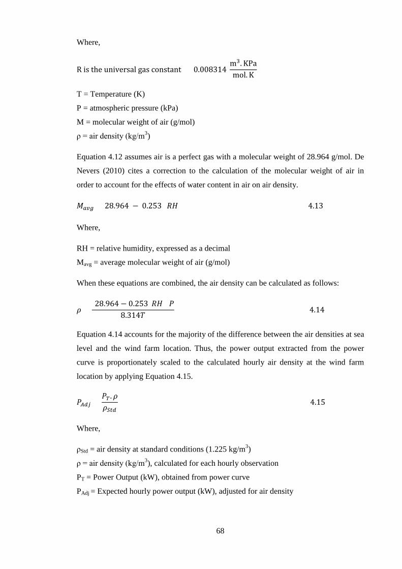
Where,

R is the universal gas constant = 0.008314 m3. KPamol. K

T = Temperature (K)

P = atmospheric pressure (kPa)

M = molecular weight of air (g/mol)

ρ = air density (kg/m3)

Equation 4.12 assumes air is a perfect gas with a molecular weight of 28.964 g/mol. De

Nevers (2010) cites a correction to the calculation of the molecular weight of air in

order to account for the effects of water content in air on air density.

𝑀𝑀𝑎𝑎𝑣𝑣𝑎𝑎 = 28.964 − 0.253 (𝑅𝑅𝑅𝑅) (4.13)

Where,

RH = relative humidity, expressed as a decimal

Mavg = average molecular weight of air (g/mol)

When these equations are combined, the air density can be calculated as follows:

𝜌𝜌 =[28.964 − 0.253(𝑅𝑅𝑅𝑅)]𝑃𝑃

8.314𝑇𝑇 (4.14)

Equation 4.14 accounts for the majority of the difference between the air densities at sea

level and the wind farm location. Thus, the power output extracted from the power

curve is proportionately scaled to the calculated hourly air density at the wind farm

location by applying Equation 4.15.

𝑃𝑃𝐴𝐴𝐴𝐴𝐴𝐴 =𝑃𝑃𝑇𝑇 .𝜌𝜌𝜌𝜌𝐻𝐻𝑡𝑡𝐴𝐴

(4.15)

Where,

ρStd = air density at standard conditions (1.225 kg/m3)

ρ = air density (kg/m3), calculated for each hourly observation

PT = Power Output (kW), obtained from power curve

PAdj = Expected hourly power output (kW), adjusted for air density

68

4.4 Wind Farm Energy Loss Factors

After wind farm design tools have been used to calculate the output of a wind farm, it is

essential to estimate a range of possible sources of energy loss. According to the

European Wind Energy Association (2012), wind farms have six main sources of

energy loss, each of which could be subdivided into more detail. The main loss factors

used to predict net energy output for a wind farm are described below.

Curtailments

All or some of the wind turbines in a wind farm may possibly need to be shut down to

alleviate issues associated with certain planning conditions, turbine loading or export to

the grid.

Environmental

Overtime the surface of the blade may deteriorate or in certain conditions, dirt can form

on the blades. Ice can also build up on a wind turbine. These influences can affect a

wind farms’ energy production. Extremes of weather can also affect the energy

production of a wind farm.

Turbine Performance

In an energy production calculation, a manufacturer supplied power curve is used in the

analysis. Losses need to be assumed however for the inconsistency between actual site

conditions, power curve measurement conditions and losses due to high wind shutdown.

Electrical Efficiency

Electrical losses will be experienced between the low voltage terminals of each of the

wind turbines and the point of connection of the wind farm, which is usually located

within a wind farm switching station.

Availability

The electrical grid and balance of plant infrastructure of wind turbines will not be

available the whole time. As such a factor that accounts for the losses incurred when all

or one of the above inhibits electricity delivery and production needs to be included.

Such losses include grid availability, turbine availability and supporting plant

availability.

69

Wake Effect

When wind turbines extract energy from the wind, there is a wake downstream from the

wind turbine where wind speed is reduced. As the flow proceeds downstream, there is a

scattering of the wake and the wind speed improves towards free stream conditions. The

wake effect is the combined influence on the energy production of the wind farm as a

result of changes in wind speed due to the influence of the turbines on each other.


The guiding principles of wind energy estimation and the main concepts governing

wind farm design are described in this chapter. The chapter discusses the tools used for

estimation of wind farm energy yield, methods for estimating wind characteristics of a

site, and loss factors used to predict net energy output for a wind farm. It draws on the

body of knowledge in wind turbine technology and as a result addresses the unique

challenges associated with wind energy systems and its related processes. This chapter

hence is the basis for the life cycle modelling of the wind farm using the different wind

turbine design options.

70

Chapter 5 Lifecycle Modelling of Wind Farm

This chapter outlines the basic theory behind wind power utilization and illustrates how

the wind farm model used for the comparison was created. A systematic description of

all inputs provided for each model is carried out, specifying all the assumptions made in

order to enable the creation of an accurate onshore wind farm lifecycle model. The wind

farm model is presented to highlight the key differences in modelling requirements. As

such, the wind farm is modelled using the different wind turbine design variations.

5.1 Wind Farm Model

For the purpose of this study, the wind farm created is based on near future and current

trends in wind farm construction projects. In order to build and properly size the model,

existing conditions from a real wind farm was carefully modelled and data at the real

site was used as a reference. As the intention of this investigation is to carry out wind

farm life cycle modelling that meets future and current development expectations, the

establishment of areas for projected future and current wind farm development is the

first step to creating a model. According to information supplied by the British Wind

Energy Association (BWEA, 2015) which chronicles wind projects that have building

permission and accounts for projects that are under construction, Wales has the least of

projected and current wind farm development. This is therefore an indication that Wales

is the least representative area in the British Isles for wind power development. It is also

observed that most of the developments in Wales are concentrated in the south of the

country, bordering the Celtic Sea.

With the establishment of a geographical area of interest, the next step is choosing a

project that represents the nature of prospective wind power developments. After

meticulous consideration of wind farms currently in their construction phase, the Pen y

Cymoedd onshore wind farm, which was given planning consent in May 2012, was

used as the reference wind farm for this study. The wind farm is situated within the

Coed Morgannwg Strategic Search Area, South Glamorgan in Wales, and is projected

to have a maximum installed capacity of 299 MW comprising of 76 wind turbines. The

site is approximately 46.8 km² (as anticipated at the time of consent) (Nuon, 2009). The

actual capacity of the wind farm will depend on the precise turbine manufacturer

selected for the installation. Each turbine will not be less than 2 MW hence the total

minimum capacity will be 168 MW.

71

In the Pen y Cymoedd wind farm Non-Technical Summary (Nuon, 2009), the proposed

construction is set to include four anemometry masts, site tracks, borrow pits,

underground on-site electricity cables and an underground grid connection route, an on-

site 33/132 kilovolt (kV) substation which will house a switchgear and metering

building, construction compounds and associated works/infrastructure. The maximum

dimensions of the wind turbines are also set out at an overall base to tip height not

exceeding 145 metres. The operational life time of the wind farm is expected to be 25

years after which the wind farm will be decommissioned and above ground structures

removed.

The model created for this study includes most aspects of the life cycle of the wind farm

covering construction, operation and decommissioning at the end of the operational

lifetime. In this research, the turbines installed onsite have a 1.5 MW capacity rating.

Thus, the installed capacity of the wind farm will be 114 MW which is less than the

projected wind farm capacity but within the maximum installed capacity of 299 MW.

Table 5-1 summarizes the characteristics of the model wind farm below:

Table 5-1. Wind farm characteristics

Location Pen y Cymoedd, South Wales

Rated Output (MW) 114

Number of turbines 76

Turbine rated Output (MW) 1.5

Project Lifetime (years) 25

The wind regime at the site of the proposed wind farm has to be estimated in order to

calculate the potential farm output. For this to be done, the requirements for providing

accurate energy output estimates and an understanding of how wind power works is

essential. The following sections present a systematic description of how the wind farm

model was setup, as well as information on all the major assumptions.

5.2 Description of the Proposed Site

An assessment of the terrain surrounding the wind farm is an important aspect of any

wind resource analysis. This is essential because surface roughness and elevation

changes are important inputs into the wind flow modelling as well as an indication of

the possible effect that the topography of the surrounding terrain will have on wind

72

turbine performance. It was not possible to carry out analytical wind flow modelling for

the assessment carried out in this study but terrain assessment still influenced wind

speed variation with height estimation as will be seen in the following sections.

Information and map services provided by the British Wind Energy Association

(BWEA, 2015) established the location of the wind farm to be approximately between

the coordinates of 51° 42' 1"N and 3° 37' 27"W as shown in Figure 5-1. The location of

the wind farm can be seen in the satellite image in Figure 5-2 (Google maps, 2014).

From the image, it can be seen that extensive forestry characterizes the area surrounding

the wind farm. The Celtic Sea is to the southwest of the site, which could also influence

wind flow behaviour as it approaches the wind farm from those areas.

Figure 5-1. Location of Pen y Cymoedd wind farm in the U.K

73

Figure 5-2. Surrounding terrain of Pen y Cymoedd wind farm

Low level vegetation in the form of tall grasses, shrubs, and bogs and fens was judged

to constitute the terrain not immediately associated with forestry. Images of the wind

farm site available in the public domain further assisted assessment of the terrain type as

can be seen in Figure 5-3 (StayinWales, 2012; RE News, 2013).

Figure 5-3. Images of Pen y Cymoedd wind farm

74

http://www.google.co.uk/url?sa=i&rct=j&q=&esrc=s&source=images&cd=&cad=rja&uact=8&ved=0CAcQjRxqFQoTCP3Vut-Cn8gCFQpvFAodapkGcA&url=http://renews.biz/45862/earth-to-move-at-pen-y-cymoedd/&psig=AFQjCNH71IG23leIgVcmyUXMa57BXjC9qg&ust=1443711521078767

5.3 Site Wind Resource

A description of the available wind resource at the proposed site is essential for wind

electricity production assessment. For the Pen y Cymoedd wind farm case study, site

specific publicly available information was not obtainable in literature sources to help

estimate the wind resource. This resulted in a search for recorded data at neighbouring

locations which could be modified to generate estimates for the location of the wind

farm. In the UK, the meteorological office has a substantial collection of meteorological

data for several locations across the country (known as the MIDAS Land Surface

Observation Stations Data) through its network of sensors. No wind speed data was

readily available for the exact location of the proposed wind farm but numerous

meteorological stations that could provide information were identified. Three

meteorological stations were found to be available after being filtered for distance (they

were all located within 70 km of the site). The table below summarizes the stations

found.

Table 5-2. Meteorological stations near the proposed wind farm

Met Station Altitude (m) Distance (km) Direction

St Athan 49 31 East

Mumbles Head 43 43 Southwest

Sennybridge No 2 307 66 North

The MIDAS database meteorological data from the meteorological stations contained

consistent hourly averages of wind direction and speed for the period 2005 to 2014 for

all three stations. The MIDAS user guide (United Kingdom Meteorological Office,

2015) states that the standard exposure for all meteorological stations measurements is

over level, open terrain at a 10 m height above the ground. The average mean wind

speed at 10 m was established using this data and is shown below:

Table 5-3. Wind speeds at the meteorological stations

Met station Average Wind Speed (m/s)

St Athan 9.4

Mumbles Head 13.3

Sennybridge No 2 6.8

75

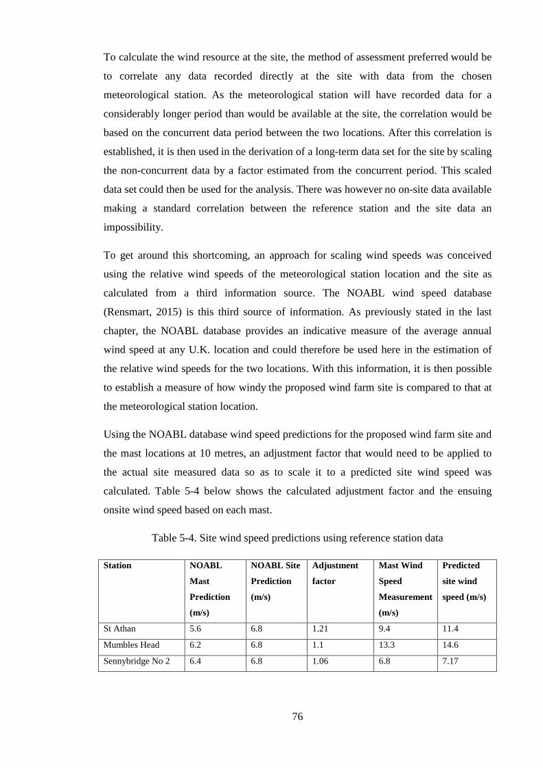
To calculate the wind resource at the site, the method of assessment preferred would be

to correlate any data recorded directly at the site with data from the chosen

meteorological station. As the meteorological station will have recorded data for a

considerably longer period than would be available at the site, the correlation would be

based on the concurrent data period between the two locations. After this correlation is

established, it is then used in the derivation of a long-term data set for the site by scaling

the non-concurrent data by a factor estimated from the concurrent period. This scaled

data set could then be used for the analysis. There was however no on-site data available

making a standard correlation between the reference station and the site data an

impossibility.

To get around this shortcoming, an approach for scaling wind speeds was conceived

using the relative wind speeds of the meteorological station location and the site as

calculated from a third information source. The NOABL wind speed database

(Rensmart, 2015) is this third source of information. As previously stated in the last

chapter, the NOABL database provides an indicative measure of the average annual

wind speed at any U.K. location and could therefore be used here in the estimation of

the relative wind speeds for the two locations. With this information, it is then possible

to establish a measure of how windy the proposed wind farm site is compared to that at

the meteorological station location.

Using the NOABL database wind speed predictions for the proposed wind farm site and

the mast locations at 10 metres, an adjustment factor that would need to be applied to

the actual site measured data so as to scale it to a predicted site wind speed was

calculated. Table 5-4 below shows the calculated adjustment factor and the ensuing

onsite wind speed based on each mast.

Table 5-4. Site wind speed predictions using reference station data

Station NOABL

Mast

Prediction

(m/s)

NOABL Site

Prediction

(m/s)

Adjustment

factor

Mast Wind

Speed

Measurement

(m/s)

Predicted

site wind

speed (m/s)

St Athan 5.6 6.8 1.21 9.4 11.4

Mumbles Head 6.2 6.8 1.1 13.3 14.6

Sennybridge No 2 6.4 6.8 1.06 6.8 7.17

76

The range of predicted site wind speeds shown above prompted a weighted average

approach of the three values that would give the most durable solution. Thus, the

inverse-squared distance method (Shepard, 1968), was used to weigh the above

estimated site wind speeds using the following equation:

𝑉𝑉𝑠𝑠𝑖𝑖𝑡𝑡𝑟𝑟 = 𝑉𝑉1 ×

𝐷𝐷1𝐷𝐷𝑇𝑇�

𝐿𝐿+ 𝑉𝑉2 ×


𝐿𝐿+ 𝑉𝑉3 ×


𝐿𝐿 (5.1)

Where,

𝐿𝐿 = 𝐷𝐷1𝐷𝐷𝑇𝑇

+𝐷𝐷2𝐷𝐷𝑇𝑇

+𝐷𝐷3𝐷𝐷𝑇𝑇

𝐷𝐷𝑇𝑇 = 𝐷𝐷1 + 𝐷𝐷2 + 𝐷𝐷3

𝐷𝐷1−3 = �(𝑥𝑥𝑠𝑠𝑖𝑖𝑡𝑡𝑟𝑟 − 𝑥𝑥1)2 + (𝑦𝑦𝑠𝑠𝑖𝑖𝑡𝑡𝑟𝑟 − 𝑦𝑦1)2

𝑉𝑉1−3 = 𝑓𝑓𝑒𝑒𝑓𝑓𝑒𝑒𝑓𝑓𝑒𝑒𝑛𝑛𝑐𝑐𝑒𝑒 𝑤𝑤𝐵𝐵𝑛𝑛𝑑𝑑 𝐵𝐵𝑝𝑝𝑒𝑒𝑒𝑒𝑑𝑑𝐵𝐵

D1, D2 and D3 = values at the location coordinates of the data points

xsite and ysite = location coordinates of data points at the wind farm site

x1 and y1 = location coordinates of data points at the meteorological station

Using this approach a predicted site wind speed of 11.4 m/s at 10 metres was obtained.

A fundamental limitation of this methodology is the assumption that all the wind

turbines experience the same wind regime i.e. the whole site experiences the same wind

speeds. In cases where turbines are sited in difficult terrain however, this assumption is

inherently flawed and can introduce significant errors in the energy output calculations.

This limitation could be reduced to an extent using the wind flow modelling technique.

For this study, the use of this technique was not possible due to the lack of suitable

modelling capabilities. Figure 5-4 shows the location of the wind farm in relation to the

meteorological stations.

77

Figure 5-4. Location of the meteorological stations and Pen y Cymoedd wind farm

5.4 Hub Height Wind Speed Calculation

The average annual wind speed, as stated in Section 5.3, was estimated from data

recorded at 10 m above ground level. To calculate the energy production of the wind

turbines however, an estimate of the hub height wind speed is required. To determine

this value the Power Law (Equation 4.9) was utilized. The reason for this decision is

because of the lack of accurate data necessary for employing the Log Law and also

because the equations provided a conservative estimate of the wind speed at hub height.

To use the Power Law equation to calculate the shear exponent α, an estimate of the all-

directional average roughness value is necessary. This value is based on an empirical

estimation method, using the site image extending 10 km around the wind farm in all

directions (Troen and Petersen, 1989). The percentage terrain makeup is then

established and weighted using the appropriate roughness classes.

Dividing the area surrounding the wind farm site into 8 segments (of 45 degrees each),

the mix of grassland and woodland was estimated. 87.5% of the segments, from the

northwest to the south, were estimated to be covered by a comfortable percentage of

woodland (60%) and a lesser percentage of agricultural and grass land (40%). For the

outstanding 12.5% of the surrounding area, primarily towards the southwest of the site,

agricultural and grassland constitutes the larger percentage (90%) with woodland far

78

smaller (10%). Based on the roughness classes described in Section 4-2, roughness

values of 0.4 m and 0.03 m were assigned to the woodland and agricultural/grassland

features respectively. Upon calculation of the estimates, they were multiplied with

values using the roughness classes established in Section 4-2.

With the establishment of the all directional roughness value, the shear exponent is

estimated using the equation provided in Gipe (2004):

𝛼𝛼 =1

𝐵𝐵𝑛𝑛 � 𝑧𝑧𝑧𝑧𝑜𝑜�

(5.2)

Where,

z = wind turbine hub height

zo = estimated roughness value

From the equation above, it can be seen that the wind shear is mostly influenced by the

terrain and roughness near the point of measurement. It is noted in Troen and Petersen

(1989) that the wind flow at any location is affected by terrain many metres upwind of

it. The shear exponent was consequently calculated to be 0.19 (for the baseline turbine,

TIO 1 and TIO 3) and 0.17 (for TIO 2 and TIO 4) respectively. According to Gipe

(2004), the shear exponent of flat terrain is around 0.14 thus, the value calculated for the

location of the wind farm is reasonable. Substituting this shear exponent into the Power

Law, the average wind speed at hub height for the baseline turbine, TIO 1 and TIO 3

was calculated to be approximately 16.3 m/s. Average hub height wind speed for TIO 2

and TIO 4 was calculated to be 16.9 m/s.

5.5 Wind Turbine Information

As previously indicated in Chapter 3, for this research the wind farm model is based on

an Enercon E-66 1.5 MW turbine. The turbine’s theoretical power output assumed for

this study is lower than that of the turbine type actually chosen for the wind farm. The

1.5 MW turbine size is currently still in production by most large manufacturers (e.g.

Suzlon, Vestas, Enercon, Nordex, General Electric, Fuhrlander) and continues to be

used worldwide for projects. It is vital to point out that the size and choice of turbine

type is dictated by site-specific as well as economic criteria. However short of a full

analysis of the site, it is unfeasible to precisely decide on the design of the turbine.

Thus, the Enercon E-66 turbine used in this study is assumed to be an acceptable choice

79

for the site. It is however noted that a Siemens 3MW direct drive turbine was selected

for the site in late 2013. A technical summary of the Enercon E-66 1.5 MW turbine is

shown in Table 5-5 below (Papadopoulos, 2010).

Table 5-5. Technical characteristics of E-66 turbine

MODEL: ENERCON E-66

Rated capacity: 1.5 MW

Rotor diameter: 70 m

Hub height: 65 m

Swept area: 3421 m2

Converter concept: gearless, variable speed, variable blade pitch

Rotor with pitch control upwind rotor with active pitch control

Number of blades: 3

Rotor speed: variable, 10 - 22 rpm

Tip speed: 35 – 76 m/s

Pitch control: three synchronized blade pitch systems with emergency supply

Generator: direct-driven ENERCON synchronous ring generator

Grid feeding: ENERCON inverter

Braking system: 3 independent pitch control systems with emergency supply

5.6 Expected Energy Output of the Wind Farm

In order to calculate a wind turbine’s annual energy output in a wind regime, the

approach used was to merge the wind turbine power curve with the wind speed

frequency distribution, hence calculating the energy output at each wind speed interval.

The wind turbine energy output for a year is therefore the sum of these hourly energy

outputs. The power curve used in this research is produced as a consensus power curve

merging the different power curves of three 1.5 MW wind turbines: the Suzlon S.82, the

Nordex S77 and the Fuhrlander FL 1500, as provided by a University of Puerto Rico

study in 2012. Though the consensus power curve is clearly not specific to any

machine, it was taken to represent the standard energy output of a 1.5 MW wind

turbine.

80

Figure 5-5. Consensus power curve for a standard 1.5 MW turbine

It can be seen from the figure above that between 4 m/s and 13 m/s, the power curve

increases and then evens out at 1500 KW until the cut-out speed at 24 m/s. To convert

the power curve to a format that is usable, it was approximated using the 6th order

polynomial equation given below:

y = 0.0006x6 - 0.0584x5 + 2.4372x4 - 50.59x3 + 531.27x2 - 2438.4x + 3945.3 (5.3)

To calculate the energy output of each wind turbine, the power curve is multiplied by

the frequency distribution. The technique used is based on using the Weibull

distribution and the predicted site mean wind speed. For the Weibull distribution, a

shape factor (k) of 2 was chosen (a value that is consistent over northern Europe (Gipe

2004)), and the scale factor (C) was based on the equation C = average hub height wind

speed / 0.9, as given in Patel (2005). The total energy produced by the wind farm is

then estimated by aggregating the energy produced by all the turbines in the wind farm.

Downward corrections then need to be made to account for the losses typical in the

operation of wind farms.

5.6.1 Wind Farm Energy Loss Factors

In this study, six main sources of energy loss are considered; environmental,

curtailments, turbine performance, electrical efficiency, wake effect and availability

with each subdivided into more detailed loss factors as explained in Section 4.4. Table

5-6 summarizes the energy losses assumed for this project.

y = 0.0006x6 - 0.0584x5 + 2.4372x4 - 50.59x3 + 531.27x2 - 2438.4x + 3945.3

R² = 0.9983

0

200

400

600

800

1000

1200

1400

1600

0 5 10 15 20 25

Pow

er O

utpu

t (kw

)

Wind speed (m/s)

81

Table 5-6. Losses assumed for wind farm model (Gipe, 2004)

Production Losses

Curtailments

Wind sector management N/A

Grid curtailment N/A

Noise and visual N/A

Environmental

Performance degradation – non icing N/A

Performance degradation – icing 1%

Icing shutdown 0.2%

Temperature shutdown N/A

Site access N/A

Tree growth (year 1 status assumed) N/A

Turbine Performance

High wind speed hysteresis 0.6%

Site specific power curve adjustment N/A

Electrical efficiency

Operational electrical efficiency 3%

Wind farm consumption 3%

Availability

Turbine availability 2%

Balance of Plant availability 0.2%

Grid availability N/A

Wake effect

Wake effect internal 7%

Total 17%

The specific values used in the above table are based on assumptions given below:

(i) Curtailments

All or some of the turbines within a wind farm may need to be shut down to alleviate

issues associated with export to the grid, certain planning conditions or turbine loading.

a) Wind sector management: Turbine loading is influenced by the wake effects

from nearby turbines. For some wind farms with particularly close turbine

spacing it may be necessary to shut down some turbines for certain wind

conditions. This is referred to as wind sector management and will usually result

in a reduction of the wind farms’ energy production.

82

b) Grid curtailment: Within certain grid connection agreements it may be required

to limit the output of the wind farm at certain times hence, resulting in a loss of

energy production. This factor also includes the time taken for the wind farm to

become fully operational following grid curtailment.

c) Visual, noise, and environmental curtailment: In certain jurisdictions there may

be requirements to shut down turbines during specific meteorological conditions

to meet defined shadow flicker criteria, noise emissions at nearby dwellings, or

environmental conditions due to environmental requirements as regards bats or

birds.

(ii) Environmental

Dirt and ice can form on the wind turbine blades in certain conditions or over time the

surface of the blade may deteriorate. As described in the sections below, these

influences can impact the energy production of a wind farm. The extremes of weather as

well as tree growth and felling can also impact the energy production of a wind farm.

a) Performance degradation – non icing: The performance of wind turbines can be

affected by blade degradation which includes the accumulation of dirt and other

matter, as well as physical degradation due to prolonged operation which

decrease the aerodynamic efficiency of the blades.

b) Performance degradation – icing: Small amounts of icing on the turbine blades

can change the aerodynamic performance of the machine resulting in energy

loss. The factor used in the modelling is based on the assumption made by

Matthies and Aktiengesellschaft (1995).

c) Icing shutdown: As the accumulation of ice gets more severe wind turbines will

shut down. Icing can also affect the wind vane and anemometer on the turbine

nacelle which govern the operations of the turbine. A malfunction of these

instruments can cause a shutdown of the turbine. The factor used in the

modelling is again based on assumptions made by Matthies and

Aktiengesellschaft (1995).

d) Temperature shutdown: Turbines are designed to operate over a specific

temperature range. At certain sites, this range may be exceeded and during the

period when the allowable temperature range is surpassed the turbine will be

shut down.

83

e) Site access: Severe environmental conditions can influence access to more

remote sites which can impact availability. An area prone to severe snow drifts

in the winter is an example of this factor.

f) Felling/tree growth: For wind farm sites located close to or within forestry, the

impact of how the trees may change over time and the effect this will have on

site wind flow and consequently, the energy production of the wind farm must

be considered. This was however deemed outside the scope of this effort.

(iii) Turbine Performance

In an energy production calculation, a power curve provided by the turbine

manufacturer is used within the analysis.

a) High wind hysteresis: Most wind turbines will shut down when the wind speed

exceeds a certain limit. Significant fatigue loading is caused during high wind

speed shut down events. In order to prevent repeated start up and shut down of

the turbine when winds near the shutdown threshold, hysteresis is usually

introduced into the turbine control algorithm. The factor used in this study hence

accounts for the interval in restarting the wind turbine after shutdown and is

based on assumptions made by the European Wind Energy Association.

b) Site specific power curve adjustment: Power curves for wind turbines are

usually based on power curve measurements made on simple terrain test sites.

Certain wind farm sites may experience conditions of wind flow that differ from

conditions seen at terrain test sites. Where it is considered that the parameters in

some areas of a planned wind farm site considerably differ from those at the test

station, the effect on energy production is estimated.

(iv) Electrical efficiency

There will be electrical losses experienced between the low voltage terminals of each of

the wind turbines and the wind farm point of connection, which is generally located

within the switching station of a wind farm.

a) Operational electrical efficiency: This factor defines the electrical losses

experienced when the wind farm is operational and will manifest as a reduction

in the energy measured by an export meter at the point of connection. The factor

used is based on assumptions made by the European Wind Energy Association.

84

b) Wind farm consumption: This factor defines the electrical efficiency due to the

electrical consumption of the non-operational wind farm as a result of

consumption by electrical equipment and transformer no-load losses within the

turbines and substation. The factor used here is based on assumptions made by

Yes2wind (2015).

(v) Availability

Wind turbines, the electrical grid and the “balance of plant” infrastructure will not be

available the whole time over the lifetime of a wind farm. Hence, estimates are included

for likely availability levels for these factors averaged over the lifetime of the project.

a) Turbine availability: This factor defines the expected average turbine availability

of the wind farm over its life time. It represents the factor which needs to be

applied to the gross energy to account for the energy loss associated with the

time the turbines are unavailable for electricity production. The factor assumed

for the modelling is based on Papadopoulos (2010)’s estimate of the availability

of the E-66 wind turbine.

b) Balance of Plant availability: This factor defines the expected availability of the

on-site electrical infrastructure, turbine transformers and the substation

infrastructure up to the point of connection to the grid of the wind farm. It

represents the factor that needs to be applied to the gross energy in order to

account for the energy loss related with the downtime of the balance of plant.

The factor assumed here is taken from Matthies and Aktiengesellschaft (1995).

c) Grid availability: This factor defines the expected grid availability for the wind

farm in mature operation. It also accounts for delays in the wind farm coming

back to full operation following a grid outage. It represents the factor that needs

to be applied to the gross energy to account for energy loss related with the

downtime of the grid connection.

(vi) Wake effect

The wake effect is the aggregated influence on the energy production of a wind farm as

a result of the wind speed changes caused by the impact of the turbines on each other.

The factor used here has been assumed based on information in Nelson (2013).

85

Using the analytical wind data, the assumptions above and assuming 3000 actual load

hours per year, the gross annual energy output of the baseline turbine, TIO 1 and TIO 3

was estimated to be 3.36 GWh/year. For TIO 2 and TIO 4, 3.4 GWh/year was estimated

to be the gross annual energy output for both designs. After estimation of the annual

energy output for the individual turbines, the value was multiplied by the number of

turbines in the wind farm to generate the annual energy output of the wind farm.

Corrections accounting for the losses due to criteria described in Table 5-6 (calculated

to be 17%) was used to modify the estimate for annual output a final time. Based on

these assumptions, the annual energy output of the modelled wind farm (using the

baseline turbine, TIO 1 and TIO 3) was estimated to be 212 GWh/year yielding a

capacity factor of 21%. Modelling the wind farm using TIO 2 and TIO 4, annual energy

output was estimated to be 215 GWh/year with a capacity factor of 22%. These values

are in line with predicted capacity factors for the U.K. as will be seen in the following

section.

5.7 Capacity Factors in the U.K Wind Energy Sector

The capacity factor of a wind turbine in its particular location is another way of stating

the annual energy output from a wind turbine. It is the ratio of the actual output of a

wind energy development to the installed capacity (Oebels and Pacca, 2013). Capacity

factor depends on many parameters, mostly the local wind resource, which in turn

depends on the wind farm location. Thus, capacity factors vary significantly across

countries and regions.

Examination of the evidence supplied by the UK’s onshore wind energy operators to

OFGEM provides an interesting insight. According to Jefferson (2012), the mean

capacity factor achieved by onshore wind farms in England was 22.7% in 2007.

Capacity factors also ranged from 35.09% (Haverigg 3 wind farm), to 24 wind farms

attaining less than a 20% capacity factor (out of 81 operational farms throughout 2007).

Of the latter, six wind farms attained a capacity factor below 10%. Performance was

slightly higher in 2008, as it turned out to be a windier year, with wind farm capacity

factors in Eastern England increasing to 26.2% in 2008 from 22.7% in 2007.

In a report published by Oswald and Ashraf-Ball (2007), a regional analysis of capacity

factors was provided. Given the higher mean wind speeds prevalent in Scotland, it is not

surprising that higher capacity factors have been recorded compared to England. The

average capacity factor in 2006 for southern Scotland was estimated to be 27.6%. The 86

study also highlights capacity factors for the year 2009 as ranging from 15.8% (Isle of

Luig wind farm) up to 48.3% (Barradale Phase 2 wind farm). In 2010, an average

capacity factor of 23.75% was estimated to be achieved in Scotland, indicating a less

windy year compared to 2009.

In Jefferson (2012), Northern Ireland and Wales were noted to turn in lower capacity

factors. The average capacity factor achieved in Wales in 2009 was 23.86% (covering

the performance of 32 wind farms), and 18.75% in 2010 (with 38 wind farms covered).

Three wind farms achieved capacity factors exceeding 30% in 2009 (Moelogen wind

farm being the highest at 33.4%). In 2010, 22 wind farms attained capacity factors

below 20%, nearly two-thirds of all wind farms in Wales. In Northern Ireland 32 wind

farms were reviewed for 2009 and 43 wind farms for 2010. The average capacity factor

achieved in 2009 was 24.1%, and 17.6% in 2010. The Owenreagh wind farm achieved

the highest capacity factor in 2009 (38.2%), with five wind farms achieving more than

30% and nine wind farms achieving under 20%.

As can be seen from the studies above, capacity factors for wind farms in the U.K vary

quite significantly depending on location. It is interesting to note that although wind

farms in Northern Ireland and Wales generally had lower capacity factors compared to

those in England and Scotland, the figures also suggest that annual variations in local

wind resource are too significant to draw any type of conclusion as regards assumptions

about the commercial and technical feasibility of wind farm projects.

5.8 Construction of the Wind Farm

In this section the energy and material inputs required for the construction of the wind

farm model are dealt with. These inputs are based on information collected from

databases as well as external sources as stated in Section 3.5. Each life cycle stage is

split into different components while the assumptions and information sources are

highlighted. The wind farm construction component consists of two inputs: the

“materials” sub-assembly and the “processes” sub-assembly. The “materials” sub-

assembly is a single input covering the different components of the wind turbine, while

the “processes” sub-assembly covers the transportation and energy components required

for construction of the wind farm. Both sub-assemblies are multiplied by a factor of 76,

which is the number of wind turbines that make up the wind farm.

87

5.8.1 Data Source for the 1.5 MW Wind Turbine

As previously mentioned, the turbine model used in this research is an Enercon E-66

three-blade horizontal axis wind turbine. Although this turbine model is not completely

representative of the most recent wind turbine designs, it was chosen for modelling the

wind farm since it conformed to the acceptable wind turbine dimensions as stated in the

Pen y Cymoedd wind farm Non-Technical Summary. Data for the turbine was taken

from a PhD thesis (Papadopoulos, 2010). This source was used in this study to provide a

comprehensive dataset for the E-66 turbine.

5.8.2 Construction of Wind Turbine

Modelling of the Enercon E-66 wind turbine was carried out by splitting it into the

following components shown in Figure 5-5 below:

Figure 5-6. Component breakdown of Enercon E-66

A detailed bill of materials (BOM) for the Enercon E-66 is given in Appendix B: Table

B-1. It should be highlighted that certain assumptions had to be made since the BOM,

though extensive, is not exhaustive. These assumptions are listed in the following

section.

(i) Nacelle

The nacelle houses the control mechanisms and electrical generator that regulate the

directional controls, blade angles and rotation speeds. It is the point of connection for

the nose cone and blades. The nacelle for this turbine model is made up of various steel

compounds with iron constituting the majority of the material mass. It also contains

small amounts of polyester resin, aluminium and copper. The undefined materials were

omitted in the modelling in order not to bias the final results. This of course is presented

88

with the stipulation that no single material in the breakdown of the wind turbine can, on

its own, account for a large percentage of the emission and energy impacts of the unit

modelled.

(ii) Grid Connection and Control Mechanism

This component covers the units necessary to connect the wind turbine to the local

substation, those essential for electricity transmission to the grid, and the control

mechanisms contained in the base and nacelle of the wind turbine. The control

mechanisms are used to position the nacelle for maximum efficiency, as well as adjust

the blades according to the prevalent wind conditions. As a result of the dual nature of

this component it consists of various polymers, light weight concrete and large

quantities of iron and steel. As there was inadequate information about the difference

between certain electronic and electrical components, there was no clear distinction in

the databases of the life-cycle modelling software used. As a result, more generic entries

in the databases were used that covered a range of electrical components.

(iii) Blades

The blades are the major rotary components of the turbine. The major materials

contained in this component are epoxy resin, fibreglass and various plastics. All the

materials were accounted for in the databases used with the exception of a quantity of

material that was undefined. This undefined entry was replaced by iron, on the

assumption that it represented the material requirements for parts such as brackets,

bolts, supports etc. For TIO 1 and TIO 4 (use of stiffer carbon fibre materials allowing

for tower mass reduction as explained in Section 3.4.2.1), Nylon 66/glass fibre

composite (glass-reinforced nylon) was used in the place of fibre glass as it exhibits

similar environmental characteristics to carbon fibre. The databases of the life-cycle

modelling software did not contain information on entries for carbon fibre resulting in

the use of an entry with the closest possible association.

(iv) Tower

The tower supports the main units of the nacelle which include most of the main control

mechanisms, the generator and the blades. It consists mainly of steel and a much lesser

quantity of galvanized steel, and is the component with the largest quantity of these

materials. For TIO 2 and TIO 4 (new tower concepts using carbon fibre materials as

explained in Section 3.4.2.2), glass-reinforced nylon was used in the place of steel due

89

to reasons previously described for the blades. Again, the databases of the life-cycle

modelling software did not contain information on carbon fibre entries hence the use of

the closest possible entry.

(v) Generator

The generator converts the rotational motion of the blades into electrical power. Copper

and steel are the materials that mainly comprise the generator. In the case of TIO 3 (use

of permanent magnets in the generator instead of copper wound rotors as explained in

Section 3.4.2.3.), copper was replaced with iron during entry of the material input into

the life-cycle modelling software. Where materials were undefined, they were omitted

from the model as it was determined that they account for only 1.2% of generator mass

thus there would be minimal impact on the end result.

(vi) Foundation

The foundation provides the base for the tower unit. It mainly consists of concrete and

reinforced steel. As there were no undefined materials, no assumptions were required

for this component.

Table 5-7. Assumptions used in modelling of Enercon E-66 wind turbine and TIOs 1 - 4

Component Assumption Rationale Nacelle Undefined materials omitted To prevent bias of the final

results Grid Connection and Control Mechanism

Generic entries were used to cover range of electrical components

No clear distinction in the difference between electrical components

Blades Undefined material entry replaced by iron For TIO 2 and 4, glass reinforced nylon used in the place of fibre glass

Used to represent material requirements for parts such as brackets, bolts etc. Closest possible entry in SimaPro software to carbon fibre

Tower For TIO 2 and TIO 4, glass reinforced nylon used in the place of steel

Closest possible entry in SimaPro software to carbon fibre

Generator For TIO 3, copper replaced with iron Undefined materials omitted from model

As stated in scenario definition They account for only 1.2% of generator mass

Foundation No assumptions required No undefined materials

90

5.8.3 Energy Requirements for Wind Turbine Manufacture, Assembly and

Dismantling

Chataignere and Boulch (2003) provided data on the energy requirements for the

manufacture, assembly and dismantling of a 1.5 MW wind turbine. It specified the total

primary energy requirement to be 379,734 MJ based on an even split between gas and

electricity. Natural gas inputs were given as 2,625 m3 and electricity requirements given

as 26.3 MWh. The end-of-life of the turbine is assumed to require the same energy

inputs. The “electricity, medium voltage, production RER, at grid/RER U” option of the

Ecoinvent database is the electricity mix considered in order to best represent average

European electricity production.

5.8.4 Site Work

This covers the energy and material requirements during the construction of the wind

farm. Estimates and assumptions had to be made for this section as there was little

available data. The necessary inputs were separated into two categories: inputs related

to component transportation from the manufacturing facilities to the site and the inputs

related to construction work at the site required to make the wind farm operational.

5.8.4.1 Component Transportation

It is necessary to define the likely transportation routes of the components in order to

determine the transportation requirements for construction of the wind farm. As no data

existed describing the exact arrival port for the components, assumptions were made as

regards the most likely route. The components of the wind turbine are assumed to be

transported from the manufacturing facilities in Magdeburg, southern Germany, to

Hamburg port, north Germany. Assumed to be covered by road (40t truck), the distance

is given as 281 km (Google maps, 2014). From Hamburg the components are then

assumed to be transported by container ship to the port of Swansea in Wales, a distance

estimated to be about 1277 km (Google maps, 2014). The components are then

transported by road (40t truck) to their destination at the Pen y Cymoedd wind farm site,

a distance approximated to be 47 km (Google maps, 2014). It should be pointed out that

the foundations are assumed to be sourced locally hence are not included as part of the

components transported from Germany.

91

5.8.4.2 On-site Energy Requirements

For construction on site, the use of heavy machinery is required for the wind farm. For

the purpose of this study, hydraulic diggers (for preparing the foundations of the wind

turbine) and cranes (for erecting the turbines) are assumed to be the main contributors

during site construction. According to Elsam Engineering (2004), each wind turbine

requires the removal of approximately 450m3 of earth. In Rydh et al. (2004), the

installation of a wind turbine is assumed to require approximately 16 hours of crane

work. Chataignere and Boulch (2003) provided data on on-site energy requirements

which was given as 556 MJ. This was used to represent diesel for the building machines

as there were no details about the nature of this input.

5.8.5 Wind Farm Operation

The operation stage of the wind farm encompasses requirements for keeping the wind

farm operational over its lifetime. For the modelling process, some assumptions had to

be made as regards the nature of maintenance to be carried out.

5.8.5.1 Component Replacement

Wear and tear, especially of the rotating components, will occur during operation of the

wind turbines. The lifetime of the wind farm modelled in this study is 25 years. To be

safe, a conservative estimate for maintenance of turbines on the wind farm is assumed

based on assumptions in Vestas (2005). Hence during the lifetime of a wind farm, one

renewal of half of the generators or the gearboxes must be carried out which is expected

to, as a minimum, comprise renewal of the bearings. For the purpose of this study, this

assumption was simplified to be a total renewal of half of the generators once in the

lifetime of the wind farm.

5.8.5.2 Oils and Lubricants

According to D’Souza et al. (2011), wind turbines require a replacement of lubricant

and oils on a regular basis. In this study two assumptions are made based on data in

Rydh et al. (2004) and Vestas (2005). Both studies state that each wind turbine requires

320 litres of gear oil for every 5 years of operation and the lubrication requirements for

each wind turbine is 16 kg per year.

92

5.8.5.3 Inspection and Maintenance

The use of a hydraulic crane was added to the modelling process to simulate the actual

inspection procedure. To replace the generators, the assumption in Rydh et al. (2004)

that each turbine required crane use for 8 hours was used. Inspection requirements were

also based on Rydh et al. (2004)’s assumption that every 6 months, a passenger car

would inspect the site. The distance travelled for the inspection procedure is assumed to

be 120 km based on a round trip from the operations base to the wind farm.

5.8.6 Wind Farm Decommissioning

There is insufficient information about this life cycle stage of wind farms as few wind

farms have actually been decommissioned up to now. There is however data on the

theoretical disposal of wind turbines to enable the modelling of this stage. The turbines

are assumed to be disassembled using a mobile crane and transported 500 km by road

(40t truck) to a disposal facility. Energy requirements for dismantling at the facility are

assumed to be 2,625 m3 of natural gas and 26.3 MWh of electricity as stated in Section

5.8.3. The foundations of the turbines are assumed to be left behind on the wind farm

site. As already shown in Figure 3-3, the influence of disposing/recycling components

of the wind farm was not included in this study.

5.8.7 Cut-off criteria

The cut-off criteria given below were used to make certain that all relevant possible

environmental impacts were represented:

• Energy - if a flow is less than 1% of the energy at a product-level, then it may

be excluded, provided its environmental relevance is not a concern.

• Mass - if a flow is less than 1% of the mass at a product-level, then it may be

excluded, provided its environmental relevance is not of concern.

• Environmental relevance - if a flow meets the above exclusion criteria, but is

considered to possibly have a significant environmental impact, it should be

included. All material flows leaving the system (emissions) and whose

environmental impact is higher than 1% of the whole impact of an impact

category that has been considered in the assessment, should be included.

• The sum of the neglected material flows should not exceed 5% of total energy,

mass or environmental relevance, at a product-level.

93


The previous sections have shown the methods employed to create the model for the

wind farm. Thus it can be seen that despite the differences in the turbine design

variations, similar modelling approaches were adopted. In all cases however where

assumptions and approximations were altered, they have been specified to ensure

clarity.

Due to the potential for technological advancements to reduce the cost and increase the

performance of wind turbines, as stated in Section 3.4.2, their design is a matter of

continuous compromise between rival demands. This necessity has had a direct impact

on the potential TIOs employed in the wind turbine models. As a result, different

scaling relationships and procedures were required to model each design variation while

the energy and material inputs did not require specific data collection. Equally, the lack

of comprehensive site measurements for the wind farm resulted in the use of a scaling

method utilizing data from nearby meteorological stations.

The subsequent models are however believed to reflect conditions at the wind farm site

and therefore provide a good basis for computations of the wind power lifecycle using

the different design variations.

94

Chapter 6 Results and Discussion

This chapter presents the results of the integrated methodology, outlined in Chapter 3,

for the different wind turbine design variations and wind farm models developed. The

chapter is organized such that for each methodological tool used in the assessment, the

performance of each design variation is assessed and then compared to the others. The

chapter starts in Section 6.1 with a presentation and discussion of the results for the

uncertainty analysis as this was conducted for a single wind turbine. This is followed by

presentation and discussion of results for the wind farm lifecycle using the different

design variations in Section 6.2. Finally, Section 6.3 presents and discusses the

economics as regards the use of each design variation on the wind farm.

6.1 Uncertainty Analysis

This section addresses the data uncertainty quantification aspect of the sustainability

assessment. Estimation of the embodied energy and embodied carbon for the different

wind turbine design variations was performed. The composition of materials data for the

baseline turbine and TIOs 1 - 4, presented in Appendix A: Tables A-1 to A-5, formed

the basis for deterministic estimation of the embodied energy and embodied carbon.

Since the material quantities were taken from the same source, they have little or no

variations. The deterministic result estimate (Appendix A: Table A-6) is used as a point

of reference for comparing outputs of the stochastic estimation. The results are

presented and discussed in the sections below.

6.1.1 Quantitative DQI Transformation

To appropriately transform the qualitative assessment results to the equivalent

quantitative probability density functions, Wang and Shen (2013) suggests that the

aggregated DQI scores be approximated to the nearest nominal value so as to use the

transformation matrix. Table 6-1 shows the obtained aggregated DQI scores, for the

baseline turbine, following the method described in Section 3.6.2.1. The quantitative

DQI procedure was then used to transform the scores into Beta distributions, results of

which are shown in Table 6-1. Most of the data used in the study are of good quality

and were taken from the same data source and hence showed identical transformed Beta

function parameters (α = 4, β = 4), the same DQI score of 4.5 and range end points of ±

15%. The exceptions were Cast iron EF, Cast iron EEC and Gear oil EEC showing DQI

95

scores of 3.5, transformed Beta function parameters of (α = 2, β = 2) and range end

points of ± 25% making them more uncertain.

Table 6-1. Transformation of DQI scores to probability density functions

EF Parameters Beta (α, β)

Range endpoints

EEC Parameters Beta (α, β)

Range endpoints

Aluminium (EF) (4, 4) (+/-15%) ≈ (1.7, 2.3)

Aluminium (EEC) (4, 4) (+/-15%) ≈ (131.8, 178.3)

Fibre glass (EF) (4, 4) (+/-15%) ≈ (6.9, 9.3)

Fibre glass (EEC) (4, 4) (+/-15%) ≈ (85, 115)

Epoxy resin (EF) (4, 4) (+/-15%) ≈ (5, 6.8)

Epoxy resin (EEC) (4, 4) (+/-15%) ≈ (118, 160)

Polyethene (EF) (4, 4) (+/-15%) ≈ (1.7, 2.2)

Polyethene (EEC) (4, 4) (+/-15%) ≈ (70.6, 95.6)

PVC (EF) (4, 4) (+/-15%) ≈ (2.1, 2.8)

PVC (EEC) (4, 4) (+/-15%) ≈ (65.6, 88.8)

Paint (EF) (4, 4) (+/-15%) ≈ (3, 4.1)

Paint (EEC) (4, 4) (+/-15%) ≈ (57.8, 78.2)

Rubber (EF) (4, 4) (+/-15%) ≈ (2.7, 3.7)

Rubber (EEC) (4, 4) (+/-15%) ≈ (86.4, 117)

Iron (EF) (4, 4) (+/-15%) ≈ (1.6, 2.2)

Iron (EEC) (4, 4) (+/-15%) ≈ (21.3, 28.8)

Steel (EF) (4, 4) (+/-15%) ≈ (2.3, 3.2)

Steel (EEC) (4, 4) (+/-15%) ≈ (20.7, 28)

Galvanized steel (EF)

(4, 4) (+/-15%) ≈ (2.4, 3.2)

Galvanized steel (EEC)

(4, 4) (+/-15%) ≈ (33.2, 45)

Copper (EF) (4, 4) (+/-15%) ≈ (3.3, 4.4)

Copper (EEC) (4, 4) (+/-15%) ≈ (42.5, 57.5)

Steel sheet (EF) (4, 4) (+/-15%) ≈ (2.1, 2.9)

Steel sheet (EEC) (4, 4) (+/-15%) ≈ (27, 36.2)

Steel (no alloy) (EF)

(4, 4) (+/-15%) ≈ (1.5, 2)

Steel (no alloy) (EEC)

(4, 4) (+/-15%) ≈ (29.2, 39.6)

Steel (alloy, high grade) (EF)

(4, 4) (+/-15%) ≈ (2.4, 3.2)

Steel (alloy, high grade) (EEC)

(4, 4) (+/-15%) ≈ (48.2, 65.2)

Steel (alloy, low grade) (EF)

(4, 4) (+/-15%) ≈ (2.3, 3.1)

Steel (alloy, low grade) (EEC)

(4, 4) (+/-15%) ≈ (41, 55.7)

Cast Steel (EF) (4, 4) (+/-15%) ≈ (2.4, 3.3)

Cast Steel (EEC) (4, 4) (+/-15%) ≈ (21.6, 29.2)

Cast iron (EF) (2, 2) (+/-25%) ≈ (1.4, 2.4)

Cast iron (EEC) (2, 2) (+/-25%) ≈ (19.5, 32.5)

Unsaturated polyester resin (EF)

(4, 4) (+/-15%) ≈ (1.7, 2.2)

Unsaturated polyester resin (EEC)

(4, 4) (+/-15%) ≈ (96.1, 130)

Electronics (EF) (4, 4) (+/-15%) ≈ (2.3, 3.1)

Electronics (EEC) (4, 4) (+/-15%) ≈ (68.4, 92.6)

Steel (for construction) (EF)

(4, 4) (+/-15%) ≈ (0.6, 0.8)

Steel (for construction) (EEC)

(4, 4) (+/-15%) ≈ (30.6, 41.4)

Gear oil (EF) (4, 4) (+/-15%) ≈ (3.1, 4.2)

Gear oil (EEC) (2, 2) (+/-25%) ≈ (41.3, 69)

Light weight concrete (EF)

(4, 4) (+/-15%) ≈ (0.1, 0.2)

Light weight concrete (EEC)

(4, 4) (+/-15%) ≈ (0.7, 0.9)

Normal concrete (EF)

(4, 4) (+/-15%) ≈ (0.17, 0.23)

Normal concrete (EEC)

(4, 4) (+/-15%) ≈ (1.2, 1.6)

96

Figure 6-1. Aggregated DQI scores for emission factors and embodied energy

coefficients

6.1.2 Parameter Categorization and Probability Distributions Estimation

Results of the influence analysis (10,000 iterations MCS) showing the two parameters

contributing the most to the resulting uncertainty is presented in Table 6-2. Two

parameters, Steel and Carbon fibre reinforced plastic (CFRP), demonstrated the largest

influence on the final resulting uncertainty of embodied energy and embodied carbon

across all case studies. For the parameters with a lesser contribution to the final

resulting uncertainty, there were variations across all case studies. Normal concrete and

CFRP show the lesser contribution for embodied carbon, while Steel (no alloy), CFRP

and Cast iron show the lesser contribution for embodied energy across all case studies.

Combining these results, further analysis was conducted on the two identified

parameters for each test case using the statistical method, while the values for the

remaining parameters were obtained from the quantitative DQI. Probability

distributions were thus fitted to data points collected manually from literature. Results

of the estimated probability distributions for the different parameters are presented in

Table 6-3.

3

3.5

4

4.5

5

DQ

I sco

res o

f EF'

s and

EE

C's

Materials

EF's EEC's

97

Table 6-2. Influence Analysis

Embodied Carbon Influence (%) Embodied Energy Influence (%) Baseline Turbine

Steel EF 78 Steel EEC 62 Normal concrete EF 9 Steel (no alloy) EEC 9

TIO 1 Steel EF 66 Steel EEC 47 CFRP EF 17 CFRP EEC 22

TIO 2 CFRP EF 99 CFRP EEC 97 Normal concrete EF 0.3 Steel (no alloy) EEC 0.7

TIO 3 Steel EF 81 Steel EEC 66 Normal concrete EF 8 Cast iron EEC 9

TIO 4 CFRP EF 98 CFRP EEC 97 Normal concrete EF 0.6 Steel (no alloy) EEC 0.5

Table 6-3. Probability distribution estimation for the different parameters

Parameter Probability Distribution

Mean Data points collected

Source

Steel EF Steel EEC

Beta (1.24, 4.47) Beta (2.96, 4.16)

1.73 tonCO2/ton 25.87 GJ/ton

30 31

Hammond and Jones, 2008; Fleck and Huot, 2009; Alcorn and Wood, 1998; Norgate et al., 2007; Rankine et al., 2006; Khan et al., 2005; Change, 2006; Hammond and Jones, 2011; Lee et al., 2011; Baird et al., 1997

Normal concrete EF

Beta (20.8, 87.7)

0.11 tonCO2/ton

31 Hammond and Jones, 2008; Hammond and Jones, 2011; Alcorn and Wood, 1998; Norgate et al., 2007; Rankine et al., 2006

Steel (no alloy) EEC

Beta (48.6, 62.3)

25.57 GJ/ton 31 Hammond and Jones, 2008; Alcorn and Wood, 1998; Norgate et al., 2007; Rankine et al., 2006; Khan et al., 2005; Change, 2006; Lee et al., 2011; Baird et al., 1997; Fernando, 2010

CFRP EF CFRP EEC

Beta (3.16, 2.2) Beta (2.13, 6.23)

52.4 tonCO2/ton 191.3 GJ/ton

31 31

Hill et al., 2011; Kirihara et al., 2011; Pimenta and Pinho, 2011; Howarth et al., 2014; Douglas et al., 2008; Song et al., 2009; Rydh and Sun, 2005; Duflou et al., 2012

Cast iron EEC

Beta (36.6, 75.2)

35.4 GJ/ton 31 Fernando, 2010; Du et al., 2012; TERI, 2012; Hendrickson and Horvath, 2014; Sharma et al., 2013; Baum et al., 2009; Sefeedpari et al., 2012; Lenzen and Dey, 2000; Lenzen and Treloar, 2002; Baird et al., 1997

98

6.1.3 Stochastic Results Comparison of DQI and HDS Approaches for the

Different Case Studies

Embodied carbon and embodied energy stochastic results (10,000 iterations MCS) using

the pure DQI and HDS methods were obtained for the baseline turbine and TIO’s 1 - 4

the results of which are presented in this section. Results for each case study are

presented graphically through probability distribution functions (PDF’s) and cumulative

distribution functions (CDF’s) in Figures 6-2 to 6-11. In addition to these figures, MRE

and CV values were also calculated. A summary of the relevant information is provided

in Table 6-4.

Table 6-4. Pure DQI and HDS results for the different case studies

Embodied Carbon Embodied Energy

DQI HDS DQI HDS Baseline Turbine Beta distribution

(4.5, 5.3) μ = 932 tonCO2 σ = 22 tonCO2 CV = 0.02

Beta distribution (1.8, 5.1) μ = 733 tonCO2 σ = 183 tonCO2 CV = 0.25 MRE = 27%

Normal distribution μ = 11909 GJ σ =218 GJ CV = 0.02

Beta distribution (4.4, 4.7) μ = 11831 GJ σ = 1424 GJ CV = 0.12 MRE = 1%

TIO 1 Normal distribution μ =1070 tonCO2 σ = 24 tonCO2 CV = 0.02

Beta distribution (2.3, 5.2) μ =1269 tonCO2 σ =188 tonCO2 CV = 0.15 MRE = 16%

Normal distribution μ = 13735 GJ σ = 244 GJ CV = 0.02

Beta distribution (3.8, 4.7) μ = 13276 GJ σ = 1469 GJ CV = 0.11 MRE = 3.5%

TIO 2 Beta distribution (5, 5.3) μ = 2475 tonCO2 σ = 96 tonCO2 CV = 0.04

Beta distribution (5.8, 4.1) μ = 5521 tonCO2 σ = 1654 tonCO2 CV = 0.3 MRE = 55%

Beta distribution (4.1, 4.8) μ = 31822 GJ σ = 1166 GJ CV = 0.04

Beta distribution (2.4, 4.7) μ =24687 GJ σ = 7608 GJ CV = 0.3 MRE = 29%

TIO 3 Beta distribution (5.3, 5.7) μ = 849 tonCO2 σ = 22 tonCO2 CV = 0.03

Beta distribution (1.6, 4.6) μ = 647 tonCO2 σ =185 tonCO2 CV = 0.29 MRE = 31%

Normal distribution μ =10722 GJ σ =211 GJ CV = 0.02

Beta distribution (3.8, 4.8) μ =11249 GJ σ = 1474 GJ CV = 0.13 MRE = 5%

TIO 4 Gamma distribution (529, 4.8) μ = 2529 tonCO2 σ = 108 tonCO2 CV = 0.04

Weibull distribution (3.96, 6621) μ = 5988 tonCO2 σ = 1746 tonCO2 CV = 0.29 MRE = 58%

Beta distribution (4.7, 4.5) μ = 32503 GJ σ = 1304 GJ CV = 0.04

Beta distribution (2.1, 4.6) μ = 24299 GJ σ = 8419 GJ CV = 0.35 MRE = 33%

99

6.1.3.1 Baseline Turbine

Figures 6-2 and 6-3 show the stochastic results (10,000 runs MCS) for embodied carbon

and embodied energy using the HDS and DQI methods. For embodied carbon, Beta

distribution (4.5, 5.3) was fitted, according to K-S test, to the DQI result with a mean

value of 932 tonCO2 and a standard deviation of 22 tonCO2. The HDS follows Beta

distribution (1.8, 5.1) (K-S test), with a mean value of 733 tonCO2 and standard

deviation of 183 tonCO2 thus having a larger spread compared to the DQI result. The

CV value of the HDS result is 0.25, 1250% larger than the DQI result CV value of 0.02.

The (10%, 90%) certainty interval for the output of the DQI result is (904 tonCO2, 960

tonCO2) with a span of 56 tonCO2, while the HDS presents a much greater (10%, 90%)

certainty interval of (535 tonCO2, 992 tonCO2) with a span of 458 tonCO2. In terms of

MRE, a 27% difference was observed between the HDS and pure DQI results showing

that the HDS approach captured more possible outcomes compared to the pure DQI.

The differences in the results can also be deduced from the CDF (Figure 6-2b). For the

HDS result, about 85% of the likely results are smaller than the obtained deterministic

result while for the DQI result, 50% of the likely resulting values are smaller than the

obtained deterministic result.

For embodied energy, Normal distribution with a mean value of 11909 GJ and standard

deviation of 218 GJ was fitted, according to K-S test, to the DQI result. The HDS result

follows Beta distribution (4.4, 4.7) (K-S test), with a mean value of 11831 GJ and

standard deviation of 1424 GJ. The CV value of the HDS result is 0.12 compared to

0.02 for the pure DQI result. The (10%, 90%) certainty interval for the HDS output is

(9918 GJ, 13799 GJ) with a span of 3880 GJ while the (10%, 90%) certainty interval for

the DQI output is (11625 GJ, 12187 GJ) with a span of 562 GJ. For the MRE, a 1%

difference was observed between the DQI and HDS results. The CDF (Figure 6-3b)

shows half of the likely resulting values are smaller than the obtained deterministic

result for both the DQI and HDS results.

100

Figure 6-2. (a) Baseline Turbine Embodied Carbon PDF results; (b) Baseline Turbine

Embodied Carbon CDF results

101

Figure 6-3. (a) Baseline Turbine Embodied Energy PDF results; (b) Baseline Turbine

Embodied Energy CDF results

102

6.1.3.2 TIO 1

For embodied carbon, a Normal distribution with mean value of 1070 tonCO2 and

standard deviation of 24 tonCO2 (K-S test) was fitted to the DQI result. Beta


deviation of 188 tonCO2 was fitted to the HDS result thus having a larger dispersion

compared to the DQI result. The CV value of the HDS result is 0.15, which is larger

than the DQI result CV value of 0.02. The (10%, 90%) certainty interval for the output

of the DQI result is (1037 tonCO2, 1101 tonCO2) with a span of 64 tonCO2, while the

HDS presents a much greater (10%, 90%) certainty interval of (1066 tonCO2, 1565

tonCO2) with a span of 500 tonCO2. In terms of MRE, a difference of 16% was

observed between the HDS and pure DQI results. It is seen from the CDF (Figure 6-4b)

that for the HDS result, about 15% of the possible results are smaller than the obtained

deterministic result. While for the DQI result, 50% of the possible resulting values are

smaller than the obtained deterministic result.

For the embodied energy, a Normal distribution with mean value of 13735 GJ and

standard deviation of 244 GJ (K-S test) was fitted to the DQI result. The HDS result




(11345 GJ, 15333 GJ) with a span of 3988 GJ while the (10%, 90%) certainty interval

for the DQI output is (13407 GJ, 14058 GJ) with a span of 652 GJ. For the MRE, a

3.5% difference was observed between the DQI and HDS results. The CDF (Figure 6-

5b) shows that for the HDS result about 60% of the possible results are smaller than the

obtained deterministic result while for the DQI result, 50% of the possible resulting

values are smaller than the obtained deterministic result.

103


results

104


results

105

6.1.3.3 TIO 2

For embodied carbon, Beta distribution (5, 5.3) (K-S test), with a mean value of 2475

tonCO2 and standard deviation of 96 tonCO2 was fitted to the DQI result. Beta


deviation of 1654 tonCO2 was fitted to the HDS result thus having a larger dispersion

than the DQI result. The CV value of the HDS result is 0.3, which is larger than the DQI

result CV value of 0.04. The (10%, 90%) certainty interval for the output of the DQI

result is (2345 tonCO2, 2606 tonCO2) with a span of 261 tonCO2, while the HDS

presents a much larger (10%, 90%) certainty interval of (3153 tonCO2, 7722 tonCO2)

with a span of 4568 tonCO2. In terms of MRE, a 55% difference was observed between

the HDS and pure DQI results. It is seen from the CDF (Figure 6-6b) that for the HDS

result, about 0.01% of the likely results are smaller than the obtained deterministic

result. While for the DQI result, 50% of the likely resulting values are smaller than the


For the embodied energy, Beta distribution (4.1, 4.8) (K-S test), with mean value of

31822 GJ and standard deviation of 1166 GJ was fitted to the DQI result. The HDS

result follows Beta distribution (2.4, 4.7) (K-S test), with a mean value of 24687 GJ and

standard deviation of 7608 GJ. The CV value of the HDS result is 0.3 compared to 0.04

for the pure DQI result. The (10%, 90%) certainty interval for the HDS output is (15704

GJ, 35845 GJ) with a span of 20141 GJ while the (10%, 90%) certainty interval for the

DQI output is (30231 GJ, 33399 GJ) with a span of 3169 GJ. For the MRE, a 29%

difference was observed between the DQI and HDS results. For the HDS result the CDF

(Figure 6-7b) shows about 85% of the possible results are smaller than the obtained

deterministic result while for the DQI result, half of the possible resulting values are

smaller than the obtained deterministic result.

106


results

107


results

108

6.1.3.4 TIO 3

For embodied carbon Beta distribution (5.3, 5.7) was fitted, according to K-S test, to the

DQI result with a mean value of 849 tonCO2 and a standard deviation of 22 tonCO2.

The HDS follows Beta distribution (1.6, 4.6) (K-S test), with a mean value of 647

tonCO2 and standard deviation of 185 tonCO2 thus having a larger dispersion compared

to the DQI result. The CV value of the HDS result is 0.3, which is larger than the DQI

result CV value of 0.03. The (10%, 90%) certainty interval for the output of the DQI

result is (820 tonCO2, 878 tonCO2) with a span of 58 tonCO2, while the HDS presents a

much larger (10%, 90%) certainty interval of (454 tonCO2, 920 tonCO2) with a span of

467 tonCO2. In terms of MRE, a 31% difference was observed between the HDS and

pure DQI results. It is seen from the CDF (Figure 6-8b) that for the HDS result, about

85% of the possible results are smaller than the obtained deterministic result. While for

the DQI result, 50% of the possible resulting values are smaller than the obtained

deterministic result.

For the embodied energy, a Normal distribution with mean value of 10722 GJ and

standard deviation of 211 GJ (K-S test) was fitted to the DQI result. The HDS result




(9268 GJ, 13346 GJ) with a span of 4078 GJ while the (10%, 90%) certainty interval for

the DQI output is (10457 GJ, 10986 GJ) with a span of 529 GJ. For the MRE, a 5%

difference was observed between the DQI and HDS results. The CDF (Figure 6-9b)

shows about 35% of the possible results are smaller than the obtained deterministic

result while for the DQI result, half of the possible resulting values are smaller than the


109


results

110


results

111

6.1.3.5 TIO 4

Results for the embodied carbon show Gamma distribution (529, 4.8) was best fitted,

according to K-S test, to the DQI result with a mean value of 2529 tonCO2 and a

standard deviation of 108 tonCO2. The HDS follows Weibull distribution (3.96, 6621)

(K-S test), with a mean value of 5988 tonCO2 and standard deviation of 1746 tonCO2.

The CV value of the HDS result is 0.29, which is larger than the DQI result CV value of

0.04. The (10%, 90%) certainty interval for the output of the DQI result is (2381

tonCO2, 2671 tonCO2) with a span of 289 tonCO2, while the HDS presents a much

greater (10%, 90%) certainty interval of (3599 tonCO2, 8245 tonCO2) with a span of

4646 tonCO2. In terms of MRE, a 58% difference was observed between the HDS and

pure DQI results. It is seen from the CDF (Figure 6-10b) that for the HDS result, about

0.01% of the possible results are smaller than the obtained deterministic result. For the

DQI result, 50% of the possible resulting values are smaller than the obtained

deterministic result.

Results for the embodied energy show Beta distribution (4.7, 4.5) was best fitted,

according to K-S test, to the DQI result with a mean value of 32503 GJ and a standard

deviation of 1304 GJ. The HDS result follows Beta distribution (2.1, 4.6) (K-S test),

with a mean value of 24299 GJ and standard deviation of 8419 GJ. The CV value of the

HDS result is 0.35 compared to 0.04 for the pure DQI result. The (10%, 90%) certainty

interval for the HDS output is (14097 GJ, 36263 GJ) with a span of 22165 GJ while the

(10%, 90%) certainty interval for the DQI output is (30725 GJ, 34283 GJ) with a span

of 3558 GJ. For the MRE, a 33% difference was observed between the DQI and HDS

results. The CDF (Figure 6-11b) shows about 85% of the possible results are smaller

than the obtained deterministic result while for the DQI result, half of the possible

resulting values are smaller than the obtained deterministic result.

112

Figure 6-10. (a) TIO 4 Embodied Carbon PDF results; (b) TIO 4 Embodied Carbon

CDF results

113

Figure 6-11. (a) TIO 4 Embodied Energy PDF results; (b) TIO 4 Embodied Energy

CDF results

114

6.1.4 Comparison of Statistical and HDS Methods in terms of Data Requirements

It can be seen that from the procedure of the HDS approach which categorizes critical

parameters and uses the statistical method to estimate their probability distributions, the

HDS approach captures more possible outcomes compared to the DQI. According to

Wang and Shen (2013), the statistical method requires at least 30 data points to estimate

one parameter distribution. Hence in this study, 46 parameter distributions are required

to be estimated for each case study with the exception of TIO 1 which has 48 parameter

distributions for estimation. If the statistical method was implemented, at least 1380

data points would have been required for the estimation for each case study. That would

mean 6900 data points across all the case studies. This would have been very time

consuming even if all the data points were available. The HDS requires only 120 data

points for each case study (600 data points across all the case studies) thus reducing the

data requirements by approximately 91%. This avoids the issue associated with lack of

data, and saves cost and time without seriously compromising the reliability of the HDS

results as the critical parameters identified explain the majority (at least 69%) of the

overall uncertainty across all the case studies.

6.1.5 Discussion

The HDS approach is used to provide insight into potential technological advancements

for a 1.5 MW wind turbine and makes evident how variability of input parameters

culminates in differing embodied energy and embodied carbon results. Analysing the

parameter categorization revealed that EF’s and EEC’s for Steel, Normal concrete, Steel

(no alloy), CFRP and Cast iron accounted for the majority of output uncertainty in

embodied energy and embodied carbon results. Steel is the main material component of

the baseline wind turbine, followed by normal concrete. The large contribution of steel

is probably attributed to the wide EF and EEC distributions assigned to steel in the

probability distribution estimations. Therefore any uncertainty in steel EF’s and EEC’s

is magnified by the sheer mass of steel. Interestingly although the mass of concrete (575

tons) is greater than the mass of steel (144 tons), steel EF’s and EEC’s contribute more

to the overall uncertainty of embodied energy and embodied carbon. For example, the

EF’s of steel ranges from 0.01 – 5.93 tonCO2/ton steel, whereas values for concrete

range from 0.02 – 0.28 tonCO2/ton. Likewise, the EEC’s for steel range from 8.6 – 51

GJ/ton steel, whereas values for steel (no alloy) range from 8.3 – 50.7 GJ/ton. Concrete

generally is much less emission intensive than steel for CO2 and hence, is a lesser

115

contributor to the sensitivity of embodied carbon. It can also be observed that while

normal concrete EF and steel (no alloy) EEC contribute 9% each, steel EF and steel

EEC contribute 78% and 62% respectively to the resulting uncertainty. This highlights

the influence of the wider distribution range of steel (no alloy) EEC compared to normal

concrete EF. Due to the wide distribution ranges and mass of steel, variations in steel

EF’s and EEC’s have significantly more impact on the embodied energy and embodied

carbon uncertainty even though there is normally more concrete than steel.

For TIO 1, normal concrete and steel are also major material components of the turbine

with 575 tons and 141 tons respectively. However CFRP contributes considerably to the

resulting uncertainty, second only to steel, while having a mass of 8.6 tons (1% of the

turbine mass). This can be attributed to CFRP being very emission and energy intensive.

The EF’s for CFRP range from 11.2 – 86.3 tonCO2/ton CFRP, compared to the steel EF

range of 0.01 – 5.93 tonCO2/ton steel. Similarly, the EEC’s for CFRP range from 55 –

594 GJ/ton CFRP compared to the steel EEC range of 8.6 – 51 GJ/ton steel. Hence due

to the wide distribution ranges in CFRP EF and EEC input factors, despite its minor

mass contribution, CFRP has a considerable impact on the uncertainty of the embodied

energy and embodied carbon. For TIO 2, the major material components are normal

concrete and CFRP with 575 tons and 88.5 tons respectively. Despite being second in

mass to steel, CFRP contributes 99% and 97% of the resulting uncertainty for embodied

carbon and embodied energy respectively. This is attributed to its high emission

intensity, energy intensity and wide distribution ranges. As a result, CFRP significantly

impacts the uncertainty of the embodied energy and embodied carbon.

Normal concrete and steel are the major material components in TIO 3 with 575 and

144 tons respectively. The contribution of steel to the final resulting uncertainty is again

attributed to the range of values of EF’s and EEC’s. Cast iron has a mass of 21 tons and

EEC values ranging between 11.7 – 94.5 GJ/ton which could explain the lesser

contribution of steel EEC to the resulting uncertainty for the embodied energy (66%)

compared to the steel EF contribution for embodied carbon (81%). For TIO 4, the major

material components are normal concrete with 575 tons and CFRP with 97 tons. CFRP

contributes 98% and 97% of the resulting uncertainty for embodied carbon and

embodied energy respectively. Again the sheer tonnage of CFRP combined with its high

emission and energy intensity, and wide distribution ranges results in its significant

contribution to the resulting uncertainty of the embodied energy and embodied carbon.

116

The intention of quantifying uncertainty with the HDS approach in this study is to

provide more information for the decision making process. From the above case studies,

it is assumed that the deterministic result is used for design scheme selection aiming to

find an embodied carbon and embodied energy saving design. The baseline turbine is

commercially available hence in terms of embodied carbon, there is an about 85%

probability (Fig. 6-2b) Enercon saved carbon emissions with the design. Thus, it is a

good design in terms of embodied carbon savings. In terms of embodied energy there is

a 50% probability (Fig. 6-3b) Enercon reduced the primary energy consumed during

manufacture with the design. The TIO’s proposed in this study are design concepts.

Hence for TIO 1 in terms of embodied carbon, there is an about 15% probability (Fig.

6-4b) that a manufacturer will be able to reduce carbon emissions with this design.

Hence, it is not a good design for embodied carbon savings. In terms of embodied

energy, there will be a 60% (Fig. 6-5b) probability that a manufacturer will be able to

reduce the primary energy consumed. This design thus performs better in terms of

embodied energy savings.

For TIO 2 results show that for embodied carbon, there is a 1% probability (Fig. 6-6b) a

manufacturer will be able to reduce carbon emissions therefore making it a bad design.

The embodied energy results show that there is about an 85% probability (Fig. 6-7b) a

manufacturer will be able to reduce the primary energy consumed making it a good

design in terms of embodied energy savings. The huge difference in the results, despite

CFRP’s contribution of 99% and 97% to the resulting uncertainty for embodied carbon

and embodied energy, can be attributed to the differences in distribution ranges of steel

(no alloy) and normal concrete EEC and EF input factors. EEC values of steel (no alloy)

range from 8 – 51 GJ/ton compared to EF values of concrete that range from 0.02 – 0.28

tonCO2/ton. This highlights how variations in EF and EEC values significantly affect

results of embodied carbon and embodied energy LCA.

Results show that for TIO 3 there will be an about 85% probability (Fig. 6-8b) that a

manufacturer will be able to reduce carbon emissions with this design. It is therefore a

good design in terms of embodied carbon savings. For embodied energy, results show

that there is about a 35% probability (Fig. 6-9b) a manufacturer will be able to reduce

the primary energy consumed. This design therefore performs better in terms of

embodied carbon savings. For TIO 4 in terms of embodied carbon, there would be about

a 1% probability (Fig. 6-10b) that a manufacturer will be able to reduce carbon

emissions making it a bad design. For embodied energy, results show the probability 117

that a manufacturer will be able to reduce the primary energy consumed is about 85%

(Fig. 6-11b) making it a good design in terms of embodied energy savings. The

difference in the results, despite CFRP’s contribution of 98% and 97% to the resulting

uncertainty for embodied carbon and embodied energy, could again be attributed to

reasons described in TIO 2.

From the results of the different case studies, more information was gained for decision

making using the HDS approach compared to the DQI. The confidence level which is

the important factor for decision making was observed and it can be seen that the DQI

approach gave more conservative results, consistent with conclusions in Venkatesh et

al. (2010), Tan et al. (2002) and Lloyd and Ries (2007), which could lead to unreliable

decisions. For example, the results for all the case studies showed the pure DQI

approach giving a 50% probability making any decisions made using the pure DQI quite

unreliable. Thus the HDS approach is a useful alternative for the evaluation of

deterministic wind turbine embodied energy and embodied carbon LCA results when

knowledge of the data uncertainties is required. The baseline wind turbine therefore

performs best in terms of an embodied energy and embodied carbon saving scheme.


In this section the competence of the HDS method in estimating data uncertainty in

deterministic embodied carbon and embodied energy LCA results and its application to

decision making is examined through case studies. In order to evaluate the reliability of

the HDS method, first, embodied carbon and embodied energy results were estimated

deterministically. Then for each case study, using DQI and HDS methods, the effect on

uncertainty estimates for embodied energy and embodied carbon are investigated. In

performing the uncertainty analysis, the reliability measures MRE and CV are

considered. Using the results obtained the following conclusions are drawn.

Firstly, with respect to the use of both methods, the HDS approach demonstrated its

effectiveness in evaluating deterministic 1.5 MW wind turbine embodied carbon and

embodied energy results. MRE and CV results show the HDS far outperforms the DQI.

In other words, a strong argument could be made to advocate for the use of the HDS

over DQI when accuracy of the uncertainty estimate is paramount.

Secondly, for the class of the problem at hand, similar conclusions can be drawn in

terms of embodied energy and embodied carbon for all case studies. Uncertainty in the

118

results largely depends on distribution ranges of the input parameters. This is magnified

by the mass of the materials which result in the overall contributions to the uncertainty.

Hence, it is shown that a strong relationship exists between material mass and input

parameter distribution ranges.

Finally, when comparing the different turbine designs based on the studied cases, the

results were quite clear. With the performance improvements incorporated using the

TIO’s, the baseline turbine had the best embodied carbon and embodied energy

performance.

Therefore, when all the criteria are considered, the potential investor must decide

whether the environmental benefits for a particular design are worth the investment.

119

6.2 Life Cycle Impact Assessment

This section addresses the environmental aspect of the sustainability assessment using

the different wind turbine design variations in the wind farm model. There are different

impact assessment methods principally based on the problem oriented (mid-point) and

damage oriented (end-point) impact categories. All environmental indicators have been

estimated using the Centre of Environmental Science of Leiden University CML 2001

impact assessment methodology (Guinée, 2002) which focuses on midpoints of the

cause-effect chain, and potential environmental impact categories were selected

according to the aims of the work. The LCA software SimaPro (PRé Consultants, 2012)

and the Ecoinvent v2.2 database (Dones et al., 2007) have been used for these purposes.

All estimates are based on the modelling carried out in this study. Contributions to

impacts of the different design variations are presented and discussed in the following

sections. Full results of the total impacts and contribution analysis of the life cycle

stages can be found in Tables 6-5 and 6-6.

Table 6-5. Life cycle environmental impacts per kWh of the wind farm using the

different turbine design variations (ADP: Abiotic Depletion Potential; AP: Acidification

Potential; EP: Eutrophication Potential; GWP: Global Warming Potential; ODP: Ozone

Depletion Potential; HTP: Human Toxicity Potential; FAETP: Fresh water Aquatic

Eco-toxicity Potential; MAETP: Marine Aquatic Eco-toxicity Potential; TETP:

Terrestrial Eco-toxicity Potential; POP: Photochemical Ozone Creation Potential).

Impact Categories (unit) Baseline

Turbine

TIO 1 TIO 2 TIO 3 TIO 4

ADP (kg Sb) eq. 8.9E-05 9.49E-05 1.26E-04 7.98E-05 1.22E-04

AP (kg SO2) eq. 9.17E-05 9.39E-05 1.06E-04 5.89E-05 7.74E-05

EP (kg PO4) eq. 6.9E-05 6.91E-05 6.46E-05 3.69E-05 3.42E-05

GWP (kg CO2) eq. 1.18E-02 1.25E-02 1.66E-02 1.03E-02 1.59E-02

ODP (kg CFC) eq. 1.24E-09 1.23E-09 9.18E-10 1.11E-09 7.86E-10

HTP (kg 1,4DB) eq. 5.38E-02 5.35E-02 5.08E-02 2.51E-02 2.31E-02

FAETP (kg 1,4-DB) eq. 1.95E-02 1.95E-02 1.66E-02 1.04E-02 8E-03

MAETP (kg 1,4-DB) eq. 44.8 44.7 40 21.1 17.3

TETP (kg 1,4-DB) eq. 2.24E-04 2.2E-04 1.6E-04 1.51E-04 8.7E-05

POP (kg C2H4) eq. 6.54E-06 6.62E-06 5.9E-06 4.95E-06 4.5E-06

120

Table 6-6. Percentage contribution of the different stages to the life cycle impacts of the

farm

Impact

Categories

(%)

Life cycle stage Baseline

Turbine


ADP Construction 89.1 89.8 93 92.2 95.6

Operation 6.13 5.75 4.13 2.75 1.69

Decommissioning 4.76 4.49 2.84 5 2.74

AP Construction 83.6 84 87 93.4 95.7

Operation 12.9 12.6 10.6 1.64 1.19

Decommissioning 3.47 3.4 2.44 4.98 3.1

EP Construction 82.8 82.9 82.6 97 97.1

Operation 16.3 16.2 16.6 1.4 1.45


GWP Construction 88.6 89.2 92.6 92.1 95.5

Operation 6.79 6.42 4.61 2.91 1.8


ODP Construction 60.6 60 58.6 62.8 60.1

Operation 3.53 3.57 4.56 1.32 1.78


HTP Construction 81.6 81.5 81.5 98.8 98.9

Operation 18 18.1 18.2 0.35 0.36


FAETP Construction 83.4 83.4 81.5 98 97.7

Operation 16.2 16.2 18.2 1.29 1.59


MAETP Construction 81.5 81.5 80.3 98.2 98

Operation 18.1 18.1 19.3 0.9 1.1


TETP Construction 88.5 88.3 84.7 99.1 98.7

Operation 11 11.2 14.7 0.2 0.34

Decommissioning 0.53 0.54 0.6 0.7 1

POP Construction 87.2 87.4 87.1 94.1 94.5

Operation 9.43 9.31 9.99 1.9 2

Decommissioning 3.35 3.33 2.94 4 3.5

121

6.2.1 Interpretation of Results

The following section gives an overview of the main contributors to each environmental

impact category.

Abiotic Depletion Potential (ADP): The lowest ADP value observed is 7.98E-05 kg

Sb eq./kWh for TIO 3 and the highest observed ADP value is 1.26E-04 kg Sb eq./kWh

for TIO 2. The construction stage has the largest contribution to ADP for all the turbine

designs with 89.1%, 89.8%, 93%, 92.2% and 95.6% for the baseline turbine and TIOs 1

– 4 respectively. The operation stage has the second largest contribution to ADP for the

baseline turbine, TIO 1 and TIO 2 with 6.13%, 5.75% and 4.13% respectively. The

decommissioning stage has the least contribution to ADP for the baseline turbine, TIO 1

and TIO 2 with 4.76%, 4.49% and 2.84%. For TIOs 3 and 4, the decommissioning stage

has the second largest contribution to ADP while the operation stage has the least

contribution. This impact mainly relates to the depletion of energy used (in the form of

coal, natural gas and crude oil) in glass-reinforced nylon production as well as

production of high-alloy steels in the nacelle, generator and grid connection.

Acidification Potential (AP): The minimum AP value obtained is 5.89E-05 kg SO2

eq./kWh for TIO 3 and the maximum observed AP value is 1.06E-04 kg SO2 eq./kWh

for TIO 2. The construction stage is the largest contributor to AP for the baseline

turbine and TIOs 1 – 4 with 83.6%, 84%, 87%, 93.4% and 95.7% respectively. The

operation stage has the second largest contribution to AP for the baseline turbine, TIO 1

and TIO 2 with 12.9%, 12.6% and 10.6% respectively. For TIOs 3 and 4, the operation

stage has the least contribution to AP with 1.64% and 1.19%. For the baseline turbine,

TIO 1 and TIO 2, the decommissioning stage has the least contribution to AP with

3.47%, 3.4% and 2.44% respectively. The decommissioning stage is the second largest

contributor to AP for TIO 3 and TIO 4 with 4.98% and 3.1%. This impact primarily

relates to production of the tower and foundations. The emissions to air of nitrogen

oxides and sulphur dioxide associated with the production of iron, steel and glass-

reinforced nylon are the primary contributing substances.

Eutrophication Potential (EP): The lowest EP value observed is 3.42E-05 kg PO4

eq./kWh for TIO 4 and the highest observed EP value is 6.91E-05 kg PO4 eq./kWh for

TIO 1. The construction stage has the largest contribution to EP for all the turbine

designs with 82.8%, 82.9%, 82.6%, 97% and 97.1% for the baseline turbine and TIOs 1

– 4 respectively. The operation stage has the second largest contribution to EP for the

122

baseline turbine, TIO 1 and TIO 2 with 16.3%, 16.2% and 16.6%. The

decommissioning stage has the least contribution to EP for the baseline turbine, TIO 1

and TIO 2 with 0.912%, 0.91% and 0.83% respectively. For TIOs 3 and 4, the

decommissioning stage has the second largest contribution to EP while the operation

stage has the least contribution. The main turbine components contributing to EP are

tower and foundation. The primary substances contributing to EP are the emissions to

air and water of nitrogen oxides and phosphate.

Global Warming Potential (GWP): The minimum GWP value obtained is 1.03E-02

kg CO2 eq./kWh for TIO 3 and the maximum observed GWP value is 1.66E-02 kg CO2

eq./kWh for TIO 2. The construction stage is the largest contributor to GWP for the

baseline turbine and TIOs 1 – 4 with 88.6%, 89.2%, 92.6%, 92.1% and 95.5%. The

operation stage has the second largest contribution to GWP for the baseline turbine, TIO

1 and TIO 2 with 6.79%, 6.42% and 4.61%. For TIOs 3 and 4, the operation stage has

the least contribution to GWP with 2.91% and 1.8%. For the baseline turbine, TIO 1 and

TIO 2, the decommissioning stage has the least contribution to GWP with 4.61%,

4.38% and 2.77% respectively. The decommissioning stage is the second largest

contributor to GWP for TIO 3 and TIO 4 with 4.98% and 2.73%. The tower is the main

contributing component to GWP. The emissions to air of carbon dioxide and methane

are the main contributing substances which result from fuel combustion largely during

production of steel and glass-reinforced nylon for the turbine.

Ozone Depletion Potential (ODP): The lowest ODP value observed is 7.86E-10 kg

CFC-11eq./kWh for TIO 4 and the highest observed ODP value is 1.24E-09 kg CFC-

11eq./kWh for the baseline turbine. The construction stage has the largest contribution

to ODP for all the turbine designs with 60.6%, 60%, 58.6%, 62.8% and 60.1% for the

baseline turbine and TIOs 1 – 4 respectively. The decommissioning stage has the

second largest contribution to ODP for the baseline turbine and TIOs 1 – 4 with 35.8%,

36.4%, 36.9%, 35.9% and 38.1% respectively. The operation stage has the least

contribution to ODP for all the turbine designs with 3.53%, 3.57%, 4.56%, 1.32% and

1.78%. Emissions of non-methane volatile organic compound (NMVOCs) i.e. halons

1001, 1211 and 1301 during production of fiberglass, steel, concrete and transportation

of components are the major contributors to this impact.

Human Toxicity Potential (HTP): The minimum HTP value obtained is 2.31E-02 kg

1,4-DB eq./kWh for TIO 4 and the maximum observed HTP value is 5.38E-02 kg 1,4-

123

DB eq./kWh for the baseline turbine. The construction stage is the largest contributor to

HTP for the baseline turbine and TIOs 1 – 4 with 81.6%, 81.5%, 81.5%, 98.8% and

98.9% respectively. The operation stage has the second largest contribution to HTP for

the baseline turbine, TIO 1 and TIO 2 with 18%, 18.1% and 18.2%. For TIOs 3 and 4,

the operation stage has the least contribution to HTP with 0.35% and 0.36%. For the

baseline turbine, TIO 1 and TIO 2, the decommissioning stage has the least contribution

to HTP with 0.42%, 0.42% and 0.36% respectively. The decommissioning stage is the

second largest contributor to HTP for TIO 3 and TIO 4 with 0.83% and 0.74%. The

main contributing substances to HTP are the release to air and water of heavy metals

such as antimony and arsenic which result from the production of stainless steel

materials.

Freshwater Aquatic Eco-toxicity Potential (FAETP): The lowest FAETP value

observed is 8.00E-03 kg 1,4-DB eq./kWh for TIO 4 and the highest observed FAETP

value is 1.95E-02 kg 1,4-DB eq./kWh for the baseline turbine and TIO 1. The

construction stage has the largest contribution to FAETP for all the turbine designs with

83.4%, 83.4%, 81.5%, 98% and 97.7% for the baseline turbine and TIOs 1 – 4

respectively. The operation stage has the second largest contribution to FAETP for the

baseline turbine and TIOs 1 – 4 with 16.2%, 16.2%, 18.2%, 1.29% and 1.59%

respectively. The decommissioning stage has the least contribution to FAETP for all the

turbine designs with 0.35%, 0.35%, 0.36%, 0.63% and 0.72%. The production of

polymer materials (polyethylene and PVC) resulting in the emission of benzo(a)pyrene

to fresh water is the major contributor to this impact. Other contributing substances are

related to the release of heavy metals to water such as copper, zinc, beryllium and

nickel. These heavy metal releases are as a result of metal production processes used for

the turbines.

Marine Aquatic Eco-toxicity Potential (MAETP): The minimum MAETP value

obtained is 17.3 kg 1,4-DB eq./kWh for TIO 4 and the maximum observed MAETP

value is 44.8 kg 1,4-DB eq./kWh for the baseline turbine. The construction stage is the

largest contributor to MAETP for the baseline turbine and TIOs 1 – 4 with 81.5%,

81.5%, 80.3%, 98.2% and 98% respectively. The operation stage has the second largest

contribution to MAETP for the baseline turbine and TIOs 1 – 4 with 18.1%, 18.1%,

19.3%, 0.9% and 1.1% respectively. The decommissioning stage has the least

contribution to MAETP for all the turbine designs with 0.42%, 0.42%, 0.41%, 0.85%

and 0.91%. The impacts towards MAETP are primarily due to emissions of heavy 124

metals to air and water which result, for example, from the production of stainless steel

materials.

Terrestrial Eco-toxicity Potential (TETP): The lowest TETP value observed is 8.70E-

05 kg 1,4-DB eq./kWh for TIO 4 and the highest observed TETP value is 2.24E-04 kg

1,4-DB eq./kWh for the baseline turbine. The construction stage has the largest

contribution to TETP for all the turbine designs with 88.5%, 88.3%, 84.7%, 99.1% and

98.7% for the baseline turbine and TIOs 1 – 4 respectively. The operation stage has the

second largest contribution to TETP for the baseline turbine, TIO 1 and TIO 2 with

11%, 11.2% and 14.7%. For TIOs 3 and 4, the operation stage has the least contribution

to TETP with 0.2% and 0.34%. For the baseline turbine, TIO 1 and TIO 2, the

decommissioning stage has the least contribution to TETP with 0.53%, 0.54% and 0.6%

respectively. The decommissioning stage is the second largest contributor to TETP for

TIO 3 and TIO 4 with 0.7% and 1%. The impacts towards TETP are primarily driven by

the release of heavy metals to air, soil and water relating mainly to arsenic, mercury and

chromium. These emissions are as a result of the production of metals used in the

turbine, mainly steel and stainless steels.

Photochemical Ozone Creation Potential (POP): The minimum POP value obtained

is 4.50E-06 kg C2H4 eq./kWh for TIO 4 and the maximum observed POP value is

6.62E-06 kg C2H4 eq./kWh for TIO 1. The construction stage is the largest contributor

to POP for the baseline turbine and TIOs 1 – 4 with 87.2%, 87.4%, 87.1%, 94.1% and

94.5% respectively. The operation stage has the second largest contribution to POP for

the baseline turbine, TIO 1 and TIO 2 with 9.43%, 9.31% and 9.99% respectively. For

TIOs 3 and 4, the operation stage has the least contribution to POP with 1.9% and 2%.

For the baseline turbine, TIO 1 and TIO 2, the decommissioning stage has the least

contribution to POP with 3.35%, 3.33% and 2.94% respectively. The decommissioning

stage is the second largest contributor to POP for TIO 3 and TIO 4 with 4% and 3.5%.

The main contributing substances to this impact are carbon monoxide, benzene, butane

and ethane from aluminium and steel production processes.

125

6.2.2 Discussion

6.2.2.1 Construction Stage

According to the contribution analysis of the different life cycle stages to the life cycle

impacts of the wind farm, the construction stage is the major contributor to the life cycle

impacts across all the studied cases. The environmental impacts of the construction

stage for the baseline turbine are compared to that of TIOs 1 - 4. Figure 6-12 shows the

characterized impact assessment results of the comparison. As shown four of the

impacts from the baseline turbine, ODP, HTP, MAETP and TETP, are higher than for

TIOs 1 - 4, ranging from 0.4% higher MAETP for TIO 1 to 56.8% higher TETP for TIO

4. This is largely due to the emissions from steel and copper production for the

generators, towers and grid connections. The exceptions to this are ADP, AP, GWP, EP,

FAETP and POP which range from 0.1% to 32.3% lower for the baseline turbine. The

results also suggest that in the construction stage, the baseline turbine is less

environmentally sustainable than TIOs 1 – 4 for four out of ten environmental

categories. The impacts with the highest contributions for TIO 1 are EP, FAETP and

POP ranging from 0.1% to 1.4% higher than for the baseline turbine. The remaining

seven environmental impacts range from 0.4% to 2.4% lower for TIO 1. Despite the

30% increase in blade mass which incorporates the use of glass-reinforced nylon, the

higher contributions of EP, FAETP and POP could again be attributed to steel and

copper production for the generators, towers and grid connections. TIO 1 is therefore

less environmentally sustainable for three environmental categories compared to the

baseline turbine in the construction stage.

For TIO 2, the impacts with the highest contributions are ADP, AP and GWP ranging

from 17.1% to 32.2% higher than for the baseline turbine. This can be attributed to the

production of glass-reinforced nylon (a highly energy and emission intensive material),

steel and copper. Glass-reinforced nylon contributes 94% to the material composition of

the tower compared to its 40% blade composition in TIO 1. The higher contributions of

ADP, AP and GWP are therefore due to the high energy and emission intensity of glass-

reinforced nylon as well as the large tower mass (93,941 kg). The other impacts EP,

ODP, HTP, FAETP, MAETP, TETP and POP range from 5.8% to 31.8% lower for TIO

2. It can thus be said that in the construction stage, TIO 2 is less environmentally

sustainable than the baseline turbine for three environmental categories.

126

Figure 6-12. Characterization results for the comparison between the construction stages

of the baseline turbine and TIOs 1 - 4

ODP, POP and TETP are the impacts with the highest contributions for TIO 3.

However, none of these impacts are higher than for the baseline turbine but instead

range from 7.8% to 31.8% lower. The reason for this is the 78% reduction in generator

mass as a result of iron use in the rotors instead of copper. Iron is a less energy intensive

material compared to copper resulting in a decrease in the environmental implications

across all of the impact categories. Therefore in the construction stage, TIO 3 is more

environmentally sustainable than the baseline turbine for all of the environmental

categories. For TIO 4, ADP and GWP are the impacts with the highest contributions

and are 30.4% and 32.2% higher respectively compared to the baseline turbine. The

reason for this could be attributed to the production of glass-reinforced nylon as a result

of its use in the blade and tower. The environmental impact from glass-reinforced

nylon, though a significant contributor to ADP and GWP, is offset in the remaining

environmental categories by the lower environmental footprint of iron due to the

reduced generator mass. As a result, TIO 4 is less environmentally sustainable than the

baseline turbine for two environmental categories in the construction stage. Appendix

B: Figure B-1 shows the normalized results for the construction stage. It indicates that

the impact towards MAETP from all the designs is by far the most significant. This is

followed by the impact towards FAETP from all the designs.

0

10

20

30

40

50

60

70

80

90

100

ADP AP EP GWP ODP HTP FAETP MAETP TETP POP

Envi

ronm

enta

l Loa

d (%

)

Baseline Turbine TIO 1 TIO 2 TIO 3 TIO 4

127

6.2.2.2 Operation Stage

The operation stage was the second largest contributor to the life cycle impacts across

most of the studied cases. Figure 6-13 shows the characterized impact assessment

results of the comparison. As shown, all of the contributions to impacts from the

baseline turbine and TIO 1 are higher compared to contributions from TIOs 2, 3 and 4.

The similar contributions of the baseline turbine and TIO 1 across all the environmental

categories can be attributed to the similar inputs as regards the material masses used for

the generator replacements as well as transportation and energy related processes. For

the most part, majority of the impacts from both designs are due to the production of

copper and steel used for manufacture of the generators during renewal of half of the

generators in the operational life of the wind farm. The baseline turbine and TIO 1 are

therefore the least environmentally sustainable designs in the operation stage.

For TIO 2, similar contributions of 95.5% can be observed across all the environmental

categories. Despite similar inputs for the generator replacements, energy and

transportation processes with the baseline turbine and TIO 1, there is a 4.5% reduction

in the results for all the environmental categories. This can be attributed to the influence

of capacity factor on environmental impact assessment results. According to Weinzettel

et al. (2009), Demir and Taşkin (2013) and Greening and Azapagic (2013), the

environmental impact for one functional unit decreases with a higher capacity factor

because the energy output is directly related to the environmental sustainability of a

wind turbine. Hence, the difference in the contribution of TIO 2 to the environmental

categories compared to the baseline turbine and TIO 1 can be attributed to the 22%

capacity factor calculated for the wind farm using TIO 2 compared to 21% for the wind

farm using the baseline turbine and TIO 1. Majority of the impacts for TIO 2 are

attributed to copper and steel production as explained for the baseline turbine and TIO

1. It can hence be said that TIO 2 is more environmentally sustainable than the baseline

turbine and TIO 1 in the operation stage.

128

Figure 6-13. Characterization results for the comparison between the operation stages of

the baseline turbine and TIOs 1 - 4

As shown, all the contributions to impacts for TIO 3 are lower than contributions from

the baseline turbine, TIO 1 and TIO 2 ranging from 60% to 99% lower. The

contributions to impacts for TIO 3 are however higher than contributions for TIO 4

across all the environmental categories ranging from 0.05% to 1.8% higher. This is

despite having the same energy, transport and generator material inputs with TIO 4. The

generators used for modelling component replacement in TIOs 3 and 4 have a 78%

reduced mass due to iron use in the rotors instead of copper as highlighted in the

construction stage. This explains the disparity in results for the contributions to impacts

of TIO 3 and TIO 4 as compared to the baseline turbine, TIO 1 and TIO 2. The

differences in the contributions to impacts for TIO 3 and TIO 4 can again be attributed

to the capacity factors calculated for the wind farm using both turbine designs. The

capacity factors calculated for TIOs 3 and 4 are 21% and 22% respectively explaining

the lower contributions of TIO 4 compared to TIO 3 for all the environmental

categories. Majority of the impacts from both designs are due to the production of steel

and electricity mix used during manufacture of the generators. TIO 4 can therefore be

said to be the most environmentally sustainable design in the operation stage. Appendix

B: Figure B-2 shows the normalized results for the operation stage. It indicates that the

impact towards MAETP from the baseline turbine, TIO 1 and TIO 2 is by far the most

0

10

20

30

40

50

60

70

80

90

100


Envi

ronm

enta

l Loa

d (%

)


129

significant. This is followed by the impact towards FAETP from the baseline turbine,

TIO 1 and TIO 2.

6.2.2.3 Decommissioning Stage

The decommissioning stage was the lowest contributor to the life cycle impacts across

most of the studied cases. Characterized impact assessment results of the comparison

are shown in Figure 6-14. For the baseline turbine, none of its contributions to the

environmental categories are higher than contributions from TIO 1 (which has the

highest for all the environmental categories). The impacts range from 0.2% to 0.6%

lower for the baseline turbine. The reason for this is the larger mass per wind farm of

TIO 1 compared to the baseline turbine. The material composition of the baseline

turbine amounts to a total mass per wind farm of 21,987 tons compared to 22,116 tons

for TIO 1. It can thus be said that TIO 1 is the least environmentally sustainable design

in the decommissioning stage. TIO 2 has lower contributions for all the environmental

categories compared to the baseline turbine and TIO 1. These contributions range from

11.8% to 24.3% lower for TIO 2. This can be attributed to the lower mass of TIO 2

(17,480 tons per wind farm due to the tower mass reduction of 38%) compared to

21,987 tons and 22,116 tons for the baseline turbine and TIO 1 respectively. TIO 2 is

therefore more environmentally sustainable than the baseline turbine and TIO 1 in the

decommissioning stage.

All contributions to the environmental categories for TIO 3 are lower than contributions

from the baseline turbine and TIO 1 ranging from 4.2% to 11.4% lower. The reason for

the lower contributions is the 19,570 ton mass per wind farm due to the generator mass

reduction described in the construction stage. TIO 3 can hence be said to be more

environmentally sustainable than the baseline turbine and TIO 1, but less

environmentally sustainable compared to TIO 2. TIO 4 has the least contributions

towards all the environmental categories compared to the other designs ranging from

15% to 33% lower. This can be attributed to TIO 4 having the smallest mass per wind

farm (15,428 tons) compared to the other turbine designs. TIO 4 is therefore the most

environmentally sustainable design for all the environmental categories in the

decommissioning stage. The causes of the impacts across all the studied cases are

largely due to the electricity mix used during the dismantling of components,

component transportation and crane use during the disassembly process. Normalized

results for the decommissioning stage are given in in Appendix B: Figure B-3. The

130

impact towards MAETP from all the designs is seen to be by far the most significant.

This is followed by the impact towards FAETP from all the designs.

Figure 6-14. Characterization results for the comparison between the decommissioning

stages of the baseline turbine and TIOs 1 - 4

6.2.2.4 Life cycle Impacts

Characterized life cycle environmental impact results of the wind farm for the baseline

turbine in comparison with TIOs 1 - 4 are given in Figure 6-15. The figure shows, per

environmental category, the relative contributions of all the design variations

considered. In this way, differences in the contributions to environmental impacts

introduced by the decision taken to offer a clearer picture of the environmental

sustainability for a 1.5 MW wind turbine incorporating different technological

advancements on a wind farm can be appreciated. As can be seen, the baseline turbine

has higher contributions to impacts compared to TIOs 1 – 4 in the categories ODP,

MAETP, HTP and TETP. It is equivalent in FAETP contributions with TIO 1, and has

lower contributions to ADP – 41.6% lower than to TIO 2, AP – 15.6% lower than TIO

2, EP – 0.14% lower than TIO 1, GWP – 40.7% lower than TIO 2 and POP – 1.2%

lower than TIO 1. With the incorporation of the technological advancements, the

materials used in the wind turbine components and their associated masses are varied.

For TIO 1, compared to the baseline turbine, the contribution to impacts increased for

0

10

20

30

40

50

60

70

80

90

100


Envi

ronm

enta

l Loa

d (%

)


131

five environmental categories ADP – 6.6% higher, AP – 2.4% higher, EP – 0.14%

higher, GWP – 5.9% higher and POP – 1.2% higher, due to its higher material mass.

TIO 2 showed an increase in contributions to three environmental categories, ADP –

41.6% higher, AP – 16% higher and GWP – 40.7% higher, compared to the baseline

turbine. Lower contributions to all the environmental categories were observed for TIO

3 compared to the baseline turbine, as well as increased contributions towards ADP –

37% higher, and GWP – 34.8% higher, for TIO 4 compared to the baseline turbine.

Figure 6-15. Characterization results for life cycle environmental impacts of the wind

farm for the baseline turbine compared to TIOs 1 – 4

Since higher tower height generally improves access to wind resource, TIOs 2 and 4

experience higher capacity factors compared to the other designs. However, the

comparison of TIOs 2 and 4 to the baseline turbine shows the disadvantage of both

designs with respect to ADP and GWP. The higher capacity factors experienced by the

wind farm using TIO 2 and TIO 4 did not offset the higher environmental costs as a

result of the increased use of glass-reinforced nylon in both designs. However, TIOs 2

and 4 have lower contributions to the environmental categories EP, ODP, MAETP,

FAETP, HTP, POP and TETP compared to the baseline turbine. The exception is AP

where TIO 2 has a 13.8% higher contribution and TIO 4 has a 13.4% lower contribution

compared to the baseline turbine. The main life cycle impacts of the analysed wind farm

occur during the construction stage. In view of this, glass-reinforced nylon, steel and

0

10

20

30

40

50

60

70

80

90

100


Envi

ronm

enta

l Loa

d (%

)


132

copper are the materials with the highest contributions to impacts due to their large

quantity and high energy/emission intensity. Other significant contributors to impacts

are caused by fibre glass and concrete (due to its sheer tonnage). Despite the high

energy/emissions intensity of aluminium, impacts related to its usage are less notable

because of its relatively small mass. Normalized results for the life cycle environmental

impacts are given in Appendix B: Figure B-4. The impact towards MAETP from all the

designs is seen to be by far the most significant. This is followed by the impact towards

FAETP and HTP from all the designs.

6.2.2.5 Comparison of results with Literature

A number of wind farm LCA studies have been carried out (Vestas, 2006 - 300 MW

onshore farm consisting of V82-1.65 MW turbines; PE, 2011 - 100 MW onshore farm

composed of 3 MW V112 turbines; Garrett and Rønde, 2013 - 50 MW onshore farm

comprising 2 MW Grid Streamer turbines; Vestas, 2013 – 90 MW onshore farm

composed of V90-3.0 MW turbines; Vestas, 2014 – 100 MW onshore farm consisting of

V126-3.3 MW turbines) all in western European locations. A direct comparison of the

results between them is however problematic due to the different assumptions made

which generally include energy outputs, capacity factors, turbine capacities and

differing designs. In all of the studies, the focus has been on Vestas wind turbines with

rated capacities between 1.65 MW and 3.3 MW. For these reasons, as illustrated in

Figure 6-16, environmental impacts of the wind farms described in the various studies

vary. For example, GWP ranges from 6.2 to 8.2 g CO2 eq./kWh for the different

capacities and designs. At between 10.3 and 16.6 g CO2 eq./kWh, the GWPs estimated

in this study for the baseline turbine and TIOs are higher than this range. As there are no

studies for the 1.5 MW capacity, the closest turbine size available is 1.65 MW for which

the GWP is estimated at 7.1 g CO2 eq./kWh. Apart from the different rated capacities

and designs used in the Vestas studies, the major reason for the difference in results is

the fact that recycling of materials in the decommissioning stage is not considered in

this study. According to Davidsson et al. (2012), the environmental impacts embodied

in a wind turbine are reduced by approximately half through end-of-life recycling.

133

Figure 6-16. Estimated GWP, AP and POP for the wind farm using the different design

variations compared with literature

0.02.04.06.08.0

10.012.014.016.018.0

GW

P (g

CO

2) e

q.

0.0

20.0

40.0

60.0

80.0

100.0

120.0

AP

(mg

SO2)

eq.

0.01.02.03.04.05.06.07.0

POP

(mg

C2H

4) e

q.

134

This is highlighted in Tremeac and Meunier (2009) and Chen et al. (2011) where a 26 –

27% reduction in total environmental indicator values is observed. Similar differences

are observed for AP, with the exception of POP, for which the Vestas V112-3 MW and

V126-3.3 MW turbines have impact contributions comparable to results obtained in this

study i.e. 6.3 mg C2H4 eq./kWh and 5 mg C2H4 eq./kWh respectively. This can be

attributed to the higher contribution of the manufacturing stages for the V112-3 MW

and V126-3.3 MW turbines towards POP compared to the other Vestas turbines. As

Volatile organic compounds (VOCs) emissions from steel and aluminium production

processes contribute significantly towards POP in the two studies, it suggests that

Vestas factory operations within the manufacturing stage for the V112-3 MW and

V126-3.3 MW turbines have a larger contribution to this impact compared to the other

Vestas turbines. The comparison also suggests that there is no seeming relationship

between wind turbine capacity and contribution to environmental impacts although

typically, larger wind turbines have lower GWP compared to smaller scale installations.

For example according to Amor et al. (2010), a 1 kW turbine generates 2314 kWh/year

with a GWP of 160 g CO2 eq./kWh. In contrast, a 4.5 MW turbine produces 1.7

GWh/year while having a GWP of 9 g CO2 eq./kWh (Tremeac and Meunier, 2009).

Therefore the findings from the wind farm modelled using the baseline turbine and

TIOs 1 - 4 suggest that given end-of-life recycling was not considered in this study, the

life cycle impacts compare well with the Vestas wind farm studies.


In this section the environmental sustainability of a 1.5 MW wind turbine incorporating

different technological advancements on a wind farm is examined through case studies.

In order to evaluate the environmental performance of the wind farm, first, the wind

farm was modelled using the baseline turbine and TIOs 1 - 4. Then for TIOs 1 - 4, the

life cycle effects on the environmental categories are investigated and compared against

the baseline turbine. In performing the life cycle modelling of the wind farm using TIOs

2 and 4, the effect of improved capacity factor is considered. With the results obtained

the following conclusions are drawn.

Firstly, with respect to the life cycle environmental impacts of the wind farm using the

baseline turbine, four environmental categories are higher compared to TIOs 1 - 4

ranging from 0.3% higher MAETP for TIO 1 to 61.2% higher TETP for TIO 4. The

result suggests that the baseline turbine is less environmentally sustainable than TIOs 1

135

- 4 for four out of ten environmental categories. In other words, a strong argument could

be made to advocate for the use of the baseline turbine as it compares favourably with

TIOs 1 – 4.

Secondly, similar conclusions can be drawn in terms of incorporation of the

technological advancements. The contribution to ADP, AP, EP, GWP and POP between

TIOs 1, 2 and 4 increased compared to the baseline turbine due to higher material

masses as well as environmental characteristics of the materials used. TIO 3 however

showed lower contributions for all the environmental categories compared to the

baseline turbine. Hence, it is shown that a strong relationship exists between material

mass and environmental characteristics of the materials used.

Thirdly, when comparing the life cycle environmental impacts of TIOs 2 and 4 with the

baseline turbine, the results are considerably less clear. Even with the higher capacity

factors experienced using both designs, the environmental impacts due to the increased

use of glass-reinforced nylon were not offset for the environmental categories ADP and

GWP compared to the baseline turbine.

Therefore, when all the criteria are considered, some environmental trade-offs will be

required if TIOs 1 – 4 are to play a role in supplying future grid electricity.

136

6.3 Economic Assessment

The economic analysis presented in this section encompasses the estimation of capital

and operational expenditure for the wind farm using the different turbine design

variations. Additionally, the payback times for the wind farm using the different turbine

designs have been estimated and compared with the data reported in literature. The

results are presented and discussed below. Full results of the economic assessment can

be found in Tables 6-7.

Table 6-7. Life cycle costs of the wind farm using the different turbine design variations

Baseline turbine


Capital Investment (£)

50,795,530 59,033,512 94,130,619 43,701,834 84,938,851

Revenue (£/yr) 17,548,394 17,548,394 17,774,117 17,548,394 17,774,117 O&M (£/yr) 2,200,275 2,200,275 2,218,065 2,200,275 2,218,065 Payback time (years)

3.3 3.8 6.1 2.8 5.5

6.3.1 Capital Investment

Figure 6-17 shows the capital investment required for the wind farm using the baseline

turbine and TIOs 1 – 4. As shown the capital investment for the wind farm using the

baseline turbine is £50,795,530 which is 14% higher than for TIO 3. This is due to the

higher cost of the direct drive generator used in the baseline turbine (£220,427)

compared to the cost of the single-stage/permanent magnet generator used in TIO 3

(£55,004). Compared to the other turbine designs the capital investment of the wind

farm using the baseline turbine is 16%, 85%, and 67% lower than for TIOs 1, 2 and 4

respectively. The results suggest that in terms of capital expenditure, the baseline

turbine is more advantageous compared to TIO 1, TIO 2 and TIO 4. The exception to

this is TIO 3 which is more advantageous than the baseline turbine.

137

Figure 6-17. Capital investment costs for the wind farm using the different turbine

design variations

The capital investment of the wind farm using TIO 1 is £59,033,512, which is 16%

higher than for the baseline turbine. The reason for this is higher cost as a result of the

advanced design of the blades which permits a 25% increase in blade diameter for TIO

1 compared to the baseline turbine. The cost of the blades for the baseline turbine is

£29,375 compared to £133,107 for TIO 1. Hence in terms of capital expenditure, the

results suggest that TIO 1 is less advantageous compared to the baseline turbine. Using

TIO 2 the capital investment of the wind farm is £94,130,619, which is 85% higher than

for the baseline turbine. This is primarily attributed to the cost of carbon fibre used in

the tower compared to the cost of steel used in the tower of the baseline turbine. Carbon

fibre costs £6.5/kg compared to £0.98/kg for steel. As a result, the cost of the tower for

TIO 2 is £629,405 compared to £153,859 for the baseline turbine. TIO 2 is by far the

most expensive option and can therefore be said to be the least advantageous design in

terms of capital expenditure.

The wind farm has a capital investment of £43,701,834 using TIO 3, which is 14%

lower than for the baseline turbine. This is due to the lower cost of the single-

stage/permanent magnet generator used in TIO 3 compared to the cost of the direct

drive generator used in the baseline turbine as previously highlighted. TIO 3 is the most

advantageous option among the turbine design variations in terms of capital

expenditure. The capital investment for the wind farm using TIO 4 is £ 84,938,851,

which is 67% higher than for the baseline turbine. The cost of carbon fibre used in the

-

10

20

30

40

50

60

70

80

90

100

Baselineturbine


Cap

ital I

nves

tmen

t (£

mill

ion)

138

tower and 25% increase in blade diameter are the major contributors to the capital

investment. The lower cost of the single-stage/permanent magnet generator does

however offset the required capital investment. TIO 4 can hence be said to be less

advantageous than the baseline turbine in terms of capital expenditure.

6.3.2 Revenue

Figure 6-18 presents the estimated revenue for the wind farm using the baseline turbine

and TIOs 1 – 4. For the baseline turbine, TIO 1 and TIO 3, the annual revenue is

£17,548,394. The similar results for the aforementioned turbine designs can be

attributed to the estimated annual energy output of the wind farm using the said wind

turbines. It will be recalled from Section 5.6.1 that the annual energy output of the wind

farm using the baseline turbine, TIO 1 and TIO 3 is 212 GWh/year. Using TIO 2 and

TIO 4 however, the annual revenue of the wind farm is £17,774,117. This is attributed

to the higher estimated annual energy output of 215 GWh/year for the wind farm using

both designs. Comparing the turbine designs at different tower heights, TIO 2 and TIO

4 with higher tower heights generated greater revenue. This trend is expected since wind

energy increases with height above ground thus, increasing the amount of electricity

generated and therefore the associated revenue. The results show that TIO 2 and TIO 4

generate more revenue compared to the baseline turbine, TIO 1 and TIO 3 making TIOs

2 and 4 the most advantageous designs.

Figure 6-18. Revenue for the wind farm using the different turbine design variations

17.4

17.5

17.5

17.6

17.6

17.7

17.7

17.8

17.8

Baselineturbine


Rev

enue

(£/y

r mill

ion)

139

6.3.3 Operations and Maintenance (O&M)

Figure 6-19 shows the annual O&M costs required for the wind farm using the baseline

turbine and TIOs 1 – 4. These costs show the same trends as the annual revenue

presented in Section 6.3.2. Annual O&M cost for the baseline turbine, TIO 1 and TIO 3

is £2,200,275. For TIO 2 and TIO 4, the estimated annual O&M cost is £2,218,065. The

contributions to the results can again be primarily attributed to the calculated annual

energy output of the wind farm using the stated turbine designs. TIO 2 and TIO 4 have

higher O&M costs compared to the baseline turbine, TIO 1 and TIO 3. It can therefore

be said that the baseline turbine, TIO 1 and TIO 3 are the most attractive options in

terms of annual O&M cost.

Figure 6-19. O&M costs for the wind farm using the different turbine design variations

6.3.4 Payback Time

Figure 6-20 shows the results of the payback times for the wind farm using the baseline

turbine and TIOs 1 – 4. It can be seen that the design variation selected can make a

difference in the length of the payback period. Comparing the turbine designs, the

payback time for the most advantageous design variation (TIO 3) is 2.8 years versus 6.1

years for the design variation with the longest payback time (TIO 2). According to Gipe

(2004), wind turbines with taller hub heights generally have shorter payback times

compared to similar models with shorter hub heights. When comparing the turbine

designs at different tower heights, TIO 2 and TIO 4 with higher hub heights had longer

payback periods. This suggests that the expected annual revenue and capital investment

2.19

2.20

2.20

2.21

2.21

2.22

2.22

Baselineturbine


O&

M (£

/yr m

illio

n)

140

cost (due to carbon fibre use) contribute significantly to the payback period for the two

designs.

Since expected revenue and capital investment are the major contributing factors that

distinguish the turbine designs, shorter paybacks are most heavily influenced by lower

revenue and lower capital investment costs. In this model, the trend in payback times is

driven by the capital investment and its influence on how payback time is calculated.

Recall from equation 3.13 in Section 3.6.3.1 that payback time is a function of the

capital investment, annual revenue, and annual O&M expense. Since revenue and O&M

costs are annual energy output dependent in this model, capital investment determines

the difference in payback time results. For TIO 2 and TIO 4 with relatively high capital

investment, the numerator of equation 3.13 becomes large thus offsetting the effect of

higher annual revenue and O&M costs on the payback time. However for the baseline

turbine, TIO 1 and TIO 3 with lower capital investment costs, the numerator is reduced

and the effect of capital investment becomes less pronounced. Mathematically, this has

the effect of reducing the payback time.

Figure 6-20. Payback times for the wind farm using the different turbine design

variations

This observation offers insight into the payback time results for the wind farm. TIO 3

has the lowest capital investment cost of the design variations. This causes the capital

investment cost to have the least effect on the annual revenue and O&M cost. As a

result, a payback value of 2.8 years is calculated implying that TIO 3 is the most

advantageous design option for the wind farm. The baseline turbine has the second

0.0

1.0

2.0

3.0

4.0

5.0

6.0

7.0

Baseline turbine TIO 1 TIO 2 TIO 3 TIO 4

Payb

ack

Tim

e (y

ears

)

141

lowest capital investment cost. Thus, the capital investment cost has a larger effect on

the annual revenue and O&M cost compared to TIO 3. Consequently, a payback time of

3.3 years is calculated implying that the baseline turbine is the second most

advantageous design option for the wind farm. TIO 1 has the third lowest capital

investment cost of the design variations. Hence, the capital investment cost has a larger

effect on the annual revenue and O&M cost compared to TIO 3 and the baseline turbine.

A payback value of 3.8 years is calculated as a result suggesting that TIO 1 is the design

option with the median economic payback value for the wind farm. TIO 2 and TIO 4

have the highest capital investment costs. Accordingly, the capital investment cost for

both designs have the most effect on the annual revenue and O&M cost. As a result,

payback values of 6.1 years and 5.5 years were calculated for TIO 2 and TIO 4

respectively suggesting that both designs are the least advantageous for the wind farm.

6.3.5 Discussion

The economic assessment provides insight into use of the different design variations on

the wind farm and demonstrates how capital investment for the different design

variations results in differing payback time results. Analysis of the different turbine

designs revealed that capital investment cost is the most significant factor influencing

the economic success of the turbine designs. Capital investment is most significant

because even with higher annual revenue and O&M costs for TIO 2 and TIO 4, the

trend in payback time results for the baseline turbine and TIOs 1 – 4 were similar to the

capital investment results as illustrated in Figure 6-17 and Figure 6-20. Larger capital

investment costs increase the time needed to pay back the initial investment. Though it

should be noted that the higher capital investment associated with incorporating carbon

fibre materials in the tower is not worth the added cost since the design variations with

the longest payback periods were shown to be TIO 2 and TIO 4. It is likely that as

technology advancements in the production and use of carbon fibre materials increases,

wind turbine designs incorporating carbon fibre in their tower structure would have

shorter payback periods. This economic assessment also demonstrates the importance of

using technological advancements to improve the revenue of the wind farm. Expected

annual revenue of the wind farm using TIO 2 and TIO 4 is £17,774,117 compared to

£17,548,394 for the baseline turbine. The higher tower heights of TIO 2 and TIO 4

improved access to wind resource hence, the associated revenue. There is also an

increase in O&M costs for TIO 2 and TIO 4 since it is calculated primarily as a function

of annual energy output. According to Fingersh et al. (2006), different wind turbine 142

designs may have different O&M costs due to varying complexity. The results for TIO

2 and TIO 4 therefore indicate that O&M costs can change considerably between

installations of the same turbine based on tower height or other operational factors.

6.3.6 Comparison of results with Literature

Few studies on the economic assessment of wind farms in Western Europe are available

in literature for comparison. The estimated payback times for wind farms in different

geographical locations (Prats et al., 2011 – 10 MW onshore wind farm in Cuba

comprising G52-850 KW turbines; Rehman, 2005 - 30 MW onshore wind farm in Saudi

Arabia consisting of 1.5 MW turbines; Renewables First, 2015 – A UK based

engineering consultancy specializing in wind power; El-Osta and Kalifa, 2003 – 6 MW

wind farm in Libya consisting of 1.5 MW turbines) are listed in Figure 6-21.

Figure 6-21. Estimated payback times for the wind farm using the different design

variations compared with literature

The payback times for the wind farm in this study are estimated at between 2.8 and 6.1

years. As it can be seen from Figure 6-21, estimates of payback times for the wind

farms obtained from literature vary among the different studies. The payback times

estimated for the wind farm in this study are within the ranges reported by the other

sources. The differences are mostly due to the following reasons:

Location of the wind farm (e.g. costs differ within a country and even more so

between countries. In the case of wind farms, the availability of wind resource

differs greatly among countries)

0.0

2.0

4.0

6.0

8.0

10.0

12.0

Payb

ack

Tim

e (y

ears

)

143

Size of the wind turbines (i.e. smaller turbines have longer payback times

compared to larger turbines)

The economic data and assumptions (e.g. discount rate assumed for the

economic analysis, cost data etc.)

Wind farm operating parameters (i.e. rated capacity, capacity factor, lifetime)


In this section the economic sustainability of design variations for a 1.5 MW wind

turbine on a wind farm is examined through case studies. In order to evaluate the

economics of the wind farm using the design variations, first, capital investment costs

for the baseline turbine and TIOs 1 – 4 were estimated. Then for each design variation,

revenue and O&M costs were estimated. In determining the most advantageous design

variation, payback time of the wind farm using each turbine design is considered. With

the results obtained the following conclusions are drawn.

Firstly, with respect to the capital investment, TIO 2 and TIO 4 were the most expensive

options. The results suggest that carbon fibre use in the tower of both designs is the

primary reason for their higher cost. In other words, the incorporation of carbon fibre

materials significantly increases costs associated with capital expenditure.

Secondly, with regards to revenue and O&M costs, similar conclusions can be drawn.

The higher revenue and O&M costs for the wind farm using TIO 2 and TIO 4 can be

attributed to their higher tower heights. Therefore, it is shown that higher tower height

increases the amount of electricity generated, revenue and associated O&M costs.

Thirdly, when comparing the payback time of the wind farm using the different design

variations, the results were quite clear. With the incorporation of the technological

advancements, TIO 3 is the most advantageous design option for the wind farm.

Therefore, when all the criteria are considered, the potential investor must decide

whether the economic benefits for a particular design are worth the investment.

144

Chapter 7 Conclusions, Recommendations & Future Work

This research has developed an integrated methodology for sustainability assessment of

design variations for a wind turbine taking into account environmental, data uncertainty

analysis and economic aspects. The methodology has been applied to a 1.5 MW wind

turbine for an assessment of the current situation and potential technology improvement

opportunities. The latter involved developing a range of potential scenarios in an

attempt to find out the most sustainable option for providing grid electricity. The

development of the scenarios has been driven and informed by research and scientific

developments based on NREL 1.5 MW wind turbine technology forecasting studies,

primarily due to the potential for technological advancements to reduce the cost and

increase the performance of wind turbines in order to achieve the competitiveness

needed for the large investments foreseen. The scenarios depict four different

approaches to technological advancements for a 1.5 MW wind turbine: (i) one TIO in

which stiffer carbon-fibre materials are used allowing for 25% rotor growth and a 2%

reduction in tower mass, (ii) one based on new tower concepts using carbon-fibre

materials and power production at 100 meters compared to 65 meters, (iii) one based on

the use of permanent magnet generators that use permanent magnets instead of copper

wound rotors, and (iv) one which is a combination of all the TIOs. The developed

methodology, described in Chapter 3, involves life cycle assessment, data uncertainty

propagation in LCA and economic analysis of the baseline situation and scenarios to

help identify the most sustainable design option.

Therefore, the objectives of this research as stated in Chapter 1 have been met as

follows:

An integrated methodology has been developed to enable identification of the

most sustainable design variation for a wind turbine (Chapter 3);

A life-cycle model for an existing 1.5 MW wind turbine has been developed (as

a baseline scenario) and evaluated using life cycle assessment, a hybrid DQI-

statistical method for uncertainty analysis and life cycle costing (Chapters 5 &

6);

Technological advancements have been identified for a 1.5 MW wind turbine.

These include improved blade, tower and generator designs (Chapter 3);

145

Technology improvement opportunities (TIOs 1 – 4) for a 1.5 MW wind turbine

have been evaluated using life cycle assessment, a hybrid DQI-statistical method

for uncertainty analysis and life cycle costing (Chapters 5 & 6);

The main conclusions from this study are summarised in Section 7.1 below. This is

followed by policy recommendations in Section 7.2, suggestions for future work in

Section 7.3 and finally, concluding remarks in Section 7.4.

7.1 Conclusions

This section summarises the conclusions that can be drawn from this study regarding

the environmental, data uncertainty propagation and economic aspects of the scenario

analysis (baseline case and potential technology improvement opportunities) for a 1.5

MW wind turbine.

7.1.1 Baseline Case

The baseline case refers to a representative version of a 1.5 MW wind turbine. The

major conclusions from the environmental, data uncertainty propagation and economic

assessment are as follows (see Chapter 6 for details).

The uncertainty analysis results show that if Enercon had rejected the E-66

wind turbine design at the conceptual design stage, in terms of embodied

carbon, there would have been an about 85% probability Enercon may have

lost the chance to reduce carbon emissions with the design. Thus, it is a

good design in terms of embodied carbon savings. In terms of embodied

energy if the E-66 design was rejected, there would have been a 50%

probability Enercon may have lost the chance to reduce the primary energy

consumed during manufacture.

The LCA results for the wind farm show that ODP, MAETP, HTP and

TETP are the environmental categories with the highest contribution to

impacts and are largely due to the emissions from steel and copper

production for the generators, towers and grid connections. The majority of

contributions to the other environmental categories are caused by emissions

due to the production of iron, steel and fiberglass, with steel having a

considerable contribution towards these environmental categories.

146

The capital investment for the wind farm is estimated at £50,795,530, with

the revenue and O&M costs estimated to be £17,548,394 and £2,200,275

respectively. Payback time for the wind farm is calculated to be 3.3 years.

Improving electricity generation associated with the supply of grid

electricity using 1.5 MW wind turbines would not only increase

performance but also will have effects on the natural environment as well as

economic aspects. While the use of 1.5 MW wind turbines has reduced

gradually over the years with the introduction of larger turbine sizes, there is

still scope for significant improvement in this size category.

7.1.2 Technology Improvement Opportunities

Four technology improvement opportunities have been developed for a 1.5 MW wind

turbine and the major conclusions from the environmental, data uncertainty propagation

and economic assessment results are as follows (see Chapter 6 for details).

7.1.2.1 Uncertainty Analysis

If the design for TIO 1 is accepted by a manufacturer, in terms of embodied

carbon, there will be an about 85% probability that the manufacturer may lose

the chance to reduce carbon emissions with this design. Hence, it is not a good

design in terms of embodied carbon savings. In terms of embodied energy, if the

design is accepted, there will be a 40% probability that the manufacturer may

lose the chance to reduce the primary energy consumed. This design thus

performs better in terms of embodied energy savings.

Results show that for embodied carbon, if the design for TIO 2 is accepted, there

is almost a 99% probability the manufacturer may lose the chance to reduce

carbon emissions hence making it a bad design. For embodied energy, results

show that if this design is accepted, there is about a 20% probability the

manufacturer may lose the chance to reduce the primary energy consumed

making it a good design in terms of embodied energy savings.

If the design for TIO 3 is accepted, results show that for embodied carbon, there

will be a 15% probability that the manufacturer may lose the chance to reduce

carbon emissions with this design. It is therefore a good design in terms of

embodied carbon savings. For embodied energy, results show that if this design

is accepted, there is about a 65% probability the manufacturer may lose the

147

chance to reduce the primary energy consumed. This design therefore performs

better in terms of embodied carbon savings.

In terms of embodied carbon, if the design for TIO 4 is accepted, there would be

about a 99% probability that the manufacturer may lose the chance to reduce

carbon emissions making it a bad design. For embodied energy, results show

that if this design is accepted, the probability that the manufacturer may lose the

chance to reduce the primary energy consumed is about 15% making it a good

design in terms of embodied energy savings.

7.1.2.2 Life cycle Environmental Aspects

Results for the wind farm using TIO 1 show that the contribution to impacts

increased for five environmental categories, 6.6% higher ADP, 2.4% higher AP,

0.14% higher EP, 5.9% higher GWP and 1.2% higher POP compared to the

baseline turbine. This is largely due to steel and copper production for the

generators, towers and grid connections as well as higher material mass of TIO

1.

Using TIO 2 on the wind farm showed an increase in contributions to three

environmental categories, 41.6% higher ADP, 16% higher AP and 40.7% higher

GWP, compared to the baseline turbine. This is mainly attributed to the

production of glass-reinforced nylon, steel and copper and is largely due to the

high energy and emission intensity of glass-reinforced nylon as well as the large

tower mass.

ODP, POP and TETP are the environmental categories with the highest

contributions for the wind farm using TIO 3. Overall, lower contributions to all

the environmental categories were observed for TIO 3 compared to the baseline

turbine. The reason for this is attributed to the reduced generator mass due to

iron use in the rotors instead of copper.

For TIO 4, increased contributions towards ADP – 37% higher, and GWP –

34.8% higher, are observed for the wind farm compared to the baseline turbine.

The reason for this mainly is attributed to the production of glass-reinforced

nylon as a result of its use in the blade and tower, and lower environmental

footprint of iron due to the reduced generator mass.

The comparison of TIO 2 and TIO 4 to the baseline turbine shows the

disadvantage of both designs with respect to ADP and GWP. Higher capacity

148

factors experienced by the wind farm using both designs did not offset the

higher environmental costs as a result of the increased use of glass-reinforced

nylon in both designs. TIOs 2 and 4 have lower contributions to the

environmental categories EP, ODP, MAETP, FAETP, HTP, POP and TETP

compared to the baseline turbine. The exception is AP where TIO 2 has a 13.8%

higher contribution and TIO 4 has a 13.4% lower contribution compared to the

baseline turbine.

7.1.2.3 Economic Aspects

The capital investment for the wind farm using TIO 1 is estimated to be

£59,033,512, with the revenue and O&M costs estimated at £17,548,394 and

£2,200,275 respectively. Payback time for the wind farm using TIO 1 is

calculated to be 3.8 years.

Using TIO 2 the capital investment of the wind farm is estimated to be

£94,130,619. Revenue and O&M costs are calculated to be £17,774,117 and

£2,218,065 respectively while payback time is estimated to be 6.1 years.

Capital investment for the wind farm using TIO 3 is estimated to be

£43,701,834, with the revenue and O&M costs estimated at £17,548,394 and

£2,200,275 respectively. The payback time is estimated to be 2.8 years.

Results for the wind farm using TIO 4 give capital investment as £84,938,851.

Revenue and O&M costs are calculated to be £17,774,117 and £2,218,065

respectively while payback time is estimated to be 5.5 years.

7.1.3 Comparison of Sustainability Indicators for the Different 1.5 MW Wind

Turbine Design Options

In real life, decisions are typically made by comparing different options on several,

often conflicting, criteria (Dorini et al., 2010). Normally, there is usually no overall best

option, as switching between different options is likely to result in an improvement in

one criterion and deterioration in some other criteria. The different scenarios presented

in this study have different advantages and disadvantages making the choice among

them difficult. To aid identification of the most sustainable 1.5 MW wind turbine design

variation, the integrated methodology has been used and the following conclusions

apply:

149

The baseline turbine (with the best embodied carbon and embodied energy

performance) is the most sustainable design option in terms of an embodied

energy and embodied carbon saving scheme. Its wind farm life cycle impacts

and payback time also perform well compared to TIOs 1 - 4 making it an

attractive option.

TIO 3 performs slightly worse than the baseline turbine in terms of embodied

energy savings while having similar embodied carbon results with the baseline

turbine. It however performs best in terms of wind farm life cycle environmental

impacts and payback time compared to the baseline turbine. TIO 3 hence ranks

as a very sustainable option.

Increasing the tower height of TIOs 2 and 4 leads to poor embodied carbon

performance but good embodied energy savings results for both designs. The

increased capacity factor of the wind farm using both designs leads to reduced

life cycle environmental impacts, compared to the baseline turbine, across most

of the environmental categories with the exception of ADP and GWP. Despite

this fact, the payback times for the wind farm using both designs make them the

least preferred option.

TIO 1 has better embodied carbon and embodied energy savings results

compared to TIOs 2 and 4. It however has the worst wind farm life cycle

environmental performance with higher contributions to five environmental

categories compared to the baseline turbine. The payback time is reasonable

compared to TIOs 2 and 4. This design option can be considered if taking into

account increased energy capture at reasonable capital investment costs

(compared to TIOs 2 and 4).

Overall, using the integrated methodology, TIO 3 can be said to be the most

sustainable 1.5 MW wind turbine design option for future grid electricity supply.

7.2 Policy Recommendations

The trade-offs highlighted by the results of this study illustrate the importance of

thoroughly considering a range of sustainability aspects in order to arrive at informed

and robust decisions. In the context of 1.5 MW wind turbine design options, a number

of policy recommendations can be made based on this study:

150

7.2.1 General Recommendations

Assessment of technical, environmental and economic aspects should be at the

core of the decision-making process regarding potential 1.5 MW wind turbine

design options to ensure that all relevant sustainability indicators have been

considered.

An integrated approach is essential to ensure that there is a balanced

comparison between the different sustainability indicators for the wind turbine

design options.

7.2.2 Recommendations for Long Term Sustainable Grid Electricity

An approach purely based on economics will favour TIO 3 resulting in low

capital investment costs and payback time. With these advantages, it can be

suggested that directives encouraging development and use of single-

stage/permanent magnet generators in 1.5 MW wind turbines is desirable. This

also includes larger turbine sizes, their role of which is currently being debated

in industry. This recommendation is consistent with the decision by the

International Energy Agency (IEA, 2013) to reduce the relative costs of wind

energy technologies.

Despite the increased capacity factors that could be attained using TIOs 2 and 4,

there is also higher investment risk due to the fact that they are both capital

intensive. This risk can be reduced by governments through direct subsidy or

market frameworks. In the UK, the “contract-for-difference” system which will

eventually replace the Renewable Obligation Order and recently introduced

Green Investment Bank demonstrates the government’s willingness to address

this.

There is a likelihood attempts to reduce GWP will worsen other environmental

categories such as AP, EP and POP (depending on the design option chosen).

These impacts tend to be due to high material requirements (particularly for TIO

1) and can therefore be reduced by end-of-life recycling. The improvement of

recycling rates should hence be a priority and government policies introducing

measures to provide tax benefits for companies that use recycled materials

would be beneficial.

In countries with large wind power penetration, improved energy supply is an

ongoing undertaking (although this clearly depends on government policies in 151

these countries). The higher capacity factors of TIO 2 and TIO 4 means that

increase in annual energy output should allow for the exploitation of more

expensive design alternatives. However to mitigate this risk, government

policies should be open to technological advancements on which its stance is not

clear, such as the use of carbon fibre given its environmental characteristics.

At the conceptual design stage, the main barrier for the implementation of TIOs

1, 2 and 4 in industry is the fact that use of carbon fibre materials is still in its

early developmental stages, requiring significant work for the estimation of its

energy and environmental potential as well as financial support for R&D

projects. While carbon fibre materials are known for their stiffness, the use of

these materials in wind turbine systems has been mostly limited due to the lack

of appropriate supporting policies in industry and insufficient financial

incentives. Governments should therefore aim to strengthen current policies that

encourage R&D using carbon fibre materials within the industry.

7.3 Future Work

The following suggestions are recommended for future work:

Further analysis of wind farm using alternative LCIA methodologies besides

CML 2001 considered in this study. Due to serious disagreement in results

between methodologies, this is particularly relevant for human health impacts.

Extension of economic assessment to allow for rigorous cost estimation (i.e.

taking into consideration alternative investment options, the time value of

money, variable rate electricity pricing, energy price escalation, and what

happens after payback) to complement the approach used in this study.

Uncertainty analysis using the HDS approach to analyse technological changes

in the development of newer wind turbines and other renewable technologies.

This would be another excellent application for the HDS methodology.

Survey of stakeholders to identify preferences for different sustainability

indicators and a comparison of these with the results presented in this study.

Incorporation of multi-criteria decision analysis into the integrated methodology

using different methods (e.g. analytic hierarchy process, pair-wise comparison

or multi-attribute value theory), to help identify the most sustainable options

based on stakeholder preferences.

152

7.4 Concluding Remarks

Ensuring sustainability of energy supply in the 21st century is a multifaceted challenge.

It is demonstrated in this study that the use of an integrated methodology can provide

valuable and in-depth insights into the merits and demerits of different 1.5 MW wind

turbine design options, based on the current situation and potential technology

improvement opportunities. It is hoped that the integrated methodology and results

produced by this research can encourage debate and eventually make significant

contributions to energy policy decisions at national levels around the world.

153

Appendices

Appendix A Uncertainty Analysis Related Information

Table A-1. Composition of materials data for the Enercon E-66 turbine

Material Mass (tons)

1 Aluminium 0.2

2 Fibre glass 7.5

3 Epoxy resin 4.5

4 Polyethene 0.7

5 PVC 2.1

6 Paint 5.4

7 Rubber 0.2

8 Iron 1.5

9 Steel 144.2

10 Galvanized steel 6.7

11 Copper 15.4

12 Steel sheet 19.2

13 steel (no alloy) 37.3

14 Steel (alloy, high grade) 0.6

15 Steel (alloy, low grade) 10.0

16 Cast Steel 3.7

17 Cast iron 21.0

18 Unsaturated polyester resin 2.2

19 Electronics (plastic) 2.5

20 Steel (for construction) 27.0

21 Gear oil 0.9

22 Light weight concrete 12.0

23 Normal concrete 575.0

Sum 900.1

154

Table A-2. Composition of materials data for TIO 1


1 Aluminium 0.3

2 CFRP 8.6

3 Epoxy resin 5.9

4 Polyethene 0.9

5 PVC 2.5

6 Paint 5.5

7 Rubber 0.2

8 Iron 1.7

9 Steel 141.3


11 Copper 15.4

12 Steel sheet 19.2




16 Cast Steel 3.7

17 Cast iron 21.0




21 Gear oil 0.9



24 Fibre glass 0.9

Sum 901.4

155



1 Aluminium 0.2

2 Fibre glass 7.5

3 Epoxy resin 4.5

4 Polyethene 0.7

5 PVC 2.1

6 Paint 3.8

7 Rubber 0.2

8 Iron 1.5

9 CFRP 88.5


11 Copper 15.4

12 Steel sheet 19.2




16 Cast Steel 3.7

17 Cast iron 21.0




21 Gear oil 0.9



Sum 840.9

156



1 Aluminium 0.2

2 Fibre glass 7.5

3 Epoxy resin 4.5

4 Polyethene 0.7

5 PVC 2.1

6 Paint 5.3

7 Rubber 0.2

8 Iron 3.5

9 Steel 144.2


11 Copper 6.4

12 Steel sheet 5.2




16 Cast Steel 3.7

17 Cast iron 21.0




21 Gear oil 0.9



Sum 868.5

157



1 Aluminium 0.3

2 Fibre glass 0.9

3 Epoxy resin 5.9

4 Polyethene 0.9

5 PVC 2.5

6 Paint 3.8

7 Rubber 0.2

8 Iron 3.7

9 CFRP 97.0


11 Copper 6.4

12 Steel sheet 5.2




16 Cast Steel 3.7

17 Cast iron 21.0




21 Gear oil 0.9



Sum 813.7

Table A-6. Results from the deterministic estimation of embodied carbon and embodied

energy for the different wind turbine design options

Wind turbine design option Deterministic result for

embodied carbon (ton CO2)

Deterministic result for

embodied energy (GJ)

Baseline Turbine 932 11910

TIO 1 1070 13738

TIO 2 2472 31846

TIO 3 849 10721

TIO 4 2533 32533

158

Figure A-1. Raw data points for Steel EF

Figure A-2. Raw data points for Steel EEC

0.0

1.0

2.0

3.0

4.0

5.0

6.0

7.0

0 5 10 15 20 25 30 35

Stee

l EF

(ton

CO

2/ton

)

Data Sources

0.0

10.0

20.0

30.0

40.0

50.0

60.0

0 5 10 15 20 25 30 35

Stee

l EEC

(GJ/

ton)

Data Sources

159

Figure A-3. Raw data points for Normal Concrete EF

Figure A-4. Raw data points for Steel (no alloy) EEC

0.0

0.1

0.1

0.2

0.2

0.3

0.3

0 5 10 15 20 25 30 35

Nor

mal

Con

cret

e EF

(ton

CO

2/ton

)

Data Sources

0.0

10.0

20.0

30.0

40.0

50.0

60.0

0 5 10 15 20 25 30 35

Stee

l (no

allo

y) E

EC (G

J/to

n)

Data Sources

160

Figure A-5. Raw data points for CFRP EF

Figure A-6. Raw data points for CFRP EEC

0.010.020.030.040.050.060.070.080.090.0

100.0

0 5 10 15 20 25 30 35

CFR

P EF

(ton

CO

2/ton

)

Data Sources

0.0

100.0

200.0

300.0

400.0

500.0

600.0

700.0

0 5 10 15 20 25 30 35

CFR

P EE

C (G

J/to

n)

Data Sources

161

Figure A-7. Raw data points for Cast Iron EEC

0.010.020.030.040.050.060.070.080.090.0

100.0

0 5 10 15 20 25 30 35

Cas

t Iro

n EE

C (G

J/to

n)

Data Sources

162

Appendix B Wind Farm Lifecycle Related Information

The midpoint impact categories considered in this study are described as follows in

Martínez et al. (2009):

Abiotic Depletion Potential: This impact category is concerned with the protection of

ecosystem health, human health and human welfare and is associated with the extraction

of fossil fuels and minerals due to inputs in the system. The abiotic depletion factor is

determined for each extraction of fossil fuels and minerals (kg antimony equivalents/kg

extraction) based on rate of de-accumulation and concentration of reserves.

Acidification: This category is associated with acidifying substances that cause a range

of impacts on ecosystems, materials, organisms, surface water, groundwater and soil.

The major acidifying substances are NH3, SO2, HCI and NOx. For emissions to air,

acidification potential is defined as the number of H+ ions produced per kg substance

relative to SO2.

Eutrophication: This category is associated to all impacts due to excessive levels of

macro-nutrients in the environment produced by emissions of nutrients to soil, air and

water. Phosphorus (P) and Nitrogen (N) are the two nutrients most associated with

eutrophication. Eutrophication potentials are often expressed as PO4 equivalents.

Fresh-water aquatic eco-toxicity: This impact category is associated with the impact

on freshwater ecosystems due to the emissions of toxic substances to soil, water and air

for an infinite time horizon. For each toxic substance, eco-toxicity potential is expressed

as 1,4-dichlorobenzene equivalents/kg emission.

Global Warming Potential: Global Warming Potential can result in adverse effects on

material welfare, human health and ecosystem health and is associated with the

emissions of greenhouse gases to air. The climate change factor is expressed as global

warming potential for 100 years’ time horizon, in kg carbon dioxide/kg emission.

Human toxicity: This impact category is associated with exposure and effects of toxic

substances for an infinite time horizon. For each toxic substance, human toxicity

potential is expressed as 1,4-dichlorobenzene equivalents/kg emission.

Marine eco-toxicity: This impact category is associated with the impact on marine

ecosystems. Marine eco-toxicity potential is expressed as 1,4-dichlorobenzene

equivalents/kg emission.

163

Ozone Depletion Potential: This category is associated with the fraction of UV-B

radiation reaching the surface of the earth. The World Meteorological Organisation

developed the characterisation model and defines the ozone depletion potential of

different gasses (kg CFC-11 equivalent/kg emission).

Photochemical oxidation: This category is associated with the formation of reactive

substances (largely ozone) that are injurious to ecosystems and human health and might

also damage crops. The impact potentials are expressed as an equivalent emission of the

reference substance ethylene, C2H4.

Terrestrial eco-toxicity: This impact category is associated with the impact on

terrestrial ecosystems. Terrestrial eco-toxicity potential is expressed as 1,4-

dichlorobenzene equivalents/kg emission.

Wind Data Analysis

The wind speeds from the NOABL database for the Pen y Cymoedd wind farm and

meteorological stations at 10 metre heights are shown below:

For 1 km grid square,

Table B-1. Wind speeds for Pen y Cymoedd farm at 10 metres (in m/s)

7.2 7.5 7.9 5.8 6.8 8 3.3 6.2 8.5

Table B-2. Wind speeds for St Athan meteorological station at 10 metres (in m/s)

5.4 5.4 5.3 5.7 5.6 5.4 5.8 5.5 5.2

Table B-3. Wind speeds for Mumbles Head meteorological station at 10 metres (in m/s)

6.2 5.2 5.2 5.9 6.2 5.6 5.9 5.8 6.2

164

Table B-4. Wind speeds for Sennybridge No 2 meteorological station at 10 metres (in

m/s)

6.7 6.5 6.1 6.9 6.4 5.7 6.1 6.3 6

Table B-5. The wind speeds (in m/s) from the MIDAS database for the meteorological

stations at 10 metre heights for the period 2005 to 2014 are shown below:

2005 2006 2007 2008 2009 2010 2011 2012 2013 2014

St Athan 9.47 9.1 9.75 9.33 10.16 9.2 8.13 9.66 9.43 9.53

Mumbles

Head

15.2 12.5 13.7 12.5 14.2 13.5 11.33 13.7 12.7 13.2

Sennybridge

No2

7.4 6.87 7.14 6.25 6.74 6.98 5.64 7.38 6.41 6.88

Table B-6. Bill of materials for the Enercon E-66 turbine

Material Mass Unit Total Aluminium 99 kg Fibre Glass 6564 kg Epoxy resin 4548 kg Hardener 1575 kg 3 Blades Polyamide 228 kg Polyethene 684 kg 16152 PVC foam 837 kg PVC 393 kg Paint 552 kg Rubber 165 kg Others (iron) 507 kg Steel 144182 kg Tower Galvanised steel 4695 kg 153094 Paint 4217 kg Copper 8988 kg Steel sheet 17927 kg Steel (no alloy) 13258 kg Generator Steel (galvanised, low grade) 105 kg 40690 Steel (alloy, high grade) 14 kg Paint 150 kg Others 248 kg Steel (no alloy) 10780 kg Steel (alloy, low grade) 9101 kg Steel (galvanised, low grade) 1224 kg

165

Cast steel 3708 kg Cast iron 21027 kg Rest of nacelle Aluminium 127 kg 51591 Copper 293 kg Fibre glass 924 kg

Unsaturated polyester resin 2159 kg Electronics 120 kg Paint 504 kg Others 1624 kg Steel sheet 1300 kg Steel (alloy, low grade) 927 kg Steel (alloy, high grade) 630 kg Steel (galvanised) 715 kg Steel (for construction) 741 kg Iron 1042 kg Grid Connection Copper 6119 kg 27734 PVC 747 kg Gear oil 940 kg Rest of electrics 1065 kg Electronics 1283 kg Light weight concrete 12000 kg Others 225 kg Normal concrete 575000 kg Deep foundations Steel (construction) 26300 kg 614709 Steel (no alloy) 13243 kg PVC 166 kg

Table B-7. Bill of materials for TIO 1

Material Mass Unit Total Aluminium 129 kg CFRP 8554 kg Epoxy resin 5927 kg Hardener 2052 kg 3 Blades Polyamide 297 kg Polyethene 891 kg 21049 PVC foam 1091 kg PVC 512 kg Paint 719 kg Rubber 215 kg Others (iron) 661 kg Steel 141298 kg Tower Galvanised steel 4601 kg 150032 Paint 4133 kg Copper 8988 kg Steel sheet 17927 kg

166

Steel (no alloy) 13258 kg Generator Steel (galvanised, low grade) 105 kg 40690 Steel (alloy, high grade) 14 kg Paint 150 kg Others 248 kg Steel (no alloy) 10780 kg Steel (alloy, low grade) 9101 kg Steel (galvanised, low grade) 1224 kg Cast steel 3708 kg Cast iron 21027 kg Rest of nacelle Aluminium 127 kg 51591 Copper 293 kg Fibre glass 924 kg Unsaturated polyester resin 2159 kg Electronics 120 kg Paint 504 kg Others 1624 kg Steel sheet 1300 kg Steel (alloy, low grade) 927 kg Steel (alloy, high grade) 630 kg Steel (galvanised) 715 kg Steel (for construction) 741 kg Iron 1042 kg Grid Connection Copper 6119 kg 27734 PVC 747 kg Gear oil 940 kg Rest of electrics 1065 kg Electronics 1283 kg Light weight concrete 12000 kg Others 225 kg Normal concrete 575000 kg Deep foundations Steel (construction) 26300 kg 614709 Steel (no alloy) 13243 kg PVC 166 kg

167


Material Mass Unit Total Aluminium 99 kg Fibre glass 6564 kg Epoxy resin 4548 kg Hardener 1575 kg 3 Blades Polyamide 228 kg Polyethene 684 kg 16152 PVC foam 837 kg PVC 393 kg Paint 552 kg Rubber 165 kg Others (iron) 507 kg CFRP 88472 kg Tower Galvanised steel 2881 kg 93941 Paint 2588 kg Copper 8988 kg Steel sheet 17927 kg Steel (no alloy) 13258 kg Generator Steel (galvanised, low grade) 105 kg 40690 Steel (alloy, high grade) 14 kg Paint 150 kg Others 248 kg Steel (no alloy) 10780 kg Steel (alloy, low grade) 9101 kg Steel (galvanised, low grade) 1224 kg Cast steel 3708 kg Cast iron 21027 kg Rest of nacelle Aluminium 127 kg 51591 Copper 293 kg Fibre glass 924 kg Unsaturated polyester resin 2159 kg Electronics 120 kg Paint 504 kg Others 1624 kg Steel sheet 1300 kg Steel (alloy, low grade) 927 kg Steel (alloy, high grade) 630 kg Steel (galvanised) 715 kg Steel (for construction) 741 kg Iron 1042 kg Grid Connection Copper 6119 kg 27734 PVC 747 kg Gear oil 940 kg Rest of electrics 1065 kg Electronics 1283 kg

168

Light weight concrete 12000 kg Others 225 kg Normal concrete 575000 kg Deep foundations Steel (construction) 26300 kg 614709 Steel (no alloy) 13243 kg PVC 166 kg


Material Mass Unit Total Aluminium 99 kg Fibre glass 6564 kg

Epoxy resin 4548 kg

Hardener 1575 kg

3 Blades Polyamide 228 kg

Polyethene 684 kg 16152 PVC foam 837 kg

PVC 393 kg

Paint 552 kg

Rubber 165 kg

Others (iron) 507 kg Steel 144182 kg Tower Galvanised steel 4695 kg 153094 Paint 4217 kg Iron 1973 kg Steel sheet 3935 kg

Steel (no alloy) 2910 kg

Generator Steel (galvanised, low grade) 23 kg 8931 Steel (alloy, high grade) 3 kg

Paint 33 kg

Others 54 kg Steel (no alloy) 10780 kg Steel (alloy, low grade) 9101 kg

Steel (galvanised, low grade) 1224 kg

Cast steel 3708 kg

Cast iron 21027 kg

Rest of nacelle Aluminium 127 kg 51591 Copper 293 kg

Fibre glass 924 kg

Unsaturated polyester resin 2159 kg

Electronics 120 kg

Paint 504 kg

Others 1624 kg Steel sheet 1300 kg Steel (alloy, low grade) 927 kg

Steel (alloy, high grade) 630 kg

169

Steel (galvanised) 715 kg

Steel (for construction) 741 kg

Iron 1042 kg

Grid Connection Copper 6119 kg 27734 PVC 747 kg

Gear oil 940 kg

Rest of electrics 1065 kg

Electronics 1283 kg

Light weight concrete 12000 kg

Others 225 kg Normal concrete 575000 kg Deep foundations Steel (construction) 26300 kg 614709 Steel (no alloy) 13243 kg

PVC 166 kg


Material Mass Unit Total Aluminium 129 kg CFRP 8554 kg Epoxy resin 5927 kg Hardener 2053 kg 3 Blades Polyamide 297 kg Polyethene 891 kg 21049 PVC foam 1091 kg PVC 512 kg Paint 719 kg Rubber 215 kg Others (iron) 661 kg CFRP 88472 kg Tower Galvanised steel 2881 kg 93941 Paint 2588 kg Iron 1973 kg Steel sheet 3935 kg Steel (no alloy) 2910 kg Generator Steel (galvanised, low grade) 23 kg 8931 Steel (alloy, high grade) 3 kg Paint 33 kg Others 54 kg Steel (no alloy) 10780 kg Steel (alloy, low grade) 9101 kg Steel (galvanised, low grade) 1224 kg Cast steel 3708 kg Cast iron 21027 kg Rest of nacelle Aluminium 127 kg 51591 Copper 293 kg

170

Fibre glass 924 kg Unsaturated polyester resin 2159 kg Electronics 120 kg Paint 504 kg Others 1624 kg Steel sheet 1300 kg Steel (alloy, low grade) 927 kg Steel (alloy, high grade) 630 kg Steel (galvanised) 715 kg Steel (for construction) 741 kg Iron 1042 kg Grid Connection Copper 6119 kg 27734 PVC 747 kg Gear oil 940 kg Rest of electrics 1065 kg Electronics 1283 kg Light weight concrete 12000 kg Others 225 kg Normal concrete 575000 kg Deep foundations Steel (construction) 26300 kg 614709 Steel (no alloy) 13243 kg PVC 166 kg

Figure B-1. Normalization results for the comparison between the construction stages of


171

Figure B-2. Normalization results for the comparison between the operation stages of


Figure B-3. Normalization results for the comparison between the decommissioning

stages of the baseline turbine and TIOs 1 - 4

172

Figure B-4. Normalization results for life cycle environmental impacts of the wind farm

for the baseline turbine compared to TIOs 1 – 4

Figure B-5. Characterization results for the comparison between the blades of the

baseline turbine and TIOs 1 - 4

173

Figure B-6. Normalization results for the comparison between the blades of the baseline

turbine and TIOs 1 - 4

Figure B-7. Characterization results for the comparison between the foundations of the


174

Figure B-8. Normalization results for the comparison between the foundations of the


Figure B-9. Characterization results for the comparison between the generators of the


175

Figure B-10. Normalization results for the comparison between the generators of the


Figure B-11. Characterization results for the comparison between the grid connections

of the baseline turbine and TIOs 1 - 4

176

Figure B-12. Normalization results for the comparison between the grid connections of


Figure B-13. Characterization results for the comparison between the nacelles of the


177

Figure B-14. Normalization results for the comparison between the nacelles of the


Figure B-15. Characterization results for the comparison between the towers of the


178

Figure B-16. Normalization results for the comparison between the towers of the


Figure B-17. Comparison of life cycle environmental impacts for ADP between the


0.00E+00

2.00E-05

4.00E-05

6.00E-05

8.00E-05

1.00E-04

1.20E-04

1.40E-04

BaselineTurbine


AD

P (k

g Sb

) eq.

/kW

h

179

Figure B-18. Comparison of life cycle environmental impacts for AP between the


Figure B-19. Comparison of life cycle environmental impacts for EP between the


0.00E+00

2.00E-05

4.00E-05

6.00E-05

8.00E-05

1.00E-04

1.20E-04

BaselineTurbine


AP

(kg

SO2)

eq.

/kW

h

0.00E+00

1.00E-05

2.00E-05

3.00E-05

4.00E-05

5.00E-05

6.00E-05

7.00E-05

8.00E-05

BaselineTurbine


EP (k

g PO

4) e

q./k

Wh

180

Figure B-20. Comparison of life cycle environmental impacts for GWP between the


Figure B-21. Comparison of life cycle environmental impacts for ODP between the


0.00E+00

2.00E-03

4.00E-03

6.00E-03

8.00E-03

1.00E-02

1.20E-02

1.40E-02

1.60E-02

1.80E-02

BaselineTurbine


GW

P (k

g C

O2)

eq.

/kW

h

0.00E+00

2.00E-10

4.00E-10

6.00E-10

8.00E-10

1.00E-09

1.20E-09

1.40E-09

BaselineTurbine


OD

P (k

g C

FC) e

q./k

Wh

181

Figure B-22. Comparison of life cycle environmental impacts for HTP between the


Figure B-23. Comparison of life cycle environmental impacts for FAETP between the


0.00E+00

1.00E-02

2.00E-02

3.00E-02

4.00E-02

5.00E-02

6.00E-02

BaselineTurbine


HTP

(kg

1,4

DB

) eq.

/kW

h

0.00E+00

5.00E-03

1.00E-02

1.50E-02

2.00E-02

2.50E-02

BaselineTurbine


FAET

P (k

g 1,

4-D

B) e

q./k

Wh

182

Figure B-24. Comparison of life cycle environmental impacts for MAETP between the


Figure B-25. Comparison of life cycle environmental impacts for TETP between the


0

5

10

15

20

25

30

35

40

45

50

BaselineTurbine


MA

ETP

(kg

1,4-

DB

) eq.

/kW

h

0.00E+00

5.00E-05

1.00E-04

1.50E-04

2.00E-04

2.50E-04

BaselineTurbine


TETP

(kg

1,4-

DB

) eq.

/kW

h

183

Figure B-26. Comparison of life cycle environmental impacts for POP between the


0.00E+00

1.00E-06

2.00E-06

3.00E-06

4.00E-06

5.00E-06

6.00E-06

7.00E-06

BaselineTurbine


POP

(kg

C2H

4) e

q./k

Wh

184

List of References

3, I. P. o. C. C. W. G., B. Metz, O. Davidson, P. Bosch, R. Dave and L. Meyer (2007).

Climate Change 2007: Mitigation: Contribution of Working Group III to the Fourth

Assessment Report of the Intergovernmental Panel on Climate Change: Summary for

Policymakers and Technical Summary, Cambridge University Press.

Ackermann, T. and L. Söder (2002). "An overview of wind energy-status 2002."

Renewable and Sustainable Energy Reviews 6(1): 67-127.

Alcorn, A. and P. Wood (1998). "New Zealand Building Materials Embodied Energy

Coefficients Database Volume II–Coefficients." Centre for Building Performance

Research, Victoria University of Wellington.

Aljundi, I. H. (2009). "Energy and exergy analysis of a steam power plant in Jordan."

Applied Thermal Engineering 29(2): 324-328.

Allen, S., G. Hammond and M. C. McManus (2008). "Energy analysis and

environmental life cycle assessment of a micro-wind turbine." Proceedings of the

Institution of Mechanical Engineers, Part A: Journal of Power and Energy 222(7): 669-

684.

Amor, M. B., P. Lesage, P.-O. Pineau and R. Samson (2010). "Can distributed

generation offer substantial benefits in a Northeastern American context? A case study

of small-scale renewable technologies using a life cycle methodology." Renewable and

Sustainable Energy Reviews 14(9): 2885-2895.

Ardente, F., M. Beccali, M. Cellura and V. L. Brano (2008). "Energy performances and

life cycle assessment of an Italian wind farm." Renewable and Sustainable Energy

Reviews 12(1): 200-217.

Arvesen, A. and E. G. Hertwich (2011). "Environmental implications of large-scale

adoption of wind power: a scenario-based life cycle assessment." Environmental

Research Letters 6(4): 045102.

Arvesen, A. and E. G. Hertwich (2012). "Assessing the life cycle environmental impacts

of wind power: A review of present knowledge and research needs." Renewable and


185

Aso, R. and W. M. Cheung (2015). "Towards greener horizontal-axis wind turbines:

analysis of carbon emissions, energy and costs at the early design stage." Journal of

Cleaner Production 87: 263-274.

E. W. E. A (2012). Wind energy-the facts: a guide to the technology, economics and

future of wind power, Routledge.

Azapagic, A., A. Emsley and I. Hamerton (2003). Polymers: the environment and

sustainable development, John Wiley & Sons.

Baird, G., A. Alcorn and P. Haslam (1997). "The energy embodied in building

materials-updated New Zealand coefficients and their significance." Transactions of the

Institution of Professional Engineers New Zealand: Civil Engineering Section 24(1): 46.

Basson, L. and J. G. Petrie (2007). "An integrated approach for the consideration of

uncertainty in decision making supported by Life Cycle Assessment." Environmental

modelling & software 22(2): 167-176.

Baum, A. W., T. Patzek, M. Bender, S. Renich and W. Jackson (2009). "The visible,

sustainable farm: A comprehensive energy analysis of a Midwestern farm." Critical

reviews in plant sciences 28(4): 218-239.

Bauman, H. and A.-M. Tillman (2004). "The Hitch Hiker's Guide to LCA."

Bazilian, M., H. Rogner, M. Howells, S. Hermann, D. Arent, D. Gielen, P. Steduto, A.

Mueller, P. Komor and R. S. Tol (2011). "Considering the energy, water and food

nexus: Towards an integrated modelling approach." Energy Policy 39(12): 7896-7906.

Bejan, A. (2002). "Fundamentals of exergy analysis, entropy generation minimization,

and the generation of flow architecture." International Journal of Energy Research

26(7): 0-43.

Björklund, A. E. (2002). "Survey of approaches to improve reliability in LCA." The

international journal of life cycle assessment 7(2): 64-72.

Boustead, I. and G. F. Hancock (1979). "Handbook of industrial energy analysis."

186

Brakkee, K. W., M. A. Huijbregts, B. Eickhout, A. J. Hendriks and D. van de Meent

(2008). "Characterisation factors for greenhouse gases at a midpoint level including

indirect effects based on calculations with the IMAGE model." The International

Journal of Life Cycle Assessment 13(3): 191-201.

Brander, M., R. Tipper, C. Hutchison and G. Davis (2008). Technical Paper:

Consequential and attributional approaches to LCA: a Guide to policy makers with

specific reference to greenhouse gas LCA of biofuels, Econometrica Press.

British Wind Energy Association (2015).

Available at http://www.renewableuk.com/en/renewable-energy/wind-energy/uk-wind-

energy-database/index.cfm/map/1/ (Accessed 5th May, 2015)

Bullard, C. W., P. S. Penner and D. A. Pilati (1978). "Net energy analysis: Handbook

for combining process and input-output analysis." Resources and energy 1(3): 267-313.

Burton, T., D. Sharpe, N. Jenkins and E. Bossanyi (2001). Wind energy handbook, John

Wiley & Sons.

Canter, K. G., D. J. Kennedy, D. C. Montgomery, J. B. Keats and W. M. Carlyle (2002).

"Screening stochastic life cycle assessment inventory models." The International


Cariboni, J., D. Gatelli, R. Liska and A. Saltelli (2007). "The role of sensitivity analysis

in ecological modelling." Ecological modelling 203(1): 167-182.

Carlin, P. W., A. S. Laxson and E. Muljadi (2003). "The history and state of the art of

variable‐speed wind turbine technology." Wind Energy 6(2): 129-159.

Carnot, S. (1824). “Réflexions sur la puissance motrice du feu et sur les machines

propres à développer cette puissance”, Bachelier Libraire.

CEC & CEPN, F. (1995). “Externalities of Energy Vol. 5: Nuclear, Commission of the

European Communities”, Directorate-General XII, Science, Research and Development.

CEC & ETSU, U. (1995). “Externalities of Energy Vol. 1: Summary, Commission of

the European Communities”, Directorate-General XII, Science, Research and

Development.

187

http://www.renewableuk.com/en/renewable-energy/wind-energy/uk-wind-energy-database/index.cfm/map/1/

http://www.renewableuk.com/en/renewable-energy/wind-energy/uk-wind-energy-database/index.cfm/map/1/

CEC, EEE, UK, & ENCO, N. (1995). “Externalities of Energy Vol. 6: Wind & Hydro,

Commission of the European Communities”, Directorate-General XII, Science,

Research and Development.

CEC, EEE, UK, & ENCO, N. (1995). “Externalities of Energy Vol. 6: Wind & Hydro,

Commission of the European Communities”, Directorate-General XII, Science,

Research and Development.

Change, I. P. O. C. (2006). 2006 IPCC Guidelines for National Greenhouse Gas

Inventories. Volume 3: Industrial Processes and Product Use. Chapter 4: Metal Industry

Emissions

Chaouki Ghenai (2012). Life Cycle Analysis of Wind Turbine, Sustainable

Development - Energy, Engineering and Technologies - Manufacturing and

Environment, Prof. Chaouki Ghenai (Ed.), ISBN: 978-953-51-0165-9, InTech,

Available from: http://www.intechopen.com/books/sustainable-development-energy-

engineering-andtechnologies-manufacturing-and-environment/life-cycle-analysis-of-

wind-turbine

Chapman, P. (1974). "The ins and outs of nuclear power." New Scientist v. 64 (928); p.

866-869.

Chapman, P. F. (1975). "Energy analysis of nuclear power stations." Energy policy

3(4): 285-298.

Chapman, P. F. and N. Mortimer (1974). Energy inputs and outputs for nuclear power

stations, Open University.

Chataignere, A. and D. Boulch (2003). "Wind turbine (WT) systems." ECLIPSE–

Environmental and Ecological Life Cycle Inventories for present and future Power

Systems in Europe. Final Report. www. eclipse-eu. org/pubres_guide. html (29.09.

2006).

Chen, G., Q. Yang and Y. Zhao (2011). "Renewability of wind power in China: a case

study of non-renewable energy cost and greenhouse gas emission by a plant in

Guangxi." Renewable and Sustainable Energy Reviews 15(5): 2322-2329.

Cherubini, F. and A. H. Strømman (2011). "Life cycle assessment of bioenergy systems:

state of the art and future challenges." Bioresource technology 102(2): 437-451.

188

http://www.intechopen.com/books/sustainable-development-energy-engineering-andtechnologies-manufacturing-and-environment/life-cycle-analysis-of-wind-turbine



Cherubini, F., N. D. Bird, A. Cowie, G. Jungmeier, B. Schlamadinger and S. Woess-

Gallasch (2009). "Energy-and greenhouse gas-based LCA of biofuel and bioenergy

systems: Key issues, ranges and recommendations." Resources, Conservation and

Recycling 53(8): 434-447.

Ciroth, A., G. Fleischer and J. Steinbach (2004). "Uncertainty calculation in life cycle

assessments." The International Journal of Life Cycle Assessment 9(4): 216-226.

Cleveland, C. and R. Costanza (2007). "Net energy analysis." Encyclopedia of the

Earth.

Cleveland, C. J. (1991). "Natural resource scarcity and economic growth revisited:

Economic and biophysical perspectives." Ecological Economics: The Science and

Management of Sustainability: 289-317.

Cohen, J., T. Schweizer, A. Laxson, S. Butterfield, S. Schreck, L. Fingersh, P. Veers

and T. Ashwill (2008). "Technology improvement opportunities for low wind speed

turbines and implications for cost of energy reduction." National Renewable Energy

Laboratory, Golden, Colorado (US), Technical Report NREL/TP-500-41036.

Consoli, F. (1993). Guidelines for life-cycle assessment: a code of practice, Society of

Environmental Toxicology and Chemistry.

Consultants, P. (2012). SimaPro 7 Life-cycle assessment software package, version 7,

Amersfoort The Netherlands.

Coulon, R., V. Camobreco, H. Teulon and J. Besnainou (1997). "Data quality and

uncertainty in LCI." The International Journal of Life Cycle Assessment 2(3): 178-182.

Crawford, R. (2009). "Life cycle energy and greenhouse emissions analysis of wind

turbines and the effect of size on energy yield." Renewable and Sustainable Energy

Reviews 13(9): 2653-2660.

Cullen, A. C. and H. C. Frey (1999). Probabilistic techniques in exposure assessment: a

handbook for dealing with variability and uncertainty in models and inputs, Springer

Science & Business Media.

Curran, M. A. (2012). Life cycle assessment handbook: a guide for environmentally

sustainable products, John Wiley & Sons.

189

Curran, M. A., M. Mann and G. Norris (2005). "The international workshop on

electricity data for life cycle inventories." Journal of Cleaner Production 13(8): 853-862.

D’Souza, N., E. Gbegbaje-Das and P. Shonfield (2011). "Life cycle assessment of

electricity production from a V112 turbine wind plant." Final Report. Copenhagen,

Denmark: PE North West Europe ApS.

da Silva, C. G. (2010). "Renewable energies: choosing the best options." Energy 35(8):

3179-3193.

Dalgaard, R., J. Schmidt, N. Halberg, P. Christensen, M. Thrane and W. A. Pengue

(2008). "LCA of soybean meal." The International Journal of Life Cycle Assessment

13(3): 240-254.

Danish Wind Industry Association (2015). Available at www.windpower.org (Accessed

10th May, 2015)

Davidsson, S., M. Höök and G. Wall (2012). "A review of life cycle assessments on

wind energy systems." The International Journal of Life Cycle Assessment 17(6): 729-

742.

de Carmoy, G. (1978). "The USA faces the energy challenge." Energy policy 6(1): 36-

52.

de Koning, A., D. Schowanek, J. Dewaele, A. Weisbrod and J. Guinée (2010).

"Uncertainties in a carbon footprint model for detergents; quantifying the confidence in

a comparative result." The International Journal of Life Cycle Assessment 15(1): 79-89.

De Nevers, N. (2010). Air pollution control engineering, Waveland Press.

Delucchi, M. (2004). "Conceptual and methodological issues in lifecycle analyses of

transportation fuels." Institute of Transportation Studies.

Delucchi, M. (2011). "Beyond lifecycle analysis: Developing a better tool for

simulating policy impacts." Sustainable transportation energy pathways.

Delucchi, M. A. (2010). "Impacts of biofuels on climate change, water use, and land

use." Annals of the New York Academy of Sciences 1195(1): 28-45.

Demir, N. and A. Taşkın (2013). "Life cycle assessment of wind turbines in Pınarbaşı-

Kayseri." Journal of Cleaner Production 54: 253-263.

190

http://www.windpower.org/

Dincer, I. (2002). "The role of exergy in energy policy making." Energy policy 30(2):

137-149.

Dincer, I., M. Hussain and I. Al-Zaharnah (2004). "Energy and exergy use in public and

private sector of Saudi Arabia." Energy Policy 32(14): 1615-1624.

Dodge, D. M. (2001). Illustrated history of wind power development, Darell M. Dodge.

Dones, R., C. Bauer, R. Bolliger, B. Burger, M. Faist Emmenegger, R. Frischknecht, T.

Heck, N. Jungbluth, A. Röder and M. Tuchschmid (2007). "Life cycle inventories of

energy systems: results for current systems in Switzerland and other UCTE countries."

Ecoinvent report 5(5).

Dorini, G., Z. Kapelan and A. Azapagic (2011). "Managing uncertainty in multiple-

criteria decision making related to sustainability assessment." Clean Technologies and

Environmental Policy 13(1): 133-139.

Douglas, C., G. Harrison and J. Chick (2008). "Life cycle assessment of the Seagen

marine current turbine." Proceedings of the Institution of Mechanical Engineers, Part M:

Journal of Engineering for the Maritime Environment 222(1): 1-12.

Dreborg, K. H. (1996). "Essence of backcasting." Futures 28(9): 813-828.

Du, F., G. J. Woods, D. Kang, K. E. Lansey and R. G. Arnold (2012). "Life cycle

analysis for water and wastewater pipe materials." Journal of Environmental

Engineering 139(5): 703-711.

Duflou, J. R., Y. Deng, K. Van Acker and W. Dewulf (2012). "Do fiber-reinforced

polymer composites provide environmentally benign alternatives? A life-cycle-

assessment-based study." Mrs Bulletin 37(04): 374-382.

Earles, J. M. and A. Halog (2011). "Consequential life cycle assessment: a review." The

International Journal of Life Cycle Assessment 16(5): 445-453.

Ecoinvent Centre, Ecoinvent database v2.2. (2010), Swiss Centre for Life Cycle

Inventories: St Gallen, Switzerland.

Edgerton, R. H. (1982). "Available energy and environmental economics."

191

Ekvall, T. and A. Andrae (2006). "Attributional and consequential environmental

assessment of the shift to Lead-Free solders (10 pp)." The International Journal of Life

Cycle Assessment 11(5): 344-353.

Ekvall, T. and G. Finnveden (2001). "Allocation in ISO 14041—a critical review."

Journal of Cleaner Production 9(3): 197-208.

Ekvall, T., G. Assefa, A. Björklund, O. Eriksson and G. Finnveden (2007). "What life-

cycle assessment does and does not do in assessments of waste management." Waste

Management 27(8): 989-996.

El-Osta, W. and Y. Kalifa (2003). "Prospects of wind power plants in Libya: a case

study." Renewable energy 28(3): 363-371.

Elsam Engineering A/S 2004, Life Cycle Assessment of turbines PSO 1999, Fredericia,

Denmark.

Engin, T. and V. Ari (2005). "Energy auditing and recovery for dry type cement rotary

kiln systems––A case study." Energy conversion and management 46(4): 551-562.

Ertesvåg, I. S. (2001). "Society exergy analysis: a comparison of different societies."

Energy 26(3): 253-270.

Ertesvåg, I. S. (2005). "Energy, exergy, and extended-exergy analysis of the Norwegian

society 2000." Energy 30(5): 649-675.

EU Inflation rates (2015). Available at http://www.inflation.eu/inflation-rates/great-

britain/historic-inflation/cpi-inflation-great-britain.aspx (Accessed 13th May, 2015)

European Space Agency (2015). Available at

http://www.esa.int/Our_Activities/Observing_the_Earth/The_Living_Planet_Programm

e/Earth_Explorers/ADM-Aeolus/Overview (Accessed 15th September, 2015)

Fernando, A. T. D. (2010). "Embodied energy analysis of New Zealand power

generation systems. MSc Dissertation, University of Canterbury.

Fingersh, L. J., M. M. Hand and A. S. Laxson (2006). Wind turbine design cost and

scaling model, National Renewable Energy Laboratory Golden, Colo, USA.

Finkel, A. M. (1990). Confronting uncertainty in risk management; a guide for decision

makers a report, Resources for the Future, Washington, DC (EUA).

192

http://www.inflation.eu/inflation-rates/great-britain/historic-inflation/cpi-inflation-great-britain.aspx

http://www.inflation.eu/inflation-rates/great-britain/historic-inflation/cpi-inflation-great-britain.aspx

http://www.esa.int/Our_Activities/Observing_the_Earth/The_Living_Planet_Programme/Earth_Explorers/ADM-Aeolus/Overview

http://www.esa.int/Our_Activities/Observing_the_Earth/The_Living_Planet_Programme/Earth_Explorers/ADM-Aeolus/Overview

Finnveden, G. (1999). "Methodological aspects of life cycle assessment of integrated

solid waste management systems." Resources, conservation and recycling 26(3): 173-

187.

Finnveden, G. and L.G. Lindfors (1998). "Data quality of life cycle inventory data—

rules of thumb." The International Journal of Life Cycle Assessment 3(2): 65-66.

Finnveden, G., M. Z. Hauschild, T. Ekvall, J. Guinée, R. Heijungs, S. Hellweg, A.

Koehler, D. Pennington and S. Suh (2009). "Recent developments in life cycle

assessment." Journal of environmental management 91(1): 1-21.

Fleck, B. and M. Huot (2009). "Comparative life-cycle assessment of a small wind

turbine for residential off-grid use." Renewable Energy 34(12): 2688-2696.

Fleming, P. and S. Probert (1984). "The evolution of wind-turbines: an historical

review." Applied Energy 18(3): 163-177.

Frischknecht, R. (1998). "Life cycle inventory analysis for decision-making." The


Garrett, P. and K. Rønde (2013). "Life cycle assessment of wind power: comprehensive

results from a state-of-the-art approach." The International Journal of Life Cycle

Assessment 18(1): 37-48.

Gasch, R. and J. Twele (2011). Wind power plants: fundamentals, design, construction

and operation, Springer Science & Business Media.

Georgescu-Roegen, N. (1975). "Energy and economic myths." Southern Economic

Journal: 347-381.

Gipe, P. (1991). "Wind energy comes of age California and Denmark." Energy policy

19(8): 756-767.

Gipe, P. (2004). "Wind power." Wind Engineering 28(5): 629-631.

Gong, M. and G. Wall (2001). "On exergy and sustainable development—Part 2:

Indicators and methods." Exergy, an International journal 1(4): 217-233.

Google maps (2014), “Pen y Cymoedd wind farm”. Available at

http://wikimapia.org/#lat=55.6912296&lon=-4.2757416&z=13&l=0&m=s&v=9

(Accessed 1st October, 2014)

193

http://wikimapia.org/%23lat=55.6912296&lon=-4.2757416&z=13&l=0&m=s&v=9

Greening, B. and A. Azapagic (2013). "Environmental impacts of micro-wind turbines

and their potential to contribute to UK climate change targets." Energy 59: 454-466.

Greenpeace and EREC (2008a) Energy Revolution: A Sustainable Global Energy

Outlook. Greenpeace International and European Renewable Energy Council.

Greenpeace and EREC (2008b) Revolución energética: Una perspectiva de energía

sustentable para México. Greenpeace International and European Renewable Energy

Council.

Guezuraga, B., R. Zauner and W. Pölz (2012). "Life cycle assessment of two different 2

MW class wind turbines." Renewable Energy 37(1): 37-44.

Guinée, J. B. (2002). "Handbook on life cycle assessment operational guide to the ISO

standards." The International Journal of Life Cycle Assessment 7(5): 311-313.

Guinée, J. B., R. Heijungs and E. van der Voet (2009). "A greenhouse gas indicator for

bioenergy: some theoretical issues with practical implications." The International


Gujba, H., Y. Mulugetta and A. Azapagic (2010). "Environmental and economic

appraisal of power generation capacity expansion plan in Nigeria." Energy policy

38(10): 5636-5652.

Gujba, H., Y. Mulugetta and A. Azapagic (2011). "Power generation scenarios for

Nigeria: An environmental and cost assessment." Energy Policy 39(2): 968-980.

Hall, C. A., C. J. Cleveland and R. K. Kaufmann (1986). "Energy and resource quality:

the ecology of the economic process."

Hammond, G. and A. Stapleton (2001). "Exergy analysis of the United Kingdom energy

system." Proceedings of the Institution of Mechanical Engineers, Part A: Journal of

Power and Energy 215(2): 141-162.

Hammond, G. and C. Jones (2008). Inventory of carbon & energy: ICE, Sustainable

Energy Research Team, Department of Mechanical Engineering, University of Bath,

Bath, UK.

Hammond, G. and C. Jones (2011). "Inventory of Carbon & Energy Version 2.0 (ICE

V2. 0)." Department of Mechanical Engineering, University of Bath, Bath, UK.

194

Hammond, G. P. (2004). "Engineering sustainability: thermodynamics, energy systems,

and the environment." International Journal of Energy Research 28(7): 613-639.

Hammond, G. P. (2007). "Energy and sustainability in a complex world: reflections on

the ideas of Howard T. Odum." International Journal of Energy Research 31(12): 1105-

1130.

Hasanbeigi, A., L. Price, H. Lu and W. Lan (2010). "Analysis of energy-efficiency

opportunities for the cement industry in Shandong Province, China: A case study of 16

cement plants." Energy 35(8): 3461-3473.

Hau, E. (2003). "Wind Turbines-Fundamentals, Technologies, Application,

Economics." IEEE Electrical Insulation Magazine 19(2): 48.

Heijungs, R. (1996). "Identification of key issues for further investigation in improving

the reliability of life-cycle assessments." Journal of Cleaner Production 4(3): 159-166.

Heijungs, R. and M. A. Huijbregts (2004). "A review of approaches to treat uncertainty

in LCA." Orlando, Fla.: Elsevier.

Heijungs, R., A. Koning, S. Suh and G. Huppes (2006). "Toward an information tool for

integrated product policy: requirements for data and computation." Journal of Industrial

Ecology 10(3): 147-158.

Hendrickson, C. T., L. B. Lave and H. S. Matthews (2006). Environmental life cycle

assessment of goods and services: an input-output approach, Resources for the Future.

Hendrickson, T. P. and A. Horvath (2014). "A perspective on cost-effectiveness of

greenhouse gas reduction solutions in water distribution systems." Environmental

Research Letters 9(2): 024017.

Herendeen, R. (1988). "Net energy considerations." Economic Analysis of Solar

Thermal Energy Systems: 255-273.

Herendeen, R. A. (1998). Ecological numeracy: quantitative analysis of environmental

issues, John Wiley & Sons.

Herendeen, R. A. and C. Cleveland (2004). "Net energy analysis: Concepts and

methods." Encyclopedia of Energy 4: 283-289.

195

Herendeen, R. A., T. Kary and J. Rebitzer (1979). "Energy analysis of the solar power

satellite." Science 205(4405): 451-454.

Hill, N., C. Brannigan, D. Wynn, R. Milnes, H. Van Essen, E. Den Boer, A. van

Grinsven, T. Ligthart and R. van Gijlswijk (2011). "The role of GHG emissions from

infrastructure construction, vehicle manufacturing, and ELVs in overall transport sector

emissions." Task 2 Paper Produced as Part of a Contract Between European

Commission Directorate-General Climate Action and AEA Technology plc.

HM Revenue & Customs (2015). Available at

https://www.gov.uk/government/organisations/hm-revenue-customs (Accessed 13th

May, 2015)

Hong, J., S. Shaked, R. K. Rosenbaum and O. Jolliet (2010). "Analytical uncertainty

propagation in life cycle inventory and impact assessment: application to an automobile

front panel." The International Journal of Life Cycle Assessment 15(5): 499-510.

Hovelius, K. and P.-A. Hansson (1999). "Energy-and exergy analysis of rape seed oil

methyl ester (RME) production under Swedish conditions." Biomass and Bioenergy

17(4): 279-290.

Howarth, J., S. S. Mareddy and P. T. Mativenga (2014). "Energy intensity and

environmental analysis of mechanical recycling of carbon fibre composite." Journal of

Cleaner Production 81: 46-50.

Huijbregts, M. A. (1998). "Application of uncertainty and variability in LCA." The


Huijbregts, M. A. (1998). "Part II: Dealing with parameter uncertainty and uncertainty

due to choices in life cycle assessment." The International Journal of Life Cycle


Hunt, R. G., W. E. Franklin and R. Hunt (1996). "LCA—How it came about." The

international journal of life cycle assessment 1(1): 4-7.

IAEA (1994). “Net energy analysis of different electricity generation systems Planning

and Economic Studies Section, IAEA-TECDOC-753”. International Atomic Energy

Agency, Vienna, Austria.

196

https://www.gov.uk/government/organisations/hm-revenue-customs

IAEA (1996). "Comparison of Energy Sources in Terms of their Full-Energy-Chain

Emission Factors of Greenhouse Gases, Proceedings of an IAEA Advisory Group

Meeting/Workshop". IAEA, Vienna, Austria.

IAEA (2005). “Energy indicators for sustainable development: guidelines and

methodologies. International Atomic Energy Agency, Vienna”. Available at:

http://www-pub.iaea.org/MTCD/publications/PDF/Pub1222_web.pdf

IEA (2012). “Energy Technology Perspectives: Scenarios and Strategies to 2050”.

Paris, France.

IEA Technology roadmap: Wind energy (2009). Available at

http://www.iea.org/publications/freepublications/publication/wind_roadmap.pdf

IEA Technology Roadmap: Wind energy (2013). Available at

https://www.iea.org/publications/freepublications/publication/Wind_2013_Roadmap.pd

f

IEA/OECD (2008). “Energy technology perspectives: Scenarios and strategies to

2050.International Energy Agency and Organisation for Economic Co-Operation and

Development”. Paris, France.

International Energy Agency (IEA) (2008). “Energy Technology Perspectives:

Scenarios and Strategies to 2020”. Paris, France.

ISO (2006a). ISO 14040: Environmental management — Life cycle assessment —

Principles and framework. Technical Report ISO 14040:2006(E), International

Standards Organization.

ISO (2006b). ISO 14044: Environmental management—Life cycle assessment—

Requirements and guidelines. Technical Report ISO 14044:2006(E), International

Standards Organization.

Jefferson, M. (2012). "Capacity concepts and perceptions–evidence from the UK wind

energy sector." International Associations for Energy Economics: 5-8.

Ji, X. and G. Chen (2006). "Exergy analysis of energy utilization in the transportation

sector in China." Energy policy 34(14): 1709-1719.

197

http://www-pub.iaea.org/MTCD/publications/PDF/Pub1222_web.pdf

http://www.iea.org/publications/freepublications/publication/wind_roadmap.pdf

https://www.iea.org/publications/freepublications/publication/Wind_2013_Roadmap.pdf

https://www.iea.org/publications/freepublications/publication/Wind_2013_Roadmap.pdf

Johnson, G. L (2001). “Wind Energy Systems Electronic Edition”, Available at

http://www.rpc.com.au/products/windturbines/wind-book/WindTOC.html (Accessed

2nd April, 2015)

Junnila, S. and A. Horvath (2003). "Life-cycle environmental effects of an office

building." Journal of Infrastructure Systems 9(4): 157-166.

Kabir, M. R., B. Rooke, G. M. Dassanayake and B. A. Fleck (2012). "Comparative life

cycle energy, emission, and economic analysis of 100 kW nameplate wind power

generation." Renewable Energy 37(1): 133-141.

Kaldellis, J. K. and D. Zafirakis (2011). "The wind energy (r) evolution: A short review

of a long history." Renewable energy 36(7): 1887-1901.

Kelly, K., M. McManus and G. Hammond (2014). "An energy and carbon life cycle

assessment of industrial CHP (combined heat and power) in the context of a low carbon

UK." Energy 77: 812-821.

Kendall, A., B. Chang and B. Sharpe (2009). "Accounting for time-dependent effects in

biofuel life cycle greenhouse gas emissions calculations." Environmental science &

technology 43(18): 7142-7147.

Kennedy, D. J., D. C. Montgomery and B. H. Quay (1996). "Data quality." The


Khan, F. I., K. Hawboldt and M. Iqbal (2005). "Life cycle analysis of wind–fuel cell

integrated system." Renewable energy 30(2): 157-177.

Khanna, M. and C. L. Crago (2012). "Measuring indirect land use change with biofuels:

Implications for policy." Annu. Rev. Resour. Econ. 4(1): 161-184.

Khurana, S., R. Banerjee and U. Gaitonde (2002). "Energy balance and cogeneration for

a cement plant." Applied Thermal Engineering 22(5): 485-494.

Kirihara, T., T. Kawashima, J. Takahashi, T. Matsuo and K. Uzawa (2011). Demand

and disposal forecast for carbon fibre by bottom-up approach. Proceedings of 18th Int.

Conf. Comp. Mater. TH32 (2011-8).

198

http://www.rpc.com.au/products/windturbines/wind-book/WindTOC.html

Kløverpris, J., H. Wenzel and P. H. Nielsen (2008). "Life cycle inventory modelling of

land use induced by crop consumption." The International Journal of Life Cycle


Knapp, K. E., T. L. Jester and G. Mihaiik (2000). Energy balances for photovoltaic

modules: status and prospects. Photovoltaic Specialists Conference, 2000. Conference

Record of the Twenty-Eighth IEEE, IEEE.

Koca, A., H. F. Oztop, T. Koyun and Y. Varol (2008). "Energy and exergy analysis of a

latent heat storage system with phase change material for a solar collector." Renewable

Energy 33(4): 567-574.

Kondo, Y. and S. Nakamura (2004). "Evaluating alternative life-cycle strategies for

electrical appliances by the waste input-output model." The International Journal of Life


Koroneos, C., T. Spachos and N. Moussiopoulos (2003). "Exergy analysis of renewable

energy sources." Renewable energy 28(2): 295-310.

Kotas, T. J. (2013). The exergy method of thermal plant analysis, Elsevier.

Kowalski, K., S. Stagl, R. Madlener and I. Omann (2009). "Sustainable energy futures:

Methodological challenges in combining scenarios and participatory multi-criteria

analysis." European Journal of Operational Research 197(3): 1063-1074.

Krupnick, A., R. Morgenstern, M. Batz, P. Nelson, D. Burtraw, J.-S. Shih and M.

McWilliams (2006). Not a sure thing: Making regulatory choices under uncertainty,

Resources for the Future Washington, DC.

Kubiszewski, I., C. J. Cleveland and P. K. Endres (2010). "Meta-analysis of net energy

return for wind power systems." Renewable energy 35(1): 218-225.

Lantz, E., R. Wiser and M. Hand (2012). "The past and future cost of wind energy."

National Renewable Energy Laboratory, Golden, CO, Report No. NREL/TP-6A20-

53510.

Lantz, E., R. Wiser and M. Hand (2012). IEA Wind Task 26: The Past and Future Cost

of Wind Energy, Work Package 2, National Renewable Energy Laboratory (NREL),

Golden, CO.

199

Leach, G. (1975). "Energy and food production." Food Policy 1(1): 62-73.

Lee, B., M. Trcka and J. L. Hensen (2011). "Embodied energy of building materials and

green building rating systems—a case study for industrial halls." Sustainable Cities and

Society 1(2): 67-71.

Lenzen, M. (2000). "Errors in conventional and Input‐Output—based Life—Cycle

inventories." Journal of Industrial Ecology 4(4): 127-148.

Lenzen, M. (2008). "Life cycle energy and greenhouse gas emissions of nuclear energy:

A review." Energy conversion and management 49(8): 2178-2199.

Lenzen, M. and C. Dey (2000). "Truncation error in embodied energy analyses of basic

iron and steel products." Energy 25(6): 577-585.

Lenzen, M. and G. Treloar (2002). "Embodied energy in buildings: wood versus

concrete—reply to Börjesson and Gustavsson." Energy policy 30(3): 249-255.

Lenzen, M. and R. Crawford (2009). "The path exchange method for hybrid LCA."

Environmental science & technology 43(21): 8251-8256.

Lenzen, M. and R. Schaeffer (2012). "Historical and potential future contributions of

power technologies to global warming." Climatic change 112(3-4): 601-632.

Lenzen, M. and U. Wachsmann (2004). "Wind turbines in Brazil and Germany: an

example of geographical variability in life-cycle assessment." Applied Energy 77(2):

119-130.

Leonardo Energy (2013). “Application Note: Economic Analysis of Wind Projects.”

Available from http://www.leonardo-energy.org/sites/leonardo-energy/files/documents-

and-links/Cu0191_AN_Economic%20Analysis%20of%20Wind%20Projects_v1_0.pdf

(Accessed 13th May, 2015)

Liska, A. J. and R. K. Perrin (2009). "Indirect land use emissions in the life cycle of

biofuels: Regulations vs. science." Biological Systems Engineering: Papers and

Publications: 144.

Lloyd, S. M. and R. Ries (2007). "Characterizing, Propagating, and Analyzing

Uncertainty in Life‐Cycle Assessment: A Survey of Quantitative Approaches." Journal

of Industrial Ecology 11(1): 161-179.

200

http://www.leonardo-energy.org/sites/leonardo-energy/files/documents-and-links/Cu0191_AN_Economic%20Analysis%20of%20Wind%20Projects_v1_0.pdf

http://www.leonardo-energy.org/sites/leonardo-energy/files/documents-and-links/Cu0191_AN_Economic%20Analysis%20of%20Wind%20Projects_v1_0.pdf

Majeau-Bettez, G., A. H. Strømman and E. G. Hertwich (2011). "Evaluation of process-

and input–output-based life cycle inventory data with regard to truncation and

aggregation issues." Environmental science & technology 45(23): 10170-10177.

Martínez, E., F. Sanz, S. Pellegrini, E. Jiménez and J. Blanco (2009). "Life-cycle

assessment of a 2-MW rated power wind turbine: CML method." The International


Martínez, E., E. Jiménez, J. Blanco and F. Sanz (2010). "LCA sensitivity analysis of a

multi-megawatt wind turbine." Applied Energy 87(7): 2293-2303.

Matthies, H. and G. L. Aktiengesellschaft (1995). Study of Offshore Wind Energy in

the EC: Joule I (Jour 0072), Verlag natürliche Energie.

Maurice, B., R. Frischknecht, V. Coelho-Schwirtz and K. Hungerbühler (2000).

"Uncertainty analysis in life cycle inventory. Application to the production of electricity

with French coal power plants." Journal of Cleaner Production 8(2): 95-108.

May, J. and D. Brennan (2006). "Sustainability assessment of Australian electricity

generation." Process Safety and Environmental Protection 84(2): 131-142.

Meyer, N. I. (1995). "Danish wind power development." Energy for sustainable

development 2(1): 18-25.

Miller R, Blair P. Input– output analysis: foundations and extensions. Prentice- Hall;

1985.

Miller, R. E. and P. D. Blair (2009). Input-output analysis: foundations and extensions,

Cambridge University Press.

Mitigation, C. C. (2011). "IPCC special report on renewable energy sources and climate

change mitigation."

Morgan, M. G., M. Henrion and M. Small (1992). Uncertainty: a guide to dealing with

uncertainty in quantitative risk and policy analysis, Cambridge University Press.

Mortimer, N. D. (1991). "Energy analysis of renewable energy sources." Energy policy

19(4): 374-385.

Nakamura, S. and Y. Kondo (2002). "Input‐Output Analysis of Waste Management."

Journal of Industrial Ecology 6(1): 39-63.

201

National Aeronautics and Space Administration (2003). Available at

http://www.nasa.gov/pdf/62325main_ICS_Winds.pdf (Accessed 21th June, 2015)

Nelson, V. (2013). Wind energy: renewable energy and the environment, CRC Press.

NETL (2010) NETL Life Cycle Inventory Data – Unit Process: Horizontal Turbine

Main Frame, 1.5-6 MW Capacity, Manufacturing. U.S. Department of Energy, National

Energy Technology Laboratory. Last Updated: November 2010 (version 01). Available

at www.netl.doe.gov/energy-analyses (http://www.netl.doe.gov/energy-analyses)

Neupane, B., A. Halog and S. Dhungel (2011). "Attributional life cycle assessment of

woodchips for bioethanol production." Journal of Cleaner Production 19(6): 733-741.

New energy externalities development for sustainability consortium, NEEDS. Lifecycle

approaches to assess emerging energy technologies. Final report on offshore wind

technology. Available at /http://www.needs-project.orgS; 2008.

Nilsson, D. (1997). "Energy, exergy and emergy analysis of using straw as fuel in

district heating plants." Biomass and Bioenergy 13(1): 63-73.

Nilsson, S. and L. Kristoferson (1976). "Energy analysis and economics." Ambio: 27-

29.

NOABL wind speed database (2015). Available at

http://www.rensmart.com/Weather/BERR (Accessed 28th September, 2014)

Norgate, T., S. Jahanshahi and W. Rankin (2007). "Assessing the environmental impact

of metal production processes." Journal of Cleaner Production 15(8): 838-848.

Nuon (2009). “Pen y Cymoedd wind farm Non-Technical Summary”. Available at

http://www.slideshare.net/renewableukcymru/pen-y-cymoedd-supplementary-

environmental-information (Accessed 28th August, 2014)

Oanda (2015). Available at http://www.oanda.com/ (Accessed 13th May, 2015)

Odum, H. T. (1971). Environment, power, and society, Wiley-Interscience New York.

Oebels, K. B. and S. Pacca (2013). "Life cycle assessment of an onshore wind farm

located at the northeastern coast of Brazil." Renewable Energy 53: 60-70.

202

http://www.nasa.gov/pdf/62325main_ICS_Winds.pdf

http://www.netl.doe.gov/energy-analyses

http://www.rensmart.com/Weather/BERR

http://www.slideshare.net/renewableukcymru/pen-y-cymoedd-supplementary-environmental-information

http://www.slideshare.net/renewableukcymru/pen-y-cymoedd-supplementary-environmental-information

http://www.oanda.com/

Ortiz, O., F. Castells and G. Sonnemann (2009). "Sustainability in the construction

industry: A review of recent developments based on LCA." Construction and Building

Materials 23(1): 28-39.

Oswald, J. and H. Ashraf-Ball (2007). "Renewable Energy Data Technology Analyses:

Wind 2006." Renewable Energy Foundation.

Ozerdem, B., S. Ozer and M. Tosun (2006). "Feasibility study of wind farms: A case

study for Izmir, Turkey." Journal of Wind Engineering and Industrial Aerodynamics

94(10): 725-743.

Ozoemena, M., R. Hasan and W. M. Cheung (2016). "Analysis of technology

improvement opportunities for a 1.5 MW wind turbine using a hybrid stochastic

approach in life cycle assessment." Renewable Energy 93: 369-382.

Padey, P., I. Blanc, D. Le Boulch and Z. Xiusheng (2012). "A simplified life cycle

approach for assessing greenhouse gas emissions of wind electricity." Journal of

Industrial Ecology 16(s1): S28-S38.

Pai, A. (2012). Energy function analysis for power system stability, Springer Science &

Business Media.

Papadopoulos, I. (2010). “Comparative analysis of electricity generating technologies

with regards to environmental burdens”. Ph.D Thesis, University of Bath, UK.

Patel, M. R. (2005). Wind and solar power systems: design, analysis, and operation,

CRC press.

PE North West Europe ApS (2011). Life Cycle Assessment of Electricity Production

from a Vestas V112 Turbine Wind Plant. PE NWE, Copenhagen, Denmark. Available

at http://www.vestas.com/en/about/sustainability#!available-reports

Pehnt, M. (2006). "Dynamic life cycle assessment (LCA) of renewable energy

technologies." Renewable energy 31(1): 55-71.

Pehnt, M. and J. Henkel (2009). "Life cycle assessment of carbon dioxide capture and

storage from lignite power plants." International Journal of Greenhouse Gas Control

3(1): 49-66.

203

http://www.vestas.com/en/about/sustainability%23!available-reports

Pehnt, M., M. Oeser and D. J. Swider (2008). "Consequential environmental system

analysis of expected offshore wind electricity production in Germany." Energy 33(5):

747-759.

Peng, J., L. Lu and H. Yang (2013). "Review on life cycle assessment of energy

payback and greenhouse gas emission of solar photovoltaic systems." Renewable and

Sustainable Energy Reviews 19: 255-274.

Penmetsa, R. C. and R. V. Grandhi (2003). "Uncertainty propagation using possibility

theory and function approximations." Mechanics Based Design of Structures and

Machines 31(2): 257-279.

Perdon, S. (2004). "Sustainable development in practice: case studies for engineers and

scientists." Introduction to Sustainable Development, first ed. Wiley.

Pilati, D. A. (1977). "Energy analysis of electricity supply and energy conservation

options." Energy 2(1): 1-7.

Pimenta, S. and S. T. Pinho (2011). "Recycling carbon fibre reinforced polymers for

structural applications: Technology review and market outlook." Waste management

31(2): 378-392.

Pimentel, D. (2012). Food and energy resources, Elsevier.

Plevin, R. J., M. A. Delucchi and F. Creutzig (2014). "Using attributional life cycle

assessment to estimate climate‐change mitigation benefits misleads policy makers."

Journal of Industrial Ecology 18(1): 73-83.

Prats, A., R. A. García and D. Juan Veliz Alonso (2011). "Economic analysis of the

wind energy generated in Cuba, considering the turbines tested in the country." Global

Journal of Researches in Engineering 11(7-A).

Raadal, H. L., L. Gagnon, I. S. Modahl and O. J. Hanssen (2011). "Life cycle

greenhouse gas (GHG) emissions from the generation of wind and hydro power."

Renewable and Sustainable Energy Reviews 15(7): 3417-3422.

Rankine, R., J. Chick and G. Harrison (2006). "Energy and carbon audit of a rooftop

wind turbine." Proceedings of the Institution of Mechanical Engineers, Part A: Journal

of Power and Energy 220(7): 643-654.

204

Rashad, S. and F. Hammad (2000). "Nuclear power and the environment: comparative

assessment of environmental and health impacts of electricity-generating systems."

Applied Energy 65(1): 211-229.

Razon, L. F. and R. R. Tan (2011). "Net energy analysis of the production of biodiesel

and biogas from the microalgae: Haematococcus pluvialis and Nannochloropsis."

Applied Energy 88(10): 3507-3514.

Reap, J., F. Roman, S. Duncan and B. Bras (2008). "A survey of unresolved problems in

life cycle assessment-Part I goals and scope and inventory analysis." The International


Rebitzer, G., T. Ekvall, R. Frischknecht, D. Hunkeler, G. Norris, T. Rydberg, W.-P.

Schmidt, S. Suh, B. P. Weidema and D. W. Pennington (2004). "Life cycle assessment:

Part 1: Framework, goal and scope definition, inventory analysis, and applications."

Environment international 30(5): 701-720.

Refsgaard, J. C., J. P. van der Sluijs, A. L. Højberg and P. A. Vanrolleghem (2007).

"Uncertainty in the environmental modelling process–a framework and guidance."

Environmental modelling & software 22(11): 1543-1556.

Rehman, S. (2005). "Prospects of wind farm development in Saudi Arabia." Renewable

energy 30(3): 447-463.

Rehman, S., A. Ahmad and L. M. Al-Hadhrami (2011). "Development and economic

assessment of a grid connected 20MW installed capacity wind farm." Renewable and


Reinhard, J. and R. Zah (2009). "Global environmental consequences of increased

biodiesel consumption in Switzerland: consequential life cycle assessment." Journal of

Cleaner Production 17: S46-S56.

Reinhard, J. and R. Zah (2011). "Consequential life cycle assessment of the

environmental impacts of an increased rapemethylester (RME) production in

Switzerland." Biomass and Bioenergy 35(6): 2361-2373.

Renewable Energy News (2013). Available at http://renews.biz/45862/earth-to-move-at-

pen-y-cymoedd/ (Accessed 27th September, 2014)

205

http://renews.biz/45862/earth-to-move-at-pen-y-cymoedd/

http://renews.biz/45862/earth-to-move-at-pen-y-cymoedd/

Renewables First (2015). “What would the return on investment be from a farm wind

turbine?” Available from https://www.renewablesfirst.co.uk/windpower/windpower-

learning-centre/what-would-the-return-on-investment-be-from-a-farm-wind-turbine-2/

(Accessed 11th May, 2015)

Roberts, K. G., B. A. Gloy, S. Joseph, N. R. Scott and J. Lehmann (2009). "Life cycle

assessment of biochar systems: Estimating the energetic, economic, and climate change

potential." Environmental science & technology 44(2): 827-833.

Robinson, J. (2003). "Future subjunctive: backcasting as social learning." Futures 35(8):

839-856.

Rosen, M. A. and I. Dincer (1997). "On exergy and environmental impact."

International Journal of Energy Research 21(7): 643-654.

Ross, S., D. Evans and M. Webber (2002). "How LCA studies deal with uncertainty."

The international journal of life cycle assessment 7(1): 47-52.

Rousseaux, P., E. Labouze, Y.-J. Suh, I. Blanc, V. Gaveglia and A. Navarro (2001). "An

overall assessment of Life Cycle Inventory quality." The International Journal of Life


Rydh, C. J. and M. Sun (2005). "Life cycle inventory data for materials grouped

according to environmental and material properties." Journal of Cleaner Production

13(13): 1258-1268.

Rydh, C. J., M. Jonsson and P. Lindahl (2004). "Replacement of old wind turbines

assessed from energy, environmental and economic perspectives." Other Information

38.

Saltelli, A., M. Ratto, S. Tarantola, F. Campolongo and E. Commission (2006).

"Sensitivity analysis practices: Strategies for model-based inference." Reliability

Engineering & System Safety 91(10): 1109-1125.

Saltelli, A., M. Ratto, T. Andres, F. Campolongo, J. Cariboni, D. Gatelli, M. Saisana

and S. Tarantola (2008). Global sensitivity analysis: the primer, John Wiley & Sons.

Sathre, R., M. Chester, J. Cain and E. Masanet (2012). "A framework for environmental

assessment of CO 2 capture and storage systems." Energy 37(1): 540-548.

206

https://www.renewablesfirst.co.uk/windpower/windpower-learning-centre/what-would-the-return-on-investment-be-from-a-farm-wind-turbine-2/

https://www.renewablesfirst.co.uk/windpower/windpower-learning-centre/what-would-the-return-on-investment-be-from-a-farm-wind-turbine-2/

Saxena, J., A. Saxena, A. Pahuja and S. Yadav (1995). "Energy efficiency through

technological improvements." World cement 26(6): 62-67.

Scheuer, A. and H. Ellerbrock (1992). "Possible ways of saving energy in cement

production." ZEMENT-KALK-GIPS 45(5): 222-230.

Schmer, M. R., K. P. Vogel, R. B. Mitchell and R. K. Perrin (2008). "Net energy of

cellulosic ethanol from switchgrass." Proceedings of the National Academy of Sciences

105(2): 464-469.

Schmidt, J. H. (2008). "System delimitation in agricultural consequential LCA." The


Schmidt, J. H. (2010). "Comparative life cycle assessment of rapeseed oil and palm oil."

The International Journal of Life Cycle Assessment 15(2): 183-197.

Schmidt, J. H. and B. P. Weidema (2008). "Shift in the marginal supply of vegetable

oil." The International Journal of Life Cycle Assessment 13(3): 235-239.

Sciubba, E. and G. Wall (2007). "A brief commented history of exergy from the

beginnings to 2004." International Journal of Thermodynamics 10(1): 1-26.

Sefeedpari, P., S. Rafiee and A. Akram (2012). "Selecting energy efficient poultry egg

producers: a fuzzy data envelopment analysis approach." International Journal of

Applied Operational Research 2(2): 77-88.

Sharma, R., C. Manzie, M. Bessede, R. Crawford and M. Brear (2013). "Conventional,

hybrid and electric vehicles for Australian driving conditions. Part 2: Life cycle CO 2-e

emissions." Transportation Research Part C: Emerging Technologies 28: 63-73.

Shepard, D. (1968). A two-dimensional interpolation function for irregularly-spaced

data. Proceedings of the 1968 23rd ACM national conference, ACM.

Singh, B., A. H. Strømman and E. G. Hertwich (2011). "Comparative life cycle

environmental assessment of CCS technologies." International Journal of Greenhouse

Gas Control 5(4): 911-921.

Singh, N., S. Kaushik and R. Misra (2000). "Exergetic analysis of a solar thermal power

system." Renewable energy 19(1): 135-143.

Slesser, M. (1978). "Energy in the Economy."

207

Song, Y. S., J. R. Youn and T. G. Gutowski (2009). "Life cycle energy analysis of fiber-

reinforced composites." Composites Part A: Applied Science and Manufacturing 40(8):

1257-1265.

Spreng, D. T. (1988). Net-energy analysis and the energy requirements of energy

systems, Praeger.

Stamford, L. and A. Azapagic (2011). "Sustainability indicators for the assessment of

nuclear power." Energy 36(10): 6037-6057.

Standard, I. (2006). Environmental management-Life cycle assessment-Requirements

and guidelines, ISO.

Standardization, I. O. f. (1997). Environmental Management: Life Cycle Assessment:

Principles and Framework, ISO.

StayinWales (2012). Available at

http://www.stayinwales.co.uk/wales_picture.cfm?p=4521 (Accessed 27th September,

2014)

Strømman, A. H., C. Solli and E. G. Hertwich (2006). "Hybrid life-cycle assessment of

natural gas based fuel chains for transportation." Environmental science & technology

40(8): 2797-2804.

Strømman, A. H., G. P. Peters and E. G. Hertwich (2009). "Approaches to correct for

double counting in tiered hybrid life cycle inventories." Journal of Cleaner Production

17(2): 248-254.

Sugiyama, H., Y. Fukushima, M. Hirao, S. Hellweg and K. Hungerbühler (2005).

"Using Standard Statistics to Consider Uncertainty in Industry-Based Life Cycle

Inventory Databases (7 pp)." The International Journal of Life Cycle Assessment 10(6):

399-405.

Suh, S. and G. Huppes (2005). "Methods for life cycle inventory of a product." Journal

of Cleaner Production 13(7): 687-697.

Suh, S., M. Lenzen, G. J. Treloar, H. Hondo, A. Horvath, G. Huppes, O. Jolliet, U.

Klann, W. Krewitt and Y. Moriguchi (2004). "System boundary selection in life-cycle

inventories using hybrid approaches." Environmental Science & Technology 38(3):

657-664.

208

http://www.stayinwales.co.uk/wales_picture.cfm?p=4521

Suresh, P., A. Babar and V. V. Raj (1996). "Uncertainty in fault tree analysis: a fuzzy

approach." Fuzzy sets and Systems 83(2): 135-141.

Szargut, J. (1980). "International progress in second law analysis." Energy 5(8): 709-

718.

Tan, R. R., A. B. Culaba and M. R. Purvis (2002). "Application of possibility theory in

the life‐cycle inventory assessment of biofuels." International Journal of Energy

Research 26(8): 737-745.

Tegen, S., M. Hand, B. Maples, E. Lantz, P. Schwabe and A. Smith (2010). "Cost of

wind energy review." Golden, Colorado, National Renewable Energy Laboratory

(NREL).

TERI (2012). Final report - Life cycle analysis of transport modes (Volume II) New

Delhi: The Energy and Resources Institute. 124pp. [Project code 2011UD02]

Thiesen, J., T. S. Christensen, T. G. Kristensen, R. D. Andersen, B. Brunoe, T. K.

Gregersen, M. Thrane and B. P. Weidema (2008). "Rebound effects of price

differences." The International Journal of Life Cycle Assessment 13(2): 104-114.

Thomas, R. L. and W. H. Robbins (1980). "Large wind-turbine projects in the United

States wind energy program." Journal of Wind Engineering and Industrial

Aerodynamics 5(3): 323-335.

Thomassen, M. A., R. Dalgaard, R. Heijungs and I. de Boer (2008). "Attributional and

consequential LCA of milk production." The International Journal of Life Cycle

Assessment 13(4): 339-349.

Thomassen, M., K. Van Calker, M. Smits, G. Iepema and I. De Boer (2008). "Life cycle

assessment of conventional and organic milk production in the Netherlands."

Agricultural systems 96(1): 95-107.

Tilman, D., R. Socolow, J. A. Foley, J. Hill, E. Larson, L. Lynd, S. Pacala, J. Reilly, T.

Searchinger and C. Somerville (2009). "Beneficial biofuels—the food, energy, and

environment trilemma." Science 325(5938): 270.

Treloar, G. J. (1997). "Extracting embodied energy paths from input–output tables:

towards an input–output-based hybrid energy analysis method." Economic Systems

Research 9(4): 375-391.

209

Tremeac, B. and F. Meunier (2009). "Life cycle analysis of 4.5 MW and 250W wind

turbines." Renewable and Sustainable Energy Reviews 13(8): 2104-2110.

Troen, I. and E. L. Petersen (1989). European wind atlas, Risø National Laboratory.

Uddin, M. S. and S. Kumar (2014). "Energy, emissions and environmental impact

analysis of wind turbine using life cycle assessment technique." Journal of Cleaner

Production 69: 153-164.

United Kingdom Meteorological Office (2014). “Met Office Surface Data Users

Guide”. Available at http://badc.nerc.ac.uk/data/ukmo-midas/ukmo_guide.html

(Accessed 29th September, 2014)

University of Puerto Rico (2012).

Available at http://www.uprm.edu/aret/docs/Ch_2_Wind.pdf (Accessed 21st September,

2014)

Urbanski, M. K. and J. Wa̧sowski (2003). "Fuzzy approach to the theory of

measurement inexactness." Measurement 34(1): 67-74.

Van Asselt, M. B. (1999). "Uncertainty in decision support: from problem to

challenge." Risk Analysis.

van den Berg, N. W., G. Huppes, E. W. Lindeijer, B. L. van der Ven and M. N.

Wrisberg (1999). "Quality assessment for LCA." CML Report 152.

Venkatesh, A., P. Jaramillo, W. M. Griffin and H. S. Matthews (2010). "Uncertainty

analysis of life cycle greenhouse gas emissions from petroleum-based fuels and impacts

on low carbon fuel policies." Environmental science & technology 45(1): 125-131.

Vestas (2013). Life Cycle Assessment of Electricity Production from an onshore V90-

3.0 MW Wind Plant – 30 October 2013, Version 1.1. Vestas Wind Systems A/S,

Hedeager 44, Aarhus N, 8200, Denmark. Available at

http://www.vestas.com/en/about/sustainability#!available-reports

Vestas (2014). Life Cycle Assessment of Electricity Production from an onshore V126-

3.3 MW Wind Plant – 30 June 2014, Version 1.0. Vestas Wind Systems A/S, Hedeager

44, Aarhus N, 8200, Denmark. Available at


210

http://badc.nerc.ac.uk/data/ukmo-midas/ukmo_guide.html

http://www.uprm.edu/aret/docs/Ch_2_Wind.pdf



Vestas, (2006). Life cycle assessment of electricity produced from onshore sited wind

power plants based on Vestas V82-1.65 MW turbines. Vestas Wind Systems A/S,

Alsvej 21, 8900 Randers, Denmark. Available at


Wagner, H.-J., C. Baack, T. Eickelkamp, A. Epe, J. Lohmann and S. Troy (2011). "Life

cycle assessment of the offshore wind farm alpha ventus." Energy 36(5): 2459-2464.

Wang, E. and Z. Shen (2013). A hybrid Data Quality Indicator and statistical method

for improving uncertainty analysis in LCA of complex system: application to the whole-

building embodied energy analysis. "Journal of cleaner production", 43, 166-173.

Wang, Y. and T. Sun (2012) Life cycle assessment of CO2 emissions from wind power

plants: Methodology and case studies. "Renewable Energy", 43, 30-36

Weidema, B. P. (1993). "Market aspects in product life cycle inventory methodology."

Journal of Cleaner Production 1(3): 161-166.

Weidema, B. P. (2000). "Increasing credibility of LCA." The International Journal of

Life Cycle Assessment 5(2): 63-64.

Weidema, B. P. (2003). Market information in life cycle assessment, Miljøstyrelsen.

Weidema, B. P. (2009). "Avoiding or ignoring uncertainty." Journal of Industrial

Ecology 13(3): 354-356.

Weidema, B. P. and M. S. Wesnæs (1996). "Data quality management for life cycle

inventories—an example of using data quality indicators." Journal of Cleaner

Production 4(3): 167-174.

Weinzettel, J., M. Reenaas, C. Solli and E. G. Hertwich (2009). "Life cycle assessment

of a floating offshore wind turbine." Renewable Energy 34(3): 742-747.

Weitemeyer, S., D. Kleinhans, T. Vogt and C. Agert (2015). "Integration of Renewable

Energy Sources in future power systems: The role of storage." Renewable Energy 75:

14-20.

Wepfer, W. J. and R. A. Gaggioli (1980). Reference datums for available energy.

Whipple, C. (1980). "The energy impacts of solar heating." Science 208(4441): 262-

266.

211


Whitefoot, K. S., H. G. Grimes‐Casey, C. E. Girata, W. R. Morrow, J. J. Winebrake, G.

A. Keoleian and S. J. Skerlos (2011). "Consequential life cycle assessment with market‐

driven design." Journal of Industrial Ecology 15(5): 726-742.

World Wind Energy Association (2014). Available from: http://www.world-

windenergy.info/ (Assessed 23rd January, 2015)

Worrell, E., N. Martin and L. Price (2000). "Potentials for energy efficiency

improvement in the US cement industry." Energy 25(12): 1189-1214.

Xu, J.-H., T. Fleiter, W. Eichhammer and Y. Fan (2012). "Energy consumption and CO

2 emissions in China's cement industry: a perspective from LMDI decomposition

analysis." Energy policy 50: 821-832.

Yes2Wind (2004). “Yes2Wind for a clean energy future FORUM”. Available at

http://www.yes2wind.com/forums/showthread.php?s=edd74835b5be9eb660232fc77b

b91e8f&threadid=69&highlight=electricity+consumption (Accessed 30th September,

2014)

Zamagni, A., P. Buttol, P. Porta, R. Buonamici, P. Masoni, J. Guinee, R. Heijungs, T.

Ekvall, R. Bersani and A. Bienkowska (2008). "Critical review of the current research

needs and limitations related to ISO-LCA practice." Deliverable D7 of work package 5.

Zamagni, A., J. Guinée, R. Heijungs, P. Masoni and A. Raggi (2012). "Lights and

shadows in consequential LCA." The International Journal of Life Cycle Assessment

17(7): 904-918.

Zhong, Z., B. Song and P. Loh (2011). "LCAs of a polycrystalline photovoltaic module

and a wind turbine." Renewable Energy 36(8): 2227-2237.

Zimmermann, T. (2013). "Parameterized tool for site specific LCAs of wind energy

converters." The International Journal of Life Cycle Assessment 18(1): 49-60.

212

citation: ozoemena, matthew (2016) sustainability ...nrl.northumbria.ac.uk/27221/1/final phd thesis...

Documents