christopher m. taylor, student member, ieee, and abdellah ... · christopher m. taylor, student...
TRANSCRIPT
This work is licensed under a Creative Commons Attribution 3.0 License. For more information, see http://creativecommons.org/licenses/by/3.0/.
This article has been accepted for publication in a future issue of this journal, but has not been fully edited. Content may change prior to final publication. Citation information: DOI 10.1109/TEVC.2017.2688521, IEEETransactions on Evolutionary Computation
1
On partitioning multivariate self-affine time seriesChristopher M. Taylor, Student Member, IEEE, and Abdellah Salhi
Abstract-Given a multivariate time series, possibly ofhigh dimension, with unknown and time-varying jointdistribution, it is of interest to be able to completelypartition the time series into disjoint, contiguous subseries,each of which has different distributional or patternattributes from the preceding and succeeding subseries. Anadditional feature of many time series is that they displayself-affinity, so that subseries at one time scale are similarto subseries at another after application of an affine trans-formation. Such qualities are observed in time series frommany disciplines, including biology, medicine, economics,finance and computer science. This paper defines therelevant multiobjective combinatorial optimization prob-lem with limited assumptions as a biobjective one, anda specialized evolutionary algorithm is presented whichfinds optimal self-affine time series partitionings with aminimum of choice parameters. The algorithm not onlyfinds partitionings for all possible numbers of partitionsgiven data constraints, but also for self-affinities betweenthese partitionings and some fine-grained partitioning. Theresulting set of Pareto-efficient solution sets provides a richrepresentation of the self-affine properties of a multivariatetime series at different locations and time scales.
Index Terms—Partitioning algorithms, genetic al-gorithms, Pareto optimization, time series analysis,fractals, optimization methods, finance
I. INTRODUCTION
Given a multivariate time series, possibly of high dimension,with unknown and time-varying joint distribution, it is ofinterest to be able to completely partition the time seriesinto disjoint, contiguous subseries, each of which might beassumed for the purpose of further analysis to have dif-ferent distributional or pattern attributes from the precedingand succeeding subseries. Whilst in the univariate case it issometimes quite easy to agree on such a partitioning simplyby visual inspection, including the number of partitionedsubseries into which it is most appropriate to divide the timeseries and the location of the transitions between subseries,in the multivariate case visual inspection becomes impossiblewith more than a few dimensions. Clustering or partitioningof time series data has been widely studied in the machinelearning and data mining literature; [41] and [39] containgood introductions to partitioning and clustering algorithms,respectively. In the case of financial data, it has long been
First submitted for review on February 11th, 2016; resubmitted withrevisions July 26th, 2016 and January 30th, 2017. Final version submitted27/3/2017. Christopher M. Taylor is with the Department of MathematicalSciences, University of Essex, U.K.(e-mail: [email protected]). AbdellahSalhi is with the Department of Mathematical Sciences, University of Essex,U.K.(e-mail: [email protected]).
recognized that distribution varies over time, not in a smoothmanner but rather in jumps between different states. Manywell-established econometric models developed to deal withtime-varying distributions nonetheless take the states as given,and do not address the question of identifying the differentsubseries corresponding to such states. Furthermore, mosteconometric models with time-varying parameters have dif-ficulty dealing with the multivariate case, especially in highdimensions.
An additional feature of many time series is that they displayself-affinity, which we may loosely define as the propertythat subseries at one time scale are similar to subseries atanother after application of an affine transformation. Suchobservations in the natural world date back at least to workin the mid-20th century on hydrography of the Nile [35] andthe length of international borders [60], and a more generaltheory was advanced in [48]. Many examples have since beenfound; for example one survey of the literature [59] cites interalia work on air temperature, river discharge and tree ringspectra; variations in solar luminosity, sedimentation, and theearth’s magnetic field; the structure of river networks; growthof plankton and many other flora and fauna; and in the humanworld, automobile and internet traffic flows.
In economic and financial data, [49, 50] advanced theidea of self-similarity under power laws, later generalizedand developed into the Multifractal Model of Asset Returns(MMAR) [51]. Ideas of self-similarity and power laws at workin financial data however have a longer history, at least back towork in the 1930s by R.N. Elliott [23, 24] in which he positsparticular patterns occurring at different time scales with arelationship governed by a power law based on the goldenratio. A good deal of the most interesting work on self-affinetime series has been conducted within the fields of financeand econometrics, but many of the theoretical findings andtools developed can be of use in analyzing a wider range ofdata types. However, to our knowledge there is nothing inthe literature that addresses the specific problem of actuallyidentifying optimal partitionings of multivariate, self-affinedata, as we will describe in this paper.
The limitations shared by most econometric models thatallow time-varying parameters in respect of higher dimensiontime series have already been noted. An additional problemis that most rely on particular assumptions regarding theunderlying distributions and processes, and often require largenumbers of parameters to be either provided or estimated fromthe data. This can make it difficult to separate the validity ofthe model and its assumptions from the particular data setand parameterization applied. An alternative approach is tobuild a model with as few assumptions and parameters aspossible, in particular limiting the number of a priori choiceparameters supplied by the modeller. Evolutionary algorithms

This work is licensed under a Creative Commons Attribution 3.0 License. For more information, see http://creativecommons.org/licenses/by/3.0/.
This article has been accepted for publication in a future issue of this journal, but has not been fully edited. Content may change prior to final publication. Citation information: DOI 10.1109/TEVC.2017.2688521, IEEETransactions on Evolutionary Computation
2
(EAs) can be particularly well suited to such an approach ifsuitably designed, and the main contribution of this paper isthe development of a simple theoretical model based on self-affinity of a time series in terms of the similarity of a coarse-grained partitioning of the whole to a fine-grained partitioningof a subseries, and its implementation via a specialized EAwith limited choice parameters.
The remainder of this paper is organized as follows. SectionII introduces the concepts of self-affinity and partitioning intodistinct subseries, or regimes as they are known in econo-metrics, in univariate and multivariate time series, and dis-cusses some common statistical models. Section III discussesmore specific aspects of modelling self-affine multivariatetime series of financial data including techniques to reducecomputational complexity, and defines the multiobjective op-timization problem to be addressed in validly partitioning suchtime series. Section IV describes the evolutionary algorithm,as well as certain general principles of design when addressingproblems with high computational complexity and limitedcomputational resources. Finally, Section V presents someinitial empirical observations using both simulated and realdata, and the paper concludes with a brief discussion ofpossible future development of this line of research towardsa general framework for multiscale threat analysis, detectionand mitigation.
II. BACKGROUND AND MOTIVATION
A. Necessity of a specialized approach
In this paper we present an approach designed specificallyto simultaneously identify non-overlapping partitionings ofboth coarse-grained and fine-grained subseries. This meansfirstly that we are not attempting to define clusters of overlap-ping or non-contiguous time series subsequences. Althoughcertain types of clustering algorithm, including the widely-used k-means algorithm, have been categorized as partitionalalgorithms [27], such algorithms are typically not constrainedto produce only partitions that are contiguous along onedimension (i.e. time) but if used for time series data, cancluster together individual observations from many differentparts of the entire time series. In terms of taxonomy, we thusdraw a distinction between partitioning algorithms of the typeset out in this paper and the more general case of clusteringalgorithms. Hence the approach is also significantly differentin this respect to clustering EAs [19, 54, 34].
Furthermore, clustering algorithms commonly have an as-sumption of decreasing similarity of points in a cluster asdistance from a centroid increases, as well as decreasingdissimilarity from points in other clusters as distance fromthem decreases. The time series partitioning algorithm presen-ted here rather assumes homogeneity within partitions andsharp differences with other partitions, and so is arguablymuch more suitable for data that displays rapid transitionsbetween different subseries in terms of some measure or setof measures. The combination of a population-based approachand subgroup separation means that useful results can beobtained from a single run, although the stochastic nature ofthe algorithm still means more useful results may be obtained
from multiple runs. We also make the explicit assumptionthat data being examined has the property of self-affinity.The particular nature of the objective functions required forsimultaneous identification of coarse-grained and fine-grainedpartitions together with the constraints necessary to producevalid partitions cannot be handled by other EAs not createdspecifically to solve this particular problem, and requires aspecialized approach, as we will see in later sections.
B. Subseries and self-affinity
Consider the general case of a multivariate time series Swith m simultaneous individual time series, each with T time-ordered samples. Initially we know nothing a priori aboutthe distributions of the individual series or about the jointdistribution, except that some distributional features may betime-varying, and in particular that S may be partitioned intotwo or more disjoint subseries each of which has distinct distri-butional attributes that distinguish each subseries, or partition,from the preceding or following one, forming a complete andstill strictly time-ordered partitioning of S. We also know thatthe first and last time-ordered subseries may be incomplete, inthe sense that data collected after the T -th sample may stillbe part of the final subseries, whilst if we could collect databefore the first sample, some number of additional, earliersamples might still belong to the first subseries. Hence wemay typify such a partitioning Kκ = ∪κk=1 Kk of S into κpartitions, or subseries, in terms of a set of κ − 1 cutpointsC = c1, c2,..., cκ−1, with each ck ∈ [1, T ] , k = 1 . . . κ− 1.By convention we will consider each cutpoint ck, k < κ to bethe last point in a subseries, so that the next point in S is thefirst in subseries Kk+1, and all the ck are unique, so that eachsubseries Kk 6= Ø, k = 1 . . . κ.
Our motivation is to discover what we can about thepartitions, in particular where the dividing points ci betweenpartitions may most usefully be placed for the type of analysisin which we are interested; yet we do not necessarily evenknow yet how many such partitions there are. Indeed, severaloptimal partitionings Kκ with different numbers κ of partitionsmay be considered possibly equally valid, and indeed as weshall see later, if we have more than one metric for consideringdifferent partitionings, there may be more than one Paretooptimal partitioning even when the number of partitions is thesame. Such a partitioning of a multivariate time series couldhave many uses for a variety of different types of data. Beyondusing such a partitioning for further analysis of the data set, itmay in particular be possible to solve a further multiobjectiveoptimization problem of the form
Minimize
f (Kκ (S)) = [f (S1) , f (S2) ...f (Sκ)]T, (II.1)
where some multiobjective function over ω objectives f =[f1 (S) , f2 (S) . . . fω (S)] is applied separately to each parti-tioned subseries Sk, k = 1 . . . κ and a Pareto-efficient solutionset is obtained. One application of this would be portfoliooptimization, where one could produce portfolios robust toseveral different sets of market circumstances, but many otherapplications could be imagined. The problem of identifying
This work is licensed under a Creative Commons Attribution 3.0 License. For more information, see http://creativecommons.org/licenses/by/3.0/.
This article has been accepted for publication in a future issue of this journal, but has not been fully edited. Content may change prior to final publication. Citation information: DOI 10.1109/TEVC.2017.2688521, IEEETransactions on Evolutionary Computation
3
the nature of the last partition, which we may term the currentpartition, is of particular interest, but as already noted we mayhave incomplete information, since the true end point cκ ofthe final subseries cannot be known at time T as it falls atsome later point.
Furthermore, we will consider data that has a particularstructural attribute, namely that of self-affinity. Sets withfractal properties are sometimes loosely referred to as self-similar, but in many datasets true scale invariance or statisticalself-similarity as posited in [48] is replaced by self-affinity, and[51] reserves the term self-similarity for geometric objects thatare invariant under isotropic contraction. The concept of self-affinity is defined in [52]as follows: let X (t, ω) be a randomfunction defined on −∞ < t < ∞, with ω ∈ Ω the set ofpossible values of the functions. Then such a random functionis self-affine with exponent H > 0 if for every h > 0 and anyt0,
X (t0 + τ, ω)−X (t0, ω)d= (II.2)
h−H [X (t0 + hτ, ω)−X (t0, ω)],
where X (t0, ω)d= Y (t, ω) indicates two random functions
with the same joint distributions. The literature generally ana-lyses self-affinity in terms of fractionally integrated Brownianmotion (FBM) processes, i.e. X (t, ω) = BH (t, ω).
In contrast, except where noted we will make no assump-tions about the underlying data-generating process (DGP) andwill rather describe self-affine sets in terms of similarityachieved by making affine transformations equivalent to arestriction of the usual geometric type at different time scales;later we will consider the statistical invariances involved. Inthe most general sense, however, we will define the property ofself-affinity as follows: let Fk,, k = 2 . . . κ− 1 = Fκ be afine-grained partitioning of some subseries s of ∪κ−1k=2 Kk ≡S − K1,Kκ, so that the first and last points in s are in[c1, cκ−1] and in general terms s is sufficiently short comparedto S that it can be considered of a different “scale”. Then Scan be described as self-affine if the two-scale partitioning pairKκ,Fκ obeys
∪κ−1k=2 AFk + bµ≈ ∪κ−1k=2 Kk (II.3)
for at least one such subseries Fk,; that is to say, at leastone fine-grained partition of a subseries of S is by somemeasure µ similar, after the application of a suitable affinetransformation, to a coarse-grained partition of the whole ofS, excluding an initial and a final incomplete subseries. Wedefine the relationship
µ≈ in terms of the similarity, by a
measure yet to be defined, of some fine-grained set of subseriesFk,κ, k = 1 . . . κ− 2 after such an affine transformation tothe coarse-grained set of subseries Kk, k = 2 . . . κ− 1; laterwe will impose limitations on the nature of A, induced bythe choice of measure. The first and last subseries of thecoarse-grained partitioning Kκ are excluded because they areincomplete, so we must always have κ ≥ 3, and Fκ comprisesκ−2 fine-grained partitions. Self-affinity should be understoodat this stage in a very general sense; it does not necessarilyimply that the compared subseries have the same statisticaldistribution, though this may be so depending on the measure
employed, but might also refer to other attributes, such as therecurrence of certain patterns in the time series data.
Consider initially the univariate case with κ = 3 so thatthere is a single complete interior coarse-grained partition, andhence a single fine-grained subseries is considered, so that(II.3) reduces to
aF1 + bµ≈ K2 ; (II.4)
that is, an affinely transformed version of the single fine-grained subseries is similar under µ to the second, i.e. theonly interior, coarse-grained subseries (the first and third beingincomplete). If we compare (II.2) and (II.4), several keydifferences emerge. Firstly (II.2) refers to affinity between acontinuity of subseries of different lengths starting from t0which can be thought of as an expanding moving average, but(II.3) compares the interior part of one coarse-grained partitionwithin the portion of S that excludes the incomplete initial andfinal subseries to a single fine-grained subseries which maystart and end at any point within S.
Secondly, (II.2) requires some assumptions about the natureof X (t, ω) in order to be useful. In the literature X (t, ω) isusually an FBM process; by contrast, (II.3) makes no assump-tions about the underlying process. Thirdly, if we consider aunivariate version of (II.3) and take h = b, (II.2) requires aparticular power law relationship between the translation andlinear transformations, namely a = bH ; (II.3) does not makeany assumptions about the relationship between A and b.
We can now define the principal problem, which wecan cast as a biobjective minimization problem. Let dKκbe a (κ− 1) × 1 vector of values of a distance metricd (Kk,Kk−1) ∈ [0, 1] , k = 2 . . . κ, and g (dKκ) be somesummarizing function that returns a non-negative scalar, sothat
f1 (S) = g (dKκ) . (II.5)
Also let
f2 (S) = h (−dFκ) , (II.6)
where dFκ is a vector of the same distance metric between eachof the κ − 2 pairs of sequential subseries at the fine-grainedand coarse-grained levels, excluding the incomplete first andlast subseries of the coarse-grained partition:
dFκ = [d (F2,K2) . . . d (Fκ−1,Kκ−1)]T, (II.7)
and h (−dFκ) is a summarizing function of the negative ofthe distance vector, so that it indicates similarity between thecoarse-grained and fine-grained subseries. Then the problemfor a partition into a given number of subseries κ is thefollowing biobjective problem:
Minimize
f (S) = [f1 (S) , f2 (S)] (II.8)= [g (dKκ)h (−dFκ)] .
The only explicit assumptions here are that S may be validlypartitioned into κ distinct coarse-grained subseries, the firstand last of which may be incomplete; that the coarse-grained

This work is licensed under a Creative Commons Attribution 3.0 License. For more information, see http://creativecommons.org/licenses/by/3.0/.
This article has been accepted for publication in a future issue of this journal, but has not been fully edited. Content may change prior to final publication. Citation information: DOI 10.1109/TEVC.2017.2688521, IEEETransactions on Evolutionary Computation
4
partitioning may be typified as similar to some fine-grainedpartitioning of a subseries of S; and that the differencesbetween the subseries of the coarse-grained partitioning andthe similarities between the sequential subseries of the coarse-grained and fine-grained partitionings respectively both formmetric spaces metrizable by the same metric d. We make noother assumptions about the actual distributions or DGPs ofS or its subseries. Of course (II.8) allows the possibility thatthere may be many valid fine-grained partitionings of differentsubseries that show similarity to any given coarse-grainedpartitioning, and in forming the Pareto frontier the biobjectivefunction will make use of functions g, h which in some sensesummarize the distributions of all solutions found.
C. Regimes in econometrics and finance
Having established the framework for a general multivariatetime series S and an unspecified metric d, we now considermetric spaces (S, d) where d in some way metrizes the time-varying variance-covariance structure of S, so that we are nowmaking a more specific assumption, namely that changes overtime in S may be identified and partitioned with reference tochanges in variance and covariance of subseries of S. Suchcases have been extensively studied in econometrics, wherethe partitioned subseries are commonly referred to as regimes,and we will use the terms partition, regime and subseriesinterchangeably henceforth. However most of the literatureconcentrates on univariate data or data with only a very fewvariables, and rather than seeking to identify the regimes,concentrates on analysis of the distributional qualities of thedata with the regimes taken as given. A very brief summaryof a large literature follows, which although principally fromthe areas of econometrics and finance, contains principles andtechniques which may shed light on processes observed inmany types of data.
1) Volatility regimes: Although there is no consistent defin-ition of a regime, the terminology comes largely from seminalpapers by Hamilton [31, 32, 33] which consider the case whereκ possible regimes exist from which a particular observation ytmay be drawn, and an unobserved state variable st which takesan integer value (1 . . . κ) such that yt depends on the currentand most recent m autoregressive lags of yt, the current andmost recent m values of st and a vector of parameters θ; thatis:
p(yt|st, st−1, . . . st−m,y′t−1,y′t−2 . . .y′t−m
)(II.9)
≡ p (yt|zt;θ) ,
zt ≡(st, st−1, . . . st−m,y
′t−1,y
′t−2 . . .y
′t−m
).
Note that there is an assumption that the data is stationary,and it may be necessary to transform the data, for example bytaking differences, in order to ensure stationarity. A vectorautoregression may be generalized such that the constantterms, the covariance matrix and the autoregressive coefficientsmay all be functions of the state st, and the transition betweenstates is modelled as a Markov chain. Although the subsequentliterature explores many of the possibilities of this generalformulation, most often the number of states is small (2 or 3)
and a change in level or in volatility are considered more oftenthan a change in autoregressive structure. An earlier paper[32] considered the proposal that there might be an occasionalshift in the constant term around which a scalar fourth-orderregression clusters, and many later papers find strong evidencefor volatility clustering in financial time series.
Examples of volatility regimes in the literature include thefinding in [28] that real interest rates can be partitioned in thetime domain into regimes separated by sharp jumps causedby structural breaks such as the oil shocks of the 1970s;the analysis in [15] of volatility regime switches in worldstock markets; and the study in [29] of changes in volatilityregime evidenced by the behaviour of the VIX volatilityindex. Econometricians have continued to develop a testingmethodology for such regime shifts, and the most commonlyused test is the iterated cumulative sum of squares (ICSS) of[38], later modified in [63] to be more robust to heteroskedasticand leptokurtic distributions of returns. Such tests howeverconcentrate on detecting structural breaks in volatility in aunivariate sense; they cannot analyze shifts in the overallcovariance structure of the returns of a set of assets, suchas the constituents of an index.
2) Time varying models: ARCH and GARCH: In recentyears substantial research has been devoted to applying theself-affine FBM processes described in Section II-B to theregime-switching paradigm outlined in Section II-C. By wayof background, it had long been recognized that standardstatistical models which assumed financial time series tobe formed from independent, normally distributed randomvariables do not adequately describe the data. [49] and [26]found that return distributions did not conform to the standardnormal distribution but were leptokurtic and [8] noted thatreturns were also asymmetric. As a result, the autoregressiveconditionally heteroskedastic (ARCH) model of [25] and itsvarious generalizations and adaptations have been used extens-ively to model financial data, as have the stochastic volatility(SV) models of [55] and others.
To recap, the original ARCH model of [25] considers afirst-order autoregressive (AR(1)) process of the form
yt = γyt−1 + εt,, (II.10)
where E [ε] = E [y] = 0, V (ε) = σ2, but the conditionalmean E [yt|yt−1] = γyt−1. By introducing heteroskedasticity,that is, time-varying variance,we find the ARCH(1) model:
yt = εth1/2t (II.11)
ht = h (yt−1,α) = α0 + α1y2t−1, (II.12)
where α is a vector of unknown parameters, and the ARCH(p)model follows from a generalization of ht to p lags. TheGARCH model [10] offered a generalization of ARCHwhich has been shown to outperform empirically and can bemore parsimonious than a higher-order ARCH model. TheGARCH(p,q) model defines:
ht = α0 +∑qi=1 αiε
2t−i +
∑pi=1 βiht−1 , (II.13)
so that GARCH(0,q)≡ARCH(q).The general null hypothesisis that α = β = 0.

This work is licensed under a Creative Commons Attribution 3.0 License. For more information, see http://creativecommons.org/licenses/by/3.0/.
This article has been accepted for publication in a future issue of this journal, but has not been fully edited. Content may change prior to final publication. Citation information: DOI 10.1109/TEVC.2017.2688521, IEEETransactions on Evolutionary Computation
5
Multivariate extensions to the ARCH/GARCH family exist,but are generally hard to specify and estimate in higherdimensions.
3) The Multifractal Model of Asset Returns: Likelihood-based estimation of Markov-switching processes in the stat-istics literature predates the treatment of regimes in financeoutlined in Subsection II-C1 [13]. Stochastic regime-switchingmodels involve the conditional mean and variance beingdependent on an unobserved and time-variant latent statewhich can change markedly and quickly. The latent stateMt =
m1,m2, . . .md
gives rise to a model of returns
rt = µ (Mt) + σ (Mt) εt. (II.14)
The Markov chain Mt is governed by a transition matrix A, thecomponents aij of which represent the probability that statej will follow state i. In ([51]), the authors introduced a newmodel based on FBM incorporating new scaling properties.They note that whilst FBM captures long memory in thepersistent case where 1/2 < H < 1, H = 1/2 representingordinary Brownian motion, it captures neither the fat tailsof the distribution of returns nor the time-variant volatilityclustering often observed in financial data. Consider first ageneralization of (II.2):
X(t+ c∆t)−X(t)d= (II.15)
M(c)[X(t+∆t)−X(t)], c > 0,
where X and M are independent random functions. Withcertain restrictions on the distribution of the process, thisimplies the scaling rule:
E(|X(t)|q) = c(q)tτ(q)+1, (II.16)
where τ(q) and c(q) are both deterministic functions of q,and τ (q) is referred to as the scaling function. In the specialcase of self-affine processes, the scaling function τ(q) is linearand fully determined by its index H , and such processes arereferred to as unifractal or uniscaling; in the more generalcase, where τ(q) is non-linear, the processes are referred to asmultiscaling.
Now let
X(t) = lnP (t)− lnP (0), 0 ≤ t ≤ T, (II.17)
where P (t) is the price of a financial asset at time t. Note thatX (t) is generally assumed to be a stationary process in theeconometrics literature. Then under the MMAR, it is assumedthat
X(t) ≡ BH [θ(t)], (II.18)
where stochastic trading time θ (t) is the cumulative distri-bution function of a multifractal measure defined on [0, T ],BH(t) is FBM with self-affinity index H , and BH(t) andθ (t) are independent. Under these assumptions, X (t) ismultifractal, with scaling function
τX(q) = τθ(Hq). (II.19)
Trading time θ (t)can be thought of as a time deformationprocess, squeezing or stretching the price action, and tradingtime controls the moments of the distribution of X (t).
4) Markov-Switching Multifractal (MSM) models: [11] in-troduce a discretized version of trading time, in which pricesare driven by a first-order Markov state vector with k com-ponents:
Mt = M1,t;M2,t; . . . ;Mk,t ∈ Rk+, (II.20)E [Mk,t] = 1.
Returns are modelled as
rt = σ
(k∏i=1
M(i)t
)1/2
· µt, (II.21)
where σ is the unconditional standard deviation and µt themean return at time t. The multipliers in (II.20) differ in theirtransition probabilities γk but not in their marginal distributionM , and M ≥ 0, E [M ] = 1. The Markov property guaranteesthat the distribution of the future multipliers depends onlyon the current multipliers. The transition probabilities arespecified as
γk = 1− (1− γ1)bk−1
(II.22), γ1 ∈ (0, 1) , b ∈ (0,∞) ,
and this process is referred to as Markov-Switching Multi-fractal (MSM) [12]. MSM is the main statistical techniqueembodying and generalizing the idea of self-affinity in fin-ancial time series in use today and indeed has become oneof the more popular models in financial econometrics overall.The model can be estimated using maximum likelihood (ML)methods and the log-likelihood has a parsimonious closedform, making estimation relatively simple, albeit for restrictedcases. [45] introduced GMM estimation techniques whichaddresses the case where the distributional model requiresan infinite state space, as in the lognormal model proposedin [51], as well as addressing the computational complexityimplied by some choices of distribution, for example the2k × 2k transition matrix required by the binomial modelproposed in [11]. However the author notes that GMM is itselfrelatively computationally intensive compared to ML methods.
A sizeable body of empirical work has grown up in recentyears around various approaches to the estimation of MSMmodels on different data sets using differing underlying distri-butions, including findings in inter alia [6, 12, 16, 30, 36, 37,42, 43, 47, 46, 56, 62, 70] However there is evidence that notall financial data fits well with the hypothesis that the DGPfor financial data is FBM; for example [58] finds anomaliesin high-frequency data, especially when stock index data fromemerging markets is analysed. Also, [18] claims that a new ap-proach, discrete autoregressive stochastic volatility (DSARV)outperforms MSM, and critique the high-dimensional statespace inherent to the MSM approach.
A multivariate extension has been proposed [14], but in thenatural generalization of the univariate MSM, the number ofparameters therefore grows at least as fast as a quadratic func-tion of the number of assets and so like multivariate GARCHis potentially highly computationally expensive, as well ascomplicated to analyse, for larger number of assets; hence the

This work is licensed under a Creative Commons Attribution 3.0 License. For more information, see http://creativecommons.org/licenses/by/3.0/.
This article has been accepted for publication in a future issue of this journal, but has not been fully edited. Content may change prior to final publication. Citation information: DOI 10.1109/TEVC.2017.2688521, IEEETransactions on Evolutionary Computation
6
authors propose a factor model simplification rather than thetrue multivariate model. A bivariate model based on univariatedecomposition [14, 36, 44] has also been studied, althoughthe approach in [44] requires different volatility parameters athigh and low frequencies, and [42] considered an extensionof the GMM approach to multivariate models. A furtherapproach to multivariate multifractals in the general literatureuses operator fractional Brownian motion (OFBM) [22, 1]. Ingeneral however, as with most competing econometric modelswith time-varying volatility, most studies consider only thebivariate case or at most a handful of assets.
However [57] finds that the degree of multifractality dis-played by different stocks is positively correlated to their depthin the hierarchy of cross-correlations, as measured through acorrelation based clustering algorithm (DBHT, [64]). Since weknow that such hierarchies demonstrate persistence in relatedcorrelation-based clustering techniques but nonetheless varyover time [53, 66], this further suggests the possibility thatthe correlation structure of financial markets may itself displaymultifractal characteristics.
III. PARTITIONING BASED ON REALIZED COVARIANCE
A. Correlation of subperiod covariances
Consider again a T×m multivariate time series S consistingof individual, in general correlated series sj , j = 1 . . .m,where sjt = ln vjt − ln vjt−1, t = 2 . . . T , the vjt beingthe raw data observations. We assume that S is globallyweakly stationary and that a valid partitioning Kκ into κnon-overlapping and contiguous subseries subseries is locallyjointly ergodic, meaning that over sufficient time each meanµj −→ 0 and that S may have joint distributional featuresthat vary over time but are similar within a given partitionKk, k = 1 . . . κ. In particular, we assume initially that at aparticular level of scaling, the cross-sectional vector of logdifferences rj,t of the m time series at time t obeys
[s1t, s2t . . . smt]T
= µk + Σkεt, (III.1)t ∈ Kk, k ∈ [1, κ] ,
where Kk ∈ Kκ represents a given subseries of the partition,µs is a vector of the subseries-dependent means for eachindividual series of log differences sj , Σk is the subseries-dependent variance-covariance matrix and εt is a vector ofrandom innovations for each sj at time t with unknowndistribution. Let us further assume that the variances andcovariances are sufficiently locally stable for the purpose offorming a valid partitioning.
We might consider a distance metric of the form
d (SA, SB) =
√1
2(1− ρAB), (III.2)
where SA, SB are any two subseries of S, and ρAB is astandard matrix correlation between two covariance matrices,so that d (SA, SB) ∈ [0, 1]. There would however be severalproblems with using ordinary covariance matrices for suchcalculations in an EA with a large population and manygenerations. Firstly, the computational complexity scales intheory quadratically with m, although in practice the use of
parallel processing and efficient algorithms reduces this scalingsubstantially. More seriously, the covariance matrices must berecalculated for each and every instance of the metric. In thenext subsection we examine the potential for a technique fromfinancial econometrics to considerably decrease the computa-tional complexity.
B. Realized covariance
There is always a tension in considering sampling fre-quency between the desire to gain potentially greater accur-acy, especially in complex time-varying frameworks, from ahigher sampling rate against the inevitable increase in noise.As higher-frequency financial data has become more freelyavailable, one approach to this has been to use realizedvolatility, where time-varying volatility is estimated as a seriesof observations for sub-periods (typically one trading day), thelatter in turn being estimated from intraday data sampled at5-minute or more frequent intervals, so that an estimator ofRV [2, 3, 4, 5] is:
ψ2t =
N∑n=1
s2nt, t = 1..T, (III.3)
where snt is the nth return observation of N total on dayt; this very simple formulation is derived from argumentsusing stochastic calculus. Through aggregation, the use ofRV can reduce the complexity inherent in the use of high-frequency data. As such, it is used as an input to many models,including GARCH, but can also be used in and of itself as anon-parametric modelling device; [7] proposes RV as a thirddynamic volatility model class in its own right, alongside SVand GARCH, and use RV estimates both as an input to SVand GARCH and on their own to estimate volatility dynamicson the WIG20 stock index and the EUR/PLN exchange rate.The authors conclude that in general, models perform betterusing progressively higher sampling rates for RV, but that thisis also true simply using RV on its own.
A natural extension of RV is realized covariance:
RC(n)ijt =
N∑n=1
sintsjnt, i, j = 1 . . .m, (III.4)
t = 1..T
Realized variance/covariance has the useful property that itsimply sums over periods of aggregation:
RCijT =T∑t=1
N∑n=1
sintsjnt. (III.5)
In practice this means much simpler recalculation of therealized covariance matrices for a given subseries comparedto calculating ordinary covariances. We can then convenientlyspecify a single partitioned 1
2m (m+ 1)× κ array consistingof the realized variances and covariances for each subseriesstacked into column vectors σk, k = 1 . . . κ:
This work is licensed under a Creative Commons Attribution 3.0 License. For more information, see http://creativecommons.org/licenses/by/3.0/.
This article has been accepted for publication in a future issue of this journal, but has not been fully edited. Content may change prior to final publication. Citation information: DOI 10.1109/TEVC.2017.2688521, IEEETransactions on Evolutionary Computation
7
RC11t1 . . . RC11tκ...
. . ....
RCmmt1 . . . RCmmtκRC21t1 . . . RC21tκ
.... . .
...RCmm−1t1 . . . RCmm−1tκ
(III.6)
=[σK1 · · · σKk · · · σKκ
]. (III.7)
We can then simply define the correlation of covariancematrices for successive coarse-grained partitions as:
ρKk,Kk−1= corr
(σKk ,σ
Kk−1), k = 2 . . . κ, (III.8)
and similarly the correlation of the correlation of a fine-grainedpartition as
ρFk,Kk = corr(σFk ,σ
Kk
), k = 2 . . . κ− 1, (III.9)
where the variances and covariances of the fine-grained par-titions, labelled σFk , are constructed analogously with (III.7).It then remains only to specify suitable metric summarizationfunctions g and h that capture enough of the distribution ofthe correlations. We will use:
g(dKk,Kk−1
)=
√1
4
(ρg + sup
ρKk,Kk−1
+ 2), (III.10)
ρg =1
κ− 1
κ∑k=2
ρKk,Kk−1;
h (dFk,Kk) =
√1
4
(2− ρh − inf
ρFk,Fk−1
), (III.11)
ρh =1
κ− 2
κ−1∑k=2
ρFk,Kk .
Both g, h ∈ [0, 1], and these formulations are suitable foruse in a minimization problem per (II.8), given that wewish to simultaneously minimize the similarity between suc-cessive coarse-grained subseries and the difference betweenthe coarse-grained subseries and some set of fine-grainedsubseries.
C. Formulation of the optimization problem
We are now ready to fully state the computable final formof our optimization problem. Consider a set of m data serieseach of length T , with the observations grouped into equalperiods of length n of log differences of observations. Forma (T − 1) × m matrix which can be completely partitionedinto κ ≥ 3 non-overlapping and contiguous coarse-grainedsubseries Kk, k = 1 . . . κ, and call this partitioning Kκ, not-ing that the first and last subseries K1 and Kκ are consideredincomplete. Further, let Fκ be a fine-grained partition of κ−2sub-subseries Fk, k = 2 . . . κ−1 of a subseries in ∪κ−1k=2 Kk,which is sufficiently short as to be considered of a differentscale to S as a whole.
We further require a minimum number of observationstmin in a given sub-subperiod in order for statistics such ascovariance to be meaningful, and hence it is also a requirementthat the length ` (Fk) of each fine-grained sub-subseries beat least tmin. In order to maintain scale differentiation wefurther require that the length ` (Kk) of each coarse-grainedinterior subseries be at least (κ− 2)
2 · tmin, the idea beingthat any coarse-grained subseries could at least contain a fine-grained partition which has all its sub-subseries of minimumlength tmin. For the first and last incomplete coarse-grainedsubseries, we only require that they are of length at leasttmin. Hence for a given T, tmin, we can calculate a maximumfeasible number of coarse-grained subseries:
κMAX =
⌊√T − 1− 2 · tmin
tmin+ 2
⌋, (III.12)
T > 0, 0 < tmin ≤⌊T − 1
2
⌋.
We wish firstly to minimize the similarity between eachsuccessive coarse-grained subseries Kk, k = 2 . . . κ and thepreceding subseries; note that we do not require dissimilarityof non-contiguous subseries, so a partition in which Kk isstatistically very similar to Kk−α.α > 1 is permissible inthis scheme. Next, for some fine-grained partition, we wishto minimize the dissimilarity of each sub-subseries Fk, k =2 . . . κ− 1 to its counterpart interior coarse-grained subseriesKk, k = 2 . . . κ−1. We might also consider a third objective,namely the maximization of the dissimilarity of successivefine-grained sub-subseries, but this is implied by the first twoobjectives, and is omitted in order to simplify the problem.Hence the biobjective minimization problem is:
Minimize
f (S) =[g(dKk,Kk−1
), h (dFk,Kk)
], (III.13)
subject to:
` (Kk) ≥ (κ− 2)2 · tmin, k = 2 . . . κ− 1; (III.14)
` (Kk) ≥ tmin, k = 1, k = κ; (III.15)` (Fk) < ` (Kk) , k = 2 . . . κ− 1, (III.16)
where g(dKs,Ks−1
), h (dFk,Ks) are as defined in
(III.10),(III.11).
IV. A SPECIALIZED EVOLUTIONARY ALGORITHM FORPARTITIONING SELF-AFFINE MULTIVARIATE TIME SERIES
A. The computational complexity trade-off
When brute force methods which guarantee finding theglobal optimum are too computationally expensive and wewish to avoid use of greedy algorithms which guaranteefinding only a local optimum, we often use iterative methodssuch as evolutionary algorithms (EAs) which although theymay not find the true global optimum within a limited timeframe given finite computational resources, will find a use-ful approximation depending on the computational resourcesavailable. Furthermore EAs are often designed so that the

This work is licensed under a Creative Commons Attribution 3.0 License. For more information, see http://creativecommons.org/licenses/by/3.0/.
This article has been accepted for publication in a future issue of this journal, but has not been fully edited. Content may change prior to final publication. Citation information: DOI 10.1109/TEVC.2017.2688521, IEEETransactions on Evolutionary Computation
8
Algorithm 1 Random initial assignment of constrained cut-points (coarse-grained version)
Step 0: initialize a T×1 vector v of true binary values and setthe first and last tmin entries to false, indicating these zonesare unavailable for cutpointsStep 1: randomly assign a cutpoint to any point in v with atrue value and set the up to (κ− 2) tmin entries vk, k ≥ 1preceding the cutpoint and the up to (κ− 2) tmin entriesvk, k ≤ T including and following the cutpoint to false, i.e[min 1, ck − (κ− 2) tmin + 1 ,max ck − (κ− 2) tmin, T] =false;Step 2: loop to Step 1 until κ− 1 valid cutpoints are found.
solution at each generation is at least as good as that providedat the previous generation, and so the top level problemcommon to all such procedures may be stated as:
Minimize
z =TCCT
(IV.1)
subject to
f (Ω) ≤ θ. (IV.2)
Here TC is the computational cost for the algorithm; thiscould be measured in computation time if resources are fixed,proportion of resources used if resources are shared, or evena monetary cost if for example resources are paid for on atime-per-node basis. CT is the value of the solution accordingto some measure, which might be a theoretical measure ofprogress, or else could be measured in more concrete ways,for example as a cost saving in a logistics problem or atrading profit in a financial application. The set of constraintparameters Ω is a subset of the parameters used in IV.1;f (Ω) is often nonlinear (and may be combinatorial) . Thisnaturally includes all of the constraints used in the underlyingoptimization problem, but in addition could include parameterswhich have upper bounds set in the vector of constants θgoverning not only cost or time or share of resources but alsoavailable memory, for example, including aspects such as themaximum size of individual arrays or maximum total sizeof all stored arrays. These parameters, which depending onalgorithm design may also include population size or numberof runs or number of generations, may be included in both thenumerator and denominator of IV.1.
It is (IV.1) which will form the highest level of analysisfor our optimization algorithm; we will take CT to be (II.8),whilst in practice, we may not be able to calculate z a priorifrom analysis of the algorithm and computing resources, butmay need to rely on empirical estimation. We will return tothese issues as we examine the structure of our EA.
Algorithm 2 Random assignment of initial constrained cut-points (fine-grained version)
Step 0: initialize a (t2 − t1 + 1) × 1 vector v of true binaryvalues, where [t1, t2] ∈ R, tmin < t1 < t2 − tmin ≤ T − 2 ·tmin corresponds to a subinterval of a coarse-grained partitionin Algorithm 1;Step 1: randomly assign a cutpoint to any point in vwith a true value and set the up to tmin entries vk, k ≥1 preceding the cutpoint and the up to tmin entriesvk, k ≤ T including and following the cutpoint to false, i.e[min 1, ck − tmin + 1 ,max ck − tmin, T] = false;Step 2: loop to Step 1 until κ− 3 valid cutpoints are found.
B. General aims of the EA
Following [17], we note four general goals common indesign of (a posteriori) multiobjective EAs:
1) Preservation of nondominated points;2) Progress towards points on PFtrue, the Pareto front (PF)
representing the global optimal multiobjective solutionset;
3) Maintenance of diversity of points on PFknown, the setof currently known nondominated solutions;
4) Provide the decision maker (DM) with a limited numberof PF points on termination of the algorithm.
The first goal may be attained by virtue of the operationof genetic operators or through explicit or implicit elitismstrategies. The second implies that successive generational PFsshould themselves be nondominated with respect to previousPFs and should if possible be better than previous PFs, in thatthey either contain additional points that fill out the previousPF or contain points that dominate one or more points fromthe previous PF. The third implies that points on the PFshould not be crowded into a small number of regions, asthis may indicate similar crowding into particular regions ofthe representation space, i.e. a lack of diversity in searchdirections, and also does not provide the DM with a diverseset of combinations of objective values. The final goal simplyindicates that solution sets with a large number of pointsmay be counterproductive in not sufficiently distinguishingbetween solutions from the DM’s standpoint, and may indicatedeficiencies in the fitness function or other aspects of EAdesign. We will refer to these goals in describing the EA infollowing sections.
C. Functional description of the EA
1) Representation: Each individual is represented by a pairof integer vectors of κ − 1 cutpoint locations, one coarse-grained and one fine-grained, with the cutpoint representingthe first point in each coarse-grained subseries or fine-grainedsub-subseries.
2) Initialization and specialization in selection of fine-grained subseries: Random initialization of the population Nof initial solutions is performed using Algorithms 1 and 2.However, were we to leave a single, unrestricted population,we should leave the evolutionary selection process open to

This work is licensed under a Creative Commons Attribution 3.0 License. For more information, see http://creativecommons.org/licenses/by/3.0/.
This article has been accepted for publication in a future issue of this journal, but has not been fully edited. Content may change prior to final publication. Citation information: DOI 10.1109/TEVC.2017.2688521, IEEETransactions on Evolutionary Computation
9
two undesirable features. Firstly, as is usual with unrestrictedEAs, solutions would quickly crowd into certain sections of thesolution space, potentially leading to premature convergence.Typical countermeasures to this crowding effect [17] include:• A weight-vector approach, where different weights are
applied to bias the search and move solutions away fromneighbours:
• Niching, where a penalty is applied to the fitness ofsolutions based on the number of solutions sharingsome neighbourhood. MOEAs employing versions of thisstrategy include NSGA [65];
• Crowding/clustering, where solutions are subject to selec-tion based on a crowdedness metric, as used in NSGA-II[21];
• Relaxed dominance, as in the ε-dominance techniqueused in [40];
• Restricted mating, where a minimum distance is requiredfor recombination between any two given individuals.
In some other approaches, diversity may be intrinsic to theEA design; for example [69] finds that the decompositiontechnique that forms the basis of MOEA/D leads to a goodchance of producing a uniform distribution of Pareto solutions.
In this EA, we subdivide the population into a numberof subgroups, and restrict the range [t1, t2] within whicheach fine-grained subseries may be initialized, but with therequirement that the whole of S is covered, so that theseranges usually overlap. No restriction is placed on the coarse-grained subseries, which are initialized over the whole of S.Since crossover is only allowed within a given subgroup, andmutation is also restricted (see Subsection IV-C7 below), thealgorithm is forced to try to find solutions involving fine-grained sub-subseries within the initial range unless mutationchanges the available range. This maintains diversity, but italso solves the problem that in the absence of such subdivision,selection would over time push the fine-grained sub-subseriestowards the same scale as the coarse-grained subseries, yield-ing a trivial solution set. This approach differs somewhat fromthe Island Model of [68] and similar distributed EAs in thatno migrations of individuals between subgroups or crossoverbetween individuals from different subgroups is allowed, andthe subgroups overlap, potentially to an increasing degreeunder the operation of mutation over numerous generations,which to some extent substitutes for migration (see SubsectionIV-C5).
The number of subgroups is set to
I =⌊√
T/tmin
⌋; (IV.3)
initial cutpoints for the coarse-grained partitions are de-termined randomly but subject to the length constraints(III.14),(III.15), and initial fine-grained partitions are set byfirst selecting two successive points from a random permuta-tion of available coarse-grained cutpoints as the start andend points and then selecting fine-grained cutpoints randomly,subject to constraint (III.16). This initialization scheme isdesigned, subject to the amount of data available, to producea wide variety of initial fine-grained partitions, in terms ofboth size and location, which also cover the entire data set.
On average the length of the initial fine-grained partitionsdecreases with increasing κ. Note that initialization is in effecta constrained a priori multiobjective optimization process initself, given the need to to balance variety and total coverage ofthe fine-grained partitions and obey all length constraints, andin practice Algorithms 1,2 requires careful programming toensure valid results, especially if solutions are sought entailinglarge numbers of partitions.
3) Fitness function and invariance properties of correla-tion: We will now consider the suitability of metrics of thetype developed in Section III for developing a fitness functionfor use in the EA. For the purpose of summarizing the distribu-tional properties of a given subseries, variance-covariance hasthe advantages of familiarity and well-understood properties,and as already set out, realized covariance has additionaladvantages in terms of simplicity and speed of computation.Furthermore, there are specific properties of invariance inrespect of the standard coefficient of correlation between twosets of subseries variances-covariances that will prove mostuseful in relation to the value of our fitness function in as-sessing similarity and difference under affine transformations.
Recall firstly the basic property of the correlation coefficientthat
corr (a1x1 + b1, a2x2 + b2) = corr (x1, x2) (IV.4)
provided that a1a2 > 0. Now let X and Y be sets ofobservations, with the latter an affinely-transformed copy ofthe former, and ρX,Y = corr (σX ,σY ) be the correlationbetween the set of m realized variances and m (m− 1) /2realized covariances for X and Y , stacked into column vectorsσX and σY as defined in (III.7) ; then from (IV.4),
corr ([a · σX + b] , [c · σY + d]) = 1, (IV.5)
where a, c and b,d are non-zero real-valued vectors. Thisleaves ρX,Y invariant to affine transformations. In particular,ρX,Y is invariant to stretching or squeezing in either the fre-quency or amplitude domains. Note that since we are dealingwith log differences of the form rj,t = ln vi,t− ln vj,t−1, thenwith regard to the original data, applying a translation willchange the slope of the time series trajectory, whilst applyinga scalar linear transformation rj 7→ aj · rj is equivalentto applying a nonlinear, power law effect to the originalobservations.
These properties are inherited by the metrics used in ourconstrained objective (III.13). In the case that successivecoarse-grained subseries in a given partitioning are all identicalexcept for affine transformations of the types specified, theng(dKk,Kk−1
)= 1, whilst if successive fine-grained sub-
subseries are all identical to their reference coarse-grainedsubseries except for affine transformations of the types spe-cified, then h (dFk,Kk) = 0. More importantly, in the dataif successive coarse-grained subseries are close but for suchaffine transformations, in other words the underlying DGPs arequite similar, then the objective function f1 should have valuesclose to 0, whilst if the underlying DGPs are quite different,objective values will approach 1 as the correlation approaches-1. For f2, the value will approach 1 if the correlation of
This work is licensed under a Creative Commons Attribution 3.0 License. For more information, see http://creativecommons.org/licenses/by/3.0/.
This article has been accepted for publication in a future issue of this journal, but has not been fully edited. Content may change prior to final publication. Citation information: DOI 10.1109/TEVC.2017.2688521, IEEETransactions on Evolutionary Computation
10
the relevant pair of coarse-grained and fine-grained subseriesapproaches -1, and will be close to 0 if they are quite similar.
Hence our biobjective fitness function will be (III.13), withthe functions defined as per (III.10) and (III.11), and theconstraints (III.14),(III.15),(III.16) are dealt with as far aspossible by obeying these constraints at all stages of theprogramming.
4) Fitness function evaluation and the set of Pareto fronts:After an initial calculation of T vectors σt, each containingsets of m (m+ 1) /2 stacked realized variance and covarianceentries RC(n)
ijt , fitness function evaluation using the form out-lined above requires for each subgroup with population Ng ateach generation, only κ summations of vectors, as per (III.5),which is far simpler in computational terms than recalculatingcovariance matrices repeatedly. It is also guaranteed that allindividuals in the population at all generations will be feasible,provided all the original σt have valid entries.
We can then find the Pareto front for each subgroup. For aminimization problem with k objectives, let M be the set ofat most k points pmini out of n total which have the minimumvalues for each individual objective fi; that is:
M =pmini = min fi (pj) , (IV.6)i = 1 . . . k, j = 1 . . . n .
Define Pareto dominance in the usual fashion:
pA pB ⇐⇒ (IV.7)fi (pA) ≥ fi (pB)∀fiand (IV.8)∃fi| [f (pA) > fi (pB)] .
This leads to the definition of the nondominated set:
PF = p ∈ Ω : p ⊀ p′∀p′, p 6= p′ . (IV.9)
It follows that
‖pj‖1 > ‖supM‖1 ⇐⇒ pj /∈ PF (IV.10)
where ‖p‖1is the taxicab norm of the objective function values,that is
‖pj‖1 =
k∑i=1
|fi (pj)| , (IV.11)
and ‖supM‖1 is the norm of the lowest values for eachobjective of any of the points in M ; all such points must bedominated by at least one point in M , and we can immediatelyeliminate them from consideration as members of the PF. Inthe biobjective minimization case, this then implies that if wefirst take the point with the lowest global value of f1, all pointswith a higher value for f2 than that point can be excluded; wethen find the point with the next lowest value for f1 from thepoints not dominated by the first point, and so on.
We do not need to sort the points at any stage, only find thesuprema of successively smaller nondominated sets. Takingthe number of points on the final PF as nPF and the numberof remaining nondominated points at each iteration as m⊀
i thecomplexity is thus
O
(m+
nPF∑i=2
m⊀i
)≤ O (nPF ·M) . (IV.12)
Algorithm 3 Fast biobjective Pareto front algorithm
Step 0:initialize with m pairs of fitness function valuesf1, f2;Step 1: find and archive the point pmin1 with the lowest valuefor f1;Step 2: eliminate all points with a value for f2 more than orequal to f2
(pmin1
);
Step 3: loop to Step 1 whilst any points remain.
This compares favourably with the O(kM2
)complexity of
exhaustive algorithms. Because ours is a biobjective problemusing continuous values and all individuals are unique, we canuse a particularly fast and simple algorithm (3) to find the PF.The algorithm works as a simplification of the following moregeneral case with m objectives, and does not need to calculatenorms.
Each subgroup thus yields its own PF at each generationand these are stored and added to the next generation only forthe purpose of calculating the new PF, which will change onlyif new points are found that dominate points on the old PF sothat the location of the PF changes and the number of pointsthereon may shrink, or if additional nondominated points arefound, so that the number of points on the PF grows. We canapply Algorithm 3 a second time to these points if we wish tofind a global PF for the union of populations all the subgroups,and the result will be the same as if we had calculated theglobal PF directly from this total population, but a furtheradvantage of the subgroup approach is that computation isgenerally faster if we compute in two stages. However theunion of the subgroup PFs is itself of interest, as discussed inSubsection V-D.
5) Permuted biobjective tournament selection : Selectionis performed per Algorithm 4; note that the number of parti-cipants in each tournament, τ , is randomized so that selectionpressure [9] for each subgroup at each generation is also ran-dom. Individuals may compete in more than one tournamentand all individuals will compete at least once; individuals inthe population PF found in IV-C4 will win all tournamentsin which they take part; using complete permutations of thepopulation also removes the chance that elite individuals fail toparticipate in any tournament and obviates the need for explicitelitism. Note also that elite individuals are stored and hencewill remain nondominated until the EA terminates unless newindividuals emerge that dominate them.
6) Permuted affine crossover: Crossover is performed asper Algorithm 5. All individuals are subject to crossover andexisting individuals are passed intact only if two copies aresampled for the same tournament, although individuals onthe PF are ultimately recorded and stored; hence there is noparameter associated with crossover probability. The spacingconditions referred to are those used in Algorithms 1,2. Inpractice, programming Algorithm 5 in such a way that eachnew individual is guaranteed to have a feasible pair of sets ofcut points obeying all constraints may be very computationally

This work is licensed under a Creative Commons Attribution 3.0 License. For more information, see http://creativecommons.org/licenses/by/3.0/.
This article has been accepted for publication in a future issue of this journal, but has not been fully edited. Content may change prior to final publication. Citation information: DOI 10.1109/TEVC.2017.2688521, IEEETransactions on Evolutionary Computation
11
Algorithm 4 Permuted tournament selection
Step 0: initialize with objective values of current population,including those on the PF;Step 1: randomly permute the current population;Step 2: Take the next τ = X of N remaining individuals inthe permutation, where X is uniform random ∈
[2, N
]; use
Algorithm 3 to find non-dominated individuals, and add copiesof these to the list to be passed to genetic operators;Step 3: while individuals remain in the permutation whichhave not competed, loop to Step 2;Step 4: whilst the list of copies of individuals to be passed issmaller than the twice the desired population N , loop to Step1.
Algorithm 5 Affine crossover
Step 0: initialize with list from Algorithm 4;Step 1:randomly split list into 2 parent lists;Step 2: take the next parent from each list; if both parents arecopies of the same individual, add an untransformed copy ofthat individual to the next generation and move to the nextentry pair;Step 3: merge the sets of coarse-grained and fine-grained cutpoints from each parent;Step 4: check which cutpoints in the combined lists (if any)violate no spacing conditions;Step 5: randomly remove one cutpoint not included in thosefound in step 4 (if any) or otherwise randomly remove anyone cutpoint;Step 6: loop to Step 4 until the required number of cut pointsfor the number of subperiods κ is reached and all spacingconditions are met;Step 7: if left with insufficient cutpoints, randomly add backdeleted cutpoints which do not violate spacing conditions;Step 8: loop to Step 1 until all pairs of parents have beensubject to crossover.
expensive and it may be necessary to allow through a certainnumber of infeasible individuals to be caught and eliminatedby error checking later. The effect of combining sets ofcutpoints in this way is to stretch or squeeze the coarse-grained subseries and fine-grained sub-subseries in a waytantamount to applying offsetting affine transformations in thetime domain so that the new set of cutpoints does not changethe length or location of the specialized subperiod on whichthe fine-grained cuts are determined. It is worth noting thatthe crossover scheme implemented in Algorithm 5 is highlyspecialized and it is not possible to replicate its operation usinggeneral purpose EAs. Employing a more standard crossoverscheme, even with many constraints, results in an unacceptablenumber of infeasible individuals at each generation.
7) Mutation: A simple random point mutation is applied tothe whole representation of the individuals in each generation,so that either either the coarse-grained and fine-grained part ofthe representation is affected, per Algorithm 6. If an individualis selected for mutation, one cut point is deleted and anotherone randomly inserted in such a way that spacing conditions
Algorithm 6 Mutation
Step 0: initialize with new population generated from Al-gorithm 5;Step 1: randomly select individuals based on the mutationprobability (IV.13);Step 2: randomly select one cutpoint for each selected in-dividual, delete these cutpoints and replace with new validcutpoints subject to length constraints; for the fine-grainedpartitions, allow new cutpoints up to tmin before and afterthe original range of the partition;Step 3: loop to Step 2 until mutation complete.
are again met. A difference with crossover is that a small timewindow of length tmin is added to the beginning and end ofthe list of valid locations in the specialization subperiod for thepurpose of randomly determining the location of the new cut-point, so that it is possible for the fine-grained sub-subseries tomigrate in the time domain. The mutation threshold probabilityshould be set quite low, so that most mutation will typicallystill occur within the original specialization parameters, andthis migration is typically slow and not of great magnitudeunless the number of generations is large. This migrationis the only mechanism by which the original specializationlocations can be changed, but the algorithm needs to preventthe tendency for the scale of the fine-grained subseries tosimply expand over many generations towards the scale of thecoarse-grained subseries, leading to favouring of individualswith fine-grained subseries almost identical to their coarse-grained subseries. In the algorithm, the mutation rate is fixedas
mutRate =I
N, (IV.13)
so that on average just one population member per subgroupwill be subject to mutation in each generation. Note that thenumber of subgroups I is itself a function of the length of thedataset, per (IV.3).
D. Parameters, parallelization and the specialized nature ofthe EA
A notable feature of the construction of the EA is that ithas very few choice input parameters; in fact the only choicesare:• N , the total population size;• G, the number of generations;• tmin, the minimum number of observations in any sub-
period.In practice, given limited computational resources, whilst res-ults can be expected to improve with higher N,G, the first islimited by available memory and if parallel processing is used,the available number of cores, and the second by processorspeed and the number of cores used. The third parameter tmincan generally be left to the minimum meaningful value of 2,as it was in all the studies in Section V, but might need to beadjusted for very large and complex problems if it is found thattoo many infeasible individuals are generated. This problemdid not come up in our testing for this paper, however.
This work is licensed under a Creative Commons Attribution 3.0 License. For more information, see http://creativecommons.org/licenses/by/3.0/.
This article has been accepted for publication in a future issue of this journal, but has not been fully edited. Content may change prior to final publication. Citation information: DOI 10.1109/TEVC.2017.2688521, IEEETransactions on Evolutionary Computation
12
On the subject of parallelization, in general the specializedEA shares attributes with many other EAs, namely that:• Multiple runs can be executed in parallel, with the same
or different parameters;• Many operations within a single generation can be par-
allelized;• The whole set of operations on a given subgroup within
a single generation can be parallelized;• Generations themselves cannot be parallelized within a
given run, by the fundamental nature of the evolutionaryprocess.
The first and fourth aspects are standard and require no furtherexplanation. As to the second, all of the key algorithms as setout in Algorithm 7 below for each generation can be parallel-ized. Furthermore, certain aspects, such as the evaluation of thefitness function and tournament selection, are also tractable toGPU computation by virtue of their simplified nature, thoughthis is not currently implemented. Finally as to the third,operations on different subgroup can be entirely parallelizedacross generations, unless any adjustment to the groups isrequired from generation to generation, for example changingpopulation sizes in an adaptive manner; such intergenerationaladjustments were not implemented in the EA.
As noted, the algorithm permits only 3 choice input para-meters, and the values used for these is generally driven bypractical matters including available time and computationalresources as well as the size and complexity of the data used,rather than any speculation on the part of the user aboutwhat parameter settings might produce the best results. Forthis reason, if multiple runs are conducted, it should onlybe to increase confidence in the optimality of results, and itmay well be that better results are to be obtained by usingavailable computation time and resources to increase N,G,rather than performing more runs, with the caveat that thismay also depend on the nature of the data.
Otherwise as regards selection and genetic operations, theuse of permuted biobjective tournament selection (SubsectionIV-C5) means that all individuals in each generation aresampled for at least one tournament and have the same chanceof being sampled for more than one tournament, dependingon the number of victors produced by the initial permutation.Rather than the number of participants per tournament τ beingset arbitrarily (many algorithms uses τ = 2), τ is randomized,and as a consequence so is selection pressure. In crossover(IV-C6), individuals are passed as is only if two copies areassigned as parents in a particular pairing, and all individualspassed from tournament selection are assigned as parents,so there is no crossover probability parameter. Finally, themutation probability is determined by population size andlength of the dataset (IV.13).
It is also worth emphasizing that the EA is highly special-ized in several respects, but most notably in the initialization,the type of fitness function and its method of calculation,the affine crossover algorithm and the design of mutation toavoid infeasible individuals. Some of these innovations canbe expected to improve performance for this very specifictask against other types of algorithms, but others, in particularthe crossover and mutation algorithms, are designed to avoid
Algorithm 7 Evolutionary algorithm for partitioning self-affine multivariate time series
Step 0: load (T − 1) × M array of log differences of themultivariate time series S. Generate initial population dividedinto subgroups using Algorithms 1 and 2;Step 1: calculate fitness function and find subgroup PFs usingAlgorithm 3;Step 2: perform tournament selection using Algorithm 4;Step 3: perform crossover using Algorithm 5;Step 4: perform mutation using Algorithm 6;Step 5: loop to Step 1 until convergence conditions met ormaximum number of generations reached.
the population being swamped with infeasible or very lowfitness individuals, which is what should be expected if generalpurpose EAs are used for this problem. This, together with theissue of how to set the many parameters general purpose EAsgenerally require, makes comparison with existing EAs verytricky in practice, and for these reasons we have not includedany such comparisons in this paper.
The entire EA is summarized as Algorithm 7.
V. TESTING WITH SIMULATED AND REAL DATA
A. Formation of the simulated data
Testing with real multivariate data, especially of higherdimension, is problematic as in general we do not know howto partition the data, this being precisely the problem thetechniques developed in this paper are designed to address.A first step is to formulate a set of data we know more about,specifically one in which we know that the data inherentlydisplays self-affinity. The approach used in testing is to “stitch”together subseries which are individually self-affine and whichrepeat patterns from one subseries to the next, but which areeach sufficiently different to the preceding subseries in termsof the coarse-grained metric (III.10) that the EA can detect achange in subseries.
The fundamental building blocks of this approach aremultivariate fractionally integrated time series (FITS), whichuse FBM processes in their construction. The approach usedis the p-model set out in [20], and the implementation isadapted from [67]. The p-model itself produces only stationaryrandom time series and has one parameter, p ∈ [0, 1], whichis associated with increasingly peaked series as it approaches0 or 1, and calmer series as it approaches 0.5. To createnonstationary series, the result of the p-model is filtered inFourier space and a further slope parameter is specified; slopesflatter than -1 are called stationary in [20], whilst slopesbetween -1 and -3 are called nonstationary, with stationaryincrements. These nonstationary cases are at least continuous,but not differentiable. Slopes steeper than -3 are nonstationaryand differentiable.
The approach in constructing multivariate test series withdifferentiated subseries is as follows. Firstly, for each of κsubseries as required, m “master” series of length n · Tk, k =1 . . . κ and random parameters p ∈ [0.25, 0.49] and slope ∈

This work is licensed under a Creative Commons Attribution 3.0 License. For more information, see http://creativecommons.org/licenses/by/3.0/.
This article has been accepted for publication in a future issue of this journal, but has not been fully edited. Content may change prior to final publication. Citation information: DOI 10.1109/TEVC.2017.2688521, IEEETransactions on Evolutionary Computation
13
[−3,−1] are generated, the random parameters recorded andlog differences taken and the series “stitched” together so thatthe total length is n · T . The parameter ranges are set sothat the series are neither too peaked nor excessively smoothand are nonstationary. Next, for each subseries k = 1 . . . κ , mFITS of length Tk are generated for each subseries, again eachwith independent uniformly random parameters but with therandom seed reset to the same state s recorded before the firstseries was generated. Hence the random numbers used are thesame for each FITS, but the parameters are different, such thatthe correlations between different FITS vary randomly. Logdifferences are taken and scaled down by a factor of n1/α,where α is a scaling parameter, and each t-th log differencefrom these series is added to the t ·n-th log difference of eachof the m FITS. The effect is to add an additional shock tothe beginning of each period. This might be thought of forexample in the context of financial returns series, as reflectingnew information available at the beginning of each trading day,and is meant to simulate the phenomenon of price jumps atthe beginning of the trading day which is commonly observedin financial data. Finally the entire system is normalized to benon-zero and have the same starting values.
It is not of course guaranteed that the stitched FITS gener-ated by such a process will have subseries that are sufficientlydistinct, in terms of the serial correlation of the realizedcovariances of the constructed coarse-grained subseries, to beuseful in testing our EA. Therefore, suitable FITS are foundby running a Monte Carlo simulation and selecting FITS withsufficiently distinct subseries. With small values of T , it isnot hard to find series with significantly negatively correlatedsubseries, but with larger values of T it becomes difficultto find series with maximum correlations between successivesubseries that are any lower than a small positive number(less than 0.1, say). This means that the task faced by ourEA will not necessarily be easy, as the original cutpoints inthe construction of the simulated data are hard to identify.The actual stitched FITS generated and used in the first studystudy with just described below are illustrated in Figure (V.1),with actual observations plotted in the upper window, and logdifferences in the lower window.
B. Results from the EA for simulated data
In an initial experiment the generated FITS comprised m =8 series with 2 central partitions and a further 2 incompletesubseries at the beginning, so that κ = 4, with a total lengthof T = 512 periods, each comprising n = 32 observations,for 16,384 high frequency observations in all. Because of thedifficulties in constructing test data with significantly negativeserial correlations between subseries, especially with largernumbers of periods, correlation coefficients observed in dataused tend to be slightly negative and close to zero (typically in[0,−0.1]. The EA was run over 15 generations with a popula-tion size of 10,000 individuals for each of 11 subgroups. Alltesting was conducted on a 3.7GHz, 4 core system with 32GBof RAM. Earlier experimentation had shown that such pop-ulation sizes could lead to relatively rapid convergence withreasonable results, whilst smaller population sizes tend to lead
to convergence after more generations but with poorer results,though possibly with lower overall runtime. The number ofseries in the multivariate system was chosen so that sufficientcovariances were generated to make correlations meaningfulbut not so many that in particular the clarity of graphicalrepresentations is compromised. Computational complexity isalso an issue but for reasons explained in Subsection IV-C4,the choice of m affects only the κ−1 correlation calculations,generally in a sub-quadratic manner, and does not affectthe underlying calculations of realized covariance at eachgeneration. Hence this approach is potentially well suited tohigh-dimensional problems.
Two measures were considered to assess the success ofthe EA in finding suitable coarse-grained partitions. The firstlooks at the errors between the individuals with the best (i.e.lowest) values for the first objective f1, i.e. the solutions withthe highest dissimilarity between regimes, as assessed by thefollowing formula:
θ(1)i,r,g =
1
T · (κ− 1)
κ−1∑k=1
∣∣cEAk,i,r,g − cFITSk
∣∣ , (V.1)
where cEAk,i,r,gis the k-th cut point for a given subgroup,partition and generation, and cFITSk is the actual cut pointused to generate the FITS; lower scores are better. The secondis derived from our fitness metric (III.10) as follows:
θ(2)i,r,g = (V.2)[√
1
4
(ρFITS + sup ρFITS (s, s− 1)+ 2
)−√
1
4
(ρ∗EAi,r,g + sup
ρ∗EAi,r,g (s, s− 1)
+ 2)]
,
that is, the difference between the coarse-grained metric valuesfor the best individual generated by the EA and for the FITScut points; again, lower scores are better. Note that thesemeasures consider only the coarse-grained partitioning for agiven solution.
The best results in terms of the first measure had a maximumerror of 5 periods, i.e. an “error” of less than 1%, for anycut point (there were several individuals, distributed acrossdifferent subgroups, which met this standard) . the resultsdemonstrate that the EA can find the “correct” cut points witha good degree of accuracy, although larger T and κ will lead toslower convergence or equivalently, lower accuracy for a givencomputational budget.One solution is illustrated in Figure V.1,where the solid lines indicate the cutpoints in the original dataand the dashed lines the coarse-grained cutpoints found by thealgorithm.
A second simulated FITS dataset was then generated forthe main experiment with m = 8 and n = 32 as beforebut with a much larger number of periods, T = 4096, or131,072 observations in all, and κ = 6, so 4 internal partitionsinstead of 2; constructing the test data was significantly morecomputationally expensive, and this time the correlations ofsuccessive subseries tend to to be close to zero but slightly

This work is licensed under a Creative Commons Attribution 3.0 License. For more information, see http://creativecommons.org/licenses/by/3.0/.
This article has been accepted for publication in a future issue of this journal, but has not been fully edited. Content may change prior to final publication. Citation information: DOI 10.1109/TEVC.2017.2688521, IEEETransactions on Evolutionary Computation
14
Figure V.1. A typical close fit to the original subseries cut points
Figure V.2. Coarse-grained and fine-grained partitionings
positive, typically in [0, 0.1]. The EA was then run for 100generations with a total of 32 subgroups, each with a popu-lation of 10,000, and a total of 30 runs, and the results wereaggregated by subgroup across the runs. Typical running timesfor this data were around 22 seconds per generation but thisdropped to below 7 seconds when parallelization of subgroupsacross 4 cores was implemented, showing that parallelizationis highly effective in reducing computation time.
Figure V.2 shows an example result. In the upper plot, thesolid black lines represent the coarse-grained cutpoints used toset up the actual dataset, whilst the dashed lines represent thecutpoints found in the EA solution. The plots of the data uselog differences rather than the untransformed data, and thismakes the distinctions between the partitions much clearer. Inthe lower plot of Figure V.2, only a zoomed-in section of thedata is shown, and the dashed lines represent the cutpoints ofthe fine-grained partitioning found in this particular solution.Note that the relative lengths of the subseries in the fine-grained partitioning are quite different to those in the coarse-
Figure V.3. trade-off of theta scores
grained partitioning. It is also quite difficult to detect byeye, even with a system with just 8 different series, that thesubseries in the fine-grained partitions correlate quite closelywith those in the coarse-grained partitions, even though thisis in fact the case; for a higher-dimensional system, visualinterpretation becomes impossible, but for the EA, only arelatively modest increase in computational complexity isinvolved.
Figure V.3 shows scatter plots of solutions for selectedsubgroups in terms of their values for θ(1)i,r,g and θ
(2)i,r,g , the
one on the left after the first generation, the one on the rightafter the last. The lines represent Pareto fronts for each ofthe subgroups shown; these PFs are not to be confused withthe ones constructed during the running of the EA, which usemetrics (III.10) and (III.11) instead of (V.1) and (V.2), andso have no knowledge of the partitioning used to set up thesimulated data. The best results from the EA show an error(as measured by θ(1)) of less than 2%, and manage to findreasonable fine-grained partitionings as well.
There is a clear trade-off between θ(1) and θ(2), but noticealso that most individuals have a negative value for θ(2),indicating that in terms of metric (III.10), the EA findscoarse-grained partitions of subseries that are actually betterdifferentiated than those used in the original construction ofthe test data. Also note that, although the EA has no knowledgeof the partitioning used to set up the simulated data but whichis used in the ex post calculation of θ(1)i,r,g and θ(2)i,r,g after theEA has run, at the last generation the EA has in fact foundmany more solutions close to the bottom left extremes of theplot, that is, solutions with, in particular, better solutions interms of θ(1), than was the case at the first generation. Notealso that no single subgroup’s PF completely dominates thatof all others, though some are completely dominated; indeed,just 6 of the original 32 subgroups (only 10 of which in totalare shown in the plots, for clarity) have PFs containing pointswhich are non-dominated with respect to all other points fromall subgroups.
It would be simple to extract from the several subgroup PFs

This work is licensed under a Creative Commons Attribution 3.0 License. For more information, see http://creativecommons.org/licenses/by/3.0/.
This article has been accepted for publication in a future issue of this journal, but has not been fully edited. Content may change prior to final publication. Citation information: DOI 10.1109/TEVC.2017.2688521, IEEETransactions on Evolutionary Computation
15
Figure V.4. Progress of PFs by generation
for any given partition into κ subseries a single global PF.However, each subgroup PF is a valid subset of solutions onits own, and if not completely dominated by another subgroupPF, has valuable information about the solution space, giventhat each subgroup is optimizing over a different location ofthe fine-grained partition and potentially also a different scale.Similarly, with real data where the actual number of partitionsis unknown, for each partition size κ = 3 . . . κMAX , thatsolution subset is also valid in its own right, and in many caseswe cannot say that one number of subseries κ forms a superiorpartition to another number; it is again operating at a differentscale. Taken together, all the subgroup PFs for all the partitionsizes κ may be thought of as forming a single solution setover a number of different scalings and fine-grained subserieslocations; in other words an optimized sample of a much largeroptimal solution set.
C. Testing with real data
We used the public access CRSP data1 for second-by-secondcalculations of 9 capitalization and market indices calculatedusing intraday prices of US stocks over a 12-month periodending March 2016. As examples, CRSPSCT is an index ofthe total return of smaller stocks, whilst CRSPTMT is anindex of total market return. To ensure greater stability ofthe realized covariance matrices and reduce noise, the second-by-second measurements were first aggregated into 5-minutebars and the daily covariance matrices were then calculatedfrom these. The system is highly correlated, with correlationsbetween series over the period varying between 0.0072 and0.9985 but averaging 0.7718.
D. Results from the EA for real data
A total of 100 runs were effected for the data and the results,i.e. the sets of coarse-grained and fine-grained cutpoints withobjective values on the PFs produced after 100 generations foreach run, were recorded for each subgroup. This produced a
1Available at: https://wrds-web.wharton.upenn.edu/wrds/about/index.cfm
Figure V.5. Means and variances of silhouette numbers
large number of partitionings, all of which are potentially valid(as they are non-dominated). The EA was used to investigatepartitionings with 3 and with 4 cutpoints (i.e. 2 or 3 regimes),and was run with a smaller population per subgroup (1000)and a smaller number of subgroups (11) than used in theexperiment with simulated data, and 100 generations per runas before. The progress of of the combined PFs for thewhole population, aggregated from all runs and subgroups,is illustrated in Figure V.4. Note that in later generations thef2 values are extremely small (and so close to the axis) andthis phenomenon is seen more quickly for the runs with 3regimes; this provides strong evidence of the self-affinity ofthe real data set.
We used k-means to cluster the sets of coarse-grainedcutpoints obtained from all the PFs obtained from the EA,with k = 2, 3, 4, 5, running the algorithm 1000 times foreach k and retaining the results with the lowest sums of in-cluster distances from centroids. We then calculated silhouettenumbers [61] for each subgroup; V.5 shows the means andvariances for each subgroup, for both 2 and 3 regimes. Thesubgroups generally show similar patterns. For 2 regimes, thesilhouette means do not vary greatly but variances increasewith the number of clusters, indicating more low silhouettevalues. For 3 regimes, means decrease significantly for morethan 4 clusters and variances also increase with the number ofclusters. This indicates that a low number of clusters is mostsupported by the data, with in all likelihood, just 2 clustersbeing best of all in the case of 2 regimes, whilst for 3 regimes,results are very similar for 2-4 clusters. Overall this impliesthat after 100 generations, results were already tightly groupedinto a small number of clusters. In particular, the numberof clusters is much smaller than the number of subgroups,indicating some convergence of results between subgroups.The silhouettes for different numbers of clusters for 2 regimesand for 3 regimes are shown in Figures V.6 and V.7; note thatwhatever the number of clusters, with 2 regimes there are 2clusters of results that contain most of the results, whilst with3 regimes a single cluster contains most of the results.
Figures V.8 and V.9 for partitionings with 3 and 4 cutpointsrespectively show the indices together with vertical lines

This work is licensed under a Creative Commons Attribution 3.0 License. For more information, see http://creativecommons.org/licenses/by/3.0/.
This article has been accepted for publication in a future issue of this journal, but has not been fully edited. Content may change prior to final publication. Citation information: DOI 10.1109/TEVC.2017.2688521, IEEETransactions on Evolutionary Computation
16
Figure V.6. Silhouette plots for clusters of results with 2 regimes
Figure V.7. Silhouette plots for clusters of results with 3 regimes
Figure V.8. CRSP data with representative partitionings: 3 cutpoints
indicating the centroids of the 4 clusters; each cluster has 3cutpoints with the line colour and line type the same, whichmay be taken as representative of a particular type of solutionwith two defined partitions (which have corresponding fine-grained partitions) plus “incomplete” partitions before the firstand after the last cutpoint.
With real data, we do not know the “true” partitioningsalthough with small systems we might be guided by visualcues, standard multivariate statistical techniques or some otherknown facts in guessing one or more valid partitionings;with large systems, such guesses may be impossible. If welook at the results as represented in the two figures withoutany prior knowledge, several observations can nonethelessbe made regarding the representative partitionings. Firstly,the “incomplete” final partition of the data lying after eachfinal cutpoint is in all cases quite large, with almost all finalcutpoints indicated before the end of 2015 and some muchearlier. This tells us either that later data the system is consid-erably different from earlier sections in terms of our coarse-grained metric III.10 or that it is easier to find similar fine-grained partitions in terms of our fine-grained metric III.11for earlier data, or both. With this relatively low-dimensionand highly correlated dataset, it is perhaps possible to notevisually that there is a change in the system in late 2015,but it is not feasible to check the similarity of coarse-grainedand fine-grained partitions visually even with such a relativelysmall system. Secondly, the partitionings vary considerably inspread, i.e. the distance between the first and last cutpoints, sosome solutions involve much larger “incomplete” first and lastpartitions than others, or looked at differently, the partitioningsin effect operate on different time scales to one another; this isarguably a desirable feature in the context of our assumptionthat the system has scalable, fractal properties and is likelymaintained by the island approach to segregating the EApopulation. Finally, the greatest concentration of cutpointsis in the August-November period, this being particularlynoticeable in the second figure, and this is perhaps indicative ofa greater change in the system covariances during that period.
CONCLUSION
We have seen that the problem of how to best partition amultivariate time series into subseries with different distribu-tional properties is an important one with many potential usesin different areas of research, but is also at root a difficultcombinatorial problem with high computational complexity.The problem becomes more complex still if we assume self-affinity in the underlying DGP; yet many real data types,including but by no means limited to financial data, display thisattribute. Identifying valid partitions on this basis may not onlybe the best way to identify time-varying features of the databut may also open the door to prediction of future states, or atleast identification of the current state on some scale. However,statistical techniques currently available are not well-suited tohigh-dimensional multivariate analysis of time series showingtime-varying, self-affine distributional attributes. Furthermore,all rely on assumptions about the underlying DGP and oftenon large numbers of model parameters.
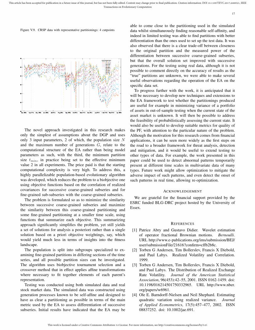
This work is licensed under a Creative Commons Attribution 3.0 License. For more information, see http://creativecommons.org/licenses/by/3.0/.
This article has been accepted for publication in a future issue of this journal, but has not been fully edited. Content may change prior to final publication. Citation information: DOI 10.1109/TEVC.2017.2688521, IEEETransactions on Evolutionary Computation
17
Figure V.9. CRSP data with representative partitionings: 4 cutpoints
The novel approach investigated in this research makesonly the simplest of assumptions about the DGP and usesonly 3 input parameters, 2 of which, the population size Nand the maximum number of generations G, relate to thecomputational structure of the EA rather than being modelparameters as such, with the third, the minimum partitionsize tmin, in practice being set to the effective minimumvalue 2 in all experiments. The price paid is that the startingcomputational complexity is very high. To address this, ahighly parallelizable population-based evolutionary algorithmwas developed, which reduces the problem to a biobjective oneusing objective functions based on the correlation of realizedcovariances for successive coarse-grained subseries and forfine-grained sub-subseries with the coarse-grained subseries.
The problem is formulated so as to minimize the similaritybetween successive coarse-grained subseries and maximizethe similarity between this coarse-grained partitioning andsome fine-grained partitioning at a smaller time scale, usingfunctions that summarize each objective. This summarizingapproach significantly simplifies the problem, yet still yieldsa set of solutions for analysis a posteriori rather than a singlesolution based on a priori objective weightings, say, whichwould yield much less in terms of insights into the fitnesslandscape.
The population is split into subgroups specialized to ex-amining fine-grained partitions in differing sections of the timeseries, and all possible partition sizes can be investigated.The algorithm uses biobjective tournament selection and acrossover method that in effect applies affine transformationswhere necessary to fit together elements of each parent’srepresentation.
Testing was conducted using both simulated data and realstock market data. The simulated data was constructed usinggeneration processes known to be self-affine and designed tohave as clear a partitioning as possible in terms of the mainmetric used by the EA to assess differentiation of successivesubseries. Initial results have indicated that the EA may be
able to come close to the partitioning used in the simulateddata whilst simultaneously finding reasonable self-affinity, andindeed in limited testing was able to find partitions with betterdifferentiation than the ones used to set up the test data. It wasalso observed that there is a clear trade-off between closenessto the original partition and the measured power of thedifferentiation between successive coarse-grained subseries,but that the overall solution set improved with successivegenerations. For the testing using real data, although it is notpossible to comment directly on the accuracy of results as the“true” partitions are unknown, we were able to make severaluseful observations regarding the operation of the EA on thespecific data set.
To progress further with the work, it is anticipated that itwill be necessary to develop new techniques and extensions tothe EA framework to test whether the partitionings producedare useful for example in minimizing variance of a portfolioof assets in out-of-sample testing when the current state of theasset market is unknown. It will then be possible to addressthe feasibility of probabilistically assessing the current state. Itwould also be useful to develop suitable metrics for quality ofthe PF, with attention to the particular nature of the problem.Although the motivation for this research comes from financialapplications, it can be seen more widely as the first steps onthe road to a broader framework for threat analysis, detectionand mitigation, and it would be useful to extend testing toother types of data. For example, the work presented in thispaper could be used to detect abnormal patterns temporarilypresent at different time scales in multivariate data of manytypes. Future work might allow optimization to mitigate theadverse impact of such patterns, and even detect the onset ofsuch patterns in real time, allowing re-optimization.
ACKNOWLEDGEMENT
We are grateful for the financial support provided by theESRC funded BLG-DRC project hosted by the University ofEssex.
REFERENCES
[1] Patrice Abry and Gustavo Didier. Wavelet estimationof operator fractional Brownian motions. Bernoulli.URL http://www.e-publications.org/ims/submission/BEJ/user/submissionFile/21616?confirm=cffb2b8c.
[2] Torben G Andersen, Tim Bollerslev, Francis X Diebold,and Paul Labys. Realized Volatility and Correlation.1999.
[3] Torben G Andersen, Tim Bollerslev, Francis X Diebold,and Paul Labys. The Distribution of Realized ExchangeRate Volatility. Journal of the American StatisticalAssociation, 96(453):42–55, 2001. ISSN 0162-1459. doi:10.1198/016214501750332965. URL http://www.nber.org/papers/w6961.
[4] Ole E. Barndorff-Nielsen and Neil Shephard. Estimatingquadratic variation using realized variance. Journalof Applied Econometrics, 17(5):457–477, 2002. ISSN08837252. doi: 10.1002/jae.691.

This work is licensed under a Creative Commons Attribution 3.0 License. For more information, see http://creativecommons.org/licenses/by/3.0/.
This article has been accepted for publication in a future issue of this journal, but has not been fully edited. Content may change prior to final publication. Citation information: DOI 10.1109/TEVC.2017.2688521, IEEETransactions on Evolutionary Computation
18
[5] Ole E Barndorff-Nielsen and Neil Shephard. Econo-metric analysis of realised covariation: high frequencycovariance, regression and correlation in financial eco-nomics. Econometrica, 72(3):885–925, 2004. ISSN1556-5068. doi: 10.2139/ssrn.305583.
[6] Jozef Barunik, Tomaso Aste, T. Di Matteo, and RuipengLiu. Understanding the source of multifractalityin financial markets. Physica A: Statistical Mech-anics and its Applications, 391(17):4234–4251, sep2012. ISSN 03784371. doi: 10.1016/j.physa.2012.03.037. URL http://linkinghub.elsevier.com/retrieve/pii/S0378437112002890.
[7] Barbara Bedowska-Sojka and Agata Kliber. Real-ized Volatility versus GARCH and Stochastic VolatilityModels. The Evidence From The WIG20 Index andthe EUR/PLN Foreign Exchange Market. PrzegladStatystyczny, 2010. URL http://keii.ue.wroc.pl/przeglad/Rok2010/Zeszyt4/2010_57_4_105-127.pdf.
[8] Fischer Black. Studies in Stock Price Volatility Changes.In Proceedings of the 1976 Business and EconomicStudies Section, pages 177–181. American StatisticalAssociation, Alexandria,Va., 1976.
[9] Tobias Blickle and Lothar Thiele. A MathematicalAnalysis of Tournament Selection. Proceedings of theSixth International Conference on Genetic Algorithms,pages 9–16, 1995. doi: 10.1.1.52.9907.
[10] Tim Bollerslev. Generalized Autoregressive ConditionalHeteroskedasticity. Journal of Econometrics, 31(3):307–327, 1986. ISSN 03044076. doi: 10.1016/0304-4076(86)90063-1.
[11] Laurent Calvet and Adlai Fisher. Forecasting multifractalvolatility. Journal of Econometrics, 105(1):27–58, 2001.ISSN 03044076. doi: 10.1016/S0304-4076(01)00069-0.
[12] Laurent E. Calvet and Adlai J. Fisher. How to ForecastLong-Run Volatility: Regime Switching and the Estim-ation of Multifractal Processes. Journal of FinancialEconometrics, 2(1):49–83, 2004. ISSN 1479-8409. doi:10.1093/jjfinec/nbh003. URL http://jfec.oupjournals.org/cgi/doi/10.1093/jjfinec/nbh003.
[13] Laurent E. Calvet and Adlai J. Fisher. MultifractalVolatility: Theory, Forecasting, and Pricing. AcademicPress, 2008. ISBN 0080559964. URL http://books.google.com/books?id=ARuiiaog0IgC&pgis=1.
[14] Laurent E. Calvet, Adlai J. Fisher, and Samuel B.Thompson. Volatility comovement: A multifrequencyapproach. Journal of Econometrics, 131(1-2):179–215,2006. ISSN 03044076. doi: 10.1016/j.jeconom.2005.01.008.
[15] Gagari Chakrabarti and Chitrakalpa Sen. Anatomy ofGlobal Stock Market Crashes. Number September 1837.Springer India, India, 2012. ISBN 978-81-322-0462-6. doi: 10.1007/978-81-322-0463-3. URL http://link.springer.com/10.1007/978-81-322-0463-3.
[16] Fei Chen, Francis X. Diebold, and Frank Schorfheide.A Markov-switching multifractal inter-trade durationmodel, with application to US equities. Journal ofEconometrics, 177(2):320–342, 2013. ISSN 03044076.doi: 10.1016/j.jeconom.2013.04.016. URL http://dx.doi.
org/10.1016/j.jeconom.2013.04.016.[17] Carlos A Coello Coello, Gary B. Lamont, and David
A. Van Veldhuizen. Evolutionary Algorithms for SolvingMulti-Objective Problems. Springer, second edition,2007. ISBN 9780387310299. URL http://books.google.com/books?id=rXIuAMw3lGAC&pgis=1.
[18] Adriana S. Cordis and Chris Kirby. Discrete stochasticautoregressive volatility. Journal of Banking and Fin-ance, 43(1):160–178, 2014. ISSN 03784266. doi:10.1016/j.jbankfin.2014.03.020.
[19] M.C. Cowgill, R.J. Harvey, and L.T. Watson. A ge-netic algorithm approach to cluster analysis. Com-puters & Mathematics with Applications, 37(7):99–108,1999. ISSN 08981221. doi: 10.1016/S0898-1221(99)00090-5. URL http://www.sciencedirect.com/science/article/pii/S0898122199000905.
[20] Anthony Davis, Alexander Marshak, Robert Cahalan, andWarren Wiscombe. The Landsat Scale Break in Stra-tocumulus as a Three-Dimensional Radiative TransferEffect: Implications for Cloud Remote Sensing. Journalof the Atmospheric Sciences, 54(2):241–260, 1997. ISSN0022-4928. doi: 10.1175/1520-0469(1997)054<0241:TLSBIS>2.0.CO;2.
[21] Kalyanmoy Deb and Amrit Pratap. A fast and elit-ist multiobjective genetic algorithm: NSGA-II. IEEETransactions on Evolutionary Computation, 6(2):182–197, 2002. URL http://ieeexplore.ieee.org/xpls/abs_all.jsp?arnumber=996017.
[22] Gustavo Didier and Vladas Pipiras. Integral represent-ations and properties of operator fractional Brownianmotions. Bernoulli, 17(1):1–33, 2011. ISSN 1350-7265.doi: 10.3150/10-BEJ259. URL http://projecteuclid.org/euclid.bj/1297173831.
[23] Ralph Nelson Elliott. Nature’s Law. Snowball Publish-ing, 2010.
[24] Ralph Nelson Elliott. The Wave Principle. SnowballPublishing, 2012.
[25] Robert F Engle. Autoregressive Conditional Heteroske-dasticity with Estimates of the Variance of UK Inflation.Econometrica: Journal of the Econometric Society, 50(4):987–1007, 1982.
[26] Eugene F. Fama. Mandelbrot and the Stable ParetianHypothesis. The Journal of Business, 36(4):420–429,1963. ISSN 00219398; 15375374. URL http://www.jstor.org/stable/2350971.
[27] P J Flynn, A K Jain, M N Murty, P J Flynn, AzrielRosenfeld, K Bowyer, N Ahuja, and A K Jain. DataClustering: A Review. 2000. ISSN 03600300. doi: 10.1145/331499.331504.
[28] Rene Garcia and Pierre Perron. An analysis of thereal interest rate under regime shifts. The Review ofEconomics and Statistics, 78(1):111–125, 1996. URLhttp://www.jstor.org/stable/2109851.
[29] Weiyu Guo and Mark E. Wohar. Identifying RegimeChanges in Market Volatility. Journal of FinancialResearch, 29(1):79–93, mar 2006. ISSN 0270-2592.doi: 10.1111/j.1475-6803.2006.00167.x. URL http://doi.wiley.com/10.1111/j.1475-6803.2006.00167.x.

This work is licensed under a Creative Commons Attribution 3.0 License. For more information, see http://creativecommons.org/licenses/by/3.0/.
This article has been accepted for publication in a future issue of this journal, but has not been fully edited. Content may change prior to final publication. Citation information: DOI 10.1109/TEVC.2017.2688521, IEEETransactions on Evolutionary Computation
19
[30] Donatien Hainaut. A fractal version of the Hull-Whiteinterest rate model. Economic Modelling, 31(1989):1–15,2010. ISSN 02649993. doi: 10.1016/j.econmod.2012.11.041. URL http://dx.doi.org/10.1016/j.econmod.2012.11.041.
[31] James D. Hamilton. Rational-Expectations EconometricAnalysis of Changes in Regime. Journal of EconomicDynamics and Control, 12(2/3):385–423, 1988. ISSN0165-1889.
[32] JD Hamilton. A new approach to the economic analysisof nonstationary time series and the business cycle.Econometrica: Journal of the Econometric Society, 57(2):357–384, 1989. URL http://www.jstor.org/stable/1912559.
[33] JD Hamilton. Analysis of time series subject tochanges in regime. Journal of Econometrics, 45:39–70,1990. URL http://www.sciencedirect.com/science/article/pii/0304407690900939.
[34] Julia Handl and Joshua Knowles. An evolutionaryapproach to multiobjective clustering. IEEE Transactionson Evolutionary Computation, 11(1):56–76, 2007. ISSN1089778X. doi: 10.1109/TEVC.2006.877146.
[35] Harold Edwin Hurst. Long-term storage capacity ofreservoirs. Transactions of the American Society of CivilEngineers, 116:770–808, 1951.
[36] Julien Idier. (Re)correlation: a Markov switch-ing multifractal model with time varying correlations.2009. URL https://papers.ssrn.com/sol3/papers.cfm?abstract_id=1580075.
[37] Julien Idier. short-term comovements in stock markets:the use of Markov-switching multifractal models. TheEuropean Journal of Finance, 17(1):27–48, 2011. ISSN1351-847X. doi: 10.1080/13518470903448440.
[38] Carla Inclan and GC Tiao. Use of cumulative sumsof squares for retrospective detection of changes ofvariance. Journal of the American Statistical Association,89(427):913–923, 1994. URL http://www.tandfonline.com/doi/abs/10.1080/01621459.1994.10476824.
[39] E. Keogh, S. Chu, D. Hart, and M. Pazzani. Anonline algorithm for segmenting time series. Proceedings2001 IEEE International Conference on Data Mining,pages 289–296, 2001. ISSN 15504786. doi: 10.1109/ICDM.2001.989531. URL http://ieeexplore.ieee.org/lpdocs/epic03/wrapper.htm?arnumber=989531.
[40] M. Laumanns, L. Thiele, and E. Zitzler. Runningtime analysis of multiobjective evolutionary algorithmson pseudo-Boolean functions. IEEE Transactions onEvolutionary Computation, 8(2):170–182, 2004. ISSN1089-778X. doi: 10.1109/TEVC.2004.823470.
[41] T. Warren Liao. Clustering of time series data - a survey.Pattern Recognition, 38(11):1857–1874, 2005.
[42] Ruipeng Liu. Multivariate Multifractal Models : Estima-tion of Parameters and Applications to Risk Management.PhD thesis, 2008.
[43] Ruipeng Liu and Thomas Lux. Higher Dimensional Mul-tifractal Processes : A GMM Approach. In ICCEF 2010book of abstracts. Society for Computational Economics,2012.
[44] Ruipeng Liu and Thomas Lux. Non-homogeneousvolatility correlations in the bivariate multifractal model.The European Journal of Finance, (May 2015):1–21,2014. ISSN 1351-847X. doi: 10.1080/1351847X.2014.897960. URL http://www.tandfonline.com/doi/abs/10.1080/1351847X.2014.897960.
[45] Thomas Lux. The Markov-switching multifractal modelof asset returns: GMM estimation and linear forecastingof volatility. Journal of business & economic statistics,26(2):194–210, 2008. ISSN 07350015. doi: 10.1198/073500107000000403. URL http://wrap.warwick.ac.uk/1749/.
[46] Thomas Lux. Flexible and Robust Modelling of Volat-ility Comovements : A Comparison of Two MultifractalModels. 2010.
[47] Thomas Lux and Taisei Kaizoji. Forecasting volatilityand volume in the Tokyo Stock Market: Long memory,fractality and regime switching. Journal of EconomicDynamics and Control, 31(6):1808–1843, 2007. ISSN01651889. doi: 10.1016/j.jedc.2007.01.010.
[48] B Mandelbrot. How long is the coast of Britain?Statistical self-similarity and fractional dimension. Sci-ence, 156(3775):636–638, 1967. ISSN 0036-8075. doi:10.1126/science.156.3775.636.
[49] Benoit Mandelbrot. The Variation of Certain SpeculativePrices. The Journal of Business, 36(4):394–419, 1963.ISSN 00219398; 15375374. URL http://link.springer.com/chapter/10.1007/978-1-4757-2763-0_14.
[50] Benoit Mandelbrot. The variation of some other specu-lative prices. Journal of Business, 40(4):393–413, 1967.URL http://www.jstor.org/stable/2351623.
[51] Benoit Mandelbrot, Adlai Fisher, and Laurent Calvet. AMultifractal Model of Asset Returns. 1997. URL http://search.ebscohost.com/login.aspx?direct=true&db=bth&AN=8752064&site=bsi-live&scope=site.
[52] Benoit B. Mandelbrot and John W. Van Ness. FractionalBrownian Motions, Fractional Noises and Applications.SIAM Review, 10(4):422–437, 1968. ISSN 0036-1445.doi: 10.1137/1010093.
[53] RN Mantegna. Hierarchical structure in financial mar-kets. The European Physical Journal B, 11:193–197, 1999. URL http://link.springer.com/article/10.1007/s100510050929.
[54] Ujjwal Maulik and Sanghamitra Bandyopadhyay. Ge-netic algorithm-based clustering technique. Pattern Re-cognition, 33:1455–1465, 2000. ISSN 00313203. doi:10.1016/S0031-3203(99)00137-5.
[55] Angelo Melino and Stuart M. Turnbull. PricingForeign Currency Options with Stochastic Volatil-ity. Journal of Econometrics. Jul/Aug90, 45(1/2):239–265. 27p. 7 Charts, 1990. ISSN 0304-4076. URL http://www.sciencedirect.com/science/article/pii/0304407690901008.
[56] Lars Black Mogensen. Models of Changing Volatility :A Multifractal Approach. PhD thesis, Aarchus School ofBusiness, 2011.
[57] Raffaello Morales, T Di Matteo, and Tomaso Aste.Dependency structure and scaling properties of financial

This work is licensed under a Creative Commons Attribution 3.0 License. For more information, see http://creativecommons.org/licenses/by/3.0/.
This article has been accepted for publication in a future issue of this journal, but has not been fully edited. Content may change prior to final publication. Citation information: DOI 10.1109/TEVC.2017.2688521, IEEETransactions on Evolutionary Computation
20
time series are related. Scientific reports, 4:4589,jan 2014. ISSN 2045-2322. doi: 10.1038/srep04589.URL http://www.pubmedcentral.nih.gov/articlerender.fcgi?artid=3980463&tool=pmcentrez&rendertype=abstract.
[58] Noemi Nava, T Di Matteo, and Tomaso Aste. Anomalousvolatility scaling in high frequency financial data. 2015.
[59] Jon D. Pelletier and Donald L. Turcotte. Self-affinetime series: II. Applications and models. In Advancesin Geophysics Vol. 40, pages 91–166. Academic Press,1997. URL http://arxiv.org/abs/physics/9705038.
[60] Lewis Fry Richardson. The problem of contiguity :An appendix to statistics of deadly quarrels. Generalsystems: Yearbook of the Society for the Advancement ofGeneral Systems Theory, 6:139–187, 1961.
[61] Peter J. Rousseeuw. Silhouettes: A graphical aid to theinterpretation and validation of cluster analysis. Journalof Computational and Applied Mathematics, 20:53–65,nov 1987. ISSN 03770427. doi: 10.1016/0377-0427(87)90125-7. URL http://linkinghub.elsevier.com/retrieve/pii/0377042787901257.
[62] Martin Rypdal and Ola Løvsletten. Multifractal modelingof short-term interest rates. 2011. URL http://arxiv.org/abs/1111.5265.
[63] A Sansó, V Aragó, and JL Carrion. Testing forchanges in the unconditional variance of financial timeseries. Revista de Economía Financiera, 4:32–53,2004. URL http://www.aefin.es/AEFIN_data/articulos/pdf/A4-2_443809.pdf.
[64] Won Min Song, T. Di Matteo, and Tomaso Aste. Hier-archical information clustering by means of topologicallyembedded graphs. PLoS ONE, 7(3):1–14, 2012. ISSN19326203. doi: 10.1371/journal.pone.0031929.
[65] N Srinivas and K Deb. Muiltiobjective optimization usingnondominated sorting in genetic algorithms. Evolution-ary Computation, 2(3):221–248, 1994. URL http://www.mitpressjournals.org/doi/abs/10.1162/evco.1994.2.3.221.
[66] Michele Tumminello, Fabrizio Lillo, and RN Mantegna.Correlation, hierarchies, and networks in financial mar-kets. Journal of Economic Behavior & Organization,75(1):40–58, 2010. URL http://www.sciencedirect.com/science/article/pii/S0167268110000077.
[67] Victor Venema. p-model multifractal time series, 2006.URL http://www2.meteo.uni-bonn.de/staff/venema/themes/surrogates/pmodel/.
[68] Darrell Whitley, Soraya Rana, and Robert BHeckendorn. The island model genetic algorithm:On separability, population size and convergence.Journal of Computing and Information Technology,7:33–47, 1999. doi: 10.1.1.36.7225. URLhttp://citeseerx.ist.psu.edu/viewdoc/download?doi=10.1.1.36.7225&rep=rep1&type=pdf.
[69] Qingfu Zhang and Hui Li. MOEA/D: A multiobjectiveevolutionary algorithm based on decomposition. IEEETransactions on Evolutionary Computation, 11(6):712–731, 2007. URL http://ieeexplore.ieee.org/xpls/abs_all.jsp?arnumber=4358754.
[70] Jian Zhong and Xin Zhao. Modeling Complicated
Behavior of Stock Prices Using Discrete Self-ExcitedMultifractal Process. Systems Engineering Procedia, 3(2011):110–118, 2012. ISSN 22113819. doi: 10.1016/j.sepro.2011.11.015.
Christopher M. Taylor (M’16) received theM.Sc. degree in financial economics from the University ofOxford, U.K. in 2006 and the M.Sc. degree in operationalresearch from the University of Essex, U.K. in 2014. He iscurrently pursuing the Ph.D. degree in operational researchfrom the University of Essex.
He has over 20 years’ experience working as a financeprofessional in fund management and investment banking inAsia, U.K. and U.S.A.
Abdellah Salhi is Professor of Opera-tional Research at the University of Essex, U.K.with interestsin the design, analysis and application of optimisation al-gorithms and heuristics. He was educated to degree level atthe University of Constantine, in Algeria. He obtained hisPhD from Aston University in Birmingham, UK. He acted asResearch Fellow on a number of projects in OR and HPCat the universities of Leeds, Edinburgh and Southampton.He recently led projects such as Workforce Scheduling inContainer Ports, the Beeswax project on Optimum Placementof Beehives for Optimum Pollination, and the Smart TownCentre. He has published over 70 articles in journals suchas Annals of OR, Information Processing Letters and AppliedSoft Computing. He has recently introduced the Plant Propaga-tion Algorithm for global optimisation, a heuristic inspired bythe way strawberry plants propagate.