chiroptical spectroscopic studies on surfactants, other...

Chiroptical Spectroscopic Studies on Surfactants, Other Aggregating Systems, and Natural Products

By

Cody Lance Covington

Dissertation

Submitted to the Faculty of the

Graduate School of Vanderbilt University

in partial fulfillment of the requirements

for the degree of

DOCTOR OF PHILOSOPHY

in

Chemistry

May, 2016

Nashville, Tennessee

Approved:

Prasad L. Polavarapu, Ph.D. Timothy P. Hanusa, Ph.D.

Terry P. Lybrand, Ph.D. Janet E. Macdonald, Ph.D.

Kalman Varga, Ph.D.

ii

To Charlsey and Connor

iii

Acknowledgment

Firstly, I would like to express my sincere gratitude to my advisor Prof. Prasad Polavarapu for his

support throughout my project. He was always willing to help with whatever problems I could stumble

into. His guidance helped me in research and in writing of this document. I am very grateful for his

concern for my future employment after I graduate, and I look forward to future collaborations.

Many thanks to Prof. Timothy Hanusa, in who’s lab I did a rotation my first year and learned many

things about calculations and synthesis. I would like to thank Prof. Terry Lybrand for helping with

numerous aspects of the molecular dynamics simulations. Whom, I can always count on insightful

discussions and good questions. Thanks to Prof. Janet Macdonald for being on my committee.

Surfactants and nanoparticles are similar in many ways, and I greatly appreciate her expertise. Many

thanks to Prof. Kalman Varga from the Physics department for being a member of my committee, his

expertise in DFT and fragmentation of small molecules was greatly appreciated for my independent

research proposal.

I would like to send a shout out to Prof. Joel Tellinghuisen who really trained me to think like a

physical chemist and always has a good fish story. I would also like to thank others who have helped me:

Raghavan Vijay, Fernando Martins, Brett Covington, Jason Gerding, Francesca Gruppi, Jonathan Sheehan

and Jarrod Smith.

I thank NSF (CHE-0804301 and CHE-1464874) for financial support. This work was conducted in

part using the resources of the Advanced Computing Center for Research and Education (ACCRE) at

Vanderbilt University, Nashville, TN.

Last, but certainly not least, I thank my wife Charlsey for understanding my many years of long

hours and distracted thoughts.

iv

Table of Contents

Acknowledgment ......................................................................................................................................... iii

List of Tables ................................................................................................................................................ vi

List of Figures .............................................................................................................................................. vii

List of Abbreviations/Nomenclature/Symbols............................................................................................ xii

Chapter 1 Introduction ................................................................................................................................. 1

Optical Rotatory Dispersion (ORD) ............................................................................................. 1

Electronic Circular Dichroism (ECD) ............................................................................................ 2

Vibrational Circular Dichroism (VCD) .......................................................................................... 3

Quantum Chemistry (QC) ........................................................................................................... 4

Molecular Dynamics (MD) .......................................................................................................... 4

Similarity Methods ...................................................................................................................... 5

Project perspective ..................................................................................................................... 6

Chapter 2 The ORD of aggregating systems much simpler than surfactants ............................................... 7

Introduction ................................................................................................................................ 7

Derivation of SOR for a Homochiral monomer-dimer mixture .................................................. 8

Wavelength resolved SOR of Pantolactone in monomeric and dimeric form ........................... 9

Calculated SOR for the pantolactone monomer and dimer ..................................................... 10

Enantiomeric Mixtures and the Horeau Effect ......................................................................... 11

Derivation of SOR for a Heterochiral monomer-dimer mixture ............................................... 13

The case of pantolactone ......................................................................................................... 15

The case of 2-hydroxy-3-pinanone ........................................................................................... 15

Calculated SOR for (1S,2S,5S)-(−)-2-hydroxy-3-pinanone ........................................................ 17

The case of 2-methyl-2-ethyl-succinic acid .............................................................................. 19

Conclusion ................................................................................................................................ 21

Chapter 3 The Chiroptical Properties of Surfactants .................................................................................. 22

Introduction .............................................................................................................................. 22

Computational Modeling of Surfactant Systems ...................................................................... 28

Results and analysis .................................................................................................................. 29

Conclusions for LEP calculations ............................................................................................... 42

Details on the MD simulations ................................................................................................. 43

Experimental Methods ............................................................................................................. 45

Chapter 4 The Dissymmetry Factor spectrum: A novel chiroptical spectral analysis method ................... 46

Introduction .............................................................................................................................. 46

Method ..................................................................................................................................... 47

Results ....................................................................................................................................... 48

Conclusions ............................................................................................................................... 66

Experimental ............................................................................................................................. 66

Chapter 5 The AC of Centratherin ............................................................................................................... 68

Introduction .............................................................................................................................. 68

Results ....................................................................................................................................... 69

v

Conclusion ................................................................................................................................ 73

Experimental ............................................................................................................................. 73

Chapter 6 The AC of (+)-3-ishwarone ......................................................................................................... 75

Introduction .............................................................................................................................. 75

Results and Discussion .............................................................................................................. 76

Conclusion ................................................................................................................................ 82

Experimental ............................................................................................................................. 82

Chapter 7 The AC of (‒)-Hypogeamicin B ................................................................................................... 83

Introduction .............................................................................................................................. 83

Result and Discussion ............................................................................................................... 84

Conclusion ................................................................................................................................ 90

Experimental ............................................................................................................................. 90

Chapter 8 The AC of (‒)-Agathisflavone...................................................................................................... 91

Introduction .............................................................................................................................. 91

Results ....................................................................................................................................... 92

Conclusions ............................................................................................................................. 100

Experimental ........................................................................................................................... 100

Chapter 9 Analysis of the Exciton Chirality (EC) Method for VCD ............................................................ 102

Introduction ............................................................................................................................ 102

The Exciton Chirality (EC) Method .......................................................................................... 103

Results ..................................................................................................................................... 108

Conclusions ............................................................................................................................. 111

Chapter 10 Conclusions ............................................................................................................................ 112

Appendix A Concepts used in the analysis of surfactant and aggregate systems ............................ 114

Appendix B Additional Experimental Data ....................................................................................... 117

References ................................................................................................................................................ 121

vi

List of Tables

Table 2-1: Measured SOR values for (R)-(−)-pantolactone in CCl4 .............................................................. 10

Table 2-2: Fitted SOR values of the (R)-(−)-pantolactone monomer and dimer in CCl4 ............................. 10

Table 3-1: Boltzmann weights from Cam-B3LYP/Aug-cc-pVDZ/PCM calculations with and without an

applied electric field ....................................................................................................................... 37

Table 3-2: Dihedral occupancies of 40 LEP Micelle with PM6 forces ......................................................... 40

Table 3-3: Dihedral occupancies of 1 LEP in water with PM6 forces .......................................................... 40

Table 3-4: LEP simulation details ................................................................................................................ 45

Table 4-1: Details for the six VDF test compounds. *Calculated for the study118-121 .................................. 49

Table 4-2: Maximum similarity ratings for the six VDF test cases .............................................................. 52

Table 7-1: Maximum similarity ratings from all solvation models for (‒)-hypogeamicin B in DMSO ........ 90

Table 9-1: Conformer populations for SpA and SpB using electronic energies and Gibbs energies ........ 106

Table 9-2: Quantum and NDEC results for SpA for all conformers ........................................................... 109

Table 9-3: Quantum and NDEC results for SpB for all conformers ........................................................... 110

Table 10-1: Computer time required for various calculations run on 2.3-3.0 GHz Intel Xeon Westmere

dual quad or dual hex processsors using Gaussian 09................................................................. 113

vii

List of Figures

Figure 2-1: Pantolactone with equilibrium between monomer and dimer ................................................. 9

Figure 2-2: (left) The calculated SORs of the pantolactone monomer and (right) dimer compared to

experiment in CCl4 ......................................................................................................................... 11

Figure 2-3: The Horeau effect in 2-methyl-2-ethyl succinic acid, shown op vs ee67 ................................... 12

Figure 2-4: Compounds that exhibit the Horeau effect67-70 ........................................................................ 12

Figure 2-5: Some examples of the exact solution of the monomer-dimer Horeau equations ................... 14

Figure 2-6: Measured Horeau curves for pantolactone ............................................................................. 15

Figure 2-7: (left) Horeau effect previously reported69 in CHCl3 and (right) performed in our lab in CCl4 .. 16

Figure 2-8: The concentration dependence of (1S,2S,5S)-(−)-2-hydroxy-3-pinanone in CCl4 .................... 16

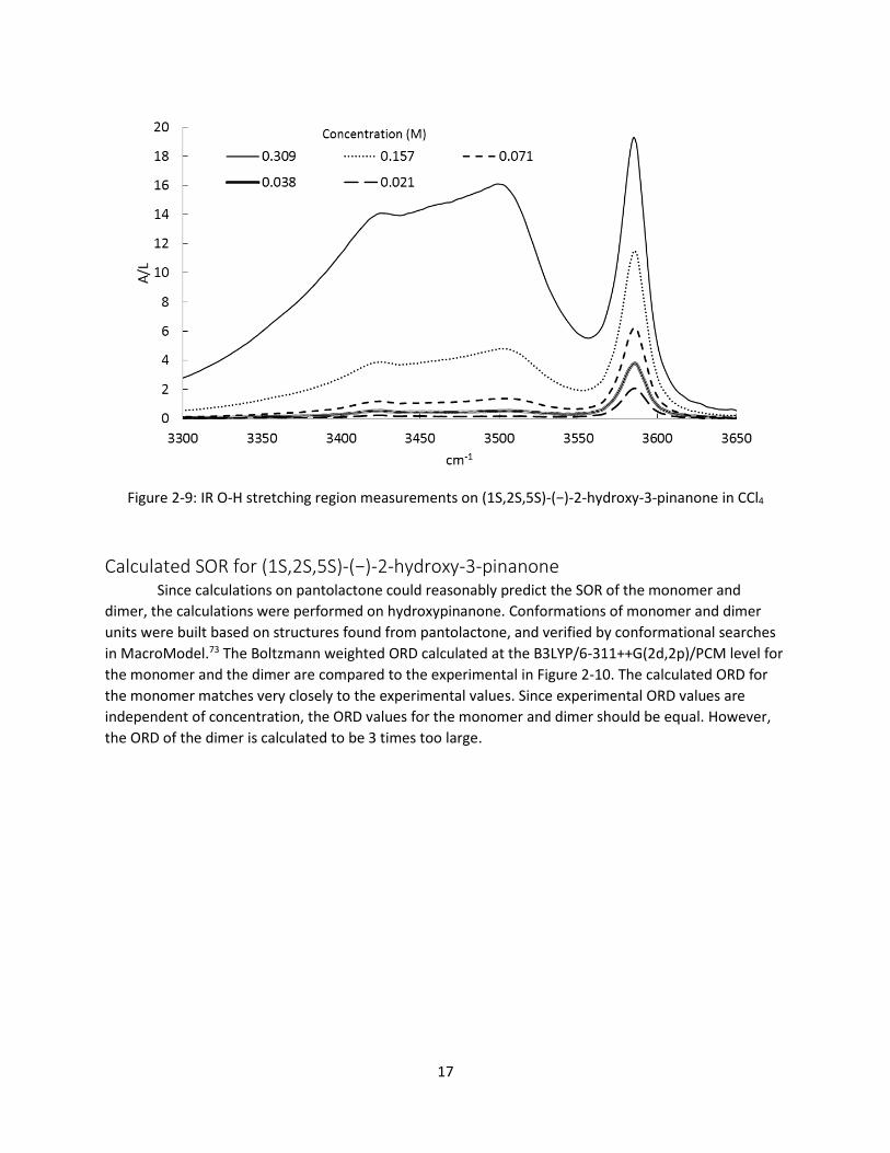
Figure 2-9: IR O-H stretching region measurements on (1S,2S,5S)-(−)-2-hydroxy-3-pinanone in CCl4 ...... 17

Figure 2-10: The calculated ORD for (1S,2S,5S)-(−)-2-hydroxy-3-pinanone at the B3LYP/6-

311++G(2d,2p)/PCM level compared to experiment in CCl4 ......................................................... 18

Figure 2-11: The experimental VCD for both the monomer and dimer of (1S,2S,5S)-(−)-2-hydroxy-3-

pinanone in CCl4, arrows showing the bands most effected by aggregation ................................ 19

Figure 2-12: The VCD for both the monomer and dimer of (1S,2S,5S)-(−)-2-hydroxy-3-pinanone

calculated at the B3LYP/6-311++G(2d,2p) level ............................................................................ 19

Figure 2-13: An optimized monomer unit of (S)-2-methyl-2-ethyl-succinic acid ....................................... 20

Figure 2-14: An optimized homochiral tetramer unit of (S)-2-methyl-2-ethyl-succinic acid...................... 20

Figure 3-1: Some structures of aggregating surfactants ............................................................................. 22

Figure 3-2: Structures of some key surfactants in this work ...................................................................... 23

Figure 3-3: SOR and surface tension as a function of concentration for FLNa in water and methanol ..... 23

Figure 3-4: SOR as a function of concentration for TAR12 in water, data from Raghavan Vijay

(unpublished) ................................................................................................................................. 24

Figure 3-5: SOR of LEP and the aggregation number79 ............................................................................... 24

Figure 3-6: SOR of LET changing with aggregation number and temperature79 ........................................ 25

Figure 3-7: ORD measurements on L-LEP in water ..................................................................................... 26

Figure 3-8: SOR for L-LEP as a function of concentration, linear and log scale .......................................... 26

Figure 3-9: ECD measurements on LEP in water ......................................................................................... 27

Figure 3-10: Observed ORD compared to KK-Transformed ECD ................................................................ 27

Figure 3-11: SOR calculations on aqueous EEP system at various levels of theory, 625 snapshots for all

except the B3LYP/Aug-cc-pVDZ calculations which used 274 snapshots ...................................... 28

Figure 3-12: (left) Average ORD and (right) Average ORD excluding resonant snapshots for EEP ............ 29

Figure 3-13: Trends in calculated SOR on LEP clusters, using B3LYP/6-31G* ............................................. 30

Figure 3-14: TEM images of LEP (left) 50 mM and (right) 200 mM79 .......................................................... 30

Figure 3-15: SOR of 200mM LEP as a function of ee at 25°C ...................................................................... 31

Figure 3-16: The dihedral angles φ and ψ (bold indicating the atoms that define them), Carbonyl

chromophore also shown .............................................................................................................. 32

Figure 3-17: Histograms of the φ and ψ values in 1 and 40 LEP MD simulations ...................................... 32

Figure 3-18: LEP with Z and Y axes identified ............................................................................................. 33

Figure 3-19: Electric field along Z-Axis (top) with and (bottom) without water ......................................... 34

viii

Figure 3-20: Electric field along x and y Axes with water from 200 LEP bilayer simulation for specific

conformations (φ and ψ values) .................................................................................................... 35

Figure 3-21: ORD calculations on EEP with external field applied along the Z-axis. Boltzmann weighted

using all the same electronic energies (left), and Boltzmann weighted using the electronic

energies in the external field (right) .............................................................................................. 36

Figure 3-22: ORD curves comparing calculations on EEP with and without external fields with

experimental EEP and LEP(200 mM) values taken in water .......................................................... 36

Figure 3-23: An Example QM region containing 1 LEP headgroup and 25 explicit water molecules ......... 38

Figure 3-24: QM/MM-MD simulations with charges included over (left) infinite and (right) a limited

range .............................................................................................................................................. 38

Figure 3-25: Dihedral angle ψ populations from QM/MM-MD with PM6 Hamiltonian ............................ 39

Figure 3-26: Dihedral angle φ populations from QM/MM-MD with PM6 Hamiltonian ............................. 39

Figure 3-27: ORD calculated from QM/MM-MD conformational populations .......................................... 41

Figure 3-28: ECD calculated using populations found from QM/MM-MD at the....................................... 41

Figure 3-29: Radial distribution functions comparing EEP buffered solvent exchange .............................. 44

Figure 4-1: Initial compounds considered in the VDF study ....................................................................... 49

Figure 4-2: The calculated and experimental VA spectra of (3R)-(+)-methylcyclopentanone ................... 50

Figure 4-3: The calculated and experimental VCD spectra of (3R)-(+)-methylcyclopentanone ................. 50

Figure 4-4: The calculated and experimental VDF spectra of (3R)-(+)-methylcyclopentanone. τA was taken

to be 2.4 L mol-1 cm-1 ..................................................................................................................... 51

Figure 4-5: Vibrational similarity analysis of (3R)-(+)-methylcyclopentanone ........................................... 51

Figure 4-6: (aR)-(+)-3,3'-diphenyl-[2,2'-binaphthalene]-1,1'-diol, also called Vanol .................................. 53

Figure 4-7: The EA of (aR)-(+)-Vanol in acetonitrile .................................................................................... 53

Figure 4-8: The ECD of (aR)-(+)-Vanol in acetonitrile .................................................................................. 53

Figure 4-9: The EDF of (aR)-(+)-Vanol in acetonitrile .................................................................................. 54

Figure 4-10: Electronic similarity analysis of (aR)-(+)-Vanol in acetonitrile ................................................ 54

Figure 4-11: Raman spectrum of (1S)-(-)-α-pinene as neat liquid .............................................................. 55

Figure 4-12: The ROA spectrum of (1S)-(-)-α-pinene as neat liquid ........................................................... 56

Figure 4-13: The CID spectrum of (1S)-(-)-α-pinene as neat liquid ............................................................. 56

Figure 4-14: The Raman similarity analysis of (1S)-(-)-α-pinene as neat liquid .......................................... 57

Figure 4-15: Bultinck’s confidence level data with the confidence at various points shown53 .................. 58

Figure 4-16: The structures of BN and DBBN .............................................................................................. 58

Figure 4-17: The EA of (‒)-(aS)-BN in multiple solvents .............................................................................. 59

Figure 4-18: The ECD of (‒)-(aS)-BN in multiple solvents ........................................................................... 59

Figure 4-19: The EDF of (‒)-(aS)-BN in multiple solvents ............................................................................ 60

Figure 4-20: The calculated EDF of (‒)-(aS)-BN in the gas phase and with acetonitrile complexes and PCM

CAM-B3LYP/Aug-cc-pVDZ, wg=10 nm ............................................................................................ 61

Figure 4-21: The EA of (+)-(aS)-DBBN in multiple solvents ......................................................................... 62

Figure 4-22: The ECD of (+)-(aS)-DBBN in multiple solvents ....................................................................... 62

Figure 4-23: The EDF of (+)-(aS)-DBBN in multiple solvents ....................................................................... 63

Figure 4-24: The calculated EDF of (+)-(aS)-DBBN in the gas phase and with acetonitrile complexes and

PCM, CAM-B3LYP/6-311++G(2d,2p), wg=10 nm ............................................................................ 64

Figure 4-25: The structure of CSA2, a chiral sulfonic acid studied in collaboration with Professor Daniel

Armstrong, University of Texas at Arlington .................................................................................. 64

ix

Figure 4-26: The VA spectra of CSA2 in methanol and DMSO .................................................................... 65

Figure 4-27: The VCD spectra of CSA2 in methanol and DMSO.................................................................. 65

Figure 4-28: The VDF spectra of CSA2 in methanol and DMSO .................................................................. 66

Figure 5-1: Centratherin .............................................................................................................................. 68

Figure 5-2: The EA of (-)-(6R,7R,8S,10R,3'Z)-centratherin experimental in acetonitrile and calculated at

the CAM-B3LYP/Aug-cc-pVDZ/PCM level ...................................................................................... 69

Figure 5-3: The ECD of (-)-(6R,7R,8S,10R,3'Z)-centratherin experimental in acetonitrile and calculated at


Figure 5-4: The EDF of (-)-(6R,7R,8S,10R,3'Z)-centratherin experimental in acetonitrile and calculated at


Figure 5-5: Electronic spectra similarity plot of (-)-(6R,7R,8S,10R,3'Z)-centratherin experimental in

acetonitrile compared to CAM-B3LYP/Aug-cc-pVDZ/PCM calculations ........................................ 70

Figure 5-6: The ORD of (-)-(6R,7R,8S,10R,3'Z)-centratherin experimental in acetonitrile and calculated at


Figure 5-7: The VA spectrum of (-)-(6R,7R,8S,10R,3'Z)-centratherin experimental in acetonitrile and

calculated at the B3LYP/Aug-cc-pVDZ/PCM level .......................................................................... 71

Figure 5-8: The VCD spectrum of (-)-(6R,7R,8S,10R,3'Z)-centratherin experimental in acetonitrile and


Figure 5-9: The VDF spectrum of (-)-(6R,7R,8S,10R,3'Z)-centratherin experimental in acetonitrile and


Figure 5-10: Vibrational similarity plot of (-)-(6R,7R,8S,10R,3'Z)-centratherin experimental in acetonitrile

compared to B3LYP/Aug-cc-pVDZ/PCM calculations .................................................................... 73

Figure 6-1: 3-Ishiwarone ............................................................................................................................. 76

Figure 6-2: Comparison of experimental EA spectrum of (+)-3-ishwarone in acetonitrile (scaled by 0.16)

with those predicted for four diastereomers calculated at the B3LYP/Aug-cc-pVDZ/PCM level .. 77

Figure 6-3: Comparison of experimental ECD spectrum of (+)-3-ishwarone in acetonitrile (scaled by 0.16)


Figure 6-4: Comparison of experimental EDF spectrum of (+)-3-ishwarone in acetonitrile with those

predicted for four diastereomers calculated at the B3LYP/Aug-cc-pVDZ/PCM level .................... 78

Figure 6-5: Comparison of experimental ORD spectrum of (+)-3-ishwarone in chloroform with those


Figure 6-6: Comparison of experimental VA spectrum of (+)-3-ishwarone in chloroform with those


Figure 6-7: Comparison of experimental VCD spectrum of (+)-3-ishwarone in chloroform (scaled by 0.5)


Figure 6-8: Comparison of experimental VDF spectrum of (+)-3-ishwarone in chloroform (scaled by 0.5)


Figure 6-9: Similarity plots for (+)-3-ishwarone in chloroform compared to the four possible

diastereomers calculated at the B3LYP/Aug-cc-pVDZ/PCM level ................................................. 81

Figure 7-1: Hypogeamicins A−D .................................................................................................................. 83

Figure 7-2: The 4 possible stereoisomers of Hypogeamicin B labeled 1-4 ................................................. 84

Figure 7-3: The EA spectra for (‒)-hypogeamicin B in acetonitrile with those predicted for the four


x

Figure 7-4: The ECD spectra for (‒)-hypogeamicin B in acetonitrile with those predicted for the four


Figure 7-5: The EDF spectra for (‒)-hypogeamicin B in acetonitrile with those predicted for the four


Figure 7-6: Electronic CD similarity analysis (‒)-hypogeamicin B in acetonitrile with those predicted for

the four diastereomers calculated at the B3LYP/Aug-cc-pVDZ/PCM level ................................... 86

Figure 7-7: The solvation models chosen to represent hypogeamicin B .................................................... 87

Figure 7-8: VCD spectra for (‒)-hypogeamicin B in DMSO compared to DMSO/Closed solvation model . 88

Figure 7-9: VA spectra for (‒)-hypogeamicin B in DMSO compared to DMSO/Closed solvation model .... 88

Figure 7-10: VDF spectra for (‒)-hypogeamicin B in DMSO compared to DMSO/Closed solvation model 89

Figure 7-11: Vibrational similarity plots for (‒)-hypogeamicin B in DMSO compared to DMSO/Closed

solvation model ............................................................................................................................. 89

Figure 8-1: Flavone backbone and Agathisflavone ..................................................................................... 91

Figure 8-2: The calculated and experimental EA spectra of (‒)-agathisflavone. ........................................ 92

Figure 8-3: The experimental ECD spectrum of (‒)-agathisflavone compared to the calculated spectrum

with the (aS) AC at the CAM-B3LYP/6-311++G(2d,2p)/PCM level ................................................. 93

Figure 8-4: The experimental EDF spectrum of (‒)-agathisflavone compared to the calculated spectrum


Figure 8-5: The electronic spectral similarity plot of (‒)-agathisflavone compared to the calculated

spectrum with the (aS) AC at the CAM-B3LYP/6-311++G(2d,2p)/PCM level ................................ 94

Figure 8-6: The ORD of (‒)-agathisflavone compared to the calculated spectrum with the (aS) AC at the

CAM-B3LYP/6-311++G(2d,2p)/PCM level ...................................................................................... 94

Figure 8-7: The experimental VA spectrum of (‒)-agathisflavone compared to the calculated spectrum at

the B3LYP/6-311++G(2d,2p)/PCM level ......................................................................................... 95

Figure 8-8: The experimental VCD spectrum of (‒)-agathisflavone compared to the calculated spectrum


Figure 8-9: The experimental VDF spectrum of (‒)-agathisflavone compared the calculated spectrum


Figure 8-10: The vibrational similarity plot comparing (‒)-agathisflavone to the (aS) AC at the ............... 97

Figure 8-11: A snapshot from the agathisflavone-methanol MD simulation. All methanol molecules

within 2.5 Å of a hydrogen bonding group are shown .................................................................. 97

Figure 8-12: The experimental VCD spectrum of (‒)-agathisflavone compared to the calculated spectra

with the (aS) AC from MD trajectories at the B3LYP/6-31G*/PCM level ...................................... 98

Figure 8-13: The experimental VA spectrum of (‒)-agathisflavone compared to the calculated spectra

from MD trajectories at the B3LYP/6-31G*/PCM level ................................................................. 98

Figure 8-14: The experimental VDF spectrum of (‒)-agathisflavone compared to the calculated spectra

with the (aS) AC from MD trajectories at the B3LYP/6-31G*/PCM level ...................................... 99

Figure 8-15: The vibrational similarity plot comparing (‒)-agathisflavone to the (aS) AC from closed-OH

MD trajectory at the B3LYP/6-31G*/PCM level, comparing 1500-1200 cm-1 ............................... 99

Figure 9-1: The structure of (2’R,6S,7S)-spiroindicumide A diacetate and (2’R,6S,7R)-spiroindicumide B

diacetate, labeled SpA and SpB, and identifying the four carbonyl groups as A-D. .................... 103

Figure 9-2: The VA spectrum of SpA in CHCl3 with the calculated spectrum at the B3LYP/TZVP/PCM level

..................................................................................................................................................... 107

Figure 9-3: The VCD spectrum of SpA with the calculated spectrum at the B3LYP/TZVP/PCM level ...... 107

xi

Figure 9-4: The VA spectrum of SpB with the calculated spectrum at the B3LYP/TZVP/PCM level ......... 108

Figure 9-5: The VCD spectrum of SpB with the calculated spectrum at the B3LYP/TZVP/PCM level ...... 108

xii

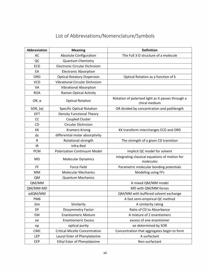
List of Abbreviations/Nomenclature/Symbols

Abbreviation Meaning Definition

AC Absolute Configuration The Full 3-D structure of a molecule

QC Quantum Chemistry

ECD Electronic Circular Dichroism

EA Electronic Absorption

ORD Optical Rotatory Dispersion Optical Rotation as a function of λ

VCD Vibrational Circular Dichroism

VA Vibrational Absorption

ROA Raman Optical Activity

OR, α Optical Rotation Rotation of polarized light as it passes through a

chiral medium

SOR, [α] Specific Optical Rotation OR divided by concentration and pathlength

DFT Density Functional Theory

CC Coupled Cluster

CD Circular Dichroism

KK Kramers-Kronig KK transform interchanges ECD and ORD

Δε differential molar absorptivity

R Rotational strength The strength of a given CD transition

IR Infra-Red

PCM Polarization Continuum Model Implicit QC model for solvent

MD Molecular Dynamics integrating classical equations of motion for

molecules

FF Force Field Parametric molecular bonding potentials

MM Molecular Mechanics Modeling using FFs

QM Quantum Mechanics

QM/MM A mixed QM/MM model

QM/MM-MD MD with QM/MM forces

adQM/MM QM/MM with buffered solvent exchange

PM6 A fast semi-empirical QC method

Sim Similarity A similarity rating

DF Dissymmetry Factor Ratio of CD to Absorbance

EM Enantiomeric Mixture A mixture of 2 enantiomers

ee Enantiomeric Excess excess of one enantiomer

op optical purity ee determined by SOR

CMC Critical Micelle Concentration Concentration that aggregates begin to form

LEP Lauryl Ester of Phenylalanine A surfactant

EEP Ethyl Ester of Phenylalanine Non-surfactant

xiii

LET Lauryl Ester of Tyrosine A surfactant

TAR12 Lauryl Ester Tartaric acid derivative

FLNa FMOC-Leucine A surfactant

PME Particle Mesh Ewald MD method for calculating long range electrostatics

ppm parts per million

VDF Vibrational Dissymmetry Factor Ratio of VCD/VA

EDF Electronic Dissymmetry Factor Ratio of ECD/EA

CID Circular intensity difference ROA/Raman

BN Binaphthol [1,1′-Binaphthalene]-2,2′-diol

DBBN Dibromobinaphthol 6,6'-dibromo-[1,1′-binaphthalene]-2,2′-diol

CSA2 Chiral Sulfonic Acid #2

EC Exciton Chirality Empirical CD theory

SpA spiroindicumide A diacetate

SpB spiroindicumide B diacetate

DEC Degenerate Exciton Chirality

NDEC Non-Degenerate Exciton Chirality

1

Chapter 1 Introduction

Any object that is not superimposable on its mirror image is said to be chiral. Most of the

compounds that comprise living organisms possess chirality, giving any chiral substance a different

response from its mirror image, which is called its enantiomer. To study the interactions of any chiral

molecule with a biological system, it is therefore important to know and understand molecular chirality,

made evident by the tragic case of thalidomide.1 But a pair of enantiomers have, as far as we can

measure, the same physical properties and can only be distinguished by reference to a known chiral

system, which could be light or the olfactory receptors in your nose.2 Since it is easier to construct

instruments that emit and measure light, that is the route that modern chemists, physicists, and

biologists have taken to study molecular chirality. Thus we will begin this work, diving into the world of

chiroptical spectroscopy: the measurement of the interaction of light with a chiral systems.

But the power to discriminate the two enantiomers of a chiral compound is not enough, at least

for the FDA, as one needs to know the 3-dimesional structure exactly, called the Absolute Configuration

(AC). Fortunately, it seems that the interactions of light with chiral substances can be reasonably

approximated using modern quantum chemical techniques,3-4 and with the combination of chiroptical

techniques and Quantum Chemistry (QC) calculations the exact 3-D structure of most small molecules

can be reliably determined. We will not stop there, since it is the structure that gives rise to the

chiroptical properties, the chiroptical properties can be informative on how a molecular system is

changing.5-8

The currently available spectroscopic tools in the exploration of chirality for molecular systems

include electronic circular dichroism (ECD), optical rotatory dispersion (ORD), vibrational circular

dichroism (VCD), Circularly Polarized Luminescence, and vibrational Raman optical activity (ROA). Each

has its own advantages and disadvantages such as useable solvents, concentration ranges, collection

times, sensitivities, etc. The techniques that will be used in this work will be discussed in the sections to

follow.

Optical Rotatory Dispersion (ORD) Optical Rotation (OR or α), discovered by Biot in 1812, is the rotation of the plane of polarization of

electromagnetic radiation as it passes through a medium.3, 9 OR is distinct from birefringence in that it

does not alter the polarization state of the beam. If the light rotates clockwise as it approaches the

observer, the sample is called dextrorotatory and OR is defined to be positive, while negative or

counterclockwise rotations come from levorotatory samples, which is a distinction used to label all chiral

compounds as (+) or (‒). The characteristic Specific Optical Rotation (SOR or [α]) is a widely used method

for differentiating between chiral molecules, and is generally written as,

lC

T

( 1-1 )

2

Where α is the observed rotation in degrees, λ is the wavelength of light in nm, T is the temperature, C is

the concentration in g/ml, and 𝑙 is the path length in dm. SOR should be independent of concentration,

but in some cases it has been found to vary slightly with concentration.10 The standard units of SOR are

𝑑𝑒𝑔 𝑚𝑙 𝑔−1𝑑𝑚−1. SOR changes with the wavelength of light, which is an effect called Optical Rotary

Dispersion (ORD). ORD was first calculated within the static limit in 1997, but these calculations are only

valid far from electronic transitions.11 ORD can be calculated using linear response theory for any given

wavelength and gives accurate results in most cases with Density Functional Theory (DFT) but the gold

standard is Coupled Cluster (CC) theory.12,13 ORD is calculated from the imaginary part of the electric

dipole-magnetic dipole polarizability (called the G’ tensor), which complicates the calculation of ORD

(and other chiroptical properties) by the origin dependence of the magnetic dipole moment operator.12

To obtain origin independent results, Gauge-Invariant (Including) Atomic Orbitals or the velocity gauge

must be used.14

OR is observed because left and right handed circularly polarized light travel at different speeds

in a chiral medium. Since linearly polarized light can be written as the sum of equal amounts of right and

left circularly polarized light, a difference in speed manifests as a change in the polarization angle. The

difference in refractive index is related to difference in absorption of left and right handed circularly

polarized light also called Circular Dichroism (CD). They are the real and imaginary parts of the complex

wave vector of light, and as a real complex pair they are interchangeable through the Kramers-Kronig

(KK) transformations. The relationship of the real and imaginary parts of a complex linear response

function f are related by:15

d

ff

0 22

Im2Re and ( 1-2 )

d

ff

0 22

Re2Im , ( 1-3 )

Where Re stands for the real part, Im stands for the imaginary part, and μ is a variable used for the

integration. The form of the KK relations makes ORD a long ranged effect when compared to CD and can

be measured for chiral compounds for which the ECD cannot be measured due to instrumental

restrictions. ORD can be measured routinely for any sample or solvent that does not significantly absorb

light at the wavelengths of interest. Rotations as small as 0.003 degrees can be measured and there is

no instrumental restriction on how large the angle of rotation can be.

Electronic Circular Dichroism (ECD) Circular Dichroism (CD) is the differential absorption of left and right handed circularly polarized

light. CD was discovered by the, then 26-year-old Ph.D. student, Aimé Cotton in 1895.16 In relation to the

Beer-Lambert law, the differential molar absorptivity (Δε) is defined by,

Cl

A

Cl

AA RLRL

( 1-4 )

Where l is the pathlength in cm, or length that the light beam passes through the sample, and C is the

concentration in mol L-1. ECD measures the differential absorption of left and right handed circularly

3

polarized light for electronic transitions observed in the UV-Visible spectral region. ECD is different for

Electronic Absorption (EA) in that it can be positive or negative. The strength of a given ECD transition is

characterized by the rotational strength (R), given by:17

dxR

40109422. ( 1-5 )

Where is the wavelength of the light in nm and the units of R are esu2cm2. The strength of a given

electronic transition can be calculated by the relation,18

kimikemek ikkiR ,, μμμμ ImIm ( 1-6 )

Where the transition goes from state i to state k , and μe and μm are the electric and magnetic

dipole moment operators respectively. For electronic transitions, theoretical spectral simulations are

normally carried out with Gaussian spectral intensity distribution, given as,

20

0

G

k

w

xx

kk eyxG

( 1-7 )

Where xk0 is the wavelength at the center of kth band, wG represents half-width at 1/e of the band

maximum.

Vibrational Circular Dichroism (VCD) Vibrational transitions can absorb right and left handed light differently giving rise to VCD.

However for vibrational transitions, the CD is approximately 10,000 times weaker than the Vibrational

Absorption (VA) of linear light, meaning there are inherent problems with noise when measuring VCD.

Due to the weakness of the VCD signal and other instrumental difficulties, measurements of VCD were

not performed until 1974.19 The removal of the linear birefringence signal20 has improved the reliability

of VCD measurements in newer instruments,21 which can reliably measure from 4000-800 cm-1. This

range allows for the observation of a large number of vibrational transitions, which can be compared to

QC calculations.

There are practical limitations on VCD measurements. Measurements of VCD are most easily

made in the solution phase, but nearly all solvents will absorb light in the Infra-Red (IR) region.

Deuterated solvents and short pathlengths (50-200 μm) must be used to minimize solvent absorbance.

To maximize the signal from the sample, high concentrations must be used which can lead to

aggregation effects. Also the sample may not dissolve at high concentrations in all solvents, and if

hydrogen bonding solvents are necessary, then the vibrations of the molecule will be perturbed by

hydrogen bonds with the solvent. The solvent interactions must be accounted for in comparisons with

QC calculations, which can alter the results significantly.22 VCD measurements on finely dispersed solid

particles and films can be made, but these require a rotating sample holder to remove linear dichroism

and the effects of strain on the sample.23

In spectral simulations, the vibrational absorption bands are generally represented by

Lorentzian band shapes given by,24

4

202

20

kL

Lkk

xxyxL

( 1-8 )

where γL is the half-width at half-maximum for the Lorentzian band and yk° is the peak y-value at xk°.

Quantum Chemistry (QC) For most typical organic molecules, their structure and properties can be calculated reliably

using Density Functional Theory (DFT).15 DFT can provide accurate results in most cases by empirically

accounting for electron correlation, and by fitting parameters to experimental data.25 The density

functional of choice in our lab is typically B3LYP, which includes Hartree-Fock character as well as

Becke’s exchange26 and correlation parametrized by Lee, Yang, and Parr.27 DFT methods can be used to

calculate the properties of molecular systems up to a few hundred atoms. In some cases28 DFT does not

properly model the electronic structure of the molecule and Coupled Cluster (CC) methods are

necessary,4, 29-34 but CC methods are practically limited to molecules with less than 20 2nd-row atoms.

To calculate the properties of a molecule, first all possible conformations, or different 3-D

arrangements of a given structure obtained by rotating about molecular bonds, are found by a search

algorithm. Then the structures of each of the conformations are optimized, or the bond lengths, bond

angles, and dihedral angles are altered until the minimum of energy is found. From the optimum

energies of the conformers, the one with the lowest energy is selected as the dominant conformation,

and any conformations with energies higher than a given cutoff are eliminated. The cutoff depends

upon the relative accuracy of the method used (~2 kcal/mol for DFT methods).35 All conformations that

have energies within the cutoff are used in the calculation of molecular properties. To obtain the time

average of a given spectra, the individual spectra from relevant conformers are Boltzmann weighted

according to the formula,

a

RTE

RTE

tot

ii

a

i

e

e

N

NP

/

/

( 1-9 )

Where Ei is the energy of a given conformation, R is the gas constant, and T is the temperature.

The effects of the solvent on the solute can be accounted for quickly by the use of continuum

models, with the model of choice being the Polarization Continuum Model (PCM).36 In the PCM, the

solute is surrounded by a dielectric medium with a spacing between the molecule and the dielectric

medium given by an empirical force field. PCM can provide a reasonable model for solvation by less

polar solvents but may fail to model hydrogen bonding solvent effects.37

Molecular Dynamics (MD) Molecular Dynamics (MD) is a computer simulation of the time evolution of a system of

interacting atoms or molecules. MD solves for the time evolution of the system by numerically

integrating classical equations of motion. MD is generally used with empirically fit molecular mechanics

(MM) force constants/parameters to calculate forces on atoms and to account for atomic interactions.

These parameters have been previously compiled and generalized into sets of force-fields (FF), and

contain coefficients for simple, predefined functions to recreate bonding potentials, Van der Waals, and

5

coulombic interactions. However, the MM energies can be off by several kcal/mol, such that MD

sacrifices accuracy for speed.38 The need for faster evaluation of forces is obvious: to perform accurate

integration, a maximum time step of 2 to 3 fs can be used. The simulations must be run for 1-1000 ns

depending upon the sampling needed, and therefore the method will require 500,000 – 500,000,000

force evaluations for the entire system. Other methods to compute the forces for the system include

semi-empirical NDDO, HF, DFT, and post-Hartree-Fock methods, though they may take orders of

magnitude longer to perform.25, 39-44

There has been a growing trend for the use of semi-empirical or simplified DFT methods to perform

the MD.45-47 The use of semi-empirical methods are generally thought to be not as reliable as some

other methods, but in this case they are the only QC methods fast enough to produce informative data.

In these calculations the size of the quantum mechanical system can be restricted to an important/core

region to save time, while bulk solvent is modeled with MM, which is called QM/MM (QM stands for

Quantum Mechanics). When MD is performed with the QM/MM method it is called QM/MM-MD. Some

solvent molecules can also be included in the QM region with variable solvent QM/MM-MD, where the

solvent molecule are allowed to flow into and out of the QM region, and since the forces are not

continuous at the boundary, force buffered/smoothing strategies have been developed,48-50 although

some implementations have lacked this feature.51

The sampling and size advantages of MD driven with MM or fast QM forces can be combined

with more accurate QC methods. The coordinates at regular intervals are exported, called a snapshot,

for an important subset of atoms/molecules and used for higher level calculations. Molecules deemed

less important (exterior to the core system) such as solvent, counterions, and other solute molecules

can be removed or kept as point charges for an explicit model of solvation. It is important to note that

water forms a semi-regular hydrogen bonding lattice as a liquid, and altering the level of calculation

used may interfere with the complex solvent-solute equilibria.

Similarity Methods The assessment of agreement between experimental and calculated chiroptical spectra has

been achieved mostly with a visual comparison between the two. When the spectra are composed of a

few well resolved bands this visual analysis is by far the easiest approach. But more often than not, VCD

and ROA, and sometimes also ECD, spectra contain several overlapping spectral bands. In such cases

experimental and calculated spectra are placed one above the other and correlations are drawn

between the observed spectral bands and simulated bands in the calculations. At times, such visual

analysis can be biased by personal judgments. Then the resulting configuration/conformation

assignments will inherit uncertainties, more than what one would have preferred. In such cases, one

legitimate question posed relates to the measure of agreement between experimental and calculated

chiroptical spectra.

Several methods have been developed to quantitatively determine the agreement between

experimental and calculated chiroptical spectra. In 2003 Bultinck and coworkers introduced a

dimensionless spectral overlap integral as a numerical measure of similarity52 in the experimental and

computed spectra. Bultinck extended this similarity measure, which was called the enantiomeric

similarity index, and developed a numerical measure of confidence in the calculated spectrum.53 Since

the methods developed by Bultinck involve some manipulation of the data, our lab has chosen to use a

similarity method developed by Shen et al, given as follows,54

6

fgggff

fg

III

ISimVA

( 1-10 )

fgggff

fg

III

ISimVCD

( 1-11 )

and

dxxgxfI fg ( 1-12 )

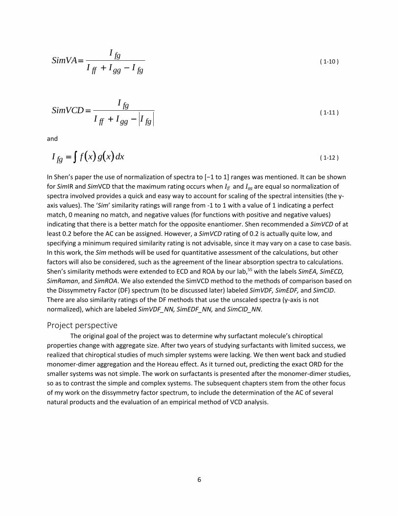
In Shen’s paper the use of normalization of spectra to [−1 to 1] ranges was mentioned. It can be shown

for SimIR and SimVCD that the maximum rating occurs when Iff and Igg are equal so normalization of

spectra involved provides a quick and easy way to account for scaling of the spectral intensities (the y-

axis values). The ‘Sim’ similarity ratings will range from -1 to 1 with a value of 1 indicating a perfect

match, 0 meaning no match, and negative values (for functions with positive and negative values)

indicating that there is a better match for the opposite enantiomer. Shen recommended a SimVCD of at

least 0.2 before the AC can be assigned. However, a SimVCD rating of 0.2 is actually quite low, and

specifying a minimum required similarity rating is not advisable, since it may vary on a case to case basis.

In this work, the Sim methods will be used for quantitative assessment of the calculations, but other

factors will also be considered, such as the agreement of the linear absorption spectra to calculations.

Shen’s similarity methods were extended to ECD and ROA by our lab,55 with the labels SimEA, SimECD,

SimRaman, and SimROA. We also extended the SimVCD method to the methods of comparison based on

the Dissymmetry Factor (DF) spectrum (to be discussed later) labeled SimVDF, SimEDF, and SimCID.

There are also similarity ratings of the DF methods that use the unscaled spectra (y-axis is not

normalized), which are labeled SimVDF_NN, SimEDF_NN, and SimCID_NN.

Project perspective The original goal of the project was to determine why surfactant molecule’s chiroptical

properties change with aggregate size. After two years of studying surfactants with limited success, we

realized that chiroptical studies of much simpler systems were lacking. We then went back and studied

monomer-dimer aggregation and the Horeau effect. As it turned out, predicting the exact ORD for the

smaller systems was not simple. The work on surfactants is presented after the monomer-dimer studies,

so as to contrast the simple and complex systems. The subsequent chapters stem from the other focus

of my work on the dissymmetry factor spectrum, to include the determination of the AC of several

natural products and the evaluation of an empirical method of VCD analysis.

7

Chapter 2 The ORD of aggregating systems much simpler than

surfactants

Some of the work presented in this chapter may be found in the PhysChemChemPhys article56

“Wavelength resolved specific optical rotations and homochiral equilibria” and the Chirality article57

“Specific Optical Rotations and the Horeau Effect”.

Introduction With the ultimate goal of understanding how and why the chiroptical properties of surfactants

change with aggregation, we will first consider the simplest aggregating system, that of a molecule

exhibiting monomer-dimer equilibrium. A more in-depth derivation of the equations can be found in the

literature.56

When molecules contain hydrogen bonding groups, there may be a preference for self-

association over interactions with solvent. The equilibrium expression for two monomeric units forming

a dimer is,

2

m

d

C

CK ( 2-1 )

where, Cm and Cd are, respectively, the molar concentrations of monomer and dimer (that include all of

the respective conformers). Using the material balance dmo CCC 2 , where Co is the molar

concentration of the prepared solution, and solving the resulting quadratic equation yields

omm CPC , where,

o

mKC

P811

2

( 2-2 )

The expression for Cd is obtained as, 𝐶𝑑 = 𝑃𝑑𝐶0, where 𝑃𝑑 is given as:

;811

811

2

1

o

o

dKC

KCP

( 2-3 )

Note that Pm and Pd cannot be termed mole fractions because they do not add up to one. Instead,

12 dm PP ( 2-4 )

and Pm and Pd are related to the mole fractions, xm and xd, respectively of monomer and dimer, as

8

m

m

d

m

dm

m

dm

mm

P

P

P

P

PP

P

CC

Cx

1

2

1

( 2-5 )

m

d

d

d

m

m

dm

d

dm

dd

P

P

P

P

P

P

PP

P

CC

Cx

1

2

11

1

( 2-6 )

For chiral systems undergoing equilibria, detailed experimental and theoretical SOR studies are

lacking in the literature.58 In one study, experimental OR studies at a single wavelength on systems at

equilibrium were suggested to be useful for determining the equilibrium constants.59 But the SORs of

equilibrating species and comparison to corresponding quantum chemical predictions were not

addressed. In a different study, quantum chemical predictions of SOR at a single wavelength for

monomer and dimer molecules were used to simulate the SOR for a system at equilibrium and the result

compared to the corresponding experimental SOR measurement at that wavelength, although the

adhoc equation used therein for SOR was incorrect.60

These literature studies point to multiple areas that are in need of new developments for

homochiral (only 1 enantiomer) species in equilibrium: (a). fundamental equations governing the SORs

remain to be established; (b). systematic experimental studies on wavelength resolved SORs for deriving

the molecular properties of species involved in equilibrium are lacking; (c). The reliability of modern

quantum chemical predictions of wavelength resolved SORs of equilibrating species remains to be

established.

Derivation of SOR for a Homochiral monomer-dimer mixture The system is complicated by the presence of the opposite enantiomer, so therefore we will

derive the relationships for the homochiral case, meaning only one enantiomer is present in solution.

Assuming that SORs of monomer and dimer are independent of concentrations, the observed OR, α, for

a pure enantiomeric substance exhibiting homochiral monomer-dimer equilibrium, can be written as

follows:

lMC

lMC

lclc ddd

mmmddmm

10001000

( 2-7 )

where [α]m and [α]d are the SORs, respectively of monomer and dimer species; l is the path length of the

cell used for OR measurement; cm is the concentration of monomer in g/cc; cd is the concentration of

dimer in g/cc; Mm is the molar mass of monomer; Md is the molar mass of dimer. Note that upper case

letter “C” is used for concentrations in mol L-1 units and lower case letter “c” is used for that in g cc-1

units.

Using the relations for Pm and Pd and accounting for the masses Md=2Mm, Eq ( 2-7 ) can be

modified as:

lMC

PP moddmm

10002

( 2-8 )

Writing the starting concentration, co, in g/cc of enantiomeric substance as,

9

1000

moo

MCc

( 2-9 )

the SOR of solution,

lco

( 2-10 )

becomes:

dmmm PP 1 ( 2-11 )

Eq. ( 2-11 ) is the fundamental expression for SOR of homochiral system exhibiting monomer-

dimer equilibrium. This equation can be seen to have the correct limiting values as follows: (a). As Co

approaches zero, Pm approaches 1 (see Eq. 5), and [α] becomes [α]m. (b). As Co approaches infinity, Pm

approaches 0, and [α] becomes [α]d. (c). For the special case of [α]m = [α]d, monomer-dimer equilibrium

should not influence the [α] of solution, which should then be independent of concentration Co, as

supported by Eq. ( 2-11 ). This equation is different from the one derived by Goldsmith et. al., which was

given as:60

ddmmEquil

22 ( 2-12 )

Which does not have the correct behaviour for the special case of [α]m = [α]d, and therefore cannot be

correct equation to describe the SOR at any arbitrary values of [α]m and [α]d.

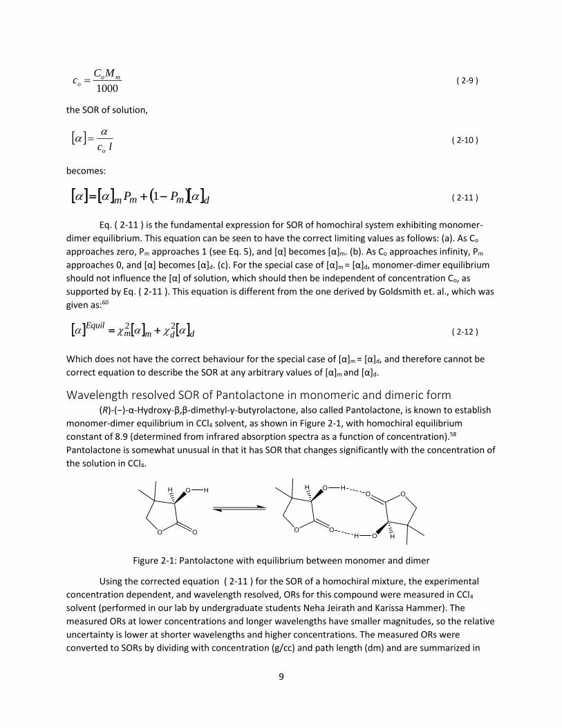
Wavelength resolved SOR of Pantolactone in monomeric and dimeric form (R)-(−)-α-Hydroxy-β,β-dimethyl-γ-butyrolactone, also called Pantolactone, is known to establish

monomer-dimer equilibrium in CCl4 solvent, as shown in Figure 2-1, with homochiral equilibrium

constant of 8.9 (determined from infrared absorption spectra as a function of concentration).58

Pantolactone is somewhat unusual in that it has SOR that changes significantly with the concentration of

the solution in CCl4.

Figure 2-1: Pantolactone with equilibrium between monomer and dimer

Using the corrected equation ( 2-11 ) for the SOR of a homochiral mixture, the experimental

concentration dependent, and wavelength resolved, ORs for this compound were measured in CCl4

solvent (performed in our lab by undergraduate students Neha Jeirath and Karissa Hammer). The

measured ORs at lower concentrations and longer wavelengths have smaller magnitudes, so the relative

uncertainty is lower at shorter wavelengths and higher concentrations. The measured ORs were

converted to SORs by dividing with concentration (g/cc) and path length (dm) and are summarized in

10

Table 2-1. These data can be used with Eq ( 2-11 ), along with reported K value of 8.958 to determine the

wavelength resolved SORs of monomer and dimer, []m and []d, respectively. Since the experimentally

measured property is the of solution, while the least squares fit is done for [], the weighted non-

linear least squares method61 is required to fit the data to Eq. ( 2-11 ). The weights for individual SOR

values were determined through error propagation using uncertainties in observed ORs, and in

concentrations of solutions. In a simpler method, weights were determined assuming that relative

errors in concentrations are smaller than those in ORs. Both approaches yielded identical values for [α]m

and [α]d within their associated errors and weighted higher concentration data more than those at

lower concentrations.

Conc (mM) [α]633 [α]589 [α]546 [α]436 [α]405 [α]365

1.94 -4.37 -3.57 -5.56 -36.90 -20.63 -51.59

4.12 -5.04 -7.46 -11.01 -25.00 -37.50 -52.24

6.09 -4.42 -7.32 -10.10 -25.76 -36.36 -60.61

8.05 -5.53 -7.06 -10.78 -26.72 -39.31 -68.23

12.05 -6.70 -9.69 -11.35 -30.55 -40.82 -70.47

15.12 -7.88 -10.26 -12.65 -32.06 -44.41 -72.46

23.02 -9.61 -12.35 -15.52 -37.05 -49.03 -82.04

38.36 -12.06 -14.90 -19.37 -42.45 -57.69 -94.11 Table 2-1: Measured SOR values for (R)-(−)-pantolactone in CCl4

The fits were performed using the Kaleidagraph program; the results obtained from the fits for

[α]m and [α]d are summarized in Table 2-2 in deg cm2 g-1 dm-1 units. This is the first determination of

wavelength resolved [α]m and [α]d for a chiral enantiomer at homochiral equilibrium.

nm []m error []d error

633 -0.5 0.6 -36.0 1.6

589 -1.3 0.7 -43.9 1.7

546 -2.7 0.6 -54.6 1.7

436 -8.8 1.6 -112.9 4.2

405 -18.3 2.2 -139.9 5.9

365 -37.4 2.7 -212.5 7.2 Table 2-2: Fitted SOR values of the (R)-(−)-pantolactone monomer and dimer in CCl4

Calculated SOR for the pantolactone monomer and dimer It is a useful benchmark to compare the experimental values of the wavelength resolved SOR of

the monomer and dimer form of pantolactone with the values calculated using DFT. To that end, a

computational study of the pantolactone system was undertaken. Conformational analysis confirmed

four low energy conformations for dimer and two low energy conformations for monomer as reported

in the literature.60 These conformations are used as the starting point for further geometry

optimizations and SOR calculations. Though CCl4 is a non-polar solvent, solvents effects were

nevertheless included with the PCM. The populations, at B3LYP/Aug-cc-pVTZ/PCM level, of two

monomer conformers are 97% and 3%, while those of four dimer conformers are 91%, 5%, 2% and 2%.

11

Thus in essence, there is only one predominant conformer each for monomer and dimer. Dispersion

corrected DFT, and also the M06-2X functional (which has been parametrized incorporating non-

covalent interactions),62 confirmed this conclusion. Additional calculations were also undertaken for the

dominant dimer conformer at various levels of theory, and were seen to have little effect on the

calculated SOR values.

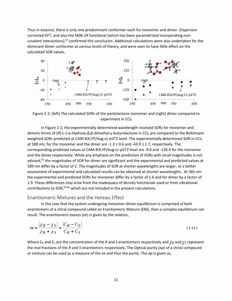
Figure 2-2: (left) The calculated SORs of the pantolactone monomer and (right) dimer compared to

experiment in CCl4

In Figure 2-2, the experimentally determined wavelength resolved SORs for monomer and

dimeric forms of (R)-(−)-α-Hydroxy-β,β-dimethyl-γ-butyrolactone in CCl4 are compared to the Boltzmann

weighted SORs predicted at CAM-B3LYP/Aug-cc-pVTZ level. The experimentally determined SOR in CCl4

at 589 nm, for the monomer and the dimer are -1.3 ± 0.6 and -43.9 ± 1.7, respectively. The

corresponding predicted values at CAM-B3LYP/Aug-cc-pVTZ level are -9.6 and -128.4 for the monomer

and the dimer respectively. While any emphasis on the prediction of SORs with small magnitudes is not

advised,63 the magnitudes of SOR for dimer are significant and the experimental and predicted values at

589 nm differ by a factor of 2. The magnitudes of SOR at shorter wavelengths are larger, so a better

assessment of experimental and calculated results can be obtained at shorter wavelengths. At 365 nm

the experimental and predicted SORs for monomer differ by a factor of 1.6 and for dimer by a factor of

1.9. These differences may arise from the inadequacy of density functionals used or from vibrational

contributions to SOR,64-66 which are not included in the present calculations.

Enantiomeric Mixtures and the Horeau Effect In the case that the system undergoing monomer-dimer equilibrium is comprised of both

enantiomers of a chiral compound called an Enantiomeric Mixture (EM), then a complex equilibrium can

result. The enantiomeric excess (ee) is given by the relation,

SR

SR

SR

SR

CC

CCee

( 2-13 )

Where CR and CS are the concentration of the R and S enantiomers respectively and χR and χS represent

the mol-fractions of the R and S enantiomers respectively. The Optical purity (op) of a chiral compound

or mixture can be used as a measure of the ee and thus the purity. The op is given as,

12

pure

emop

( 2-14 )

The op and the ee are equal in ideal situations, however the op can be different from the ee in some

cases as shown by Horeau in the 1960s.67-68 The situation when the op and the ee of an EM are not equal

has been given the term “The Horeau effect” shown in Figure 2-3, however it has only been measured in

a handful of cases, shown in Figure 2-4.

Figure 2-3: The Horeau effect in 2-methyl-2-ethyl succinic acid, shown op vs ee67

Figure 2-4: Compounds that exhibit the Horeau effect67-70

Chiral aggregation is considered to be the source of the Horeau effect.71-72 But even though the

Horeau effect has been known for almost five decades, the conditions under which it may, or may not,

be observable are not established. To resolve this issue, we will derive the expressions for the SOR of an

EM exhibiting homochiral and heterochiral monomer-dimer equilibria and investigate how the op and

the ee are related. A more in-depth derivation can be found in the literature .57

13

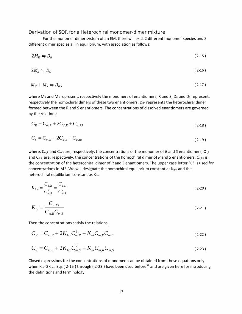
Derivation of SOR for a Heterochiral monomer-dimer mixture For the monomer dimer system of an EM, there will exist 2 different monomer species and 3

different dimer species all in equilibrium, with association as follows:

2𝑀𝑅 ⇋ 𝐷𝑅 ( 2-15 )

2𝑀𝑆 ⇋ 𝐷𝑆 ( 2-16 )

𝑀𝑅 + 𝑀𝑆 ⇋ 𝐷𝑅𝑆 ( 2-17 )

where MR and MS represent, respectively the monomers of enantiomers, R and S; DR and DS represent,

respectively the homochiral dimers of these two enantiomers; DRS represents the heterochiral dimer

formed between the R and S enantiomers. The concentrations of dissolved enantiomers are governed

by the relations:

RSdRdRmR CCCC ,,, 2 ( 2-18 )

RSdSdSmS CCCC ,,, 2 ( 2-19 )

where, Cm,R and Cm,S are, respectively, the concentrations of the monomer of R and S enantiomers; Cd,R

and Cd,S are, respectively, the concentrations of the homochiral dimer of R and S enantiomers; Cd,RS is

the concentration of the heterochiral dimer of R and S enantiomers. The upper case letter “C” is used for

concentrations in M-1. We will designate the homochiral equilibrium constant as Khm and the

heterochiral equilibrium constant as Kht.

2

,

,

2

,

,

Sm

Sd

Rm

Rd

hmC

C

C

CK ( 2-20 )

SmRm

RSd

htCC

CK

,,

, ( 2-21 )

Then the concentrations satisfy the relations,

SmRmhtRmhmRmR CCKCKCC ,,

2

,, 2 ( 2-22 )

SmRmhtSmhmSmS CCKCKCC ,,

2

,, 2 ( 2-23 )

Closed expressions for the concentrations of monomers can be obtained from these equations only

when Kht=2Khm. Eqs ( 2-15 ) through ( 2-23 ) have been used before59 and are given here for introducing

the definitions and terminology.

14

Iterative solutions to Eqs. ( 2-22 ) and ( 2-23 ) can be obtained when Kht ≠ 2Khm, by starting with

the values of Cm,R and Cm,S when Kht=0 repeatedly solving the quadratic form of the equilibrium

expressions until the values do not change. In general the SOR of an EM can be determined once the

concentrations and SORs of all the substituents are known from the equation:

SdRdRdSmRmRmo

EM CCCCC

,,,,,, 21 ( 2-24 )

Note here that the heterochiral dimer is not in the equation, because it cannot contribute to the net OR

for reasons of symmetry. Either the heterochiral dimer is not chiral or there will be equal amount of

both enantiomers of the heterochiral dimer. Some cases of the theoretical monomer-dimer Horeau

effect are shown in Figure 2-5.

Figure 2-5: Some examples of the exact solution of the monomer-dimer Horeau equations

Special Case: Kht=2Khm The values of Kht=2Khm is a common occurrence for aggregating chiral monomer-dimer

molecules. In this situation, the combination of Eqs ( 2-22 ) and ( 2-23 ) gives,

02 ,,

2

,, SRSmRmSmRmhm CCCCCCK ( 2-25 )

and is mathematically equivalent to the homochiral case. Both enantiomers will be described by the

same Pm relationship to the starting concentration and will have the same ratio of monomer and dimer

units. The op will change linearly with ee, and in this case the Horeau effect will not be observed.

Special Case: [α]m = [α]d If the formation of the dimer does not significantly perturb the monomer so as to change its

SOR, the SORs for the EM can be trivially derived from Eq ( 2-24 ) by adding and subtracting Cd,RS,

15

eeC

CC

CCCCCCC

Ro

SRR

RSdSdSmRSdRdRmo

REM

,,,,,, 22

( 2-26 )

In summary, when [α]m,R=[α]d,R or when Kht=2Khm no distinction can be made between op and ee,

and the Horeau effect will not be observed.

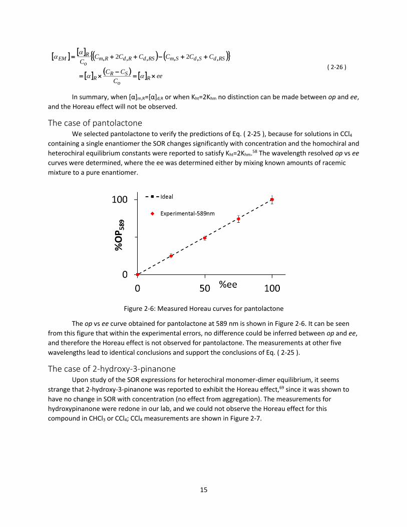
The case of pantolactone We selected pantolactone to verify the predictions of Eq. ( 2-25 ), because for solutions in CCl4

containing a single enantiomer the SOR changes significantly with concentration and the homochiral and

heterochiral equilibrium constants were reported to satisfy Kht=2Khm.58 The wavelength resolved op vs ee

curves were determined, where the ee was determined either by mixing known amounts of racemic

mixture to a pure enantiomer.

Figure 2-6: Measured Horeau curves for pantolactone

The op vs ee curve obtained for pantolactone at 589 nm is shown in Figure 2-6. It can be seen

from this figure that within the experimental errors, no difference could be inferred between op and ee,

and therefore the Horeau effect is not observed for pantolactone. The measurements at other five

wavelengths lead to identical conclusions and support the conclusions of Eq. ( 2-25 ).

The case of 2-hydroxy-3-pinanone Upon study of the SOR expressions for heterochiral monomer-dimer equilibrium, it seems

strange that 2-hydroxy-3-pinanone was reported to exhibit the Horeau effect,69 since it was shown to

have no change in SOR with concentration (no effect from aggregation). The measurements for

hydroxypinanone were redone in our lab, and we could not observe the Horeau effect for this

compound in CHCl3 or CCl4; CCl4 measurements are shown in Figure 2-7.

16

Figure 2-7: (left) Horeau effect previously reported69 in CHCl3 and (right) performed in our lab in CCl4

Apparently the Horeau effect previously reported was not correct, as supported by repeated

measurements and Eq. ( 2-26 ).

Figure 2-8: The concentration dependence of (1S,2S,5S)-(−)-2-hydroxy-3-pinanone in CCl4

The concentration dependent SOR values at 589 nm for (1S,2S,5S)-(−)-2-hydroxy-3-pinanone in

CCl4 are displayed in Figure 2-8. The SOR at 589 nm can be considered to be independent of

concentration, within the experimental errors, and no concentration dependence of SOR for

hydroxypinanone in CCl4 at other wavelengths was observed. To confirm that the molecules were in fact

aggregating, the homochiral equilibrium constants in CCl4 and CHCl3 were measured by concentration

dependent IR measurements with subsequent least-squares fitting, shown in Figure 2-9. The homochiral

equilibrium constant was determined to be 2.2 ± 0.5. Pm values at 100 mg/ml (0.6 M) and 3 mg/ml

(0.018 M) would then be 0.46 and 0.93 respectively, meaning there is a significant shift in the population

of monomer and dimer species over the concentration range of the measurements. Since it can be

confirmed that the species is aggregating, yet there is no observable concentration dependence of SOR,

hydroxypinanone is not expected to display concentration dependent SOR even in very dilute solutions.

17

Figure 2-9: IR O-H stretching region measurements on (1S,2S,5S)-(−)-2-hydroxy-3-pinanone in CCl4

Calculated SOR for (1S,2S,5S)-(−)-2-hydroxy-3-pinanone Since calculations on pantolactone could reasonably predict the SOR of the monomer and

dimer, the calculations were performed on hydroxypinanone. Conformations of monomer and dimer

units were built based on structures found from pantolactone, and verified by conformational searches

in MacroModel.73 The Boltzmann weighted ORD calculated at the B3LYP/6-311++G(2d,2p)/PCM level for

the monomer and the dimer are compared to the experimental in Figure 2-10. The calculated ORD for

the monomer matches very closely to the experimental values. Since experimental ORD values are

independent of concentration, the ORD values for the monomer and dimer should be equal. However,

the ORD of the dimer is calculated to be 3 times too large.

18

Figure 2-10: The calculated ORD for (1S,2S,5S)-(−)-2-hydroxy-3-pinanone at the B3LYP/6-

311++G(2d,2p)/PCM level compared to experiment in CCl4

The discrepancy in the calculated ORD for the dimer is puzzling, because IR measurements had

shown that aggregation does in fact occur. To gain more insight on the monomer-dimer system VCD

measurements were taken at 2 different concentrations, and using the equilibrium constant, the

experimental VCD spectrum of the monomer and dimer could be determined from the matrix equation,

2

1

1

2,2,

1,1,

dm

dm

d

m

PP

PP ( 2-27 )

Where 1 and 2 label measurements at different concentrations. VCD measurements over large

concentration ranges is not normally possible for most compounds, but hydroxypinanone (liquid at

room temperature) is soluble at high concentrations in CCl4, allowing for collection of VCD spectra over

a large wavelength region, shown in Figure 2-11.

19

Figure 2-11: The experimental VCD for both the monomer and dimer of (1S,2S,5S)-(−)-2-hydroxy-3-

pinanone in CCl4, arrows showing the bands most effected by aggregation

Figure 2-12: The VCD for both the monomer and dimer of (1S,2S,5S)-(−)-2-hydroxy-3-pinanone

calculated at the B3LYP/6-311++G(2d,2p) level

The calculated VCD for the monomer and dimer units can be used to judge the accuracy of the

model conformations, shown in Figure 2-12. VCD peaks that are altered by dimer formation at 1050,

1101, and 1350 cm-1 are well reproduced in the calculations. Since the calculations reasonably

reproduce the experimental VCD, we can conclude that our model for the dimer is accurate. Yet still the

ORD predicted for the hydroxypinanone dimer is not well calculated. The reason for this could be that

higher level calculations are needed to properly model the electronic structure of the dimer. Another

possibility is that the potential energy surface for the dimers is too broad to approximate the structure

of the dimer with a few optimized conformations. Further investigations are ongoing.

The case of 2-methyl-2-ethyl-succinic acid After investigating systems that exhibit monomer-dimer equilibrium, there are the cases of the

di-carboxylic acids, namely 2-methyl-2-ethyl-succinic acid and 2-isopropyl-2-methyl-succinic acid.67 The

dicarboxylic acids probably would not tend to form dimers, due to the angle between carboxyl groups.

The lowest energy conformation of the monomer of 2-methyl-2-ethyl-succinic acid is shown in Figure

2-13. The formation of trimers, tetramers, pentamers, etc. are energetically more favorable; an example

homochiral tetramer is shown in Figure 2-14. The existence of higher order aggregation equilibria in the

2-methyl-2-ethyl-succinic acid system could explain the reason for the observed Horeau effect, though

the expressions would be too complicated to solve analytically.

20

Figure 2-13: An optimized monomer unit of (S)-2-methyl-2-ethyl-succinic acid

Figure 2-14: An optimized homochiral tetramer unit of (S)-2-methyl-2-ethyl-succinic acid

There are many problems with this system that must be addressed, before calculations on this

system can be informative. Firstly there exists the possibility for trimers, tetramers, pentamers, etc. but

the equilibrium constants for each of these associations is not known. Also considering only the

tetramer system, there exist a rather large number of possible conformations, and to the author’s

current knowledge, there are no systematic conformational searching codes available for non-covalently

bound systems. The tetramer is already quite a large system to investigate computationally, and since

the monomers are not bonded covalently, the PES is broad and optimizations are tedious. To make

matters worse, the value of the SOR for the compound is not large, meaning the accuracy of QC SOR

calculations will be approximate.

To illustrate, both a 100,000 step and a 1,000,000 step random/Monte Carlo based

conformational search in MacroModel73 on the homochiral tetramer, produced ~1000 unique

structures. However, upon subsequent optimizations using the PM6 Hamiltonian, it was discovered that

21

new conformations could be generated by altering the dihedral angle of the ethyl group, and therefore

not all conformations were found by MacroModel.

Conclusion The observed SOR of a compound can be dependent upon the concentration of that compound

in solution. In the case of pantolactone, the effect comes from the formation of dimeric aggregates in

solution which can be described and modeled with QC calculations. For other compounds, such as

hydroxypinanone, aggregation is known to occur in solution, but the effect on the ORD is not well

understood or reproduced with QC calculations. Even though hydroxypinanone is a rigid compound,

even a simple dimeric system has proven to be too complicated to model with optimized structures and

DFT calculations. For cases of higher order aggregates, such as 2-methyl-2-ethyl-succinic acid, the

situation is complicated by the system size and the number of configurations.

It seems that even simple aggregating systems of dimers can have chiroptical properties that are

difficult to calculate exactly by QC methods. If the QC methods are extended to even more complex

aggregating systems like surfactants, we must accept that any results or conclusions are at best

qualitative. Nevertheless, QC calculations on such systems can be useful if the questions are asked in the

right way.

22

Chapter 3 The Chiroptical Properties of Surfactants

Introduction Surfactants are a class of compounds that are “surface active”, in that they tend gather at

surfaces between immiscible liquids and change the amount of work needed to expand the surface.74

Surfactants generally consist of two chemically distinct portions: a lyophilic group that favorably

interacts with the solvent and a lyophobic group that has little interaction with the solvent. The

presence of the lyophobic group in a solvent will disturb the liquid structure and raise the free energy of

the system, and this in turn means less work is needed to bring the surfactant to the surface. If enough

surfactant molecules are present in solution, then the surface free energy can be low enough for them

to aggregate and spontaneously create their own surface within the solvent. These clusters are called

micelles, and the concentration required to form micelles is called the Critical Micelle Concentration

(CMC).74-76 Micelles can take on different shapes and sizes, some of which are shown in Figure 3-1, and

in water their constituents generally share a charged/polar, lyophilic “head” and a long linear

hydrocarbon, lyophobic “tail”.

Figure 3-1: Some structures of aggregating surfactants

Recent experimental results from our laboratory have shown that chiroptical spectra of

surfactants can change depending upon the state of aggregation.77-79 The most dramatic change has

been seen in the specific rotation of chiral surfactants, which can become strongly dependent upon

concentration. Some of the key results are summarized below as the concepts are important for the

work to follow. The structures of the five key surfactant molecules discussed in this work are shown in

Figure 3-2.

23

Figure 3-2: Structures of some key surfactants in this work

A study on FLNa showed that the SOR of FLNa changed exponentially after the CMC, shown in

Figure 3-3.77,78 ECD studies did not reveal the formation of new bands, or disappearance of the initial

bands, in the CD or absorbance upon changing concentration. Therefore, it is possible that the observed

changes in SOR could be coming from the higher energy electronic transitions that could not be

experimentally investigated.

Figure 3-3: SOR and surface tension as a function of concentration for FLNa in water and methanol

In the case of TAR12, the SOR is seen to change more at some wavelengths than others, shown

in Figure 3-4.

24

Figure 3-4: SOR as a function of concentration for TAR12 in water, data from Raghavan Vijay (unpublished)

In the study of LEP, the SOR was correlated linearly to the aggregation number through

temperature controlled measurements as shown in Figure 3-5.79 The LEP study is very informative

because it establishes a theoretical basis with which hypotheses can be generated. The CMC of LEP was

found previously to be 0.13 mM.80

Figure 3-5: SOR of LEP and the aggregation number79

While the SOR appear to change linearly for LEP, for the compound LET the SOR is more affected

by temperature than the size of the aggregates, as shown in Figure 3-6. The comparison between LEP

and LET shows how a slight change in the surfactant head group can change the properties of the

surfactant and the chiroptical properties of the surfactant system. A previous NMR study has shown that

there are conformational differences in the head groups of aggregated LEP and LET surfactants,81

however there is no theoretical basis to distinguish their chiroptical behavior with regards to

concentration and temperature.

25

Figure 3-6: SOR of LET changing with aggregation number and temperature79

Surfactants are large and complex systems that are difficult to study experimentally and

computationally. If the relationships between concentration and SOR are to be understood from

quantum chemical calculations, there must first be a hypothesis that will be tested by the alteration of

the system parameters, and then comparison with experimental data will either confirm or reject the

theory. The change in SOR of chiral surfactants will be considered to come from 4 different effects of

aggregation:

1. Conformational changes in individual molecules: The populations of conformers may change

when the molecules aggregate together. Some bulky conformations may be disfavored for ones

that fit favorably.

2. Large scale chiral assembly: Chiral molecules can form large-scale chiral structures with

enhanced chiroptical properties.82

3. Electronic Coupling: Electronic coupling coming from the though-space interaction between

electric transition dipole moments in different chromophores83,84 could be important, as noted

in some solid state ECD studies. This effect is quite large and pair-wise interactions must be

considered.85

4. Electrostatic Environment: The ionic surfactants are all charged and gather together in numbers

of approximately 50 to 150. The localization of the charge and preferential orientation may

polarize some of the electronic transitions, which in turn can change the SOR.86

Each of these causes was investigated to determine to what extent they contribute to overall SOR of a

model chiral surfactant system.

Additional considerations for studies of surfactant systems is the concentration range over

which the system changes. The CMC of LEP is known to be 0.13 mM, however due to pathlength

restrictions, OR of LEP cannot be accurately measured for solutions below 1.5 mM. The ECD suffers the

opposite effect, such that the ECD of LEP cannot be measured on solutions above 67 mM, but can be

measured at concentrations as low as 6.4 μM.

26

ECD and ORD of LEP Considering pathlength restrictions for the ORD and ECD techniques, the experimental spectra

for LEP were collected in water over all measureable concentrations. The ORD of LEP is seen to increase with increasing concentration at all wavelengths, though with non-linear relationship to concentration, as shown in Figure 3-7 and Figure 3-8. With the new data plotted on a logarithmic scale, an approximately linear trend is observed, similar to the case of FLNa (see Figure 3-3).

Figure 3-7: ORD measurements on L-LEP in water

Figure 3-8: SOR for L-LEP as a function of concentration, linear and log scale

ECD measurements on the LEP system utilizing 5 cm to 10 μm pathlengths are shown in Figure

3-9. There are some apparent changes in the positive peak at 218 nm, with increasing ECD signal with

increasing concentration. Also the new ECD measurements of LEP include concentrations that were not

previously measured.

27

Figure 3-9: ECD measurements on LEP in water

It is also possible to determine the effect of the experimental ECD spectra on the observed ORD using the Kramers-Kronig (KK) transform.87 Comparing the KK transformed ECD to the observed ORD can reveal how much influence the ECD outside the observable range has on the measured ORD and can be used for comparative purposes (the KK transform only takes into account the observed ECD). The ORD derived from the KK transform are also displayed in Figure 3-10. The KK transformed ECD at 589 nm gives ORD values of 37 and 54 deg cc g-1 dm-1 for the ECD taken at 0.8 mM and 8 mM respectively. However the measured ORD for 7.8 and 1.5 mM solutions is 9.9 and 4.3 deg cm g-1 dm-1 respectively. Therefore the differences between these two sets must come from transitions outside of the measureable ECD range.

Figure 3-10: Observed ORD compared to KK-Transformed ECD

Signal limitations on LEP limit the practical concentration range of ORD measurement and prevent observation of the SOR of LEP before CMC. ECD measurements can be made below CMC, however they absorb too strongly at higher concentrations for accurate chiroptical measurements.

28

Computational Modeling of Surfactant Systems Since aggregated surfactant systems are large and complex, MD is used to simulate the

surfactant monomers and their environment either in an aqueous environment or as part of an aggregated structure.88-90 As for the structure of the aggregate, it is quite complicated to achieve sufficient sampling to observe phase changes or determine the preference of a particular surfactant. In these studies, all aggregates are constructed to be in a specific phase (mostly as micelles) and allowed to sample configurational space in that phase. First attempts were to use Kirkwood91 and Applequist92-93 semi-empirical methods to calculate the SOR from snapshots of TAR12 micellar aggregates, however the results showed no change with increasing size and furthermore did not predict the correct sign of the SOR. Attempts to use semi-empirical methods have been abandoned for the use of more accurate QC methods. However the QC methods require ~8000 times the CPU time as the semi-empirical methods (~2 CPU hours for 1 LEP monomer to calculate SOR at one wavelength using B3LYP/6-31G*). Using the MD snapshots, many QC calculations (100-1000) are necessary to get convergence in the average of the final property. QC methods also scale poorly with increasing system size making calculations on all but a few surfactant molecules impractical. To determine the sensitivity of the QC calculations to system computational parameters, a series of test calculations were performed on the EEP system, shown in Figure 3-11. The average SOR does not change significantly according to DFT, so the B3LYP/6-31G* level will be used for most calculations involving large numbers of snapshots. Error bars were taken to be the standard deviation in the mean.

Figure 3-11: SOR calculations on aqueous EEP system at various levels of theory, 625 snapshots for all

except the B3LYP/Aug-cc-pVDZ calculations which used 274 snapshots

Other considerations are needed when using raw, unmodified, snapshots from an MD trajectory

driven by MM forces. The geometries of the molecules in the snapshots will be distorted from the

equilibrium geometry. The distorted geometries may produce unrealistic excitation energies. When the

energy of the incident radiation is near an electronic excitation, traditional methods of SOR calculation

give spuriously high (resonant) SOR magnitudes. It is important to identify snapshots that are near

resonance, and handle them accordingly. A set of test calculations was performed on EEP snapshot

structures, by calculating SOR at many wavelengths, including those close to the true electronic

excitation of EEP (~220 nm). The electronic excitation energies are not calculated in SOR calculations,

29

but the HOMO-LUMO energy gap is calculated in the initial SCF procedure. From the HOMO-LUMO

energy gap, the first electronic excitation energy can be estimated.94 This threshold energy can be used

to determine near resonant values and exclude them from the average, as shown in Figure 3-12. With

resonant ORD values removed, the average SOR value is valid with the condition that the number of

snapshots removed is small. It can be shown that the unrealistic excitation energies come from the

distorted geometry of the molecules from the raw snapshots, because when the molecules are

optimized, resonant snapshots do not appear far from the true excitation energy. Data for molecules

optimized using the PM6 Hamiltonian prior to ORD calculation are also shown in Figure 3-12, which is to

show that even a fast semi-empirical method such as PM6 can produce reasonable geometries.

Figure 3-12: (left) Average ORD and (right) Average ORD excluding resonant snapshots for EEP

With test systems on EEP behaving normally, several MD simulations on LEP surfactant structures built with PACKMOL were performed using Amber12 GPU implementation using the GAFFLipid force field.95,96 The details on the MD simulations on the LEP and other surfactant systems are given in “Details on the MD simulations”.

Results and analysis

Calculations on electronic coupling effects To determine if the change in SOR was caused by electronic coupling, ORD calculations were

performed on multiple surfactant molecules extracted from MD trajectories. Since electronic coupling, if assumed to be of dipolar interaction type, scales as 1/r3, the closest surfactant molecules should have the most coupling, therefore pairs of two LEPs were extracted from a 40 molecule micelle based on the criterion that they have the smallest distance between their chiral carbon atoms. Additionally sets of 3 were based on the sum of the squares of the distances. Since the aliphatic tail portions have no chirality, they can be replaced with methyl groups to speed up the calculations and reduce the variance in the calculated SOR which may skew the average.

The results of calculations on 1, 2, and 3 LEP molecules with and without tails are shown in Figure 3-13. The difference in the average for a single LEP molecule with tails may be due to a size or sampling issue. Since no trend can be observed when the tails are removed, the calculations indicate that electronic coupling does not affect the SOR values upon aggregation and is therefore not responsible for the changing SOR values seen in LEP. The lack of a clear trend from the calculations was troubling at first, because of the significant changes in the measured SOR of several surfactants. It was originally thought that a strong coupling phenomenon such as exciton coupling would be the cause of

30

the changing SOR, but exciton coupling usually produce a pair of strong CD bands of opposite sign (called a couplet). If there was significant exciton coupling, it should be made apparent by changes in the ECD, which shows little change. Considering that there is no observable exciton coupling, it is not surprising that small clusters of LEP do not change the calculated SOR appreciably.

Figure 3-13: Trends in calculated SOR on LEP clusters, using B3LYP/6-31G*

Large scale chiral assembly Regarding the possibility for large scale chiral assemblies, transmission electron microscope experiments indicated that LEP forms spherical micelles,79 large scale chiral assemblies can be ruled out. Also the MD trajectories indicated that the surface of the aggregates is very dynamic and therefore unlikely to be able to form a supramolecular chiral structure. The lack of electronic coupling and large scale assembly can be rationalized by considering that the water molecules must solvate the charged groups and prevent any long range order and on average cancels out any coupling that may occur.

Figure 3-14: TEM images of LEP (left) 50 mM and (right) 200 mM79

LEP and the Horeau effect The Horeau effect explored first in the monomer-dimer case, can be used as an experimental

means of investigating the surfactant systems. In the monomer-dimer case, the Horeau effect was not observed when Kht=2Khm, or when [α]m = [α]d. For surfactants the argument can be made that the association constant for surfactants should not change for the opposite enantiomer, namely Kht≈Khm. This is because surfactants aggregate due to non-bonding interactions in the tail portion, which in this case is not chiral. Also it is safe to assume that the SOR of the monomer and aggregated forms of surfactant are different, since SOR changes with concentration.

31

The measurements of the SOR for 200 mM LEP at various ee’s were performed, shown in Figure 3-15. The data shows SOR is decreasing linearly with ee, and several interpretations can be made of it. That the Horeau effect is not observed in LEP, or that the two enantiomers of LEP do not mix in solution and remain is a semi-crystal state (as evidenced by the large structures seen in the microscopy experiments). Additional experiments have been performed on 50 mM LEP and at other temperatures with similar trends. The lack of a Horeau effect in LEP should then rule out the possibility for large scale chiral assemblies. Because if the surfactants mix evenly, large scale chiral structures would be disfavored.

For how the Horeau effect may manifest itself in electronic coupling is a more complicated matter, the details of which will be relegated to the appendices, see “The Horeau effect in aggregated systems and electronic coupling.” The current interpretation of the Horeau effect is that the electronic coupling does not contribute in a major way the SOR of LEP upon aggregation. An observation that supports the calculations. Though the calculations and lack of Horeau effect should not be considered definitive, we have a case against electronic coupling as a major factor in the SOR of LEP.

Figure 3-15: SOR of 200mM LEP as a function of ee at 25°C

Conformational Changes using Molecular Mechanics Force Fields To determine if the change in SOR upon aggregation was due to a change in conformational

populations, a thorough conformational analysis has been performed on the MD simulations. To determine the key dihedral angles principle component analysis was performed using all dihedral angles and the calculated SOR at 589 nm for a set of LEP molecules extracted from a 40 molecule micelle. The analysis indicated that only two dihedral angles are important to the average SOR: they control the relative angles of the two chromophores in the molecule, which would intuitively be the case (see Appendix A ). These angles are labeled φ and ψ and are shown in Figure 3-16.

32

Figure 3-16: The dihedral angles φ and ψ (bold indicating the atoms that define them), Carbonyl

chromophore also shown

The relative occupancy of the dihedral angles may change as the aggregates change and

produce alternate averages for the SOR observed in experiment. Analysis of the GAFFlipid MD

trajectories between different sized micelles indicates that the dihedral angles do change between

single LEP in water and several LEPs forming larger micelles, also shown in Figure 3-17. Integrating over

the histogram for the angle ψ produces a 10% difference in the dihedral populations between the two

simulations.

Figure 3-17: Histograms of the φ and ψ values in 1 and 40 LEP MD simulations

The GAFFlipid simulations indicate that the populations of the conformers change in aggregated

form, but only a 10 % change in one dihedral angle is not expected to produce dramatically different

SOR values, as shown below.

Electrostatic effects using Molecular Mechanics Force Fields To investigate the electrostatic contribution to SOR, the electric field at the carbonyl

chromophore (see Figure 3-16) from all other point charges was calculated from the MD snapshots for

each molecule. Generally the surfactant’s tail should point inward and the head group outward, so the

best way to center a coordinate system would be to use the bond vector from the carbonyl carbon to

the alpha carbon, made to be the z-axis as shown in Figure 3-18, though conformational freedom

complicates the analysis. A program was written to calculate the electric field components along

specified bonds in a conformationally specific way, so that orientation effects could be sorted out. The

electric field, E

, was calculated from the electric potential using the relation dsdVES

obtained from finite differentiation.

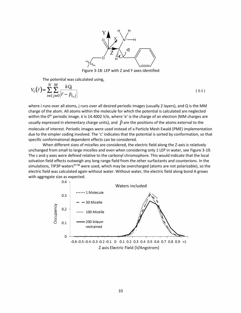
33

Figure 3-18: LEP with Z and Y axes identified

The potential was calculated using,

N

i

M

j ji

ic

pr

kQrV

1 0 ,

( 3-1 )

where i runs over all atoms, j runs over all desired periodic images (usually 2 layers), and Q is the MM charge of the atom. All atoms within the molecule for which the potential is calculated are neglected within the 0th periodic image. k is 14.4002 V/e, where ‘e’ is the charge of an electron (MM charges are

usually expressed in elementary charge units), and p

are the positions of the atoms external to the

molecule of interest. Periodic images were used instead of a Particle Mesh Ewald (PME) implementation due to the simpler coding involved. The ‘c’ indicates that the potential is sorted by conformation, so that specific conformational dependent effects can be considered.

When different sizes of micelles are considered, the electric field along the Z-axis is relatively unchanged from small to large micelles and even when considering only 1 LEP in water, see Figure 3-19. The z and y axes were defined relative to the carbonyl chromophore. This would indicate that the local solvation field effects outweigh any long range field from the other surfactants and counterions. In the simulations, TIP3P waters97-98 were used, which may be overcharged (atoms are not polarizable), so the electric field was calculated again without water. Without water, the electric field along bond A grows with aggregate size as expected.

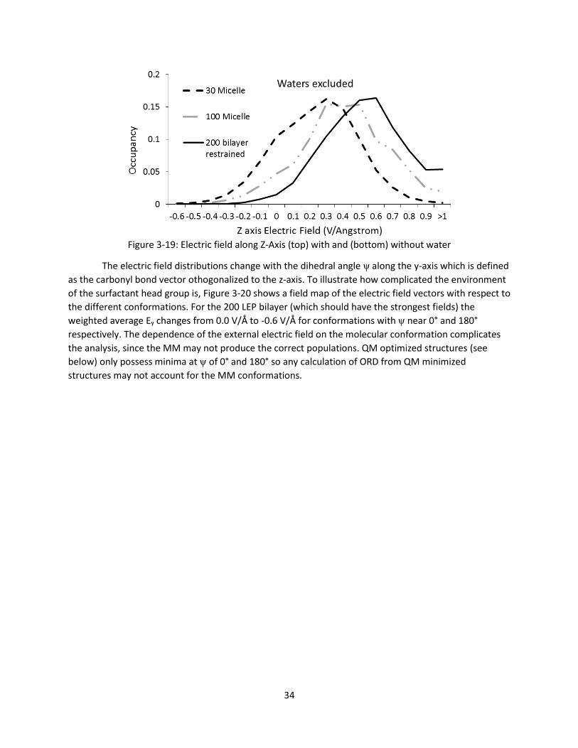
34

Figure 3-19: Electric field along Z-Axis (top) with and (bottom) without water

The electric field distributions change with the dihedral angle ψ along the y-axis which is defined

as the carbonyl bond vector othogonalized to the z-axis. To illustrate how complicated the environment

of the surfactant head group is, Figure 3-20 shows a field map of the electric field vectors with respect to

the different conformations. For the 200 LEP bilayer (which should have the strongest fields) the

weighted average Ey changes from 0.0 V/Å to -0.6 V/Å for conformations with ψ near 0° and 180°

respectively. The dependence of the external electric field on the molecular conformation complicates

the analysis, since the MM may not produce the correct populations. QM optimized structures (see

below) only possess minima at ψ of 0° and 180° so any calculation of ORD from QM minimized

structures may not account for the MM conformations.

35

Figure 3-20: Electric field along x and y Axes with water from 200 LEP bilayer simulation for specific

conformations (φ and ψ values)

Since the field along the z-axis grows when waters are excluded, ORD calculations were

performed with applied external fields with similar magnitudes on the model system EEP. The applied

field is seen to have very little effect on the SOR values, if energy differences between conformers in the

presence of electric field are not considered, see Figure 3-21. When energy changes for the different

conformers in the external field are taken into account, the Boltzmann weighting factors change in the

applied field and give a dramatic change in the averaged SOR. The change in SOR from the field may not

be from the external electric field changing the electronic structure of the surfactant molecules, but

from the preferential change in energy of some conformers.

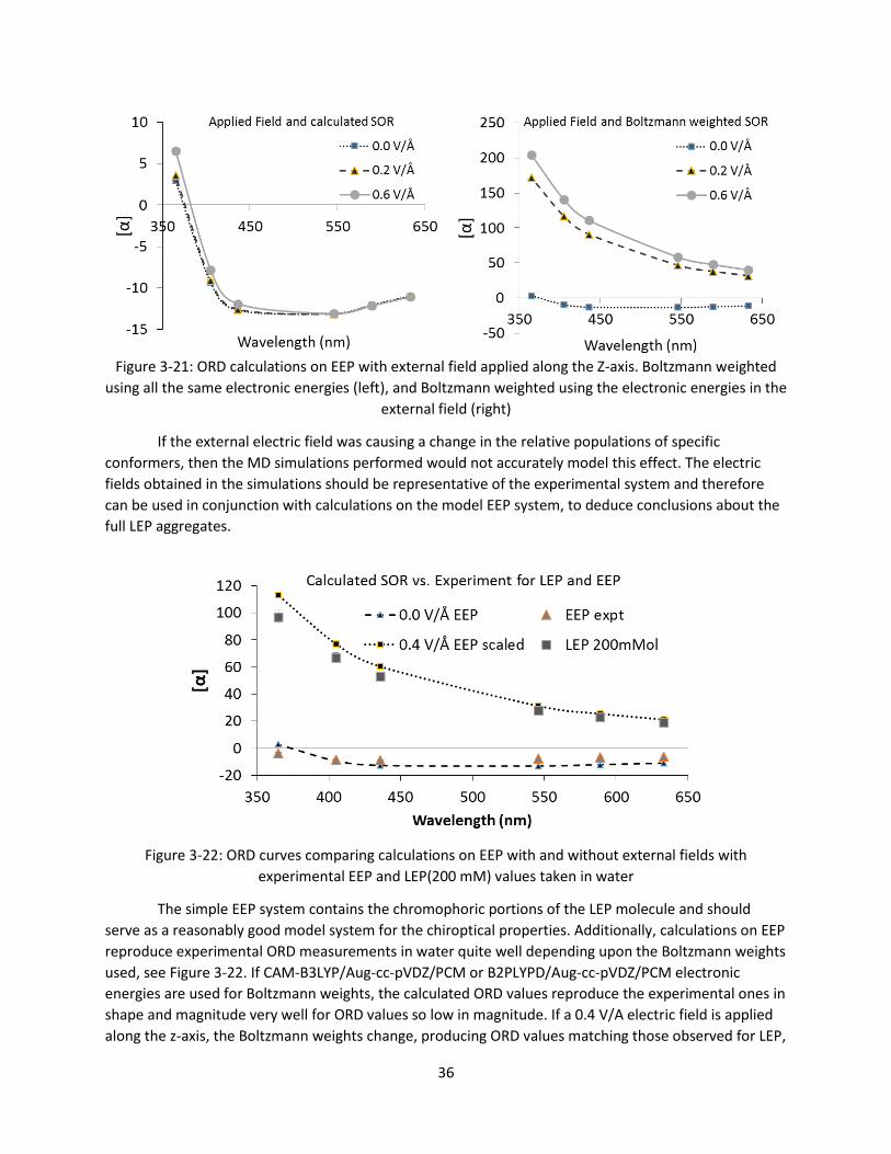
36

Figure 3-21: ORD calculations on EEP with external field applied along the Z-axis. Boltzmann weighted

using all the same electronic energies (left), and Boltzmann weighted using the electronic energies in the

external field (right)

If the external electric field was causing a change in the relative populations of specific

conformers, then the MD simulations performed would not accurately model this effect. The electric

fields obtained in the simulations should be representative of the experimental system and therefore

can be used in conjunction with calculations on the model EEP system, to deduce conclusions about the

full LEP aggregates.

Figure 3-22: ORD curves comparing calculations on EEP with and without external fields with

experimental EEP and LEP(200 mM) values taken in water

The simple EEP system contains the chromophoric portions of the LEP molecule and should

serve as a reasonably good model system for the chiroptical properties. Additionally, calculations on EEP

reproduce experimental ORD measurements in water quite well depending upon the Boltzmann weights

used, see Figure 3-22. If CAM-B3LYP/Aug-cc-pVDZ/PCM or B2PLYPD/Aug-cc-pVDZ/PCM electronic

energies are used for Boltzmann weights, the calculated ORD values reproduce the experimental ones in

shape and magnitude very well for ORD values so low in magnitude. If a 0.4 V/A electric field is applied

along the z-axis, the Boltzmann weights change, producing ORD values matching those observed for LEP,

37

when adjusted for mass difference, see Figure 3-22. This indicates that the change in SOR upon

aggregation could come from the electric field changing the populations of the surfactant

conformations, and is a combination of electrostatic environment and ensuing conformational changes

mentioned above. The effect can be thought to come from the polarizability of the surfactant molecules

in a self-created electrostatic environment, which may be difficult to model with MM force fields.

In this case however, the trend in the Boltzmann weighted conformations is the opposite to that

observed in experiment for concentrated solutions of LEP.80-81 The observed trend is that conformations

with values of φ near ±60° increase with increasing concentration. The calculated trend with increasing

field strength is for conformations with values of φ near 180° to increase with the applied field, shown in

Table 3-1 (since the calculations are done for EEP there are 3 conformations of the ethyl group/tail). The

failure of the electric field Boltzmann weights may be from the simplification in our calculations of the

complex environment into a single component of the external field, or that the optimized structures do

not include explicit solvent. It seems that a more involved calculation of the specific electric field effects

is needed.

Conformation #

Ψ (deg) φ (deg) Weight No Field

Weight 0.4 V/Å Field

1 -19 -177 0.380 0.435

2 -17 -176 0.160 0.247

3 -16 -178 0.136 0.291

4 7 -66 0.171 0.000

5 6 -68 0.044 0.000

6 6 -67 0.060 0.000

8 167 176 0.021 0.026

13 -28 67 0.027 0.000

Table 3-1: Boltzmann weights from Cam-B3LYP/Aug-cc-pVDZ/PCM calculations with and without an

applied electric field

QM/MM-MD using the PM6 Hamiltonian To correctly predict the behavior of charged surfactants in their self-created electric field, a

method is needed to calculate forces for the MD that account for external field’s perturbation on the

electronic structure and relative energies of the molecules. Polarizable force fields have been

developed, but they are based on atomic polarizabilities and may be influenced by the solvation or local

field, and may misrepresent the true nature of the solvated species, because the parameters used are

still derived from calculations without solvent.

To model the solute in the presence of solvent and other environmental factors, forces derived

from semi-empirical QM methods using the PM6 Hamiltonian were employed in the QM/MM-MD

method.42 The QM region was restricted by including only one LEP as a methyl ester (only the

headgroup to the first carbon in the 12 carbon chain capped with H) the tail portion will experience MM

forces, see Figure 3-23). The 20-25 water molecules closest to the hydrogen bonding atoms were also

included to constitute the first and part of the second solvation shells and possibly provide more

accurate conformational statistics of the solute, see Figure 3-23.

38

Figure 3-23: An Example QM region containing 1 LEP headgroup and 25 explicit water molecules

Both conformational effects and the long range electrostatic effects can be tested using the

QM/MM-MD simulations, because the exact range of charges included in the QM region can be

specified. By comparing the simulations of a micellar system with and without long range contributions

from other surfactant molecules the true effect of the electrostatics may be sorted out from the

conformational effects, see Figure 3-24. To that end, QM/MM-MD simulations were performed on the 1

and 40 LEP systems with full PME and a version of the 40 LEP system with no PME and only 5 Å of MM

charges in the QM region. Inclusion of only 5 Å of MM charges will allow the solute to experience the

local field effects of solvation, but not the long range effects from many charged molecules.

Figure 3-24: QM/MM-MD simulations with charges included over (left) infinite and (right) a limited

range

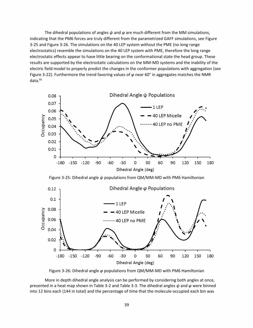
39

The dihedral populations of angles ψ and φ are much different from the MM simulations,

indicating that the PM6 forces are truly different from the parametrized GAFF simulations, see Figure

3-25 and Figure 3-26. The simulations on the 40 LEP system without the PME (no long range

electrostatics) resemble the simulations on the 40 LEP system with PME, therefore the long range

electrostatic effects appear to have little bearing on the conformational state the head group. These

results are supported by the electrostatic calculations on the MM-MD systems and the inability of the

electric field model to properly predict the changes in the conformer populations with aggregation (see

Figure 3-22). Furthermore the trend favoring values of φ near 60° in aggregates matches the NMR

data.81

Figure 3-25: Dihedral angle ψ populations from QM/MM-MD with PM6 Hamiltonian

Figure 3-26: Dihedral angle φ populations from QM/MM-MD with PM6 Hamiltonian

More in depth dihedral angle analysis can be performed by considering both angles at once, presented in a heat map shown in Table 3-2 and Table 3-3. The dihedral angles ψ and φ were binned into 12 bins each (144 in total) and the percentage of time that the molecule occupied each bin was

40

calculated. ORD at 589, 436, and 365 nm at the CAM-B3LYP/Aug-cc-pVDZ/PCM level was calculated for each bin from B3LYP/6-31G*/PCM relaxed scan structures of EEP. The calculated ORD was then weighted by the dihedral occupancy and scaled to account for the mass difference of LEP and EEP to obtain a predicted ORD, shown in Figure 3-27.

Table 3-2: Dihedral occupancies of 40 LEP Micelle with PM6 forces

Table 3-3: Dihedral occupancies of 1 LEP in water with PM6 forces

0 30 60 90 120 150 180 210 240 270 300 330

0 0.1 0.0 0.0 0.0 0.0 0.1 0.0 0.0 0.0 0.0 0.0 0.1

30 0.0 0.0 0.0 0.0 0.3 0.4 0.1 0.0 0.0 0.1 0.4 0.4

60 0.2 0.0 0.0 0.3 3.2 4.1 1.4 0.7 1.1 2.0 3.2 1.8

90 0.3 0.1 0.1 0.3 2.6 5.9 5.0 4.3 4.0 2.5 2.3 1.5

120 0.6 0.2 0.0 0.1 0.7 1.9 2.5 2.1 1.2 0.5 0.6 0.8

150 0.8 0.2 0.1 0.1 0.7 2.3 3.7 3.3 1.3 0.6 0.6 1.0

180 1.0 0.3 0.0 0.1 0.5 1.5 2.5 2.0 0.8 0.4 0.7 1.2

210 0.1 0.0 0.0 0.0 0.0 0.1 0.1 0.1 0.1 0.1 0.1 0.1

240 0.0 0.0 0.0 0.0 0.0 0.0 0.0 0.0 0.0 0.0 0.0 0.0

270 0.3 0.1 0.0 0.0 0.0 0.2 0.6 0.6 0.2 0.1 0.3 0.8

300 1.4 0.1 0.0 0.0 0.0 0.8 2.4 0.9 0.1 0.1 0.3 1.5

330 0.5 0.0 0.0 0.0 0.0 0.5 0.6 0.0 0.0 0.0 0.1 0.6

Dihedral Occpancies for 40 LEP Micelle QMMM-MD PM6

ψ

φ

0 30 60 90 120 150 180 210 240 270 300 330

0 0.1 0.0 0.0 0.0 0.0 0.1 0.0 0.0 0.0 0.0 0.1 0.3

30 0.0 0.0 0.0 0.0 0.3 0.3 0.1 0.0 0.0 0.1 0.8 0.8

60 0.4 0.1 0.0 0.2 1.3 2.1 0.8 0.4 0.5 1.3 4.5 3.2

90 0.8 0.3 0.1 0.2 0.7 2.0 1.5 1.2 0.9 1.1 2.0 2.2

120 0.8 0.3 0.1 0.1 0.2 0.8 1.0 0.7 0.4 0.3 0.6 1.1

150 2.5 0.9 0.2 0.2 0.7 2.2 2.9 2.4 1.0 0.7 1.4 2.7

180 3.9 1.3 0.3 0.3 1.0 2.4 2.8 1.9 1.3 1.0 2.1 4.4

210 0.3 0.1 0.0 0.0 0.0 0.1 0.2 0.2 0.1 0.1 0.2 0.4

240 0.0 0.0 0.0 0.0 0.0 0.0 0.0 0.0 0.0 0.0 0.0 0.0

270 0.7 0.2 0.0 0.0 0.1 0.4 0.5 0.3 0.1 0.1 0.3 0.9

300 2.7 0.5 0.0 0.0 0.1 1.7 2.7 0.7 0.1 0.0 0.4 2.8

330 1.0 0.1 0.0 0.0 0.1 1.1 0.8 0.0 0.0 0.0 0.2 1.6

Dihedral Occpancies for 1 LEP in water QMMM-MD PM6

ψ

φ

41

Calculation of the SOR from the observed dihedral populations as opposed to snapshots from

the trajectory allows for much faster calculation of the desired property (144 ORD calculations vs +500)

with much better convergence in the average.

Figure 3-27: ORD calculated from QM/MM-MD conformational populations

Although the trend of increasing SOR is reproduced with the PM6 Hamiltonian, ECD calculations using the same dihedral populations do not match the experimental trend, shown in Figure 3-28. There is some apparent change in the 220 nm region, however the trend is out of order with order with experiment which shows increasing positive ECD with increasing concentration (see Figure 3-9). The discrepancy could come from the accuracy of the conformational statistics produced by the semi-empirical PM6 method, or from some other effect not considered in the ECD calculations such as self-generated electric fields or specific hydrogen bonding interactions.

Figure 3-28: ECD calculated using populations found from QM/MM-MD at the

CAM-B3LYP/Aug-cc-pVDZ/PCM level

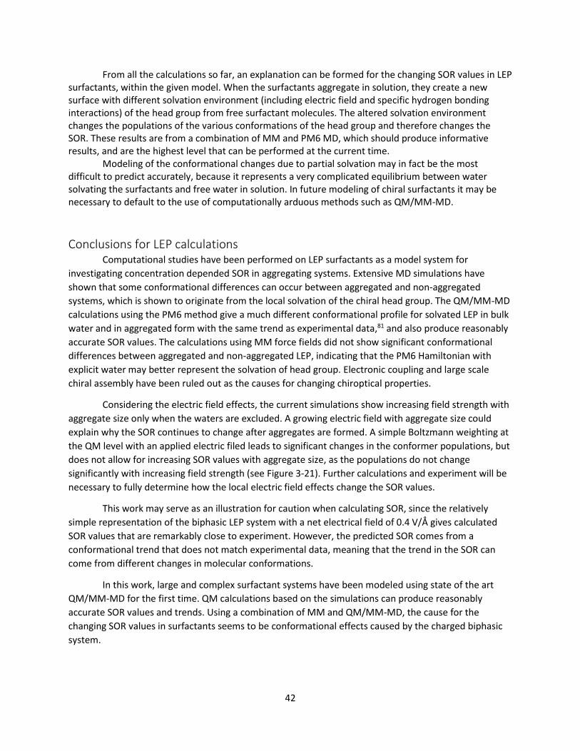
42

From all the calculations so far, an explanation can be formed for the changing SOR values in LEP surfactants, within the given model. When the surfactants aggregate in solution, they create a new surface with different solvation environment (including electric field and specific hydrogen bonding interactions) of the head group from free surfactant molecules. The altered solvation environment changes the populations of the various conformations of the head group and therefore changes the SOR. These results are from a combination of MM and PM6 MD, which should produce informative results, and are the highest level that can be performed at the current time. Modeling of the conformational changes due to partial solvation may in fact be the most difficult to predict accurately, because it represents a very complicated equilibrium between water solvating the surfactants and free water in solution. In future modeling of chiral surfactants it may be necessary to default to the use of computationally arduous methods such as QM/MM-MD.

Conclusions for LEP calculations Computational studies have been performed on LEP surfactants as a model system for

investigating concentration depended SOR in aggregating systems. Extensive MD simulations have

shown that some conformational differences can occur between aggregated and non-aggregated

systems, which is shown to originate from the local solvation of the chiral head group. The QM/MM-MD

calculations using the PM6 method give a much different conformational profile for solvated LEP in bulk

water and in aggregated form with the same trend as experimental data,81 and also produce reasonably

accurate SOR values. The calculations using MM force fields did not show significant conformational

differences between aggregated and non-aggregated LEP, indicating that the PM6 Hamiltonian with

explicit water may better represent the solvation of head group. Electronic coupling and large scale

chiral assembly have been ruled out as the causes for changing chiroptical properties.

Considering the electric field effects, the current simulations show increasing field strength with

aggregate size only when the waters are excluded. A growing electric field with aggregate size could

explain why the SOR continues to change after aggregates are formed. A simple Boltzmann weighting at

the QM level with an applied electric filed leads to significant changes in the conformer populations, but

does not allow for increasing SOR values with aggregate size, as the populations do not change

significantly with increasing field strength (see Figure 3-21). Further calculations and experiment will be

necessary to fully determine how the local electric field effects change the SOR values.

This work may serve as an illustration for caution when calculating SOR, since the relatively

simple representation of the biphasic LEP system with a net electrical field of 0.4 V/Å gives calculated

SOR values that are remarkably close to experiment. However, the predicted SOR comes from a

conformational trend that does not match experimental data, meaning that the trend in the SOR can

come from different changes in molecular conformations.

In this work, large and complex surfactant systems have been modeled using state of the art

QM/MM-MD for the first time. QM calculations based on the simulations can produce reasonably

accurate SOR values and trends. Using a combination of MM and QM/MM-MD, the cause for the

changing SOR values in surfactants seems to be conformational effects caused by the charged biphasic

system.

43

Details on the MD simulations The MM-MD simulations on LEP were performed in Amber12 using the GAFFlipid force field,

with some of the important dihedrals fitted to QM energies.96, 99 Restrained Electrostatic Potential Derived Charges were obtained from the online server R.E.D.-III using the standard method, and were used in all LEP MD simulations.100 The following procedures were used in the MD simulation on LEP micelles: structures for various micellar aggregation numbers were created using the software Packmol.95 Restraints were placed on the positions of the head and tail atoms to create a starting structure with straight tails and all head groups towards the outside. To the starting surfactant structure, chloride ions were added at favorable positions to produce a net system charge of zero using the program tleap.101 The micellar system was then surrounded by pre-equilibrated TIP3P water molecules, in a truncated octahedron box or rectangular box using tleap. Then enough waters were added to provide a 15-20 Å layer of water between the surfactant molecules and the periodic boundaries. The fully solvated systems were then run through a minimization and equilibration procedure used for lipid bilayers.96 First a minimization with position restraints on surfactants (250 steps steepest descent then 750 steps conjugate gradient). Second a minimization without position restraints on surfactants (2500 steps steepest descent then 2500 steps conjugate gradient). Then a temperature equilibration to 300 K (thermostat using Langevin dynamics with collision frequency of 1.0 ps-1) with position restraints on surfactants for 20 ps. Then a 50 ps pressure equilibration is performed without position restraints using anisotropic Berendsen pressure control to 1 bar with a time constant 0.5 ps. Finally a 170 ps to 1 ns trial simulation is performed, after which the energy, temperature, pressure, and density are checked for stability. Extended MD was then run for 100-1000 ns depending upon the system in the GPU accelerated version of Amber12.101 Long range electrostatics was handled by Particle Mesh Ewald (PME) summation. Hydrogens were confined with the SHAKE algorithm102 allowing for an integration timestep of 2 fs, which was used for all MD unless otherwise noted. Micellar structures larger than 40 LEP units were not stable with the GAFFlipid parameters and TIP3P waters, and tended to dissociate. The 200 LEP bilayer required weak position restraints in the tail to remain in bilayer form. QM/MM-MD simulations at the PM6 level were performed using the AmberTools2015 sander

module,103 with custom code to allow for multiple solvent bonding sites. Hydrogens were confined with

the SHAKE algorithm which allowed for a timestep of 2 fs. Starting structures for QM/MM-MD were

taken from MM-MD simulations equilibrated with the default method. 15-24 replicates were started

from different points in a MM-MD simulation and run separately to improve the sampling, and the first

20 ps of the replicate trajectories were not used for the analysis. For the 40 LEP simulations, a different

LEP molecule was chosen to represent the QM region for each replicate. The replicates were combined

in the end to produce total simulation lengths of: 61.6 ns for 1 LEP, 68.3 ns for 40 LEP with PME, and

108.5 ns for 40 LEP without PME. For simulations with 1 and 40 LEP molecules, 25 and 20 water

molecules were included in the QM region respectively, enough to extend the QM region into the

second solvation shell.

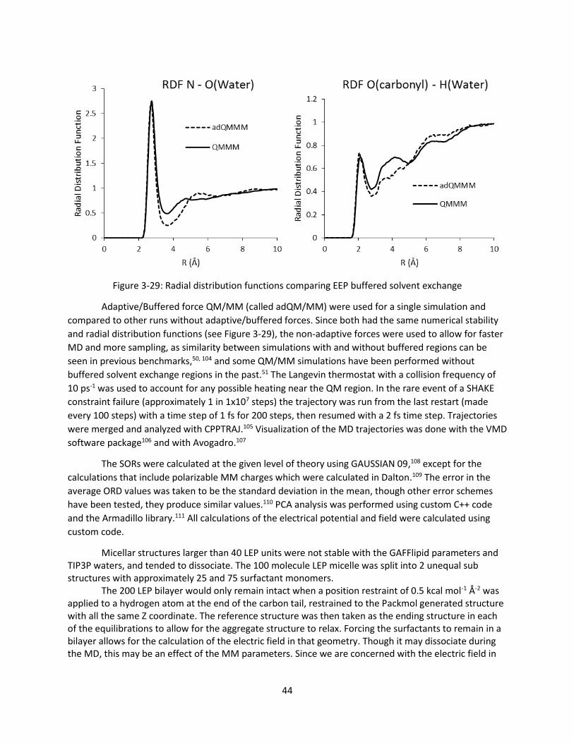
44

Figure 3-29: Radial distribution functions comparing EEP buffered solvent exchange

Adaptive/Buffered force QM/MM (called adQM/MM) were used for a single simulation and

compared to other runs without adaptive/buffered forces. Since both had the same numerical stability

and radial distribution functions (see Figure 3-29), the non-adaptive forces were used to allow for faster

MD and more sampling, as similarity between simulations with and without buffered regions can be

seen in previous benchmarks,50, 104 and some QM/MM simulations have been performed without

buffered solvent exchange regions in the past.51 The Langevin thermostat with a collision frequency of

10 ps-1 was used to account for any possible heating near the QM region. In the rare event of a SHAKE

constraint failure (approximately 1 in 1x107 steps) the trajectory was run from the last restart (made

every 100 steps) with a time step of 1 fs for 200 steps, then resumed with a 2 fs time step. Trajectories

were merged and analyzed with CPPTRAJ.105 Visualization of the MD trajectories was done with the VMD

software package106 and with Avogadro.107

The SORs were calculated at the given level of theory using GAUSSIAN 09,108 except for the

calculations that include polarizable MM charges which were calculated in Dalton.109 The error in the

average ORD values was taken to be the standard deviation in the mean, though other error schemes

have been tested, they produce similar values.110 PCA analysis was performed using custom C++ code

and the Armadillo library.111 All calculations of the electrical potential and field were calculated using

custom code.

Micellar structures larger than 40 LEP units were not stable with the GAFFlipid parameters and TIP3P waters, and tended to dissociate. The 100 molecule LEP micelle was split into 2 unequal sub structures with approximately 25 and 75 surfactant monomers.

The 200 LEP bilayer would only remain intact when a position restraint of 0.5 kcal mol-1 Å-2 was applied to a hydrogen atom at the end of the carbon tail, restrained to the Packmol generated structure with all the same Z coordinate. The reference structure was then taken as the ending structure in each of the equilibrations to allow for the aggregate structure to relax. Forcing the surfactants to remain in a bilayer allows for the calculation of the electric field in that geometry. Though it may dissociate during the MD, this may be an effect of the MM parameters. Since we are concerned with the electric field in

45

these studies, forcing the aggregates into a particular structure, could be a way to study how the geometry of the aggregate effects the chiroptical properties. The number of waters included in the simulations, box shape, simulation time, and the trajectories use are shown in Table 3-4.

Table 3-4: LEP simulation details

Experimental Methods LEP was synthesized as described previously,80 except for the relative amounts of reagents used.

First, 0.75 ml of thionyl chloride was added slowly to a rapidly stirring mixture of 10 ml of cold dodecanol. After 15 min, 1 g of L-phenylalanine was added to the reaction mixture was slowly heated to 70 °C for 6 hr. The reaction mixture was then allowed to cool until 30 ml of ethyl acetate could be added safely. This was then run through a procedure of centrifugation, cooling (-80 °C), centrifugation, and removal of liquid layer, and filtration three times in ethyl acetate before it was precipitated in diethyl ether to yield a white solid in 60 % overall yield. The products purity was confirmed by NMR. EEP was obtained from Sigma Aldrich. All regents were purchased from Sigma Aldrich. OR was measured at six different wavelengths, namely, 633, 589, 546, 436 405, and 365 nm in deionized water using an Autopol IV polarimeter in a 0.5 or 2 dm temperature controlled cell. ECD measurements were made in either a 0.01, 0.1, 1.0, or 5.0 cm quartz cell or an adjustable pathlength (10-2000 micron) BaF2 cell with a Jasco J-720 spectrometer.

# LEP 1 15 30 40 100 200

Structure -- Micelle Micelle Micelle Micelle Bilayer

# Water 5515 9509 9261 29574 6917 4000

Box Shape Trunc. Oct. Rectangular Rectangular Trunc. Oct. Rectangular Rectangular

Simulation

length500 ns 200 ns 100 ns 100 ns 100 ns 8 ns

UsageElectric Field,

ORD CalculationElectric Field Electric Field ORD Calculation Electric Field Electric Field

LEP GAFFLipid Simulation Details

46

Chapter 4 The Dissymmetry Factor spectrum: A novel chiroptical

spectral analysis method

The work from this chapter can be found in The Journal of Physical Chemistry A article112 “Similarity in

dissymmetry factor spectra: a quantitative measure of comparison between experimental and predicted

vibrational circular dichroism” and the Chirality article55 “Comparison of experimental and calculated

chiroptical spectra for chiral molecular structure determination”.

Introduction An unprecedented growth in the applications of chiroptical spectroscopy for molecular structure

determination has occurred in recent years, due to the availability of computational resources with faster processor speeds for quantum chemical spectral predictions and of dedicated instrumentation for experimental spectral measurements. However, what happens when the systems studied are not always well modeled by the QC methods available? Or what if some parts of the calculated spectrum suggest one configuration, while other regions suggest a different configuration?113 To handle situations like these, the concept of robustness was developed by Nicu and Baerends.114

A robust, calculated VCD band is not likely to change sign when the computational parameters are changed; this includes minor perturbations of the structure. The concept lies in the rotational strength of a transition being the product of electric dipole and magnetic dipole transition moments, given as,18

kimikemek ikkiR ,,ImIm μμμμ ( 4-1 )

where 𝝁𝑒 and 𝝁𝑚 are, respectively, the electric and magnetic dipole moment operators. For the vibrational transitions under consideration here, |𝑖⟩ and |𝑘⟩ represent the ground and excited vibrational states, both belonging to the same ground electronic state. The corresponding VA is determined by the dipole strength Dk, given as

2

,

2

ikeeeek kiikkiD μμμμ ( 4-2 )

Reliability in the predictions of Rk is crucial for making accurate predictions of absolute configurations.

As the scalar product of electric and magnetic dipole transition moment vectors, ike,μ and kim,μ ,

rotational strength is written as,114

ξcos,, kimikekR ( 4-3 )

where ξ is the angle between the two vectors. When ξ is close to 90°, the sign of 𝑅𝑘 can change with only a minimal perturbation of geometry or computational parameters. In light of this issue, the concept of band robustness has been introduced by Nicu and Baerends using the angle ξ between transition moment vectors.114. However Gobi and Magyarfalvi pointed out that the angle ξ is an origin dependent quantity and proposed a criterion for band robustness using,115

47

k

k

ike

kimk

D

R

,

, cos

ξζ ( 4-4 )

where 𝜁𝑘, is a unitless number in the range of 10-3 to 10-5, and for convenience expressed as parts per million (ppm). Gobi and Magyarfalvi suggested that the fundamental vibrational transitions with calculated 𝜁𝑘 values above 10 ppm could be considered robust and used in the determination of absolute configuration, while those under 10 ppm should not be considered.115

Gobi and Magyarfalvi’s robustness criterion is convenient when there are a few well separated bands, but often the transitions will overlap and the experimental quantities R and D are not readily found. To get around this problem, we adapted Kuhn’s Dissymmetry Factor (DF) for kth band, defined116-

117

k

k

k

k

k

kk

D

R

A

Ag

4

( 4-5 )

Into the form of the DF spectrum, defined as,

x

x

xA

xAxg

( 4-6 )

where x is the running x-axis index representing wavenumber, , or wavelength, λ. The dissymmetry factor of individual bands applies to integrated band intensities while dissymmetry factor spectrum applies to the entire spectral region of interest. The advantage of the DF spectrum is that the individual experimental 𝑅𝑘’s and 𝐷𝑘’s need not be determined. The DF spectrum can be derived from original absorbance and CD spectra. A theoretical analog can similarly be made from simulated absorbance and CD spectra for comparison to experiment. Furthermore the DF spectral comparison can be used for VCD, ECD, and ROA methods. For vibrational spectroscopy the DF spectrum is called the Vibrational Dissymmetry Factor (VDF) spectrum and for spectra in the UV and visible regions it is referred to as the Electronic Dissymmetry Factor (EDF) spectrum. For ROA, the analog of the DF spectrum is the dimensionless circular intensity difference (CID) and is defined as55, 116

k

k

S

P

II

II

( 4-7 )

Where the numerator is determined by Pk, the Raman circular intensity difference activity and the denominator is determined by Sk, the Raman activity. I is the intensity of scattered light, with subscript α and β represent right handed and left handed polarization of the scattered light and the superscripts γ and δ represent right handed and left handed polarization of the incident light.

Method We originally hypothesized that the DF spectrum should be an additional observable quantity. DF

spectra should also possess a number of advantageous properties that allow for better comparison

between theory and experiment. The following properties come from the definition of the DF:

48

1) The concept of robustness can be applied easily to DF spectra by introducing a threshold value,

TE, that cuts off all non-robust values. The robustness criterion we use is determined by the

experimental limits of measurability (well over noise) of 40 ppm for VCD and ROA spectra, but

can be varied for individual experimental measurements.

2) The x-axis scale factor that maximizes similarity may be different for absorbance, CD, and DF

spectra.

3) By comparing the DF spectra between theory and experiment, both absorption and CD are

taken into account.

4) DF spectra are independent of concentration and sample thickness/path length. As a

consequence, any errors in the experimental concentrations and path lengths are canceled out

in experimental DF spectra.

5) DF spectra reweight the bands from CD spectra and therefore may look entirely different from

the original data. This new comparison function can improve the confidence or cast doubt on

the agreement with CD spectra.

6) In molecules with many conformations, the DF will be diminished in regions with differing CD

between conformations.

To test this hypothesis, we must compare calculated and experimental DF spectra for many different

molecules.

Certain considerations must be made for the DF spectrum. Noise is always present (especially in CD spectroscopy) and in regions of low absorption, the DF behaves abnormally because it amplifies the noise to very large values. To fix this problem, an absorbance threshold (τA) for each experimental absorbance spectrum was introduced. If absorbance falls below this cutoff, then the DF is defined to be zero. The DF can be fully defined as,

Otherwise

xandTx

xif

x

x

xg

AC

,

,

0

( 4-8 )

Where τA is the absorbance threshold and TC is the minimum robustness value. The DF spectrum is calculated at each point for which Δε and ε are reliable (above the noise levels).

Results

Initial tests of the VDF To test the concept of the VDF spectrum, we began with six small compounds with known

absolute configurations, few conformations, and strong VCD signals, shown in Figure 4-1. Calculations on the test molecules come from various sources summarized in Table 4-1.118-121

49

Figure 4-1: Initial compounds considered in the VDF study

Name Solvent Low Energy Conformers

Functional/Basis Source

(R)-(+)-3-chloro-1-butyne CCl4 1 B3LYP/Aug-cc-pVTZ He et al.

(1S)-(-)-pinene Neat 1 B3LYP/Aug-cc-pVDZ Calculated*

(3R)-(+)-methylcyclopentanone CCl4 2 B3LYP/Aug-cc-pVTZ He et al.

(3R)-(+)-methylcyclohexanone CCl4 2 B3LYP/Aug-cc-pVDZ Calculated*

(1R)-(+)-camphor CCl4 1 B3PW91/TZVP Longhi et al.

(S)-(+)-epichlorohydrin CCl4 3 B3LYP/6-31G* Wang and Polavarapu.

Table 4-1: Details for the six VDF test compounds. *Calculated for the study118-121

The case of (3R)-(+)-methylcyclopentanone is very informative and a good example for the use of DF spectral analysis. The VA and VCD spectra have a large transition at approximately 1150 cm-1 that is misaligned with respect to other transitions, see Figure 4-2 and Figure 4-3. When the ratio is taken, the bands that have primarily electric dipole transition moments are diminished and accordingly the VDF around 1150 cm-1 is much smaller than the other bands, shown in Figure 4-4. The bands that have large VDF should have higher signal-to-noise ratio and be the most sensitive to the chirality and be the best to compare between theory and experiment. Similarity analysis shows the improved agreement at a wavenumber scale factor of 0.98, see Figure 4-5, which is closer to what is expected for frequencies calculated using the B3LYP functional.

50

Figure 4-2: The calculated and experimental VA spectra of (3R)-(+)-methylcyclopentanone

Figure 4-3: The calculated and experimental VCD spectra of (3R)-(+)-methylcyclopentanone

51

Figure 4-4: The calculated and experimental VDF spectra of (3R)-(+)-methylcyclopentanone. τA was taken

to be 2.4 L mol-1 cm-1

Figure 4-5: Vibrational similarity analysis of (3R)-(+)-methylcyclopentanone

In the case of (3R)-(+)-methylcyclopentanone, the VDF had better agreement between

experiment and theory than the corresponding VCD, which was also observed in two other cases, see

Table 4-2.

52

Molecule Max SimVA

Max SimVCD

Max SimVDF

(R)-(+)-3-chloro-1-butyne 0.71 0.50 0.70 (1S)-(-)-α-pinene 0.90 0.84 0.86

(3R)-(+)-methylcyclopentanone 0.74 0.48 0.53 (3R)-(+)-methylcyclohexanone 0.76 0.84 0.76

(1R)-(+)-camphor 0.68 0.60 0.56 (S)-(+)-epichlorohydrin 0.83 0.64 0.49

Table 4-2: Maximum similarity ratings for the six VDF test cases

Generalization to ECD and ROA The similarity between the vibrational and electronic methods led us to generalize the DF

spectral analysis methods to ECD and ROA techniques. The same principles are used in all three types of

chiroptical spectroscopy, so the use of DF method should also be advantageous in ECD and ROA analysis.

The same procedure used in generation of the VDF can be applied to generate the EDF, but the CID

calculated with the relation

Otherwise

IIandTII

II

ifII

II

RC

,

,

0

( 4-9 )

The differences between the three methods are how the transitions are calculated, how the spectra are

simulated, the instrumentation used, and how the observables are defined. These differences are rather

technical and distract from the focus of this section, but the differences do not change the DF method.

Therefore these detail will not be presented here, but can be found in Chirality.55

The test calculation of the EDF was performed on (aR)-(+)-3,3'-diphenyl-[2,2'-binaphthalene]-

1,1'-diol, often referred to as Vanol, see Figure 4-6.122 The experimental EA and ECD spectra collected in

acetonitrile are shown with the calculated spectra at the CAM-B3LYP/6-311++G(2d,2p)/PCM level in

Figure 4-7 and Figure 4-8. The corresponding EDF spectrum is shown in Figure 4-9.

53

Figure 4-6: (aR)-(+)-3,3'-diphenyl-[2,2'-binaphthalene]-1,1'-diol, also called Vanol

Figure 4-7: The EA of (aR)-(+)-Vanol in acetonitrile

Figure 4-8: The ECD of (aR)-(+)-Vanol in acetonitrile

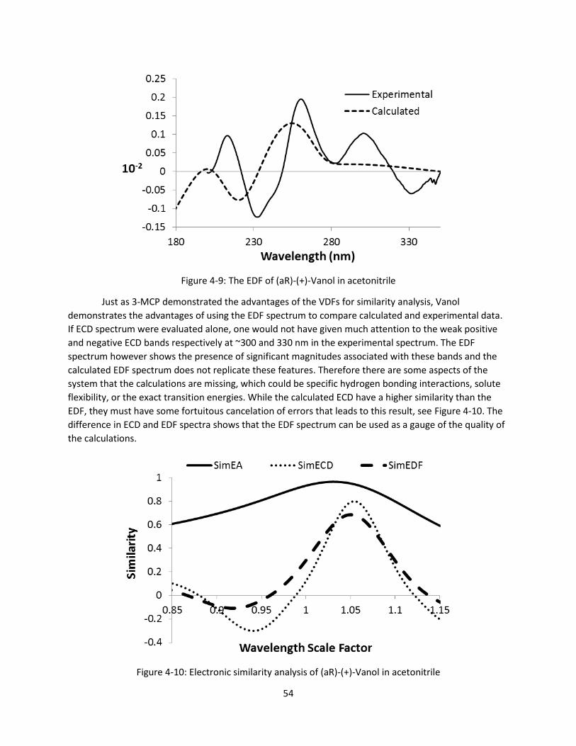
54

Figure 4-9: The EDF of (aR)-(+)-Vanol in acetonitrile

Just as 3-MCP demonstrated the advantages of the VDFs for similarity analysis, Vanol

demonstrates the advantages of using the EDF spectrum to compare calculated and experimental data.

If ECD spectrum were evaluated alone, one would not have given much attention to the weak positive

and negative ECD bands respectively at ~300 and 330 nm in the experimental spectrum. The EDF

spectrum however shows the presence of significant magnitudes associated with these bands and the

calculated EDF spectrum does not replicate these features. Therefore there are some aspects of the

system that the calculations are missing, which could be specific hydrogen bonding interactions, solute

flexibility, or the exact transition energies. While the calculated ECD have a higher similarity than the

EDF, they must have some fortuitous cancelation of errors that leads to this result, see Figure 4-10. The

difference in ECD and EDF spectra shows that the EDF spectrum can be used as a gauge of the quality of

the calculations.

Figure 4-10: Electronic similarity analysis of (aR)-(+)-Vanol in acetonitrile

55

The procedure for analysis of CID spectra is same as that for VDF spectra except that a much

wider frequency region is accessible in Raman/ROA spectroscopy. ROA instruments can routinely

measure from 200 cm-1 to 2000 cm-1, where VCD is usually limited to 800 cm-1 to 2000 cm-1.

Experimental Raman and ROA spectra are recorded in terms of photon counts; the experimental

spectral intensity axes can be scaled by an arbitrary constant to make them comparable to those of

calculated spectra, and so all Raman/ROA spectra will be presented with arbitrary scaling. Raman

spectra can have some background scattering (fluorescence) which must be removed in order to

accurately generate the CID.

The CID analysis was performed on (1S)-(-)-α-pinene since it is a common standard for ROA

spectrometers with strong ROA signals. The Raman and ROA spectra of (1S)-(-)-α-pinene are shown in

Figure 4-11 and Figure 4-12. The corresponding CID spectrum is unitless, like all DF spectra, but does not

in principle need to be scaled by to compare the calculated and experimental spectra, shown in Figure

4-13. However there may be some differences in the calculated and experimental CID intensities that

come from background fluorescence or deficiencies in the calculations. The similarity plot for (1S)-(-)-α-

pinene is shown in Figure 4-14. Since ROA spectra can be measured over a larger frequency range than

VCD/ECD spectra, there are more points of comparison between the calculated and experimental

spectra. Therefore it is less likely to see higher similarity measures for ROA/CID spectra than those for

VCD/VDF or ECD/EDF spectra.

Figure 4-11: Raman spectrum of (1S)-(-)-α-pinene as neat liquid

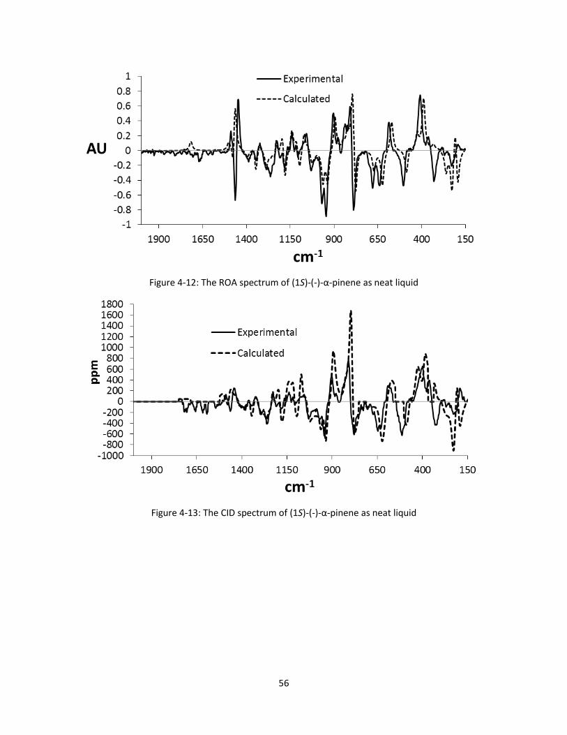
56

Figure 4-12: The ROA spectrum of (1S)-(-)-α-pinene as neat liquid

Figure 4-13: The CID spectrum of (1S)-(-)-α-pinene as neat liquid

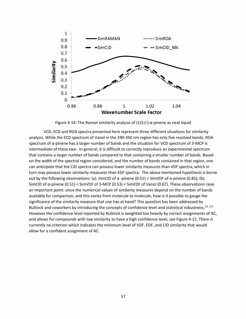
57

Figure 4-14: The Raman similarity analysis of (1S)-(-)-α-pinene as neat liquid

VCD, ECD and ROA spectra presented here represent three different situations for similarity

analysis. While the ECD spectrum of Vanol in the 190-350 nm region has only five resolved bands, ROA

spectrum of α-pinene has a larger number of bands and the situation for VCD spectrum of 3-MCP is

intermediate of these two. In general, it is difficult to correctly reproduce an experimental spectrum

that contains a larger number of bands compared to that containing a smaller number of bands. Based

on the width of the spectral region considered, and the number of bands contained in that region, one

can anticipate that the CID spectra can possess lower similarity measures than VDF spectra, which in

turn may possess lower similarity measures than EDF spectra. The above mentioned hypothesis is borne

out by the following observations: (a). SimCID of α -pinene (0.51) < SimVDF of α-pinene (0.85); (b).

SimCID of α-pinene (0.51) < SimVDF of 3-MCP (0.53) < SimEDF of Vanol (0.67). These observations raise

an important point: since the numerical values of similarity measures depend on the number of bands

available for comparison, and this varies from molecule to molecule, how is it possible to gauge the

significance of the similarity measure that one has at hand? This question has been addressed by

Bultinck and coworkers by introducing the concepts of confidence level and statistical robustness.53, 123

However the confidence level reported by Bultinck is weighted too heavily by correct assignments of AC,

and allows for compounds with low similarity to have a high confidence level, see Figure 4-15. There is

currently no criterion which indicates the minimum level of VDF, EDF, and CID similarity that would

allow for a confident assignment of AC.

58

Figure 4-15: Bultinck’s confidence level data with the confidence at various points shown53

Solvent Dependent EDF Spectrum of Binaphthol and Dibromobinaphthol During the testing stages of the EDF spectrum, [1,1′-Binaphthalene]-2,2′-diol (BN) and 6,6′-

dibromo-[1,1′-binaphthalene]-2,2′-diol (DBBN) were selected as trial compounds, shown in Figure 4-16. Due to disparities in the calculated spectral intensities the spectra were measured in 4 different solvent systems to determine if hydrogen bonding interactions with the solvent were the cause. Surprisingly, the EA and the ECD of BN changed very little between solvents, but the EDF showed a distinct solvent dependence. The EA and ECD spectra for (‒)-(aS)-BN are shown in Figure 4-17 and Figure 4-18, and the corresponding EDF with solvent dependence is shown in Figure 4-19.

Figure 4-16: The structures of BN and DBBN

59

Figure 4-17: The EA of (‒)-(aS)-BN in multiple solvents

Figure 4-18: The ECD of (‒)-(aS)-BN in multiple solvents

60

Figure 4-19: The EDF of (‒)-(aS)-BN in multiple solvents

Since the EA and ECD spectral bands have similar shapes in different solvents, the intriguing

observations are: (a). positive EDF peaks emerge where there are no apparent absorption peaks in the

experimental spectra. (b). the experimental trend for positive EDF magnitude at 245 nm seems to follow

the polarity/hydrogen bonding strength (methanol > acetonitrile > methylene chloride > cyclohexane) of

the solvent. Though BN is known to form dimers with a dimerization equilibrium constant of 1.3 ± 0.5 in

chloroform,59 the solutions used here are much too dilute (0.0013 M) to have significant population of

the dimer in the non-polar solvents. To verify that the effect of possible dimer formation is not the

source, the measurements were performed at a higher concentration in cyclohexane (0.0026 M) and no

significant change was seen in the EDF spectrum.

When the calculated EDF spectra representing the gas phase are compared with those

representing solute-acetonitrile complexes/PCM, some differences in the EDF can be seen, as shown in

Figure 4-20. The trend observed from the calculations for the EDF at ~240 nm is a slight increase in its

intensity in the gas phase calculations (representative of non-polar solvents) over that for acetonitrile

complexes/PCM. Clearly this calculated trend is at odds with the experimental observations. The current

calculations do not include aspects of vibrational substructure or the dynamic solvent-solute

interactions. It is also possible that more accurate transition energies are needed than the CAM-B3LYP

functional is providing. Moreover, because of possible hydrogen bonding interactions with acetonitrile

solvent, reproducing the experimental EDF variations from cyclohexane to acetonitrile solvent may

provide a challenge for modern quantum chemical predictions.

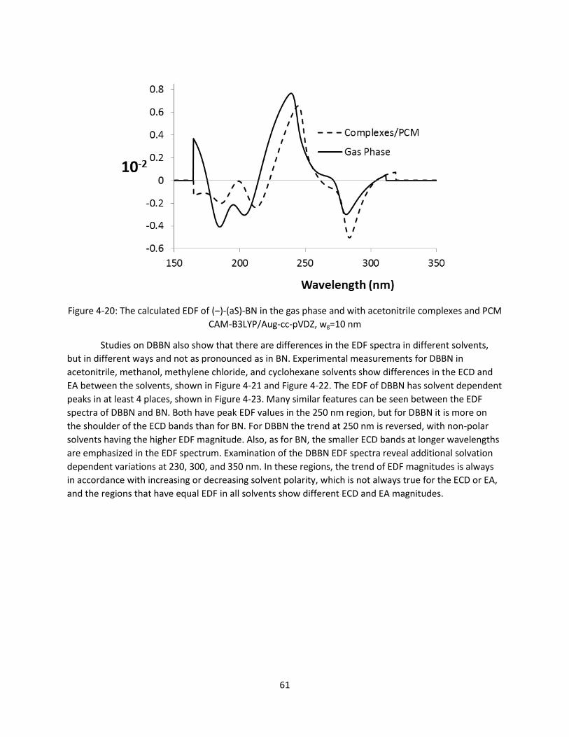
61

Figure 4-20: The calculated EDF of (‒)-(aS)-BN in the gas phase and with acetonitrile complexes and PCM

CAM-B3LYP/Aug-cc-pVDZ, wg=10 nm

Studies on DBBN also show that there are differences in the EDF spectra in different solvents,

but in different ways and not as pronounced as in BN. Experimental measurements for DBBN in

acetonitrile, methanol, methylene chloride, and cyclohexane solvents show differences in the ECD and

EA between the solvents, shown in Figure 4-21 and Figure 4-22. The EDF of DBBN has solvent dependent

peaks in at least 4 places, shown in Figure 4-23. Many similar features can be seen between the EDF

spectra of DBBN and BN. Both have peak EDF values in the 250 nm region, but for DBBN it is more on

the shoulder of the ECD bands than for BN. For DBBN the trend at 250 nm is reversed, with non-polar

solvents having the higher EDF magnitude. Also, as for BN, the smaller ECD bands at longer wavelengths

are emphasized in the EDF spectrum. Examination of the DBBN EDF spectra reveal additional solvation

dependent variations at 230, 300, and 350 nm. In these regions, the trend of EDF magnitudes is always

in accordance with increasing or decreasing solvent polarity, which is not always true for the ECD or EA,

and the regions that have equal EDF in all solvents show different ECD and EA magnitudes.

62

Figure 4-21: The EA of (+)-(aS)-DBBN in multiple solvents

Figure 4-22: The ECD of (+)-(aS)-DBBN in multiple solvents

63

Figure 4-23: The EDF of (+)-(aS)-DBBN in multiple solvents

QC calculations have been performed on DBBN in the gas phase and using optimized solvent

complexes with acetonitrile and PCM and are shown in Figure 4-24. The calculated EDF trends in DBBN

with different solvation models are similar to those observed in BN, except for DBBN they actually

match some trends in the experimental solvent dependent EDF spectra. The peaks at 240 and 220 nm

are seen to have higher EDF magnitudes in less polar solvents, and that is what is observed in the

experiment. However the calculations indicate that the EDF peaks at longer wavelengths should change

substantially, when they do not. Therefore it is likely that the solvation dependence in the EDF is from

some factor(s) not accounted for in the current TD-DFT calculations.

64

Figure 4-24: The calculated EDF of (+)-(aS)-DBBN in the gas phase and with acetonitrile complexes and

PCM, CAM-B3LYP/6-311++G(2d,2p), wg=10 nm

The prevailing practice in the literature is to analyze the ECD spectra alone. It is possible that the

experimental EDF features seen for BN and DBBN may appear in the EDF spectra of many other chiral

molecules. Unfortunately however, we could be missing all that information due to the current

unawareness of the potential associated with the EDF spectral analyses.

Robustness Reconsidered Comparisons based using the DF spectra are different from those based on transition moments.

For vibrational transitions, the electric dipole transition moments can change dramatically with solvent

conditions. However, the chirality of the vibrations may be unchanged by solvent interactions, as

evidenced by studies on a chiral sulfonic acid named CSA2, shown in Figure 4-25. CSA2 was studied as

part of a collaboration with Professor Daniel Armstrong, University of Texas at Arlington. Determination

of the AC of CSA2 was not possible due to solvent interactions (and possible dimer formation with

Barium counterions), but there were some very interesting observations from the VCD and VDF spectra.

Figure 4-25: The structure of CSA2, a chiral sulfonic acid studied in collaboration with Professor Daniel

Armstrong, University of Texas at Arlington

65

Figure 4-26: The VA spectra of CSA2 in methanol and DMSO

Figure 4-27: The VCD spectra of CSA2 in methanol and DMSO

The VA and VCD spectra for CSA2 taken in methanol and DMSO are shown in Figure 4-26 and

Figure 4-27. The VA spectra are quite different between the two solvents, most notably a strong

absorption band appearing at ~1540 cm-1 in DMSO that may be shifted to ~1430 cm-1 in methanol. The

VA spectrum in DMSO also has a strong absorption at 1250 that does not appear in the observable

region of the methanol spectrum. The VCD spectra have some similarities in the 1400 cm-1 region,

though a negative peak at 1285 cm-1 appears 4 times larger in DMSO than in methanol. It would seem

from the VA and VCD spectra that the solute molecule is greatly perturbed by the solvent. When the

VDF spectrum is considered, the two different solvent interactions produce similar spectra, shown in

Figure 4-28.

66

Figure 4-28: The VDF spectra of CSA2 in methanol and DMSO

The similarity of the VDF spectra of CSA2 in methanol and DMSO is quite astonishing considering

the differences in the VA and the VCD. The cause for this could come from the following: 1) CSA2 is a

rigid molecule. It only has one conformation, meaning there can be no changing populations of

conformers between the solvents. 2) The VA and VCD spectra come from transition dipole moments, or

how much electrons move and/or circulate. The VDF is a description of chirality and may not change

significantly with external perturbation. There is not much more that can be said about CSA2 since the

calculated VCD/VDF spectra (not shown) do not resemble the experimental VCD/VDF in either solvent,

but it serves as in important example. Comparisons using the DF spectra are truly distinct from the

absorption and CD spectra that they originate from.

Conclusions The analysis of VDF, EDF, and CID spectra complement the chiroptical analysis of chiral

molecules. For a number of small molecules, the calculated VDF seem to be reproduced better in the

calculations then the VCD, which indicates that analyses based on the VDF may be more reliable than

VCD. Studies on BN and DBBN have revealed that the prevailing practices of analyzing the CD spectra

alone could have been leading us to miss valuable information that is already present in the measured

experimental spectra. The current observations will hopefully change the current practice of restricting

the focus to ECD spectra alone. The opportunities to extract important molecular structural information

through EDF spectral analyses remain to be explored.

Experimental The spectra for α-pinene and 3-methylcyclohexanone were calculated using the GAUSSIAN 09

program.108 All conformations for 3-methylcyclohexanone were found using CONFLEX program.124 Initial

geometries were first optimized using the B3LYP/6-31G* level of theory, then optimized again at the

B3LYP/Aug-cc-pVDZ level. Vibrational spectra were also calculated using B3LYP/Aug-cc-pVDZ. For 3-

methylcyclohexanone, the Boltzmann populations of the conformers, 96% equatorial and 4% axial, were

determined using the Gibbs free energies.

67

For Vanol the two minimum energy conformers obtained at CAM-B3LYP//6-311++G(2d,2p) level

using GAUSSIAN 09 program with acetonitrile solvent represented by PCM are used for the present

calculations. The time-dependent DFT calculations were performed on the first 50 electronic states, also

using PCM, to predict the electronic spectra.

The geometry of (1S)-α-pinene was first optimized at the B3LYP/Aug-cc-pVDZ level. Raman and

ROA intensities were calculated (courtesy of Dr. Jim Cheeseman, Gaussian Inc.) at the optimized

geometry using GAUSSIAN 09 program. The calculated spectra were simulated with Lorentzian band

shapes with HWHM of 10 cm-1. The digital experimental Raman and ROA data for neat liquid were

obtained (courtesy of Dr. Rina Dukor, BioTools Inc.) on a ChiralRAMAN spectrometer which uses a

backscattering geometry with unpolarized incident laser light at 532 nm. Since the experimental Raman

and ROA spectra were recorded in terms of photon counts, the experimental spectral intensity axes can

be scaled by an arbitrary constant to make them comparable to those of calculated spectra. The

experimental Raman spectrum appeared to have some background scattering contribution, so a

constant factor of 3x107 photon counts was subtracted from the baseline of the experimental Raman

spectrum. The integrals were evaluated from 150 to 1800 cm-1, and the baseline tolerance of 5.75x107

counts was applied to the Raman spectrum in obtaining the CID spectra.

Both enantiomers of BN and DBBN were obtained from Sigma Aldrich and used as obtained.

Spectral grade cyclohexane, methanol, methylene chloride, and acetonitrile were all obtained from

Sigma Aldrich. ECD spectra in the ~190−400 nm region were measured using a Jasco J-720 spectrometer

(with high N2 flow rates to prevent ozone formation) using 1 and 0.1 mm quartz cells, and the spectra

measured at different path lengths were pieced together. The regions displaying solvent dependent EDF

peaks are far removed from the region where the spectra are pieced together. In the case of the

acetonitrile/methanol spectra of DBBN and the methylene chloride spectrum of BN, a slight absorbance

shift of ~0.01 was necessary to align the measurements in different cells. In cyclohexane solvent,

however, the spectrum measured for the whole region is with only one cell pathlength. The reported Δε

and ε values are expressed in units of L mol−1 cm−1. Low noise levels allowed for the use of small values

of the absorbance tolerance (τA) of 300-500 L mol−1 cm−1 for generating all EDF spectra of BN and DBBN.

All Rk and Dk were calculated with GAUSSIAN 09 package108 using the built-in TD-DFT method and

selecting enough transitions to extend at least 10 nm beyond the region of interest.

68

Chapter 5 The AC of Centratherin

This work was completed in collaboration with Professor Mauro de Amorim of Federal University of Rio

de Janeiro, Brazil. For full details, please refer to the completed work as it appears in The Journal of

Natural Products.125

Introduction Chiroptical spectra of a chiral compound can be compared to their calculated counterparts in

order to determine the AC for that compound. In most cases, the connectivity can be pieced together

from NMR and mass spectra fragmentation patterns, but NMR techniques are not able to determine the

AC. The most widely practiced methods to determine the AC are X-ray diffraction using the Bijvoet

method126 or chiroptical spectroscopy. Although X-ray analysis has been a powerful tool for AC

assignment, most often high quality crystals cannot be obtained and natural products usually do not

contain heavy atoms, which are important features for unambiguously assigning the AC by X-ray

analysis.127 To illustrate how chiroptical methods can be used to determine the AC of isolated natural

products, the determination of the AC of the natural product centratherin, a sesquiterpenoid lactone,

will be presented in this chapter.

Sesquiterpenoid lactones comprise one of the largest and most widely distributed group of

cytotoxic and antitumor compounds of plant origin. The relationship between chemical structure and

cytotoxic activity is based on the presence of an α-methylene--lactone moiety.128 Centratherin,

structure shown in Figure 5-1, is a sesquiterpenoid lactone belonging to the furanoheliangolide group,

which possesses numerous biological activities.129-130

Figure 5-1: Centratherin

Due the complex skeleton, varying structural assignments for centratherin were found in the

earlier literature.131 In 1982, Le Quesle and co-workers, and Herz and Goedken determined the relative

configuration of Centratherin based on x-ray data.132 However, its AC was not defined, but instead, the

structure “was drawn to show the configuration which is in accord with the germacrane precursors from

which lychnophorolide A may be regarded as having arisen”.132 Since the biological activities of many

compounds come from a specific AC, verification of the proposed configuration for centratherin using

69

reliable stereochemical methods is important. Therefore the AC of centratherin was determined for the

first time by chiroptical spectroscopy.

Results The experimental EA and ECD spectra in the 187−400 nm region measured in acetonitrile show

two EA and six ECD bands, shown in Figure 5-2 and Figure 5-3 overlaid with calculated spectra. The

agreement between experimental and calculated EA spectra is good, as the two resolved EA bands in

the 200-280 nm range of the experimental spectrum have the corresponding bands in the predicted

spectrum. The agreement between the experimental and predicted ECD spectra may also be considered

good, as the six bands in the experimental spectrum have the corresponding features in the predicted

spectrum. However such visual comparison depends on specific bands being correlated and may

inadvertently introduce user bias.

Figure 5-2: The EA of (-)-(6R,7R,8S,10R,3'Z)-centratherin experimental in acetonitrile and calculated at

the CAM-B3LYP/Aug-cc-pVDZ/PCM level

Figure 5-3: The ECD of (-)-(6R,7R,8S,10R,3'Z)-centratherin experimental in acetonitrile and calculated at


Even though there are six well defined ECD bands, there is only one with a large dissymmetry

factor at ~330 nm. This large EDF band originates from small absorption, yet with significant CD

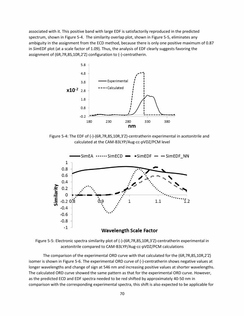
70

associated with it. This positive band with large EDF is satisfactorily reproduced in the predicted

spectrum, shown in Figure 5-4. The similarity overlap plot, shown in Figure 5-5, eliminates any

ambiguity in the assignment from the ECD method, because there is only one positive maximum of 0.87

in SimEDF plot (at a scale factor of 1.09). Thus, the analysis of EDF clearly suggests favoring the

assignment of (6R,7R,8S,10R,2'Z) configuration to (-)-centratherin.

Figure 5-4: The EDF of (-)-(6R,7R,8S,10R,3'Z)-centratherin experimental in acetonitrile and

calculated at the CAM-B3LYP/Aug-cc-pVDZ/PCM level

Figure 5-5: Electronic spectra similarity plot of (-)-(6R,7R,8S,10R,3'Z)-centratherin experimental in

acetonitrile compared to CAM-B3LYP/Aug-cc-pVDZ/PCM calculations

The comparison of the experimental ORD curve with that calculated for the (6R,7R,8S,10R,2'Z)

isomer is shown in Figure 5-6. The experimental ORD curve of (-)-centratherin shows negative values at

longer wavelengths and change of sign at 546 nm and increasing positive values at shorter wavelengths.

The calculated ORD curve showed the same pattern as that for the experimental ORD curve. However,

as the predicted ECD and EDF spectra needed to be red shifted by approximately 40-50 nm in

comparison with the corresponding experimental spectra, this shift is also expected to be applicable for

71

the calculated ORD curve. For this reason, the larger magnitude for SOR at 365nm in the experimental

data can only be reproduced when the calculations are performed at less than 365 nm. Except for this

difference, the trends seen in the experimental and predicted ORD values are considered to be in

agreement, thereby implying the (6R,7R,8S,10R,2'Z) AC assignment for (-)-centratherin.

Figure 5-6: The ORD of (-)-(6R,7R,8S,10R,3'Z)-centratherin experimental in acetonitrile and calculated at


The experimental VA and VCD spectra of (-)-centratherin are compared to the corresponding

predicted spectra for the (6R,7R,8S,10R,2'Z) isomer in Figure 5-7 and Figure 5-8. To co-display the

experimental and calculated VCD spectra on the same y-axis scale, the experimental VCD intensities

were scaled by 0.5. Visual comparison indicates excellent agreement between experimental and

calculated spectra, for VA as well as VCD.

Figure 5-7: The VA spectrum of (-)-(6R,7R,8S,10R,3'Z)-centratherin experimental in acetonitrile and

calculated at the B3LYP/Aug-cc-pVDZ/PCM level

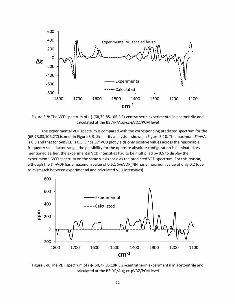
72

Figure 5-8: The VCD spectrum of (-)-(6R,7R,8S,10R,3'Z)-centratherin experimental in acetonitrile and


The experimental VDF spectrum is compared with the corresponding predicted spectrum for the

(6R,7R,8S,10R,2'Z) isomer in Figure 5-9. Similarity analysis is shown in Figure 5-10. The maximum SimVA

is 0.8 and that for SimVCD is 0.5. Since SimVCD plot yields only positive values across the reasonable

frequency scale factor range, the possibility for the opposite absolute configuration is eliminated. As

mentioned earlier, the experimental VCD intensities had to be multiplied by 0.5 to display the

experimental VCD spectrum on the same y-axis scale as the predicted VCD spectrum. For this reason,

although the SimVDF has a maximum value of 0.62, SimVDF_NN has a maximum value of only 0.2 (due

to mismatch between experimental and calculated VCD intensities).

Figure 5-9: The VDF spectrum of (-)-(6R,7R,8S,10R,3'Z)-centratherin experimental in acetonitrile and


73

Figure 5-10: Vibrational similarity plot of (-)-(6R,7R,8S,10R,3'Z)-centratherin experimental in acetonitrile

compared to B3LYP/Aug-cc-pVDZ/PCM calculations

Conclusion Starting from the reported relative configuration of (-)-centratherin, its absolute configuration is

determined by the combined application of different chiroptical spectroscopic properties, namely ECD,

EDF, ORD, VCD, and VDF. The prediction of these chiroptical spectroscopic properties matched the

corresponding experimental data quite well. The quantification of agreement between experimental

and calculated spectra is assessed through similarity overlap analysis. All these analyses confirmed the

AC of naturally occurring (-)-centratherin as (6R,7R,8S,10R,2'Z).

Experimental The isolation and characterization of centratherin was carried out by our Brazilian collaborators

and has been described in the literature.125

The optical rotation data at six different wavelengths, namely, 633, 589, 546, 436, 405, and 365

nm, were measured in CH3CN, at a concentration of 2.76 mg/mL, using an Autopol IV polarimeter. ECD

spectra in the ~187−400 nm region were measured in CH3CN, at a concentration of 2.32 mg/mL, using a

Jasco J-720 spectrometer using 1 and 0.1 mm quartz cells. The reported Δε values are expressed in units

of L mol−1 cm−1. VCD spectra in the 1800−1100 cm−1 region were measured in CH3CN, at concentration of

23 mg/mL (and 9 mg/mL for the carbonyl region) using a ChiralIR spectrometer (BioTools Inc.) and a 200

μm path length SL3 cell equipped with BaF2 windows. The reported Δε values are expressed in units of L

mol−1 cm−1.

The structure of centratherin, with the proposed relative configuration132 (6R,7R,8S,10R,2'Z),

was constructed using the molecular editor and visualizer program Avogadro v.1.1.0, and a

conformational analysis was carried out with the MMFF94s force field133 using the Conflex package.124

These geometries, within 25 kcal/mol energy range, were reoptimized using the semi-empirical PM6

method available in GAUSSIAN 09. The resulting geometries, within 5 kcal/mol energy range, were

reoptimized using DFT at the B3LYP/6-31G(d) level of theory. The conformers, within 3 kcal/mol energy

74

range, had their geometries reoptimized at B3LYP/Aug-cc-pVDZ level of theory. These reoptimized

structures identified 16 low energy conformers (See Supporting Information for optimized Cartesian

coordinates of these conformers) and all of these structures were used for ORD, ECD, and VCD

calculations. The long range corrected CAM-B3LYP level was used for ORD and ECD, while the B3LYP

level was used for VCD, all of them with Dunning’s Aug-cc-pVDZ correlation consistent basis set with

augmented functions with the GAUSSIAN 09 series of programs. The polarizable continuum model

(PCM)134 was used to take the influence of solvent (CH3CN) into consideration when using DFT methods.

The calculated spectra were obtained by weighting the individual spectra of conformers, according to

Boltzmann populations determined using Gibbs energies.

75

Chapter 6 The AC of (+)-3-ishwarone


de Janeiro, Brazil. For full details, please refer to the completed work as it appears in The Journal of

Natural Products.135

Introduction In cases where compounds have more than one chiral center, determination of the AC by

chiroptical means can be complicated because diastereomers (non-mirror image stereo-isomers) of a

chiral compound can have similar chiroptical spectra. Therefore even the most reliable quantum

chemical predictions may not offer enough discrimination to distinguish between them.136 Despite

developments in chiroptical spectroscopy and QC methodologies, determination of the ACs of natural

products with complex structures is one of the most challenging tasks in current research.137 If the

correct diastereomer can be determined by X-ray, NMR, or synthetic studies, chiroptical spectroscopic

methods can come to the rescue if many chiroptical methods are simultaneously employed for

structural characterization.138 In this chapter, chiroptical methods are used to determine the AC of the

natural product 3-ishwarone distinguishing its 4 possible diastereomers.

Molecular vibrations are inherently sensitive to the structural differences and, therefore,

chiroptical spectroscopic methods based on molecular vibrations (VCD and ROA) offer sensitive probes

to molecular structure. Diastereomers can in principle give different VCD and ROA spectra (as well as

parent VA or Raman spectra), although the extent of differences that can be seen for diastereomers

depends on the individual chiral systems.136 An advantage associated with vibrational optical activity is

that the number of vibrational transitions in the experimentally accessible region is far greater than that

of electronic transitions. As a result more stringent evaluation of structural predictions can be

undertaken by comparing the experimental vibrational spectra with those predicted for all possible

structures using modern quantum chemical theories. By using combination of chiroptical methods,

supported by calculations and numerical measures of similarity, the AC is discernible from a number of

possible diastereomers. This chapter will illustrate how chiroptical methods can be a powerful tool for

molecular structure determination.

In previous work,139 the isolation and determination of the relative configurations of several

chiral centers of a rare sesquiterpene 3-ishwarone140 were determined, the structure shown in Figure

6-1. The relative configurations at carbons 1, 2, 9 and 11 were unambiguously determined139 using NMR

data. Then the relative configurations at carbons 4 and 5 were evaluated by comparisons of

experimental and calculated spectra of four possible diastereomers: (1R,2S,4S,5R,9R,11R);

(1R,2S,4S,5S,9R,11R); (1R,2S,4R,5R,9R,11R); and (1R,2S,4R,5S,9R,11R) labeled A,B,C, and D respectively

(see Figure 6-1), but the NMR and IR analyses were not able to determine the relative configuration.

However the VCD signals in the fingerprint region are very sensitive to molecular structure and can allow

for the determination of the relative configuration of 3-ishwarone.

76

Figure 6-1: 3-Ishiwarone

Results and Discussion

ECD and EA spectra were measured in the 190-350 nm region in acetonitrile, and are compared

to the corresponding predicted spectra for all four possible diastereomers in Figure 6-2 and Figure 6-3.

In addition to the weak negative ECD band at ~300 nm, the experimental ECD spectrum shows a strong

positive ECD band at ~210 nm, corresponding to the EA band at ~205 nm. The negative ECD band is

reproduced in the calculations for all four diastereomers. Similarly the positive ECD band at ~200 nm is

also reproduced for all four diastereomers, even though the predicted position is shifted among

diastereomers. Based on this information alone, it is not possible to select one diastereomer to have

reproduced the experimental ECD spectrum better than the others.

77

Figure 6-2: Comparison of experimental EA spectrum of (+)-3-ishwarone in acetonitrile (scaled by 0.16)

with those predicted for four diastereomers calculated at the B3LYP/Aug-cc-pVDZ/PCM level

Figure 6-3: Comparison of experimental ECD spectrum of (+)-3-ishwarone in acetonitrile (scaled by 0.16)


0.00E+00

2.00E+04

4.00E+04

150 200 250 300 350

ε

nm

Experiment

A=(1R,2S,4S,5R,9R,11R)

B=(1R,2S,4S,5S,9R,11R)

C=(1R,2S,4R,5R,9R,11R)

D=(1R,2S,4R,5S,9R,11R)

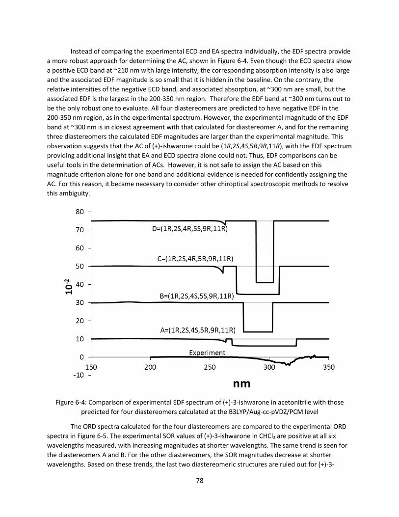
78

Instead of comparing the experimental ECD and EA spectra individually, the EDF spectra provide

a more robust approach for determining the AC, shown in Figure 6-4. Even though the ECD spectra show

a positive ECD band at ~210 nm with large intensity, the corresponding absorption intensity is also large

and the associated EDF magnitude is so small that it is hidden in the baseline. On the contrary, the

relative intensities of the negative ECD band, and associated absorption, at ~300 nm are small, but the

associated EDF is the largest in the 200-350 nm region. Therefore the EDF band at ~300 nm turns out to

be the only robust one to evaluate. All four diastereomers are predicted to have negative EDF in the

200-350 nm region, as in the experimental spectrum. However, the experimental magnitude of the EDF

band at ~300 nm is in closest agreement with that calculated for diastereomer A, and for the remaining

three diastereomers the calculated EDF magnitudes are larger than the experimental magnitude. This

observation suggests that the AC of (+)-ishwarone could be (1R,2S,4S,5R,9R,11R), with the EDF spectrum

providing additional insight that EA and ECD spectra alone could not. Thus, EDF comparisons can be

useful tools in the determination of ACs. However, it is not safe to assign the AC based on this

magnitude criterion alone for one band and additional evidence is needed for confidently assigning the

AC. For this reason, it became necessary to consider other chiroptical spectroscopic methods to resolve

this ambiguity.

Figure 6-4: Comparison of experimental EDF spectrum of (+)-3-ishwarone in acetonitrile with those

predicted for four diastereomers calculated at the B3LYP/Aug-cc-pVDZ/PCM level

The ORD spectra calculated for the four diastereomers are compared to the experimental ORD

spectra in Figure 6-5. The experimental SOR values of (+)-3-ishwarone in CHCl3 are positive at all six

wavelengths measured, with increasing magnitudes at shorter wavelengths. The same trend is seen for

the diastereomers A and B. For the other diastereomers, the SOR magnitudes decrease at shorter

wavelengths. Based on these trends, the last two diastereomeric structures are ruled out for (+)-3-

79

ishwarone. Even though both ORD and ECD originate from the same electronic transitions, ORD can

provide discrimination among diastereomers in instances where ECD cannot. Thus, the use of both ECD

and ORD simultaneously is advantageous for chiral molecular structure determination.

Figure 6-5: Comparison of experimental ORD spectrum of (+)-3-ishwarone in chloroform with those


The experimental VA and VCD spectra are compared to those calculated for the four

diastereomers in Figure 6-6 and Figure 6-7. The VDF spectrum is shown in Figure 6-8. To present

experimental and calculated spectra together, the experimental VCD and VDF spectra were scaled by

0.5. Since there are numerous vibrational bands in the 1600-1000 cm-1 region, an untrained eye would

claim all spectra appear similar and it would be difficult to visually identify the differences among the

spectra of the diastereomers. This problem is avoided through similarity analysis by numerically

evaluating the overlap among experimental and predicted spectra for the VA, VCD, and VDF spectra,

shown in Figure 6-9.

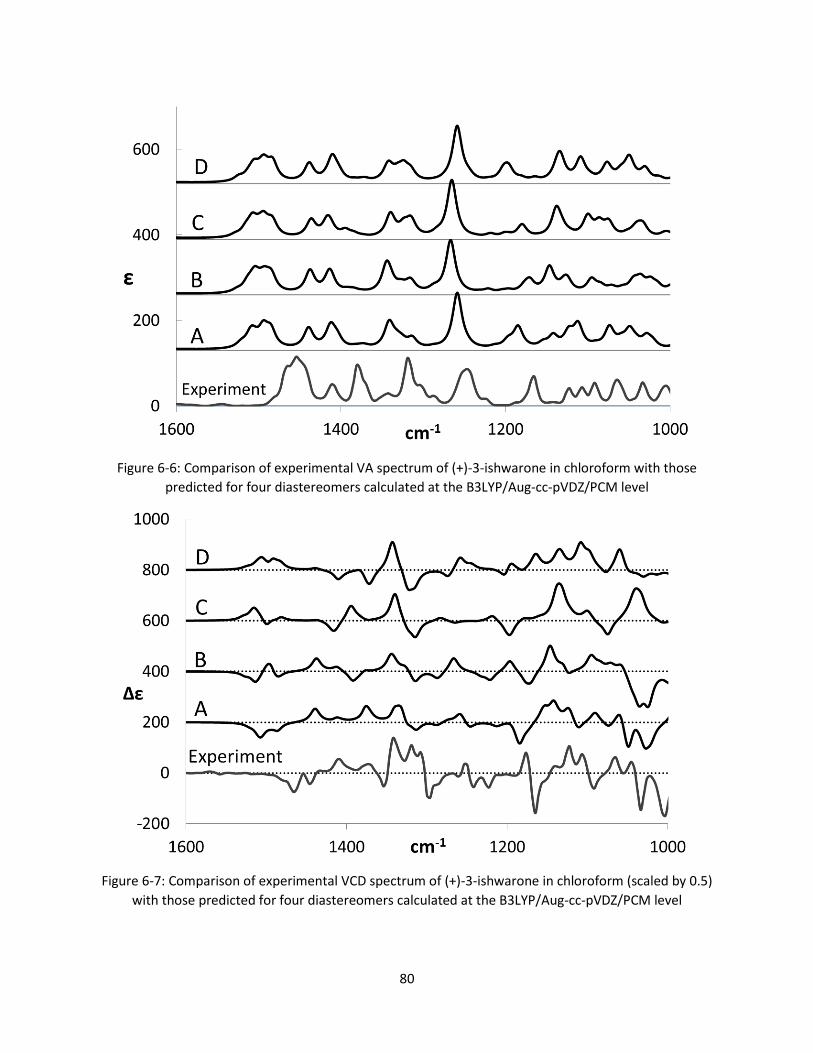
80

Figure 6-6: Comparison of experimental VA spectrum of (+)-3-ishwarone in chloroform with those


Figure 6-7: Comparison of experimental VCD spectrum of (+)-3-ishwarone in chloroform (scaled by 0.5)


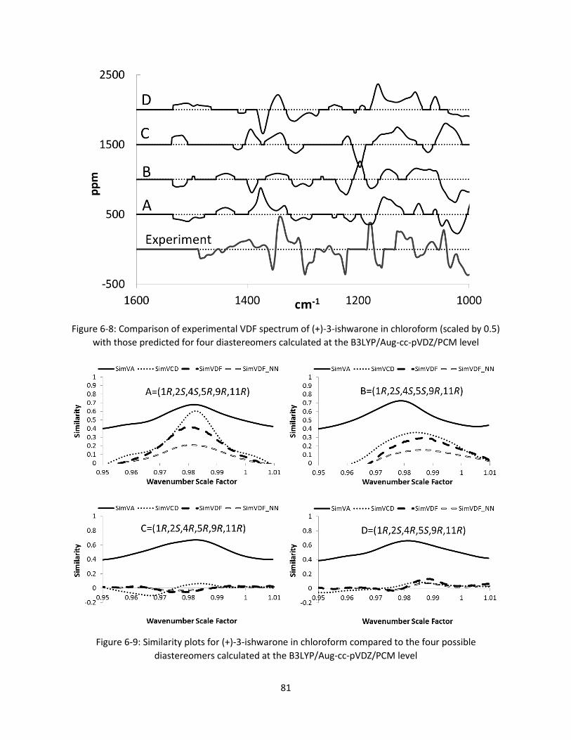
81

Figure 6-8: Comparison of experimental VDF spectrum of (+)-3-ishwarone in chloroform (scaled by 0.5)


Figure 6-9: Similarity plots for (+)-3-ishwarone in chloroform compared to the four possible

diastereomers calculated at the B3LYP/Aug-cc-pVDZ/PCM level

82

The similarity of the experimental VA spectrum with the corresponding calculated

spectra is ~0.7 for all four diastereomers and, therefore, VA spectra cannot discriminate among

the four diastereomers of 3-ishwarone. The similarity of the experimental VCD spectrum with

the corresponding calculated spectrum is ~0.6 for diastereomer A, 0.36 for diastereomer B, and

less than 0.1 for diastereomers C and D. The similarity of the experimental VDF spectrum with

the corresponding calculated spectrum is 0.41 for diastereomer A and 0.29 for diastereomer B,

and less than 0.1 for the remaining two diastereomers. From these comparisons, it can be

concluded that the predicted VCD and VDF spectra for the diastereomer A have the greatest

similarities with the corresponding experimental observations, strongly suggesting an AC of

(1R,2S,4S,5R,9R,11R).

Conclusion The comparison of the experimental ECD spectrum with those calculated for four

diastereomers could not establish the AC of (+)-3-ishwarone. However, the comparison of

corresponding EDF spectra indicates that the AC of (+)-3-ishwarone may be

(1R,2S,4S,5R,9R,11R). Analysis of the experimental ORD spectrum with those calculated for four

diastereomers rules out the last two diastereomers as likely candidates and narrows the choice

to the (1R,2S,4S,5R,9R,11R) and (1R,2S,4S,5S,9R,11R) diastereomers. Analysis of the

experimental VCD spectrum with those calculated for the four diastereomers also rules out the

last two diastereomers as likely candidates and provides better similarity with the VCD spectra

calculated for the (1R,2S,4S,5R,9R,11R) diastereomer. Thus, based on analyses of the three

different chiroptical data sets, the AC of (+)-3-ishwarone is unequivocally assigned as

(1R,2S,4S,5R,9R,11R).

Experimental The isolation and characterization of Ishwarone was carried out by our Brazilian

collaborators and has been described in the literature.135

The SOR data at six different wavelengths, namely 633, 589, 546, 436, 405, and 365 nm

were determined in CHCl3 using an Autopol IV polarimeter. ECD spectra were measured in the

190-350 nm region in acetonitrile solutions using a Jasco J-720 spectrometer and 0.1 mm quartz

cell. VCD spectra in the 2000-900 cm-1 region were measured for CDCl3 solutions (11.6 mg in

100 μL solvent) using a ChiralIR spectrometer (BioTools Inc) and a 100 micron path length SL3

cell with BaF2 windows. The reported Δε values are expressed in units of L mol-1 cm-1.

The structures of the four diastereomers were constructed and their geometries were

optimized (with MMFF94 force-field) using the free molecular editor and visualizer program

Avogadro, which was also used for conformational analysis. These geometries were re-

optimized using DFT at the B3LYP/6-31G(d) level of theory and then re-optimized at the

B3LYP/Aug-cc-pVDZ/PCM level for ORD, ECD, and VCD calculations using Gaussian 09.

83

Chapter 7 The AC of (‒)-Hypogeamicin B

This work was completed in collaboration with Professor Brian Bachmann, Vanderbilt University. For full

details, please refer to the completed work as it appears in The Journal of Natural Products.141

Introduction In this chapter, the determination of the AC of a novel secondary metabolite from a cave-

derived actinomycete, Nonomuraea specus (Gen-Bank KJ209502) is presented. This natural product,

named hypogeamicin B, presented a challenge for traditional means of chiroptical comparison and

greatly benefited from the use of the VDF and EDF spectra as well as numerical evaluation of similarity.

Caves in southern North America are ancient subterranean structures, which host so-called

hypogean, or underground, ecosystems that can be very distinct from those found on the surface of the

earth. These ecosystems are distinct in that they have virtually no sunlight, high relative humidity,

constant temperature, and very low dissolved carbon. The unique environmental properties of these

ecosystems have prompted the investigation of the secondary metabolic capacity of cultivatable

hypogean actinomycetes, as this class of microorganisms is a proven prolific source of interesting

secondary metabolites.142

Figure 7-1: Hypogeamicins A−D

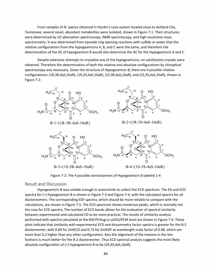
84

From samples of N. specus obtained in Hardin’s cave system located close to Ashland City,

Tennessee, several novel, abundant metabolites were isolated, shown in Figure 7-1. Their structures

were determined by UV absorption spectroscopy, NMR spectroscopy, and high resolution mass

spectrometry. It was determined from epoxide ring opening reactions with sulfide or water that the

relative configurations from the hypogeamicins A, B, and C were the same, and therefore the

determination of the AC of hypogeamicin B would also determine the AC for the Hypogeamicin A and C.

Despite extensive attempts to crystalize any of the hypogeamicins, no satisfactory crystals were

obtained. Therefore the determination of both the relative and absolute configurations by chiroptical

spectroscopy was necessary. Given the structure of Hypogeamicin B, there are 4 possible relative

configurations: (1R,3R,4aS,10aR), (1R,3S,4aS,10aR), (1S,3R,4aS,10aR), and (1S,3S,4aS,10aR), shown in

Figure 7-2.

Figure 7-2: The 4 possible stereoisomers of Hypogeamicin B labeled 1-4

Result and Discussion Hypogeamicin B was soluble enough in acetonitrile to collect the ECD spectrum. The EA and ECD

spectra for (‒)-hypogeamicin B is shown in Figure 7-3 and Figure 7-4, with the calculated spectra for all

diastereomers. The corresponding EDF spectra, which should be more reliable to compare with the

calculations, are shown in Figure 7-5. The ECD spectrum shows numerous peaks, which is normally not

the case for ECD spectra. The number of ECD bands allows for the evaluation of spectral similarity

between experimental and calculated CD to be more practical. The results of similarity analysis

performed with spectra calculated at the B3LYP/Aug-cc-pVDZ/PCM level are shown in Figure 7-6. These

plots indicate that similarity with experimental ECD and dissymmetry factor spectra is greater for the B-2

diastereomer, with 0.69 for SimECD and 0.73 for SimEDF at wavelength scale factor of 0.96, which are

more than 0.2 higher than any other configuration. Also the alignment of the maxima in the Sim

funtions is much better for the B-2 diastereomer. Thus ECD spectral analysis suggests the most likely

absolute configuration of (‒)-hypogeamicin B to be (1R,3S,4aS,10aR).

85

Figure 7-3: The EA spectra for (‒)-hypogeamicin B in acetonitrile with those predicted for the four


Figure 7-4: The ECD spectra for (‒)-hypogeamicin B in acetonitrile with those predicted for the four


86

Figure 7-5: The EDF spectra for (‒)-hypogeamicin B in acetonitrile with those predicted for the four


Figure 7-6: Electronic CD similarity analysis (‒)-hypogeamicin B in acetonitrile with those predicted for

the four diastereomers calculated at the B3LYP/Aug-cc-pVDZ/PCM level

87

The number of hydrogen bonding groups in Hypogeamicin B proved problematic, as it was not

sufficiently soluble in acetonitrile for VCD measurements. VCD measurements required the use of the

strong hydrogen bonding solvent DMSO, making extensive studies with the solute-solvent complexes

necessary. There are also numerous conformations from the substituents at the 1, 7, and 3 positions,

and the possibility for two internal hydrogen bonds create a large number of configurations that must

be considered. Five different models of solvation were chosen to represent hypogeamicin B in DMSO,

with combinations of internal hydrogen bonding and DMSO complexation, all including the PCM to

incorporate non-specific solvent effects, shown in Figure 7-7.

Figure 7-7: The solvation models chosen to represent hypogeamicin B

The experimental VCD spectra for (‒)-hypogeamicin B in DMSO are shown in Figure 7-8 with the

calculated spectra using the DMSO/Closed solvation model; The corresponding VA and VDF are shown in

Figure 7-9 and Figure 7-10 respectively. The DMSO/Closed solvation model provided the best agreement

out of any of the solvation models, as demonstrated by the similarity plot shown in Figure 7-11. Instead

of showing the remaining 16 similarity plots, the maximum Sim values are presented in Table 7-1.

88

Figure 7-8: VCD spectra for (‒)-hypogeamicin B in DMSO compared to DMSO/Closed solvation model

Figure 7-9: VA spectra for (‒)-hypogeamicin B in DMSO compared to DMSO/Closed solvation model

89

Figure 7-10: VDF spectra for (‒)-hypogeamicin B in DMSO compared to DMSO/Closed solvation model

Figure 7-11: Vibrational similarity plots for (‒)-hypogeamicin B in DMSO compared to DMSO/Closed

solvation model

90

VCD VDF

Diastereomer 1 2 3 4 1 2 3 4

Closed/Closed 0.154 0.485 0.099 0.238 0.085 0.269 0.062 0.181

Closed/Open 0.069 0.045 0.078 0.145 0.182 0.355 0.102 0.149

DMSO/Closed 0.136 0.483 0.140 0.275 0.129 0.387 0.098 0.225

DMSO/Open 0.090 0.097 0.145 0.169 0.142 0.440 0.083 0.224

DMSO/DMSO 0.150 0.238 0.174 0.120 0.210 0.365 0.115 0.048

SUM 0.600 1.348 0.635 0.946 0.748 1.817 0.460 0.828

Table 7-1: Maximum similarity ratings from all solvation models for (‒)-hypogeamicin B in DMSO

From the VCD and VDF similarity analyses, the best agreement is found for B-2 suggesting an

absolute configuration of (1R,3S,4aS,10aR). Considering all solvent models, though the VCD may not

match between theory and experiment, the VDF compares only the most robust vibrations that are less

likely to be shifted by solvent interactions. Accordingly the VDF for B-2 always matches the experimental

spectrum better than any other diastereomer, and always with similarity ratings better than 0.25.

Conclusion Despite strong solute interactions, the chiroptical spectra for (‒)-hypogeamicin B were

accurately reproduced through quantum chemical calculations. The use of the VDF and EDF along with

similarity analysis allowed for the designation of the AC of (‒)-hypogeamicin B to be (1R,3S,4aS,10aR). In

this case, chiroptical spectroscopy allowed for the determination of the correct diastereomer of a

compound containing multiple chiral centers.

Experimental The chiroptical measurements were conducted by Dr. Ganesh Shanmugam. All QC calculations

and conformational analyses were carried by Dr. Giovanni Scalmani of Gaussian Inc and fully described

in the literature.141 In summary, VCD calculations were performed on the optimized geometries for each

solvent model at the B3LYP/6-31G(d)/PCM level. TD-DFT calculations of the first 50 states were

performed at the B3LYP/Aug-cc-pVDZ/PCM level on the 4 lowest energy conformers (using the B3LYP/6-

31G(d)/PCM geometries); electronic transitions covered the range 340-170 nm.

91

Chapter 8 The AC of (‒)-Agathisflavone


de Janeiro, Brazil. The relevant experimental details are available in the appendices.

Introduction When calculating the chiroptical properties of polar compounds with many hydrogen bonding

groups, considerations must be made for the solvent-solute interactions. In cases where strong

hydrogen bonding solvents are necessary, great care must be taken to ensure any conclusions are valid.

In this chapter, the determination of the AC of the natural product agathisflavone, a dimeric flavonoid, is

presented with extensive modeling of solvent interactions.

Flavonoids are naturally occurring secondary metabolites found in plants that have been long

studied for their numerous biological activities and medicinal properties.143 Atropisomerism in

biflavones has been known since the sixties.144 However, these compounds are still puzzling in the sense

that they are chiral molecules with molecular dissymmetry. The stereochemical determination of these

natural products remained unknown for over 20 years after their first isolation in optically active form.

Even in the current times, the determination of the axial chirality remains a challenging problem within

this class of natural products, since there are only a few examples of AC determination of biaryl axis

containing natural compounds and many of them are not even recognized (isolated) as optically

active.145 The first stereochemical analysis for this class of compounds was made by the application of

the exciton chirality method for ECD.146 However during the nineties, Harada and co-workers showed

how difficult the application of the exciton chirality method for biflavones can be.147

Figure 8-1: Flavone backbone and Agathisflavone

In this chapter, the first natural occurrence of optically active biflavonoid agathisflavone is

described. Agathisflavone is a biflavone-type dimeric flavonoid interconnected through a chemical bond

between C-6 (ring A) and C-8'' (ring D), see Figure 8-1. This compound was isolated from Schinus

terebinthifolius Raddi (Anacardiaceae), known as Aroeira or Brazilian pepper tree, which is a small tree

with small globose fruits (red drupes). Brazilian pepper tree has been used in the Brazilian folk medicine

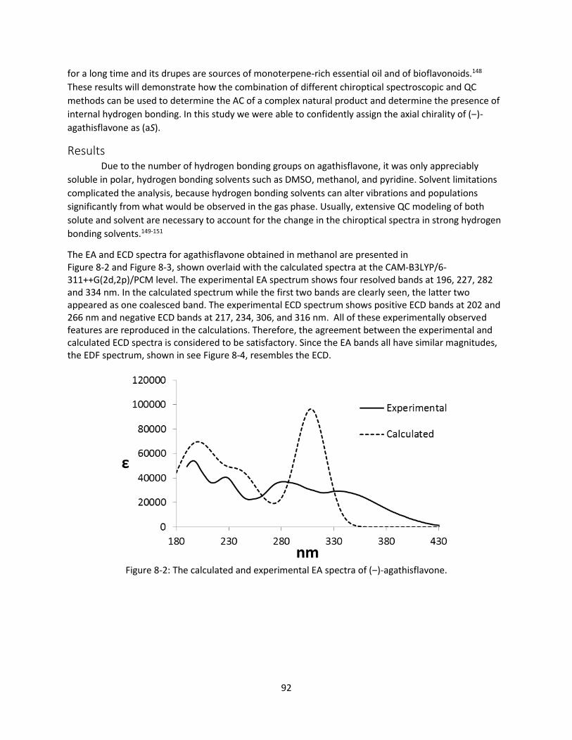
92

for a long time and its drupes are sources of monoterpene-rich essential oil and of bioflavonoids.148

These results will demonstrate how the combination of different chiroptical spectroscopic and QC

methods can be used to determine the AC of a complex natural product and determine the presence of

internal hydrogen bonding. In this study we were able to confidently assign the axial chirality of (‒)-

agathisflavone as (aS).

Results Due to the number of hydrogen bonding groups on agathisflavone, it was only appreciably

soluble in polar, hydrogen bonding solvents such as DMSO, methanol, and pyridine. Solvent limitations

complicated the analysis, because hydrogen bonding solvents can alter vibrations and populations

significantly from what would be observed in the gas phase. Usually, extensive QC modeling of both

solute and solvent are necessary to account for the change in the chiroptical spectra in strong hydrogen

bonding solvents.149-151

The EA and ECD spectra for agathisflavone obtained in methanol are presented in Figure 8-2 and Figure 8-3, shown overlaid with the calculated spectra at the CAM-B3LYP/6-311++G(2d,2p)/PCM level. The experimental EA spectrum shows four resolved bands at 196, 227, 282 and 334 nm. In the calculated spectrum while the first two bands are clearly seen, the latter two appeared as one coalesced band. The experimental ECD spectrum shows positive ECD bands at 202 and 266 nm and negative ECD bands at 217, 234, 306, and 316 nm. All of these experimentally observed features are reproduced in the calculations. Therefore, the agreement between the experimental and calculated ECD spectra is considered to be satisfactory. Since the EA bands all have similar magnitudes, the EDF spectrum, shown in see Figure 8-4, resembles the ECD.

Figure 8-2: The calculated and experimental EA spectra of (‒)-agathisflavone.

93

Figure 8-3: The experimental ECD spectrum of (‒)-agathisflavone compared to the calculated spectrum

with the (aS) AC at the CAM-B3LYP/6-311++G(2d,2p)/PCM level

Figure 8-4: The experimental EDF spectrum of (‒)-agathisflavone compared to the calculated spectrum


The relative energies and rotational strengths of the electronic transitions are not perfectly

matched. The wide range of the electronic region being probed prevents one scale factor from providing

a good match between calculated and experimentally observed transition wavelengths in the entire

region. The deficiencies in the functional used, and/or in the PCM model to account for solvent effects,

could also have caused the mismatches noted above. These observations are reflected in the smaller

than desired similarity overlap values of 0.28 for SimECD, 0.40 for SimEDF, and 0.75 for SimEA, similarity

plot shown in Figure 8-5. The similarity analyses cannot be blindly used as a replacement for the visual

comparison criterion. The reasonable agreement of experimentally observed ECD and EDF bands with

those in the calculations strongly supports the assignment of (aS) configuration for (‒)-agathisflavone.

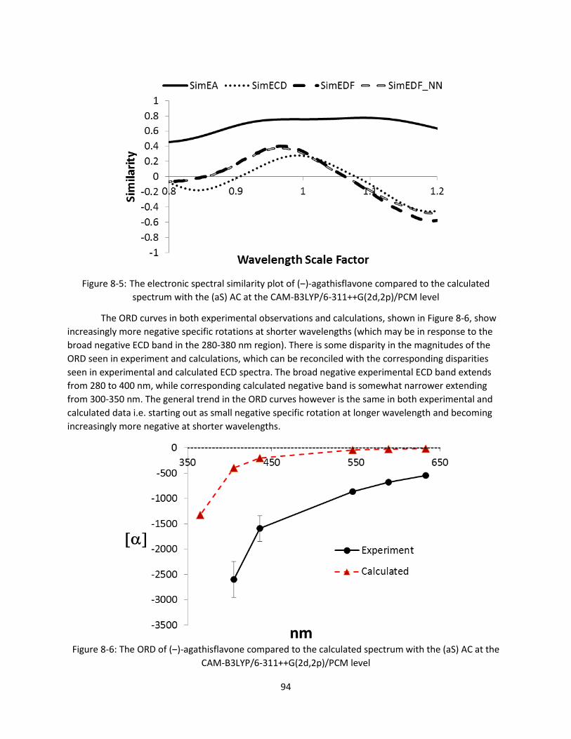
94

Figure 8-5: The electronic spectral similarity plot of (‒)-agathisflavone compared to the calculated

spectrum with the (aS) AC at the CAM-B3LYP/6-311++G(2d,2p)/PCM level

The ORD curves in both experimental observations and calculations, shown in Figure 8-6, show

increasingly more negative specific rotations at shorter wavelengths (which may be in response to the

broad negative ECD band in the 280-380 nm region). There is some disparity in the magnitudes of the

ORD seen in experiment and calculations, which can be reconciled with the corresponding disparities

seen in experimental and calculated ECD spectra. The broad negative experimental ECD band extends

from 280 to 400 nm, while corresponding calculated negative band is somewhat narrower extending

from 300-350 nm. The general trend in the ORD curves however is the same in both experimental and

calculated data i.e. starting out as small negative specific rotation at longer wavelength and becoming

increasingly more negative at shorter wavelengths.

Figure 8-6: The ORD of (‒)-agathisflavone compared to the calculated spectrum with the (aS) AC at the

CAM-B3LYP/6-311++G(2d,2p)/PCM level

95

Although the agreement between experimental and calculated ECD spectra and between

experimental and calculated ORD curves for agathisflavone are satisfactory to suggest the AC

assignment, it is important to verify the AC assignments with other chiroptical methods whenever

possible. A complicating factor for agathisflavone, because the VCD spectral agreement is not as good as

the ECD. The VA, VCD, and VDF spectra for (‒)-agathisflavone are shown in Figure 8-7, Figure 8-8, and

Figure 8-9 respectively. While there are several large signals in the experimental VCD, visually they do

not match well with the patterns seen in the calculations. Though there is some match in the VCD, this

can be seen when the calculated spectrum is shifted to the left with a scale factor of 1.02; a similarity

plot using only the observable fingerprint region (up to 1500 cm-1) is shown in Figure 8-10. The problem

is that vibrational x-axis scale factors are almost always less than one, though external solvation effects

may change this. The shift is in all likeliness due to solvation effects from the strong hydrogen bonding

solvent. The solvation will change the Boltzmann population of the conformations and perturb the

vibrations to produce altered VA and VCD signals. This creates a problem because one does not know

how the normal modes will be affected without extensive calculations.

Figure 8-7: The experimental VA spectrum of (‒)-agathisflavone compared to the calculated spectrum at

the B3LYP/6-311++G(2d,2p)/PCM level

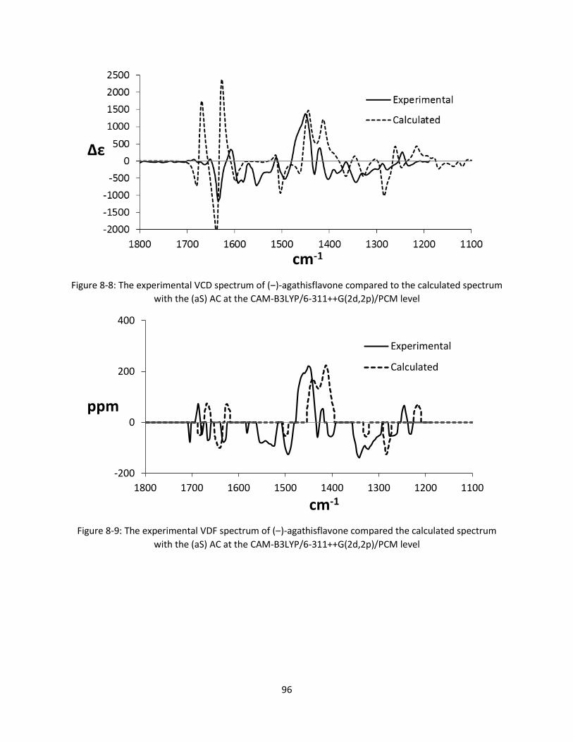
96

Figure 8-8: The experimental VCD spectrum of (‒)-agathisflavone compared to the calculated spectrum


Figure 8-9: The experimental VDF spectrum of (‒)-agathisflavone compared the calculated spectrum


-200

0

200

400

11001200130014001500160017001800

ppm

cm-1

Experimental

Calculated

97

Figure 8-10: The vibrational similarity plot comparing (‒)-agathisflavone to the (aS) AC at the B3LYP/6-311++G(2d,2p)/PCM level, comparing 1500-1200 cm-1

To explore the effects of solvent on the VCD spectrum of agathisflavone, MD simulations were

performed with agathisflavone in methanol followed by VCD calculations on the explicitly solvated

solute with both open and closed internal carbonyl-alcohol hydrogen bonds; an example snapshot is

shown in Figure 8-11. The time averaged spectra are shown in Figure 8-12 and Figure 8-13. The VDF

spectra from MD trajectories are compared in Figure 8-14. The open-OH bond trajectory has only a small

robust region and does not compare well with the experimental spectrum for VA, VCD, or VDF. The

closed-OH trajectory compares much better to the experiment, suggesting that the internal hydrogen

bonds are favored for agathisflavone dissolved in methanol.

Figure 8-11: A snapshot from the agathisflavone-methanol MD simulation. All methanol molecules

within 2.5 Å of a hydrogen bonding group are shown

98

Figure 8-12: The experimental VCD spectrum of (‒)-agathisflavone compared to the calculated spectra

with the (aS) AC from MD trajectories at the B3LYP/6-31G*/PCM level

Figure 8-13: The experimental VA spectrum of (‒)-agathisflavone compared to the calculated spectra

from MD trajectories at the B3LYP/6-31G*/PCM level

99

Figure 8-14: The experimental VDF spectrum of (‒)-agathisflavone compared to the calculated spectra

with the (aS) AC from MD trajectories at the B3LYP/6-31G*/PCM level

Figure 8-15: The vibrational similarity plot comparing (‒)-agathisflavone to the (aS) AC from closed-OH

MD trajectory at the B3LYP/6-31G*/PCM level, comparing 1500-1200 cm-1

Similarity analysis was performed considering only the observable vibrational transitions in

fingerprint region, shown in Figure 8-15. The similarity ratings are much higher and better aligned than

calculations that did not include explicit solvent, with maximum similarity ratings of 0.84, 0.60, and 0.61

for SimVA, SimVCD, and SimVDF respectively. Also the optimum x-axis scale factor is approximately 1.

Comparison between explicit and implicit (PCM) solvation models indicates that the vibrations that gave

rise to the VCD signals were shifted to higher frequency by solvent interactions, though this could have

very well not been the case. In this instance calculations including the explicit solvent improved the

confidence in the assignment of the AC of agathisflavone.

100

Conclusions For the natural product (‒)-agathisflavone, the VCD, ECD, and ORD spectra have been measured

and the absolute configuration has been determined to be (aS) by comparison with quantum chemical

calculations. The ECD spectrum of agathisflavone is quite complex, but comparison with quantum

chemical calculations provided excellent reproduction of all ECD bands. Solvent effects in the VCD

complicated the calculations, though extensive MD simulations and explicit solvent VCD calculations

improved the confidence in comparison considerably.

Experimental The isolation, characterization of agathisflavone was undertaken by our Brazilian collaborators

and details are provided in the Appendices.

The optical rotation (OR) data at five different wavelengths, namely, 633, 589, 546, 436, and 405

nm, were measured in methanol using an Autopol IV polarimeter. Three different concentrations, 0.03,

0.04 and 1.38 mg/ml, were used for these measurements. ECD spectra in the 190−450 nm region were

measured for methanol solution (1.38 mg/mL) using a Jasco J-720 spectrometer and 0.1 mm quartz cell.

The reported Δε values are in units of L mol−1 cm−1. VCD spectra in the 1800−1200 cm−1 region were

measured in CD3OD (32 mg/ml) and (CD3)2SO solutions using a ChiralIR spectrometer (BioTools Inc.) and

a 100 μm path length SL3 cell with BaF2 windows. The reported Δε values are in units of L mol−1 cm−1.

The structure of Agathisflavone was built in Avogadro107 and a systematic conformational search

was performed using CONFLEX124 with the MMFF94s133 force field, which produced 303 unique

conformations of both (aR) and (aS) chirality, as CONFLEX does not distinguish between atropisomers.

All conformations were optimized at the PM642 level of theory implemented in Gaussian 09,108 and 88

conformers within 5 kcal/mol of the lowest energy were optimized at the B3LYP/6-31G* level of theory

with methanol solvent modeled by PCM.37, 134 At this point all conformations with (aR) chirality were

inverted and matched to the (aS) to ensure all possible conformations would be used in further analysis.

Sequential optimizations at the B3LYP/6-311G** and B3LYP/6-311++G(2d,2p) theories with methanol

solvent modeled by PCM produced 43 conformers within 2 kcal/mol. Most of these conformations are

distinguished by minor permutations of the B and E rings, and the orientation of the B-ring and E-ring

hydroxyl groups (16 total permutations). These permutations were later seen to have little effect on the

ECD or ORD spectra.

In the optimization procedure, conformations that contained open hydrogen bonds were found

to be several kcal/mol higher in energy than the closed hydrogen bonding conformations, and were not

carried through. The modeling of solvation from hydrogen bonding solvent like methanol can be very

tedious, so in lieu of extensive analysis, open hydrogen bonding conformations were made (from the

lowest energy closed hydrogen bond conformer) and optimized using the same level of theory, and used

in chiroptical analysis.

ORD and ECD were calculated using CAM-B3LYP/6-311++G(2d,2p)/PCM. ECD was calculated for

the first 60 transitions. VCD calculations were performed at the same level of theory as that used for

optimizations.

For the explicit VCD calculations, MD simulations were performed using the GPU accelerated

version of Amber12 using the GAFF force field.38 The topology files were prepared using the program

101

Antechamber152 with charges from BCC fitting to the AM1 semi-empirical method153-154. To make a

parameter set with open OH bonds, a 5 kcal/mol dihedral force constant was added to the hydroxyl

groups at the 5 and 5’’ positions, forcing them to remain open. The system included Agathisflavone and

973 methanol in a square box, which was minimized for 500 steps and then equilibrated over 50 ps to a

temperature of 300 K and a pressure of 1 bar. MD simulations were run for 10 ns with an integration

time step of 2 fs with hydrogen bond lengths confined with SHAKE.155 Radial distribution functions were

calculated for all possible hydrogen bonding partners using cpptraj105 and the maximum hydrogen

bonding distance was inferred from the first minimum to be 2.5 Å.

Snapshots including the agathisflavone solute and methanol solvent within 2.5 Å of the

hydrogen bonding partners near the chiral center were exported at regular intervals of 200 ps (50

snapshots total). The snapshots were optimized at the B3LYP/6-31G*/PCM level keeping the solvent

molecules fixed, with harmonic frequencies and VCD intensities calculated at the same level with

deuterated solvent. Optimizations that did not converge were discarded. Convergence was determined

by averaging the VCD from first and second halves of the trajectories separately.

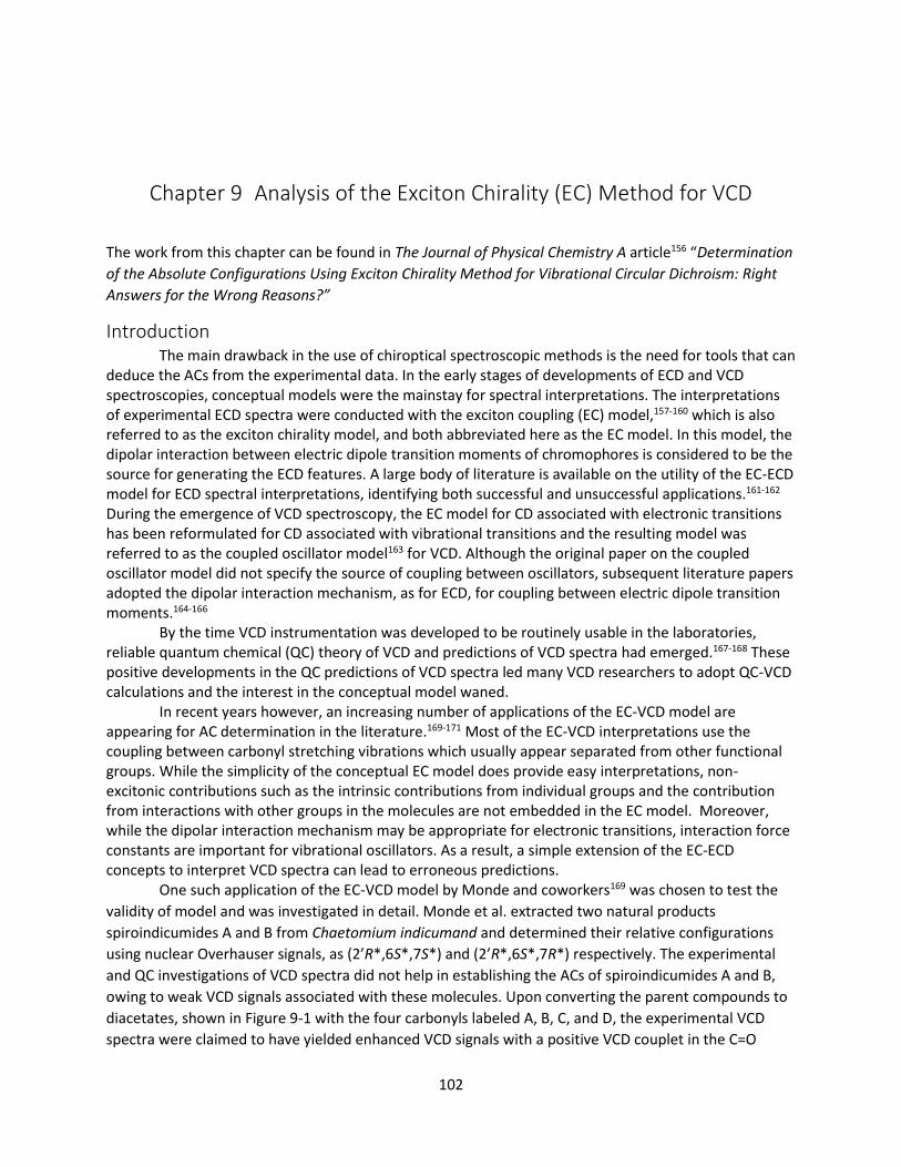
102

Chapter 9 Analysis of the Exciton Chirality (EC) Method for VCD

The work from this chapter can be found in The Journal of Physical Chemistry A article156 “Determination

of the Absolute Configurations Using Exciton Chirality Method for Vibrational Circular Dichroism: Right

Answers for the Wrong Reasons?”

Introduction The main drawback in the use of chiroptical spectroscopic methods is the need for tools that can

deduce the ACs from the experimental data. In the early stages of developments of ECD and VCD spectroscopies, conceptual models were the mainstay for spectral interpretations. The interpretations of experimental ECD spectra were conducted with the exciton coupling (EC) model,157-160 which is also referred to as the exciton chirality model, and both abbreviated here as the EC model. In this model, the dipolar interaction between electric dipole transition moments of chromophores is considered to be the source for generating the ECD features. A large body of literature is available on the utility of the EC-ECD model for ECD spectral interpretations, identifying both successful and unsuccessful applications.161-162 During the emergence of VCD spectroscopy, the EC model for CD associated with electronic transitions has been reformulated for CD associated with vibrational transitions and the resulting model was referred to as the coupled oscillator model163 for VCD. Although the original paper on the coupled oscillator model did not specify the source of coupling between oscillators, subsequent literature papers adopted the dipolar interaction mechanism, as for ECD, for coupling between electric dipole transition moments.164-166

By the time VCD instrumentation was developed to be routinely usable in the laboratories, reliable quantum chemical (QC) theory of VCD and predictions of VCD spectra had emerged.167-168 These positive developments in the QC predictions of VCD spectra led many VCD researchers to adopt QC-VCD calculations and the interest in the conceptual model waned.

In recent years however, an increasing number of applications of the EC-VCD model are appearing for AC determination in the literature.169-171 Most of the EC-VCD interpretations use the coupling between carbonyl stretching vibrations which usually appear separated from other functional groups. While the simplicity of the conceptual EC model does provide easy interpretations, non-excitonic contributions such as the intrinsic contributions from individual groups and the contribution from interactions with other groups in the molecules are not embedded in the EC model. Moreover, while the dipolar interaction mechanism may be appropriate for electronic transitions, interaction force constants are important for vibrational oscillators. As a result, a simple extension of the EC-ECD concepts to interpret VCD spectra can lead to erroneous predictions.

One such application of the EC-VCD model by Monde and coworkers169 was chosen to test the

validity of model and was investigated in detail. Monde et al. extracted two natural products

spiroindicumides A and B from Chaetomium indicumand and determined their relative configurations

using nuclear Overhauser signals, as (2’R*,6S*,7S*) and (2’R*,6S*,7R*) respectively. The experimental

and QC investigations of VCD spectra did not help in establishing the ACs of spiroindicumides A and B,

owing to weak VCD signals associated with these molecules. Upon converting the parent compounds to

diacetates, shown in Figure 9-1 with the four carbonyls labeled A, B, C, and D, the experimental VCD

spectra were claimed to have yielded enhanced VCD signals with a positive VCD couplet in the C=O

103

stretching region. A positive couplet refers to a pair of adjacent bands with positive band appearing at

lower energy (wavenumber) and negative band appearing at higher energy (wavenumber). Using the

conceptual EC model to interpret this VCD couplet, Monde and coworkers concluded that the AC at 2’

position should be (R) and hence the ACs of spiroindicumide A diacetate (SpA) and spiroindicumide B

diacetate (SpB) were assigned as (2’R,6S,7S) and (2’R,6S,7R) respectively.

Figure 9-1: The structure of (2’R,6S,7S)-spiroindicumide A diacetate and (2’R,6S,7R)-spiroindicumide B

diacetate, labeled SpA and SpB, and identifying the four carbonyl groups as A-D.

QC-VCD calculations were not undertaken for the SpA or SpB, and therefore the reported ACs

are subject to further verification. To verify the conclusions of the EC-VCD model, QC-VCD calculations

have been performed and used to analyze the extent of the EC contributions to VCD of SpA and SpB.

The Exciton Chirality (EC) Method For two identical interacting groups, the EC method is referred to as the degenerate EC (DEC)

method. For two non-equivalent interacting groups, the EC method is referred to as the non-degenerate

EC (NDEC) method. Here is presented a general automated method for evaluating the relevance of EC-

VCD phenomenon. From the QC predictions of VCD spectra for molecules containing carbonyl groups,

one can identify the two C=O stretching vibrations which are composed of coupled C=O stretching

coordinates in a given molecule. The electric dipole transition moment vector for the C=O stretching

vibration is chosen to point along the C=O bond.

The Dipolar interaction ,V12, is determined from the equation:

512

212121312

21012

3

R

uRRu

R

uuDV

( 9-1 )

where Au

and Bu

are the unit vectors associated with the two C=O bonds. The unit vectors point from C

to O atoms and the distance vector R12 is calculated from the center of mass of one C=O to another C=O

group. In the DEC model, the unperturbed energy of C=O stretching vibration is approximated as the

average of the energies of two C=O stretching vibrations in the QC calculations. The average

(theoretically unperturbed) dipole strength, Do, is approximated as the average of dipole strengths

predicted for those two coupled C=O stretching vibrations in the QC calculations.

SpA SpB

104

Using V12, the vibrational energies and the mixing between the two states in the EC-VCD model

are calculated from the equations:

2

1

2

1

12

0112

1202

11

c

cE

c

c

EEV

VEE ( 9-2 )

Which for identical groups gives energies 1201 VEEE . The rotational strengths are

calculated using:

2112210 uuRccDR o

( 9-3 )

The DEC model assumes degeneracy between the two groups and therefore both groups will

participate equally in the transition (the normalized coefficients 1c and 2c will have equal magnitudes).

In the NDEC model, both groups will not participate equally in the transition and there will be a

reduction in the rotational strength of the transition due to the coefficients 1c and 2c in Eq. ( 9-3 ). It is

important to realize that the NDEC-VCD can be diminished to a point that the intrinsic contributions

from other oscillators can dominate the VCD signal. The intrinsic contributions are not accounted for in

the EC model and can lead to the wrong conclusions. The amount that the EC-VCD contribution is

reduced can be estimated from:

50

50 21

.

. cc ( 9-4 )

Using modern QC calculations, the contribution of the EC-VCD can be determined using the interaction

force constants to determine the validity of the DEC-VCD approximations. All EC-VCD calculations were

carried out with an in-house written C++ computer program that directly extracts all the needed

information from Gaussian 09 output files.

The frequency order of symmetric and antisymmetric transitions in the EC-CD model is

determined by the sign of V12. However, for vibrational transitions, in the Wilson’s GF matrix method172

for solving the vibrational secular equation for two identical C=O stretching internal coordinates that do

not share common atoms, it can be shown that the anti-symmetric stretch will be lower in energy than

the symmetric stretch. The vibrational frequency separation of the two coupled C=O stretching

vibrations predicted by the DEC-VCD model would be 2V12. The comparison of this 2V12 with

experimentally observed frequency separation between the two C=O stretching vibrational transitions

will reveal if the dipolar coupling between electric dipole transition moments is adequate for explaining

the observed energy separation. The comparison of the sign of V12 with that of the interaction force

constants (f12) predicted in the QC calculations will reveal if dipolar interaction between electric dipole

transition moments provides the correct energy order for the two transitions.

To test the EC-VCD model, all the conformers of SpA and SpB were found using the MMFF94s force field (~700 each) in Conflex,124 which were then optimized using the progression of PM6 to B3LYP/6-31G*/PCM to B3LYP/TVZP/PCM levels of theory in Gaussian 09. VCD calculations were performed at the B3LYP/TVZP/PCM level. The populations or the dominant conformers of SpA and SpB

105

are shown in Table 9-1. Though the use of Gibbs energies alters the Boltzmann weights for the conformers, it does not significantly affect the averaged QC-VCD spectra.

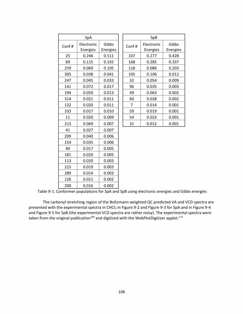
106

SpA SpB

Conf # Electronic Energies

Gibbs Energies

Conf # Electronic Energies

Gibbs Energies

25 0.246 0.511 107 0.277 0.428

69 0.115 0.192 168 0.285 0.337

259 0.069 0.105 118 0.086 0.203

305 0.038 0.041 105 0.106 0.012

247 0.045 0.033 32 0.054 0.009

141 0.072 0.017 96 0.035 0.003

194 0.050 0.013 49 0.063 0.002

314 0.021 0.011 60 0.028 0.002

132 0.020 0.011 7 0.014 0.001

333 0.017 0.010 59 0.019 0.001

11 0.020 0.009 54 0.023 0.001

213 0.069 0.007 31 0.012 0.001

41 0.027 0.007

209 0.040 0.006

154 0.035 0.006

40 0.017 0.005

181 0.020 0.005

113 0.020 0.003

215 0.019 0.003

289 0.014 0.003

126 0.011 0.002

200 0.016 0.002

Table 9-1: Conformer populations for SpA and SpB using electronic energies and Gibbs energies

The carbonyl stretching region of the Boltzmann weighted QC predicted VA and VCD spectra are presented with the experimental spectra in CHCl3 in Figure 9-2 and Figure 9-3 for SpA and in Figure 9-4 and Figure 9-5 for SpB (the experimental VCD spectra are rather noisy). The experimental spectra were taken from the original publication169 and digitized with the WebPlotDigitizer applet.173

107

Figure 9-2: The VA spectrum of SpA in CHCl3 with the calculated spectrum at the B3LYP/TZVP/PCM level

Figure 9-3: The VCD spectrum of SpA with the calculated spectrum at the B3LYP/TZVP/PCM level

108

Figure 9-4: The VA spectrum of SpB with the calculated spectrum at the B3LYP/TZVP/PCM level

Figure 9-5: The VCD spectrum of SpB with the calculated spectrum at the B3LYP/TZVP/PCM level

Results The population weighted spectra show a positive couplet in the C=O stretching region, for both

SpA and SpB, as also observed in their experimental spectra indicating that the AC used for calculations

may be assigned to the sample used for obtaining the experimental spectra. Thus the ACs concluded by

Monde and coworkers169 for diacetates of spiroindicumide A and B are supported by the current QC-VCD

calculations. However, the main question to be addressed is the relevance of the EC phenomenon for

the VCD couplet in the C=O stretching region.

With analysis of the normal mode displacements for the dominant conformers of SpA and SpB,

it was determined that the carbonyl A stretch occurs near 1825 cm-1 and is coupled to B, and that

109

carbonyl B stretch occurs near 1779 cm-1 and is coupled to A. The B3LYP/TZVP/PCM predicted

interaction force constants, vibrational frequencies and dissymmetry factors for the above mentioned

two C=O stretching modes of all low energy conformers of SpA are summarized in Table 9-2, and in

Table 9-3 for SpB.

SpA

B3LYP/TZVP/PCM EC-VCD Model

Higher frequency vibration

Lower frequency vibration



Conformer fAB cm-1 gi cm-1 gi VAB cm-1 gi cm-1 gi

25 0.012 1825 -0.7 1779 0.5 0.6 1803 -6.9 1801 2.3

69 0.010 1822 -0.6 1779 0.7 0.5 1801 -7.5 1800 2.1

259 0.031 1823 -0.8 1783 1.3 1.7 1805 -4.1 1801 3.6

305 0.029 1825 -1.2 1781 1.5 1.5 1804 -4.2 1801 3.5

247 0.030 1824 -1.0 1781 1.3 1.6 1804 -4.1 1801 3.6

141 0.026 1823 -0.6 1777 1.6 3.0 1803 -5.3 1797 2.7

194 0.025 1823 -0.7 1779 1.2 3.1 1804 -5.3 1798 2.7

314 0.036 1821 -0.9 1781 1.5 2.2 1803 -3.7 1799 3.9

132 0.026 1822 -0.6 1777 1.6 3.0 1802 -5.3 1796 2.7

333 0.032 1821 -1.2 1780 1.6 1.9 1803 -3.9 1799 3.7

11 0.023 1820 -0.5 1779 0.8 2.8 1802 -5.7 1797 2.6

213 0.034 1819 0.5 1768 -0.7 -4.6 1799 -2.7 1789 3.6

41 0.024 1822 -1.0 1778 1.2 2.8 1803 -5.4 1797 2.7

209 0.036 1821 0.6 1768 -0.8 -4.7 1799 -2.7 1790 3.6

154 0.037 1820 0.6 1769 -0.7 -4.6 1799 -2.7 1790 3.6

40 0.027 1822 -0.6 1776 1.6 3.1 1802 -5.2 1796 2.8

181 0.036 1821 0.5 1774 -0.8 -4.3 1801 -2.7 1793 3.5

113 0.038 1820 0.7 1770 -0.7 -4.6 1800 -2.7 1791 3.5

215 0.037 1820 0.7 1768 -0.8 -4.7 1799 -2.7 1790 3.6

289 0.025 1822 -0.9 1778 1.3 3.0 1803 -5.3 1797 2.7

126 0.034 1818 0.5 1768 -0.8 -4.5 1797 -2.7 1788 3.6

200 0.032 1819 0.2 1768 -0.6 -4.6 1798 -2.7 1789 3.4

fAB=interaction force constant (mdyn/A) between groups A and B gi=dissymmetry factorx104; VAB=dipolar interaction energy (cm-1);

Table 9-2: Quantum and NDEC results for SpA for all conformers

110

SpB

B3LYP/TZVP/PCM EC-VCD Model



Higher

frequency vibration


Conformer fAB cm-1 gi cm-1 gi VAB cm-1 gi cm-1 gi

107 0.03 1823 -0.9 1782 1.2 1.6 1804 -4.2 1801 3.5

168 0.03 1824 -1.1 1782 1.5 1.6 1805 -4.2 1801 3.6

118 0.03 1824 -1.0 1782 1.4 1.7 1805 -4.2 1801 3.5

105 0.02 1823 -0.8 1779 1.2 3.2 1804 -5.3 1798 2.7

32 0.03 1821 0.4 1774 -0.8 -4.4 1802 -2.7 1793 3.5

96 0.03 1823 -0.7 1779 1.2 3.2 1805 -5.3 1798 2.7

49 0.03 1819 0.1 1768 -0.7 -4.7 1798 -2.7 1789 3.4

60 0.03 1821 0.4 1774 -0.8 -4.5 1802 -2.7 1793 3.5

7 0.02 1825 -0.6 1778 3.1 2.9 1804 -5.1 1798 2.9

59 0.03 1823 -0.9 1779 1.2 3.1 1804 -5.3 1798 2.7

54 0.03 1819 0.2 1768 -0.7 -4.9 1799 -2.7 1789 3.4

31 0.04 1820 0.4 1774 -0.8 -4.2 1801 -2.7 1793 3.5

fAB=interaction force constant (mdyn/A) between groups A and B gi=dissymmetry factorx104; VAB=dipolar interaction energy (cm-1);

Table 9-3: Quantum and NDEC results for SpB for all conformers

The first observation is that, VAB predicted in the DEC model is not always positive, a point also

noted by Abbate and coworkers.174 Conformers 213, 209, 154, 181, 113, 215, 126 and 200 of SpA and

conformers 32, 49, 60, 54 and 31 of SpB are predicted to have negative VAB. As a result, the DEC-VCD

model places the symmetric stretching vibration at lower frequency than antisymmetric stretching

vibration for these conformers. On the contrary, the interaction force constant fAB obtained in the

B3LYP/TZVP/PCM predictions is positive for all conformations. Therefore the symmetric stretching

vibration is at higher frequency and the anti-symmetric stretching vibration is at lower frequency in the

calculations for all conformers.

Second, the DEC-VCD model predicts positive couplet for all conformers even though VAB has

changed sign for some, because chiral handedness of the involved C=O groups also changed for those

conformers. On the contrary, the current calculations indicate positive couplets for some conformers

and negative couplets for others. Fortunately, wherever there is disagreement, the corresponding

conformers have higher energies with low populations. For the lowest energy conformers, the DEC

model predicted VCD sign pattern is in agreement with that predicted in the calculations.

The third observation is that the dipolar interaction energy obtained for the three lowest energy

conformers of both diacetates is less than 2 cm-1. That means the maximum separation of the transitions

associated with positive and negative VCD bands of the positive couplet should be less than ~4 cm-1. The

experimentally observed separation in VCD couplets is deduced from the reported spectra to be ~35 cm-

1. These observations suggest that dipolar interaction between electric dipole transition moments

cannot explain the separation for observed VCD couplets.

111

In the NDEC model, for the lowest energy conformer of SpA, the unperturbed vibrational

energies derived from the force constants are 1812 and 1782 cm-1. The interaction energy derived from

the interaction force constant is 0.8 cm-1. Solving the 2x2 determinant with 1812 and 1782 cm-1 as the

diagonal elements and 0.8 cm-1 as the off-diagonal elements, yields the coefficients c1 and c2 as 0.9996

and 0.0266, predicting 97% reduction in the EC contribution. If the dipolar interaction energy is used,

the coefficients c1 and c2 become ~0.9998 and ~0.0196. These coefficients suggest that the percent

reduction of EC contribution in the NDEC model is 96%. With either set of coefficients, the EC

contribution to C=O stretching VCD couplet in SpA is predicted to be only ~3%. Similarly for the lowest

energy conformer of SpB, the interaction energy is either 2 cm-1 from the interaction force constant or

1.57 cm-1 from dipolar interaction. With unperturbed vibrational energies of 1810 and 1784 cm-1 and

one of these interaction energies, the percent reduction of EC contribution in the NDEC model is ~85%,

suggesting that the EC contribution to C=O stretching VCD couplet in SpB is only ~15% .

For the SpA and SpB, the dipolar interaction between electric dipole transition moments

associated with C=O stretching vibrations is not adequate for explaining the observed frequency

separation. The frequency separation between the carbonyl stretching vibrations of groups A and B

arises mainly from the differences in force constants of these bonds themselves. The interaction force

constants make much smaller contributions to frequency separation. The wavefunctions obtained in the

NDEC model suggest that the EC contribution is not significant in these molecules, and the EC-VCD

model is not really appropriate for explaining the experimentally observed VCD. The ACs assigned by

Monde and coworkers169 for SpA and SpB using the EC concepts are fortuitously same as those derived

from the B3LYP/TZVP/PCM calculations.

Conclusions The appearance of bisignate VCD couplets does not necessarily entail the presence, or

dominance, of exciton coupling phenomenon. Ad hoc interpretations of the experimental VCD spectra

using the conceptual EC-VCD model may yield right conclusions, but they could be originating for the

wrong reasons. Therefore, one should avoid attributing the experimental VCD couplets to the EC

phenomenon without providing a detailed verification.

The experimentally observed VCD couplets associated with C=O stretching vibrations of SpA and

SpB, were reproduced by QC calculations. The dipolar interaction between electric dipole transition

moments cannot explain the observed frequency separation between the transitions associated with

the VCD couplets. The C=O groups involved in the molecules considered here are non-degenerate with

significant differences in their unperturbed vibrational energies. As a consequence, the EC contribution

is limited or is insignificant for the carbonyl stretching vibrations of SpA and SpB. The conceptual

applications of EC-VCD model, without a detailed scrutiny, may yield right answers but for the wrong

reasons.

112

Chapter 10 Conclusions

After five years of performing calculations on surfactants and natural products, it seems that

nearly any system of chemical interest can be investigated computationally. The accuracy or reliability of

those results depend upon the complexity of the system and the model which is used to describe it.

While the accuracy of the results may be influenced by the method used, I do not think that

computational budget is a valid excuse for not addressing a particular problem, since there are many

models for QC methods, one can always produce informative results in one form or another (within

reason). Calculating the chiroptical properties for small molecules dissolved in non-hydrogen bonding

solvents, centratherin and ishwarone for example, seems to be fairly straightforward. When stronger

hydrogen bonding solvents are necessary, then it is necessary to account for those interactions, with

explicit solvent molecules or MD simulations.

Computational investigations on chiral surfactants, has proven to be quite difficult due to the

complexity of the solute-solvent interactions. Informative data came in that case from using the most

advanced level of theory that our resources would allow, and the QM/MM-MD simulations with the

PM6 Hamiltonian did match the experimental trends. This result indicates that any future studies on

chiral surfactants should start with at least this level of theory. However it took me four and a half years

to figure out to perform the QM/MM-MD simulations, and only a few months to actually perform them.

My work has focused on phenylalanine surfactants, but there are many others which also exhibit unique

chiroptical properties which could also be studied. There must be good overlap between experimental

results and calculations, as the NMR results have already helped to disprove the electrostatic effects on

conformational changes in LEP. I think there are still other experiments that could be

performed/devised to help explain the chiroptical properties of surfactants.

No doubt MD simulations will be an important part of modeling in surfactants and AC

determination in the years to come. Hopefully within the years to come, computers will be fast enough

to routinely use DFT and more advanced theories in MD simulations. At the current time, MD

simulations of most molecules of interest (20-30 2nd row atoms) are limited to semi-empirical methods.

As a point of interest for readers in the future, Table 10-1 gives the computing time required for various

calculations presented in this work. Perhaps in the year 2050, all the calculations reported herein could

be could be easily performed on a wristwatch.

113

* At least 50,000,000 steps required for sampling

Table 10-1: Computer time required for various calculations run on 2.3-3.0 GHz Intel Xeon Westmere

dual quad or dual hex processsors using Gaussian 09

Molecule Calculation CPU Time (hours)

3 LEP ORD 1 wavelengths B3LYP/6-31G* 27.1

1 LEP ORD 1 wavelengths B3LYP/6-31G* 1.43

EEP ORD 6 wavelengths CAM-B3LYP/Aug-cc-pVDZ/PCM 9.4

agathisflavone Optimization B3LYP/6-311++G(2d,2p)/PCM 341

agathisflavone ORD 6 wavelengths CAM-B3LYP/6-311++G(2d,2p)/PCM 282

agathisflavone VCD B3LYP/6-311++G(2d,2p)/PCM 355

agathisflavone ECD 60 states CAM-B3LYP/6-311++G(2d,2p)/PCM 451

1 hydroxypinanone ORD 6 wavelengths B3LYP/6-311++G(2d,2p)/PCM 11

2 hydroxypinanone ORD 6 wavelengths B3LYP/6-311++G(2d,2p)/PCM 106

centratherin VCD B3LYP/Aug-cc-pVDZ/PCM 157

centratherin ECD 40 states CAM-B3LYP/Aug-cc-pVDZ/PCM 498

centratherin ORD 6 wavelengths CAM-B3LYP/Aug-cc-pVDZ/PCM 219

System MD Force Calculation Time Per Step (ms)*

LEP + 20 water QM/MM-MD with PM6 Hamiltonian/GAFFLipid 1095

40 LEP + 2300 water GAFFLipid/GAFF GPU accelerated 1.8

114

Appendix A Concepts used in the analysis of surfactant and aggregate

systems

Dihedral Principle Component Analysis PCA is a statistical reweighting of correlated variables to linearly uncorrelated variables called

Principle Components (PCs). PCs will have the property that the first PC will have the highest variance,

the second PC will have the second highest variance, and so on. In the case of the dihedral analysis it is

complicated the discontinuity at ±180°. A version of PCA called principle coordinate analysis has been

used for molecules, but that method utilizes a distance approach and uses all molecular distances.175

The problem with dihedral PCA can be worked around by redefining the dihedral angles, which

rotates any occupied angle away from ±180°. PCA uses an n x m data matrix M , with individual

conformations as rows and the internal coordinates as the columns. In this case the specific elements of

the data matrix were moved away from the discontinuity at ±180° by j , where

180,360

180,

jijjij

jijjij

ij MifM

MifMM

. ( Apx A-1 )

Then the empirical mean is subtracted out and the covariance matrix, MM T , is formed from the

altered data matrix, which is then diagonalized to form the PCs (carried out using the Armadillo C++

library).

PCA was then performed on all unique dihedral angles (17 total) and the calculated SOR values

for a GAFFlipid trajectory. The important PCs from head portion of the dihedral PCA analysis are shown

in Table A-1. The first PC will have the highest variance and should be most descriptive of the data set.

From the first PC, the largest components are the SOR and the dihedral angles between atoms 23-21-5-7

(similar to the dihedral labeled ψ in the text) and 21-5-7-10 (which is labeled φ in the main text).

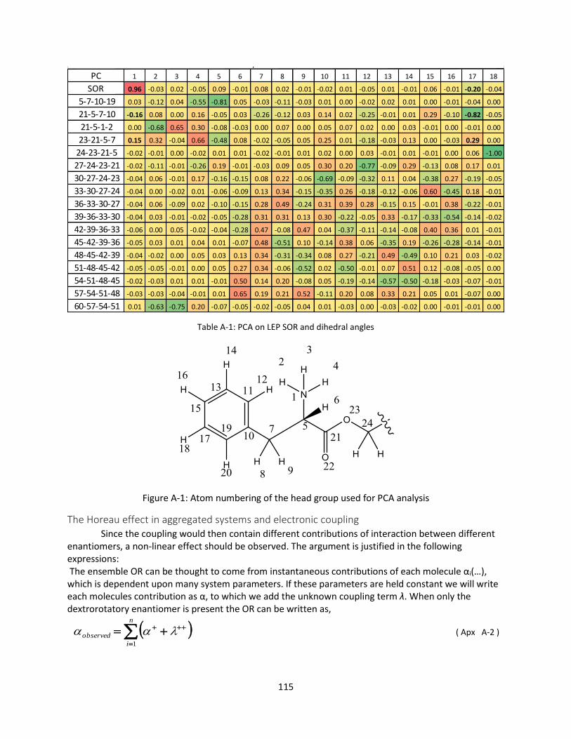
115

Table A-1: PCA on LEP SOR and dihedral angles

Figure A-1: Atom numbering of the head group used for PCA analysis

The Horeau effect in aggregated systems and electronic coupling Since the coupling would then contain different contributions of interaction between different

enantiomers, a non-linear effect should be observed. The argument is justified in the following expressions: The ensemble OR can be thought to come from instantaneous contributions of each molecule αi(…), which is dependent upon many system parameters. If these parameters are held constant we will write each molecules contribution as α, to which we add the unknown coupling term λ. When only the dextrorotatory enantiomer is present the OR can be written as,

n

i

observed

1

( Apx A-2 )

PC 1 2 3 4 5 6 7 8 9 10 11 12 13 14 15 16 17 18

SOR 0.96 -0.03 0.02 -0.05 0.09 -0.01 0.08 0.02 -0.01 -0.02 0.01 -0.05 0.01 -0.01 0.06 -0.01 -0.20 -0.04

5-7-10-19 0.03 -0.12 0.04 -0.55 -0.81 0.05 -0.03 -0.11 -0.03 0.01 0.00 -0.02 0.02 0.01 0.00 -0.01 -0.04 0.00

21-5-7-10 -0.16 0.08 0.00 0.16 -0.05 0.03 -0.26 -0.12 0.03 0.14 0.02 -0.25 -0.01 0.01 0.29 -0.10 -0.82 -0.05

21-5-1-2 0.00 -0.68 0.65 0.30 -0.08 -0.03 0.00 0.07 0.00 0.05 0.07 0.02 0.00 0.03 -0.01 0.00 -0.01 0.00

23-21-5-7 0.15 0.32 -0.04 0.66 -0.48 0.08 -0.02 -0.05 0.05 0.25 0.01 -0.18 -0.03 0.13 0.00 -0.03 0.29 0.00

24-23-21-5 -0.02 -0.01 0.00 -0.02 0.01 0.01 -0.02 -0.01 0.01 0.02 0.00 0.03 -0.01 0.01 -0.01 0.00 0.06 -1.00

27-24-23-21 -0.02 -0.11 -0.01 -0.26 0.19 -0.01 -0.03 0.09 0.05 0.30 0.20 -0.77 -0.09 0.29 -0.13 0.08 0.17 0.01

30-27-24-23 -0.04 0.06 -0.01 0.17 -0.16 -0.15 0.08 0.22 -0.06 -0.69 -0.09 -0.32 0.11 0.04 -0.38 0.27 -0.19 -0.05

33-30-27-24 -0.04 0.00 -0.02 0.01 -0.06 -0.09 0.13 0.34 -0.15 -0.35 0.26 -0.18 -0.12 -0.06 0.60 -0.45 0.18 -0.01

36-33-30-27 -0.04 0.06 -0.09 0.02 -0.10 -0.15 0.28 0.49 -0.24 0.31 0.39 0.28 -0.15 0.15 -0.01 0.38 -0.22 -0.01

39-36-33-30 -0.04 0.03 -0.01 -0.02 -0.05 -0.28 0.31 0.31 0.13 0.30 -0.22 -0.05 0.33 -0.17 -0.33 -0.54 -0.14 -0.02

42-39-36-33 -0.06 0.00 0.05 -0.02 -0.04 -0.28 0.47 -0.08 0.47 0.04 -0.37 -0.11 -0.14 -0.08 0.40 0.36 0.01 -0.01

45-42-39-36 -0.05 0.03 0.01 0.04 0.01 -0.07 0.48 -0.51 0.10 -0.14 0.38 0.06 -0.35 0.19 -0.26 -0.28 -0.14 -0.01

48-45-42-39 -0.04 -0.02 0.00 0.05 0.03 0.13 0.34 -0.31 -0.34 0.08 0.27 -0.21 0.49 -0.49 0.10 0.21 0.03 -0.02

51-48-45-42 -0.05 -0.05 -0.01 0.00 0.05 0.27 0.34 -0.06 -0.52 0.02 -0.50 -0.01 0.07 0.51 0.12 -0.08 -0.05 0.00

54-51-48-45 -0.02 -0.03 0.01 0.01 -0.01 0.50 0.14 0.20 -0.08 0.05 -0.19 -0.14 -0.57 -0.50 -0.18 -0.03 -0.07 -0.01

57-54-51-48 -0.03 -0.03 -0.04 -0.01 0.01 0.65 0.19 0.21 0.52 -0.11 0.20 0.08 0.33 0.21 0.05 0.01 -0.07 0.00

60-57-54-51 0.01 -0.63 -0.75 0.20 -0.07 -0.05 -0.02 -0.05 0.04 0.01 -0.03 0.00 -0.03 -0.02 0.00 -0.01 -0.01 0.00

Table S1: PCA analysis on LEP SOR and Dihedral values

116

Where indicates that the coupling is between two dextrorotatory LEP molecules and n is the

number of molecules in the in the light beam’s path. If one molecule of LEP is exchanged for the

opposite enantiomer the resultant OR is,

2

1

1

1

n

i

n

i

observed ( Apx A-3 )

Where the symmetry has been used. Therefore if the coupling term is significant, the SOR is

expected to change non-linearly when two opposite enantiomers are mixed. A graphical representation of this effect is shown in Figure A-2.

Figure A-2: Electronic coupling pictorially represented with (A) no effect and (B) measureable effect

Though the coupling terms do not exactly cancel, there is no guarantee that they do not approximately cancel, so therefore the Horeau effect is not yet considered a definitive test for electronic coupling and is thought of more as a qualitative assessment.

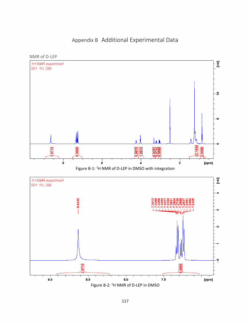
117

Appendix B Additional Experimental Data

NMR of D-LEP

Figure B-1: 1H NMR of D-LEP in DMSO with integration

Figure B-2: 1H NMR of D-LEP in DMSO

118



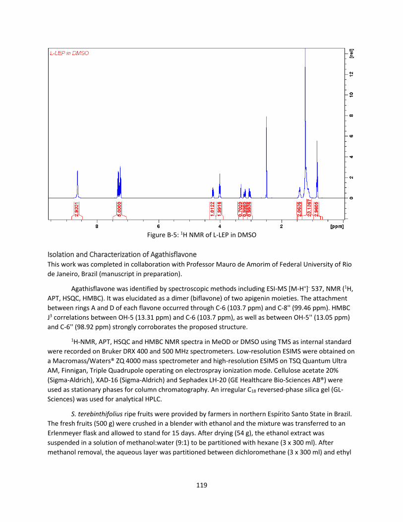
119

Figure B-5: 1H NMR of L-LEP in DMSO

Isolation and Characterization of Agathisflavone This work was completed in collaboration with Professor Mauro de Amorim of Federal University of Rio

de Janeiro, Brazil (manuscript in preparation).

Agathisflavone was identified by spectroscopic methods including ESI-MS [M-H+]- 537, NMR (1H,

APT, HSQC, HMBC). It was elucidated as a dimer (biflavone) of two apigenin moieties. The attachment

between rings A and D of each flavone occurred through C-6 (103.7 ppm) and C-8'' (99.46 ppm). HMBC

J3 correlations between OH-5 (13.31 ppm) and C-6 (103.7 ppm), as well as between OH-5'' (13.05 ppm)

and C-6'' (98.92 ppm) strongly corroborates the proposed structure.

1H-NMR, APT, HSQC and HMBC NMR spectra in MeOD or DMSO using TMS as internal standard

were recorded on Bruker DRX 400 and 500 MHz spectrometers. Low-resolution ESIMS were obtained on

a Macromass/Waters® ZQ 4000 mass spectrometer and high-resolution ESIMS on TSQ Quantum Ultra

AM, Finnigan, Triple Quadrupole operating on electrospray ionization mode. Cellulose acetate 20%

(Sigma-Aldrich), XAD-16 (Sigma-Aldrich) and Sephadex LH-20 (GE Healthcare Bio-Sciences AB®) were

used as stationary phases for column chromatography. An irregular C18 reversed-phase silica gel (GL-

Sciences) was used for analytical HPLC.

S. terebinthifolius ripe fruits were provided by farmers in northern Espírito Santo State in Brazil.

The fresh fruits (500 g) were crushed in a blender with ethanol and the mixture was transferred to an

Erlenmeyer flask and allowed to stand for 15 days. After drying (54 g), the ethanol extract was

suspended in a solution of methanol:water (9:1) to be partitioned with hexane (3 x 300 ml). After

methanol removal, the aqueous layer was partitioned between dichloromethane (3 x 300 ml) and ethyl

120

acetate (3 x 300 ml) respectively. By this procedure, hexane (6.5 g), dichloromethane (8.7 g), ethyl

acetate (11.9 g) and aqueous (20.8 g) extracts were obtained.

The ethyl acetate fraction (2.0 g) was chromatographed on a Sephadex LH-20 open column with

methanol as the mobile phase. The obtained fractions (50) were developed on a silica gel TLC plate and

sprayed with NP/PEG to search for flavonoids, which were found to occur as 23-30 fractions (yellow

spots). These fractions were pooled (440 mg) and submitted to a second Sephadex LH-20 separation,

this time with methanol:water (7:3), as the mobile phase. The flavonoid agathisflavone (20 mg) was

obtained from the fractions 38-46. ESI-MS: [M-H+]- = 537, 1H-NMR: 7.99 (2H, d, J = 0,00 Hz, H-2'/H-6'),

7.56 (2H, d, J = 0,00 Hz, H-2'''), 6.96 (2H, d, J = 0,00 Hz, H-3'/H-5'), 6.76 (2H, d, J = 0,00 Hz, H-3'''/H-5'''),

6.85 (1H, s, H-3), 6.77 (1H, s, H-3''), 6,71 (1H, s, H-8), 6.36 (1H, s, H-6''). 13C-NMR: 164.13 (C-2), 103.15

(C-3), 182.30 (C-4), 160.04 (C-5), 103.70 (C-6), 163.96 (C-7), 93.76 (C-8), 157.05 (C-9), 103.81 (C-10),

121.6 (C-1'), 128.9 (C-2'/C-6'), 116.35 (C-3'/C-5'), 161.55 (C-4'), 163.96 (C-2''), 102.90 (C-3''), 182.57 (C-

4''), 160.98 (C-5''), 98.92 (C-6''), 163.20 (C-7''), 99.46 (C-8''), not found (C-9''), 104.0 (C-10''), 121.8 (C-

1'''), 128.42 (C-2'''/C-6'''), 116.23 (C-3'''/C5'''), 161.13 (C-4''').

121

References

1. Knobloch, J.; Shaughnessy, J. D.; Rüther, U., Thalidomide induces limb deformities by perturbing the Bmp/Dkk1/Wnt signaling pathway. FASEB journal : official publication of the Federation of American Societies for Experimental Biology 2007, 21 (7), 1410-1421.

2. Friedman, L.; Miller, J. G., Odor Incongruity and Chirality. Science 1971, 172 (3987), 1044-1046.

3. Comprehensive Chiroptical Spectroscopy. Wiley: Hoboken, New Jersey, 2012; Vol. 1-2.

4. Crawford, T. D.; Tam, M. C.; Abrams, M. L., The current state of ab initio calculations of optical rotation and electronic circular dichroism spectra. J. Phys. Chem. A 2007, 111 (48), 12057-12068.

5. Kypr, J.; Kejnovska, I.; Bednarova, K.; Vorlickova, M., Circular Dichroism Spectroscopy of Nucleic Acids. Wiley: New York, 2012.

6. Kypr, J.; Kejnovská, I.; Renčiuk, D.; Vorlíčková, M., Circular dichroism and conformational polymorphism of DNA. Nucleic Acids Res. 2009, 37 (6), 1713-1725.

7. Toniolo, C.; Formaggio, F.; Woody, R. W., Electronic Circular Dichroism of Peptides. New York, 2012; Vol. 2.

8. Ma, S.; Cao, X.; Mak, M.; Sadik, A.; Walkner, C.; Freedman, T. B.; Lednev, I. K.; Dukor, R. K.; Nafie, L. A., Vibrational Circular Dichroism Shows Unusual Sensitivity to Protein Fibril Formation and Development in Solution. J. Am. Chem. Soc. 2007, 129 (41), 12364-12365.

9. Biot, J. B., Optical Activity. Mem. Institut. France, Paris 1812, 13 (1).

10. Polavarapu, P. L.; Petrovic, A.; Wang, F., Intrinsic rotation and molecular structure. Chirality 2002, 15 Suppl, 9.

11. Polavarapu, P. L., Ab initio molecular optical rotations and absolute configurations. Mol. Phys. 1997, 91 (3), 551-554.

12. Stephens, P. J.; Devlin, F. J.; Cheeseman, J. R.; Frisch, M. J., Calculation of Optical Rotation Using Density Functional Theory. J. Phys. Chem. A 2001, 105 (22), 5356-5371.

13. Autschbach, J.; Patchkovskii, S.; Ziegler, T., Chiroptical properties from time-dependent density functional theory. II. Optical rotations of small to medium sized organic molecules. J. Chem. Phys. 2002, 117 (2), 581-592.

14. Ditchfield, R., Self-consistent perturbation theory of diamagnetism. Mol. Phys. 1974, 27 (4), 789-807.

15. Autschbach, J., Computing chiroptical properties with first‐principles theoretical methods: Background and illustrative examples. Chirality 2009, 21 (1E), E116-E152.

16. Cotton, A., Absorption inegale des rayons circulaires droit et gauche dans certains corps actifs. Compt. Rend 1895, 120, 989-991.

17. Polavarapu, P. L., Renaissance in chiroptical spectroscopic methods for molecular structure determination. The Chemical Record 2007, 7 (2), 125-136.

18. Rosenfeld, L., Quantenmechanische Theorie der natürlichen optischen Aktivität von Flüssigkeiten und Gasen. Zeitschrift für Physik A Hadrons and Nuclei 1929, 52 (3-4), 161-174.

122

19. Holzwarth, G.; Hsu, E. C.; Mosher, H. S.; Faulkner, T. R.; Moscowitz, A., Infrared circular dichroism of carbon-hydrogen and carbon-deuterium stretching modes. Observations. J. Am. Chem. Soc. 1974, 96 (1), 251-252.

20. Nafie, L. A., Dual Polarization Modulation: A Real-Time, Spectral-Multiplex Separation of Circular Dichroism from Linear Birefringence Spectral Intensities. Appl. Spectrosc. 2000, 54 (11), 1634-1645.

21. biotools. http://btools.com/products.html (accessed 3/1/2016).

22. Nicu, V. P.; Baerends, E. J., Complexation, Solvation, and Chirality Transfer in Vibrational Circular Dichroism. John Wiley & sons: New York, 2012; Vol. 1.

23. Nafie, L. A., Infrared vibrational optical activity: Measurement and Instrumentation. John Wiley &sons: Hoboken, 2012; Vol. 1.

24. Stephens, P. J.; Harada, N., ECD cotton effect approximated by the Gaussian curve and other methods. Chirality 2010, 22 (2), 229-233.

25. Atkins, P. W.; Friedman, R. S., Molecular quantum mechanics. Oxford university press: 2011.

26. Becke, A. D., Density‐functional thermochemistry. III. The role of exact exchange. J. Chem. Phys. 1993, 98 (7), 5648-5652.

27. Lee, C.; Yang, W.; Parr, R. G., Development of the Colle-Salvetti correlation-energy formula into a functional of the electron density. Physical Review B 1988, 37 (2), 785-789.

28. Stephens, P. J.; McCann, D. M.; Cheeseman, J. R.; Frisch, M. J., Determination of absolute configurations of chiral molecules using ab initio time-dependent Density Functional Theory calculations of optical rotation: How reliable are absolute configurations obtained for molecules with small rotations? Chirality 2005, 17 (S1), S52-S64.

29. Crawford, T. D., Ab initio calculation of molecular chiroptical properties. Theor. Chem. Acc. 2005, 115.

30. Crawford, T. D., High-Accuracy Qunatum Chemistry and Chiroptical Properties. Wiley: New York, 2012; Vol. 1.

31. Crawford, T. D.; Allen, W. D., Optical activity in conformationally flexible molecules: a theoretical study of large-amplitude vibrational averaging in (R)-3-chloro-1-butene. Mol. Phys. 2009, 107 (8-12), 1041-1057.

32. Crawford, T. D.; Owens, L. S.; Tam, M. C.; Schreiner, P. R.; Koch, H., Ab Initio Calculation of Optical Rotation in (P)-(+)-[4]Triangulane. J. Am. Chem. Soc. 2005, 127 (5), 1368-1369.

33. Crawford, T. D.; Ruud, K., Coupled-Cluster Calculations of Vibrational Raman Optical Activity Spectra. ChemPhysChem 2011, 12 (17), 3442-3448.

34. Crawford, T. D.; Stephens, P. J., Comparison of time-dependent density-functional theory and coupled cluster theory for the calculation of the optical rotations of chiral molecules. The journal of physical chemistry. A 2008, 112 (6), 1339-1345.

35. Tsuzuki, S.; Uchimaru, T.; Tanabe, K., Conformational analysis of n-alkanes using density functional theory. Comparison with ab initio calculations. Chem. Phys. Lett. 1995, 246 (1–2), 9-12.

36. Scalmani, G.; Frisch, M. J., Continuous surface charge polarizable continuum models of solvation. I. General formalism. J. Chem. Phys. 2010, 132 (11), 114110.

http://btools.com/products.html

123

37. Mennucci, B.; Tomasi, J.; Cammi, R.; Cheeseman, J. R.; Frisch, M. J.; Devlin, F. J.; Gabriel, S.; Stephens, P. J., Polarizable Continuum Model (PCM) Calculations of Solvent Effects on Optical Rotations of Chiral Molecules. J. Phys. Chem. A 2002, 106, 6102-6113.

38. Wang, J.; Wolf, R. M.; Caldwell, J. W.; Kollman, P. A.; Case, D. A., Development and testing of a general amber force field. J. Comput. Chem. 2004, 25 (9), 1157-1174.

39. Elstner, M.; Porezag, D.; Jungnickel, G.; Elsner, J.; Haugk, M.; Frauenheim, T.; Suhai, S.; Seifert, G., Self-consistent-charge density-functional tight-binding method for simulations of complex materials properties. Physical Review B 1998, 58 (11), 7260-7268.

40. Elstner, M.; Jalkanen, K. J.; Knapp-Mohammady, M.; Frauenheim, T.; Suhai, S., Energetics and structure of glycine and alanine based model peptides: Approximate SCC-DFTB, AM1 and PM3 methods in comparison with DFT, HF and MP2 calculations. Chem. Phys. 2001, 263 (2–3), 203-219.

41. Thiel, W., Semiempirical quantum–chemical methods. Wiley Interdisciplinary Reviews: Computational Molecular Science 2014, 4 (2), 145-157.

42. Stewart, J. J. P., Optimization of parameters for semiempirical methods V: Modification of NDDO approximations and application to 70 elements. J. Mol. Model. 2007, 13 (12), 1173-1213.

43. Szabo, A.; Ostlund, N. S., Modern quantum chemistry: introduction to advanced electronic structure theory. McGraw-Hill Inc.: 1989.

44. Fatmi, M. Q.; Hofer, T. S.; Randolf, B. R.; Rode, B. M., An extended ab initio QM/MM MD approach to structure and dynamics of Zn(II) in aqueous solution. J. Chem. Phys. 2005, 123 (5), 054514.

45. Seabra, G. d. M.; Walker, R. C.; Elstner, M.; Case, D. A.; Roitberg, A. E., Implementation of the SCC-DFTB Method for Hybrid QM/MM Simulations within the Amber Molecular Dynamics Package. The Journal of Physical Chemistry A 2007, 111 (26), 5655-5664.

46. Walker, R. C.; Crowley, M. F.; Case, D. A., The implementation of a fast and accurate QM/MM potential method in Amber. J. Comput. Chem. 2008, 29 (7), 1019-1031.

47. Chen, J.; Wang, J.; Zhang, Q.; Chen, K.; Zhu, W., A comparative study of trypsin specificity based on QM/MM molecular dynamics simulation and QM/MM GBSA calculation. J. Biomol. Struct. Dyn. 2015, 33 (12), 2606-2618.

48. Kerdcharoen, T.; Morokuma, K., ONIOM-XS: an extension of the ONIOM method for molecular simulation in condensed phase. Chem. Phys. Lett. 2002, 355 (3–4), 257-262.

49. Bulo, R. E.; Ensing, B.; Sikkema, J.; Visscher, L., Toward a Practical Method for Adaptive QM/MM Simulations. Journal of Chemical Theory and Computation 2009, 5 (9), 2212-2221.

50. Park, K.; Götz, A. W.; Walker, R. C.; Paesani, F., Application of Adaptive QM/MM Methods to Molecular Dynamics Simulations of Aqueous Systems. Journal of Chemical Theory and Computation 2012, 8 (8), 2868-2877.

51. Okamoto, T.; Ishikawa, T.; Koyano, Y.; Yamamoto, N.; Kuwata, K.; Nagaoka, M., A Minimal Implementation of the AMBER-PAICS Interface for Ab Initio FMO-QM/MM-MD Simulation. Bull. Chem. Soc. Jpn. 2013, 86 (2), 210-222.

52. Kuppens, T.; Langenaeker, W.; Tollenaere, J. P.; Bultinck, P., Determination of the Stereochemistry of 3-Hydroxymethyl-2,3-dihydro-[1,4]dioxino[2,3-b]- pyridine by Vibrational Circular Dichroism and the Effect of DFT Integration Grids. The Journal of Physical Chemistry A 2003, 107 (4), 542-553.

124

53. Debie, E.; De Gussem, E.; Dukor, R. K.; Herrebout, W.; Nafie, L. A.; Bultinck, P., A Confidence Level Algorithm for the Determination of Absolute Configuration Using Vibrational Circular Dichroism or Raman Optical Activity. ChemPhysChem 2011, 12 (8), 1542-1549.

54. Shen, J.; Zhu, C.; Reiling, S.; Vaz, R., A novel computational method for comparing vibrational circular dichroism spectra. Spectrochim. Acta Mol. Biomol. Spectros. 2010, 76 (3–4), 418–422.

55. Polavarapu, P. L.; Covington, C. L., Comparison of Experimental and Calculated Chiroptical Spectra for Chiral Molecular Structure Determination. Chirality 2014, 26 (9), 539-552.

56. Polavarapu, P. L.; Covington, C. L., Wavelength resolved specific optical rotations and homochiral equilibria. PCCP 2015, 17, 21630-21633.

57. Covington, C. L.; Polavarapu, P. L., Specific optical rotations and the Horeau effect. Chirality 2015.

58. Nakao, Y.; Sugeta, H.; Kyogoku, Y., Intermolecular Hydrogen Bonding of Enantiomers of Pantolactone Studied by Infrared and <SUP>1</SUP>H-NMR Spectroscopy. Bull. Chem. Soc. Jpn. 1985, 58 (6), 1767-1771.

59. Baciocchi, R.; Zenoni, G.; Valentini, M.; Mazzotti, M.; Morbidelli, M., Measurement of the Dimerization Equilibrium Constants of Enantiomers. J. Phys. Cem. A 2002, 106 (43), 10461-10469.

60. Goldsmith, M.-R.; Jayasuriya, N.; Beratan, D. N.; Wipf, P., Optical Rotation of Noncovalent Aggregates. J. Am. Chem. Soc. 2003, 125 (51), 15696-15697.

61. Tellinghuisen, J., Nonlinear Least-Squares Using Microcomputer Data Analysis Programs: KaleidaGraph™ in the Physical Chemistry Teaching Laboratory. J. Chem. Educ. 2000, 77 (9), 1233.

62. Yan, Z.; Donald, G. T., The M06 suite of density functionals for main group thermochemistry, thermochemical kinetics, noncovalent interactions, excited states, and transition elements: two new functionals and systematic testing of four M06-class functionals and 12 other functionals. Theor. Chem. Acc. 2007, 120.

63. McCann, D. M.; Stephens, P. J., Determination of Absolute Configuration Using Density Functional Theory Calculations of Optical Rotation and Electronic Circular Dichroism: Chiral Alkenes. The Journal of Organic Chemistry 2006, 71 (16), 6074-6098.

64. Ruud, K.; Taylor, P. R.; Åstrand, P.-O., Zero-point vibrational effects on optical rotation. Chem. Phys. Lett. 2001, 337 (1–3), 217-223.

65. Wiberg, K. B.; Vaccaro, P. H.; Cheeseman, J. R., Conformational Effects on Optical Rotation. 3-Substituted 1-Butenes. J. Am. Chem. Soc. 2003, 125 (7), 1888-1896.

66. Mort, B. C.; Autschbach, J., Temperature Dependence of the Optical Rotation of Fenchone Calculated by Vibrational Averaging. The Journal of Physical Chemistry A 2006, 110 (40), 11381-11383.

67. Horeau, A., Interactions d'enantiomeres en solution ; influence sur le pouvoir rotatoire : Purete optique et purete enantiomerique. Tetrahedron Lett. 1969, 10 (36), 3121-3124.

68. Horeau, A.; Guetté, J. P., Interactions diastereoisomeres d'antipodes en phase liquide. Tetrahedron 1974, 30 (13), 1923-1931.

69. Solladié-Cavallo, A.; Andriamiadanarivo, R., Hydroxypinanone: Solute/solute interactions and non-linear chiroptical properties. Tetrahedron Lett. 1997, 38 (33), 5851-5852.

70. Acs, M., Chiral recognition in the light of molecular associations Akademiai Kiado: Budapest, 1990.

125

71. Eliel, E. L.; Wilen, S. H., Stereochemistry of Organic Compounds. John Wiley: New York, 1994.

72. Eliel, E. L.; Wilen, S. H.; Doyle, M. P., Basic Organic Stereochemistry. Wiley: 2001.

73. MacroModel MacroModel, Schrödinger, LLC: New York, NY, 2015.

74. Rosen, M. J., Surfactants and Interfacial Phenomena. John Wiley & Sons: New York, 1978.

75. Moroi, Y., Micelles: Theoretical and Applied Aspects. Plenum Press: New York, 1992.

76. Myers, D., Surfaces, Interfaces, and Colloids: Principles and Applications. Wiley: New York, NY, 1999; Vol. 2.

77. Polavarapu, P. L.; Vijay, R., Chiroptical Spectroscopy of Surfactants. J. Phys. Chem. A 2012.

78. Vijay, R.; Polavarapu, P. L., FMOC-amino acid surfactants: discovery, characterization and chiroptical spectroscopy. J. Phys. Chem. A 2012, 116 (44), 10759-10769.

79. Vijay, R.; Baskar, G.; Mandal, A. B.; Polavarapu, P. L., Unprecedented Relationship Between the Size of Spherical Chiral Micellar Aggregates and Their Specific Optical Rotations. J. Phys. Chem. A 2013, 117 (18), 3791-3797.

80. Vijay, R.; Angayarkanny, S.; Geetha, B., Amphiphilic dodecyl ester derivatives from aromatic amino acids: Significance of chemical architecture in interfacial adsorption characteristics. Colloids Surf., A 2008, 317 (3), 643-649.

81. Vijay, R.; Mandal, A. B.; Baskar, G., 1H NMR Spectroscopic Investigations on the Conformation of Amphiphilic Aromatic Amino Acid Derivatives in Solution: Effect of Chemical Architecture of Amphiphiles and Polarity of Solvent Medium. The Journal of Physical Chemistry B 2010, 114 (43), 13691-13702.

82. Brizard, A.; Berthier, D.; Aimé, C.; Buffeteau, T.; Cavagnat, D.; Ducasse, L.; Huc, I.; Oda, R., Molecular and supramolecular chirality in gemini-tartrate amphiphiles studied by electronic and vibrational circular dichroisms. Chirality 2009, 21 (1E), E153-E162.

83. Schenning, A.; Kilbinger, A. F. M.; Biscarini, F., Supramolecular organization of α, α'-disubstituted sexithiophenes. J. Am. Chem. Soc. 2002, 124 (7), 1269-1275.

84. Goerigk, L.; Grimme, S., Quantum Chemical Investigation of Exciton Coupling: Super‐Molecular Calculations of a Merocyanine Dimer Aggregate. ChemPhysChem 2008.

85. Pescitelli, G.; Padula, D.; Santoro, F., Intermolecular exciton coupling and vibronic effects in solid-state circular dichroism: a case study. Phys. Chem. Chem. Phys. 2012, 15 (3), 795-802.

86. Schweitzer-Stenner, R., Internal electric field in cytochrome C explored by visible electronic circular dichroism spectroscopy. J. Phys. Chem. B 2008, 112, 10358–10366.

87. Polavarapu, P. L., Kramers−Kronig Transformation for Optical Rotatory Dispersion Studies. The Journal of Physical Chemistry A 2005, 109 (32), 7013-7023.

88. Marrink, S. J.; Tieleman, D. P.; Mark, A. E., Molecular Dynamics Simulation of the Kinetics of Spontaneous Micelle Formation. J. Phys. Chem. B 2000, 104 (51), 12165-12173.

89. Sammalkorpi, M.; Karttunen, M.; Haataja, M., Structural Properties of Ionic Detergent Aggregates: A Large-Scale Molecular Dynamics Study of Sodium Dodecyl Sulfate. J. Phys. Chem. B 2007, 111 (40), 11722-11733.

126

90. Prabal, K. M.; Yves, L.; Matthew, A. G.; Noel, A. C.; Yannick, R., Self-Assembly in Surfactant Oligomers: A Coarse-Grained Description through Molecular Dynamics Simulations. Langmuir 2002, 18.

91. Kirkwood, J. G., On the Theory of Optical Rotatory Power. J. Chem. Phys. 1937, 5 (6).

92. Applequist, J., On the polarizability theory of optical rotation. J. Chem. Phys 1973, 58 (10), 4251-4259.

93. Applequist, J., An atom dipole interaction model for molecular optical properties. Acc. Chem. Res. 1977.

94. Zhang, G.; Musgrave, C. B., Comparison of DFT methods for molecular orbital eigenvalue calculations. J. Phys. Chem. A 2007, 111 (8), 1554-1561.

95. Martínez, L.; Andrade, R.; Birgin, E. G.; Martínez, J. M., PACKMOL: A package for building initial configurations for molecular dynamics simulations. J. Comput. Chem 2009, 30 (13), 2157-2164.

96. Callum, J. D.; Lula, R.; Robin, M. B.; Ross, C. W.; Ian, R. G., GAFFlipid: a General Amber Force Field for the accurate molecular dynamics simulation of phospholipid. Soft Matter 2012, 8.

97. Jorgensen, W. L.; Chandrasekhar, J.; Madura, J. D.; Impey, R. W.; Klein, M. L., Comparison of simple potential functions for simulating liquid water. J. Chem. Phys. 1983, 79 (2), 926-935.

98. Mao, Y.; Zhang, Y., Thermal conductivity, shear viscosity and specific heat of rigid water models. Chem. Phys. Lett. 2012, 542, 37-41.

99. Betz, R. M.; Walker, R. C., Paramfit: Automated optimization of force field parameters for molecular dynamics simulations. J. Comput. Chem. 2015, 36 (2), 79-87.

100. Dupradeau, F.-Y. Y.; Pigache, A.; Zaffran, T.; Savineau, C.; Lelong, R.; Grivel, N.; Lelong, D.; Rosanski, W.; Cieplak, P., The R.E.D. tools: advances in RESP and ESP charge derivation and force field library building. Phys. Chem. Chem. Phys. 2010, 12 (28), 7821-7839.

101. D.A. Case, T. A. D., T.E. Cheatham, III, C.L. Simmerling, J. Wang, R.E. Duke, R. Luo, R.C. Walker, W. Zhang, K.M. Merz, B. Roberts, S. Hayik, A. Roitberg, G. Seabra, J. Swails, A.W. Goetz, I. Kolossváry, K.F. Wong, F. Paesani, J. Vanicek, R.M. Wolf, J. Liu, X. Wu, S.R. Brozell, T. Steinbrecher, H. Gohlke, Q. Cai, X. Ye, J. Wang, M.-J. Hsieh, G. Cui, D.R. Roe, D.H. Mathews, M.G. Seetin, R. Salomon-Ferrer, C. Sagui, V. Babin, T. Luchko, S. Gusarov, A. Kovalenko, and P.A. Kollman AMBER 12, University of California: San Francisco, 2012.

102. Ryckaert, J.-P.; Ciccotti, G.; Berendsen, H. J. C., Numerical integration of the cartesian equations of motion of a system with constraints: molecular dynamics of n-alkanes. Journal of Computational Physics 1977, 23 (3), 327-341.

103. Case, D. A.; Berryman, J. T.; Betz, R. M.; Cerutti, T. E.; Cheatham, T. E. I.; Darden, T.; Duke, R. E.; Giese, T. J.; Gohlke, H.; Goetz, A. W.; Homeyer, N.; Izadi, S.; Janowski, P.; Kaus, J.; Kovalenko, A.; Lee, T. S.; LeGrand, S.; Li, P.; Luchko, T.; Luo, R.; Madej, B. D.; Merz, K. M.; Monard, G.; Needham, P.; Nguyen, H.; Nguyen, H. T.; Omelyan, I.; Onufriev, A.; Roe, D. R.; Roitberg, A.; Salomon-Ferrer, R.; Simmerling, C. L.; Smith, W.; Swails, J.; Walker, R. C.; Wang, J.; Wolf, R. M.; Wu, X.; York, D.; Kollman, P. A. AMBER 2015, University of California, San Francisco., 2015.

104. Takenaka, N.; Kitamura, Y.; Koyano, Y.; Nagaoka, M., An improvement in quantum mechanical description of solute-solvent interactions in condensed systems via the number-adaptive multiscale quantum mechanical/molecular mechanical-molecular dynamics method: Application to zwitterionic glycine in aqueous solution. J. Chem. Phys. 2012, 137 (2), 024501.

127

105. Roe, D. R.; Cheatham, T. E. I., PTRAJ and CPPTRAJ: software for processing and analysis of molecular dynamics trajectory data. J. Chem. Theory Comput. 2013, 9, 3084−3095.

106. Humphrey, W.; Dalke, A.; Schulten, K., VMD: Visual molecular dynamics. Journal of Molecular Graphics 1996, 14 (1), 33-38.

107. Hanwell, M. D.; Curtis, D. E.; Lonie, D. C.; Vandermeersch, T.; Zurek, E.; Hutchison, G. R., Avogadro: an advanced semantic chemical editor, visualization, and analysis platform. Journal of Cheminformatics 2012, 4, 17-17.

108. Frisch, M. J.; Trucks, G. W.; Schlegel, H. B.; Scuseria, G. E.; Robb, M. A.; Cheeseman, J. R.; Scalmani, G.; Barone, V.; Mennucci, B.; Petersson, G. A.; Nakatsuji, H.; Caricato, M.; Li, X.; Hratchian, H. P.; Izmaylov, A. F.; Bloino, J.; Zheng, G.; Sonnenberg, J. L.; Hada, M.; Ehara, M.; Toyota, K.; Fukuda, R.; Hasegawa, J.; Ishida, M.; Nakajima, T.; Honda, Y.; Kitao, O.; Nakai, H.; Vreven, T.; Montgomery, J., J. A.; Peralta, J. E.; Ogliaro, F.; Bearpark, M.; Heyd, J. J.; Brothers, E.; Kudin, K. N.; Staroverov, V. N.; Kobayashi, R.; Normand, J.; Raghavachari, K.; Rendell, A.; Burant, J. C.; Iyengar, S. S.; Tomasi, J.; Cossi, M.; Rega, N.; Millam, J. M.; Klene, M.; Knox, J. E.; Cross, J. B.; Bakken, V.; Adamo, C.; Jaramillo, J.; Gomperts, R.; Stratmann, R. E.; Yazyev, O.; Austin, A. J.; Cammi, R.; Pomelli, C.; Ochterski, J. W.; Martin, R. L.; Morokuma, K.; Zakrzewski, V. G.; Voth, G. A.; Salvador, P.; Dannenberg, J. J.; Dapprich, S.; Daniels, A. D.; Farkas, Ö.; Foresman, J. B.; Ortiz, J. V.; Cioslowski, J.; Fox, D. J. Gaussian 09, Gaussian Inc.: Wallingford CT, 2009.

109. Aidas, K.; Angeli, C.; Bak, K. L.; Bakken, V.; Bast, R.; Boman, L.; Christiansen, O.; Cimiraglia, R.; Coriani, S.; Dahle, P.; Dalskov, E. K.; Ekström, U.; Enevoldsen, T.; Eriksen, J. J.; Ettenhuber, P.; Fernández, B.; Ferrighi, L.; Fliegl, H.; Frediani, L.; Hald, K.; Halkier, A.; Hättig, C.; Heiberg, H.; Helgaker, T.; Hennum, A. C.; Hettema, H.; Hjertenæs, E.; Høst, S.; Høyvik, I.-M.; Iozzi, M. F.; Jansík, B.; Jensen, H. J. A.; Jonsson, D.; Jørgensen, P.; Kauczor, J.; Kirpekar, S.; Kjærgaard, T.; Klopper, W.; Knecht, S.; Kobayashi, R.; Koch, H.; Kongsted, J.; Krapp, A.; Kristensen, K.; Ligabue, A.; Lutnæs, O. B.; Melo, J. I.; Mikkelsen, K. V.; Myhre, R. H.; Neiss, C.; Nielsen, C. B.; Norman, P.; Olsen, J.; Olsen, J. M. H.; Osted, A.; Packer, M. J.; Pawlowski, F.; Pedersen, T. B.; Provasi, P. F.; Reine, S.; Rinkevicius, Z.; Ruden, T. A.; Ruud, K.; Rybkin, V. V.; Sałek, P.; Samson, C. C. M.; de Merás, A. S.; Saue, T.; Sauer, S. P. A.; Schimmelpfennig, B.; Sneskov, K.; Steindal, A. H.; Sylvester-Hvid, K. O.; Taylor, P. R.; Teale, A. M.; Tellgren, E. I.; Tew, D. P.; Thorvaldsen, A. J.; Thøgersen, L.; Vahtras, O.; Watson, M. A.; Wilson, D. J. D.; Ziolkowski, M.; Ågren, H., The Dalton quantum chemistry program system. Wiley Interdisciplinary Reviews: Computational Molecular Science 2014, 4 (3), 269-284.

110. Flyvbjerg , H.; Petersen, H. G., Error estimates on averages of correlated data. J. Chem. Phys.: 1989; Vol. 91, p 461.

111. Sanderson, C. Armadillo: An open source C++ linear algebra library for fast prototyping and computationally intensive experiments. http://arma.sourceforge.net/ (accessed 2/29/2016).

112. Covington, C. L.; Polavarapu, P. L., Similarity in Dissymmetry Factor Spectra: A Quantitative Measure of Comparison between Experimental and Predicted Vibrational Circular Dichroism. J. Phys. Cem. A 2013, 117 (16), 3377-3386.

113. Debie, E.; Bultinck, P.; Herrebout, W.; van der Veken, B., Solvent effects on IR and VCD spectra of natural products: an experimental and theoretical VCD study of pulegone. Phys. Chem. Chem. Phys. 2008, 10 (24), 3498-508.

114. Nicu, V. P.; Baerends, E. J., Robust normal modes in vibrational circular dichroism spectra. Phys. Chem. Chem. Phys. 2009, 11 (29), 6107-18.

http://arma.sourceforge.net/

128

115. Gobi, S.; Magyarfalvi, G., Reliability of computed signs and intensities for vibrational circular dichroism spectra. Phys. Chem. Chem. Phys. 2011, 13 (36), 16130-3.

116. Barron, L. D., Molecular Light Scattering and Optical Activity. Cambridge Univ Press: Cambridge, 2004.

117. Kuhn, W., The physical significance of optical rotatory power. Trans. Faraday Soc. 1930, 26 (0), 293-308.

118. He, J.; Petrovic, A. G.; Polavarapu, P. L., Determining the Conformer Populations of (R)-(+)-3-Methylcyclopentanone Using Vibrational Absorption, Vibrational Circular Dichroism, and Specific Rotation. J. Phys. Chem. B, 2004, 108 (52), 20451-20457.

119. He, J.; Petrovich, A.; Polavarapu, P. L., Quantitative Determination of Conformer Populations: Assessment of Specific Rotation, Vibrational Absorption, and Vibrational Circular Dichroism in Substituted Butynes. J. Phys. Cem. A 2004, 108 (10), 1671-1680.

120. Wang, F.; Polavarapu, P., L, Conformational Stability of (+)-Epichlorohydrin. J. Phys. Chem. A 2000, 104 (26), 6189-6196.

121. Longhi, G.; Abbate, S.; Gangemi, R.; Giorgio, E.; Rosini, C., Fenchone, Camphor, 2-Methylenefenchone and 2-Methylenecamphor: A Vibrational Circular Dichroism Study. J. Phys. Chem. A, 2006, 110 (15), 4958-4968.

122. Polavarapu, P. L.; Petrovic, A. G.; Vick, S. E.; Wulff, W. D.; Ren, H.; Ding, Z.; Staples, R. J., Absolute

Configuration of 3,3′-Diphenyl-[2,2′-binaphthalene]-1,1′-diol Revisited. The Journal of Organic Chemistry 2009, 74 (15), 5451-5457.

123. Vandenbussche, J.; Bultinck, P.; Przybył, A. K.; Herrebout, W. A., Statistical validation of absolute configuration assignment in vibrational optical activity. J. Chem. Theory. Comput. 2013, 9, 5504-5512.

124. Conflex Conflex: High Performance Conformational Analysis, http://www.conflex.us/: May 24, 2010.

125. Junior, F. M. S.; Covington, C. L.; de Albuquerque, A. C. F.; Lobo, J. F. R.; Borges, R. M.; de Amorim, M. B.; Polavarapu, P. L., Absolute Configuration of (−)-Centratherin, a Sesquiterpenoid Lactone, Defined by Means of Chiroptical Spectroscopy. J. Nat. Prod. 2015, 78 (11), 2617-2623.

126. Bijvoet, J. M.; Peerdeman, A. F.; van Bommel, A. J., Determination of the Absolute Configuration of Optically Active Compounds by Means of X-Rays. Nature 1951, 168 (4268), 271-272.

127. Flack, H. D.; Bernardinelli, G., The use of X-ray crystallography to determine absolute configuration. Chirality 2008, 20 (5), 681-690.

128. Picman, A. K., Biological activities of sesquiterpene lactones. Biochem. Syst. Ecol. 1986, 14 (3), 255-281.

129. Rüngeler, P.; Castro, V.; Mora, G.; Gören, N.; Vichnewski, W.; Pahl, H. L.; Merfort, I.; Schmidt, T. J., Inhibition of transcription factor NF-κB by sesquiterpene lactones: a proposed molecular mechanism of action. Biorg. Med. Chem. 1999, 7 (11), 2343-2352.

130. Burim, R. V.; Canalle, R.; Lopes, J. L. C.; Vichnewski, W.; Takahashi, C. S., Genotoxic action of the sesquiterpene lactone centratherin on mammalian cells in vitro and in vivo. Teratogenesis, Carcinogenesis, and Mutagenesis 2001, 21 (6), 383-393.

http://www.conflex.us/:

129

131. Bohlmann, F.; Zdero, C.; Robinson, H.; King, R. M., Caryophyllene derivatives and a heliangolide from Lychnophora species. Phytochemistry 1980, 19 (11), 2381-2385.

132. Le Quesne, P. W.; Menachery, M. D.; Pastore, M. P.; Kelley, C. J.; Brennan, T. F.; Onan, K. D.; Raffauf, R. F.; Weeks, C. M., Antitumor plants. 12. Further sesquiterpenoid constituents of Lychnophora affinis Gardn. (Compositae). X-ray structure analysis of lychnophorolide A. The Journal of Organic Chemistry 1982, 47 (8), 1519-1521.

133. Halgren, T. A., MMFF VI. MMFF94s option for energy minimization studies. J. Comput. Chem. 1999, 20 (7), 720-729.

134. Mennucci, B.; Cappelli, C.; Cammi, R.; Tomasi, J., Modeling solvent effects on chiroptical properties. Chirality 2011, 23 (9), 717-729.

135. Junior, F. M. S.; Covington, C. L.; de Amorim, M. B.; Velozo, L. S. M.; Kaplan, M. A. C.; Polavarapu, P. L., Absolute Configuration of a Rare Sesquiterpene: (+)-3-Ishwarone. J. Nat. Prod. 2014, 77 (8), 1881-1886.

136. Polavarapu, P. L.; Donahue, E. A.; Shanmugam, G.; Scalmani, G.; Hawkins, E. K.; Rizzo, C.; Ibnusaud, I.; Thomas, G.; Habel, D.; Sebastian, D., A Single Chiroptical Spectroscopic Method May Not Be Able To Establish the Absolute Configurations of Diastereomers: Dimethylesters of Hibiscus and Garcinia Acids. J. Phys. Chem. A 2011, 115 (22), 5665-5673.

137. Li, X.-C.; Ferreira, D.; Ding, Y., Determination of Absolute Configuration of Natural Products: Theoretical Calculation of Electronic Circular Dichroism as a Tool. Curr. Org. Chem. 2010, 14, 1678-1697.

138. Polavarapu, P. L., Why is it important to simultaneously use more than one chiroptical spectroscopic method for determining the structures of chiral molecules? Chirality 2008, 20 (5), 664-672.

139. Junior, F. M.; Velozo, L. S.; de Carvalho, E. M.; Marques, A. M.; Borges, R. M.; Trindade, A. P.; dos Santos, M. I.; de Albuquerque, A. C.; Costa, F. L.; Kaplan, M. A.; de Amorim, M. B., 3-Ishwarone, a rare ishwarane sesquiterpene from Peperomia scandens Ruiz & Pavon: structural elucidation through a joint experimental and theoretical study. Molecules (Basel, Switzerland) 2012, 18 (11), 13520-13529.

140. Lago, J. H. G.; Oliveira, A. d.; Guimarães, E. F.; Kato, M. J., 3-Ishwarone and 3-Ishwarol, rare sesquiterpenes in essential oil from leaves of Peperomia oreophila Hensch. Journal of the Brazilian Chemical Society 2007, 18, 638-642.

141. Derewacz, D. K.; McNees, C. R.; Scalmani, G.; Covington, C. L.; Shanmugam, G.; Marnett, L. J.; Polavarapu, P. L.; Bachmann, B. O., Structure and Stereochemical Determination of Hypogeamicins from a Cave-Derived Actinomycete. J. Nat. Prod. 2014, 77 (8), 1759-1763.

142. Berdy, J., Bioactive Microbial Metabolites. J. Antibiot. 2005, 58 (1), 1-26.

143. Harborne, J. B., The flavonoids.Advances in research science 1980. Chapman and Hall: New York, 1988; p 621.

144. Ilyas, M.; Usmani, J. N.; Bhatnagar, S. P.; Ilyas, M.; Rahman, W., WB1 and W11, the first optically active biflavones. Tetrahedron Lett. 1968, 9 (53), 5515-5517.

145. Bringmann, G.; Günther, C.; Ochse, M.; Schupp, O.; Tasler, S., Progress in the Chemistry of Organic Natural Products. Herz, W.; Falk, H.; Kirby, G. W.; Moore, R. E., Eds. Springer: Vienna, 2001; Vol. 82, pp 74-88.

130

146. Baba, K.; Tabata, Y.; Taniguti, M.; Kozawa, M., Coumarins from Edgeworthia chrysantha. Phytochemistry 1989, 28 (1), 221-225.

147. Harada, N.; Ono, H.; Uda, H.; Parveen, M.; Khan Nizam ud, D.; Achari, B.; Dutta, P. K., Atropisomerism in natural products. Absolute stereochemistry of biflavone, (-)-4',4''',7,7''-tetra-O-methylcupressuflavone, as determined by the theoretical calculation of CD spectra. J. Am. Chem. Soc. 1992, 114 (20), 7687-7692.

148. Barbosa, L. C. A.; Demuner, A. J.; Clemente, A. D.; Paula, V. F. d.; Ismail, F. M. D., Seasonal variation in the composition of volatile oils from Schinus terebinthifolius raddi. Quim. Nova 2007, 30, 1959-1965.

149. Losada, M.; Xu, Y., Chirality transfer through hydrogen-bonding: Experimental and ab initio analyses of vibrational circular dichroism spectra of methyl lactate in water. PCCP 2007, 9 (24), 3127-3135.

150. Losada, M.; Nguyen, P.; Xu, Y., Solvation of Propylene Oxide in Water: Vibrational Circular Dichroism, Optical Rotation, and Computer Simulation Studies. The Journal of Physical Chemistry A 2008, 112 (25), 5621-5627.

151. Losada, M.; Tran, H.; Xu, Y., Lactic acid in solution: Investigations of lactic acid self-aggregation and hydrogen bonding interactions with water and methanol using vibrational absorption and vibrational circular dichroism spectroscopies. J. Chem. Phys. 2008, 128 (1), -.

152. Wang, J.; Wang, W.; Kollman, P. A.; Case, D. A., Automatic atom type and bond type perception in molecular mechanical calculations. J. Mol. Graphics Modell. 2006, 25 (2), 247–260.

153. Jakalian, A.; Bush, B. L.; Jack, D. B.; Bayly, C. I., Fast, efficient generation of high-quality atomic charges. AM1-BCC model: I. Method. J. Comput. Chem. 2000, 21 (2), 132-146.

154. Jakalian, A.; Jack, D. B.; Bayly, C. I., Fast, efficient generation of high-quality atomic charges. AM1-BCC model: II. Parameterization and validation. J. Comput. Chem. 2002, 23 (16), 1623-1641.

155. Miyamoto, S.; Kollman, P. A., Settle: An analytical version of the SHAKE and RATTLE algorithm for rigid water models. J. Comput. Chem. 1992, 13 (8), 952-962.

156. Covington, C. L.; Nicu, V. P.; Polavarapu, P. L., Determination of Absolute Configurations Using Exciton Chirality Method for Vibrational Circular Dichroism: Right Answers for the Wrong Reasons ?? J. Phys. Chem. 2015, 119, 10589−10601

157. Tinoco, I., Jr., The Exciton Contribution to the Optical Rotation of Polymers. Radiat. Res. 1963, 20, 133-139.

158. Tinoco, I., Jr.; Cantor, C. R., Application of Optical Rotatory Dispersion and Circular Dichroism in Biochemical Analysis. John Wiley & Sons: New york, 1970; Vol. 18.

159. Harada, N.; Nakanishi, K., Circular Dichroic Spectroscopy. Exciton Coupling in Organic Stereochemistry. Univ. Sci. Books: 1983; p 460 pp.

160. Rodger, A.; Norden, B., Circular Dichroism and Linear Dichroism. Oxford University Press: Oxford, 1997.

161. Berova, N.; Bari, L. D.; Pescitelli, G., Application of electronic circular dichroism in configurational and conformational analysis of organic compounds. Chem. Soc. Rev. 2007, 36 (6), 914-931.

131

162. Bruhn, T.; Pescitelli, G.; Jurinovich, S.; Schaumlöffel, A.; Witterauf, F.; Ahrens, J.; Bröring, M.; Bringmann, G., Axially Chiral BODIPY DYEmers: An Apparent Exception to the Exciton Chirality Rule. Angew. Chem. Int. Ed. 2014, 53, 14592-14595.

163. Holzwarth, G.; Chabay, I., Optical Activity of Vibrational Transitions: A Coupled Oscillator Model. J. Chem. Phys. 1972, 57, 1632-1635.

164. Su, C. N.; Keiderling, T. A., Conformation of Dimethyl Tartrate in Solution. Vibrational Circular Dichroism Results. J. Am. Chem. Soc. 1980, 102, 511-515.

165. Bour, P.; Keiderling, T. A., Computational Evaluation of the Coupled Oscillator Model in the Vibrational Circular Dichroism of Selected Small Molecules. J. Am. Chem. Soc. 1992, 114, 9100-9105.

166. Birke, S. S.; Agbaje, I.; Diem, M., Experimental and Computational Infrared CD Studies of Prototypical Peptide Conformations. Biochemistry 1992, 31, 450-455.

167. Buckingham, A. D.; Fowler, P. W.; Galwas, P. A., Velocity-Dependent Property Surfaces and the Theory of Vibrational Circular Dichroism. Chem. Phys. 1987, 112, 1-14.

168. Stephens, P. J., Theory of Vibrational Circular Dichroism. J. Phys. Chem. 1985, 89, 748-752.

169. Asai, T.; Taniguchi, T.; Yamamoto, T.; Monde, K.; Oshima, Y., Structures of Spiroindicumides A and B, Unprecedented Carbon Skeletal Spirolactones, and Determination of the Absolute Configuration by Vibrational Circular Dichroism Exciton Approach. Org. Lett. 2013, 15, 4320-4323.

170. Komori, K.; Taniguchi, T.; Mizutani, S.; Monde, K.; Kuramochi, K.; Tsubaki, K., Short Synthesis of Berkeleyamide D and Determination of the Absolute Configuration by the Vibrational Circular Dichroism Exciton Chirality Method. Org. Lett. 2014, 16, 1386-1389.

171. Taniguchi, T.; Monde, K., Exciton Chirality Method in Vibrational Circular Dichroism. J. Am. Chem. Soc. 2012, 134, 3695-3698.

172. Wilson, E. B.; Decius, J. C.; Cross, P. C., Molecular Vibrations: The Theory of Infrared and Raman Vibrational Spectra. Dover Publications: 1980.

173. Rohatgi, A. WebPlotDigitizer. http://arohatgi.info/WebPlotDigitizer (accessed March, 2015).

174. Abbate, S.; Mazzeo, G.; Meneghini, S.; Longhi, G.; Boiadjiev, S. E.; Lightner, D. A., Bicamphor: A Prototypic Molecular System to Investigate Vibrational Excitons. J. Phys. Chem. A 2015, 119, 4261-4267.

175. Becker, O. M.; MacKerell, A. D. J.; Roux, B.; Watanabe, M., Computational Biochemistry and Biophysics. Marcel Dekker Inc.: New York, 2001.

http://arohatgi.info/WebPlotDigitizer

chiroptical spectroscopic studies on surfactants, other...

Documents