china’s firm-level processing trade: trends,
TRANSCRIPT

1
No. E2012002 2012-04
China’s Firm-Level Processing Trade: Trends,
Characteristics, and Productivity1
Miaojie Yu2 and Wei Tian3
No. E2012002 April 10, 2012
Abstract
This paper provides a comprehensive overview of China’s processing trade using highly disaggregated 2010 transaction-level data. By highlighting the key role of processing trade in China’s foreign trade, we argue that various free-trade zones have served as important instruments in boosting processing trade. We then explore various characteristics of processing imports from both industry-level and firm-level perspectives: origin countries of imports, main products, transport modes, entry ports, consumption destinations, quality of commodities, and scope of processing trade. A careful estimation of firm-level total factor productivity using the Olley–Pakes approach suggests that processing firms are less productive than non-processing firms. We also contribute to the literature by offering an efficient way of matching firm-level production data with transaction-level trade data, a rather challenging task due to data format restrictions.
Keywords: Processing Trade, Export Processing Zones, Quality of Products, Firm Scope, Total Factor Productivity, Transaction-Level Trade Data, Firm-Level Evidence
JEL Code: F1, L1, O1
1 This paper is prepared for the conference of China’s updates (2012) organized by Australian National University in Canberra in July 2012. We thank Dr. Ligang Song for his invitation and helpful comments. Miaojie Yu thanks Yaqi Wang for her excellent research assistance. All errors are ours. 2 Corresponding Author, China Center for Economic Research, National School of Development, Peking University, Beijing ,100871, China. Tel: (+86)10‐6275‐3109; Email: [email protected] . 3 Department of Applied Economics, Guanghua School of Management, Peking University, Email: [email protected] .

2
1. Introduction
Popular in China, processing trade involves domestic firms obtaining raw materials or
intermediate inputs from abroad, processing them locally, and exporting the value-added goods.
Governments usually offer tariff reduction or tariff exemption to encourage the development of
processing trade. The current paper aims to provide a comprehensive review of various trends,
characteristics, and productivity levels of processing trade as opposed to ordinary trade in China.
We begin with an overview of processing trade, focusing on its size and main types. Thereafter,
we analyze why processing trade has developed rapidly in China in the last three decades. China’s
open-door policy, particularly the establishment of special export zones, has played a significant
role in the rapid growth of processing trade. We use transaction-level trade data (2000–2006) from
China to investigate various factors affecting processing trade, such as origin and destination
countries, leading import and export commodities, transport modes, firm ownership, leading ports
and their trade volume, and top cities and provinces where producers and consumers are located.
Our transaction-level trade data set includes firm-level information. Each trade transaction is
attributable to a particular firm. We investigate the number of products (i.e., scope) imported and
exported by firms, as well as their number of trading destinations. More importantly, because firm
productivity is key to understanding trade performance (Melitz, 2003), we investigate the
productivity growth of firms by matching transaction-level trade data with firm-level production
data, and using the Olley–Pakes (1996) semi-parametric approach for estimating firm productivity.
Furthermore, in carefully scrutinizing processing trade in China, the present paper contributes to
the literature by providing a novel and orderly way of matching two powerful data sets
(transaction-level trade data and firm-level production data), given the complexity involved and
restrictions in data format.
We find that processing firms mostly come from Korea, Hong Kong, and Japan. The electrical
machinery and transport equipment industry has the largest volume of processing imports. The
majority of processing imports are shipped to China by sea and air. Shanghai, Shenzhen, and
Nanjing are the top three busiest customs ports for processing imports, whereas Shenzhen, Pudong,
and Suzhou are the districts or areas with the highest volume of processing imports. The industry

3
with the highest per-unit value of commodities is the aircraft and spacecraft industry. The top five
countries in terms of quality of goods shipped to China for processing are all located in Europe:
Norway, France, Finland, Germany, and Netherlands. With regard to importer ownership,
foreign-owned enterprises are the major importers of processing goods. Approximately 20% of all
processing firms import a single variety, whereas approximately 50% import less than 10 varieties.
The number of imported varieties has also declined over the years. Moreover, processing firms are
considered less productive than ordinary firms.
The rest of the paper is organized as follows. Section 2 discusses the policy setting that
supports processing trade in China. Section 3 explores various characteristics of China’s
processing trade. Section 4 offers a careful scrutiny of correlated data from firm-level production
and transaction-level trade, followed by a precise measure of the total factor productivity of firms
using a semi-parametric approach. Section 5 concludes.
2. Policy Setting to Promote Processing Trade
Similar to its GDP growth, China’s foreign trade has grown rapidly in the last three decades.
Despite having a low openness ratio or sum of exports and imports over GDP in the early 1980s,
China has improved its openness ratio to around 70% in 2006; the country’s exports account for
39% of its GDP, whereas imports account for 31% of its GDP. Although China’s exports declined
by 16% in 2009 due to the financial crisis, it still surpassed Germany’s and became the world’s
largest exporter of commodities. Today, China’s foreign trade volume (i.e., the sum of exports and
imports) accounts for over 10% of the world’s trade volume.

4
Source: China Statistical Yearbook (2011).
Figure 1: China's Exports and Imports as percent of GDP (1978-2010)
Processing trade constitutes a very large proportion, usually half, of China’s total trade. This
trade began in China in the late 1970s. In the early 1980s, processing imports only accounted for a
small proportion of total imports. However, China’s processing imports dramatically increased in
the early 1990s, and began surpassing ordinary imports in 1994 (Figure 2A). Processing trade
peaked at 64% in 1997 and reached a plateau at 50% for a decade. Processing trade declined to
around 37% during the most recent financial crisis.

5
Sources: China’ Statistical Yearbook (2011)
Figure 2A: China’s Processing Imports and Ordinary Imports (1981-2010)
China’s processing exports exhibit a similar evolution. After local assembly and processing,
China exports the final value-added goods to the rest of the world. China’s processing exports
surpassed ordinary exports in 1998, a year after processing imports peaked in volume (Figure 2B).
This suggests that processing and assembly usually takes a considerable amount of time in China,
usually lasting one year. In the new century, China’s processing exports have steadily accounted
for more than half of its total exports. Even with the financial crisis in 2008, the proportion of
China’s processing exports remained higher than 50%, whereas processing imports declined to
around 35%, indicating a gradual increase in value-adding activities associated with processing
trade.
Sources: China’ Statistical Yearbook (2011)
Figure 2B: China’s Processing Exports and Ordinary Exports (1981-2010)
A classification by China’s customs bureau shows 19 types of trade regimes:
ordinary trade (code: 10), aid or donation from government or from international
organizations (11), donations from Chinese overseas or Chinese with foreign
citizenship (12), compensation (13), processing with assembly (14), processing using
imported inputs (15), goods on consignment (16), border trade (19), contracting
projects (20), equipment imported for processing and assembly (22), goods on lease
(23), equipment invested by foreign-invested enterprises (25), outward processing
(27), barter trade (30), duty-free commodities (31), customs warehousing trade (33),

6
entrepôt trade by bonded area (34), imported equipment by export processing zone
(35), and others (39). Table 1 shows the percentage of trade value for each customs
regime in 2010.
Table 1: Proportion for Customs Regime by Trade Value in 2010
Codes Trade Type by Customs Regime Imports (%) Exports (%)
10 Ordinary trade 55.096 45.673 11 International aid 0.002 0.019 12 Donation by Overseas Chinese 0.013 0.000 13 Compensation trade 0.000 0.000 14 Process with assembling 7.117 7.118 15 Process with imported materials 22.783 39.802 16 Goods on consignment 0.000 0.000 19 Border trade 0.690 1.040 20 Equipment for processing trade 0.087 0.000 22 Goods for foreign contracted project 0.000 0.800 23 Goods on lease 0.404 0.009 25 Equipment/Materials investment by foreign-invested enterprise 1.168 0.000 27 Outward processing 0.009 0.012 30 Barter trade 0.000 0.000 31 Duty-free commodity 0.001 0.000 33 Warehousing trade 4.377 2.242 34 Entrepôt trade by bonded area 7.826 2.313 35 Equipment imported into Export Process Zone 0.286 0.000 39 Other trade 0.141 0.972
Sources: China Trade and External Economic Statistical Yearbook (2011)
Table 1 shows that processing imports account for approximately 45% of total
imports, whereas processing exports account for approximately 55% of total exports
in 2010. Processing imports are supposedly transformed into processing exports after
local assembly and process. However, some firms consider their imported
intermediate inputs as “processing imports” upon arrival on the ports but sell their
final value-added products in the domestic market.4 Such behavior reinforces the idea
that the high share of processing exports is due to the addition of value involved in
processing trade. Nevertheless, throughout this paper, we rely on processing imports
rather than on processing exports in measuring processing trade.
Of the 19 types of trade regimes, processing with assembly and processing with
4 Such imported intermediate inputs are not eligible for customs duty rebate.

7
intermediate inputs are the most important in China. As shown in Table 1, processing
imports (exports) with assembly account for roughly 7.12% of China’s total imports
(exports). In contrast, processing imports with imported materials account for over
22% of total imports and 39.8% of total exports. Processing with assembly was
prevalent in the 1980s, and processing with imported inputs became popular after
1990.
There are two key differences between processing with assembly and processing
with intermediate inputs. First, processing with assembly does not require firms to pay
for the raw materials. Chinese firms, in fact, import raw materials for free, and then
send the value-added products to the same firm in the country of origin. Chinese firms
do not need to pay for intermediate costs but earn payment for their service (i.e.,
assembly). In contrast, firms engaged in processing with imported materials are
required to pay for the imported intermediate inputs. Firms import raw materials or
intermediate inputs from abroad, and then sell their valued-added products to the rest
of the world. Here, the source and destination countries can be different.
Second, processing assembly is one hundred percent duty free. Meanwhile, firms
engaged in processing using imported inputs must pay import duties for these inputs
first. After exporting their processed or final goods, they can obtain full duty rebate,
indicating that firms engaged in processing using imported inputs face more credit
constraints because they need to have sufficient cash flow to cover import duties
(Feenstra-Li-Yu, 2011). Table 1 clearly shows that processing with imported inputs
currently exceeds processing with assembly and other types of processing trade in
terms of trade volume. It is worthwhile to explore the rapid growth in China’s
processing trade over the last three decades.
The prevalence of processing trade in China can be directly attributed to the
establishment of various free-trade zones, such as special economic zones (SEZs),
economic and technological development zones (ETDA), hi-technology industrial
development zones (HTIDA), and export processing zones (EPZs), which underwent
three phases. In the first phase, shortly before SEZs were established, several cities
were allowed to contract with Hong Kong-based firms for processing with assembly.
Small-scale trade was initially established.

8
In the spring of 1980, four coastal cities in Guangdong and Fujian Provinces,
namely, Shenzhen, Zhuhai, and Shantou in Guangdong and Xiamen in Fujian, were
selected as SEZs, mainly for their strong social connections with Southeast Asia.
People in Shantou and Xiamen, for instance, have enjoyed a long trading tradition and
history with the region. Foreign firms found this social network favorable for
investment in mainland China. In SEZs, imports are completely duty free. Foreign
investors likewise enjoy additional benefits, such as reduced income taxes. The
Chinese government grants foreign-invested firms (FIEs) located in the zones tax
exemption in the first two years and tax reduction in the subsequent three years. In
addition, firms located in SEZs enjoy greater administrative flexibility and easier
access to foreign markets. These policies have proven to be highly effective.
Shenzhen, formerly a small and poor village, is now one of two regional financial
centers in China.
In 1984, China’s government allowed 14 eastern coastal cities to become “open
cities” in the sense that they would have similar privileges as those enjoyed by the
four SEZs. This marked the second phase of trade liberalization. Shortly thereafter,
China established two more SEZs, namely, Pudong SEZ and Hainan Island SEZ.
Furthermore, China designated the Pearl River Delta and the Yangzi River Delta as
economic development areas, and opened four northern ports to trade with Mongolia,
Russia, and North Korea in 1991.

9
Figure 3: China’s Free-Trade Zones
As shown in Figure 3, the third phase of China’s trade liberalization occurred in
early 1992. China extended its open-door policy from the eastern coast to Central
China and Western China. Industrial cities in Central and Western China established
various economic development zones and high-tech development zones. Table 2
shows that there were at least 8 SEZs, 55 EPZs, 33 ETDZs, 49 HTIDZ, and 5 bonded
zones or export-oriented units (EOUs) by the end of 2010. Total processing imports in
these free-trade zones accounted for over 22% of China’s processing imports.
Table 2: Number of Special Economic Areas in China (till 2010) Types of Special Economics Areas Number Proportion of
Processing imports
Special Economic Zones (SEZs) 8 3% Export Processing Zones (EPZs) 55 11.2% Economic & Technological Development Zones (ETDZs) 33 12.8% High-technology Industrial Development Zone (HTIDZs) 49 4% Bonded Zones/ Export-Oriented Units (EOUs) 5 1%
Sources: Tian and Yu (2012) and updated using China’s Customs Data (2010).
10
Perhaps the most direct and relevant policy in promoting processing trade is the
establishment of EPZs beginning year 2000. Barely a year before China’s accession to
WTO, China built EPZs in several eastern coastal cities. Only processing firms were
allowed in the zones and granted various privileges, such as free duties and minimal
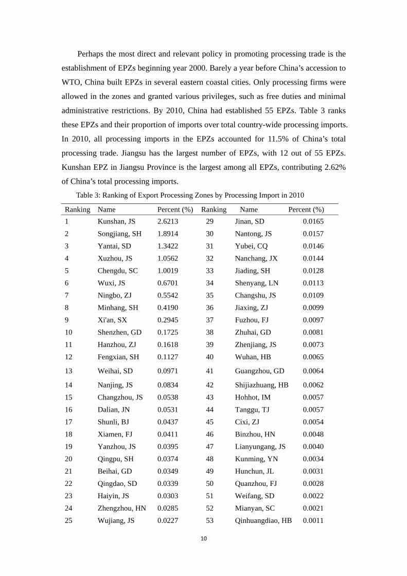
administrative restrictions. By 2010, China had established 55 EPZs. Table 3 ranks
these EPZs and their proportion of imports over total country-wide processing imports.
In 2010, all processing imports in the EPZs accounted for 11.5% of China’s total
processing trade. Jiangsu has the largest number of EPZs, with 12 out of 55 EPZs.
Kunshan EPZ in Jiangsu Province is the largest among all EPZs, contributing 2.62%
of China’s total processing imports.
Table 3: Ranking of Export Processing Zones by Processing Import in 2010
Ranking Name Percent (%) Ranking Name Percent (%) 1 Kunshan, JS 2.6213 29 Jinan, SD 0.0165
2 Songjiang, SH 1.8914 30 Nantong, JS 0.0157 3 Yantai, SD 1.3422 31 Yubei, CQ 0.0146 4 Xuzhou, JS 1.0562 32 Nanchang, JX 0.0144 5 Chengdu, SC 1.0019 33 Jiading, SH 0.0128 6 Wuxi, JS 0.6701 34 Shenyang, LN 0.0113 7 Ningbo, ZJ 0.5542 35 Changshu, JS 0.0109 8 Minhang, SH 0.4190 36 Jiaxing, ZJ 0.0099 9 Xi'an, SX 0.2945 37 Fuzhou, FJ 0.0097 10 Shenzhen, GD 0.1725 38 Zhuhai, GD 0.0081 11 Hanzhou, ZJ 0.1618 39 Zhenjiang, JS 0.0073 12 Fengxian, SH 0.1127 40 Wuhan, HB 0.0065
13 Weihai, SD 0.0971 41 Guangzhou, GD 0.0064
14 Nanjing, JS 0.0834 42 Shijiazhuang, HB 0.0062 15 Changzhou, JS 0.0538 43 Hohhot, IM 0.0057 16 Dalian, JN 0.0531 44 Tanggu, TJ 0.0057 17 Shunli, BJ 0.0437 45 Cixi, ZJ 0.0054 18 Xiamen, FJ 0.0411 46 Binzhou, HN 0.0048 19 Yanzhou, JS 0.0395 47 Lianyungang, JS 0.0040 20 Qingpu, SH 0.0374 48 Kunming, YN 0.0034 21 Beihai, GD 0.0349 49 Hunchun, JL 0.0031 22 Qingdao, SD 0.0339 50 Quanzhou, FJ 0.0028 23 Haiyin, JS 0.0303 51 Weifang, SD 0.0022 24 Zhengzhou, HN 0.0285 52 Mianyan, SC 0.0021 25 Wujiang, JS 0.0227 53 Qinhuangdiao, HB 0.0011
11
26 Wuhu, AH 0.0198 54 Ganzhou, JX 0.0004 27 Pudong, SH 0.0187 55 Urumqi, XJ 0.0002 28 Jiujiang, JX 0.0169
Source: China’s Customs Data (2010), Authors own compilation.
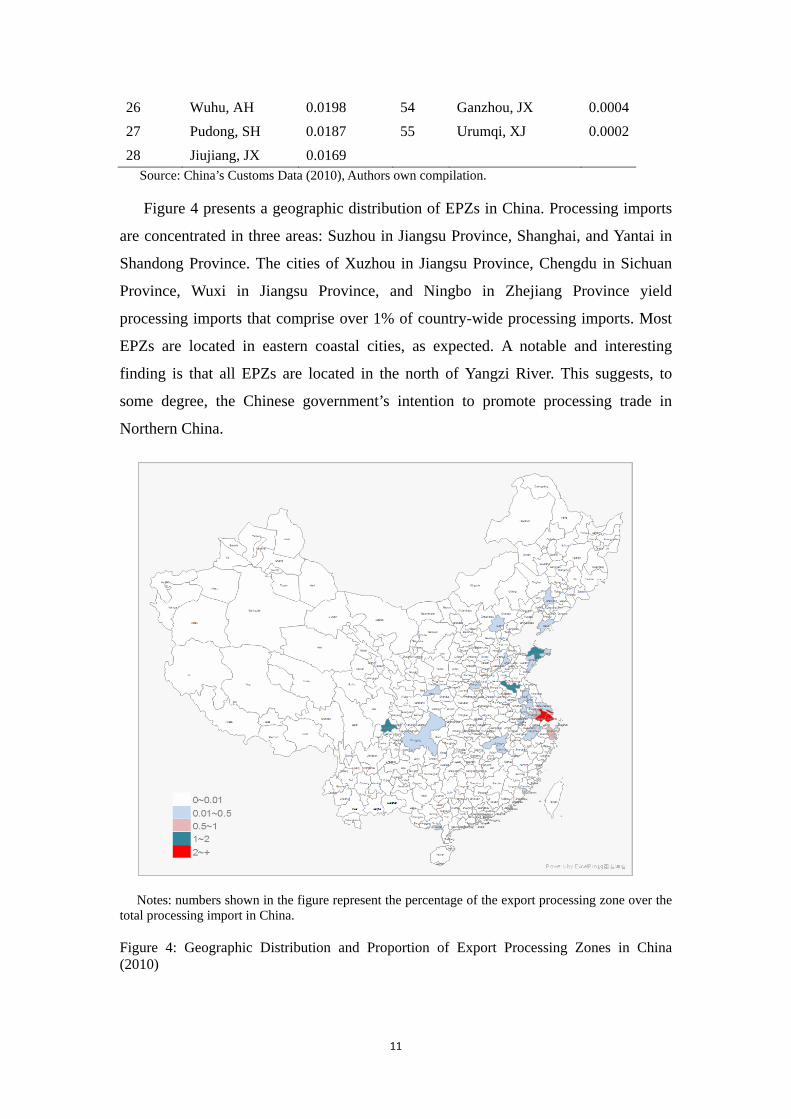
Figure 4 presents a geographic distribution of EPZs in China. Processing imports
are concentrated in three areas: Suzhou in Jiangsu Province, Shanghai, and Yantai in
Shandong Province. The cities of Xuzhou in Jiangsu Province, Chengdu in Sichuan
Province, Wuxi in Jiangsu Province, and Ningbo in Zhejiang Province yield
processing imports that comprise over 1% of country-wide processing imports. Most
EPZs are located in eastern coastal cities, as expected. A notable and interesting
finding is that all EPZs are located in the north of Yangzi River. This suggests, to
some degree, the Chinese government’s intention to promote processing trade in
Northern China.
Notes: numbers shown in the figure represent the percentage of the export processing zone over the total processing import in China.
Figure 4: Geographic Distribution and Proportion of Export Processing Zones in China (2010)

12
Aside from EPZs, other free-trade zones have contributed to the surge of
processing trade in China. Although China has only eight SEZs, processing imports in
these SEZs comprise over 3% of the country’s total processing trade, as illustrated in
Table 4.
Table 4: Ranking of Special Economic Zones by Processing Imports in 2010
Ranking Name Percent (%) Ranking Name Percent (%) 1 Shenzhen, GD 1.7464 5 Shantou, GD 0.0777 2 Zhuhai, GD 0.6235 6 Yunfu, GD 0.0538 3 Xiamen, FJ 0.5908 7 Other, HN 0.0152 4 Haikou, HN 0.1334 8 Sanya, HN 0.0029
Source: China’s Customs Data (2010), Authors own compilation.
Total processing imports from bonded areas is relatively small. There were five
bonded areas in China in 2010, namely, Tanggu, Pudong, Ningbo, Qingdao, and
Zhanjiagang. Only the bonded area of Tanggu, located in Tianjin Province, yielded a
relatively large share of processing imports (0.81%). Contributions from other bonded
areas are relatively economically insignificant. By way of comparison, hi-technology
industrial development areas (HTIDA) yield approximately 4% of China’s total
processing imports. As shown in Table 5, there are 49 HTIDA in China today, the
largest of which is Suzhou HTIDA in Jiangsu Province, which accounts for 1.38% of
China’s total processing imports, as exhibited in Table 5.
Table 5: Ranking of HTIDA by Processing Imports in 2010 Ranking Name Percent (%) Ranking Name Percent (%) 1 Suzhou, JS 1.3834 26 Minhang,SH 0.0043 2 Wuxi, JS 1.0092 27 Fengtai,BJ 0.0037 3 Guangzhou, GD 1.0063 28 Xianyang,SX 0.003
4 Huizhou, GD 0.228 29 Mianyang,SC 0.0029
5 Wuhan, HB 0.2104 30 Changping,BJ 0.0028
6 Xuhui, SH 0.1231 31 Jilin,JL 0.0024 7 Shenzhen, GD 0.085 32 Anshan,LN 0.0015
8 Baoding, HB 0.0838 33 Zhongshan,GD 0.0015
9 Xiamen, FJ 0.0819 34 Guilin,GX 0.001
10 Weihai, SD 0.0551 35 Jiulongpo,CQ 0.001
11 Haidion, BJ 0.0534 36 Xiangfan,HB 0.001 12 Nankai, TJ 0.0495 37 Nanjing,JS 0.0009

13
13 Shenyang, LN 0.0344 38 Chaoyang,BJ 0.0008
14 Chengdu, SC 0.0321 39 Weifang,SD 0.0006
15 Nanchang, JX 0.0311 40 Changsha,HN 0.0003
16 Xi'an, SX 0.0301 41 Zhengzhou,HN 0.0002
17 Dalian, LN 0.021 42 Lanzhou,GS 0.0001 18 Kunming,YN 0.0207 43 Zhuzhou,HN 0.0000 19 Hefei,AH 0.0147 44 Urumqi.XJ 0.0000
20 Changzhou,JS 0.0138 45 Shijiazhuang,HB 0.0000
21 Nanjing,JS 0.012 46 Jinan,SD 0.0000 22 Hangzhou,ZJ 0.0109 47 Nanning,GX 0.0000 23 Zibo,SD 0.0052 48 Guiyang,GZ 0.0000 24 Zhuhai,GD 0.0052 49 Taiyuan,SX 0.0000 25 Changchun,JL 0.0045
Source: China’s Customs Data (2010). Authors own compilation.
Economic and technological development areas (ETDA) are the leading zones for
processing imports. As shown in Table 6, Suzhou ETDA in Jiangsu Province accounts
for 4.83% of China’s total processing imports, which is significantly higher than that
accounted for by the largest EPZ, Kunshan EPZ in Jiangsu. Combined processing
imports from the 33 ETDAs (12.8%) are higher than that from the 55 EPZs (11.5%).
One possible reason is that EPZs were established much later than ETDAs were. This
implies that the absorption of processing imports takes time to materialize. Jiangsu
Province has outperformed other provinces in welcoming processing imports.
Table 6: Ranking of ETDA by Processing Imports in 2010
Ranking Name Percent (%)
Ranking Name Percent (%)
1 Suzhou,JS 4.8365 18 Shenyang,LN 0.034 2 Pudong,SH 2.1234 19 Taiyuan,SX 0.0277 3 Tanggu,TJ 1.4245 20 Hefei,AH 0.0277 4 Daxing,BJ 0.8821 21 Nanhui,SH 0.0258 5 Dalian,LN 0.8012 22 Lianyungang,JS 0.0252 6 Guangzhou,GD 0.7714 23 Wuhu,AH 0.0189 7 Yantai,SD 0.3768 24 Zhanjiang,GD 0.0117 8 Ningbo,ZJ 0.296 25 Changchun,JL 0.0047 9 Qingdao,SD 0.2247 26 Harbin,HLJ 0.0042 10 Other,HN 0.1621 27 Wenzhou,ZJ 0.0032 11 Fuzhou,FJ 0.1609 28 Nanan,CQ 0.001

14
12 Nantong,JS 0.1293 29 Chengdu,SC 0.0008 13 Hangzhou,ZJ 0.123 30 Xining,QH 0.0000 14 Wuhan,HB 0.0766 31 Yinchuan, NX 0.0000 15 Urumqi,XJ 0.0618 32 Shihezi, XJ 0.0000 16 Qinhuangdao, HB 0.0575 33 Changning, SH 0.0000 17 Minhang, SH 0.0469
Source: China’s Customs Data (2010). Authors own compilation.
In brief, the rapid growth of China’s processing trade is largely due to the
establishment of various free-trade zones, such as SEZs, ETDAs, HTIDAs, and EPZs,
in the last three decades. ETDAs and EPZs lead in terms of promoting processing
imports.
3. The Characteristics of Processing Trade
In this section, we discuss various characteristics of processing trade: the top 10
countries with which China imports processing intermediate inputs, top 10 industries
of processing imports, percent distribution of processing import by transport mode,
percent distribution of share of imports by ownership of firms, the scope of processing
firms, and the quality of processing imports. Processing imports, ordinary imports,
and total imports are compared. To realize comparison, we rely on transaction-level
trade data provided by China’s customs, which recorded around 3.3 million import
transactions in 2010. The data set includes information on customs district, location of
China’s importers, customs regime, countries of departure/origin, location of China’s
consumers, transport modes, HS 8-digit codes, quantity, and monthly values
(measured in US$). However, this data set does not include firm-level information.
Considering that firm-level analysis is critical to understanding China’s processing
trade from the micro-perspective, we resort to using transaction-level trade data
(2000–2006), which include firm-level information.
3.1 The Origin of Processing Imports
Our initial inquiry rests on the origin of processing imports. We compile customs
data for the year 2010 to determine the top 10 countries in terms of total imports,
processing imports, and ordinary imports. As shown in the last two columns of Table

15
7, China primarily imports from Japan, Korea, and Taiwan Province. China also
imports much from its entrepôt, Hong Kong and Macao. Although the United States
ranks only fifth in terms of total imports, it ranks next to Japan in terms of ordinary
imports. In terms of processing imports, Korea ranks first, followed by Hong Kong,
Japan, and Taiwan Province. This partly suggests that China imports core intermediate
inputs from Korea and Japan, and then exports final value-added products to the
United States and Europe.
Table 7: Ranking of Imports by Region by Customs Regime in 2010
Ranking Country Processing Imports (%)
Country Ordinary Imports (%)
Country Total
Imports (%) 1 Korea 14.97 Japan 11.77 Japan 12.80 2 China 14.43 United States 8.34 Korea 10.02 3 Japan 14.06 Germany 7.66 Taiwan 8.40 4 Taiwan 13.93 Australia 7.37 China 7.76 5 United States 6.17 Korea 5.95 United States 7.36 6 Malaysia 5.43 Brazil 4.58 Germany 5.40 7 Thailand 3.43 Taiwan 3.87 Australia 4.38 8 Germany 2.65 Saudi Arabia 3.41 Malaysia 3.66 9 Singapore 2.43 Angola 2.78 Brazil 2.77 10 Philippines 1.85 China 2.28 Thailand 2.41
Total 79.34 58.02 64.96 Source: China’s Customs Data (2010), Authors own compilation. Here proportions denote the
ratio of processing (ordinary, or both) imports by country over China’s total processing (ordinary, or both) imports in 2010. “China” here refers to imports from Hong Kong and Macao special administrative regions.
In terms of total import volume, the top 10 regions comprise two-thirds of China’s
total imports and 80% of China’s processing imports. The remaining 20% of
processing imports is produced by 200 trading partners in the rest of the world. The
next section discusses the kinds of products that China imports as intermediate inputs.
3.2 Top Products of Processing Imports
As shown in Table 8, the electrical machinery and transport equipment industry
yields the largest volume of processing imports, accounting for approximately 40% of
China’s total. Along with this industry, four other industries, namely, machinery and

16
mechanical appliance, optical and photographic instrument, mineral fuel and oil, and
plastic, account for approximately 70% of China’s total processing imports. These
five industries import a huge volume of intermediate inputs. However, it is still
worthwhile to investigate whether these industries adopt a large volume of domestic
inputs.
Table 8: Ranking of Imports by Industry in 2010
Ranking HS 2-Digit Proportion of Imports
HS 2-Digit Proportion of Imports
1 Electrical machinery & equipment 38.97 Electrical machinery & equipment 22.83 2 Machinery & Mechanical appliance 13.99 Mineral fuels, mineral oils 13.71 3 Optical, photographic instrument 10.25 Machinery & Mechanical appliance 12.51 4 Mineral fuels, mineral oils 5.98 Ores, slag, & ask 7.90 5 Plastics & articles thereof 5.44 Optical, photographic instrument 6.54 6 Copper & articles thereof 3.10 Plastics & articles thereof 4.63 7 Organic chemicals 2.35 Vehicles other than railway 3.60 8 Iron & steel 1.74 Organic chemicals 3.50 9 Rubber & articles thereof 1.59 Copper & articles thereof 3.35 10 Aircraft, spacecraft, and part 1.10 Oil seeds, industrial plants 1.97 Source: China’s Customs Data (2010), Authors own compilation. Here proportions denote the ratio of processing (or total) imports by HS 2-digit industry over China’s total processing (total) imports in 2010.
We calculate the ratio of imported intermediate inputs against total intermediate
inputs for several industries. Industrial intermediate inputs combine both imported
and domestic intermediate inputs. We utilize data on intermediate inputs maintained
by China’s customs bureau and China’s input-output data for year 2005 to calculate
the ratio of imported intermediate inputs. As shown in Figure 5, the five
aforementioned industries use a large amount of imported intermediate inputs (e.g.,
the ratio for machinery is 30%, whereas the ratio for non-metal minerals is 17%).

17
Source: cited from Yu (2011, ADB project)
Figure 5: Ratio of Imported Intermediate Inputs (2006)
3.3 Transportation Modes
There is ample evidence showing electrical machinery and transport equipment
commodities to be the most dominant among processing imports in China. How these
products reach China’s ports is another interesting question. Do these imports arrive
in China by sea, land, or air? We classify these imports by transport mode used in
2010. Six types of transport mode are identified in this paper: sea (or river if
applicable), railway, truck, air, post, and others. The last column of Table 9 shows that
62.52% of processing imports (in terms of value) reached China by sea in 2010,
suggesting sea shipment to be the prevailing mode of transportation. This observation
is consistent with the fact that most of China’s free-trade zones are located in its
eastern Pacific coast. The second most common transport mode is by air (19.63%)
and then by truck (15.72%).
Table 9: Proportion of Imports by Transport Mode in 2010 Transport Mode Processing Ordinary TotalBy Sea 41.47 79.81 62.52 By Railway 1.09 1.58 1.36 By Truck 27.42 6.12 15.72 By Air 29.56 11.47 19.63

18
By Post 0.01 0.04 0.03 Other 0.45 0.99 0.75
Source: China’s Customs Data (2010), Authors own compilation. Here proportions denote the ratio of processing (ordinary, or both) imports by transport mode over China’s total processing (ordinary, or both) imports in 2010.
The leading transport modes for all processing imports are the same as above. Sea
shipment accounts for 41%, whereas air shipment and truck shipment account for
29.56% and 27.42%, respectively. It is surprising to note that the percentage of air
shipment is higher than that of truck shipment because, intuitively, there should be
more commodities shipped by truck. However, the value of imports was used as
measurement, not the quantity of goods. The average per-unit price of commodities
sent by air shipment is usually higher than that of commodities sent by truck.
3.4 The Most Important Ports
We switch our interest to customs ports in China having the largest volume of total
imports, processing imports, and ordinary imports. The top 10 ports in terms of the
volume of processing imports in 2010 are Shanghai, Shenzhen, Nanjing, Qingdao,
Huangpu of Guangzhou, Guangzhou, Tianjin, Gongbei of Shanghai, Dalian, and
Beijing (Table 10). Except for Beijing, these ports are sea ports or river ports (e.g.,
Nanjing) located in the eastern Pacific coast. Shanghai port is the largest port not only
for processing imports but also for ordinary imports. Moreover, Shanghai port is the
largest port for total imports, followed by Shenzhen, a special economic zone located
in Guangdong Province.
Table 10: The Top 10 Ports with Largest Imports (2010) Ranking Ports Processing Ports Ordinary Ports Total Imports 1 Shanghai 22.57 Shanghai 15.99 Shanghai 18.97 2 Shenzhen 17.77 Qingdao 10.46 Shenzhen 12.64 3 Nanjing 15.23 Tianjin 8.57 Nanjing 11.38 4 Qingdao 9.19 Shenzhen 8.42 Qingdao 9.15 5 Huangpu 7.57 Nanjing 8.23 Huangpu 6.46 6 Guangzhou 3.40 Ningbo 6.10 Tianjin 6.14 7 Tianjin 3.19 Dalian 4.62 Ningbo 4.42 8 Gongbei 3.02 Huangpu 4.23 Dalian 3.80 9 Dalian 2.80 Hangzhou 4.05 Guangzhou 3.69

19
10 Beijing 2.78 Guangzhou 3.92 Beijing 3.38 Source: China’s Customs Data (2010). Authors own compilation
The top three ports with the largest share of processing imports are Shanghai,
Shenzhen, and Nanjing, comprising over 55% of China’s total processing imports.
This confirms that most processing imports are located in Shanghai, Guangdong, and
Jiangsu. In contrast, the top three ports with the most ordinary imports, namely,
Shanghai, Qingdao, and Tianjin, account for only 35% of China’s total ordinary
imports. This suggests that China’s processing imports are more concentrated than its
ordinary imports.
3.5 The Top Strongly-Demanded Location
We examine the destination of processing imports in China. Most processing
goods are imported through Shanghai, Shenzhen, and Nanjing, so a natural conjecture
is that processing importers are concentrated in these areas. Processing firms would
choose their closest ports to reduce transport costs. To verify this conjecture, we
determine the top 10 strongly-demanded cities/districts using China’s
transaction-level trade data in 2010.
Table 11: The Top 10 Strongly-Demanded Cities (2010) Ranking City Processing City Ordinary City Total Imports1 Shenzhen, GD 7.40 Chaoyang, BJ 10.05 Chaoyang, BJ 6.41 2 Pudong, SH 6.11 Xicheng, BJ 5.71 Shenzhen, GD 3.58 3 Suzhou, JS 4.56 Haidian,BJ 3.06 Pudong, SH 3.27 4 Dongguan, GD 3.64 Chaoyang, BJ 2.87 Mentougou, BJ 3.22 5 Shenzhen, GD 2.38 Pudong, SH 1.76 Suzhou, JS 2.38 6 Chaoyang, BJ 1.98 Shenzhen, GD 1.47 Dongguan, GD 1.89 7 Songjiang, SH 1.74 Guangzhou, GD 1.13 Haidian, BJ 1.71 8 Dongguan, GD 1.74 Pudong, SH 1.06 Chanyang, BJ 1.58 9 Kunshan, JS 1.24 Shenzhen, GD 0.95 Pudong, BJ 1.33 10 Dongguan, GD 1.09 Pudong, SH 0.93 Shenzhen, GD 1.08
Source: China’s Customs Data (2010). Authors own compilation. Sometimes a city is displaced more than once since it could contain firms in different zones such as EPZ, ETDA, and HTIDA.
Shenzhen, Pudong, and Suzhou prove to be the top three districts or areas with the
most processing imports. However, they account for only 18% of total processing
imports. The leading destinations of processing imports are different from the leading

20
destinations of ordinary imports (i.e., Chaoyang, Xicheng, and Haidian, which are all
in Beijing). One possible explanation is that ordinary imports include more final
consumption goods, whereas processing imports include mostly intermediate goods.
Combining processing imports and ordinary imports, Chaoyang of Beijing replaces
Shenzhen and Pudong as the top import destination in 2010, receiving 6.41% of total
imports in China.
3.6 Quality of Processing Imports
Another interesting issue is the quality of processing imports. China imports raw
materials from many trading partners, so which countries ship products with the
highest quality? Which goods have higher quality? Answering these questions
requires coming up with an appropriate measure of the quality of goods, which is a
challenging task (Khandelwal, 2010). A common gauge is the per-unit value of
products (Hallak, 2006), which is obtained by dividing a good’s value by its quantity.
Figure 6 shows the top 10 countries that ship goods with the highest quality to
China. Interestingly, nine out of these ten countries (regimes) are located in Europe.
The top five countries are as follows: Norway, France, Finland, Germany, and
Netherlands. The United States ranks sixth. Meanwhile, the top five countries
(regimes) with the highest quality of ordinary imports are Cayman Island, Finland,
Germany, Panama, and Austria. Cayman Island is capable of exporting high-quality
products due to its “tax-haven” privileges. Certain countries can export their products
to Cayman Island, which serves as an entrepôt, for eventual shipment to China.

21
Notes: The color areas denotes the top 10 countries (regimes) that with highest product quality for processing goods shipped to China in 2010: Norway, France, Finland, Germany, Netherlands, the United States, Austria, Switzerland, Italy, and Denmark.
Figure 6: The Top 10 Countries with Highest Quality for Processing Goods Shipped to China
Table 12 lists industries that lead in terms of importing high-quality raw materials
for processing. Imports from the aircraft and spacecraft industry have the largest
per-unit value at approximately $2.39 million, followed by ships and boats, and
machinery and mechanical appliances. The table likewise shows very high differences
in the per-unit value of products imported by the top three importing industries.
Table 12: Top 10 industries with Highest Quality for Processing Imports (2010)
Code Descriptions of HS 2-Digit Codes Unit Value 88 Aircraft, spacecraft, and parts thereof 2,398,441 89 Ships, boats and floating structures 482,843 84 Nuclear reactors, boilers, machinery and mechanical appliances 42,994 90 Optical, photographic, medical or surgical instruments 17,576 87 Vehicles other than railway or tramway rolling-stock 13,083 86 Railway or tramway locomotives, rolling-stock and parts 3,493 85 Electrical machinery & equipment and parts thereof 2,890 30 Pharmaceutical Products 1,064 92 Musical Instruments, parts and accessories 878 81 Other base metals, cermet, articles thereof 727
Sources: China’s Customs Data (2010). Authors’ own compilation.
3.7 Ownership of Processing Importing Firms

22
Thus far, we have gained some understanding of China’s processing imports from
the industrial perspective, specifically the origin countries, main products, transport
mode, entry ports, consumption destinations, and even quality of commodities. Now,
we take a step forward to understand the micro-mechanism. In particular, we explore
what types of firms frequently engage in processing trade. In terms of ownership,
what types of firms account for the largest proportion of China’s processing imports?
We use China’s customs transaction-level data in 2010 to answer this question.
Table 13: Proportion of Imports by Ownership of Firms in 2010 Firm Types Processing Ordinary Total State-owned enterprise 12.24 41.23 28.16 Sino-foreign contractual joint venture 0.66 0.44 0.54 Sino-foreign equity joint venture 16.53 14.14 15.22 Foreign-invested enterprise 58.76 20.70 37.86 Collective enterprise 1.42 3.45 2.54 Private enterprise 10.17 20.00 15.57 Other, including foreign company's office in China 0.01 0.01 0.01 Source: China’s Customs Data (2010), Authors own compilation. Here proportions denote the ratio of
processing (ordinary, or both) imports by ownership of firms over China’s total processing (ordinary, or both) imports in 2010.
As shown in Table 13, over half of processing imports are attributable to foreign-invested
enterprises. Another 17% of processing imports are attributable to Sino-foreign joint ventures
(either contractual or equity joint ventures). State-owned and private enterprises only account for a
relatively small proportion (12.2% and 10.2%, respectively). Meanwhile, state-owned enterprises
are the most important type of firms involved in ordinary imports (second column of Table 12).
Combining both processing and ordinary imports (last column of Table 10), foreign-invested
enterprises are the most important type of importers (37.86%), followed by state-owned
enterprises (28.16%).
3.8 Scopes for Processing Importing Firms
How many varieties do processing firms import? Compared to ordinary importing firms, do
processing firms import more varieties? Answering these questions requires a data set containing
firm-level information. China’s 2010 customs data set (the most recently released version) does

23
not include such information. As a compromise, we have to rely on previous data sets. We
therefore adopt China’s transaction-level trade data in 2000–2006, which include firm-level
information, such as firm name, address, zip code, and telephone numbers.
Sources: The figure is cited from Yu (2011). Dotted lines represent firms’ processing imports
(exports) whereas real lines denote firms’ non-processing (i.e., ordinary) imports (exports).
Figure 7: Four Types of Firms in China
Before investigating the importation scope of processing firms, we also need to provide a
formal definition of such firms. Yu (2011) classified firms in China into four types as shown in
Figure 7: (1) non-importing firms that do not use any foreign intermediate inputs; (2)
non-processing importing firms that could use some foreign intermediate inputs but do not sell
their final products abroad; (3) hybrid (or regular) processing firms that could engage in both
processing and ordinary imports; and (4) pure processing firms that only engage in processing
imports and exports, and do not sell their products in the domestic market. In the present paper, we
define both hybrid and pure processing firms as processing importers. In other words, a firm
engaging in some processing imports is labeled as a processing firm.
Table 14A: The Scope of Importing Firms by Year (2000-2006)
Scope 2000 2001 2002 2003 2004 2005 2006 1 19.04 18.9 19.76 20.32 21.65 22.66 23.6

24
2 10.27 10.14 10.55 10.77 11.43 11.97 12.19 3 6.67 7.15 7.23 7.34 7.66 7.93 8.1 4 5.26 5.39 5.42 5.76 5.64 5.78 5.96 5 4.38 4.41 4.5 4.62 4.63 4.65 4.62 6 3.61 3.87 3.9 3.79 3.8 3.69 3.76 7 3.29 3.26 3.34 3.34 3.2 3.17 3.2 8 2.98 2.89 2.89 2.81 2.79 2.7 2.73 9 2.44 2.66 2.54 2.53 2.49 2.38 2.34 10 2.33 2.35 2.36 2.26 2.12 2.13 2.11 11-50 31.21 30.68 28.23 28.24 26.71 25.74 24.51 51-100 5.05 4.23 4.9 4.97 4.78 4.43 4.34 101-1000 3.24 3.1 2.94 2.99 2.86 2.58 2.34 >1000 0.23 0.97 1.34 0.26 0.24 0.19 0.2 maximum 3497 3404 3321 3211 3070 3023 2839
Sources: China’s Customs Data (2000-2006). Authors’ own calculation.
Table 14A reports the scope of processing trade by year. In 2000–2006, around 20% of firms
imported only a single variety, and around 10% imported two varieties. In 2000, around 45%
imported less than 5 varieties, whereas around 50% imported less than 10 varieties. Another 31%
imported more than 10 but less than 50 varieties. The other 3.24% imported more than 50 but less
than 1,000 varieties. Only 0.23% of the firms imported more than 1,000 varieties, with 3,497 as
the highest number of varieties imported.
Table 14A also shows the dynamic pattern for each cohort. In the same period, the proportion
of firms importing less than 5 varieties increased from 45% to 54%. Similarly, the proportion of
firms importing less than 10 varieties increased from 60% to 68%. In contrast, the proportion of
firms importing more than 10 varieties but less than 50 varieties declined from 31.2% to 24.5%.
The highest number of varieties imported also declined to 2,839 in 2006.
Table 14B: The Scope of Processing Importing Firms by Year (2000-2006)
Scope 2000 2001 2002 2003 2004 2005 2006 1 20.6 20.34 21.6 22.37 23.41 24.4 25.42 2 10.69 10.56 11.09 11.45 11.71 11.97 12.32 3 6.82 7.21 7.39 7.66 7.7 7.98 8.07 4 5.42 5.7 5.55 5.78 5.77 5.86 6.07 5 4.53 4.57 4.67 4.83 4.72 4.69 4.69 6 3.69 4.06 3.9 3.95 3.87 3.88 3.81

25
7 3.38 3.32 3.47 3.35 3.46 3.25 3.33 8 2.9 2.95 2.86 2.99 2.98 2.79 2.75 9 2.63 2.72 2.68 2.5 2.54 2.5 2.45 10 2.32 2.44 2.44 2.34 2.29 2.21 2.16 11-50 31.04 30.62 29.37 27.93 26.73 25.96 24.51 51-100 3.96 3.73 3.45 3.36 3.37 3.09 3.1 101-1000 1.83 1.58 1.34 1.3 1.3 1.27 1.18 >1000 0.19 0.2 0.19 0.19 0.15 0.15 0.14 maximum 3489 3397 3319 3199 3070 3023 2836
Sources: China’s Customs Data (2000-2006). Authors’ own calculation.
Processing and non-processing firms share a similar importation scope pattern. However, more
processing firms import a single variety than non-processing firms. In 2006, the proportion of
single-variety processing importers (25.4%) was higher than that of single-variety non-processing
importers (23.6%). In the same year, the proportion of processing firms (4.42%) importing more
than 50 varieties was lower that of non-processing firms (6.88%), as shown in Table 13A.
Sources: China’s Customs Data (2000-2006). Authors’ own compilation.
Figure 8: The Maximum of Scope for Importing Firms and Processing Importing Firms
Figure 8 shows that the number of varieties that firms import declines over time. Such a
pattern is true for both processing and ordinary importers. For most years in the sample,
processing firms have imported fewer varieties than ordinary firms. Thus, the highest number of
varieties for all importers is higher than that for processing importers only.
26
Thus far, we have understood that processing firms mostly come from Korea, Hong Kong, and
Japan. The industry with the largest processing imports is electrical machinery and transport
equipment. Most of the processing imports are shipped to China by sea and air. The top three
busiest customs ports for processing imports are Shanghai, Shenzhen, and Nanjing, whereas the
top three districts/areas that have the most processing imports are Shenzhen, Pudong, and Suzhou.
The industry with the highest per-unit value of commodities is the aircraft and spacecraft industry.
The top five countries with the highest quality of goods shipped to China for processing are all
located in Europe: Norway, France, Finland, Germany, and Netherlands. In terms of types of
importer ownership, foreign-invested enterprises are the top importers of processing goods.
Around 20% of processing firms only import a single variety, and around 50% import less than 10
varieties. Furthermore, the number of imported varieties declines over time. However, an
important question is still unanswered: do processing firms have higher (or lower) productivity
than non-processing firms? We now seek to answer this question.
4. Matching Transaction-Level Trade Data and Firm-Level Production Data
To explore processing firms’ productivities, we need data on processing firm’s output
level and labor. If productivity is measured as total factor productivity, we also need
data on capital and intermediate inputs. Transaction-level trade data offer rich
information but do not contain information on production factors, such as output and
input factors. Hence, we have to appeal to firm-level production data and use a
merged data set. Below, we begin by describing two data sets, and we present a
detailed technique for their merging. Thereafter, we discuss the performance of the
matched data set. Indeed, the two data sets are widely accepted in the study of China’s
foreign trade and firm heterogeneity. Yet, as far as we know, very few papers offer a
detailed and reliable means to discuss the matching of these two data sets. Thus, our
paper aims to fill a research gap on the heterogeneity of Chinese firms.
4.1 Transaction-level Trade Data Set
Extremely disaggregated transaction-level monthly trade data for 2000–2006 are
obtained from China’s General Administration of Customs. Each transaction is
described at the HS 8-digit level. The number of monthly observations increased from

27
around 78,000 in January 2000 to more than 230,000 in December 2006. As shown in
Column (1) of Table 15, the annual number of observations is over 10 million in 2000
and 16 million in 2006, ending with a huge number of observations (118,333,831 in
total) for seven years. Column (2) of Table 14 shows that 286,819 firms engaged in
international trade during this period.
For each transaction, the data set compiles three types of information: (1) five
variables on basic trade information, including value (measured in US current dollar),
trade status (export or import), quantity, trade unit, and value per unit (value divided
by quantity); (2) six variables on trade mode and pattern, including country of
destination for exports, country of origin for imports, routing (whether the product is
shipped through an intermediate country/regime), customs regime (processing trade or
ordinary trade), trade mode (by sea, truck, air, or post), and customs port (where the
product departs or arrives); and (3) seven variables on firm information associated
with each transaction, including firm name, identification number set by customs,
Chinese city where the firm is located, telephone number, zip code, name of the
manager/CEO, and ownership type of firm (foreign affiliate, private, or state-owned).
4.2 Firm-level Production Data Set
The sample used in this paper comes from a rich firm-level panel data set covering
around 230,000 manufacturing firms per year for the years 2000–2006. The number
of firms doubled from 162,885 in 2000 to 301,961 in 2006. The data, including full
information on three accounting sheets (i.e., balance, loss and benefit, and cash flow
sheets) are collected through an annual survey of manufacturing enterprises and
maintained by China’s National Bureau of Statistics. On average, the annual entire
value of industrial production covered by such a data set accounts for around 95% of
China’s total annual industrial production. Aggregated data on the industrial sector in
China’s Statistical Yearbook from the Natural Bureau of Statistics (NBS) are compiled
from this data set. The data set includes over 100 financial variables listed in the main
accounting sheets of all covered firms. Briefly, two types of manufacturing firms are
covered: all SOEs and all non-SOEs with annual sales more than five million RMB.
The number of firms increased from over 160,000 in 2000 to 301,000 in 2006. As

28
shown in Column (3) of Table 15, the number of firms that were included in the data
set at any time in 2000–2006 is 615,951 in total.
However, the raw production data set still has quite some noise given that many
unqualified firms are included, largely due to misreporting by some firms. For
example, information on some family-based firms, which usually have no formal
accounting system in place, is based on a unit of one RMB, whereas the official
requirement is a unit of 1,000 RMB. Following Cai-Liu (2009) and Feenstra-Li-Yu
(2011), we delete observations according to generally accepted accounting principles
if any of the following are true: (1) liquid assets are higher than total assets; (2) total
fixed assets are larger than total assets; (3) the net value of fixed assets is larger than
total assets; (4) the firm’s identification number is missing; or (5) an invalid
established time exists (e.g., the opening month is later than December or earlier than
January). Accordingly, the total number of firms covered in the data set is reduced to
438,165, and around one-thirds of firms are dropped from the sample after such a
filtering process. As shown in Column (4) of Table 15, the filter ratio is even higher in
the initial years: around one-half of firms in 2000 are dropped.
4.3 Matching Method
Although the two available data sets have rich information on production and
trade, matching them is challenging. Both data sets contain firm identification
numbers. However, the coding systems in these data sets are completely different. For
example, the length of firm IDs in the transaction-level data set is 10 digits, whereas
that in the firm-level data set is only 9 digits. China’s customs administration has a
coding system that is completely different from that adopted by the National Bureau
of Statistics.
We go through two stages to match transaction-level trade data with firm-level
production data. In the first stage, we match the two data sets by firm name and year.
If a firm has an exact Chinese name in both data sets in a particular year, they should
be the same firm. The year variable is necessary as an auxiliary identification variable
because some firms could have different names across years, and newcomers could
possibly take their original names. Using the raw production data set, we come up

29
with 83,679 matching firms; this number is further reduced to 69,623 with the more
accurate filtered production data set.
In the second stage, we use another matching technique as supplement. Here, we
rely on two other common variables to identify firms, namely, zip code and the last
seven digits of a firm’s phone number. The rationale is that firms should have
different and unique phone numbers within a postal district. Although this method
seems straightforward, subtle technical and practical difficulties still exist. For
example, the production-level trade data set includes both area phone codes and a
hyphen in phone numbers, whereas the firm-level production data set does not.
Therefore, we use the last seven digits of the phone number to serve as proxy for firm
identification for two reasons. First, in 2000–2006, some large Chinese cities added
one more digit at the start of their seven-digit phone numbers. Therefore, sticking to
the last seven digits of the number will not confuse firm identification. Second, in the
original data set, phone number is defined as a string of characters with the phone zip
code. However, it is inappropriate to de-string such characters to numerals because a
hyphen is used to connect the zip code and phone number. Using the last seven-digit
substring neatly solves this problem.
A firm could miss its name information in either trade or production data set.
Similarly, a firm could lose its phone and/or zip code information. To assure that our
matched data set can cover as many common firms as possible, we then include
observations in the matched data set if a firm occurs in either the name-adopted
matched data set or the phone-and-post-adopted matched data set. The number of
matched firms increases to 90,558 when the raw production data set is used, as shown
in Column (7) of Table 15. Our matching performance is comparable to (or even
better than) that of other similar studies. For example, Ge et al. (2011) used the same
data sets and similar matching techniques, but ended up with 86,336 matching firms.
Meanwhile, if we match the more rigorously filtered production data set with the
firm-level data set, we end up with 76,823 firms in total, as shown in the last column
of Table 15.

30
Table 15: Matched Statistics--Number of Firms Year Trade Data Production Data Matched Data
Number Transactions Firms Raw Filtered w/ Raw w/ Filtered w/ Raw w/ Filtered
Firms Firms Firms Firms Firms Firms
(1) (2) (3) (4) (5) (6) (7) (8)
2000 10,586,696 80,232 162,883 83,628 18,580 12,842 21,665 15,748
2001 12,667,685 87,404 169,031 100,100 21,583 15,645 25,282 19,091
2002 14,032,675 95,579 181,557 110,530 24,696 18,140 29,144 22,291
2003 18,069,404 113,147 196,222 129,508 28,898 21,837 34,386 26.930
2004 21,402,355 134,895 277,004 199,927 44,338 35,007 50,798 40,711
2005 24,889,639 136,604 271,835 198,302 44,387 34,958 50,426 40,387
2006 16,685,377 197,806 301,960 224,854 53,748 42,833 59,133 47,591
All Year 118,333,831 286,819 615,951 438,165 83,679 69,623 90,558 76,823
Notes: Column (1) reports number of observations of HS eight-digit monthly transaction-level trade data from
China's General Administration of Customs by year. Column (2) reports number of firms covered in the
transaction-level trade data by year. Column (3) reports number of firms covered in the firm-level production
dataset compiled by China's National Bureau of Statistics without any filter and cleaning. By contrast, Column (4)
presents number of firms covered in the firm-level production dataset with careful filter according to the
requirement of GAAP. Accordingly, Column (5) reports number of matched firms using exactly identical
company's names in both trade dataset and raw production dataset. By contrast, Column (6) reports number of
matched firms using exactly identical company's names in both trade dataset and filtered production dataset.
Finally, Column (7) reports number of matched firms using exactly identical company's names and exactly
identical zip code and phone numbers in both trade dataset and raw production dataset. By contrast, Column (8)
reports number of matched firms using exactly identical company's names and exactly identical zip code and
phone numbers in both trade dataset and filtered production data set.
How is the performance of our matched data set? Table 16 compares several key
firm-level variables between the matched data set and the full-sample production data
set. The matched sample clearly has higher means of sales, exports, number of
employees, log of capital-labor ratio, and even log of labor productivity compared
with the full sample, suggesting that the merged sample is skewed toward large firms.
By construction, the full-sample firm-level production data set contains only large
firms (i.e., with annual sales larger than $770,000), and our matched data set contains
around 70% of total exports. Thus, our matched data set is sufficiently representative

31
of large Chinese exporting firms.
Table 16: Comparison of the Merged Dataset and the Full-sample Production Dataset Variables Matched Data set Full-sample Production Data set Mean Min. Max. Mean Min. Max.
Sales 156,348 5000 1.57e+08 85,065 5000 1.57e+08
Exports 51,751 0 1.52e+08 16,544 0 1.52e+08
Number of Employees 479 10 157,213 274 10 165,878
Log of Capital-Labor Ratio 3.62 -5.71 9.87 3.53 -6.22 11.14
Log of Labor Productivity 3.86 -7.75 10.78 3.84 -8.96 10.79
Sources: Cited from Qiu and Yu (2012).
5. Productivity for Processing Firms
With a matched trade and firm-level production data set, we are now ready to explore the
productivity of processing firms. Labor productivity is a simple and straightforward measure
of productivity. However, labor productivity cannot measure the contribution of input factors
other than labor. As such, total factor productivity (TFP) is a better measure because it
captures contributions from all input factors.
The TFP literature usually suggests using the Cobb–Douglas production function to
introduce technology improvement:
,l
km
ititititit LKMYβββπ= (1)
Where Yit, Mit, Kit, Lit is firm i's output, materials, capital, and labor at year t , respectively.
To measure firm's TFP, it, one needs to estimate (1) by taking a log function first:
ln Yit 0 m ln Mit k ln Kit l ln Lit it, (2)
Traditionally, TFP is measured by the estimated Solow residual between the true data on
output and its fitted value, ln Yit . That is:
TFPit ln Yit − ln Yit. (3)

32
However, this approach suffers from two problems: simultaneity bias and selection bias. As
first suggested by Marschak and Andrews (1944), at least some parts of TFP changes could be
observed by firms early enough for them to change their input decisions and maximize profit.
Thus, TFP could have reverse endogeneity in its input factors. The lack of such a consideration
would make the maximized choice of firms biased. In addition, the dynamic behavior of firms also
introduces selection bias. With international competition, firms with low productivity would die
and exit the market, whereas those with high productivity would remain (Melitz, 2003). In a panel
data set, the firms observed are those that have already survived. Meanwhile, firms with low
productivity, which collapsed and exited the market, are excluded from the data set. This means
that the firms included in the regression are not randomly selected, resulting in estimation bias.
Econometricians have strived to address the empirical challenge of measuring TFP but have
been unsuccessful until the pioneering work of Olley and Pakes (1996). In the beginning,
researchers used two-way (firm-specific and year-specific) fixed effects estimations to mitigate
simultaneity bias. Although the fixed-effect approach controls for several unobserved productivity
shocks, it does not offer much help in dealing with reverse endogeneity and thus remains
unsatisfactory. Similarly, to mitigate selection bias, one might estimate a balanced panel by
dropping observations that have disappeared during the investigation. The problem is that a
substantial part of the information contained in the data set is wasted, and the dynamic behavior of
firms is completely unknown.
Fortunately, the Olley–Pakes methodology contributes significantly in addressing the
challenge of TFP measurement. Assuming that the expectation of the future realization of the
unobserved productivity shock, itυ , relies on its contemporaneous value, a firm i ’s investment
is modeled as an increasing function of both unobserved productivity and log capital,
itit Kk ln≡ . Following previous studies, such as van Biesebroeck (2005) and Amiti and Konings
(2007), we revise the Olley–Pakes approach by adding the export decisions of firms as an extra
argument in the investment function because most export decisions are determined in the previous
period (Tybout, 2003):

33
),,,,(ln~ititititit IFEFKII υ= (4)
where itEF ( itIF ) is a dummy variable measuring whether firm i exports (imports) at year t .
Therefore, the inverse function of investment is ),,,(ln~ 1ititititit IFEFIKI −=υ .5 Unobserved
productivity also depends on log capital and firm i ’s export decisions. Accordingly, Estimation
Specification (1) can now be written as
,),,,(lnlnlnln 0 ititititititlitmit IFEFIKgLMY εβββ ++++= (6)
Wwhere ),,(ln ititit EFIKg is defined as ),,(ln~ln 1ititititk EFIKIK −+β . Following Olley
and Pakes (1996) and Amiti and Konings (2007), fourth order polynomials are used in log-capital,
log-investment, export dummy, and import dummy to approximate ).(⋅g 6 In addition, our firm
data set covers the period 2000–2006, so we include a WTO dummy (i.e., one for a year after
2001 and zero for before) to characterize the function )(⋅g as follows:
.)1(),,,,(4
0
4
0
qit
hithq
qhititttitititit IkIFEFWTOWTOIFEFIkg δ∑∑
==
+++= (7)
After finding the estimated coefficients mβ and lβ , we calculate the residual itR which is
defined as itlitmitit LMYR lnˆlnˆln ββ −−≡ .
The next step is to obtain an unbiased estimated coefficient of kβ . Amiti and Konings (2007)
suggested estimating the probability of a survival indicator on a high-order polynomial in
log-capital and log-investment to correct selection bias as mentioned above. We can then
5 Olley and Pakes (1996) showed that the investment demand function is monotonically increasing
in the productivity shock ikυ , by making some mild assumptions on the production technology of
firms.
6 Using higher-order polynomials to approximate )(⋅g does not change the estimation results.

34
accurately estimate the following specification:
,)ˆ,ln(~ln 1,1,1,1
ittitiktiitkit rpKgIKR εββ +−+= −−−−
(8)
where irp is the fitted value of the probability of firm i ’s exit in the next year. The specific
“true” functional form of the inverse function )(~ 1 ⋅−I is unknown, making it appropriate to use
fourth order polynomials in 1, −tig and 1,ln −tiK as approximation. In addition, Equation (8) requires
the estimated coefficients of the log-capital in the first and second terms to be identical. Therefore,
non-linear least squares seem to be the most desirable econometric technique (Pavcnik, 2002;
Arnold, 2005). Finally, the Olley–Pakes type of TFP for each firm i in industry j is obtained
once the estimated coefficient kβ is obtained:
.lnˆlnˆlnˆln itlitkitmitOP
ijt LKMYTFP βββ −−−= (9)
As discussed above, the revised Olley–Pakes approach assumes that capital responds to
unobserved productivity shock with a Markov process, whereas other input factors do so without
any dynamic effects. However, labor may be correlated with unobserved productivity shocks as
well (Ackerberg et al., 2006). This consideration may fit with China’s case very closely, given that
China is a country with abundant labor. When facing unobserved productivity shocks, firms might
prefer adjusting their labor rather than their capital to re-optimize their production behavior. We
then use the Blundell–Bond (1998) system GMM approach to capture the dynamic effects of other
input factors. Assuming that the unobserved productivity shock depends on firm i ’s previous
period realizations, the system GMM approach models TFP to be affected by all types of firm i ’s
inputs in both current and past realizations.7 In particular, this model has a dynamic representation
7 Note that the first-difference GMM introduced by Arellano and Bond (1991) also allows a firm’s output to depend on its past realization. However, such an approach would lose instruments for the factor inputs because the lag of output and factor inputs are correlated with past error shocks and the autoregressive error term. In contrast, by assuming that the first difference of instrumented variables is uncorrelated with the fixed effects, the system GMM approach can introduce more instruments and thereby dramatically improve efficiency.

35
as follows:
ln yit 1 ln Lit 2 ln Li,t−1 3 ln Kit 4 ln Ki,t−1 5 ln Mit
6 ln Mi,t−1 7 ln yi,t−1 i t it, (10)
wherei is firm i ’s fixed effect and t is the year-specific fixed effect. The idiosyncratic term
it is serially uncorrelated if no measurement error exists.8 We can obtain consistent estimates
of the coefficients in (12) using a system GMM approach. The idea is that labor and material
inputs are not taken as exogenously given. Instead, they are allowed to change over time as capital
grows. Although the system GMM approach still faces a technical challenge to control for
selection bias when a firm exits, using this approach to estimate a firm’s TFP as a robustness
check is still worthwhile.
Table 17 summarizes the estimates of the Olley–Pakes input elasticity of Chinese firms at the
HS two-digit level. We first cluster the 97 HS two-digit industries into 15 categories and calculate
their estimated probability and input elasticity. The estimated survival probability of a firm in the
next year varies from 0.977 to 0.996, with a mean of 0.994, suggesting that firm exits are less
severe in the sample and in the given period.9
Table 17 presents differences in the estimated coefficients for labor, materials, and capital using
both the Olley–Pakes methodology and the system GMM approach. The last row of Table 17
suggests that, on average, the Olley–Pakes approach yields a higher elasticity of capital
(kOP . 117, k
GMM . 001), whereas the system GMM approach yields a higher elasticity of labor
(lOP . 052, l
GMM . 240). Summarizing all the estimated elasticity, the implied scale elasticity is
8 As discussed by Blundell and Bond (1998), even if there is a transient measurement error in some of
the series (i.e.,it ~MA1 ), the system GMM approach can still reach consistent estimates of the coefficients in (6). 9 Note that here, firm exit means a firm either stops trading and exits the market, or simply has an annual sales figure lower than the “large scale” amount (five million RMB in sales per year) and dropped from the data set. Owing to data set restrictions, we cannot distinguish the difference between the two.

36
0.989 using the Olley–Pakes approach, 10 which is close to the constant returns-to-scale
elasticity.11 Turning to the comparison between the OLS and Olley–Pakes approaches, the
estimates suggest that the usual OLS approach has a downward bias
(TFPOLS . 958; TFPOP 1. 188) largely because of the lack of control for simultaneity bias and
selection bias.
Finally, for a cross-country comparison of the Olley–Pakes estimates, the estimation results
suggest that intermediate inputs are more important for Chinese firms than for American firms
(Keller and Yeaple, 2009) or for Indonesian firms (Amiti and Konings, 2007). However, the
elasticity of capital input is less important for Chinese firms than for American or Indonesian
firms. This implies that processing trade does play a significant role in China’s productivity
growth.
Table 17: Estimates of Olley-Pakes Input Elasticity of Chinese Firms HS 2-digit Labor Materials Capital
OP GMM OP GMM OP GMM
Animal Products (01-05) .056** .053 .888** .970** .048** -.022
(3.32) (.87) (55.36) (17.71) (1.80) (-.43)
Vegetable Products (06-15) .007 .031** .891** .571** .052** .019
(.49) (8.55) (68.05) (9.82) (5.49) (.46)
Foodstuffs (16-24) .036** -.020 .874** .595** .044 .027
(2.23) (-.25) (68.48) (10.73) (1.07) (.46)
Mineral Products (25-27) .035* .241** .872** .671** .099** .089
(1.70) (3.78) (51.00) (15.51) (2.69) (1.57)
Chemicals & Allied .014** .127** .831** .488** .103** .071
Industries (28-38) (1.98) (1.95) (121.70) (10.99) (7.79) (1.48)
Plastics / Rubbers (39-40) .064** .321** .796** .298** .103** -.003
10 This is calculated as . 052 . 820 . 117 . 989 using the Olley–Pakes approach.
11 Note that here, we use the industrial deflator as proxy of a firm’s price. Indeed, it is even possible that Chinese firms exhibit the increasing returns-to-scale property in the new century when the actual prices of firms are used to calculate “physical” productivity. This is a possible future research topic provided that relevant data are available.

37
(8.49) (6.98) (107.17) (4.54) (5.59) (-.08)
Raw Hides, Skins, Leather .102** .125* .810** .738** .090** .043
& Furs (41-43) (7.76) (1.85) (65.53) (11.55) (3.36) (.66)
Wood Products .039** .041 .855** .266** .012 .118**
(44-49) (4.29) (.46) (97.11) (6.83) (.47) (2.99)
Textiles (50-63) .085** .157** .810** .653** .066** .043*
(19.50) (4.81) (192.59) (22.96) (10.38) (1.95)
Footwear / Headgear (64-67) .072** .138 .864** .703** .033** .108**
(5.93) (1.62) (73.17) (10.77) (5.43) (2.38)
Stone / Glass (68-71) .104** .233** .785** .448** .103** .063
(9.14) (3.56) (67.02) (11.58) (8.19) (1.16)
Metals (72-83) .045** .191** .832** .400** .109** .084**
(6.30) (4.22) (131.73) (11.67) (16.23) (2.72)
Machinery/Electrical (84-85) .065** .056 .825** .548** .150** .175**
(13.36) (1.15) (206.22) (13.43) (10.83) (4.97)
Transportation (86-89) .042** .147* .883** .426** .043** .068
(2.80) (1.70) (69.58) (8.81) (3.47) (1.08)
Miscellaneous (90-98) .083** .195** .796** .276** .098** .007
(10.32) (3.58) (110.01) (8.15) (10.70) (.22)
All industries .052** .240** .820** .486** .117** .001
(30.75) (17.05) (493.33) (44.54) (27.08) (.11)
Notes: Numbers in parentheses are robust t-values, *(**) indicates significance at 5(1) % level.
Our final interest is on comparing the productivity of processing firms and non-processing
firms. As discussed in Figure 7, three types of firms that engage in both processing and
non-processing activities are important: non-processing firms (i.e., ordinary firms), pure
processing firms, and hybrid firms. Figure 9 shows the dynamic evolution of the productivity of
these three firms. The productivity of all these firms has increased over time in the new century.
Processing firms have the lowest productivity and ordinary firms have highest productivity, with
the productivity of hybrid firms in between. This strongly suggests that processing firms,
compared with non-processing firms, have lower productivity.

38
Sources: China’s Firm-Level Production data and transaction-level trade data. Authors’ calculation and estimates.
Figure 9: Chinese Firm’s Log of Total Factor Productivity (2000-2006)
5. Concluding Remarks
This paper aims to provide an overview of China’s processing trade using highly disaggregated
data (firm-level data and transaction-level data) in the new century. We start by highlighting that
processing trade plays a fundamental role in China’s foreign trade, and then explore why
processing trade has developed rapidly in the last three decades. China’s free-trade policy has
dramatically fostered processing trade. Various free-trade zones, such as export processing zones
and economic and technologic development zones, have served as an important instrument
boosting processing trade.
With such background in hand, we then explore various characteristics of processing imports.
We investigate China’s processing imports from the industrial perspective, including the origin
countries, main products, transport mode, entry ports, consumption destinations, and even quality
of the commodities. We provide very detailed firm-level evidence on the scope of processing
trade.
Similarly, to gain a rich understanding of processing trade, we carefully measure and calculate
total factor productivity using the semi-parametric Olley–Pakes and GMM approaches. Our
estimates show that the productivity of all firms has increased in the new century. However,
processing firms usually have lower productivity than non-processing firms.

39
Last but not least, we also contribute to the literature by providing a careful and very precise
method of matching firm-level production data with transaction-level trade data. The matching is
not perfect due to data format restrictions, but the resulting matched data set is still sufficiently
representative of China’s trading firms.
References
Ackerberg, Daniel, Kevin Caves, and Garth Frazer (2006), "Structural Identification of Production Functions," UCLA mimeo.
Arellano, Manuel and Stepen Bond (1991), "Some Tests of Specification for Panel Data: Monte Carlo Evidence and an Application to Employment Equations," Review of Economic Studies 58, pp. 277-97.
Amiti, Mary, and Jozef Konings (2007), Trade Liberalization, Intermediate Inputs, and

40
Productivity: Evidence from Indonesia, American Economic Review 93, pp. 1611-1638.
Arnold, Jens Metthias (2005), "Productivity Estimation at the Plant Level: A Practical Guide," mimeo.,, Bocconi University.
Blundell, Richard and Stepen Bond (1998), "Initial Conditions and Moment Restrictions in Dynamic Panel Data Models," Journal of Econometrics 87, pp. 11-143.
Cai, Hongbin and Qiao Liu (2009), Does Competition Encourage Unethical Behavior? The Case of Corporate Profit Hiding in China, Economic Journal 119, pp.764-795.
Feenstra, Robert, Li, Zhiyuan and Miaojie Yu (2010), "Export and Credit Constraints under Private Information: Theory and Empirical Investigation from China", miemo, University of California, Davis.
Ge, Ying, Huiwen Lai, and Susan Zhu (2011), “Intermediates Import and Gains from Trade Liberalization”, mimeo, University of International Business and
Economics, China
Hallak, J.C. (2006), “Product Quality and the Direction of Trade,” Journal of International Economics, 68, pp. 238-265.
Keller Wolfgang and Stephen R. Yeaple (2009), "Multinational Enterprises, International Trade, and Productivity Growth: Firm-Level Evidence from the United States," Review of Economics and Statistics 91(4), pp. 821-831.
Khandelwal, Amit (2010), “The Long and Short (of) Quality Ladders,” Review of Economic Studies, 77(4), pp. 1450-1476.
Marschak, Jacob and Andrews, William (1944), "Random Simultaneous Equations and the Theory of Production," Econometrica 12(4), pp. 143-205.
Melitz, Marc (2003), "The Impact of Trade on Intra-industry Reallocations and Aggregate Industry Productivity," Econometrica 71(6), pp. 1695-1725.
Olley, Steven and Ariel Pakes (1996), "The Dynamics of Productivity in the Telecommunications Equipment Industry," Econometrica 64(6), pp. 1263-1297.
Pavcnik, Nina (2002), "Trade Liberalization, Exit, and Productivity Improvements: Evidence from Chilean Plants, " Review of Economic Studies 69(1), pp. 245-276.
Qiu, D. Larry and Miaojie Yu (2012), “Exporter Scope, Productivity, and Trade Liberalization: Theory and Evidence from China”, miemo, Peking University.
Tian, Wei and Miaojie Yu (2012),“A Trade Tale of Two Countries: China and India”, Journal of China and Global Economics, forthcoming.

41
Tybout, James (2003), "Plant and Firm-Level Evidence on "New" Trade Theories," In Handbook of International Trade, ed. James Harrigan and Kwao Choi, pp. 388-415. New York: Blackwell Publishing Ltd.
Van Biesebroeck, Johannes (2005), "Exporting Raises Productivity in Sub-Saharan African Manufacturing Firms," Journal of International Economics 67(2), pp. 373-391.
Yu, Miaojie (2011), “Moving Up the Value Chain in Manufacturing for China”, in Huang Yiping and Juzhong Zhuang (eds.), Can China Avoid the Middle-Income Trap? ADBI, Japan, forthcoming.
Yu, Miaojie (2011), “Processing Exports, Firm’s Productivity and Tariff Reductions: Evidence from Chinese Products,” mimeo, Peking University.