china and the recent evolution of latin america’s...

China and the Recent Evolution of Latin America’s Manufacturing Exports

Gordon H. Hanson, UCSD and NBER

Raymond Robertson, Macalester College

August 2006

Abstract. In this paper, we use the gravity model of trade to decompose Latin America’s export growth into components associated with export-supply capacity, import-demand conditions, and other factors. Some have argued that Latin America’s recent sluggish export performance is due to China’s expansion in global markets. Others have cited Latin America’s inability to make needed economic reforms, which have hurt the country’s competitiveness in manufacturing. Our results suggest that negative import-demand shocks associated with both China and the U.S. economy have contributed to the slowdown in Latin America’s export growth.

We thank David Hummels, Pravin Krishna, Ernesto Lopez Cordoba, Marcelo Olarreaga, Guillermo Perry, Christian Volpe, and seminar participants at the Brookings Institution, George Washington University, the Inter-American Development Bank, UC Davis, and the World Bank for comments.

1

1. Introduction

In the 1980s and 1990s, international trade became the engine of growth for Latin

America’s economy. The implementation of the Common Market of the Southern Cone

(Mercosur) and the North American Free Trade Agreement (NAFTA), aggressive

unilateral reforms, and a sustained economic expansion in the United States all contributed

to a surge in Latin America’s manufacturing exports.

In this paper, we decompose Latin America’s export performance into components

associated with export-supply capabilities and import-demand conditions. We focus on

Latin America’s four largest manufacturing exporters, Argentina, Brazil, Chile, and

Mexico. One component of export growth is changes in demand among countries that are

an exporter’s primary markets. If Latin America’s main destination markets expand, the

country’s exports will tend to grow. A second component is changes in a country’s

capacity to export (relative to other countries), which is determined by its production costs

and the size of its industrial base. A third component is changes in the export-supply

capabilities of the specific countries that also trade with a country’s main trading partners.

If the countries with the largest expansion in export capacity are those that trade heavily

with the United States – Latin America’s largest trading partner – Latin American exports

may be squeezed out of foreign markets. Naturally, the relative importance of demand and

supply factors is likely to vary across industries, countries, and time. Our framework,

which extends the gravity model of trade in Anderson and Van Wincoop (2004), provides

an industry-by-industry decomposition of national export growth.

In section 2, we use a standard monopolistic-competition model of trade to develop

an estimation framework. The specification is a regression of bilateral sectoral exports on

2

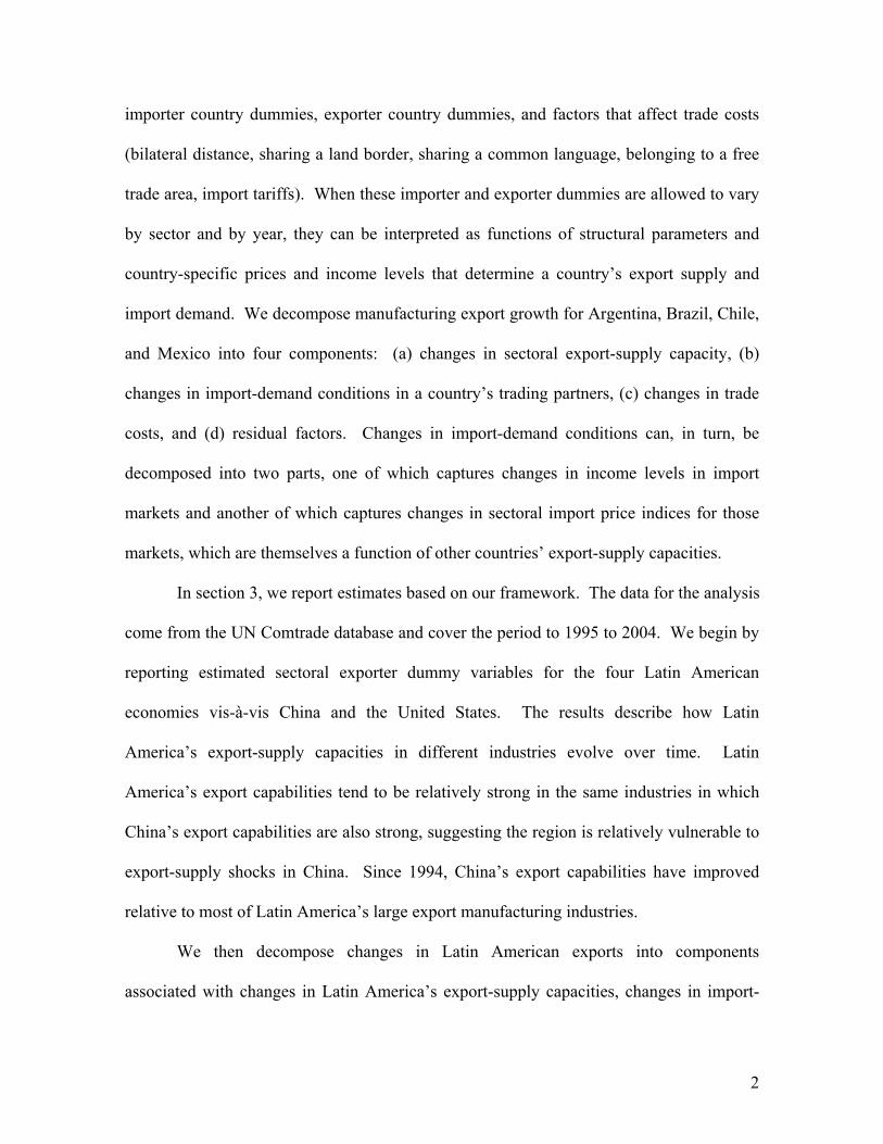
importer country dummies, exporter country dummies, and factors that affect trade costs

(bilateral distance, sharing a land border, sharing a common language, belonging to a free

trade area, import tariffs). When these importer and exporter dummies are allowed to vary

by sector and by year, they can be interpreted as functions of structural parameters and

country-specific prices and income levels that determine a country’s export supply and

import demand. We decompose manufacturing export growth for Argentina, Brazil, Chile,

and Mexico into four components: (a) changes in sectoral export-supply capacity, (b)

changes in import-demand conditions in a country’s trading partners, (c) changes in trade

costs, and (d) residual factors. Changes in import-demand conditions can, in turn, be

decomposed into two parts, one of which captures changes in income levels in import

markets and another of which captures changes in sectoral import price indices for those

markets, which are themselves a function of other countries’ export-supply capacities.

In section 3, we report estimates based on our framework. The data for the analysis

come from the UN Comtrade database and cover the period to 1995 to 2004. We begin by

reporting estimated sectoral exporter dummy variables for the four Latin American

economies vis-à-vis China and the United States. The results describe how Latin

America’s export-supply capacities in different industries evolve over time. Latin

America’s export capabilities tend to be relatively strong in the same industries in which

China’s export capabilities are also strong, suggesting the region is relatively vulnerable to

export-supply shocks in China. Since 1994, China’s export capabilities have improved

relative to most of Latin America’s large export manufacturing industries.

We then decompose changes in Latin American exports into components

associated with changes in Latin America’s export-supply capacities, changes in import-

3

demand conditions, changes in trade costs, and changes in residual factors. While changes

in Latin America’s export-supply capacities have contributed to growth in exports, changes

in Latin America’s import-demand conditions have not, at least since 2000. To explore

why import-demand conditions have not been more favorable, we examine two sources of

negative import-demand shocks: China’s growth in export supply, which may have

lowered import prices in destination markets and diverted import demand away from Latin

America; and the slow down in the growth of the U.S. economy, which may have reduced

growth in demand for the region’s exports. The results suggest that had China’s export-

supply capacity remained constant after 1995, exports for the four Latin American

countries would have been 0.5 to 1.2 percentage points higher during the 1995-2000 period

and 1.1 to 3.1 percentage points higher during the 2000-2004 period. Had U.S. GDP

growth been the same over the 2000-2004 period as it was over the 1995-2000 period,

Latin American exports would have been 0.2 to 1.4 percentage points higher.

The results hold at least three important lessons for policy makers. First, part of the

fluctuation in Latin America’s manufacturing exports appears to be associated with

fluctuations in the U.S. economy. If the U.S. economy continues to recuperate, so too will

demand for Latin American goods on the world market. Since part of Latin America’s

export sluggishness is due to cyclical fluctuations, it is likely to be temporary in nature.

However, this consideration matters more for Mexico than for other countries in the

region. Second, the growth in Latin America’s export-supply capacities has slowed

considerably since the late 1990s. Part of the stagnation in the growth in Latin American

manufacturing exports is attributable to an inability on Latin America’s part to expand the

factors of production that generate export growth. Third, for the time being export growth

4

in China is likely to have adverse consequences on the demand for Latin American

manufacturing exports. For better or worse, Latin America’s most important export

industries (and particularly those of Mexico) are also those in which China’s appears to

have relative strong export capabilities. Given that patterns of national export

specialization tend to change slowly over time, Latin America’s vulnerability to China

appears unlikely to diminish in the near term.

An important caveat to our results is that we focus exclusively on manufacturing

exports. In some countries, notably Brazil and Chile, the growth of China’s economy has

increased demand for commodity exports. The impact of China on Latin America’s

commodity exports does not enter our analysis, making our results partial equilibrium in

nature. The gravity model we develop, which is based on a monopolistic competition

model of trade, would not be appropriate for examining agriculture, mining, or other

sectors that produce primary commodities. Thus, our results do not constitute an analysis

of the aggregate impact of China on Latin American exports.

2. Empirical Specification

2.1 Theory

Consider a standard monopolistic model of international trade, as in Anderson and

van Wincoop (2004) or Feenstra (2004). Let there be J countries and N manufacturing

sectors, where each sector consists of a large number of product varieties. All consumers

have identical Cobb-Douglas preferences over CES sectoral composites of product varieties,

where in each sector n there are In varieties of n produced with country h producing Inh of

these varieties. There are increasing returns to scale in the production of each variety. In

5

equilibrium each variety is produced by a single monopolistically-competitive firm and In is

large, such that the price for each variety is a constant markup over marginal cost. Free entry

drives profits to zero, equating price with average cost.

Consider the variation in product prices across countries. We allow for iceberg

transport costs in shipping goods between countries and for import tariffs. The c.i.f. price of

variety i in sector n produced by country j and sold in country k is then

nninjk nj nk jk

n

P = w t (d )1

γ⎛ ⎞σ⎜ ⎟σ −⎝ ⎠

(1)

where Pinj is the f.o.b. price of product i in sector n manufactured in country j; σn is the

constant elasticity of substitution between any pair of varieties in sector n; wnk is unit

production cost in sector n for exporter j; tnk is one plus the ad valorem tariff in importer k on

imports of n (assumed to be constant across exporters that do not belong to a free trade area

with importer k); djk is distance between exporter j and importer k; and γn is the elasticity of

transportation costs with respect to distance.

Given the elements of the model, total exports of goods in sector n by exporter j to

importer k can be written as,

1nk

1njknjknnjk

nn GPIYX −σσ−μ= , (2)

where μn is the expenditure share on sector n and Gnk is the price index for goods in sector n

in importer k. Hanson and Robertson (2006) show that equation (2) reduces to

( )1 n1[ jk] nn k nj nj jknk

njk 1 nH 1[hk] nnh nh hknkh 1

Y I w (d )X

I w (d )

−σ− γ

−σ− γ

=

μ τ=

⎡ ⎤τ∑ ⎣ ⎦

. (3)

6

where 1[jk] is an indicator variable that takes a value of one if countries j and k belong to a

free trade area and zero otherwise.

Taking logs and regrouping terms in (3) we obtain,

njk n nk nj 1n jk 2n 3 jk njkln X m s ln d 1[ jk] 1[ jk]ln= θ + + +β +β +β τ + ε , (4)

In equation (4), we see that there are four sets of factors that affect country j’s exports to

country k in sector n. The first term captures preference shifters specific to sector n; the

second term captures demand shifters exporter j faces in sector n and importer k (which are a

function of importer k’s income and supply shifters for other countries that also export to

importer k); the third term captures supply shifters in sector n for exporter j (which reflect

exporter j’s production costs and its industrial capacity in the sector); and the fourth through

sixth terms capture trade costs specific to exporter j and importer k associated with bilateral

distance, sharing a common language, sharing a land border, belonging to a free trade area,

and import tariffs. Exporter j’s shipments to importer k would expand if importer k’s income

increases, production costs increase in other countries that supply importer k, exporter j’s

supply capability expands (due to lower production costs or an expanded industrial base), or

trade costs between the two countries decrease.

2.2 Decomposing Export Growth

Using annual data on bilateral trade by sector for a large cross section of countries, we

estimate the parameters in equation (4). We do not need data on the components of mnk or snj.

By estimating equation (4) sector by sector and year by year, we identify the mnk terms by

including importer-specific dummy variables as regressors and the snj terms by including

exporter-specific dummy variables as regressors.

7

Since equation (4) includes a constant term (θn), the estimated coefficients can be

interpreted as deviations from mean industry export or import values. Thus, mnk is the

deviation from sector-n mean import demand for importer k and snj is the deviation from

sector-n mean supply for exporter j. As a practical matter, we do not observe a country’s

exports to itself. Consequently, the country we treat as the excluded category in (4), off

which the constant term is estimated, must be excluded from both the set of export dummies

and the set of import dummies. The interpretation of the constant term is thus the mean trade

value (rather than the mean export or import value) for the excluded country, which in all

regressions we designate as the United States.

The specification in equation (4) is quite general. Restrictions arise only when we

attempt to interpret the importer and exporter dummies. For instance, we have assumed that

within sectors product varieties are identical between countries. Quality may be an important

dimension along which varieties vary, especially between higher-wage and lower-wage

exporters (Schott, 2004; Hummels and Klenow, 2005). Thus, the snj terms may also embody

cross-country differences in the quality of product varieties. When evaluating how these

terms change over time, we need to be mindful that improving quality is an additional means

through which countries can expand their export capabilities. To identify exporter and sector-

specific product quality parameters, we would need to know import quantities (which are

unreported for many countries) and the value of σn for each sector.

For year t, let the OLS estimates of equation (4) be given by

nt nkt njt nt njkt, m , s , , andθ β ε% %% % % . For exposition simplicity, we subsume all variables associated

with trade costs into a single term, denoted by the distance variable. Shipments by exporter j

to importer k in sector n and year t equal

8

s mnt njt nkt njkt ntnjkt jkX e dθ + + +ε β=

% %% % %, (5)

and total exports by exporter j in sector n and year t equal

Hs mnt njt nkt njkt nt

njt jkK 1

X e e dθ + +ε β

== ∑

% %% % %. (6)

From (5) and (6), we can isolate the sources of export growth by country and sector. We

write the distance term compactly as though it were a single variable, whereas in truth we

model trade costs as a function of bilateral distance, sharing a common language, sharing a

land border, belonging to a free trade area (FTA), and import tariffs (which from equation (3)

only appear for country pairs belonging to the same FTA).

One source of export growth is improvement in the supply capability of exporter j in

sector n, relative to the average for all other countries, which is captured by the sectoral

exporter dummy, snjt. The exporter dummy captures in part exporter j’s average comparative

advantage in sector n. A second source of export growth is changes in import demand, which

is a function of national income in an importer country and product prices in the importer,

which are in turn a function of the production costs and industrial capacities of the exporting

countries that supply the importer.

To decompose changes in exports into component parts associated with changes in

export capabilities and changes in demand conditions, rewrite (6) as

s mnjt njkt ntnt nktnjkt nt njt nkt njkt njktjkX e e e e d S M E Dε βθ= ≡ Θ%% % %% . (7)

For years t and t+s, define tst ZZZ −≡Δ + and )ZZ(*5.0Z tst +≡ + . Since Xnjkt is the

product of five terms, there are 60 (5!/2) unique ways to decompose Δ Xnjkt. For any

individual component (Θ, S, M, D, or E), we take the mean across the possible decomposition

terms. Changes in exports for exporter-importer pair jk in sector n are,

9

njk njk njknjkt njt njt nkt

njk njknjkt njkt

X SMDE S MDE M SDE

D SME E SMD

Δ = ΔΘ +Δ Θ + Δ Θ

+ Δ Θ + Δ Θ, (8)

where njkMDEΘ is the mean across the 60 possible orderings of the 5 elements that compose

trade values in (8) and so forth. For exporter j, the change in total exports can be written by

summing across sectors (n) and importers (k) in (8),

njk njkjt njkt njt njt

n k n k

njk njk njknkt njkt njkt

X X ( SMDE S MDE

M SDE D SME E SMD )

Δ = Δ = ΔΘ + Δ Θ∑∑ ∑∑

+ Δ Θ + Δ Θ + Θ. (9)

The first term on the right of (9) is the change in exports for exporter j associated with

changes in mean sectoral trade (designated to be that for the United States), the second term is

the change in exports associated with changes in exporter j’s supply capabilities, the third

term is the change in exports associated with demand conditions in countries than import

from exporter j, the fourth term is the change in exports associated with innovations in trade

costs (or trade-cost elasticities), and the fifth term is residual sources of change in j’s exports.

Equation (9) is the basis for our decomposition results.

2.3 Decomposing Changes in Import-Demand Conditions

Returning to equation (3), it is apparent that a further decomposition of import-

demand conditions facing country j is possible. In theory,

n n n

H1 1[hk](1 )

nk k nh nh nh hkh 1

m ln Y ln I w d−σ − −σ β

=

⎛ ⎞= − τ⎜ ⎟

⎝ ⎠∑ . (10)

Thus, exporter j faces import-demand shocks due to changes in income and import prices in

its trading partners, where import prices are a function of export-supply conditions in the

countries that also export to country j’s trading partners. One might consider estimating (4)

10

subject to the constraint in (10). However, there are practical difficulties in imposing such a

constraint. As is well known, there is zero trade at the sectoral level between many country

pairs, especially in pairs involving a developing country. Tenreyro and Santos (2005)

propose a Poisson pseudo-maximum likelihood (PML) estimator to deal with zero

observations in the gravity model. In our application, this approach is subject to an

incidental-parameters problem (Wooldridge, 2002). While in a Poisson model it is

straightforward to control for the presence of unobserved fixed effects, it is difficult in this

and many other nonlinear settings to obtain consistent estimates of these effects. Since, at the

sectoral level, most exporters trade with no more than a few dozen countries, PML estimates

of exporter and importer country dummies may be inconsistent.

Our approach is to estimate equation (4) using OLS for a set of medium to large

exporters (OECD countries plus larger developing countries, which account for

approximately 90% of world manufacturing exports) and larger importers (countries that

account for approximately 90% of world manufacturing imports). For bilateral trade between

larger countries, there are relatively few zero trade values. However, since we do not account

explicitly for zero bilateral trade in the data, we are left with unresolved concerns about the

consistency of the parameter estimates.1

Using (10), we modify (9) to decompose demand shifters that are specific to importer

k (say, the United States) into a component associated with GDP in country k (e.g., U.S.

business-cycle conditions) and a component associated with the import-price index in

importer k, which is in turn a function of trade-cost-weighted export-supply shifters among

the countries that export to importer k. In this framework, we can identify the contribution of

1 Choosing larger countries may subject the specification to selection bias. See Helpman, Melitz, and Rubinstein (2004).

11

changes in, say, China’s export capacity to changes in other countries’ demand for imports.

We can also perform counterfactual decompositions of export growth for Latin American

countries (or other countries) in which we assess how export growth in the country would

have been different if China’s export dummies had remain unchanged (which then would

have increased global demand for other countries’ goods) or if U.S. GDP growth had remain

unchanged (which would have affected its import demand).

These counterfactual decompositions are not general-equilibrium in nature. Altering

China’s growth in export supply would affect the export supply of all other countries, not just

Latin America. Thus, the counterfactual decompositions we construct are likely to

overestimate the impact of export growth in China on Latin American manufacturing exports.

Our results are perhaps best seen as upper bounds of the possible impact of China on Latin

America’s manufacturing sector. Similar qualifications apply to the counterfactual

decomposition in which we constrain US GDP growth to be constant.

3. Empirical Results

The data for the analysis come from the UN Comtrade database and cover

manufacturing imports over the period 1995 to 2004. We examine bilateral trade at the

four-digit harmonized system (HS) level. We limit the sample to the top 40 export

industries in Brazil and Mexico and the top 20 export industries in Argentina and Chile.2

This sample of industries accounts for over 85% of manufacturing exports in each of the

four countries. We estimate the gravity equation in (4) on a year-by-year basis, allowing

coefficients on exporter country dummies, importer country dummies, and distance to vary

by sector and year. The output from the regression exercise is for each sector a panel of 2 In later work, we will expand the sample to include more industries and countries.

12

exporter and importer country dummy variables, trade-cost coefficients, intercepts, and

residuals. The country dummies are the deviation from the U.S. sectoral mean trade by

year. For these coefficients to be comparable across time, the conditioning set for a given

sector (i.e., the set of comparison countries) must be constant across time. For each sector,

we limit the sample to bilateral trading partners that have positive trade in every year

during the sample period (by only including consistent trading partners in the sample we

introduce another potential source of selection bias into the estimation).

3.1 Estimates of Sectoral Export Supply Capacities

The regression results for equation (4) involve a large amount of output. In each

year, we estimate over 10,000 country-sector exporter coefficients, over 5,000 country-

sector importer coefficients, and over 90 trade-cost coefficients. To summarize exporter

and import dummies compactly, Figures 1a and 1b plot kernel densities for the sector-

country exporter and importer coefficients (where the densities are weighted by sector-

country exports or imports). Figure 1a shows that most exporter coefficients are negative,

consistent with sectoral exports for most countries being below the United States. Over the

sample period, the distribution of exporter coefficients shifts to the right, suggesting other

countries are catching up to the United States. The figure indicates by vertical lines

weighted mean values for Mexico’s exporter coefficients in 1994 (equal to -3.9), 2000

(equal to -2.6), and 2004 (equal to -2.1), which rise in value over time relative to the

overall distribution of exporter coefficients, suggesting Mexico’s export-supply capacity

improves relative to other countries over the sample period. Mean exporter coefficients

fall over time for Argentina (-0.21 in 1994 and -1.26 in 2004), Brazil (-0.12 in 1994 and -

13

0.68 in 2004), and Chile (0.29 in 1994 and -0.34 in 2004). Thus, among the four Latin

American countries, only Mexico shows consistent average improvement in its

manufacturing export capacity. This could reflect the importance of commodity exports

for the countries other than Mexico. A commodity export boom could diminish

manufacturing export capacity by driving up the price of immobile factors of production,

such as labor and land. In Figure 1b, most importer coefficients are also negative, again

indicating sectoral trade values for most countries are below those for the United States.

To provide further detail on the coefficient estimates, an appendix reports mean

exporter and importer coefficients by country (across sectors and years) and the fraction of

coefficient estimates that are statistically significant.3 For the large majority of countries,

exporter and importer coefficients are precisely estimated. Further detail on the coefficient

estimates is available in Table 1, which reports average parameter estimates on the trade-

cost variables. For the most part, the results align with previous literature (see Anderson

and van Wincoop, 2004). While coefficients on distance and being in an FTA fluctuate

mildly over the period, common language and adjacency show uneven downward trends.

The coefficient on the tariff-FTA interaction increases markedly after 2000. Since 2000 is

the dividing point between a period of global economic expansion and a period of global

economic stagnation, the results may indicate that business cycles may affect substitution

elasticities (or at least gravity model estimates of these elasticities).

Of primary interest is how Latin America’s export-supply capacities compare to

those of China and to import-demand conditions in the United States. Figures 2a-2d plot

export coefficients for the four Latin American countries against the constant terms in the

3 The current appendix gives results for 40 of the 90 industries in the sample. We will expand the coverage of the appendix in later versions of the paper.

14

regressions, which represent mean sectoral trade values for the United States.

Observations are weighted by each country’s sectoral shares of annual manufacturing

exports. The figures show a negative relation for all countries except Chile (-0.11 for

Argentina, -0.64 for Brazil, 0.27 for Chile, and -0.28 for Mexico, all of which are

statistically significant), suggesting that most Latin American countries tend to have

stronger exports in sectors in which the United States has lower levels of trade. Figures

3a-3d plot annual changes in Latin America’s export coefficients against annual changes in

the constant terms, which are changes in mean U.S. sectoral trade. Again, for each country

except Chile, there is a negative correlation between the two sets of coefficients (-0.29 for

Argentina, -0.43 for Brazil, 0.11 for Chile, and -0.69 for Mexico, all statistically

significant). Sectors in which Latin America shows most improvement in export-supply

capacity tend to be those in which the United States shows weaker increases in trade.

Figures 4a-4d plot exporter coefficients for the four countries against China over

the sample period (again using each country’s sectoral shares of annual manufacturing

exports as weights). For all countries, there is a positive correlation between the two sets

of exporter coefficients (0.34 for Argentina, 0.35 for Brazil, 0.49 for Chile, and 0.32 for

Mexico, all statistically significant). Sectors in which Latin America has a relatively

strong export-supply capacity tend to be those in which China’s export capacity is also

strong. Since exporter coefficients are expressed as deviations from U.S. sectoral means,

the positive correlation between exporter coefficients for Latin America and China is not

simply a statistical artifact of the data (as would be the case, for instance, if we were

comparing mean sectoral exports in Latin America and China). Figures 4a-4d show that,

15

conditional on sectoral trade values for the United States, China tends to have higher

exports in Latin America’s larger manufacturing export industries.

Figures 5a-5d plot annual changes in export coefficients for Latin America against

those for China (weighted by each country’s annual industry export shares). For all

countries except Chile, the correlation is positive (0.51 for Argentina, 0.22 for Brazil, -0.04

for Chile, and 0.74 for Mexico, all except Chile are statistically significant). This suggests

that industries in which China’s export supply capacities are strengthening also tend to be

those in which Latin America’s export capacities are strengthening. Since the plotted

values are changes in deviations from U.S. industry means (and not changes in the means

themselves), the correlations are not an artifact of the data.

To compare the export capabilities of Latin America and China for individual

sectors, Figures 6a-6d plot export coefficients in China against the 16 largest

manufacturing export sectors in each Latin American country (which over the sample

period account for 85% of Argentina’s manufacturing exports, 70% of Brazil’s

manufacturing exports, 90% of Chile’s manufacturing exports, and 75% of Mexico’s

manufacturing exports). Note first that the identities of the industries vary considerably

across countries, indicating that there is variation across Latin American countries in the

sectors in which national exports are concentrated. This fact makes the positive

correlations between China and Latin America’s export supply capacities in Figures 4 and

5 all the more remarkable. Despite the diversity of industries represented, China tends to

be strong in many or most of the larger export industries accounted for by Argentina,

Brazil, and Mexico. For Argentina, China’s export supply capacities show relative

16

improvement in 7 of the 14 industries for which we have estimates for China.4 For Brazil,

China’s export supply capacities show relative improvement in 10 of the 15 industries for

which we have estimates for China. For Chile, China’s export supply capacities show

relative improvement in 5 of the 13 industries for which we have estimates for China. And

for Mexico, China’s export supply capacities show relative improvement in 12 of the 16

industries. The evidence in Figure 6 suggests that among the four countries Chile is least

exposed and Mexico is most exposed to export supply shocks from China. Results we

report next will be consistent with this finding.

3.2 Decomposing Manufacturing Export Growth

Our next exercise involves the decomposition of export growth for the four Latin

American countries into changes in export-supply capacities, changes in import-demand

conditions, and changes in other components, as proposed in equation (9). Table 3 reports

the total change in manufacturing exports for Argentina, Brazil, Chile, and Mexico over

two time periods, 1995-2000 and 2000-2004. The reported change in trade is the total

change in trade values (divided by the number of years in the subperiod), normalized by

the average of trade values in the beginning and end period. Thus, for instance, Table 3

shows that manufacturing exports in Mexico grew by an annual average of 16.5% over

1995-2000 and 2.4% over 2000-2004.

The results in Table 3 are for a restricted set of industries. When we include the

full sample of manufacturing industries, we tend to obtain implausibly large values for

individual decomposition terms in food products, mineral processing, or other industries

4 Sectors in which we do not have estimates of export supply capacities for China are those in which China does not export to at least one country in all years covered in the sample (1995-2004).

17

associated with the processing of primary commodities for Brazil and Chile (but not for

Argentina or Mexico). As a crude way to address this problem, we limit the results we

report in this paper to those for HS two-digit industries 80 to 99, which consists of metal

products, machinery, electronics, transportation equipment, and industrial equipment, none

of which are intensive in natural resources or primary commodities.5 Even with this

sample restriction, the decomposition terms for Brazil are too large to be credible.

The first column of Table 3 shows that in all countries manufacturing export

growth was slower after 2000 than before, with Argentina exhibiting the largest decline

(during a period that follows the country’s abandonment of its currency board and ensuing

economic turmoil) and Mexico showing the next largest decline.

Two other patterns in Table 3 are worthy of note. One is that in column (2) for all

countries the contribution of the exporter coefficients to export growth is larger before

2000 than after. This suggests that in Latin America a slow down in the growth of

manufacturing export supply capacity contributed to the slow down in manufacturing

export growth. While the decomposition does not isolate the source of the slowing in

Latin America’s export supply capacity, one obvious source would be constraints on

manufacturing growth. These constraints are likely to vary by country. In Brazil and

Chile, which have enjoyed export-driven booms in commodity production, constraints on

manufacturing growth may come from other sectors of the economy enjoying relative price

increases and as a result expanding more rapidly, absorbing resources that would have

otherwise gone into manufacturing. In Mexico, which has not enjoyed a similar

5 The four-digit industries in HS two-digit industries 80 to 99 are tin and articles thereof, base metals and articles thereof, tools, miscellaneous articles of base metal, boilers and machinery, electrical and electronic equipment, railway equipment, motor vehicles, aircraft, ships, optical equipment, clocks and watches, musical instruments, arms and ammunition, furniture, toys and games, miscellaneous manufactured articles, works of art, and other commodities.

18

commodity boom, domestic factors may be the primary obstacle to growth. These may

include relatively high energy prices, poor telecommunications infrastructure, and slow

growth in the supply of skilled labor, among other possible factors.

A second notable pattern in Table 3 is that mean US sectoral trade contributes

much less to export growth in Latin America after 2000 than before. There are several

possible explanations for this. One is that the slowing of the US. economy after 2000

resulted in slower growth in U.S. demand for imports, thereby contributing to slower

export growth in Latin America. If the sluggishness of the U.S. economy is the primary

source of the slowing in U.S. demand for Latin America’s exports, this shock is likely to

be temporary. As the U.S. economy continues to recuperate, demand for Latin America’s

exports would likely grow. A second possibility is that China’s continued export

expansion has lowered relative prices for manufacturing goods and displaced exports from

other countries, including those from Latin America, in the U.S. market. A China-related

negative demand shock for Latin American manufacturing exports would be of greater

concern than a negative demand shock associated with slow growth in the U.S. economy,

for China’s export strength in manufacturing is likely to persist. In the next section, we

explore these two options in more detail.

3.3 Counterfactual Decompositions

The results in Table 3 provide a summary of how Latin American exports have

grown but they do not reveal why they have grown. To explore this issue, we apply

insights derived from equation (10). In Table 4, we explore how Latin America’s export

growth might have differed had the U.S. economy not slowed down after 2000. We

19

impose the assumption that U.S. GDP growth over 2000 to 2004 (2.6%) was the same as

that over 1995 to 2000 (3.2%). Returning to (9), we perform the following counterfactual

calculation:

s mnjt njkt ntnt nkt nktnjkt nt njt nkt njkt njktjkˆX e e e e d S M E Dε βθ +π= ≡ Θ

%% % %% , (11)

in which we set πnkt equal to 0.024 (4*0.006) if k equals the United States and t equals

2004, and zero otherwise. This has the effect of inflating the import-demand coefficient

for the United States in 2004 to what it would have been had the U.S. economy grown by

the same rate after 2000 as it had before (and no other changes occurred in the global

economy). We then use (11) to estimate counterfactual export growth in the four Latin

American countries over 2000-2004, in which we replace nktMΔ with nnkktM̂Δ .

It is important to recognize that the counterfactual estimation of Latin American

export growth in Table 4 is not a general-equilibrium exercise. Since the United States is a

large country, stronger U.S. economic growth (due, say, to higher levels of Hicks neutral

technological change) would have likely affected the global demand for goods and therefore

global factor demands, generating changes in factor prices in U.S. trading partners, including

Latin America. In the counterfactual calculations we report, we assume away such feedback

effects from import demand into factor prices. Since higher demand for Latin American

exports would have likely increased production costs in the country and the relative price of

Latin American exports, the counterfactual export growth we report likely overstates what

would have occurred in actuality

The results in Table 4 suggest that had U.S. GDP growth not decelerated after 2000,

over 2000-2004 Argentine exports would have grown by 0.2% more, Brazilian exports would

have grown by 0.8% more, Chilean exports would have grown by 0.7% more, and Mexican

20

exports would have grown by 1.4% more. In performing this exercise, we impose the unitary

coefficients on the variables on the right of equation (10). The results suggest that had the

U.S. economy not slowed down in the early 2000s, only in Mexico would export growth

been more than nominally higher than it was. That the U.S. slow down matters more for

Mexico is not surprising. The United States is a much larger trading partner for Mexico

than for the countries of South America. What perhaps is surprising is that changes in U.S.

GDP appear to matter so little for Latin American exports overall.

To evaluate the impact of China’s export growth on Latin America, we again utilize

(10). We impose the assumption that China’s export coefficients remain unchanged from

1995 forwards. Following (10), this would have the effect of raising the import-price

index in importing countries, leading to an overall increase in their importer coefficient.

For country k, we redefine the change in importer coefficient in (11) to be,

nt nt nt ntnht nc0 nht ncts s s snkt hk hk hk hk

h c h cln e d e d ln e d e dβ β β β

≠ ≠

⎛ ⎞ ⎛ ⎞π = + − +∑ ∑⎜ ⎟ ⎜ ⎟

⎝ ⎠ ⎝ ⎠

% % % %% % % % , (12)

where h=c indicates China and nc0s% indicates China’s exporter coefficient in sector n in the

initial period. Thus, (12) shows how the importer coefficient for country k would have

differed in year t had China’s exporter coefficients remain unchanged from the initial year.

Again, it is important to recognize that this is not a general-equilibrium exercise.

The results in Table 4 suggest that had China’s export-supply capacity not changed

over the sample period, Argentina’s annual average export growth would have been 0.4

percentage points higher over 1995-2000 and 1.1 percentage points higher over 2000-2004,

Brazil’s annual average export growth would have been 0.7 percentage points higher over

1995-2000 and 1.4 percentage points higher over 2000-2004, Chile’s annual average

21

export growth would have been 0.8 percentage points higher over 1995-2000 and 2.3

percentage points higher over 2000-2004, and Mexico’s annual average export growth

would have been 1.2 percentage points higher over 1995-2000 and 3.1 percentage points

higher over 2000-2004. Naturally, the effects are larger in the latter time period, as the

impact of holding China’s export supply capacities constant cumulates over time.

Consistent with Figures 4-6, of the four countries Mexico appears to be the most exposed

to export competition from China. This owes to the fact that China’s strong export

industries overlap more with Mexico than with the other countries of Latin America.

Interestingly, the impact on Latin American exports of China’s export-capacity

growth is two to five times as large as the impact of the U.S. economic slowdown. While

it may be reasonable to view sluggish U.S. growth as a temporary shock, the same does not

hold for China’s export growth. Thus, only a small part of the recent slow down in Latin

American export growth appears associated with transitory business cycle factors.

Comparing the results in Tables 3 and 4, the estimated impact of China’s growth on

Latin America is small relative to the impact of changes in the countries’ export-supply

capacities, distance coefficients, or residual factors. While China’s performance clearly

seems to affect Latin America, other factors matter more.

4. Discussion

In this paper, we use the gravity model of trade to decompose Latin America’s

export growth into components associated with export-supply capacity, import-demand

conditions, and other factors. We apply the framework to Argentina, Brazil, Chile, and

Mexico. There are three main findings. First, since the mid 1990s export-supply

22

capacities in Mexico, but not the other countries, have improved relative to the rest of the

world. Commodity booms in Brazil and Chile and economic crisis in Argentina may

account for the apparent decrease in the countries’ manufacturing export supply

capabilities. Second, Argentina, Brazil, and Mexico are relatively exposed to export-

supply shocks from China, with Mexico being the most exposed. Industries in which

Mexico has strong export capabilities are also those in which China’s capabilities are

strong, and in most industries China’s capabilities improve over time relative to Mexico.

Had China’s export-supply capacities remained constant from 1994 onward, Latin

America’s annual export growth rate would have been up to 0.4 to 1.4 percentage point

higher during the late 1990s and 1.1 to 3.1 percentage points higher during the early 2000s.

Third, while changes in Latin America’s export-supply capacities have contributed

positively to the country’s export growth, changes in U.S. import demand in Latin

America’s key export industries have not. Latin America’s exports are concentrated in

sectors in which the United States has shown relatively weak growth in trade. Had U.S.

GDP grown at the same rate from 2000 to 2004 as it had in the late 1990s, Latin America’s

annual export growth rate would have been up to 0.2 to 1.4 percentage points higher.

There are several important caveats to our results. Our framework and analysis are

confined to manufacturing industries and the decomposition of export growth is confined

to a subset of manufacturing industries (mainly industrial machinery, electronics, and

transportation equipment). There may be important consequences of China or U.S.

business cycles for Latin America’s commodity trade, which we do not capture. The

counterfactual decompositions of export growth that we report do not account for general-

equilibrium effects. There could be feedbacks from a slowdown in China’s export growth

23

or an increase in U.S. GDP growth that would cause us to overstate the growth

consequences of such shocks for Latin America. There are also concerns about the

consistency of the coefficient estimates, due to the fact that we do not account for why

there is zero trade between some countries.

The results have a number of important lessons for policy makers. Of the four

countries, Mexico appears to be most exposed to import-demand shocks associated with

U.S. aggregate demand and competition from China. Given that patterns of industrial

specialization tend to change slowly over time, Mexico’s exposure to China is unlikely to

change in the short to medium run. Yet, while negative, the effects of China’s growth on

Latin America’s manufacturing exports are not as large as many appear to believe.

Domestic constraints on manufacturing appear to be a more important factor limiting

export growth in all four of the countries examined.

24

References

Anderson, James E. and Van Wincoop, Eric. “Gravity with Gravitas: A Solution to the Border Puzzle.” American Economic Review, March 2003.

Anderson, James E. and Van Wincoop, Eric. “Trade Costs.” Journal of Economic

Literature, September 2004. Devlin, Robert, Antoni Estevadeordal, and Andres Rodriguez. 2005. The Emergence of

China: Opportunities and Challenges for Latin America and the Caribbean. Washington, DC: Inter-American Development Bank.

Eichengreen, Barry, and Hui Tong. 2005. “Is China’s FDI Coming at the Expense of

Other Countries?” NBER Working Paper No. 11335. Feenstra, Robert C. Advanced International Trade: Theory and Evidence. Princeton:

Princeton University Press, 2003. Feenstra, Robert C.; Lipsey, Robert and Bowen, Charles. “World Trade Flows, 1970-1992,

with Production and Tariff Data.” National Bureau of Economic Research (Cambridge, MA) Working Paper No. 5910, January 1997.

Feenstra, Robert C., Robert Lipsey, Haiyan Deng, Alyson C. Ma, and Hengyong Mo.

2005. “World Trade Flows: 1962-2000.” NBER Working Paper No. 11040. Fujita, Masahisa, Paul Krugman, and Anthony Venables. 1999. The Spatial Economy:

Cities, Regions, and International Trade. Cambridge, MA: MIT Press. Hanson, Gordon, and Chong Xiang. “The Home Market Effect and Bilateral Trade

Patterns,” American Economic Review, September 2004, 94: 1108-1129. Hanson, Gordon, and Raymond Robertson. “A Gravity Framework for Decomposing

Demand and Supply Shocks to Trade.” Mimeo, UCSD and Macalaster College. Harrigan, James. 1995. "Factor Endowments and the International Location of Production:

Econometric Evidence For the OECD, 1970-1985." Journal of International Economics 39: 123-141.

Harrigan, James. 1997. "Technology, Factor Supplies, and International Specialization:

Estimating the Neoclassical Model." American Economic Review 87: 475-494. Head, Keith and Ries, John. “Increasing Returns versus National Product Differentiation as

an Explanation for the Pattern of US-Canada Trade.” American Economic Review, September 2001, 91(4), pp. 858-76.

25

Head, Keith, and Mayer, Theiry. “The Empirics of Agglomeration and Trade.” In J. Vernon Henderson and Jacque Thisse, eds., Handbook of Regional and Urban Economics, Amsterdam: North Holland, 2004.

Helpman, Elhanan, Marc J. Melitz, and Yona Rubinstein. 2004. “Trading Partners and

Trading Volumes,” mimeo, Harvard University. Hummels, David. “Towards a Geography of Trade Costs.” Mimeo, University of Chicago,

1999. Hummels, David, and Peter Klenow. 2005. “The Variety and Quality of a Nation’s

Exports.” American Economic Review, 95: 704-723. Leamer, Edward E. Sources of International Comparative Advantage: Theory and

Evidence. Cambridge, MA: MIT Press, 1984. Lopez Cordoba, Ernesto, Alejandro Micco, and Danielken Molina. 2005. “Howe

Sensitive Are Latin American Exports to Chinese Competition in the U.S. Market?” Mimeo, Inter-American Development Bank.

Redding, Stephen and Venables, Anthony J. “Geography and Export Performance:

External Market Access and Internal Supply Capacity.” NBER Working Paper No. 9637, April 2003.

Redding, Stephen and Venables, Anthony J. “Economic Geography and Global

Development.” Journal of International Economics, January 2004. Santos Silva, J.M.C., and Silvana Tenreryo. 2005. “The Log of Gravity.” The Review of

Economics and Statistics, forthcoming. Schott, Peter. 2004. “Across Product versus within Product Specialization in International

Trade.” Quarterly Journal of Economics, May 119(2): 647-678. Wooldridge, Jeffrey M. 2002. Econometric Analysis of Cross Section and Panel Data.

Cambridge, MA: MIT Press.

26

Appendix A: Average Exporter Coefficients (for countries that do not appear as importers)

Country Exporter

Coefficient % Significant Angola 0.776 62.50 United Arab Emirates 1.135 98.70 Bangladesh 0.900 70.17 Bulgaria -3.292 99.40 Cote d'Ivoire 0.939 89.12 Cameroon -0.009 60.00 Dominican Republic -4.061 91.46 Gabon -0.268 70.00 Honduras -2.187 100.00 Iran, Islamic Rep. 0.935 87.26 Kuwait 0.884 83.28 Sri Lanka -1.621 88.38 Nigeria 0.955 67.45 Pakistan -1.363 87.49 Philippines -2.544 97.75 Qatar 0.682 76.47 Saudi Arabia 1.599 85.67 Thailand -2.481 84.52 Trinidad and Tobago -2.842 96.40 Taiwan, China -1.200 92.65

Appendix B: Average Country Importer and Exporter Coefficients (for countries that appear as exporters and importers)

Country Importer

Coefficient % SignificantExporter

Coefficient %

Significant

Argentina -3.121 97.94 -2.466 98.60 Australia -1.925 96.59 -2.380 98.22 Austria -4.104 100.00 -3.935 100.00 Brazil -2.173 98.67 -1.662 99.47 Canada -2.148 99.06 -2.291 99.77 Switzerland -3.924 99.81 -3.835 99.72 Chile -3.222 98.19 -4.654 98.46 China -1.440 93.59 0.367 83.13 Colombia -3.949 99.88 0.211 98.84 Costa Rica -5.670 100.00 -3.446 99.94 Czech Republic -4.522 99.98 -3.767 99.12 Germany -1.554 93.57 -0.196 68.49 Denmark -4.165 100.00 -3.090 99.22 Algeria -5.204 100.00 -0.790 75.00

27

Ecuador -4.565 99.98 -0.536 89.43 Egypt, Arab Rep. -4.871 100.00 -1.173 97.94 Spain -2.886 99.38 -2.052 96.06 Finland -4.024 100.00 -2.836 98.88 France -2.306 99.52 -1.539 91.75 United Kingdom -1.688 94.94 -1.679 96.64 Greece -4.026 100.00 -3.368 97.11 Guatemala -5.376 100.00 -1.883 99.63 Hong Kong, China -1.829 94.40 -1.385 93.18 Hungary -4.096 100.00 -3.835 98.22 Indonesia -3.252 99.06 -0.835 78.45 India -3.559 99.97 -1.906 90.43 Ireland -3.674 100.00 -3.349 98.63 Iceland -6.030 100.00 -8.117 100.00 Israel -3.420 99.35 -3.679 100.00 Italy -2.482 99.45 -1.220 83.48 Japan -1.351 95.95 0.332 78.57 Korea, Rep. -1.840 99.14 -1.135 82.87 Morocco -4.878 100.00 -2.615 94.57 Mexico -2.592 99.92 -2.129 95.85 Malaysia -1.860 98.59 -1.599 91.67 Netherlands -2.413 99.85 -3.027 97.12 Norway -3.908 99.51 0.533 98.99 New Zealand -3.012 99.02 -3.921 99.40 Oman -4.489 100.00 0.628 79.77 Peru -4.377 100.00 -1.022 99.59 Poland -3.677 99.78 -2.933 98.41 Portugal -4.197 99.84 -3.368 93.01 Romania -4.885 100.00 -2.402 92.13 Singapore -1.392 97.32 -1.679 93.96 El Salvador -5.676 100.00 -1.877 95.65 Sweden -3.366 100.00 -2.349 99.53 Tunisia -6.049 100.00 -2.583 93.98 Turkey -3.510 99.31 -1.092 91.70 Venezuela -3.924 99.48 -0.254 86.11 South Africa -2.897 99.52 -3.531 99.84

28

Appendix C: HS Industry Code Descriptions

4 Digit HS Description 901 Coffee; Coffee Husks Etc; Substitutes With Coffee 2203 Beer Made From Malt 2709 Crude Oil From Petroleum And Bituminous Minerals 2710 Oil (Not Crude) From Petrol & Bitum Mineral Etc. 6109 T-Shirts, Singlets, Tank Tops Etc, Knit Or Crochet 6110 Sweaters, Pullovers, Vests Etc, Knit Or Crocheted 6203 Women's Or Girls' Overcoats Etc, Not Knit Or Croch 6204 Men's Or Boys' Suits, Ensembles Etc, Not Knit Etc 8407 Spark-Ignition Recip Or Rotary Int Comb Piston Eng 8409 Parts For Engines Of Heading 8407 Or 8408 8414 Air Or Vac Pumps, Compr & Fans; Hoods & Fans; Pts 8415 Air Conditioning Machines (Temp & Hum Change), Pts 8418 Refrigerators, Freezers Etc; Heat Pumps Nesoi, Pts 8471 Automatic Data Process Machines; Magn Reader Etc 8473 Parts Etc For Typewriters & Other Office Machines 8481 Taps, Cocks, Valves Etc For Pipes, Tanks Etc, Pts 8501 Electric Motors And Generators (No Sets) 8504 Elec Trans, Static Conv & Induct, Adp Pwr Supp, Pt 8512 Electric Light Etc Equip; Windsh Wipers Etc, Parts 8516 Elec Water, Space & Soil Heaters; Hair Etc Dry, Pt 8517 Electric Apparatus For Line Telephony Etc, Parts 8518 Microphones; Loudspeakers; Sound Amplifier Etc, Pt 8525 Trans Appar For Radiotele Etc; Tv Camera & Rec 8527 Reception Apparatus For Radiotelephony Etc 8528 Tv Recvrs, Incl Video Monitors & Projectors 8529 Parts For Television, Radio And Radar Apparatus 8536 Electrical Apparatus For Switching Etc, Nov 1000 V 8537 Boards, Panels Etc Elec Switch And N/C Appar Etc. 8541 Semiconductor Devices; Light-Emit Diodes Etc, Pts 8542 Electronic Integrated Circuits & Microassembl, Pts 8544 Insulated Wire, Cable Etc; Opt Sheath Fib Cables 8703 Motor Cars & Vehicles For Transporting Persons 8704 Motor Vehicles For Transport Of Goods 8708 Parts & Access For Motor Vehicles (Head 8701-8705) 9018 Medical, Surgical, Dental Or Vet Inst, No Elec, Pt 9029 Revolution & Production Count, Taximeters Etc, Pts 9032 Automatic Regulating Or Control Instruments; Parts 9401 Seats (Except Barber, Dental, Etc), And Parts 9403 Furniture Nesoi And Parts Thereof 9405 Lamps & Lighting Fittings & Parts Etc Nesoi

29

Table 1: Average Coefficient Estimates on Trade Cost Variables

Year ln(Distance) Common Language Adjacency FTA FTA*ln(1+Tariff)

1995 -1.118 0.652 0.519 0.045 7.964 1996 -1.121 0.640 0.402 0.121 5.757 1997 -1.115 0.531 0.370 0.065 7.112 1998 -1.076 0.573 0.461 0.016 7.490 1999 -1.076 0.542 0.382 0.028 8.540 2000 -1.111 0.532 0.255 -0.074 11.396 2001 -1.086 0.493 0.239 0.001 16.854 2002 -1.049 0.545 0.348 0.165 20.709 2003 -1.063 0.479 0.299 0.184 22.771 2004 -1.118 0.497 0.207 0.128 13.804

Notes: Coefficient estimates are expressed as trade-value-weighted means for manufacturing industries.

30

Table 2a: Industry Shares of Manufacturing Exports for Mexico

HS Industry HS Industry Share of Mexican

Manufacturing Exports Internal combustion engine parts 8409 0.0106 Valves 8481 0.0115 Medical instruments 9018 0.0116 Automatic regulating equipment 9032 0.0139 Radio and TV parts 8529 0.0141 Women's and girl's dresses 6204 0.0147 Electric motors 8501 0.0156 Men's and boy's suits 6203 0.0183 Radio receivers 8527 0.0203 Telephone apparatus 8517 0.0205 Electric transformers 8504 0.0206 Electric switches 8536 0.0226 Internal combustion engines 8407 0.0236 Parts for office machines 8473 0.0248 Seats 9401 0.0278 Radios and TV transmitters 8525 0.0305 Motor vehicle parts 8708 0.0534 TV receivers 8528 0.0558 Motor vehicles for transporting goods 8704 0.0579 Insulated wire and cable 8544 0.0642 Computers 8471 0.0648 Motor vehicles for transporting people 8703 0.1463 Notes: This table shows the share of Mexican manufacturing exports for the industries that account for an average of 75% of Mexico’s total exports over the sample period (1995-2004).

Tables 2b-2d for Argentina, Brazil, and Chile (to be added)

31

Table 3: Decomposing Latin American Export Growth, 1995-2004 Decomposition of Export Growth Component of Growth Associated with Change in: Growth in Manufacturing Exporter Importer Mean Trade-Cost Residual

Period Exports Coefficients Coefficients US Trade Coefficients Factors

Argentina 1995-2000 0.081 0.820 -1.249 0.247 0.692 -0.428

2000-2004 -0.045 0.098 -0.088 0.075 -0.072 -0.057

Brazil 1995-2000 0.130 20.162 -0.111 50.305 -70.172 -0.054

2000-2004 0.111 1.787 -0.042 -4.587 2.924 0.029

Chile 1995-2000 0.071 0.402 -0.007 -0.091 0.323 -0.556

2000-2004 0.053 0.146 -0.016 -0.099 0.005 0.017

Mexico 1995-2000 0.165 0.475 -0.018 0.213 -0.184 -0.322

2000-2004 0.024 0.227 0.007 -0.189 0.154 -0.175

Notes: This table uses equation (9) to decompose annual average growth in a country’s manufacturing exports into components associated with changes in sectoral importer coefficients in a country’s trading partners, changes in a country’s sectoral exporter coefficients, changes in mean U.S. sectoral trade, changes in trade costs (log distance, common language, adjacency, FTAs, tariffs), and changes in residual factors. These preliminary results are limited to four-digit industries in HS two-digit industries 80 to 99 (tin and articles thereof, base metals and articles thereof, tools, miscellaneous articles of base metal, boilers and machinery, electrical and electronic equipment, railway equipment, motor vehicles, aircraft, ships, optical equipment, clocks and watches, musical instruments, arms and ammunition, furniture, toys and games, miscellaneous manufactured articles, works of art, other commodities).

32

Table 4: Counterfactual Decompositions of Latin American Export Growth

Counterfactual Growth in Manufacturing Exports Actual Growth in

Period Manufacturing Exports

Exporter Coefficients in China Constant over Time

US GDP Growth 2000-2004 =1995-2000

Argentina 1995-2000 0.081 0.085 --

2000-2004 -0.045 -0.034 -0.043

Brazil 1995-2000 0.130 0.137 --

2000-2004 0.111 0.125 0.119

Chile 1995-2000 0.071 0.079 --

2000-2004 0.053 0.076 0.060

Mexico 1995-2000 0.165 0.177 --

2000-2004 0.024 0.055 0.038 Notes: This table reports actual and counterfactual export growth in Latin American countries based on two scenarios: U.S. GDP growth over 2000-2004 equals that for 1995-2000, and China’s export-supply capacity remains constant over the sample period (1995 to 2004) at levels equal to 1995 values.

33

D

ensi

ty

Exporter Coefficients

1995 2000 2004

-15 -10 -5 0 5

0

.1

.2

.3

Figure 1a: Estimated Sector-Country Exporter Coefficients, Selected Years

Den

sity

Importer Coefficients

1995 2000 2004

-10 -5 0 5

0

.2

.4

Figure 1b: Estimated Sector-Country Importer Coefficients, Selected Years

34

(deviations from US industry means)

Arg

entin

a E

xpor

ter C

oeffi

cien

t

USA Coefficient10 20 30 40

-10

-5

0

5

Figure 2a: Sectoral Export Coefficients for Argentina and US Sectoral Trade


Bra

zil E

xpor

ter C

oeffi

cien

t

USA Coefficient10 20 30 40

-10

-5

0

5

10

Figure 2b: Sectoral Export Coefficients for Brazil and US Sectoral Trade

35


Chi

le E

xpor

ter C

oeffi

cien

t

USA Coefficient0 20 40

-10

-5

0

5

Figure 2c: Sectoral Export Coefficients for Chile and US Sectoral Trade


Mex

ico

Exp

orte

r Coe

ffici

ent

USA Coefficient0 10 20 30 40

-10

-5

0

5

Figure 2d: Sectoral Export Coefficients for Mexico and US Sectoral Trade

36

(changes in deviations from US means)

Arg

entin

a E

xpor

ter C

oeffi

cien

t

USA Coefficient-10 -5 0 5

-5

0

5

Figure 3a: Changes in Argentina’s Export Coefficients and Changes in US Trade


Bra

zil E

xpor

ter C

oeffi

cien

t

USA Coefficient-10 -5 0 5 10

-2

0

2

4

Figure 3b: Changes in Brazil’s Export Coefficients and Changes in US Trade

37


Chi

le E

xpor

ter C

oeffi

cien

t

USA Coefficient-20 -10 0 10 20

-5

0

5

10

Figure 3c: Changes in Chile’s Export Coefficients and Changes in US Trade


Mex

ico

Exp

orte

r Coe

ffici

ent

USA Coefficient-10 -5 0 5

-5

0

5

10

Figure 3d: Changes in Mexico’s Export Coefficients and Changes in US Trade

38


Arg

entin

a E

xpor

ter C

oeffi

cien

t

China Exporter Coefficient-10 -5 0 5

-10

-5

0

5

Figure 4a: Sectoral Export Coefficients, China and Argentina


Bra

zil E

xpor

ter C

oeffi

cien

t


-10

-5

0

5

Figure 4b: Sectoral Export Coefficients, China and Brazil

39


Chi

le E

xpor

ter C

oeffi

cien

t


-10

-5

0

5

Figure 4c: Sectoral Export Coefficients, China and Chile


Mex

ico

Exp

orte

r Coe

ffici

ent


-10

-5

0

5

Figure 4d: Sectoral Export Coefficients, China and Mexico

40


Arg

entin

a E

xpor

ter C

oeffi

cien

t

China Exporter Coefficient-5 0 5

-5

0

5

Figure 5a: Annual Changes in Sectoral Export Coefficients, China and Argentina


Bra

zil E

xpor

ter C

oeffi

cien

t


-2

0

2

4

Figure 5b: Annual Changes in Sectoral Export Coefficients, China and Brazil

41


Chi

le E

xpor

ter C

oeffi

cien

t


-5

0

5

10

Figure 5c: Annual Changes in Sectoral Export Coefficients, China and Chile


Mex

ico

Exp

orte

r Coe

ffici

ent


-5

0

5

10

Figure 5d: Annual Changes in Sectoral Export Coefficients, China and Mexico

42

Figure 6a: Exporter Coefficients in Argentina and China by Sector

Graphs by 4 Digit HS Code

Argentina Exporter Coefficient China Exporter Coefficienths4==1001

-10

-5

0

5

hs4==1005 hs4==1507 hs4==1512

hs4==1602

-10

-5

0

5

hs4==2009 hs4==2304 hs4==2709

hs4==2710

-10

-5

0

5

hs4==2711 hs4==4104 hs4==7304

hs4==7601

1995 2004-10

-5

0

5

hs4==8703

1995 2004

hs4==8704

1995 2004

hs4==8708

1995 2004

Figure 6b: Exporter Coefficients in Brazil and China by Sector


Brazil Exporter Coefficient China Exporter Coefficienths4==2009

-20

-10

0

10hs4==2304 hs4==2401 hs4==2601

hs4==2710

-20

-10

0

10hs4==4104 hs4==4407 hs4==4703

hs4==6403

-20

-10

0

10hs4==7207 hs4==7601 hs4==8409

hs4==8703

1995 2004-20

-10

0

10hs4==8704

1995 2004

hs4==8708

1995 2004

hs4==8802

1995 2004

43

Figure 6c: Exporter Coefficients in Chile and China by Sector


Chile Exporter Coefficient China Exporter Coefficienths4==1005

-10

-5

0

5

hs4==2009 hs4==2204 hs4==2301

hs4==2601

-10

-5

0

5

hs4==2603 hs4==2613 hs4==2905

hs4==4401

-10

-5

0

5

hs4==4403 hs4==4407 hs4==4409

hs4==4411

1995 2004-10

-5

0

5

hs4==4703

1995 2004

hs4==7402

1995 2004

hs4==7403

1995 2004

Figure 6d: Exporter Coefficients in Mexico and China by Sector


Mexico Exporter Coefficient China Exporter Coefficienths4==2709

-10

-5

0

5

hs4==6203 hs4==8407 hs4==8471

hs4==8473

-10

-5

0

5

hs4==8504 hs4==8517 hs4==8525

hs4==8527

-10

-5

0

5

hs4==8528 hs4==8536 hs4==8544

hs4==8703

1995 2004-10

-5

0

5

hs4==8704

1995 2004

hs4==8708

1995 2004

hs4==9401

1995 2004

china and the recent evolution of latin america’s...

Documents