child labor in latin america-1-04 - economics labor in latin america.pdf · victoria gunnarsson1,...
TRANSCRIPT

Child Labor and School Achievement in Latin America
Victoria Gunnarsson1, Peter F. Orazem2 and Mario A. Sánchez3 January 2004
Abstract
Child labor’s effect on academic achievement is estimated, using unique data on 3rd and 4th graders in 11 Latin American countries. Cross-country variation in truancy regulations provides an exogenous shift in the ages of children normally in these grades, providing exogenous variation in opportunity cost of child time. Least-squares estimates of the impact of child labor on test scores are biased downward, but corrected estimates are still negative and statistically significant. Child labor lowers math scores by 7.5 percent and language scores by 7 percent, consistent with estimates of the adverse impact of child labor on returns to schooling.
1 World Bank 2 Department of Economics, Iowa State University 3 InterAmerican Development Bank Wallace E. Huffman, and Robert E. Mazur of Iowa State University provided numerous comments and suggestions. The findings, interpretations and conclusions are the authors’ own and should not be attributed to the World Bank or the InterAmerican Development Bank, their Boards of Directors or any of their member countries.

2
Child Labor and School Achievement in Latin America 1 Introduction
About one of every eight children in the world is engaged in market work. Despite
general acceptance that child labor is harmful and despite international accords aimed at its
eradication, progress on lowering the incidence of child labor has been slow. While often
associated with poverty, child labor has persisted in some countries that have experienced
substantial improvements in living standards. For example, Latin America, with several
countries in the middle or middle upper income categories, still has child labor participation rates
that are similar to the world average.
Countries have adopted various policies to combat child labor. Most have opted for legal
prohibitions, but these are only as effective as the enforcement. As many child labor
relationships are in informal settings within family enterprises, enforcement is often difficult.
Several countries, particularly in Latin America, have initiated programs that offer households an
income transfer in exchange for the household keeping their children in school and/or out of the
labor market.
Presumably, governments invest resources to lower child time in the labor market in
anticipation that the child will devote more time to acquisition of human capital. The
government’s return will come from higher average earnings and reduced outlays for poverty
alleviation when the child matures. However, there is very little evidence that relates child labor
to schooling outcomes in developing countries. Most children who work are also in school,
suggesting that perhaps child labor does not lower schooling attainment. Additionally, studies
that examine the impact of child labor on test scores have often found negligible effects,
although most of these are in developed country contexts. More recently, Heady (2003), and
3
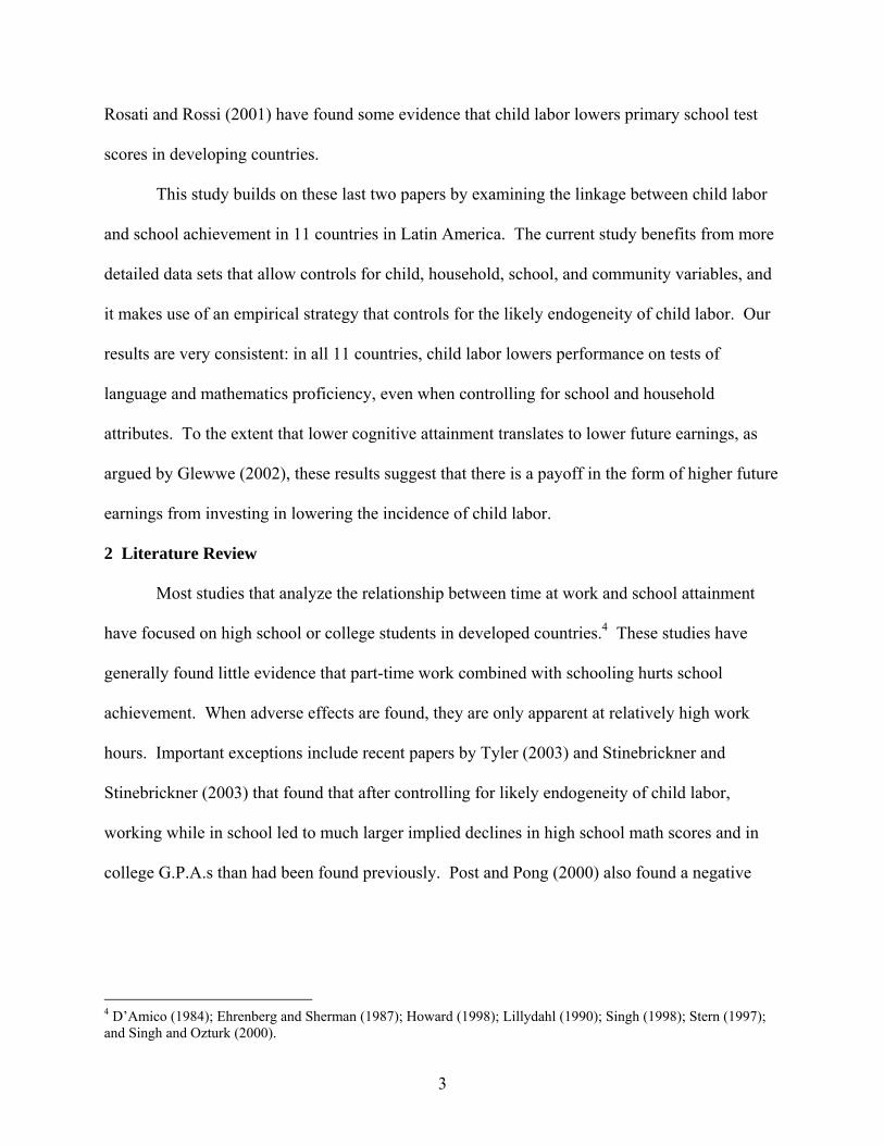
Rosati and Rossi (2001) have found some evidence that child labor lowers primary school test
scores in developing countries.
This study builds on these last two papers by examining the linkage between child labor
and school achievement in 11 countries in Latin America. The current study benefits from more
detailed data sets that allow controls for child, household, school, and community variables, and
it makes use of an empirical strategy that controls for the likely endogeneity of child labor. Our
results are very consistent: in all 11 countries, child labor lowers performance on tests of
language and mathematics proficiency, even when controlling for school and household
attributes. To the extent that lower cognitive attainment translates to lower future earnings, as
argued by Glewwe (2002), these results suggest that there is a payoff in the form of higher future
earnings from investing in lowering the incidence of child labor.
2 Literature Review
Most studies that analyze the relationship between time at work and school attainment
have focused on high school or college students in developed countries.4 These studies have
generally found little evidence that part-time work combined with schooling hurts school
achievement. When adverse effects are found, they are only apparent at relatively high work
hours. Important exceptions include recent papers by Tyler (2003) and Stinebrickner and
Stinebrickner (2003) that found that after controlling for likely endogeneity of child labor,
working while in school led to much larger implied declines in high school math scores and in
college G.P.A.s than had been found previously. Post and Pong (2000) also found a negative
4 D’Amico (1984); Ehrenberg and Sherman (1987); Howard (1998); Lillydahl (1990); Singh (1998); Stern (1997); and Singh and Ozturk (2000).

4
association between work and test scores in samples of 8th graders in many of the 23 countries
they studied.5
There are several reasons why the experience of older working students may not extend
to the experience of young children working in developing countries. Young children may be
less physically able to combine work with school, so that working children may be too tired to
learn efficiently in school or to study afterwards. Children who are tired are also more prone to
illness or injury that can retard academic development. It is possible that working at a young age
disrupts the attainment of basic skills more than it disrupts the acquisition of applied skills for
older students. School and work, which may be complementary activities once a student has
mastered literacy and numeracy, may not be compatible before those basic skills are mastered.
Past research on the consequences of child labor on schooling in developing countries has
concentrated on the impact of child labor on school enrollment or attendance. Here the evidence
is mixed. Patrinos and Psacharopoulos (1997) and Ravallion and Wodon (2000) found that child
labor and school enrollment were not mutually exclusive activities and could even be
complementary activities. However, Rosenzweig and Evenson (1977) and Levy (1985) found
evidence that stronger child labor markets lowered school enrollment. There is stronger evidence
that child labor lowers time spent in human capital production, even if it does not lower
enrollment per se. Psacharopoulos (1997) and Sedlacek et al. (2003) reported that child labor
lowered years of school completed and Akabayashi and Psacharopoulos (1999) discovered that
child labor lowered study time.
Nevertheless, school enrollment or attendance are not ideal measures of the potential
harm of child labor on learning because they are merely indicators of the time input into
5 This study included several developing countries including Colombia, Iran, South Africa, Thailand, and the Philippines which had the largest estimated negative effects of child labor on school achievement. However, the estimates do not control for school attributes or possible joint causality between school achievement and child labor.

5
schooling and not the learning outcomes. Even if child labor lowers time in school, it may not
hinder human capital production if children can use their limited time in school efficiently. This
is particularly true if the schools are of such poor quality that not much learning occurs in the
first place. On the other hand, the common finding that most working children are enrolled in
school may miss the adverse consequences of child labor on learning if child labor is not
complementary with the learning process at the lower grades. A more accurate assessment of the
impact of child labor on human capital production requires measures of learning outcomes, such
as test scores rather than time in school, to determine whether child labor limits or enhances
human capital production. Moreover, evidence suggests that cognitive skills, rather than years of
schooling, are the fundamental determinants of adult wages in developing countries (Glewwe,
1996; Moll, 1998). Therefore, identifying the impact of child labor on school achievement will
yield more direct implications for child labor’s longer term impacts on earnings and poverty
status later in the child’s life.
Direct evidence of child labor on primary school achievement is quite rare. Heady (2003)
found that child work had little effect on school attendance but had a substantial effect on
learning achievement in reading and mathematics in Ghana. Rosati and Rossi (2001) report that
in Pakistan and Nicaragua, rising hours of child labor is associated with poorer test scores. Both
of these studies have weaknesses related to data limitations. Heady treated child labor as
exogenous, but it is plausible that parents send their children to work in part because of poor
academic performance. Rosati and Rossi had no information on teacher or school characteristics,
although these are likely to be correlated with the strength of local child labor markets.
This study makes several important contributions to existing knowledge of the impact of
child labor on schooling outcomes in developing countries. First, it shows how child labor affects

6
test scores in 11 developing countries, greatly expanding the scope of existing research. Because
the same exam was given in all countries, we can illustrate how the effect of child labor on
cognitive achievement varies across countries that differ greatly in child labor incidence, per
capita income, and school quality. Because the countries also differ in the regulation and
enforcement of child labor laws, we can utilize cross-country variation in schooling ages and
truancy laws to provide plausible instruments for endogenous child labor. Finally, because the
data set includes a wealth of information on parent, family, community, school and teacher
attributes, we can estimate the impact of child labor on schooling outcomes, holding fixed other
inputs commonly assumed to explain variation in schooling outcomes across children. The
results are very consistent. Child labor lowers student achievement in every country. The
conclusions are robust to alternative estimation procedures and specifications. We conclude that
child labor has a significant opportunity cost in the form of foregone human capital production, a
cost that may not be apparent when only looking at enrollment rates for working children.
3 Theory and Economic Model
This section develops a tractable model of a household’s decision of whether to have a
child specialize in schooling or to split time between schooling and work. We assume the child
has only two uses of time, A: School attendance; and C: Child labor. Child time is normalized to
be one so that A + C = 1. The discussion is a simplified version of the model developed by
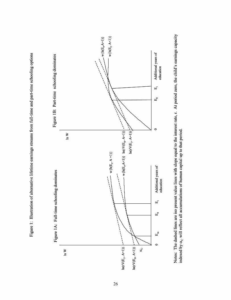
Rosen (1977). Figure 1A illustrates the tradeoff between entering the labor market at a young
age while attending school versus later entry with a longer period of specialization in schooling.6
6 Our discussion concentrates on pecuniary returns to schooling, as numerous studies have shown that child labor and time in school are sensitive to changes in pecuniary costs and returns. Nonpecuniary costs and returns are also likely to be important, but are more difficult to quantify. Most studies control for them using measures of household demographics and other proxies for local tastes toward schooling and child work, as we will in our empirical work.

7
The horizontal axis represents increasing levels of additional completed years of
schooling, Et. The vertical axis represents log earnings derived from human capital and local
labor demand, so that ,} Z,),H, A,,w{h(ElnW t εη= where h is a function that translates Et:
years of schooling; A: time intensity devoted to schooling; H: a vector of observable parent,
home, school and community variables; and a random error η ; into human capital production in
schools. The function w{} translates h, Z: a vector of local labor market factors; and ε : a
random error term; into the natural logarithm of earnings. Percent returns to schooling are
represented by the change in the height of w{}from a unit increase in Et. We assume that
schooling is subject to positive but diminishing returns so that wh > 0; hE > 0; and hEE < 0.7 We
also assume that the human capital produced per year spent in school is greater when
specializing in school (A = 1) than when sharing time between school and work (0 < A < 1).8
Children can gain earnings potential through on-the-job training as well as schooling, so
there is a possibility that early entry into the labor market will result in higher earnings than
would specializing in schooling for only a few years. This possibility is allowed by letting part-
time schooling result in higher wages at low levels of schooling. Eventually, the higher rate of
increase in human capital from schooling overtakes the initial gain to early labor market entry, so
at higher education levels, ).,),,1,w{h(E ) Z,H), , 1A ,{h(E tt εε ZHA <>=w
7 This allows for some increasing returns to schooling in the first few years of school. There is considerable evidence supporting the assumption of diminishing returns to schooling. Psacharopoulos (1994) presents the results of 57 studies of returns to schooling and average years of schooling in developing countries. A regression of estimated returns on years of schooling suggests that for each additional year of schooling, returns fall by 0.8 percentage points. Lam and Schoeni (1993) conducted a detailed examination of how rates of return to schooling changed as schooling increased in Brazil. After controlling for detailed family background variables, they found that the highest returns were to the first four years of schooling with nearly linear returns thereafter. Card’s (1999) review of the recent literature also concludes, albeit tentatively, that returns fall with years of education. It should be noted that finite life spans and rising opportunity costs of time as an individual ages guarantee that the returns to schooling must fall eventually. 8 Our formulation requires that when a child works (C>0), s/he must devote less time to schooling (A<1). This could mean the child attends school less frequently, or just that the child spends less time doing home work or reviewing.

8
Dropping H, Z and ε for ease of discussion, in figure 1A, maximizing lifetime income
would involve going to work immediately for all who plan to go to school Em additional years or
less and would involve full-time schooling for those planning to attend more than Em years. If a
child drops out at t = 0, s/he would have a lifetime wage equal to Cα .
The optimal choice of years of schooling involves setting the rate of growth of human
capital in school equal to the cost of borrowing. If r is the interest rate, this means choosing the
level of schooling, Et, such that r = tEw/∂∂ . The optimum is shown as the tangency between log
isopresent value lines that have a slope equal to r and the log wage function that has a slope
equal to tEw/∂∂ .9 As shown in figure 1A, generally there will be two levels of education that
satisfy that condition, E0 for the part-time schooling option and E1 for the full-time schooling
option. The parents should pick A = 1 or A < 1 depending on which yields the highest present
value. As drawn in figure 1A, the full-time schooling option (A = 1) dominates because
)1,V(E)1,V(E 01 <>= AA where ),V(Et A is the present value of the wage associated with a
given level of education, Et, and attendance choice, A.
However, full-time schooling will not always dominate part-time schooling. As r
increases, eventually the part-time schooling option will yield the higher present value, and at
even higher levels of r, the child will never go to school. Higher values of r would be expected
to be associated with lower household income to the extent that poorer households face more
constrained credit options, so children from poorer households will have lower enrollment rates
9 The log isopresent value lines have an intercept equal to the log of the present value of the wage weighted by the
interest rate. The continuous discounted present value formula is .}]),([{exp1),( trEer
WtrEAtEhw
rAtEV
−=−=
Taking logs and rearranging yields the familiar earnings function relationship, ,)ln(ln trErVW += where the logarithm of the wage is linear in years of schooling. The fuller specification would include elements of H, Z, and ε as well.

9
and higher incidence of working while in school than will children from better off families.10
One rationale for government intervention in the child labor market is that if the government’s
discount rate is less than that of credit constrained households, the household will select a lower
level of schooling than the government would prefer.
In general, factors that flatten the profile for w{h(Et, A = 1)}, such as poor school quality
or poor parental support for schooling, will increase the likelihood that the child will work while
in school, if not forego schooling altogether. Figure 1B illustrates this point. Holding r at the
same level as in 1A, the flatter profile for w{h(Et, A = 1)} results in the part-time schooling
option, E0, having the higher present value of earnings relative to the full time option, E1.
Similarly, factors that make the profile for w{h(Et, A < 1)} steeper, such as having relatively
higher local wages for child laborers or relatively lax local enforcement of child labor laws, will
raise the present value of the part-time option versus full-time schooling option.
Given the formulation in figure 1 and reintroducing H , Z, and ε , a household will send a
child to work when ),,,1,V(E),,,1,V(E 01 εε ZHAZHA <<= . This condition implies a
reduced form child labor supply equation that is a function of the exogenous factors that steepen
or flatten the two earnings profiles, w{h(Et, A = 1, H , Z, ε )} and w{h(Et, A < 1, H , Z, ε )};
i.e.
(1) C = g(H, Z, ε )
Equation (1) is critical for the purpose of estimating the impact of child labor on human capital
production in schools. Letting Q be an observable measure of cognitive skills produced in
school, the human capital production process generating earnings will be of the form
(2) Q = h(Et, A, H, η ) = q(Et, C, H, η )
10 Evidence consistent with these predictions can be found in Sedlacek et al. (2003).

10
In the empirical application to follow, the level of education, Et, is set at grades 3-4 for all
children in the sample. However, child labor C is endogenous and is selected jointly with
information on the child’s progress in school, as measured by Q. Consequently, Var( ε , 0) ≠η ,
and ordinary least squares estimation of (2) will be biased. Equation (1) suggests that elements
of the vector Z that shift w{} can be used to identify C in equation (2), where Z includes
variables that alter the child’s value of time in the local labor market but do not directly affect
school achievement.
A. Factors Shifting the Probability of Child Labor
Because our data set includes several different countries, there is considerable variation
in the laws regulating child labor. Mandatory school starting ages range from 5 to 7, the earliest
allowable school leaving age varies from 12 to 16, and some countries require attendance at
preschool. Countries may vary in their ability to enforce these laws. If parents do not fear being
caught having their children work, or do not fear sanctions or fines if caught, the expected
returns to child labor rises relative to the returns to schooling. Countries also differ in their
acceptance of early marriage, an alternative use of time to schooling. While our children are too
young to marry, the potential of early marriage may shift the expected returns to time out of
school versus time in school.
These differences in laws and cultures regulating child labor alter the age at which
children would normally enter grades 3 and 4, and thus alter the opportunity costs of being in
grades 3 and 4 differ across countries. We do not have information on local wages, although as
most child labor is unpaid work for family enterprises, information on wages would not
adequately capture the value of time outside school. Instead, we utilize the presumed upward
relationship between the marginal productivity of child labor and the child’s age which we

11
assume is driven largely by physical stature.11 Interactions between measures of a country’s
legal or cultural restrictions on child labor and child age and its square are used to capture
exogenous variation in the height and slope of w{h(Et, A = 1, H , Z, ε )} versus w{h(Et, A < 1,
H , Z, ε )}. These shifts in the net return to time in school provide the needed exogenous shift in
C.12 Within countries, interactions between age, gender and urban versus rural residence
captures variation in the net return to being in school between boys and girls and between urban
and rural markets. We illustrate the impact of this identification strategy in figures 2 and 3
discussed below.
B. Factors Affecting School Outcomes
Estimation of equation (2) follows the educational production function literature in that Q
is measured by test scores that are explained by variables characterizing the student’s parents,
household, teacher, school and community (Hanushek, 1985). Measures used include most of
those that have been found to be important in developing country settings (Hanushek, 1995;
Kremer, 1995).
Estimates of educational production functions are subject to numerous biases.13 Among
the most commonly discussed is the lack of adequate control for the student's innate ability.14
Many studies have attempted to correct for the problem by using two test scores taken at
different times. If ability has an additive effect on school achievement, the difference between
11 Rosenzweig (1980) found that wages for day labor in India were primarily driven by stature and not by acquired education. 12 Angrist and Krueger (1991) use variation in compulsory school starting ages across states to instrument for endogenous time in school in their analysis of returns to schooling using U.S. Census data. Tyler (2003) uses variation in state child labor laws to instrument for child labor in his study of U.S. high school tests scores. We began with a large number of interactions, but the resulting variables were highly collinear, and so we used a parsimonious subset of the fuller specification. 13 See Glewwe (2002) for a comprehensive review of the problems associated with estimating educational production functions. 14 Ability bias has also been the subject of numerous papers estimating returns to schooling. The consensus is that the bias is small (Card, 1999). If earnings and cognitive skills are closely tied, as argued by Glewwe (2002), then the role of ability bias should be small in educational production estimates also.

12
the two output measures will be purged of the ability effect. The data for the current study only
includes tests taken at one point in time, so the differencing option is not available. However,
there are reasons why undifferenced data may yield satisfactory or even preferred estimates to
the differenced data. As Glewwe (2002) argues, if measures of H vary slowly over time, the
value of the differenced measure of achievement is minimal. This is more likely to be true at the
earliest stages of schooling where there is less variation in curriculum, educational materials or
teacher training. Furthermore, the use of parental attributes such as education and income should
partially control for inherited ability. Finally, if there is considerable measurement error in
estimates of Q, the level of Q may be measured more reliably than the change in Q. In any
event, the results of the production function estimation in this study should be interpreted as
cumulative as of grade 3 or 4 rather than the additional learning obtained in that grade.
4 Data
In 1997, the Latin-American Laboratory of Quality of Education (LLECE) carried out the
First Comparative International Study on Language, Mathematics and Associated Factors for 3rd
and 4th graders in Latin America. LLECE collected data initially in 13 countries, but the required
information was only available for 11: Argentina, Bolivia, Brazil, Chile, Colombia, Honduras,
Mexico, Paraguay, Peru, Dominican Republic and Venezuela15.
The data set is composed of a stratified sample designed to insure sufficient observations
of public, private, rural, urban and metropolitan students in each country. Data were collected on
40 children from each of 100 schools in each country for a total of 4,000 observations per
country. Half of the students were in the 3rd grade and half in the 4th grade. For budgetary
reasons, LLECE had to use a priori geographic exclusions to limit the transportation and time
15 Costa Rica was included in the initial data collection but LLECE dropped their data due to consistency problems. Cuba was excluded due to missing data on child labor.

13
costs of data collection. Very small schools with too few 3rd and 4th graders and schools in
remote, difficult to access, or sparsely inhabited regions were excluded. Because of the cost of
translating exams, schools with bilingual or indigenous language instruction were also
excluded.16
Survey instruments consisted of tests administered to the sample of children of the
sampled schools, and self-applied questionnaires to school principals (Pr), to the teachers (T) and
parents (or legal guardians) (P) of the tested children, and to the children themselves (C). In
addition, surveyors collected information on the socioeconomic characteristics of the community
(S). A description of the variables used in the Latin America analysis can be found in Table 1.
Summary statistics are reported in Table 2.17
All children were tested in mathematics, and all were tested in Spanish except the
Brazilian children who were tested in Portuguese. It should be noted that the tests and
questionnaires were given only to children who attend school, so no information was obtained on
children who are not in school. Therefore the results can only be applied to enrolled children.
However, the great majority of working children in the age ranges typical of 3rd and 4th graders
in Latin America are enrolled in school, so the bias is likely to be modest.
Child labor is measured by each child’s response to a question asking whether s/he is
engaged in work outside the home. Children could choose from three alternatives describing
their work: s/he “almost never”, “sometime” or “often” works outside the home. The
concentration on paid work outside the home avoids some definitional problems related to
16 For a detailed description of the a priori exclusions in each country, consult Table III.6 of the Technical Bulletin of the LLECE. 17 For some reason, language scores were reported for three percent more students than were mathematics scores. The missing mathematics scores appeared to be due to random reporting errors as there were no large differences between the sample means of the group taking the mathematics and language tests. We report the means from the sample taking the language exam.
14
distinguishing between unpaid work for the home enterprise and household chores. Furthermore,
the debate over the harmful effects of child labor generally does not include working in the
home. Nevertheless, this measure may understate the actual incidence of child labor, particularly
for girls who are more likely than boys to be engaged in housework.
The countries differed in legal regulations and social norms governing child labor. We
add measures of these factors from other sources as external factors affecting the probability of
child labor across countries. Information on compulsory schooling laws for each country was
obtained from the UNESCO (2002). While countries may legislate child labor, the laws may not
be effectively enforced. Kaufmann, Kraay and Zoida-Lobatón (2002) develop various measures
of the legal environment for each of the countries in our sample. We use their measure of each
country’s ability to enforce its laws as an indicator of the likelihood that child labor laws are
effective. The percentage of women aged 15 to 19 that are married was used as an indicator of
cultural acceptance of early marriage (United Nations Statistics Division, 2000).
The role of physical stature in child labor creates a highly nonlinear pattern in the
probability of child labor with respect to age. Under age ten, there is almost no discernible
relationship between age and the incidence of child labor, but the relationship is strong and
positive thereafter. To capture this, we create a spline in age that is used in the child labor
equation. A dummy variable, d10, takes the value of one for children under 10 and zero
otherwise. For children aged 10 and over, the effect of age is captured by interactions between
(1-d10) and age. Thus, the age effect on child labor is held constant until age 10.
Most of the other exogenous variables are self-explanatory. However, the measure of the
classroom environment, inadequacy, requires some explanation. Teachers were asked the extent
to which they judged classroom lighting, classroom temperature, classroom hygiene, classroom

15
security, classroom acoustics, language textbooks, mathematics textbooks and all textbooks to be
inadequate. The weighted sum of the responses is used as the aggregate index of school
shortages, where the weights were taken as the first principal component from a factor analysis
of the teachers’ responses.
A preliminary assessment of the interrelationship of child labor and schooling can be
seen in Table 3. Unconditional means of the mathematics and language test scores are reported
by self-reported intensity of child labor in columns two and four. Across 11 countries and two
achievement tests, 22 cases in all, the pattern never varies. Children who work only some of the
time outperform those who often work. Children who almost never work outperform those who
work sometimes or often. The differences are almost always statistically significant. The
advantage is large for children who almost never work over those who often work, averaging
25.0 percent on the mathematics exam and 29.5 percent on the language exam. The advantage
over occasional child laborers is much smaller, averaging 8.1 percent in mathematics and 8.8
percent in languages.
Variation in child labor could be correlated with variation in the child, household,
teacher, school and community variables defined in Table 1. In particular, the incidence of child
labor would be expected to be higher in communities with weaker schools and lower parental
inputs, and so the absence of these variables would be expected to bias the coefficient on child
lab or downward. Consistent with that presumption, adding controls for parental and school
inputs decreases the magnitude of the adverse effects of child labor on test scores. Nevertheless,
across all countries and both tests, child labor still significantly reduces school achievement,
holding parental and school inputs fixed. Children who never work score between 15-19 percent
higher than children who often work. Occasional child workers score 6-7 percent higher than

16
children who often work. The large gap between children who almost never work and those who
work occasionally or frequently suggests that there is a significant opportunity cost in the form
of lost cognitive skills when young children work while enrolled in school.
5 Econometric Strategy
The results in Table 3 suggest a strong negative effect of child labor on school
achievement, but the effect may be in the reverse direction– poor schooling outcomes leading to
child labor. The direction of this bias is difficult to predict. The most plausible is that poor
school performers are sent to work so that the OLS coefficient on child labor will be biased
downward. However, Both Tyler (2003) and Stinebrickner and Stinebrickner (2003) found
biases in the opposite direction for older students, so the better students were more likely to
work. Measurement error in the self-reported incidence of child labor could also bias the
estimated coefficient of child labor on schooling outcomes. The cumulative direction of these
sources of bias cannot be established, but both simultaneity and measurement error can be
handled by the use of plausible instruments that alter the probability of engaging in child labor
without directly affecting test scores.
The first step in the estimation process is to predict child labor. Our categorical measure
of child labor includes 0 (almost never work); 1 (sometime work); and 2 (often work). An
ordered probit specification of equation (1) was attempted first, but the model could not
distinguish children who occasionally worked from children who worked often. Therefore, we
reverted to a simple probit model predicting the incidence of child labor as a function of child,
parent school, community and legal variables. Predicted child labor from (1) is used as the
measure of C in estimating equation (2). This two-stage estimation leads to consistent, but
inefficient estimates of the parameters of the achievement equation. We utilize a bootstrapping

17
method in which 100 samples with replacement are drawn from the original data, subjected to
the ordered probit estimation and then inserted into the second stage achievement equation in
order to simulate the sampling variation in the estimates. The bootstrap standard errors are
reported for all estimates.
6 Empirical Results
A. Equations Explaining Child Labor
Estimates from the probit child labor supply equation are reported in Table 4.
Observations for Venezuela had to be dropped because child age was not reported. Mexico’s
mathematics results also had to be dropped because missing child identifiers prevented us from
merging in age information from the language sample. Because the two samples are not
identical, we report separate estimates for the samples of children taking the mathematics and
language exams. The coefficient estimates in the two samples do not differ in either sign,
magnitude, or significance.
Boys are more likely than girls to work outside the home, and rural boys and girls work
more than their urban counterparts. Children of more educated parents and who have access to
more books in the home are less likely to work, as are children who received some preschool
education. School quality also affects the incidence of child labor. Schools with inadequate
supplies or learning environment encourage child labor. Children who have male teachers and
more non-Spanish or non-Portuguese language speakers among their peers are also more likely
to work outside the home. In general, these results suggest that better schooling inputs in the
home or at school lower the incidence of child labor. That exception is that children are more
likely to work if their school has more educated teachers.

18
Variation in the legal and cultural environment regulating child labor appears to matter.
The joint test of the null hypothesis that the instrumental variables have no effect on child labor
is easily rejected. More stringent truancy regulations lower the incidence of child labor in that
older school leaving ages lower the child labor participation rate. The effect is greater if the
country has a reputation for enforcing its laws. Early marriage works in the opposite direction.
Because of the large number of interaction terms, it is useful to simulate how the various
factors shift the labor supply profiles as the child ages. Figure 2 illustrates how regional
variation in the market for child labor shifts child labor supply for boys and girls. The dummy
variable spline effectively fixes child labor intensity for children under ten. After age ten, child
labor intensity rises for both boys and girls. The slight dip in labor supply at age 10 is a
consequence of the quadratic specification after age 10, but that specification proved the best
fit.18 In each market, boys work more than girls.19 The higher market labor force participation
for boys is consistent with the presumption that the marginal product of child labor is higher for
boys than girls. However, rural girls have higher labor force participation than metropolitain
boys.
Figure 3 illustrates how laws changing the minimum school leaving age alter the labor
supply profiles. Younger school leaving ages raise the child labor supply at the youngest ages,
but the profiles rise more rapidly after age 10 in countries with the older school leaving ages. In
this way, the legal environment regulating child labvor changes both the height and the slope of
the child labor force participation profiles.
B. The Impact of Continuous Measures of Child Labor on Achievement
18 The second stage estimates were not sensitive to changing the end age of the spline to 8 or 10 or to other alternative specifications of the age-supply profile. 19 We truncate ages below eight (0.4% of the sample) and above 15 (0.8% of the sample) as we do not have sufficient observations at the lower and higher ages to generate reliable child labor supply trajectories.

19
Table 5 reports the results from estimating equation (2) both with and without controls
for the endogeneity of child labor. In the specification in Table 5, when child labor is treated as
exogenous, it takes the values of 0 (seldom working); 1 (sometime working); or 2 (frequently
working). When treated as endogenous, child labor is a continuous variable with domain over
the real line taken as the fitted values from the ordered probit estimation in Table 4. The rest of
the regressors are the child, household, parent and school variables used as regressors in Table
4.20
The impact of child labor on test scores is negative and significant whether or not child
labor is treated as exogenous or endogenous. 21 Because of the difference in the scale of the
measured child labor across the two specifications, it is difficult to directly compare the
magnitude of the implied effect of child labor on test scores. The implied percentage effect of
moving from level 0 to level 1 (seldom working to sometime working) is -0.8 percent for both
the mathematics and language exams. In contrast, the estimated impact of a ten percent increase
in the child labor index derived from the ordered probit equation is a 1.6 percent decrease in the
mathematics exam and a 2.1% decrease in the language exam. A better sense of the comparison
between the two estimates can be found in Figures 4-5 which traces out the predicted
mathematics and language test scores at each decile of the reported and predicted child labor
distributions. At the break points of the exogenous measure (ie going from child labor level 0 to
level 1 at the 44th percentile and from level 1 to level 2 at the 77th percentile) the predicted test
scores are nearly identical between the two measures. However, the relationship is steeper at the
upper and lower tails of the distribution of predicted child labor. The implication is that by
20 We obtained similar estimates of the adverse effect of child labor on test scores when we used a school-specific fixed effect to control for the impact of variation in school and community variables instead of the vector of school and community variables. 21 The Davidson-MacKinnon (1993, pp. 237-240) variant of the Hausman test easily rejected the assumption of exogeneity of child labor.

20
restricting the range of child labor to three discrete levels, the impact of child labor on test scores
in the first two columns of Table 5 is understated.
Most of the other variables have similar effects across the two sets of estimates in Table
5. There are two main exceptions. The adverse effects of being a boy or being in a rural school
disappear in the instrumented equations. Gender and rural residence are closely tied to the
incidence of child labor. It is likely that the negative effects of being male and being in a rural
area on test scores is related to the indirect effect of these variables on the higher probability that
male and rural children work.
C. The Impact of Discrete Measures of Child Labor on Achievement
The difference in the magnitudes of the child labor effects reported in Table 5 correspond
to two issues, measurement error related to the use of discrete versus continuous measures of
child labor and the problem of endogeneity. Table 6 attempts to explore the role of endogeneity
in isolation by converting the predicted index value from the ordered probit back into a discrete
measure so that the scale of measurement is the same across the two sets of estimates. In
practice, the model could not clearly distinguish between children predicted to work sometime
versus often. Only one percent of the children were predicted to work often, so we combined the
two measures into one. We also reconverted the exogenous child labor indicator into a
dichotomous variable distinguishing “working seldom” (0) from “working sometime or often”
(1).22
When self-reported child labor is treated as exogenous, math scores fall by 12.4 percent
and language scores fall by 13.4 percent for children who work sometime or often compared to
those who seldom work. Unlike the findings reported by Tyler (2003) and Stinebrickner and
22 Virtually identical results are obtained when we use a probit to estimate the transformed dichotomous labor supply equation rather than the ordered probit equation in Table 4. The results in Table 6 use predictions based on the ordered probit estimates.

21
Stinebrickner (2003) for older U.S. students, treating child labor status as endogenous lowers
these estimates: mathematics scores fall by 7.5 percent and language scores fall by 7 percent.23
Our results are consistent with the hypothesis that parents are more likely to send their children
to work outside the home when the child is not doing well in school, so that part of the estimated
negative effect of child labor on primary school test scores is attributable to this reverse
causality. Nevertheless, the finding that child labor significantly lowers test scores still holds
after controlling for endogeneity.
Glewwe’s (2002) review of the human capital literature in developing countries argued
that cognitive ability as measured by test scores is strongly tied to later earnings as an adult. We
would therefore expect that returns to schooling for those who worked as children should be
lower than for those who did not work, all else equal. Consistent with that expectation, Ilahi et
al. (2003) found that, holding constant years of schooling completed, Brazilian adults who
worked as children received 4 to 11 percent lower returns per year of schooling. Therefore, our
findings regarding the adverse effects of child labor on test scores correspond closely in
magnitude to findings elsewhere of adverse impacts of child labor on earnings.
7 Conclusions
Working outside the home lowers average school achievement in samples of 3rd and 4th
graders in each of the 11 Latin American countries studied. Child labor is shown to have
significant adverse effects on mathematics and language test scores using various specifications
correcting for possible endogeneity and measurement error in self-reported child labor intensity. 23 In unreported least-squares regressions, children working some of the time experienced a 10 percent reduction in mathematics scores and an 11 percent reduction on the language exam. The associated decline in test score for children who report working often were 16 percent and 17 percent respectively. Two-stage estimates that relied on several more instruments that measured variation in school starting age and mandatory preschool across countries were able to distinguish between “sometime” versus “often” working. The parameters on the instrumented child labor were almost identical to the least squares estimates in magnitude and significance. Because several of these additional instruments had only weak correlation with test scores in reduced-form equations, we preferred the more parsimonious representation discussed in the text.

22
Children who work even occasionally score an average of 7 percent lower on language exams
and 7.5 percent lower on mathematics exams. There is some evidence that working more
intensely lowers achievement more, but these results are more speculative in that empirical
models were unable to distinguish clearly between working “sometime” versus working “often”.
These adverse effects of child labor on cognitive ability are consistent in magnitude with
estimated adverse effects of child labor on earnings as an adult. Thus, it is plausible that child
labor serves as a mechanism for intergenerational transmission of poverty, consistent with
empirical evidence presented by Emerson and Souza (2003) and the theoretical models of
poverty traps advanced by Basu (2000), Basu and Van (1998), and Baland and Robinson (2000).
Such large effects suggest that efforts to combat child labor may have substantial payoffs
in the form of increased future earnings or lower poverty rates once children become adults.
How to combat child labor is less clear. Our child labor supply equations suggest that truancy
laws appear to have some effect in lowering the incidence of child labor. However, most of the
variation in child labor occurs within countries and not across countries, so policies must address
local child labor market and poverty conditions as well as national circumstances in combating
child labor. Policies that alter the attractiveness of child labor or bolster household income, such
as income transfer programs that condition receipt on child enrollment or reduced child labor, are
likely candidates. Recent experience on such programs in Brazil, Honduras, Mexico and
Nicaragua would appear to support further development and expansion of such conditional
transfer programs.

23
References
Akabayashi, Hideo and George Psacharopoulos. 1999. “The Trade-off between Child Labor and Human Capital Formation: A Tanzanian Case Study.” Journal of Development Studies 35 (June): 120-40. Angrist, Joshua D. and Alan B. Krueger. 1991 “Does Compulsory School Attendance Affect Schooling and Earnings? Quarterly Journal of Economics 106 (November): 979-1014. Baland, Jean-Marie and James A. Robinson. 2000. “Is Child Labor Inefficient?” Journal of Political Economy 108 (August):663-679. Basu, Kaushik. 2000. Analytical Development Economics: The Less Developed Economy Revisited. Cambridge, MA: The MIT Press. Basu, Kaushik and Pham Honang Van. 1998. “The Economics of Child Labor.” American Economic Review 88 (June): 412-427. Card, David. 1999. “The Causal Effect of Education on Earnings.” In Ashenfelter and Card, eds. Handbook of Labor Economics Vol. 3A. Amsterdam: Elsevier Science B.V. . D’Amico, Ronald. 1984. ”Does Employment During High School Impair Academic Progress?” Sociology of Education 3 (July):152-164. Davidson, Russell and James G. MacKinnon. 1993. Estimation and Inference in Econometrics Oxford: Oxford University Press. Ehrenberg, Ronald G. and Daniel R, Sherman. 1987. ”Employment While in College, Academic Achievement, and Postcollege Outcomes.” The Journal of Human Resources 22 (Winter):1-23. Glewwe, Paul. 1996. “The Relevance of Standard Estimates of Rates of Return to Schooling for Educational Policy: A Critical Assessment.” Journal of Development Economics 51 (2):267-290. Glewwe, Paul. 2002. “Schools and Skills in Developing Countries: Educational Policies and Socioeconomic Outcomes.” Journal of Economic Literature 50 (June):436-482. Hanushek, Eric A. 1995. “Interpreting Recent Research on Schooling in Developing Countries.” The World Bank Research Observer 10 (August):227-246. Heady, Christopher. 2003. “What is the Effect of Child Labour on Learning Achievement? Evidence from Ghana.” World Development. Howard, Ian. 1998. ”Does Part-Time Employment Affect A-level Grades Achieved?” PSSI Forum N26 (October):10-11.

24
Ilahi, Nadeem, Peter F. Orazem and Guilherme Sedlacek. 2003. “How Does Working as a Child Affect Wages, Income and Poverty as an Adult?” in Peter F. Orazem and Guilherme Sedlacek eds. Eradicating Child Labor in Latin America in the 90s: The Promise of Demand Side Interventions. Forthcoming. Kaufmann, Daniel, Aart Kraay and Pablo Zoida-Lobatón. 2002. “Governance Matters II: Update Indicators for 2000/01.” World Bank Policy Research Working Paper #2772 (February). Kremer, Michael R. 1995. Research on Schooling: What We Know and What We Don't: A Comment on Hanushek. The World Bank Research Observer 10 (August): 247-254. Lam, David and Robert F. Schoeni. 1993. “Effects of Family Background on Earnings and Returns to Schooling: Evidence from Brazil.” Journal of Political Economy 101 (August):710-740. Levy, Victor. 1985. “Cropping Pattern, Mechanization, Child Labor, and Fertility Behavior in a Farming Economy: Rural Egypt.” Economic Development and Cultural Change 33 (July):777-791. Lillydahl, Jane H. 1990. ”Academic Achievement and Part-Time Employment of High School Students.” Journal of Economic Education 21 (Summer):307-316. Moll, Peter. 1998. “Primary Schooling, Cognitive Skills and Wages in South Africa.” Economica 65:263-284. Patrinos, Harry A. and George Psacharopoulos. 1997. “Family Size, Schooling and Child Labor in Peru - An Empirical Analysis.” Journal of Population Economics 10 (October): 387-405. Post, David and Suet-ling Pong. 2000. “Employment During Middle School: The Effects on Academic Achievement in the U.S. and Abroad.” Educational Evaluation and Policy Analysis 22 (Fall): 273-298. Psacharopoulos, George. 1994. “Returns to Investment in Education: A Global Update.” World Development 22:1325-1343. Psacharopoulos, George. 1997. “Child Labor versus Educational Attainment: Some Evidence from Latin America.” Journal of Population Economics 10:337-386. Ravallion, Martin and QuentinWodon. 2000. “Does Child Labor Displace Schooling? Evidence on Behavioral Responses to an Enrollment Subsidy.” Economic Journal. Forthcoming. Rosati, Furio Camillo and Mariacristina Rossi. 2001. “Children’s Working Hours, School Enrolment and Human Capital Accumulation: Evidence Form Pakistan and Nicaragua.” Understanding Children’s Work. UNICEF Innocenti Research Centre.

25
Rosen, Sherwin. “Human Capital: A Survey of Empirical Research.” in R. Ehrenberg ed. Research in Labor Economics Vol. 1. Amsterdam: JAI Press. 1977.
Rosenzweig, Mark R. 1980. “Neoclassical Theory and the Optimizing Peasant: An Econometric Analysis of Market Family Labor Supply in a Developing Country.” Quarterly Journal of Economics 94 (February):31-55. Rosenzweig, Mark R. and Robert Evenson. 1977. “Fertility, Schooling and the Economic Contribution of Children in Rural India: An Econometric Analysis.” Econometrica 45 (July): 1065-79. Sánchez, Mario A., Peter F. Orazem and Victoria Gunnarsson. 2003. “The Effect of Child Labor on Mathematics and Language Achievement in Latin America.” in Peter F. Orazem and Guilherme Sedlacek eds. Eradicating Child Labor in Latin America in the 90s: The Promise of Demand Side Interventions. Forthcoming. Sedlacek, Guilherme, Susanne Duryea, Nadeem Ilahi and Masaru Sasaki. 2003. “Child Labor, Schooling, and Poverty in Latin America.” in Peter F. Orazem and Guilherme Sedlacek eds. Eradicating Child Labor in Latin America in the 90s: The Promise of Demand Side Interventions. Forthcoming. Singh, Kusum. 1998. ”Part-Time Employment in High School and its Effect on Academic Achievement.” The Journal of Educational Research 91 (January/February):131-139. Singh, Kusum and Mehmet Ozturk. 2000. “Effect of Part-time Work on High School Mathematics and Science Course Taking.” Journal of Educational Research, 91(2):67–74. Stern, David. 1997. “Learning and Earning: The Value of Working for Urban Students.” ERIC Digest #128. Stinebrickner, Ralph and Todd R. Stinebrickner. “Working During School and Academic Performance.” Journal of Labor Economics 21 (April 2003): 473-491. Tyler, John H. “Using State Child Labor Laws to Identify the Effect of School-to-Work on High School Achievement.” Journal of Labor Economics 21 (April 2003): 381-408. UNESCO. 2002. Education Statistics 2001-Regional Report on Latin America. (http://portal.unesco.org/uis). November, 2002.
United Nations Statistics Division. 2000. The World’s Women 2000: Trends and Statistics. (http://unstats.un.org/unsd/demographic/ww2000/table2a.htm). January, 2003.
26
w{h
(Et,A
=1)}
w{h
(Et,
A<1
)}w
{h(E
t, A
=1)
}
w{h
(Et,A
<1)}
lnW
lnW
ln(r
V(E
0, A
=1))
ln(r
V(E
1, A
=1))
ln(r
V(E
1, A
=1))
ln(r
V(E
0, A
<1))
0
E
mE 0
E 1A
dditi
onal
yea
rs o
fed
ucat
ion
0E 0
E 1A
dditi
onal
yea
rs o
fed
ucat
ion
αC
Figu
re 1
: Ill
ustra
tion
of a
ltern
ativ
e lif
etim
e ea
rnin
gs st
ream
sfro
m fu
ll-tim
e an
d pa
rt-tim
e sc
hool
ing
optio
ns
Figu
re 1
A:
Full-
time
scho
olin
g do
min
ates
Figu
re 1
B:
Part-
time
scho
olin
g do
min
ates
Not
es:
The
dash
ed li
nes a
re is
opr
esen
t val
ue li
nes w
ith sl
ope
equa
l to
the
inte
rest
rate
, r.
At p
erio
d ze
ro, t
he c
hild
’s e
arni
ngs c
apac
ity
inde
xed
by α
Cw
ill re
flect
all
accu
mul
atio
ns o
f hum
an c
apita
l up
to th
at p
erio
d.
w{h
(Et,A
=1)}
w{h
(Et,
A<1
)}w
{h(E
t, A
=1)
}
w{h
(Et,A
<1)}
lnW
lnW
ln(r
V(E
0, A
=1))
ln(r
V(E
1, A
=1))
ln(r
V(E
1, A
=1))
ln(r
V(E
0, A
<1))
0
E
mE 0
E 1A
dditi
onal
yea
rs o
fed
ucat
ion
0E 0
E 1A
dditi
onal
yea
rs o
fed
ucat
ion
αC
Figu
re 1
: Ill
ustra
tion
of a
ltern
ativ
e lif
etim
e ea
rnin
gs st
ream
sfro
m fu
ll-tim
e an
d pa
rt-tim
e sc
hool
ing
optio
ns
Figu
re 1
A:
Full-
time
scho
olin
g do
min
ates
Figu
re 1
B:
Part-
time
scho
olin
g do
min
ates
Not
es:
The
dash
ed li
nes a
re is
opr
esen
t val
ue li
nes w
ith sl
ope
equa
l to
the
inte
rest
rate
, r.
At p
erio
d ze
ro, t
he c
hild
’s e
arni
ngs c
apac
ity
inde
xed
by α
Cw
ill re
flect
all
accu
mul
atio
ns o
f hum
an c
apita
l up
to th
at p
erio
d.

27
Figure 2: Child Labor Participation Profiles by Age, Gender and Location (based on estimates from Table 4)
0.7
0.75
0.8
0.85
0.9
0.95
1
1.05
1.1
8 9 10 11 12 13 14
Age
Nor
mal
ized
Inde
x Va
lue
of C
hild
Lab
or Rural Boys
Rural Girls
Metropolitan Boys
Metropolitan Girls
Figure 3: Child Labor Participation by Age and Oldest Age of Compulsory Schooling
(based on estimates from Table 4)
0.8
0.85
0.9
0.95
1
1.05
1.1
1.15
1.2
8 9 10 11 12 13 14
Age
Nor
mal
ized
Inde
x Va
lue
of C
hild
Lab
or
Truancy Age 14
Truancy Age 12

28
Figure 4: Predicted Mathematics Test Scores by Child Labor Decile, based on estimates from Table 5
(Maximum Score = 32, Average = 15.4)
8
10
12
14
16
18
20
0 10 20 30 40 50 60 70 80 90 100
Child Labor Decile
Pred
icte
d M
athe
mat
ics
Test
Sco
res Ordered Probit Estimate,
Child Labor Endogenous
OLS Estimate, Child Labor Exogenous
Figure 5: Predicted Language Test Scores by Child Labor Decile, based on estimates from Table 5
(Maximum Score = 19, Average = 11.8)
8
9
10
11
12
13
14
15
0 10 20 30 40 50 60 70 80 90 100
Child Labor Decile
Pred
icte
d La
ngau
ge T
est S
core
s
Ordered Probit Estimate, Child Labor Endogenous
OLS Estimate, Child Labor Exogenous

29
Table 1: Variable Description Endogenous variables Math Score Mathematics test score (C) Language Score Language test score (C) Work Outside Index of how often student works outside the home (0-2) (C) Often Student reports that s/he often works outside the home (C) Sometime Student reports that s/he sometimes works outside the home (C) Almost Never Student reports that s/he almost never works outside the home (C)
Exogenous variables Child Age Student age (years) (C) d10 Dummy if student is below 10 years old Boy Dummy if student is a boy (C) No Preschool Student did not attend preschool/kindergarten (C) Parents/Household Parent Educ Average education of parent(s) or guardian(s) (P) Books at Home Number of books in student’s home (P) Teacher Male Dummy if teacher is male (T) Teacher Educ Aggregated teacher education (T) School Spanish Enr Total number of Spanish (Portuguese) speaking students enrolled (Pr) Inadequacy Index of school supply inadequacy (Pr) Math/week Number of mathematics classes per week (Pr) Spanish/week Number of Spanish (Portuguese) classes per week (Pr) Community (Reference: Metropolitan area with 1M people or more) Urban Dummy variable indicating if school is located in an urban area (2,500-1M people) (S) Rural Dummy variable indicating if school is located in a rural area (less than 2,500 people) (S) Instruments Legal structure Comp End Age Compulsory school ending age in the country (U) Preprimary Dummy variable indicating if the country has a compulsory preprimary school year (U) Marriage Percentage of 15-19 year olds married in the country (UN) Law Estimate of the degree of rule of law 2000/01 (KKL) Sources: C: Child survey or test; P: Parent’s survey; T: Teacher’s survey; Pr: Principle’s survey; S: Survey Designer’s observation; U: UNESCO estimate (2002); UN: UN (2000); KKL: Estimate taken from Kaufmann, Kraay and Zoida-Lobatón (2002).

30
Table 2: Summary Statistics Variable N Mean Std. Dev. Min Max Endogenous variables Mathematics Score 28939 15.38 6.17 0 32 Language Score 34306 11.81 4.37 0 19 Work Outside 34306 0.78 0.79 0 2 Often 34306 0.23 0.42 0 1 Sometime 34306 0.33 0.47 0 1 Almost Never 34306 0.44 0.50 0 1 Exogenous variables Child Age 34306 9.71 1.45 6 18 d10 34306 0.79 0.41 0 1 Boy 34306 0.50 0.50 0 1 No Preschool 34306 0.24 0.42 0 1 Parents/Household Parent Educ 34306 2.75 1.62 0 6 Books at Home 34306 2.40 0.90 1 4 Teacher Male 34306 0.21 0.41 0 1 Teacher Educ 34306 1.45 0.54 0 2 School Spanish Enr 34306 519.15 553.69 0 6026 Inadequacy 34306 0.43 1.11 -0.83 3.33 Spanish/week 34306 6.16 3.34 0 30 Community Urban 34306 0.47 0.50 0 1 Rural 34306 0.29 0.45 0 1 Instruments Legal structure Comp End Age 34306 13.72 1.01 12 16 Marriage 34306 16.14 4.88 12 29 Law 34306 -0.24 0.62 -1.06 1.19

31
Table 3: Average Language and Mathematics Test Scores, By Country and Level of Child Labor
Mathematics Test (Maximum Score = 32)
Language Test (Maximum Score = 19)
Country Unconditionala Conditionalb Unconditionala Conditionalb Argentina
Oftenc 16.0 16.0 12.3 12.3 Sometimed 17.6** e 17.6** 13.3** 13.5** (10.0%) f (10.0%) (8.1%) (9.8%) Almost Neverg 18.9** 18.0** 14.5** 14.1** (18.1%) (12.5%) (17.9%) (14.6%)
Bolivia Often 14.5 14.5 9.8 9.8 Sometime 15.1* 14.7* 10.4** 10.3* (4.1%) (1.4%) (6.1%) (5.1%) Almost Never 17.2** 15.6** 12.3** 11.6** (18.6%) (7.6%) (25.5%) (18.4%)
Brazil Often 14.6 14.6 11.4 11.4 Sometime 15.9** 15.8** 12.1** 11.8 (8.9%) (8.2%) (4.3%) (3.5%) Almost Never 18.7** 17.8** 14.0** 13.3**
(28.1%) (21.9%) (22.8%) (16.7%) Chile
Often 13.8 13.8 11.6 11.6 Sometime 15.0** 15.0** 12.6** 12.6** (8.7%) (8.7%) (8.6%) (8.6%) Almost Never 17.0** 16.5** 14.0** 13.6** (23.2%) (19.6%) (20.7%) (17.2%)
Colombia Often 14.2 14.2 10.3 10.3 Sometime 15.6** 15.8** 11.5** 11.7** (9.9%) (11.3%) (11.7%) (13.6%) Almost Never 16.4** 16.1** 12.8** 12.6**
(15.5%) (13.4%) (24.3%) (22.3%) Dominican Rep.
Often 12.6 12.6 9.5 9.5 Sometime 13.3** 13.3* 9.7 9.5 (5.6%) (5.6%) (2.1%) (0%) Almost Never 13.8** 13.1 11.1** 10.6**
(9.5%) (4.0%) (16.8%) (11.6%) Honduras
Often 11.8 11.8 9.1 9.1 Sometime 12.6** 11.0 9.7** 9.4 (6.8%) (-6.8%) (6.6%) (3.3%) Almost Never 14.6** 13.2* 11.8** 11.9**
(23.7%) (11.9%) (29.7%) (30.8%) Mexico
Often 13.8 13.8 9.6 9.6 Sometime 15.1** 15.4** 10.6** 10.7**
(9.4%) (11.6%) (10.4%) (11.5%) Almost Never 17.7** 17.1** 12.5** 11.8**
(28.3%) (23.9%) (30.2%) (22.9%)

32
Table 3 (Continued)
Mathematics Test (Maximum Score = 32) Language Test
(Maximum Score = 19)
Country Unconditionala Conditionalb Unconditionala Conditionalb Paraguay
Often 13.9 13.9 11.2 11.2 Sometime 15.5** 15.4 11.8** 11.8 (11.5%) (10.8%) (5.4%) (5.4%) Almost Never 17.3** 18.0** 13.1** 13.1** (24.5%) (29.5%) (17.0%) (17.0%)
Peru Often 11.6 11.6 9.1 9.1 Sometime 11.9 11.8 10.1** 9.7** (2.6%) (1.7%) (11.0%) (6.6%) Almost Never 14.9 13.4** 12.2** 10.7**
(28.4%) (15.5%) (34.1%) (17.6%) Venezuela
Often 12.2 12.2 10.0 10.0 Sometime 13.0* 12.9 10.9** 10.5 (6.6%) (5.7%) (9.0%) (5.0%) Almost Never 14.5** 13.7** 11.5** 11.3** (18.9%) (12.3%) (15.0%) (13.0%)
All Countries Often 13.6 13.6 10.2 10.2 Sometime 14.7** 14.4** 11.1** 10.9**
(8.1%) (5.9%) (8.8%) (6.9%) Almost Never 17.0** 15.7** 13.0** 12.1** (25.0%) (15.4%) (29.5%) (18.6%)
a Simple mean test score over all children in the child labor group in the county. b Based on coefficients of dummy variables for ”sometime” and ”almost never” from country-specific regressions that also included household, teacher and school factors. c Child almost always works outside the home when not in school. d Child sometimes works outside the home when not in school. e Indicates difference in mean test score from the “often working” group is significant at the 0.05(*) or 0.01(**) level of significance. f Percentage difference relative to children who often work outside the home when not in school. g Child never works outside the home.

33
Table 4: Ordered Probit Regression Results on Child Labor Variable Mathematics Language Exogenous Variables Child Boy 0.186* 0.186* (0.028) (0.026) No Preschool 0.022 0.040* (0.017) (0.015) Parents/Household Parent Educ -0.058* -0.059* (0.006) (0.005) Books at Home -0.066* -0.064* (0.010) (0.009) Teacher Male 0.119* 0.105* (0.020) (0.017) Teacher Educ 0.058* 0.066* (0.016) (0.015) School Spanish Enr/100 -0.002 -0.002* (0.002) (0.001) Inadequacy 0.068* 0.072* (0.008) (0.007) Math/week (Spanish/week) -0.000 -0.000 (0.003) (0.002) Community (base: Metropolitan) Urban 0.155* 0.166* (0.025) (0.023) Rural 0.364* 0.340* (0.028) (0.026) Instruments Boy*Urban 0.070* 0.063* (0.034) (0.031) Boy*Rural 0.067 0.088* (0.037) (0.034) d10 2.328* 3.703* (0.531) (1.014) Age*(1-d10) 0.560* 0.678* (0.136) (0.230) Age2*(1-d10) -0.034* -0.035* (0.009) (0.014) Comp End Age -0.037* -0.033* (0.010) (0.008) Comp End Age*Age* (1-d10) -0.016* -0.009 (0.007) (0.011) Comp End Age*Age2* (1-d10) 0.002* 0.001 (0.001) (0.001)

34
Table 4 (Continued) Variable Mathematics Language Law -0.062* -0.064* (0.013) (0.012) Marriage 0.012* 0.011* (0.002) (0.002) LL -29675.348 -35022.499 Pseudo-R2 0.042 0.040 N 28939 34306 * indicates significance at the 0.05 confidence level. Standard errors in parentheses. Regressions also include dummy variables controlling for missing values.

35
Table 5: Least Squares and Instrumental Variables Equations on Test Scores Child Labor Exogenousa Child Labor Endogenousb Variable Mathematics Language Mathematics Language Work Outside -1.261* -1.055* -6.845* -6.784* (0.044) (0.028) (0.811) (0.538) Elasticities c -0.078 -0.084 -0.157 -0.208 Child Age 0.070* 0.078* 0.295* 0.381* (0.024) (0.016) (0.049) (0.040) Boy 0.767* -0.307* 2.161* 1.118* (0.068) (0.043) (0.217) (0.158) No Preschool -0.535* -0.329* -0.369* -0.066 (0.084) (0.053) (0.126) (0.110) Parents/Household Parent Educ 0.471* 0.359* 0.130* 0.010 (0.029) (0.018) (0.065) (0.045) Books at Home 0.870* 0.552* 0.415* 0.111 (0.052) (0.032) (0.097) (0.077) Teacher Male -0.443* -0.551* 0.249 0.074 (0.099) (0.059) (0.179) (0.124) Teacher Educ -0.624* 0.090 -0.397* 0.368* (0.075) (0.048) (0.136) (0.099) School Spanish Enr/100 -0.031* 0.025* -0.041* 0.008 (0.007) (0.005) (0.012) (0.012) Inadequacy -0.421* -0.343* -0.022 0.096* (0.039) (0.024) (0.087) (0.059) Math/week (Spanish/week) 0.008 0.009 -0.029 -0.011 (0.014) (0.007) (0.023) (0.016) Community (base: Metropolitan) Urban 0.324* 0.080 1.350* 1.181* (0.087) (0.054) (0.206) (0.167 Rural -1.063* -1.257* 1.316* 1.062 (0.106) (0.065) (0.387) (0.260) Constant 15.603* 10.082* 26.983* 30.158* (0.387) (0.202) (3.621) (5.751) R2 0.132 0.170 0.120 0.154 N 28939 34306 28939 34306 a Standard errors in parentheses. b Bootstrap standard errors in parentheses. * indicates significance at the 0.05 confidence level. c The elasticity reported in the first two columns is the proportional change in the test score resulting from a change in child labor from seldom (0) to sometime (1), all other variables held at their sample means. The elasticity reported for the last two columns is the proportional change in the test from a 1 percent increase in predicted child labor, evaluated at the sample means of all variables. Regressions also include dummy variables controlling for missing values.

36
Table 6: Least Squares and Instrumental Variables Equations on Test Scores, Levels of Child Labor Child Labor Exogenousa Child Labor Endogenousb Variable Mathematics Language Mathematics Language Work (sometime or often) -1.902* -1.589* -1.095* -0.887* (0.072) (0.044) (0.145) (0.096) Proportionc -0.124 -0.135 -0.071 -0.075 Child Age 0.070* 0.077* 0.063* 0.081* (0.024) (0.016) (0.023) (0.016) Boy 0.757* -0.314* 0.838* -0.236* (0.068) (0.043) (0.081) (0.053) No Preschool -0.527* -0.326* -0.532* -0.327* (0.084) (0.053) (0.079) (0.054) Parents/Household Parent Educ 0.468* 0.356* 0.435* 0.328* (0.029) (0.018) (0.035) (0.017) Books at Home 0.867* 0.553* 0.831* 0.518* (0.052) (0.032) (0.049) (0.028) Teacher Male -0.438* -0.546* -0.448* -0.538* (0.100) (0.060) (0.107) (0.065) Teacher Educ -0.628* 0.082 -0.591* 0.120* (0.075) (0.048) (0.082) (0.049) School Spanish Enr/100 -0.031* 0.026* -0.030* 0.025* (0.007) (0.005) (0.007) (0.005) Inadequacy -0.431* -0.350* -0.395* -0.326* (0.039) (0.024) (0.042) (0.026) Math/week (Spanish/week) 0.008 0.008 0.006 0.006 (0.014) (0.007) (0.015) (0.007) Community Urban 0.322* 0.077 0.473 0.211* (0.087) (0.054) (0.084) (0.060) Rural -1.069* -1.251* -0.981* -1.151* (0.106) (0.066) (0.116) (0.084) Constant 15.751* 10.175* 15.292* 9.806* (0.387) (0.203) (0.359) (0.194) R2 0.129 0.166 0.111 0.139 N 28939 34306 28939 34306 a Standard errors in parentheses. b Bootstrap standard errors in parentheses. * indicates significance at the 0.05 confidence level. c Proportional change in test scores associated with moving from the reference group (working almost never) to the dummy variable group (working sometimes or often). Regressions also include dummy variables controlling for missing values.