chi-square distributions. recap analyze data and test hypothesis type of test depends on: data...

Chi-Square Distributions

Recap• Analyze data and test hypothesis• Type of test depends on:

• Data available• Question we need to answer

• What do we use to examine patterns between categorical variables?• Gender• Location• Preferences

t-distribution

5.02.50.0-2.5-5.0

0.4

0.3

0.2

0.1

0.0

X

Densi

ty

Distribution PlotT

df = 4df = 100

F-distribution

6543210

0.7

0.6

0.5

0.4

0.3

0.2

0.1

0.0

X

Densi

ty

Distribution PlotF, df1=6, df2=10

χ-square distribution

302520151050

0.5

0.4

0.3

0.2

0.1

0.0

X

Densi

ty

Distribution PlotChi-Square

df = 4

df = 2

df = 10

Cumulative Probability

distribution• Goodness of fit• Test for homogeneity• Test for independence

Goodness of Fit• Testing one categorical value from a single population• Example:

• A manufacturer of baseball cards claims• 30% of all cards feature rookies• 60% feature veterans• 10% feature all-stars

Refe

renc

e: h

ttp:

//st

attre

k.co

m/L

esso

n3/C

hiSq

uare

.asp

x

Assumptions• Data is collected from a simple random sample (SRS)• Population is at least 10 times larger than sample• Variable is categorical• Expected value for each level of the variable is at least 5

Steps in the Process• State the hypothesis• Form an analysis plan• Analyze sample data • Interpret results

Goodness of Fit• State the hypothesis

• Null: The data are consistent with a specified distribution• Alternative: The data are not consistent with a specified

distribution• At least one of the expected values is not accurate

• Baseball card example• 1

Goodness of Fit• Analysis Plan

• Specify the significance level• Determine the test method

• Goodness of fit• Independence• Homogeneity

Goodness of Fit• Analyze the sample data

• Find the degrees of freedom• d.f.= k-1, where k=the number of levels for the distribution

• Determine the expected frequency counts• Expected frequency (E) = sample size x hypothesized proportion

• Determine the test statistic

• Interpret the results

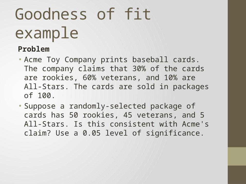
Goodness of fit example

Problem• Acme Toy Company prints baseball cards. The company claims

that 30% of the cards are rookies, 60% veterans, and 10% are All-Stars. The cards are sold in packages of 100.

• Suppose a randomly-selected package of cards has 50 rookies, 45 veterans, and 5 All-Stars. Is this consistent with Acme's claim? Use a 0.05 level of significance.

Using Excel to find • Determine

• Create 2 columns: n and p, and enter appropriate values• In the 3rd column:

n p E sub i100 0.6 60100 0.3 30100 0.1 10

Using Excel to find • Determine

• Add a 4th column to the spreadsheet: • In the 5th column, calculate each element of the statistic

• =(D2-C2)^2/C2• Sum the values of the 5th column

• This is the value, the test statistic

• Use the calculator to find the value of p, and interpret the test results.

n p E sub i O sub i100 0.6 60 45 3.75100 0.3 30 50 13.333100 0.1 10 5 2.50

19.583

Another G of F problem• Poisson Distribution• Automobiles leaving the paint department of an assembly

plant are subjected to a detailed examination of all exterior painted surfaces.

• For the most recent 380 automobiles produced, the number of blemishes per car is summarized below.

• Level of significance:

Blemishes 0 1 2 3 4

# of cars 242 94 38 4 2

Goodness-of-Fit: An Example• Problem 13.18: It has been reported that 10.3% of U.S.

households do not own a vehicle, with 34.2% owning 1 vehicle, 38.4% owning 2 vehicles, and 17.1% owning 3 or more vehicles. The data for a random sample of 100 households in a resort community are summarized below. At the 0.05 level of significance, can we reject the possibility that the vehicle-ownership distribution in this community differs from that of the nation as a whole?# Vehicles Owned # Households

0 201 352 233 or more 22

© 2011 Cengage Learning.All Rights Reserved. May not be scanned, copied, or duplicated, or posted to a publicly accessible website, in whole or in part.

Goodness-of-Fit: Problem 13.18, cont.

H0: p0 = 0.103, p1 = 0.342, p2 = 0.384, p3+ = 0.171

Vehicle-ownership distribution in this community is the same as it is in the nation as a whole.

H1: At least one of the proportions does not equal the stated value. Vehicle-ownership distribution in this community is not the same as it is in the nation as a whole.


Goodness-of-Fit: Problem 13.18, cont.

II. Rejection Region:a = 0.05df = k – 1 – m = 4 – 1 – 0 = 3

III. Test Statistic:c2 = 16.7338

IV. Conclusion: Since the test statistic of c2 = 16.7338 falls well above the critical value of c2 = 7.815, we reject H0 with at least 95% confidence.

V. Implications: There is enough evidence to show that vehicle ownership in this community differs from that in the nation as a whole.

0.050.95

Do Not Reject H0 Reject H0

c =7.8152


Test for homogeneity• Single categorical variable from 2 populations

• Test if frequency counts are distributed identically across both populations

• Example: Survey of TV viewing audiences. Do viewing preferences of men and women differ significantly?

• We make the same assumptions we did for the goodness of fit test• Data is collected from a simple random sample (SRS)• Population is at least 10 times larger than sample• Variable is categorical• Expected value for each level of the variable is at least 5

• We use the same approach to testing

State the hypothesis• Data collected from r populations• Categorical variable has c levels• Null hypothesis is that each population has the same

proportion of observations, i.e.:H0: Plevel 1, pop 1 = Plevel 1, pop 2 =… = Plevel 1. pop r

H0; Plevel 2, pop 1 = Plevel 2, pop 2 - … = Plevel 2, pop r

…H0: Plevel c, pop 1 = Plevel c, pop 2=…=Plevel c, pop r

• Alternative hypothesis: at least one of the null statements if false

Analyze the sample data• Find

• Degrees of freedom• Expected frequency counts• Test statistic ()• p-value or critical value

Analyze the sample data• Degrees of freedom

• d.f.=(r-1) x (c-1)• Where

• r= number of populations• c= number of categorical values

Analyze the sample data• Expected frequency counts

• Computed separately for each population at each categorical variable

• Where:• = expected frequency count of each population• = number of observations from each population• = number of observations from each category/treatment level

Analyze the sample data• Determine the test statistic

• Determine the p-value or critical value

Test for homogeneity

Problem• In a study of the television viewing habits of children, a

developmental psychologist selects a random sample of 300 fifth graders - 100 boys and 200 girls. Each child is asked which of the following TV programs they like best.

Family Guy South Park The Simpsons Total

Boys 50 30 20 100

Girls 50 80 70 200

Total 100 110 90 300

State the hypotheses• Null hypothesis: The proportion of boys who prefer Family Guy is

identical to the proportion of girls. Similarly, for the other programs. Thus:H0: Pboys who like Family Guy = Pgirls who like Family Guy

H0: Pboys who like South Park = Pgirls who like South Park

H0: Pboys who like The Simpsons = Pgirls who like The Simpsons

• Alternative hypothesis: At least one of the null hypothesis statements is false.

Analysis plan• Compute

• Degrees of freedom• Expected frequency counts• Chi-square test statistic

• Degrees of freedom

• Where:• = number of population elements• = number of categories/treatment levels

• In this case

Analysis plan

Compute the expected frequency countsEr,c = (nr * nc) / nE1,1 = (100 * 100) / 300 = 10000/300 = 33.3E1,2 = (100 * 110) / 300 = 11000/300 = 36.7E1,3 = (100 * 90) / 300 = 9000/300 = 30.0E2,1 = (200 * 100) / 300 = 20000/300 = 66.7E2,2 = (200 * 110) / 300 = 22000/300 = 73.3E2,3 = (200 * 90) / 300 = 18000/300 = 60.0


Boys 50 30 20 100

Girls 50 80 70 200

Total 100 110 90 300

Analysis plan• Determine the test statistic


Boys 50 (33.3) 30 (36.7) 20 (30.0) 100

Girls 50 (66.7) 80 (73.3) 70 (60.0) 200

Total 100 110 90 300

Analysis plan• p-value

• use the Chi-Square Distribution Calculator to find P(Χ2 > 19.91) = 1.0000


Test for independence• Almost identical to test for homogeneity

• Test for homogeneity: Single categorical variable from 2 populations

• Test for independence: 2 categorical variables from a single population

• Determine if there is a significant association between the 2 variables

• Example• Voters are classified by gender and by party affiliation (D,R,I). • Use X2 test to determine if gender is related to voting preference

(are the variables independent?)

Test for independence• Same assumptions• Same approach to testing• Hypotheses

• Suppose variable A has r levels and variable B has c levels. The null hypothesis states that knowing the level of A does not help you predict the level of B. The variables are independent.

• H0: Variables A and B are independent

• Ha: Variables A and B are not independent• Knowing A will help you predict B

• Note: Relationship does not have to be causal to show dependence

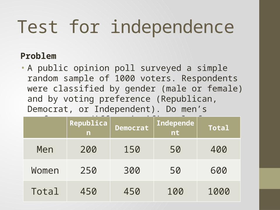
Test for independence

Problem• A public opinion poll surveyed a simple random sample of

1000 voters. Respondents were classified by gender (male or female) and by voting preference (Republican, Democrat, or Independent). Do men’s preferences differ significantly from women’s?

Republican Democrat Independent Total

Men 200 150 50 400

Women 250 300 50 600

Total 450 450 100 1000

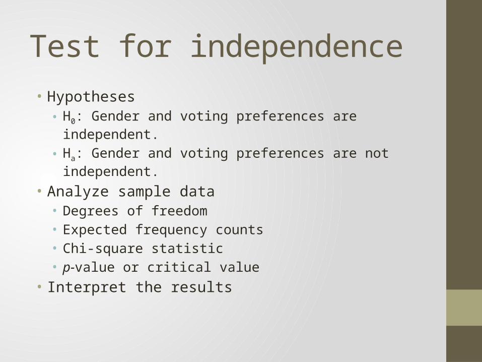
Test for independence• Hypotheses

• H0: Gender and voting preferences are independent.

• Ha: Gender and voting preferences are not independent.

• Analyze sample data• Degrees of freedom• Expected frequency counts• Chi-square statistic• p-value or critical value


Chi-Square Tests of Independence

An Example, Problem 13.35: Researchers in a California community have asked a sample of 175 automobile owners to select their favorite from three popular automotive magazines.

Of the 111 import owners in the sample, 54 selected Car and Driver, 25 selected Motor Trend, and 32 selected Road & Track. Of the 64 domestic-make owners in the sample, 19 selected Car and Driver, 22 selected Motor Trend, and 23 selected Road & Track.

At the 0.05 level, is import/domestic ownership independent of magazine preference? Based on the chi-square table, what is the most accurate statement that can be made about the p-value for the test?


Chi-Square Tests of Independence

• First, arrange the data in a table. Car and Motor Road & Driver (1) Trend (2) Track (3)

Totals Import (Imp) 54 25 32 111 Domestic (Dom) 19 22 23

64 Totals 73 47 55

175• Second, compute the expected values and contributions to c2 for

each of the six cells.• Then to the hypothesis test.... © 2011 Cengage Learning.

All Rights Reserved. May not be scanned, copied, or duplicated, or posted to a publicly accessible website, in whole or in part.

Chi-Square Tests of Independence• I. Hypotheses:

H0: Type of magazine and auto ownership are

independent.H1: Type of magazine and auto ownership are not

independent.• II. Rejection Region:

a = 0.05df = (r – 1) (k – 1) = (2 – 1)• (3 – 1) = 1 • 2 = 2

If c2 > 5.991, reject H0.0.050.95

Do Not Reject H0 Reject H0

c =5.9912


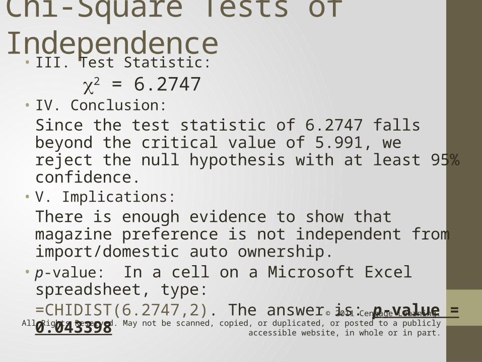
Chi-Square Tests of Independence• III. Test Statistic:

c2 = 6.2747• IV. Conclusion:

Since the test statistic of 6.2747 falls beyond the critical value of 5.991, we reject the null hypothesis with at least 95% confidence.

• V. Implications:There is enough evidence to show that magazine preference is not independent from import/domestic auto ownership.

• p-value: In a cell on a Microsoft Excel spreadsheet, type:=CHIDIST(6.2747,2). The answer is: p-value = 0.043398


chi-square distributions. recap analyze data and test hypothesis type of test depends on: data...

Documents

independence slide

cars242943842 slide

fdistribution slide

cumulative probability

chisquare distributions

goodness of fit test

vehicleownership distribution

homogeneity test