Chi Square and t-testsPresented by

Group C

Introduction

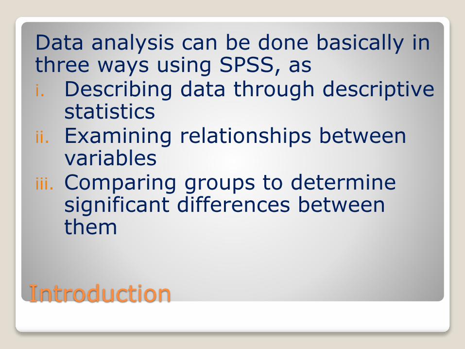
Data analysis can be done basically in three ways using SPSS, asi. Describing data through descriptive

statisticsii. Examining relationships between

variablesiii. Comparing groups to determine

significant differences between them

Introduction

Considering the third category i.e. comparing groups, chi square and t-tests are two of the important tests. These are tests of significance.

Chi-Square Test

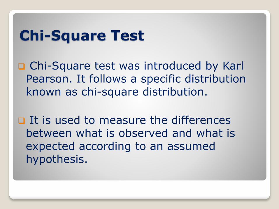
Chi-Square test was introduced by Karl Pearson. It follows a specific distribution known as chi-square distribution.

It is used to measure the differences between what is observed and what is expected according to an assumed hypothesis.

Chi-Square Test

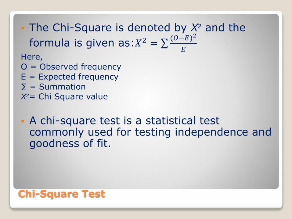
The Chi-Square is denoted by X² and the

formula is given as:𝑋2 = (𝑂−𝐸)2

𝐸Here,

O = Observed frequency

E = Expected frequency

∑ = SummationX²= Chi Square value

A chi-square test is a statistical test commonly used for testing independence and goodness of fit.

Chi-Square Test

Testing independence determines whether two or more observations across two populations are dependent on each other (i.e., whether one variable helps to estimate the other). If the calculated value is less than the table value at certain level of significance for a given degree of freedom, we conclude that null hypotheses stands which means that two attributes are independent or not associated. If calculated value is greater than the table value, we reject the null hypotheses.

Chi-Square Test

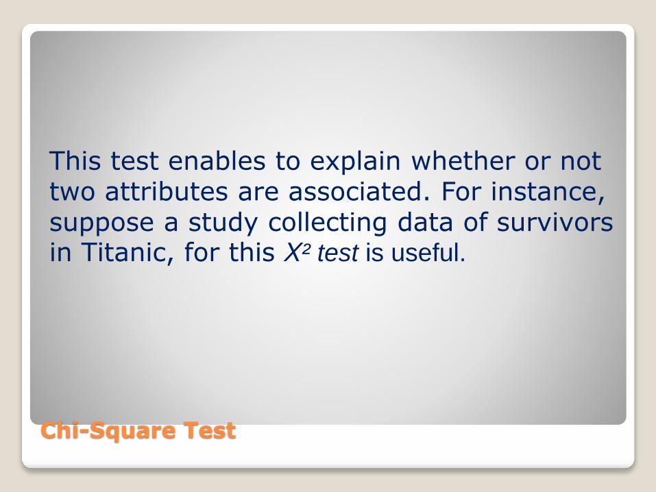
This test enables to explain whether or not two attributes are associated. For instance, suppose a study collecting data of survivors in Titanic, for this X² test is useful.

Chi-Square Test

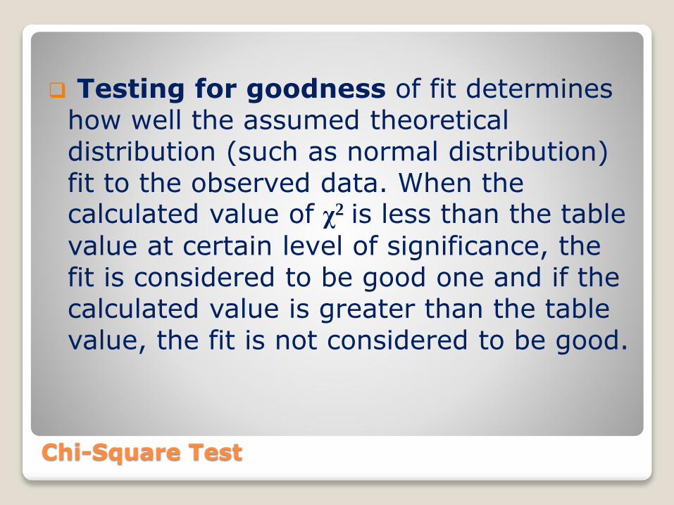
Testing for goodness of fit determines how well the assumed theoretical distribution (such as normal distribution) fit to the observed data. When the calculated value of χ2 is less than the table

value at certain level of significance, the fit is considered to be good one and if the calculated value is greater than the table value, the fit is not considered to be good.

Let’s explain its use in SPSS with the help of an example

Chi-Square in SPSS

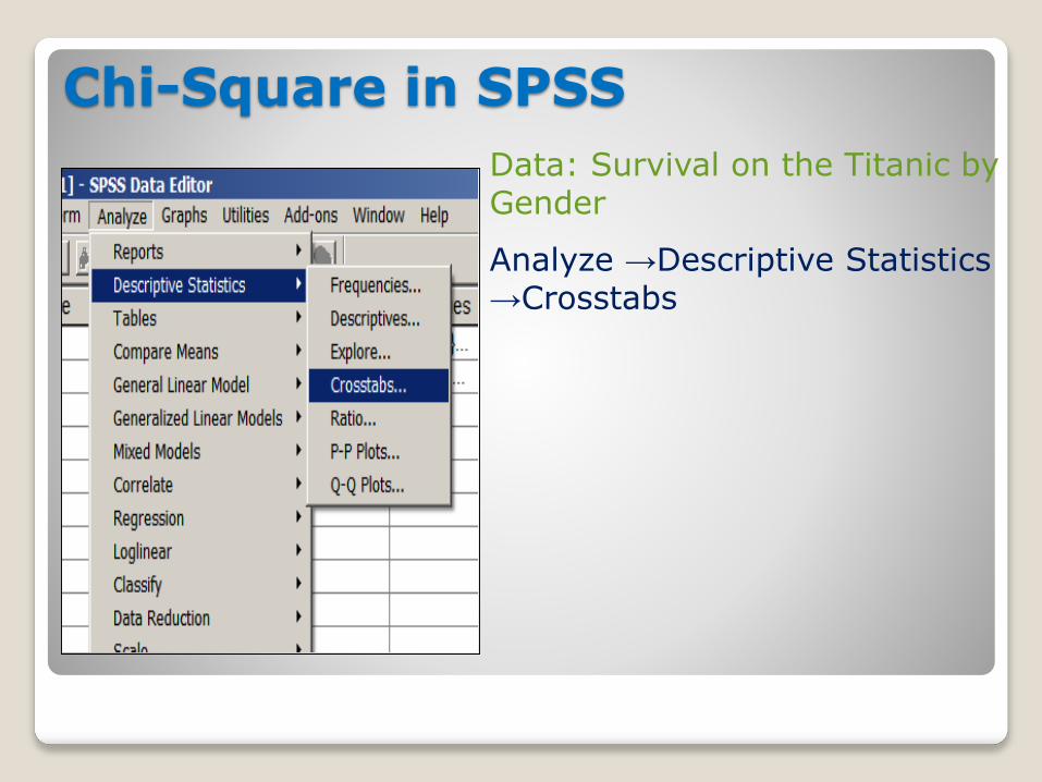
Data: Survival on the Titanic by Gender

Analyze →Descriptive Statistics→Crosstabs

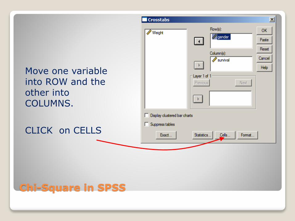
Chi-Square in SPSS

Move one variable into ROW and the other into COLUMNS.

CLICK on CELLS

Chi-Square in SPSS

Independent Variable (Gender) is in the Rows

Always show Observed count

Optionally, show Expectedcount

Percentage across the Rows

Click CONTINUE In main dialogue box,

Click STATISTICS

Chi-Square in SPSS

Choose Chi-Square for hypothesis test

Click Phi and Cramer’s V for measure of strength of the relationship

Click CONTINUE

On main dialogue box, Click OK

Chi-Square in SPSS

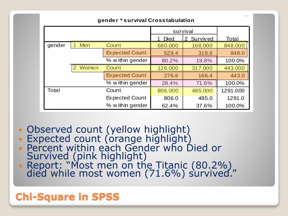
Observed count (yellow highlight) Expected count (orange highlight) Percent within each Gender who Died or

Survived (pink highlight) Report: “Most men on the Titanic (80.2%)

died while most women (71.6%) survived.”

gender * survival Crosstabulation

680.000 168.000 848.000

529.4 318.6 848.0

80.2% 19.8% 100.0%

126.000 317.000 443.000

276.6 166.4 443.0

28.4% 71.6% 100.0%

806.000 485.000 1291.000

806.0 485.0 1291.0

62.4% 37.6% 100.0%

Count

Expected Count

% w ithin gender

Count

Expected Count

% w ithin gender

Count

Expected Count

% w ithin gender

1 Men

2 Women

gender

Total

1 Died 2 Survived

survival

Total

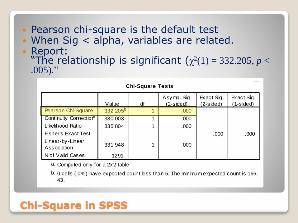
Chi-Square Tes ts

332.205b 1 .000

330.003 1 .000

335.804 1 .000

.000 .000

331.948 1 .000

1291

Pearson Chi-Square

Continuity Correctiona

Likelihood Ratio

Fisher's Exact Test

Linear-by-Linear

Association

N of Valid Cases

Value df

Asymp. Sig.

(2-s ided)

Exact Sig.

(2-s ided)

Exact Sig.

(1-s ided)

Computed only for a 2x2 tablea.

0 cells (.0%) have expected count less than 5. The minimum expected count is 166.

43.

b.

Chi-Square in SPSS

Pearson chi-square is the default test When Sig < alpha, variables are related. Report:

“The relationship is significant (χ2(1) = 332.205, p < .005).”

Sym metric Measures

.507 .000

.507 .000

1291

Phi

Cramer's V

Nominal by

Nominal

N of Valid Cases

Value Approx. Sig.

Not assuming the null hypothes is.a.

Using the asymptotic standard error assuming the null

hypothesis.

b.

Chi-Square in SPSS

Phi for 2x2 tables Cramer’s V for larger tables

Both range from 0 to 1 with 0 = no relationship

For df = 1◦ V = 0.10 is a small

effect◦ V = 0.30 is a

medium effect◦ V = 0.50 is a large

effect Report: “Gender

had a large effecton chance of survival for the Titanic passengers.”

t-test

The t-test is a basic test that is limited to two groups. For multiple groups, we should have to compare each pair of groups, for example with three groups there would be three tests (AB, AC, BC).

It is used to test whether there is significant difference between the means of two groups, e.g.:

Male v female Full-time v part-time

t-test

There are three types of t-tests as below

A one sample t-test: used when we want to know if there is a significant difference between a sample mean and a test value (known mean from a population or some other value to compare with sample mean), i.e. to compare the mean of a sample with population mean.

t-test

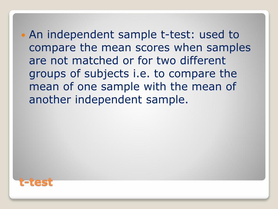
An independent sample t-test: used to compare the mean scores when samples are not matched or for two different groups of subjects i.e. to compare the mean of one sample with the mean of another independent sample.

t-test

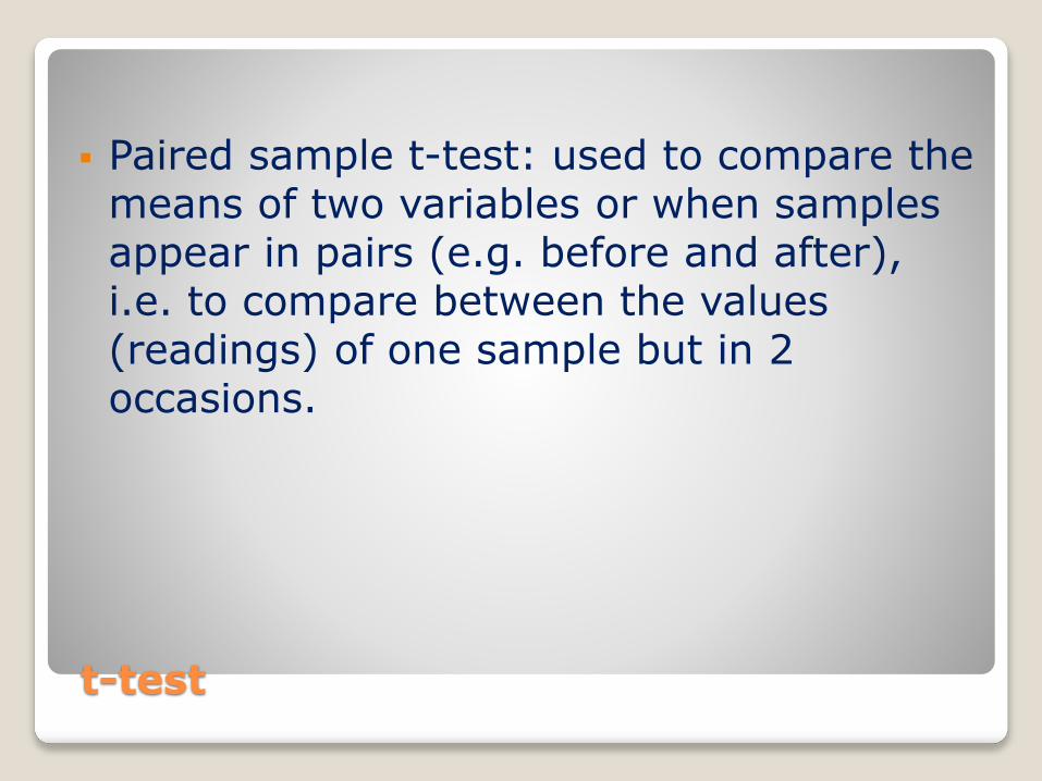
Paired sample t-test: used to compare the means of two variables or when samples appear in pairs (e.g. before and after), i.e. to compare between the values (readings) of one sample but in 2 occasions.

Let’s explain performing t-test in SPSS…

t-test in SPSS

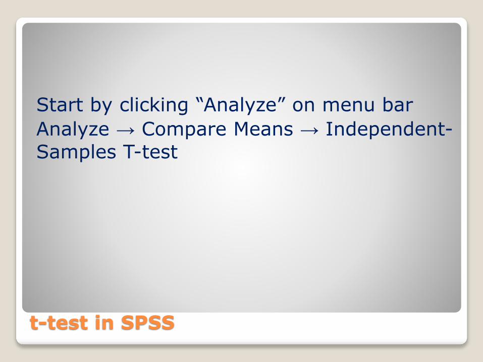
Start by clicking “Analyze” on menu bar

Analyze → Compare Means → Independent-

Samples T-test

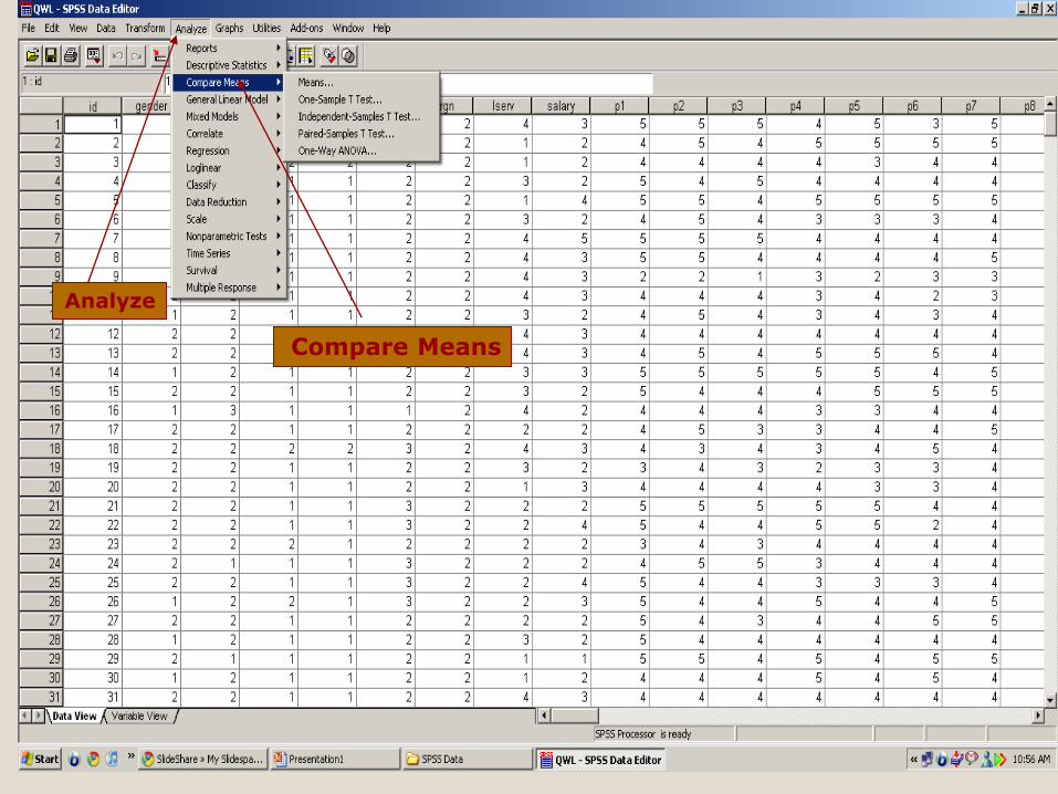
Compare Means

Analyze

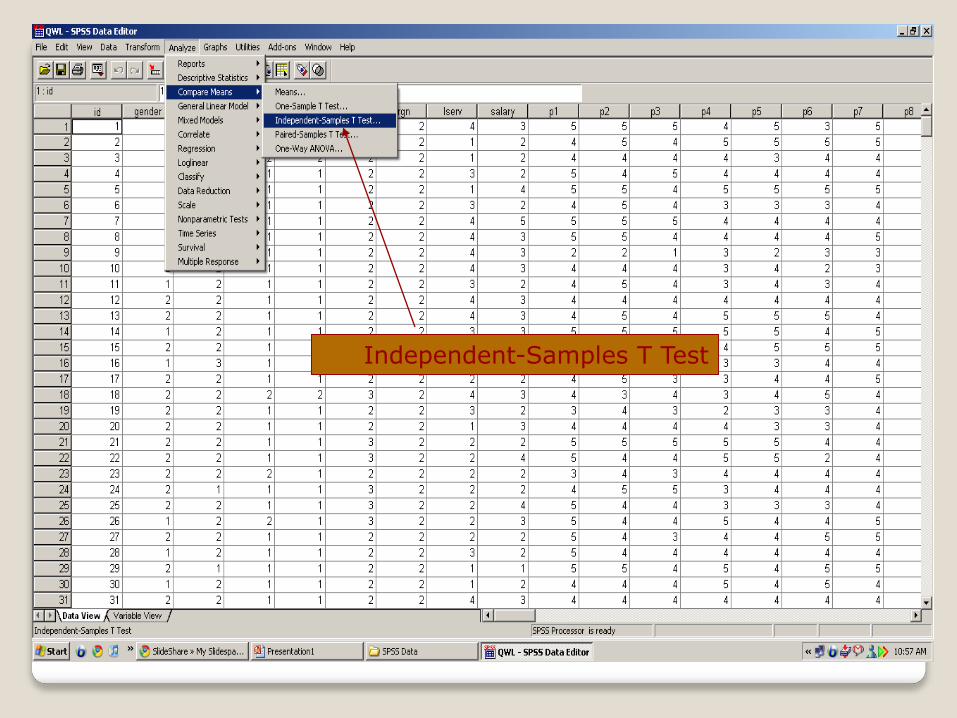
Independent-Samples T Test

t-test in SPSS

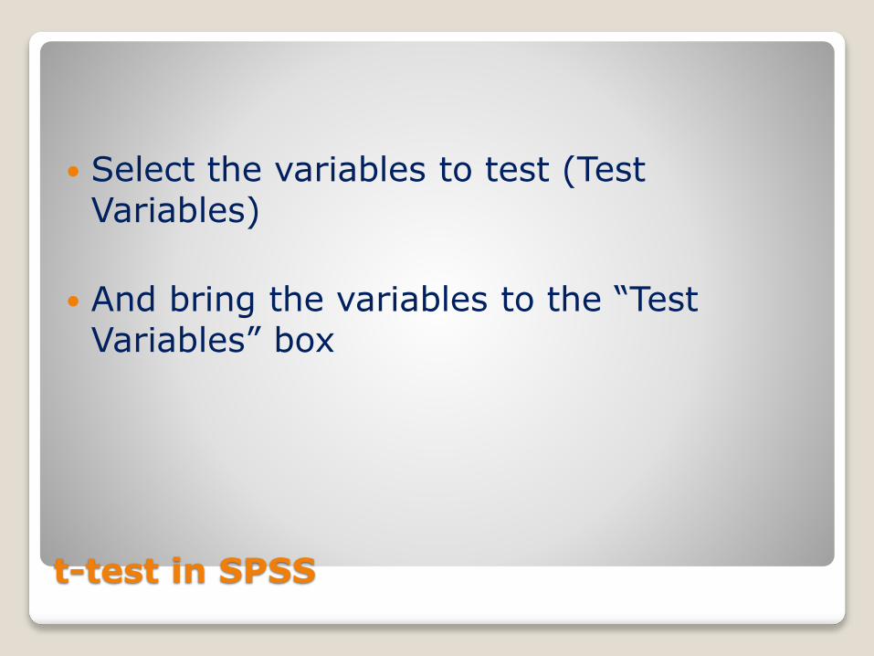
Select the variables to test (Test Variables)

And bring the variables to the “Test Variables” box

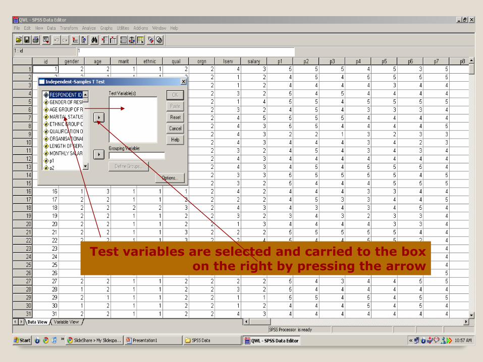
Test variables are selected and carried to the box on the right by pressing the arrow

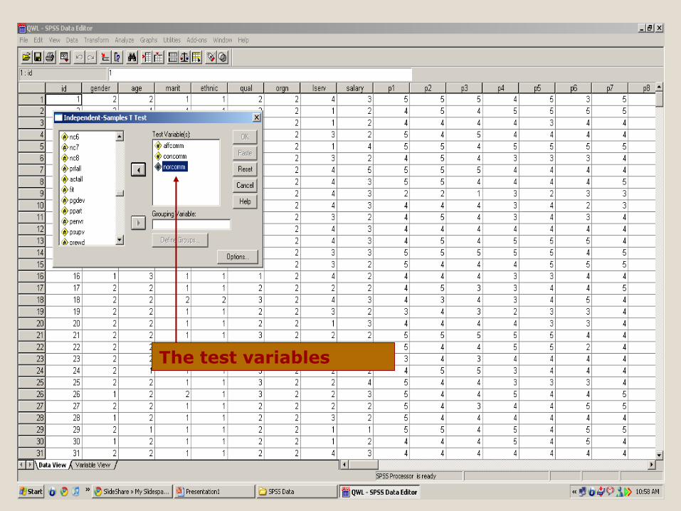
The test variables

t-test in SPSS

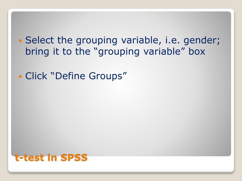
Select the grouping variable, i.e. gender; bring it to the “grouping variable” box

Click “Define Groups”

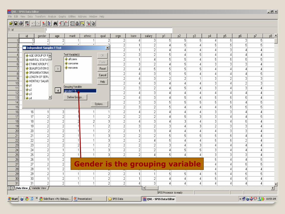
Gender is the grouping variable

t-test in SPSS

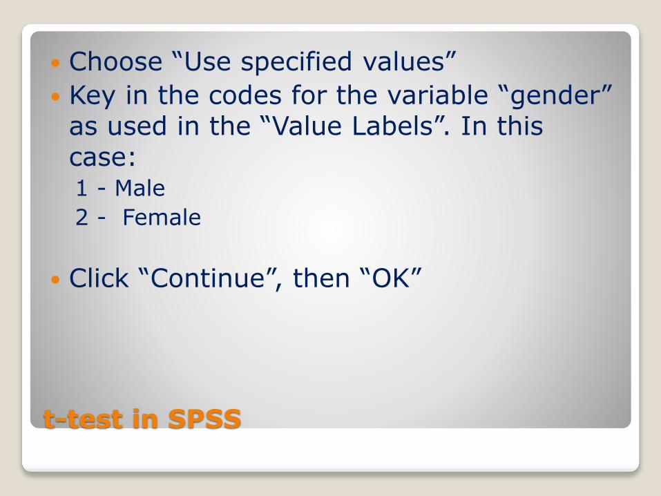
Choose “Use specified values”

Key in the codes for the variable “gender” as used in the “Value Labels”. In this case:1 - Male

2 - Female

Click “Continue”, then “OK”

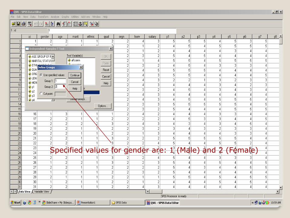
Specified values for gender are: 1 (Male) and 2 (Female)

For t-test interpretation lets switch to SPSS

The End