Facial Feature Addition and Alteration

Tony Chen

Department of Bioengineering

Stanford University

Stanford, CA, USA

tchen87@gmail.com

While face and facial feature detection is an important and

popular problem in image processing and algorithm

development, the work presented here is far less important. Here I attempt to build on existing methods of face detection and facial

feature detection in order to automate and customize an old

practical joke where one scribbles facial hair onto a picture of

friends, celebrities, or even complete strangers. Using the

OpenCV Viola-Jones Face Detection algorithm and a modified chin and cheek contour detection method, key locations on the

face are defined for use in drawing photorealistic facial hair on

an image. A skin detection algorithm is also used in order to

segment out and remove real facial hair and replace it with

photorealistic skin.

Keywords: facial feature detection, contour detection, face

alteration

I. INTRODUCTION

The face is one of the most important identifying

characteristics for a person. As such, face recognition and

detection algorithms have been the subject of hundreds of

research papers, and algorithms have been designed for

commercial use in digital cameras and phones. Going even

further from simply detecting the face, there is now great

interest in examin ing the details of a person’s facial features

and trying to ext ract information from them. There are many

uses for this sort of data, including physiognomic analysis [1],

emotion ext raction [2], and feature tracking in v ideophones

[3]. There is also some interest in being able to alter facial

features, again for various reasons including the simulation of

age [4].

This work attempts to apply known techniques for face

detection and facial feature detection to a less practical and

more entertaining purpose. The scribbled addition of facial

hair to portraits of other people is a long standing joke played

by kids everywhere. In an attempt to provide a d igital version,

the joke is implemented as a MATLAB GUI to give the user

control over what type of facial hair to bestow on an input

image with a face in it. An OpenCV Vio la-Jones Face

Detection algorithm [5] is used to determine the location of the

eyes, nose, and mouth of the face in the image. Based on these

points, average human face proportions, image gradients, and

edge detection, the contours defining the chin and cheek

boundaries of the face are then identified. Using these

contours as guidelines, important points on the face are plotted

for use in painting hair on the image. The hair color used in

the fake facial hair is extracted from the person’s actual hair.

The GUI can also remove facial hair and glasses from the

person’s face, replacing the area with skin colored pixels.

II. DESCRIPTION OF ALGORITHMS

A. Face Detection and Facial Feature Localization

An MATLAB implementation of the OpenCV Viola Jones Face Detection is used in this project [5]. The result is the

approximate location and scale of the face, shown in figure 1B. Following face detection and included in this implementation is

a facial feature localization algorithm. This algorithm utilizes a probability distribution using a multiple Gaussian tree

structured covariance to search for the feature positions using

distance transform methods [6]. Then, a feature/non-feature classifier is used to locate the left and right corners of each eye,

the two nostrils and the tip of the nose, and the left and right corners of the mouth, also shown in figure 1B.

B. Chin and Cheek Contour Detection

The framework for detecting the chin and cheek contours

that define the borders of the face is an adaptation of the work

done by Markus Kampmann [7] [8]. The points defining these contours are derived using the facial landmarks detected

previously, knowledge regarding the proportions of the average human face (figure 2), and magnitude of the gradient of the

image. The ch in and cheek contours are composed of four

Figure 1: Face detection and Facial Feature Localization

(A) Input Image (B) Face region detected within the yellow

square, facial features detected as yellow crosses

A B

parabolas which can be defined by five points (figure 3). A is

the bottom of the chin, and the vertex of two parabolas connecting A to B and A to C. B is the right chin point, while C

is the left chin point. These two points serve as the vertices for parabolas connecting B to D, and C to E, where D and E are

the right and left cheek points, respectively.

The first step is to find point A. As a first pass, point A

must lie along the axis connecting the point centered between the eyes and the center of the mouth, defined as l1 (see figure

4). If the distance between the center of the eyes and the center of the mouth is x, then the bottom of the chin was assumed to

be a distance 2x away from the point between the eyes along l1.

This is where the search for A is centered. The bounds a1 and a2 (Figure 4) also lie on this axis and are roughly 0.33x away

from the starting point in either direction. All the points between a1 and a2 are then given a probability based on their

distance from the center. The probability is defined by a

Gaussian centered around the starting point and with a sigma

calculated from the number of points within a1 and a2. Then, the magnitude of the image gradient (calculated using the Sobel

method from the luminance component of the image in YCbCr

space) for each of the points is also calculated. These gradient values were normalized from zero to one, and then weighted

twice as much as the distance probability values. The two measures were added together, and the point with the highest

value was defined to be A.

A similar strategy was used for defining points B and C.

The reference distance x in this case is the width of the mouth.

For the first pass, points B and C both had to lie on the axis connecting the left and right ends of the mouth (l2 in figure 4).

Gaussians for the distance probability metric were centered on a point 0.4x away from each end of the mouth. The boundaries

b2 and c1 were placed 0.16x away from their respective ends of the mouth, and the boundaries b1 and c2 were a distance x

away from their ends of the mouth. The values of the gradient image within these borders were extracted and normalized as

before, but with no extra weighting. At this point, the

probability that the point was skin colored was also taken into account, and weighted twice as high as the other values. This

was done to prevent high gradient objects in the background from overwhelming the metrics. All the values for each pixel

were then added up, and those points that maximized these metrics were defined to be B and C. Finally, if the pixel next to

B or C in the direction away from the mouth had a skin

probability greater than 70%, the chin point was moved to that pixel until this condition no longer held true. This

implementation helped to get away from parts of the face that had large gradient magnitudes, such as smile lines. The skin

color segmentation will be described in a later section.

With initial positions for A, B, and C, a second pass was

done to refine the locations of these points. First, point A was

adjusted. The point was no longer restricted to the l1 line. A square area around the initial A position was searched with the

following methodology: for each position, a parabola connecting A to B and A to C was generated, with A as the

vertex in both cases. The mean magnitude of the gradient image along these parabolas was calculated for each tested

position. The distance from the original A point was also calculated for each test point, with greater distance from the

original point having less probability. After calculating these

metrics for all the test points, the matrices were normalized

Figure 4: Chin Contour detection [7] First pass set up.

Figure 3: Deformable template for chin and cheek

contours [7]

Figure 2: Average Human Face proportions, courtesy

of http://maiaspaintings.blogspot.com/

from 0 to 1 and added together. The point with the maximum

value was selected to be the final A point.

A similar method was used to calculate the second pass

positions for B and C. The points were no longer restricted to be on the l2 line. A square area around the initial positions

were tested for each of B and C, and for each position the distance from the original point was calculated, the mean

gradient of the parabola between the test point and the new A

point was calculated, and the skin probability of the test point was calculated. These matrices were again normalized from 0

to 1, added together, and the point with the maximum value was selected as the final B and C points. Figure 5 shows the

results.

The last step was to find the points defining the cheeks, D and E. As a first pass, these points had to lie on the line l4,

which is parallel to the line connecting the centers of the eyes l3. The distance g between l4 and l3 (figure 6) was defined as

half the distance between the point between the eyes and the tip of the nose. The same method for defining the first passes of

points B and C was used here, with the reference distance x

being half the distance between the outermost edges of the left and right eyes. The inner boundaries d2 and e1 were x away

from the intersection of l1 and l4, and the outer boundaries d1 and e2 were 2x away from the intersection of l1 and l4. The

Gaussian probability was centered halfway in between the boundaries, and the weightings for gradient magnitude and skin

probability were the same as for B and C. The second pass

methodology for D and E was also the same as for B and C, with the skin probability, distance from the orig inal point, and

mean gradient value along the parabolas connecting B to D and C to E (with B and C as the vertices) being calculated for a

square area around the original points.

C. Skin Color Extraction and Segmentation

Two methods of skin color segmentation were used, each

with a different purpose. The first method was adapted from

[8] and utilized a broad model for skin color. Non-parametric

histogram-based models were trained using manually

annotated skin and non-skin pixels, and the log likelihood of a

pixel being skin or non-skin was calculated from these

histograms. A normalized version of the result was used in the

second pass detection of points B-E as described above. An

example of this algorithm at work is shown in figure 7.

The second skin detection algorithm was implemented

more specifically to a given test image, and was adapted from

[9]. Rather than using a broad model trained on many different

skin tones, sections of the test image directly below the eyes

but above the mouth (see figure 8A) were cut out and used as

the template for skin co lor. These sections were converted

from RGB to YCbCr, and the Cb and Cr values were

extracted. These sections underwent a low pass filter to reduce

the effect of noise, and the indiv idual pixel values were then

binned in chromatic color space, where the mean and

covariance were calculated and used to fit a Gaussian

distribution to the data. Based on this Gaussian, the likelihood

of any pixel in the image being skin could be calculated. A

normalized version of these likelihoods was used when

extending the first pass versions of points B-E to the edge of

the face. An example of the segmentation results can be seen

in figure 8B. While the results shown for the test image are

quite good, because of the small sa mple size of the input skin

template, the results were typically more inconsistent than the

broad skin color segmentation described previously.

Figure 7: Broad, manually trained skin detection algorithm

based on RGB histograms.

Figure 6: Cheek contour detection [7] First pass set

up.

Figure 5: Chin Point Detection Algorithm. The green

points show first pass detection, and the red points show

the adjustments made in the second pass. Point B was

correct on the first pass, so the second pass did not change

it.

D. Hair Color Extraction and Painting of facial hair

In order to paint photorealistic facial hair onto a given face

image, the actual color of the person’s hair was extracted. This

was done using the results of the second, more specific skin

segmentation algorithm. An elliptical mask was generated

around the detected face using previously detected points as

guidelines, and this mask was multip lied with a threshholded

version of the inverse skin probability in order to find the

regions within the ellipse that were probabilistically not skin.

The topmost region in this mask was defined to be hair, and

the pixels within this region were smoothed with a low pass

filter to reduce noise. The results of this extract ion are shown

in figure 9.

Painting hair on the face involved generating a number of

points on the face in relevant locations, then connecting these

points with parabolas or lines in interesting ways. The points

were generated using the baseline facial feature points

detected in part A, as well as the dimensions of the detected

face. Some of these points are shown in figure 10. These

segments formed the borders of a polygon representing a

facial hair style, and the points making up these borders were

used as vertices for triangles that traversed the resulting

polygon. Each of the triangles was filled with a random co lor

picked from the pixels defined to be hair in the method

described previously.

E. Facial Hair and Glasses Removal

Because of the variability in shape and color of facial hair

and glasses, it was difficult to sculpt an algorithm that would

perfectly remove the facial hair or g lasses from any given

face. The algorithm used in this implementation involves a

mask that completely covers the region in which there might

be facial hair or g lasses, and replaces it with photorealistic

skin. The masks were generated using facial feature points,

and the painted skin is generated from the rectangles extracted

for the second skin segmentation algorithm prev iously

described.

In order to smooth out the transition between the original

image and the replaced skin p ixels, an image inpainting

algorithm was used [10]. Using image dilation and erosion, the

borders of the mask were defined, and the inpainting algorithm

interpolated the values within this border region between the

replaced skin pixels and the original image. Examples of this

algorithm are shown in figure 12 in the results section.

III. RESULTS

A Graphical User Interface (GUI) was created in MATLAB to implement all of the methods and algorithms described. The

layout of the GUI is shown in figure 11. There were 11 facial hair styles that were implemented using the methods described

above. Moustaches could be added in the style of Mario, Zorro, Hulk Hogan, Einstein, and Fu Manchu, as well as the more

standard handlebar moustache. Beards could be added as a soul

patch, a goatee, a chin puff, a scraggly beard, or in the style of Jack Sparrow. These could also be combined together to form

new styles. Examples of each of these styles, as well as the removal of facial hair and glasses are shown in figure 12.

Addition of glasses was also added to complement the removal of glasses feature.

Figure 10: Points used for painting facial hair. These

points were defined using the original 9 detected facial

feature points, as well as the points defined during chin

and cheek contour detection.

Figure 9: Hair color extraction. (A) The ellipse used to

segment out the face. (B) The topmost region of pixels not

reaching the skin threshold.

Figure 8: Skin Detection Algorithm specific to a given

image. (A) The white rectangles show the areas of skin that

are fed into the algorithm as template. (B) The results of

the segmentation.

A B A B

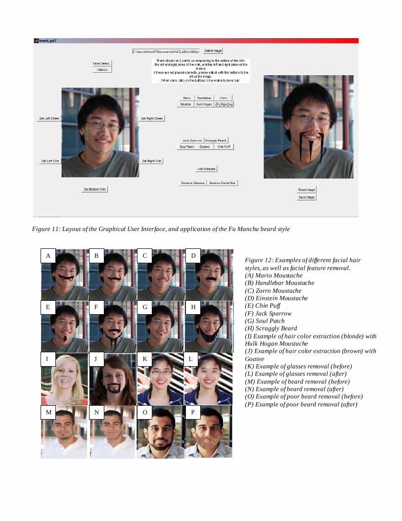
Figure 11: Layout of the Graphical User Interface, and application of the Fu Manchu beard style

Figure 10: Layout of the Graphical User Interface, and application of the Fu Manchu beard style

Figure 12: Examples of different facial hair

styles, as well as facial feature removal.

(A) Mario Moustache

(B) Handlebar Moustache

(C) Zorro Moustache

(D) Einstein Moustache

(E) Chin Puff

(F) Jack Sparrow

(G) Soul Patch

(H) Scraggly Beard

(I) Example of hair color extraction (blonde) with

Hulk Hogan Moustache

(J) Example of hair color extraction (brown) with

Goatee

(K) Example of glasses removal (before)

(L) Example of glasses removal (after)

(M) Example of beard removal (before)

(N) Example of beard removal (after)

(O) Example of poor beard removal (before)

(P) Example of poor beard removal (after)

A B C D

E F G H

I J K L

O P M N

There were several features added to the GUI for ease of

use. The user can select an image from anywhere in the file directory to upload into the GUI. In the case of multiple faces

in the same picture, the user can select which face to add facial hair to. If the points detected for the cheek and chin contours

are slightly off, the user can adjust the points in order to facilitate better results when adding facial hair or removing

facial features. Finally, the user can save the resultant image for

posterity.

IV. DISCUSSION

The chin and cheek contour detection strategy works fairly

well in spite of variability between persons in facial structure,

as well as differences in backdrops and rotation angle of the face. However, the strategy is not perfect, particularly when the

background has a color very similar to the skin tone of the face in question. It also tends to fail when the facial points detected

by the OpenCV Vio la Jones framework are off the mark. Because the first pass detection of the key points in the contour

are must lie on axes that are defined by the detected facial

points, if, say, the left edge of the mouth is detected incorrectly, then the algorithm will search for B and C on the wrong axis.

The second pass search helps to mitigate this effect, but problems can still occur. This is why the ability to let the user

specify the points manually was implemented into the GUI. Another problem with the strategy is the fact that the contours

were restricted to parabolic curves. In fact, a higher order polynomial (4

th order) might be warranted to account for more

blocky facial contours. Further work to make the algorithm

more robust might include Active Shape Modeling [11]. Th is method utilizes statistical models of object shapes through

manually labeled training sets in order to find similar shapes in a given test image.

Regarding the removal of facial hair and glasses, there were several problems encountered. Initially, the algorithm only

replaced pixels within the chin or eye mask that were classified

as not skin by the previously described skin segmentation routines. One problem with this was that the borders of the

facial hair tended to be close enough to skin color to fall within the skin threshold. This problem was exacerbated for people

with darker skin color and thus dark facial hair. In these cases, the skin segmentation had a hard time differentiating between

the two. The other main problem encountered was

inhomogeneous lighting, where one side of the face was brighter than the other. In this case, the skin segmentation was

even poorer due to the larger variance of skin tones, and large parts of the face would be incorrectly classified as skin or not

skin. The quick solution to this was to replace the entire region with new skin, rather than just the not skin areas. While this

tended to work better (figure 12N) it was still not robust to the differences in lighting, as seen in Figure 12O and 12P. Because

the lighting was so much brighter on the left side of the image,

the replaced skin appears much darker than it should be, and similarly on the right side, the skin appears brighter than it

should. The correction of this effect is an active area of research, and future work that makes use of the various models

of illumination, such as the one proposed in [12], could help to make the removal of glasses and facial hair more robust.

V. CONCLUSION

While the real life scribbling of facial hair on a picture is

quite simple, it turns out that carrying out the same process

digitally involves many steps, including face detection, facial

feature detection, skin segmentation, and hair color ext raction.

Even more d ifficu lt is the removal of facial hair and glasses,

which requires all of the above as well as image inpainting.

There are some problems with the implementation as it is, but

the problems are well known and have been addressed in other

work. Applying some of the techniques described in [11] and

[12] could make the practical joke even more robust and

entertaining.

ACKNOWLEDGMENT

I would like to thank Huizhong Chen for being my mentor

and providing advice and encouragement for the duration of my time working on the project. I would also like to thank

David Chen and Professor Bernd Girod for teaching a wonderfully entertaining and useful class. Finally, I would like

to thank all the Bioengineering students who graciously let me

use their faces as guinea pigs.

REFERENCES

[1] Hee-Deok Yang and Seong-Whan Lee. “Automatic Physiognomic

Analysis by Classifying Facial Component Feature,” 18th International Conference on Pattern Recognition (ICPR 2006), pp 1212, 2006.

[2] Kwang-Eun Ko and Kwee-Bo Sim. “Development of the facial feature extraction and emotion recognition method based on ASM and Bayesian Network,” IEEE International Conference on Fuzzy Systems, pp2063, 2009.

[3] Zhiwei Zhu and Qiang Ji. “Robust Pose Invariant Facial Feature Detection and Tracking in Real-Time,” 18th International Conference on Pattern Recognition (ICPR 2006), pp 1092, 2006.

[4] Lanatis, A., Taylor, C.J., Cootes, T .F. “Toward Automatic Simulation of Aging Effects on Face Images,” IEEE Transactions on Pattern Analysis and Machine Intelligence, pp 442, 2002.

[5] Everingham, M. , Sivic, J. and Zisserman, A. "Hello! My name is... Buffy" - Automatic Naming of Characters in TV Video ,” Proceedings of the British Machine Vision Conference. 2006.

[6] Markus Kampmann. “Estimationg of the Chin and Cheek Contours for Precise Face Model Adaptation,” International Conference on Image Processing, 1997.

[7] Markus Kampmann. “MAP Estimation of Chin and Cheek Contours in Video Squences,” EURASIP Journal on Applied Signal Processing , 6: pp 913-922. 2004.

[8] Ciarán Ó Conaire, Noel E. O'Connor and Alan F. Smeaton, "Detector adaptation by maximising agreement between independent data sources", IEEE International Workshop on Object Tracking and Classification Beyond the Visible Spectrum , 2007.

[9] Henry Chang and Ulise Robles. “Face Detection,” EE368 Final Project Report, 2000

[10] John D’Errico. “ inpaint_nans” (http://www.mathworks.com/matlabcentral/fileexchange/4551-inpaintnans), MATLAB Central File Exchange, 2006.

[11] Mahoor, Mohammad H. et al. “Improved Active Shape Model for Facial Feature Extaction in Color Images,” Journal of Multimedia, vol 1: 4 pp 21-28, 2006.

[12] Chen, Terrence, et al. “Total Variation Models for Varialbe Lighting Face Recognition,” IEEE Transactions on Pattern Analysis and Machine Intelligence, vol 28: 9, pp 1519-1524, 2006.