characterizing interference in wireless mesh networks
TRANSCRIPT

Characterizing Interference inWireless Mesh Networks
HUI, Ka Hung
A Thesis Submitted in Partial Fulfilmentof the Requirements for the Degree of
Master of Philosophyin
Information Engineering
c©The Chinese University of Hong Kong
August 2007
The Chinese University of Hong Kong holds the copyright of this thesis. Anyperson(s) intending to use a part or whole of the materials in the thesis ina proposed publication must seek copyright release from the Dean of theGraduate School.

Abstract of thesis entitled:Characterizing Interference in Wireless Mesh Networks
Submitted by HUI, Ka Hungfor the degree of Master of Philosophyat The Chinese University of Hong Kong in August 2007
The relationship between interference and capacity has been a
main focus in the study of wireless mesh networks. To find outthe capacity of a wireless mesh network, we have to accuratelymodel the interference among the wireless links. Then we can
design traffic engineering algorithms to allocate flows on eachlink to achieve the capacity.
Existing traffic engineering algorithms were designed basedon the celebrated interference model - protocol model, and the
existence of a perfect scheduler. However, these assumptionsonly help simplify the problem, and may not be achieved in
reality. Therefore, these works may have little value in currentwireless mesh networks.
In this thesis, we first introduce a new interference model -
partial interference, predicting the result of a transmission in awireless network to be probabilistic based on the corresponding
signal-to-noise ratio (SNR) and the modulation scheme used.We illustrate there is a gain in terms of capacity by considering
partial interference.Second, towards designing traffic engineering algorithms in
wireless random access networks, we study the stability regions
of 802.11 and slotted ALOHA networks under partial interfer-ence. The results show that the protocol model is not accurate
i

enough to model interference in a wireless network. By consid-ering partial interference, we show that the stability region is
larger, and the gain in network capacity can be provisioned.It is difficult to have a complete characterization on the sta-
bility regions of 802.11 and slotted ALOHA networks, as illus-trated in this thesis. Therefore, as a third contribution, wepropose FRASA, Feedback Retransmission Approximation for
Slotted ALOHA, as a surrogate to approximate the stability re-gion of slotted ALOHA. From this, we derive the convex hull
bound and the supporting hyperplane bound to outer-bound andinner-bound the stability region of FRASA respectively. These
bounds are guaranteed to be convex and piecewise linear. Byusing these bounds, the traffic engineering problem can be for-
mulated as linear programming, which can be solved by stan-dard techniques. We hope our work can serve as a basis in de-signing traffic engineering algorithms in wireless random access
networks.
ii

`
3PaçÏçÝ@~PaGr Wõç
Ýn;Î×Í@~ÝxP&Æmã@Ýÿl£
çd# ÝW0çQ¡&Æ|Ah
×ø;Õ°¼5gçÝø¼¾lïÝ
¨`Ýø;Õ°9ÎqA½(ÝWclÔ
ÜÈÿlõݼ×ݬ9°'©QÃ;
®Þ3¨@Îp|@¨ÝX|3¨ÝPaçÏç
@9°Õ°Ý®à¬
39¡Z&Æ´ñ×ͱÝGrWÿlÔI
5WÍPaçÝFíÎãXyãETÝ*r
¯f(SNR)CX¸àÝ×PXÝ^£&ƼA
&ÆÊPad# ÝI58çÞºÿÕè>
Íg Ý3Pa^Dãç'ø;Õ°
&Æ@~802.11C5ðALOHAç3I5WìÝ% ½îÜÈÿl¬ã@àçÝW
µ3ÊI5Wì&Æ|ÿÕ´Ý% ½yÎ
&ÆïÊI5Wñ¼çÝè>
&Ƽ0802.11C5ðALOHAÝ% ½
Î&ðæpÝyÎ&ÆèFRASAÔ5ðALOHAÝFDÿl¼ÿa5ðALOHA¬´O5ðALOHA% ½
Ý«ãh&Æß5½ãõYâø¿«X®ß
ÝFRASA% ½Ý²\&C/\&9ËÍ\&XWÝ
½KÎnðaPC«ÝDÄ9ËÍ\&&Æ|¿à
býã]°XÝaP!¼×ø;Õ°&Æ
T9¡Z® 'Pa^Dãçø;Õ°Ý
Í
iii

Acknowledgement
First of all, I would like to express my sincere gratitude to mysupervisors, Prof. Wing-Cheong Lau and Prof. On-Ching Yue,for their support and giving me freedom to explore interesting
research areas in these two years. Throughout these years, theiradvices, guidance, inspiration and patience have provided me
tremendous support. I wish to thank Prof. Jack Lee for hisadvices and suggestions in research group meetings.
I am grateful to Prof. Raymond Yeung, Prof. Peter Yumand my supervisors for writing reference letters and helping mein various applications.
I also thank all my friends, in particular, Wilson Ip, MichaelCheung, Jack Chan, Ryan Ho, Silas Fong and Derek Cheung, for
their help, support and entertainment. Thanks also to my newfriends in my graduate study: Ka-Ming Lau, Jack Chui, Gina
Yuen, Kin-Fai Li, Chun-Pong Luk, Deng Yun, Martin Choy,Terry Lo and Wing-Kai Lin, for their encouragement and shar-
ing of experiences in research and other areas.Finally, I want to give my wholehearted thankfulness for the
support, care and understanding from my family.
iv

This work is dedicated to my family and friends for their love
and support.
v

Contents
Abstract i
Acknowledgement iv
1 Introduction / Motivation 1
2 Literature Review 6
2.1 Introduction . . . . . . . . . . . . . . . . . . . . . 62.2 The Capacity-Finding Problem . . . . . . . . . . 62.3 Interference Models . . . . . . . . . . . . . . . . . 8
2.4 Considering Interference in the Capacity-FindingProblem with Perfect Scheduling . . . . . . . . . 9
2.4.1 Conflict Graph . . . . . . . . . . . . . . . 102.4.2 Independent Set Constraints . . . . . . . . 11
2.4.3 Row Constraints . . . . . . . . . . . . . . 112.4.4 Clique Constraints . . . . . . . . . . . . . 122.4.5 Using the physical model . . . . . . . . . . 13
2.5 Considering Interference in the Capacity-FindingProblem with Random Access . . . . . . . . . . . 15
2.6 Chapter Summary . . . . . . . . . . . . . . . . . 17
3 Partial Interference - Basic Idea 18
3.1 Introduction . . . . . . . . . . . . . . . . . . . . . 183.2 Deficiencies in Previous Models . . . . . . . . . . 18
3.2.1 Multiple Interferers . . . . . . . . . . . . . 19
vi

3.2.2 Non-binary Behavior of Interference . . . . 193.2.3 Impractical Perfect Scheduling . . . . . . . 21
3.3 Refining the Relationship between Interferenceand Throughput Degradation . . . . . . . . . . . 21
3.4 Capacity Gain by Exploiting Partial Interference . 233.5 Chapter Summary . . . . . . . . . . . . . . . . . 28
4 Partial Interference in 802.11 294.1 Introduction . . . . . . . . . . . . . . . . . . . . . 294.2 The 802.11 Model . . . . . . . . . . . . . . . . . . 29
4.2.1 Assumptions . . . . . . . . . . . . . . . . . 304.2.2 Transmission Probability Calculation . . . 31
4.2.3 Packet Corruption Probability Calculation 344.2.4 Loading Calculation . . . . . . . . . . . . 35
4.2.5 Summary . . . . . . . . . . . . . . . . . . 364.3 Some Analytical Results . . . . . . . . . . . . . . 374.4 A TDMA/CDMA Analogy . . . . . . . . . . . . . 40
4.5 Admissible (Stability) Region . . . . . . . . . . . 424.6 Chapter Summary . . . . . . . . . . . . . . . . . 44
5 Partial Interference in Slotted ALOHA 455.1 Introduction . . . . . . . . . . . . . . . . . . . . . 45
5.2 The Finite-Link Slotted ALOHA Model . . . . . . 465.2.1 Assumptions . . . . . . . . . . . . . . . . . 46
5.2.2 Stability of Slotted ALOHA . . . . . . . . 465.3 Stability Region of 2-Link Slotted ALOHA under
Partial Interference . . . . . . . . . . . . . . . . . 47
5.4 Some Illustrations . . . . . . . . . . . . . . . . . . 505.5 Generalization to the M -Link Case . . . . . . . . 53
5.6 Chapter Summary . . . . . . . . . . . . . . . . . 58
6 FRASA 59
6.1 Introduction . . . . . . . . . . . . . . . . . . . . . 596.2 The FRASA Model . . . . . . . . . . . . . . . . . 60
vii
6.3 Validation of the FRASA Model . . . . . . . . . . 666.3.1 Simulation Results . . . . . . . . . . . . . 66
6.3.2 Comparison to Previous Bounds . . . . . . 726.4 Convex Hull Bound . . . . . . . . . . . . . . . . . 75
6.5 p-Convexity . . . . . . . . . . . . . . . . . . . . . 806.6 Supporting Hyperplane Bound . . . . . . . . . . . 866.7 Extension to Partial Interference . . . . . . . . . 89
6.7.1 FRASA under Partial Interference . . . . . 906.7.2 Convex Hull Bound . . . . . . . . . . . . . 93
6.7.3 p-Convexity . . . . . . . . . . . . . . . . . 976.7.4 Supporting Hyperplane Bound . . . . . . . 101
6.8 Chapter Summary . . . . . . . . . . . . . . . . . 102
7 Conclusion and Future Works 110
7.1 Conclusion . . . . . . . . . . . . . . . . . . . . . . 1107.2 Future Works . . . . . . . . . . . . . . . . . . . . 111
A Proof of (4.13) in Chapter 4 113
Bibliography 123
viii

List of Figures
2.1 A connectivity graph and its corresponding con-flict graph [1]. . . . . . . . . . . . . . . . . . . . . 10
2.2 A counterexample for the unnecessity of row con-
straints [1]. . . . . . . . . . . . . . . . . . . . . . 122.3 A counterexample for the insufficiency of clique
constraints [1]. . . . . . . . . . . . . . . . . . . . . 14
3.1 Protocol model ignores the case of multiple inter-
ferers. . . . . . . . . . . . . . . . . . . . . . . . . 203.2 Throughput degradation and network separation. 233.3 A scheduling pattern in the modified Manhattan
network. . . . . . . . . . . . . . . . . . . . . . . . 243.4 Capacity across unit cut for different length of
links under the physical model (binary interfer-ence) and partial interference. . . . . . . . . . . . 26
4.1 A Markov chain model for 802.11 DCF in unsat-urated conditions. . . . . . . . . . . . . . . . . . . 32
4.2 A sample topology. . . . . . . . . . . . . . . . . . 384.3 Aggregate throughput for the topology in Fig. 4.2
with length of links = 450 meters and various
carrier sensing thresholds. . . . . . . . . . . . . . 404.4 Aggregate throughput for the topology in Fig. 4.2
with length of links = 400 meters and variouscarrier sensing thresholds. . . . . . . . . . . . . . 41
ix

4.5 A TDMA/CDMA analogy for the results in Sec-tion 4.3. . . . . . . . . . . . . . . . . . . . . . . . 42
4.6 Admissible region for various link separations. . . 43
5.1 A sample topology. . . . . . . . . . . . . . . . . . 51
5.2 Stability region for M = 2 with transmissionprobabilities 0.8 under binary and partial inter-ference. . . . . . . . . . . . . . . . . . . . . . . . 52
5.3 Stability region for M = 2 with link separation800 meters under binary and partial interference. 52
5.4 Stability region for M = 2 under binary interfer-ence and partial interference with various trans-
mission probabilities. . . . . . . . . . . . . . . . . 535.5 Stability region with M = 3. . . . . . . . . . . . . 57
6.1 Slotted ALOHA model: (Upper) Original; (Lower)FRASA. . . . . . . . . . . . . . . . . . . . . . . . 61
6.2 Stability region with M = 2: (Upper) From [2];
(Lower) From FRASA. . . . . . . . . . . . . . . . 656.3 Stability region of FRASA withM = 3 and trans-
mission probabilities 0.3 by Lemma 6.1 and The-orem 6.1. . . . . . . . . . . . . . . . . . . . . . . . 66
6.4 Stability region of FRASA withM = 3 and trans-mission probabilities 0.6 by Lemma 6.1 and The-
orem 6.1. . . . . . . . . . . . . . . . . . . . . . . . 676.5 Cross-section of stability region with M = 3 and
transmission probabilities 0.3. . . . . . . . . . . . 71
6.6 Cross-section of stability region with M = 3 andtransmission probabilities 0.6. . . . . . . . . . . . 71
6.7 Restricted application of the upper and lower boundsin [3]. . . . . . . . . . . . . . . . . . . . . . . . . . 73
6.8 Contour plot of the stability region of FRASA forthe first case of G4 in Table 6.3. . . . . . . . . . . 75
x

6.9 Convex hull bound on the stability region of FRASAwith M = 3 and transmission probabilities 0.3 by
Theorems 6.2 and 6.3. . . . . . . . . . . . . . . . 796.10 Convex hull bound on the stability region of FRASA
with M = 3 and transmission probabilities 0.6 byTheorems 6.2 and 6.3. . . . . . . . . . . . . . . . 80
6.11 Supporting hyperplane bound. . . . . . . . . . . . 88
6.12 A sample topology. . . . . . . . . . . . . . . . . . 906.13 Stability region of FRASA under partial interfer-
ence with M = 3, transmission probabilities 0.6and topology in Fig. 6.12 by Theorem 6.7. . . . . 94
6.14 Convex hull bound on stability region of FRASAunder partial interference with M = 3, transmis-
sion probabilities 0.6 and topology in Fig. 6.12by Theorems 6.8 and 6.9. . . . . . . . . . . . . . . 98
xi

List of Tables
3.1 Capacity gain in the modified Manhattan net-work with different length of links. . . . . . . . . 26
4.1 Parameters used for the analytical results of 802.11. 38
5.1 Parameters used for the analytical results of slot-ted ALOHA. . . . . . . . . . . . . . . . . . . . . . 50
6.1 Parameters used for the simulations. . . . . . . . 706.2 Comparison for λM for M = 3 and p1 = p2 =
p3 = 0.5. . . . . . . . . . . . . . . . . . . . . . . . 1036.3 Comparison for λM for M = 3 and p1 = 0.6, p2 =
0.7, p3 = 0.8. . . . . . . . . . . . . . . . . . . . . . 1036.4 Comparison for λM forM = 3 and p1 = 0.63, p2 =
0.52, p3 = 0.51. . . . . . . . . . . . . . . . . . . . 103
6.5 Comparison for λM for M = 3 and p1 = 0.1, p2 =0.1, p3 = 0.1. (Note: [3]’s bound is not applicable
for the example in G4) . . . . . . . . . . . . . . . 1046.6 Comparison for λM for M = 3 and p1 = 0.3, p2 =
0.2, p3 = 0.1. . . . . . . . . . . . . . . . . . . . . . 1046.7 Comparison for λM for M = 5 and p1 = p2 =
p3 = p4 = p5 = 0.5. . . . . . . . . . . . . . . . . . 105
6.8 Comparison for λM for M = 5 and p1 = 0.4, p2 =0.5, p3 = 0.6, p4 = 0.7, p5 = 0.8. . . . . . . . . . . . 105
6.9 Comparison for λM forM = 5 and p1 = 0.77, p2 =0.74, p3 = 0.63, p4 = 0.52, p5 = 0.51. . . . . . . . . 106
xii

6.10 Comparison for λM for M = 5 and p1 = p2 =p3 = p4 = p5 = 0.1. . . . . . . . . . . . . . . . . . 106
6.11 Comparison for λM forM = 5 and p1 = 0.05, p2 =0.15, p3 = 0.2, p4 = 0.25, p5 = 0.3. . . . . . . . . . 107
6.12 Comparison for λM for M = 10 and p1 = p2 =p3 = p4 = p5 = p6 = p7 = p8 = p9 = p10 = 0.5. . . . 108
6.13 Comparison for λM for M = 10 and p1 = p2 =
p3 = 0.1, p4 = 0.2, p5 = 0.3, p6 = 0.4, p7 = 0.5, p8 =0.6, p9 = 0.7, p10 = 0.8. . . . . . . . . . . . . . . . 108
6.14 Comparison for λM for M = 10 and p1 = p2 =p3 = p4 = p5 = p6 = p7 = p8 = p9 = p10 = 0.1. . . . 109
6.15 Comparison for λM for M = 10 and p1 = p2 =p3 = p4 = p5 = 0.1, p6 = p7 = p8 = p9 = p10 = 0.05. 109
xiii

Chapter 1
Introduction / Motivation
In a wireless mesh network, all stations communicate with eachother through wireless links. A fundamental difference between
a wireless network and its wired counterpart is that wireless linksmay interfere with each other, resulting in performance degra-dation. Therefore in the study of wireless mesh networks, one
important performance measure is the capacity of the networkwhen the effects of inter-link interference are considered.
In establishing the capacity of a wireless network, we haveto predict whether the wireless links interfere with each other.
Several interference models, e.g., protocol model and physicalmodel [4], were proposed to predict whether transmissions in awireless network are successful. Many researchers have focused
on the design of interference-aware routing / traffic engineeringalgorithms based on the protocol model to optimize the capacity
of wireless mesh networks [1, 5, 6].In these interference models, one key assumption is that in-
terference is a binary phenomenon, i.e., either the links mutuallyinterfere with each other, or they do not interfere. However, it
was reported that this assumption is not valid, both in single-channel [7] and multi-channel [8] scenarios, which means that itis possible for interfering links to be active simultaneously and
realize some throughput. We term this as partial interference.This implies that the interference models used are overly sim-
1

CHAPTER 1. INTRODUCTION / MOTIVATION 2
plified, and motivates us to develop more accurate models tocapture this partial behavior.
In Chapter 3, we introduce the idea of partial interferenceand point out why the protocol and physical models are not
accurate. We demonstrate that if we exploit partial interferencein scheduling traffic in a regular wireless network, the gain incapacity across unit cut can be as high as 67%. We also illustrate
that there is a tradeoff between the capacity and the density ofthe links in a wireless network.
In previous works like [1, 5, 6] about designing traffic engi-neering algorithms in a wireless mesh network, the authors as-
sumed the existence of an ideal scheduler which can, in a central-ized manner, coordinate and control link-level access of different
nodes across the network. However, practical wireless networkspre-dominantly use distributed random access protocols. Theability to characterize the capacity region of wireless random
access networks has therefore become a pre-requisite for trafficengineering / optimization of such networks.
In Chapter 4, we study partial interference in 802.11 net-works, the most prevalent random access networks nowadays.
We propose an analytical framework to characterize partial in-terference in a single-channel wireless network. We extend theMarkov model in [9] to take into account the unsaturated traf-
fic conditions, the signal-to-noise ratio (SNR) attained at thereceivers and the modulation scheme employed. These modi-
fications result in a partial interference region, implying thatthe interference models used in previous works are not accurate
enough. We also find out the stability (admissible) region of802.11 networks with two links. Moreover, we provide an in-
tuitive analogy between our results and time division multipleaccess (TDMA) with code division multiple access (CDMA) toexplain our analytical results and illustrate the importance of
carrier sensing threshold in our model.

CHAPTER 1. INTRODUCTION / MOTIVATION 3
Due to the complexity of the 802.11 MAC protocol, the re-sults in Chapter 4 can only be computed numerically. The ana-
lytical characterization of the capacity region of general 802.11-based networks therefore seems to be forbiddingly intractable.
We therefore choose to study slotted-ALOHA-based networksinstead, in order to gain insights on the capacity region andthus, the design of interference-aware traffic engineering algo-
rithms for general wireless random access networks.In Chapter 5, we study the stability region of slotted ALOHA
networks. We extend the model in [10] to derive the exact sta-bility region of slotted ALOHA with two links while considering
partial interference. We show that as the link separation in-creases, the stability region obtained expands gradually under
partial interference. Due to the similarities in the results withthose in Chapter 4, the results here can be applied to 802.11 net-works. The stability region can be either convex or nonconvex,
depending on the link separation and the transmission probabil-ity vector. We also give in closed form a partial characterization
on the boundary of the stability region under partial interferencewith general number of links.
The study of the stability region of slotted ALOHA has at-tracted many researchers [2, 3, 10–15]. Despite the simplicity ofslotted ALOHA, this problem is extremely difficult when M ,
the number of links in the system, exceeds two, even on thecollision channel assumption. Under this assumption, successful
transmissions occur if and only if there is one active transmit-ter, because of the interference among the stations. The inher-
ent difficulty in the analysis is due to the effect of queueing ineach transmitter. More specifically, the probability of success-
ful transmission depends on the number of active transmitters,which in turn depends on whether the queues in the transmittersare empty or not. However, it is still an open problem to obtain
the stationary joint queue statistics in closed form. This is the

CHAPTER 1. INTRODUCTION / MOTIVATION 4
reason why we can only give a partial characterization on theboundary of the stability region of slotted ALOHA in Chapter
5 when there are more than two links.Instead of finding the exact stability region, previous re-
searchers have attempted to bound the stability region [2,3,10–12]. However, they did not require the bounds to be convex orpiecewise linear, which are important in traffic engineering. Re-
quiring such properties reduces the traffic engineering probleminto convex or linear programming, which are relatively more
tractable. Therefore, we are motivated to derive convex andpiecewise linear bounds on the stability region.
In Chapter 6, we propose FRASA, Feedback RetransmissionApproximation for Slotted ALOHA, as a surrogate to approx-
imate finite-link slotted ALOHA. By considering FRASA, weobtain in closed form the exact stability region of FRASA un-der collision channel for any number of links. We show that the
result from FRASA is identical to the analytical result of finite-link slotted ALOHA when there are two links. We demonstrate
by simulation that the stability region obtained from FRASA isa good approximation to the stability region of finite-link slot-
ted ALOHA. We also illustrate that FRASA has a wider rangeof applicability than the existing bounds. We provide a convexhull bound, which is convex, piecewise linear, and outer-bounds
the stability region of FRASA. This bound can be computedby using the transmission probability vector only. Moreover, we
introduce p-convexity, which is essential to ensure the convexhull bound to be close to the boundary of the stability region
of FRASA. The nonconvexity of the stability region of FRASAwhen M > 2 follows from these results. A separate inner bound,
called supporting hyperplane bound, which is also convex andpiecewise linear, is also introduced. Furthermore, we also ex-tend these results to cover other interference models like binary
and partial interference.

CHAPTER 1. INTRODUCTION / MOTIVATION 5
In summary, the major contributions of this thesis are:
1. The notion of partial interference in wireless mesh net-works is introduced. The benefits of considering partial
interference in terms of capacity are illustrated.2. The stability regions of wireless networks with random ac-
cess protocols like 802.11 and slotted ALOHA under par-tial interference are studied. When partial interferenceis considered instead of binary interference, the stability
region is larger. This implies that by exploiting partialinterference, more combinations of flows on the links can
be admitted and the capacity of the network can be po-tentially increased.
3. A new model, FRASA, is introduced to approximate thestability region of finite-link slotted ALOHA. Two con-
vex and piecewise linear bounds on the stability region ofFRASA are derived, which can be used to formulate thetraffic engineering problem in wireless networks as convex
or linear programming.
In conclusion, although we do not completely solve the traf-fic engineering problem in wireless mesh networks with random
access protocols under partial interference, we hope this workcan serve as a basis in obtaining insights in the design of traffic
engineering algorithms in such networks.
2 End of chapter.

Chapter 2
Literature Review
2.1 Introduction
We give a survey on calculating the capacity of a wireless meshnetwork in this Chapter. The capacity of a wireless mesh net-
work is highly related to the interference among the links in thenetwork. Therefore it is crucial to model the interference accu-rately. We illustrate how the capacity-finding problem can be
augmented to consider the effects of inter-link interference in awireless mesh network. We also present the works on finding
the stability region of wireless networks with slotted ALOHA,the simplest random access protocol.
2.2 The Capacity-Finding Problem
We use a directed graph G = (VG, EG), called the connectivitygraph, to model a wireless mesh network. Each vertex v ∈ VGrepresents a node in the network, and each edge (u, v) ∈ EG =(u, v) : u ∈ VG, v ∈ VG, u 6= v denotes the directed wireless link
from u to v.Previous researches have focused on finding the capacity of a
wireless network, given a fixed placement of nodes in the network
[1,5,6]. Assume the capacity of each link is ρ0, and there are F
6

CHAPTER 2. LITERATURE REVIEW 7
source-destination pairs sf − dff∈F , where F = fFf=1.
When there is only one source-destination pair s − d, thecapacity-finding problem can be formulated as a maximum flow
problem. Let λu,v denote the amount of traffic that can be car-ried by link (u, v). The maximum flow problem can be repre-sented by the following linear programming problem:
max∑
(s,v)∈EG
λs,v
subject to∑
(u,v)∈EG
λu,v =∑
(v,u)∈EG
λv,u, ∀v ∈ VG \ s, d, (2.1)
∑
(v,s)∈EG
λv,s = 0, (2.2)
∑
(d,v)∈EG
λd,v = 0, (2.3)
λu,v ≤ ρ0, ∀(u, v) ∈ EG, (2.4)
λu,v ≥ 0, ∀(u, v) ∈ EG. (2.5)
The polytope defined by (2.1)-(2.5) is called the flow polytope.
(2.1) represents flow conservation for every node that is neithersource nor destination. (2.2) and (2.3) state that there is no
incoming flow for the source and no outgoing flow for the desti-nation respectively. (2.4) and (2.5) specify that the flow on each
link cannot exceed the capacity and is non-negative.For the more general case of F source-destination pairs where
F > 1, the capacity-finding problem can be modeled as a multi-
commodity flow problem. In this setting, we are given a trafficmatrix Λff∈F , where Λf is the amount of traffic that we want
to deliver from the source sf to the destination df . Let λu,v,f
denote the amount of traffic for commodity f or the f -th source-
destination pair that can be carried by link (u, v). The multi-commodity flow problem can be represented by the following

CHAPTER 2. LITERATURE REVIEW 8
linear programming problem:
maxψ
subject to∑
(sf ,v)∈EG
λsf ,v,f = ψΛf , ∀f ∈ F , (2.6)
∑
(u,v)∈EG
λu,v,f =∑
(v,u)∈EG
λv,u,f ,∀v ∈ VG \ sf , df, ∀f ∈ F ,
(2.7)∑
(v,sf )∈EG
λv,sf ,f = 0, ∀f ∈ F , (2.8)
∑
(df ,v)∈EG
λdf ,v,f = 0, ∀f ∈ F , (2.9)
∑
f∈Fλu,v,f ≤ ρ0, ∀(u, v) ∈ EG, (2.10)
λu,v,f ≥ 0, ∀(u, v) ∈ EG, ∀f ∈ F . (2.11)
This multi-commodity flow problem finds out how much we can
scale up the traffic matrix while still preserving the flow con-straints. (2.6) represents that we scale up the traffic for each
commodity by the same amount; (2.7), (2.8), (2.9) and (2.11)are generalizations of (2.1), (2.2), (2.3) and (2.5) for each com-
modity respectively; while (2.10) is the bundle constraint: itgeneralizes (2.4) in the sense that the sum of the flows across all
commodities on a link cannot exceed the capacity of a link. Ifψ < 1, the original traffic matrix Λff∈F is infeasible.
2.3 Interference Models
The linear programming formulations in previous Section are in-sufficient to find the capacity of a wireless mesh network becauseof the shared nature of the wireless medium. In particular, the

CHAPTER 2. LITERATURE REVIEW 9
optimal solutions computed from the linear programming in pre-vious Section do not prevent interfering links from being active
simultaneously. Two interference models were proposed in [4] todetermine whether the wireless links in a network interfere with
one another, which may be used to tackle this problem. Thefirst one is the protocol model. In this model, each node v hasa transmission range of Rv and a potentially larger interference
range of R′v. A transmission from node v to node u is successfulif
• dv,u ≤ Rv; and
• Any node v′ with dv′,u ≤ R′v′ is not active in transmission.
In the above formulation, dv,u represents the distance betweennodes v and u.
Another model is the physical model. In this model, a trans-mission from node v to node u is successful if
• γv,u ≥ γ0.
Here, γv,u is the SNR at node u due to the transmission from
node v, and γ0 is the SNR threshold for the receivers to decodeproperly.
2.4 Considering Interference in the Capacity-
Finding Problem with Perfect Scheduling
In this Section, we review some works on how to incorporate the
effects of interference into the capacity-finding problem. Thewireless networks under consideration are assumed to operate
under perfect scheduling. After solving the capacity-finding prob-lem for this type of networks, we get the proportion of time that
each link in a wireless network should be active. Time slotsare then allocated to each link in order to achieve the predictedcapacity while excluding interfering links from being active si-
multaneously.

CHAPTER 2. LITERATURE REVIEW 10
Figure 2.1: A connectivity graph and its corresponding conflict graph [1].
2.4.1 Conflict Graph
Previous researches have studied the effects of interference onthe capacity of a wireless mesh network mainly using the pro-
tocol model. To represent the interference relationship betweenwireless links in a network using the protocol model, we use an-other directed graph called the conflict graph F = (VF, EF). In
the conflict graph, each vertex lu,v represents link (u, v) in theconnectivity graph, and the edge from lu,v to lu′,v′ indicates that
a transmission on link (u, v) interferes with that on link (u′, v′).The following Subsections describe the constraints derived
in previous researches on flow scheduling. In deriving the con-straints, the undirected version of the connectivity graph and the
conflict graph were used. A vertex lu,v in the undirected conflictgraph represents vertices lu,v and lv,u in the directed conflictgraph. An edge (lu,v, lu′,v′) in the undirected conflict graph is
equivalent to the following eight edges in the directed conflictgraph: (lu,v, lu′,v′), (lu,v, lv′,u′), (lv,u, lu′,v′), (lv,u, lv′,u′), (lu′,v′, lu,v),
(lu′,v′, lv,u), (lv′,u′, lu,v) and (lv′,u′, lv,u). An example of the undi-rected connectivity graph and the conflict graph are shown in
Fig. 2.1 [1].

CHAPTER 2. LITERATURE REVIEW 11
2.4.2 Independent Set Constraints
An independent set in a graph is a set of vertices such that
there is no edge between any two of the vertices. It representsa set of links that can be active simultaneously in the conflict
graph. A maximal independent set means an independent setthat is not contained in other independent sets. Suppose I is the
collection of all maximal independent sets in the conflict graph.Let i ∈ I be any maximal independent set and fi be the fraction
of time that all links in i can be active simultaneously. Then theindependent set constraints state that:
∑
i∈Ifi ≤ 1 (2.12)
λu,v ≤ ρ0
∑
i:lu,v∈ifi, ∀lu,v ∈ VF (2.13)
(2.12) and (2.13) form the independent set polytope. (2.12)
means that at most only one maximal independent set can beactive at a particular time. (2.13) indicates that the fraction of
time that a link is active should be upper-bounded by the sumof the amount of the time that it is allowed to be active.
The independent set constraints are necessary and sufficient
conditions for the flows to be scheduled without interference.However, finding all maximal independent sets in a graph is
NP-complete [1, 5]. So alternative constraints were proposed.
2.4.3 Row Constraints
The row constraints state that:
λu,v +∑
lu′,v′∈VF:(lu′,v′ ,lu,v)∈EF
λu′,v′ ≤ ρ0, ∀lu,v ∈ VF (2.14)
(2.14) forms the row polytope. (2.14) means that the sum of thetraffic carried by a link and its interferers should not exceed the
capacity.
CHAPTER 2. LITERATURE REVIEW 12
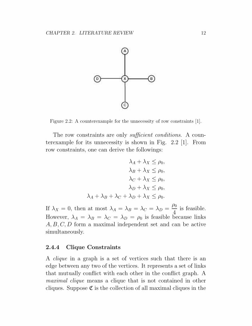
Figure 2.2: A counterexample for the unnecessity of row constraints [1].
The row constraints are only sufficient conditions. A coun-
terexample for its unnecessity is shown in Fig. 2.2 [1]. Fromrow constraints, one can derive the followings:
λA + λX ≤ ρ0,
λB + λX ≤ ρ0,
λC + λX ≤ ρ0,
λD + λX ≤ ρ0,
λA + λB + λC + λD + λX ≤ ρ0.
If λX = 0, then at most λA = λB = λC = λD =ρ0
4is feasible.
However, λA = λB = λC = λD = ρ0 is feasible because linksA,B,C,D form a maximal independent set and can be active
simultaneously.
2.4.4 Clique Constraints
A clique in a graph is a set of vertices such that there is anedge between any two of the vertices. It represents a set of links
that mutually conflict with each other in the conflict graph. Amaximal clique means a clique that is not contained in other
cliques. Suppose C is the collection of all maximal cliques in the

CHAPTER 2. LITERATURE REVIEW 13
conflict graph. Let c ∈ C be any maximal clique. The cliqueconstraints state that:
∑
lu,v∈cλu,v ≤ ρ0, ∀c ∈ C (2.15)
(2.15) forms the clique polytope. (2.15) specifies that the sum
of the traffic carried by the links belonging to the same cliqueshould not exceed the capacity.
The clique constraints are only necessary conditions. A coun-terexample for its insufficiency is shown in Fig. 2.3 [1]. Fromclique constraints, we can derive the followings:
λA + λB ≤ ρ0,
λB + λC ≤ ρ0,
λC + λD ≤ ρ0,
λD + λE ≤ ρ0,
λE + λA ≤ ρ0,
which means λA = λB = λC = λD = λE =ρ0
2is feasible.
However, at most λA = λB = λC = λD = λE =2ρ0
5is feasible
because at most two links can be active at the same time.
2.4.5 Using the physical model
Here we review the extension of the capacity-finding problem tothe physical model. We make use of a weighted conflict graphto reflect the effect on the SNR induced by the amount of inter-
ference received, by assigning the following weight to (lu′,v′, lu,v),where u, v, u′, v′ are all distinct, in the conflict graph [5]:
w(lu′,v′, lu,v) =Pu′,v
Pu,v
γ0
−Nv
(2.16)
In (2.16), Pu,v denotes the power received at node v as a result of
a transmission from node u, and Nv represents the background

CHAPTER 2. LITERATURE REVIEW 14
Figure 2.3: A counterexample for the insufficiency of clique constraints [1].
noise power at node v. In case u, v, u′, v′ are not all distinct, welet w(lu′,v′, lu,v) = ∞ to represent that links (u, v) and (u′, v′)cannot be active simultaneously. As suggested by the formula,
the amount of interference caused by an interfering link dependson the position of the transmitter, so two vertices lu,v and lv,u
should be used in the conflict graph to represent the links be-tween nodes u and v in opposite directions.
We define a counterpart of independent set, called schedulableset, which means a set s such that the following constraint is
satisfied:∑
lu′,v′∈s:(lu′,v′ ,lu,v)∈EF
w(lu′,v′, lu,v) ≤ 1, ∀lu,v ∈ s (2.17)
(2.17) means that for any link in a schedulable set, the cumu-lative interference of other links in the schedulable set should
be small enough so that the resultant SNR is well-above thethreshold γ0, implying that all links in the schedulable set canbe active simultaneously. We also define a maximal schedula-
ble set, which means that addition of any links to this set willviolate (2.17).
Suppose S is the collection of all maximal schedulable sets in

CHAPTER 2. LITERATURE REVIEW 15
the conflict graph. Let s be any maximal schedulable set and fsbe the fraction of time that all links in s can be active simulta-
neously. The schedulable sets impose the following constraints:∑
s∈Sfs ≤ 1 (2.18)
λu,v ≤ ρ0
∑
s : lu,v∈sfs, ∀lu,v ∈ VF (2.19)
(2.18) means that at most only one maximal schedulable set can
be active at a particular time. (2.19) indicates that the fractionof time that a link is active should be upper-bounded by thesum of the amount of the time that it is allowed to be active.
The schedulable set constraints are necessary and sufficient con-ditions for the flows to be schedulable.
2.5 Considering Interference in the Capacity-
Finding Problem with Random Access
To find the capacity of wireless mesh networks with randomaccess protocols, first we need to characterize the stability re-gion of this type of networks. After solving the capacity-finding
problem augmented with the stability region, we get the load-ings on each link. We just need to allocate the amount of flows
on each link according to the results from the capacity-findingproblem and we can achieve the capacity. However, there is lit-
tle work on relating the capacity of a wireless random accessnetwork to the stability region of such a network. Therefore, we
only provide a brief review on the study of the stability regionof wireless networks with slotted ALOHA, the simplest randomaccess protocol.
Almost all works assumed the collision channel model, i.e.,any transmission in the network is successful if and only if there

CHAPTER 2. LITERATURE REVIEW 16
is one active transmitter. This assumption is true only when allstations in the network are sufficiently close to each other.
The study of the stability region ofM -link infinite-buffer slot-ted ALOHA was initiated by [11] decades before, and is still an
ongoing research. The authors in [11] obtained the exact stabil-ity region when M = 2 under collision channel. [2] and [12] usedstochastic dominance and derived the same result as in [11] for
the case of M = 2.For generalM , there were attempts to find the exact stability
region, but there was only limited success. [14] established theboundary of the stability region, but it involves stationary joint
queue statistics, which still do not have closed form to date.Instead of finding the boundary, many researchers focused
on finding bounds on the stability region for general M . [11]obtained separate sufficient and necessary conditions for stabil-ity. [2] and [12] derived tighter bounds on the stability region
by using stochastic dominance in different ways. [3] introducedinstability rank and used it to improve the bounds on the sta-
bility region. However, the bounds in [2] and [3] are not alwaysapplicable. Also, the bounds obtained may not be piecewise
linear.With the advances in multi-user detection, researchers also
studied this stability problem with the multipacket reception
(MPR) model. [15] studied this problem in the infinite-link,single-buffer and symmetric MPR case. [10] considered the prob-
lem with finite links and infinite buffer. They obtained theboundary for the asymmetric MPR case with two links, and
also the inner bound on the stability region for general M .

CHAPTER 2. LITERATURE REVIEW 17
2.6 Chapter Summary
In this Chapter, we have reviewed the capacity-finding prob-lem in wireless mesh networks. We have also introduced vari-
ous ways to incorporate the effects of inter-link interference intothe capacity-finding problem. For wireless mesh networks un-der perfect scheduling, we have the independent set constraints,
the row constraints, the clique constraints and the schedulableset constraints. With wireless mesh networks under random
access, we have to characterize the stability region. However,little work has been done in studying the capacity of wireless
mesh networks with random access protocols. Also, there areother shortcomings in modeling interference in a wireless net-work. These shortcomings will be further elaborated in next
Chapter.
2 End of chapter.

Chapter 3
Partial Interference - Basic Idea
3.1 Introduction
In this Chapter, we point out the deficiencies in the models inChapter 2. Motivated by experimental results in previous stud-
ies, we introduce the notion of partial interference in wirelessnetworks, contrasting with binary interference that can be rep-resented by a single threshold. Partial interference takes into
account the SNR at the receivers and the modulation schemeemployed by the network. We illustrate that by considering par-
tial interference, the gain in capacity across unit cut can be ashigh as 67% under scheduling in a modified Manhattan network.
3.2 Deficiencies in Previous Models
The capacity-finding problem together with the effects of inter-link interference listed in Chapter 2 are formulated based on the
assumptions of protocol model and perfect scheduling. How-ever, we comment that these assumptions only help simplify the
capacity-finding problem and may not be valid in reality.
18

CHAPTER 3. PARTIAL INTERFERENCE - BASIC IDEA 19
3.2.1 Multiple Interferers
The constraints based on the protocol model ignore the case
of multiple interferers. Consider the topology as shown in Fig.3.1. Assume the path loss model is pl(d) = Cd−α where d is the
propagation distance, α is the path loss exponent and C is a con-stant. Also assume the effect of background noise is negligible.
In this topology, node v transmits to node u. The transmit-ters, i.e., nodes v, v′, v′′, all transmit with power P and have the
same transmission range R and interference range R′. Suppose
dv,u = R and R′ is defined byPCR−α
PCR′−α= γ0. Let dv′,u = dv′′,u
andPCd−α
v,u
PCd−αv′,u
= 1.5γ0. Therefore, dv′,u = dv′′,u > R′, and from the
protocol model the transmissions from v′ and v′′ do not inter-fere with the transmission from v to u. From the perspective of
the physical model, when either v′ or v′′ is active but not both,the SNR at u is greater than the required threshold γ0, there-
fore the transmission from v to u will be successful. But whenboth v′ and v′′ are active simultaneously, the SNR at u becomesPCd−α
v,u
2PCd−αv′,u
= 0.75γ0, implying that the transmission from v to u
will be unsuccessful. The primary reason for this discrepancy isthat in the protocol model, only two transmitters are considered
each time, and the possibility of multiple interferers is ignored.Therefore, we should use the physical model, which takes theSNR together with the case of multiple interferers into account,
to model the interference in wireless networks.
3.2.2 Non-binary Behavior of Interference
In the protocol model, it is assumed that when there is inter-
ference between two links, it is not possible for both receiversto decode the signals from the corresponding transmitters when

CHAPTER 3. PARTIAL INTERFERENCE - BASIC IDEA 20
u
v
v’ v’’
Figure 3.1: Protocol model ignores the case of multiple interferers.
both transmitters are active at the same time. This implies when
interference exists between two links, each link can only achievehalf of the capacity if the links share the wireless medium ex-
clusively, or the links can hardly realize any throughput if theyalways attempt transmissions. In both cases, the relationshipbetween the throughput of each link and the separation between
the links can be modeled as a step function. We can obtain sim-ilar relationship from the physical model, in which the abrupt
change is induced by the SNR threshold instead of the thresholddistance, i.e., the interference range.
However, such an abrupt change does not appear in real-ity. In [7], the authors measured the interference among linksin a single-channel, static 802.11 multi-hop wireless network.
They measured the interference between pairs of links by thelink interference ratio, and observed that this ratio exhibited a
continuum between 0 and 1. In [8], two interfering links wereset up in a wireless network with multiple partially overlapped
channels to measure TCP and UDP throughputs of an individ-ual link. It was found that the throughputs increased smoothly
when the separation between the links increased. The through-puts increased more rapidly as the channel separation betweenthe links increased. These experimental results suggest that the
threshold-based or binary assumption in the protocol and thephysical models may not be valid.

CHAPTER 3. PARTIAL INTERFERENCE - BASIC IDEA 21
3.2.3 Impractical Perfect Scheduling
When we include the independent set polytope or clique poly-
tope in the capacity-finding problem, we make an assumptionthat the underlying wireless network operates in a time-division
manner with perfect scheduling. After getting the proportionof time that each link in a wireless network should be active,
time slot assignment algorithms are designed to schedule whenthe links should be active. This requires a centralized scheduler
to coordinate and control the access to the wireless medium bythe links. However, such a perfect scheduling is hard to achievein reality. Moreover, practical wireless networks pre-dominantly
use distributed random access protocols. Therefore, we studythe capacity-finding problem in random access networks.
3.3 Refining the Relationship between Inter-
ference and Throughput Degradation
There have been some preliminary works on finding the relation-ship between the SNR attained at a receiver and the throughputachieved by the corresponding wireless link. In [16], a methodol-
ogy for estimating the packet error rate in the affected wirelessnetwork due to the interference from the interfering wireless
network was presented. The throughput of the affected wirelessnetwork was found to increase continuously with the SNR at-
tained at the corresponding receiver, which increased with theseparation between the networks.
As an illustration to the methodology in [16], assume theunderlying modulation scheme used is binary phase shift keying(BPSK). The distance between the transmitter and the receiver
and that between the interferer and the receiver are dS and dI
meters respectively. The transmission power of the transmitter
and the interferer are PS and PI watts respectively.

CHAPTER 3. PARTIAL INTERFERENCE - BASIC IDEA 22
Assuming the interfering signal can be modeled as additivewhite Gaussian noise (AWGN) and the background noise can be
ignored. We use the two-ray ground reflection model
pl(d) =GTGRh
2Th
2R
d4=C
d4(3.1)
to represent the path loss, where GT and GR are the gain of
transmitter and receiver antenna respectively, hT and hR arethe height of transmitter and receiver antenna respectively, and
C = GTGRh2Th
2R. The path loss exponent is 4 in this model. We
let GT = GR = 1 and hT = hR = 1.5. Then the bit error rate
is1
2erfc(
√γ) [17], where γ is the SNR attained at the receiver
and is equal toPSpl(dS)
PIpl(dI). Suppose all packets consist of L bits.
Then the normalized throughput ρ as a result of the interference
is calculated as follows, assuming both the transmitter and theinterferer are always active:
ρ =
[
1− 1
2erfc(
√γ)
]L
.
We call this partial interference, stating that the result of awireless transmission to be probabilistic based on the corre-sponding signal-to-noise ratio (SNR) and the modulation scheme
used. Fig. 3.2 shows a plot of throughput against distance be-tween the interferer and the receiver in partial interference for
PS = PI = 25 dBm, dS = 300 meters, dI ranging from 400 to700 meters and L = 12000 bits.
In Fig. 3.2 we also plot the variation of throughput againstdistance between the interferer and the receiver if the physical
model is used. The SNR threshold γ0 is calculated by assumingthat when γ = γ0, the packet error rate is 10−3, i.e.,
10−3 = 1−[
1− 1
2erfc(
√γ0)
]L
.

CHAPTER 3. PARTIAL INTERFERENCE - BASIC IDEA 23
400 450 500 550 600 650 7000
0.2
0.4
0.6
0.8
1
Network Separation (m)N
orm
aliz
ed T
hrou
ghpu
t
Relationship between Throughput and Network Separation
BinaryPartial
Figure 3.2: Throughput degradation and network separation.
We observe that if the value we assign to γ0 is too large (or thethreshold distance is too large), we underestimate the through-
put that the links can achieve. On the other hand, if γ0 istoo small (or the threshold distance is too small), we introduce
excessive interference into the network. In other words, it isdifficult to use a single threshold to describe accurately the re-
lationship between interference and throughput of each link ina network.
3.4 Capacity Gain by Exploiting Partial In-
terference
In this Section, we demonstrate that there is a gain in capacity
by exploiting partial interference. We consider one variationof the Manhattan network [18], i.e., a network consisting of a
rectangular grid extending to infinity in both dimensions. Thehorizontal and vertical separation between neighboring stations
are denoted by r and d respectively. The capacity of each linkwithout interference is denoted by ρ0.
We assume differential binary phase shift keying (DBPSK) is
employed and a packet consists of L bits. We use the two-rayground reflection model (3.1) as in previous Section to model
the path loss. To apply the physical model, we let the SNR

CHAPTER 3. PARTIAL INTERFERENCE - BASIC IDEA 24
−6 −4 −2 0 2 4 6−6
−4
−2
0
2
4
6A Sample Schedule
Figure 3.3: A scheduling pattern in the modified Manhattan network.
threshold γ0 be the case that the packet error rate is ε, i.e.,
1−[
1− 1
2exp(−γ0)
]L
= ε, where1
2exp(−γ) is the bit error rate
of DBPSK [17]. We let L = 8192 and ε = 10−3, therefore the
SNR requirement is γ0 = 15.23. Assuming there is no interferer,this SNR requirement is met when the length of a link is smaller
than 493 meters.We use a Cartesian coordinate plane to represent the modified
Manhattan network. One station is placed at every point withintegral coordinates in the network. Suppose we schedule flowsin the modified Manhattan network from the South to the North
using the pattern shown in Fig. 3.3 and its shifted versions. InFig. 3.3, an arrow is used to represent an active link, where the
tail and the head of an arrow denote the transmitter and thereceiver of the link respectively.
We use the capacity across unit cut η(µ) as the performance
metric, where µ =r
dis the ratio of the horizontal separation
to the vertical separation. It is a measure on how much we
can send through a cut on average while packing the links to-gether. Consider the SNR attained at the receiver marked with
the blue circle, which has the position assigned as the origin inthe Cartesian coordinate plane. We assume all stations transmit
with power P , and each station has a background noise power

CHAPTER 3. PARTIAL INTERFERENCE - BASIC IDEA 25
of N . The SNR is defined by γ(µ) =S
N + I(µ), where S is
the received power from the intended transmitter and I(µ) isthe power received from all interferers. The capacity achieved
by each link is ρ(µ) = ρ0
1 − 1
2exp[−γ(µ)]
L
under partial
interference; while in the physical model, we let ρ(µ) = ρ0 if
γ(µ) ≥ γ0 and ρ(µ) = 0 otherwise. A cut C in the network isan infinitely long horizontal line. Let Tnn∈N be the set of allactive transmitters such that C intersects the link used by Tn.
We divide C into segments C(Tn), n ∈ N, where
C(Tn) =
x ∈ C : ‖x− Tn‖ = minn′∈N‖x− Tn′‖
and ‖·‖ is the Euclidean norm. Then the length L of the cut
occupied by an active transmitter is the length of C(Tn), and
the capacity across unit cut is therefore η(µ) =fρ(µ)
L , where f
is the fraction of time that a link is active.In the following we assume d = 450 meters, P = 24.5 dBm
and N = −88 dBm. For the schedule in Fig. 3.3, the signal
power is S =PC
d4. All transmitters in Fig. 3.3 are located at
positions (x, 4y−1), where x and y are integers. The interference
power is
I(µ) =
∞∑
x=−∞
∞∑
y=−∞
PC(
(xr)2 + [(4y − 1)d]2)2 −
PC
d4
=
∞∑
x=−∞
∞∑
y=−∞[(xµ)2 + (4y − 1)2]−2 − 1
PC
d4.
Considering the physical model, if the schedule is allowed to
be active, we need µ ≥ µ0 = 5.58, as listed in Table 3.1 anddepicted in Fig. 3.4 by the blue dashed line. The value of µ0
is obtained from γ(µ0) = γ0. Each active transmitter occupies

CHAPTER 3. PARTIAL INTERFERENCE - BASIC IDEA 26
2 3 4 5 6 7 80
0.05
0.1
0.15
0.2
0.25
Capacity across Unit Cut against Separation Ratio
Ratio of Horizontal to Vertical SeparationN
orm
aliz
ed C
apac
ity a
cros
s U
nit C
ut (
km−
1 )
dist=350m partialdist=350m binarydist=400m partialdist=400m binarydist=450m partialdist=450m binary
Figure 3.4: Capacity across unit cut for different length of links under thephysical model (binary interference) and partial interference.
Table 3.1: Capacity gain in the modified Manhattan network with differentlength of links.
d µ0 η(µ0) µopt η(µopt) % increase
350 3.02 0.2365 ρ0 2.55 0.2671 ρ0 12.93%
400 3.48 0.1796 ρ0 2.73 0.2163 ρ0 20.45%
450 5.58 0.0996 ρ0 3.06 0.1661 ρ0 66.82%
a cut of length r = µd and each link is active for one quarter
of a cycle. Therefore, for µ = µ0, the maximum capacity across
unit cut under the physical model isρ0
4µ0d= 0.0996ρ0 bits per
second per kilometer.
If we allow partial interference, the active transmitters canbe packed more closely. When µ decreases, more spatial reuse
is allowed. The increase in the density of active transmittersoutweighs the degradation in capacity, so there is an increase in
the capacity across unit cut. However, if µ decreases further,interference will be the dominant factor in determining the ca-pacity across unit cut. Therefore, the capacity across unit cut
drops, and there exists µopt for the optimal performance underpartial interference. This behavior is depicted by the blue solid
line in Fig. 3.4. The optimal value of µ under partial interfer-ence is µopt = 3.06, and the capacity across unit cut is 0.1661ρ0

CHAPTER 3. PARTIAL INTERFERENCE - BASIC IDEA 27
bits per second per kilometer. There is a percentage increaseof 66.82% in the capacity across unit cut by exploiting partial
interference. Similar results are shown in Table 3.1 and Fig.3.4 for d = 350, 400 meters. The percentage increase is larger
when the links are longer, but the capacity achieved by eachlink reduces. We can view µ0d as the carrier sensing range inthe modified Manhattan network with the scheduling pattern in
Fig. 3.3, as it is the smallest horizontal separation allowed bythe physical model. We observe that if the length of the links
increases, the carrier sensing range needs to be increased in alarger proportion. Also, this carrier sensing range is much larger
than double of the length of the links, which is the usual con-vention used in defining the relationship between carrier sensing
range and transmission range.

CHAPTER 3. PARTIAL INTERFERENCE - BASIC IDEA 28
3.5 Chapter Summary
In this Chapter, we have reviewed the deficiencies in the modelsin previous Chapter. We also introduced the notion of partial in-
terference in wireless networks, and illustrated that by exploitingpartial interference in scheduling in a regular wireless network,the performance gain in terms of capacity across unit cut can
be as high as 67%. The example included here only consideredpartial interference in wireless networks with perfect scheduling.
In the next two Chapters, we will study partial interference inwireless networks with random access protocols, i.e., 802.11 and
slotted ALOHA. Performance gain in terms of capacity by ex-ploiting partial interference in random access networks will bedemonstrated.
2 End of chapter.
Chapter 4
Partial Interference in 802.11
4.1 Introduction
In this Chapter, we study partial interference in 802.11 networks,the prevalent wireless random access networks. We present an
analytical framework to characterize partial interference in asingle-channel wireless network under unsaturated traffic condi-tions, which uses 802.11b with basic access scheme and DBPSK.
We show that there is a partial interference region, in which thethroughput of each link increases continuously with the sepa-
ration between the links in the network. An analogy is drawnbetween partial interference and code division multiple access to
demonstrate their similarities. As a first attempt to relate thecapacity-finding problem in wireless random access networks tothe stability region of such networks, we derive the admissible
(stability) region of an 802.11 network with two links numeri-cally.
4.2 The 802.11 Model
We present our framework to characterize partial interferencein a wireless network with random access protocols. In this
framework, we derive the transmission probabilities τn and the
29

CHAPTER 4. PARTIAL INTERFERENCE IN 802.11 30
packet corruption probabilities cn of the links in the network. τnis the probability that a station transmits in a randomly chosen
slot, while cn is the probability that a packet is received witherror.
4.2.1 Assumptions
For illustration, we choose the MAC and PHY protocols tobe 802.11b with basic access scheme and 1Mbps DBPSK. Ourmodel can be readily extended to consider other modulation
schemes. In addition, we make the following assumptions:
• The network consists of two links (T1, R1) and (T2, R2),where Tn and Rn denote the transmitter and the receiver
of the links respectively, n = 1, 2.• There are a constant buffer nonempty probability qn that
the transmission buffer of Tn is nonempty and a constantchannel idle probability in that Tn senses the channel to be
idle, n = 1, 2.• Tn transmits with power Pn, and the background noise
power at Rn is Nn, n = 1, 2.
• Channel defects like shadowing and fading are neglected,and a generic path loss model pl(d) = Cd−α is used to
model the wireless channel, where d is the propagation dis-tance, α is the path loss exponent and C is a constant.
• The interference from other transmitters plus the receiverbackground noise is assumed to be Gaussian distributed.• All bits in a packet must be received correctly for correct
reception of the packet.• The size of an acknowledgement is much smaller than that
of the payload, so the bit errors on acknowledgement arenegligible.

CHAPTER 4. PARTIAL INTERFERENCE IN 802.11 31
4.2.2 Transmission Probability Calculation
We follow the approach as in [9], using a discrete-time Markov
chain to model the 802.11 Distributed Coordination Function(DCF) and obtain the transmission probability of a station. An
ordered pair (j, k) is used to denote the state of the Markovchain, where j represents the backoff stage, and k is the current
backoff counter value. In stage j, k is in the range [0,Wj − 1],where Wj is the contention window size in stage j. m is the
maximum number of backoff stages. However, there are somediscrepancies between this model and the actual behavior of802.11 DCF. First, the model assumes that a station retransmits
indefinitely until the packet is successfully transmitted. This as-sumption is inconsistent with 802.11 basic access scheme. Also,
the model does not account for the unsaturated traffic condi-tions, which is the scenario appeared in practical situations.
We adopt the following modifications on the Markov chain toobtain a better model. First, we take into account the limitednumber of retransmissions in 802.11 as in [19], by restricting the
Markov chain to leave the m-th backoff stage once the stationtransmits a packet in that backoff stage. Second, we follow [19]
to modify the values of Wj in accordance with the 802.11 MACand PHY specifications [20], with m′ corresponding to the first
backoff stage using the maximum contention window size:
Wj =
2jW0, 0 ≤ j ≤ m′
2m′
W0, m′ < j ≤ m.
In addition, to model the unsaturated conditions, we follow
[21] to augment the Markov chain by introducing new states(−1, k), k ∈ [0,W0 − 1]. These new states represent the statesof being in the post-backoff stage. The post-backoff stage is en-
tered whenever the station has no packets queued in its transmis-sion buffer after a successful transmission. The corresponding
Markov chain is depicted in Fig. 4.1.

CHAPTER 4. PARTIAL INTERFERENCE IN 802.11 32
−1,W0−1−1,1−1,0
0,W0−10,10,0
1,W1−11,11,0
j,Wj−1j,1j,0
m,Wm
−1m,1m,0
......
......
......
......
......
......
......
...... ...... ......
...... ...... ......
Figure 4.1: A Markov chain model for 802.11 DCF in unsaturated conditions.
We use Pr(j1, k1|j0, k0) to denote the transition probability
from (j0, k0) to (j1, k1), and the transition probabilities are asfollows:
Pr(j, k|j, k + 1) = 1,
j ∈ [0, m], k ∈ [0,Wj − 2], (4.1)
Pr(0, k| − 1, k + 1) = qn, k ∈ [0,W0 − 2], (4.2)
Pr(−1, k| − 1, k + 1) = 1− qn, k ∈ [0,W0 − 2], (4.3)
Pr(0, k|j, 0) =(1− cn)qn
W0,
j ∈ [0, m− 1], k ∈ [0,W0 − 1], (4.4)
Pr(−1, k|j, 0) =(1− cn)(1− qn)
W0,
j ∈ [0, m− 1], k ∈ [0,W0 − 1], (4.5)

CHAPTER 4. PARTIAL INTERFERENCE IN 802.11 33
Pr(0, k|m, 0) =qnW0
, k ∈ [0,W0 − 1], (4.6)
Pr(−1, k|m, 0) =1− qnW0
, k ∈ [0,W0 − 1], (4.7)
Pr(j, k|j − 1, 0) =cnWj
,
j ∈ [1, m], k ∈ [0,Wj − 1], (4.8)
Pr(0, k| − 1, 0) =qn(1− in) + q2
nin(1− cn)W0
,
k ∈ [0,W0 − 1], (4.9)
Pr(1, k| − 1, 0) =qnincnW1
, k ∈ [0,W1 − 1], (4.10)
Pr(−1, k| − 1, 0) =qnin(1− cn)(1− qn)
W0,
k ∈ [1,W0 − 1], (4.11)
Pr(−1, 0| − 1, 0) =qnin(1− cn)(1− qn)
W0+ (1− qn). (4.12)
The equations above describe the following behaviors:
• the decrement of backoff counter at the beginning of eachslot by (4.1)-(4.3);
• the reset of backoff procedure to stage 0 or -1 after a suc-cessful transmission by (4.4)-(4.5);• the reset of backoff procedure to stage 0 or -1 after the last
transmission attempt by (4.6)-(4.7);• the increment of backoff stage after an unsuccessful trans-
mission by (4.8);• the transition after post-backoff finishes by (4.9)-(4.12).
Let πj,k denote the stationary probability of the state (j, k) in
the Markov chain. The transmission probability of a station is

CHAPTER 4. PARTIAL INTERFERENCE IN 802.11 34
given by
τn = π−1,0qnin +
m∑
j=0
πj,0
=
(
2q2nW0
m∑
j=0
cjn
)
q2nW0
m∑
j=0
cjn(Wj + 1)
+ (1− qn)[
1− (1− qn)W0
]
× [qn(1− in)(W0 + 1) + 2(1− qn)]−1
. (4.13)
The derivation of this equation is given in Appendix.
4.2.3 Packet Corruption Probability Calculation
The packet corruption probability is calculated according to the
modulation scheme used in the PHY layer, the distance betweenthe transmitter and the receiver, and the existence of nearby
interferer(s). For a fixed carrier sensing threshold β, we differ-entiate into two cases, whether both transmitters can sense the
transmission of each other or not.If T1 can sense the transmission of T2, i.e., P2pl
(
dT1,T2
)
> β,
where dX,Y is the distance between X and Y , then the SNR atR1 is
γ1 =P1pl
(
dT1,R1
)
N1.
The bit error rate attained by (T1, R1) is e(γ1) =1
2exp(−γ1),
and the packet corruption probability for (T1, R1) is
c1 = 1− [1− e(γ1)]HP+HM+L, (4.14)
where HP , HM and L represent the number of bits in the PHYheader, the MAC header and the payload respectively.
CHAPTER 4. PARTIAL INTERFERENCE IN 802.11 35
On the other hand, if T1 cannot sense the transmission of T2,i.e., P2pl
(
dT1,T2
)
≤ β, then the SNR at R1 depends on whether
T2 is active in transmission or not, i.e.,
Prγ1 = γ =
1− τ2, γ =P1pl
(
dT1,R1
)
N1
τ2, γ =P1pl
(
dT1,R1
)
N1 + P2pl(
dT2,R1
)
.
The packet corruption probability is calculated by the average
bit error rate E[e(γ1)]:
c1 = 1−(
1−E[e(γ1)])HP +HM+L
. (4.15)
The channel idle probability is defined as follows. If T1 cansense the transmission of T2, then T1 will consider the channel
to be idle whenever T2 is inactive, i.e., i1 = 1− τ2; otherwise T1
always senses the channel to be idle and i1 = 1.
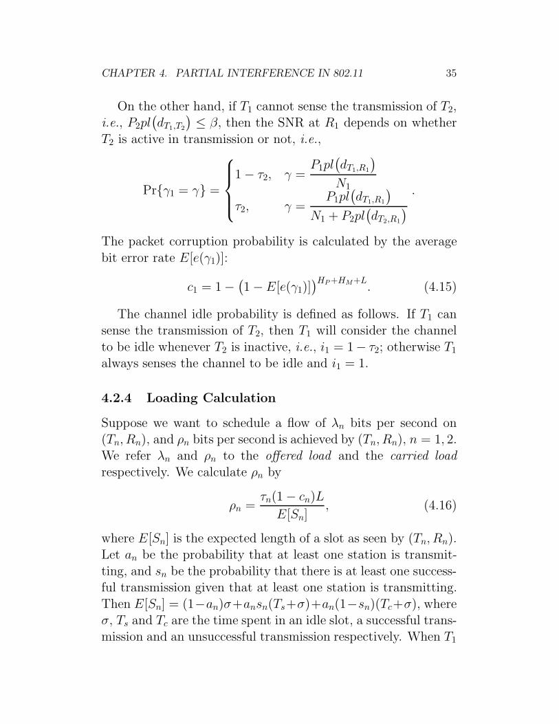
4.2.4 Loading Calculation
Suppose we want to schedule a flow of λn bits per second on(Tn, Rn), and ρn bits per second is achieved by (Tn, Rn), n = 1, 2.We refer λn and ρn to the offered load and the carried load
respectively. We calculate ρn by
ρn =τn(1− cn)LE[Sn]
, (4.16)
where E[Sn] is the expected length of a slot as seen by (Tn, Rn).Let an be the probability that at least one station is transmit-
ting, and sn be the probability that there is at least one success-ful transmission given that at least one station is transmitting.
Then E[Sn] = (1−an)σ+ansn(Ts+σ)+an(1−sn)(Tc+σ), whereσ, Ts and Tc are the time spent in an idle slot, a successful trans-mission and an unsuccessful transmission respectively. When T1

CHAPTER 4. PARTIAL INTERFERENCE IN 802.11 36
can sense the transmission of T2, we consider both links to beone system:
a1 = 1− (1− τ1)(1− τ2),s1 =
1− [1− τ1(1− c1)][1− τ2(1− c2)]a1
.
Otherwise, we treat both links to be separate systems:
a1 = τ1,
s1 = 1− c1.
We approximate the packet arrival of (Tn, Rn) to be a Poisson
process with rateλn
L, n = 1, 2, and estimate the buffer nonempty
probability by
qn = 1− exp
−λn
LE[Sn]
. (4.17)
4.2.5 Summary
In summary, if T1 can sense the transmission of T2, then we
obtain the following set of equations for (T1, R1):
τ1 =
(
2q21W0
m∑
j=0
cj1
)
q21W0
m∑
j=0
cj1(Wj + 1)
+ (1− q1)[
1− (1− q1)W0
]
× [q1τ2(W0 + 1) + 2(1− q1)]−1
,
c1 = 1− [1− e(γ1)]HP +HM+L,
q1 = 1− exp
−[(
1− [1− τ1(1− c1)][1− τ2(1− c2)])
Ts
+ [τ1c1 + τ2c2 − τ1τ2(c1 + c2 − c1c2)]Tc + σ]λ1
L
.

CHAPTER 4. PARTIAL INTERFERENCE IN 802.11 37
Otherwise, we obtain another set of equations for (T1, R1):
τ1 =
(
2q21W0
m∑
j=0
cj1
)
q21W0
m∑
j=0
cj1(Wj + 1)
+ 2(1− q1)2[
1− (1− q1)W0
]
−1
,
c1 = 1−(
1− E[e(γ1)])HP +HM+L
,
q1 = 1− exp
−[τ1(1− c1)Ts + τ1c1Tc + σ]λ1
L
.
Similarly, we can obtain three equations for link (T2, R2). Withthese six equations we can solve for the variables τ1, c1, q1, τ2, c2, q2by Newton’s method [22], and obtain the loadings of these two
links by (4.16).
4.3 Some Analytical Results
We use the two-ray ground reflection model
pl(d) =GTGRh
2Th
2R
d4=C
d4
to represent the path loss as in Chapter 3 and the values in Table4.1 to obtain numerical results from our model. These values
are defined in or derived from the values in the 802.11 MAC andPHY specifications [20] or NS-2 [23].
In the following we attempt to find the maximum carriedloads of each link in various scenarios. One observation from
solving the system of equations in Section 4.2 is that the carriedload will be smaller than the offered load when the offered load istoo large. This corresponds to the instability of 802.11 observed
in previous works (e.g., [9]). Therefore, we use binary search tofind the maximum carried load under stable conditions. Initially,
the search range for the offered load is between 0 and 1Mbps. We

CHAPTER 4. PARTIAL INTERFERENCE IN 802.11 38
Table 4.1: Parameters used for the analytical results of 802.11.
HP 192 bits HM 272 bits m 7 m′ 5
Ts 9020 µs Tc 9020 µs σ 20 µs W0 32
P1, P2 24.5 dBm N1, N2 -88 dBm Gt, Gr 1 ht, hr 1.5 m
T1
R1
T2
R2
Figure 4.2: A sample topology.
choose the midpoint of the search range to be the offered loadand solve the system of equations. If the resultant carried load
is the same as the offered load, the offered load can be increasedand the next search range will be the upper half of the original
one. Otherwise, the offered load results in instability and thenext search range will be the lower half of the original one. This
procedure is repeated until the search range is sufficiently small.We consider a network of two parallel links as shown in Fig.
4.2, with d and r representing the length of the links and the
link separation respectively. The link separation is defined asthe perpendicular distance between the links. We let L = 8192
bits, d = 450 meters, and β = −70,−75,−78,−80 dBm to solvefor the maximum carried loads and obtain the curves as shown
in Figs. 4.3(a)-4.3(d).Consider the curve corresponding to the carrier sensing thresh-
old of -78 dBm in Fig. 4.3(c), which is a common value used inNS-2 simulation and the practical value used in Orinoco wire-less LAN card. The corresponding carrier sensing range is 550
meters, which is in line with the carrier sensing range used inpractice. In our model, we assume that carrier sensing works
when the separation is within the carrier sensing range and failsotherwise, and use two different sets of equations to model the

CHAPTER 4. PARTIAL INTERFERENCE IN 802.11 39
system in these situations. Therefore there is an abrupt changein the aggregate throughput when the separation equals the car-
rier sensing range. If there is no carrier sensing in the system,the aggregate throughput will reduce to zero smoothly when the
link separation reduces.The curve in Fig. 4.3(c) can be divided into three parts ac-
cording to the link separation r. When r < 550 meters, both
transmitters are in the carrier sensing range of each other. Asa result, at most only one transmitter is active at a time. If
r ≥ 550 meters, the transmitters are unaware of the existence ofeach other, and they contend for the wireless channel as if there
were no interferers nearby. When r > 800 meters, the separa-tion is so large that there will not be any interference between
the links. When r lies between 550 and 800 meters, the aggre-gate throughput of the links increases smoothly as r increases.We label this range of r as the partial interference region. The
existence of this partial interference region suggests that the in-terference models proposed by [4] that a single threshold can
represent the interference relationship in wireless networks maybe overly simplified.
The width of this partial interference region depends on thecarrier sensing threshold β used. Smaller β, e.g., -80 dBm, re-sults in a narrower partial interference region as in Fig. 4.3(d).
Simultaneous transmissions are allowed only for the links sepa-rated far enough, and the throughput is suppressed significantly.
For larger β, e.g., -75 and -70 dBm, more spatial reuse is al-lowed, and the width of the partial interference region is larger,
as shown in Figs. 4.3(a)-4.3(b). However, excessive interferenceis introduced for larger β, so there is a reduction in the aggregate
throughput.Besides carrier sensing threshold, the length of the links d also
affects the partial interference region. We reduce d to be 400
meters, and obtain the results in Figs. 4.4(a)-4.4(d). As shown

CHAPTER 4. PARTIAL INTERFERENCE IN 802.11 40
300 400 500 600 700 800 9000
0.5
1
1.5
2Aggregate Throughput against Link Separation
Distance between T1 and T
2 (m)
Agg
rega
te T
hrou
ghpu
t (M
bps)
CST=−70dBm
(a) -70 dBm.
300 400 500 600 700 800 9000
0.5
1
1.5
2Aggregate Throughput against Link Separation
Distance between T1 and T
2 (m)
Agg
rega
te T
hrou
ghpu
t (M
bps)
CST=−75dBm
(b) -75 dBm.
300 400 500 600 700 800 9000
0.5
1
1.5
2Aggregate Throughput against Link Separation
Distance between T1 and T
2 (m)
Agg
rega
te T
hrou
ghpu
t (M
bps)
CST=−78dBm
(c) -78 dBm.
300 400 500 600 700 800 9000
0.5
1
1.5
2Aggregate Throughput against Link Separation
Distance between T1 and T
2 (m)
Agg
rega
te T
hrou
ghpu
t (M
bps)
CST=−80dBm
(d) -80 dBm.
Figure 4.3: Aggregate throughput for the topology in Fig. 4.2 with lengthof links = 450 meters and various carrier sensing thresholds.
in Figs. 4.4(a)-4.4(d), the partial interference region becomesnarrower for all values of carrier sensing threshold. Also, theaggregate throughput achieved by the links is larger for the same
link separation when the links are shortened.
4.4 A TDMA/CDMA Analogy
In this Section, we use TDMA, CDMA and Shannon’s capac-
ity to establish an analogy to our results in previous Section.Consider the same network as in Fig. 4.2. The bandwidth of
the channel is denoted by B. Both transmitters transmit withpower P and the background noise power at each receiver is N .
If the links use TDMA as the multiplexing scheme to sharethe wireless channel, then only one link can be active at a time.
So there is no interference, and the SNR at the receiver of each

CHAPTER 4. PARTIAL INTERFERENCE IN 802.11 41
300 400 500 600 700 800 9000
0.5
1
1.5
2Aggregate Throughput against Link Separation
Distance between T1 and T
2 (m)
Agg
rega
te T
hrou
ghpu
t (M
bps)
CST=−70dBm
(a) -70 dBm.
300 400 500 600 700 800 9000
0.5
1
1.5
2Aggregate Throughput against Link Separation
Distance between T1 and T
2 (m)
Agg
rega
te T
hrou
ghpu
t (M
bps)
CST=−75dBm
(b) -75 dBm.
300 400 500 600 700 800 9000
0.5
1
1.5
2Aggregate Throughput against Link Separation
Distance between T1 and T
2 (m)
Agg
rega
te T
hrou
ghpu
t (M
bps)
CST=−78dBm
(c) -78 dBm.
300 400 500 600 700 800 9000
0.5
1
1.5
2Aggregate Throughput against Link Separation
Distance between T1 and T
2 (m)
Agg
rega
te T
hrou
ghpu
t (M
bps)
CST=−80dBm
(d) -80 dBm.
Figure 4.4: Aggregate throughput for the topology in Fig. 4.2 with lengthof links = 400 meters and various carrier sensing thresholds.
link is γ =PCd−α
N. Then by Shannon’s capacity formula [17],
the aggregate capacity is
ρTDMA = B log2(1 + γ).
If CDMA is used instead, then the SNR at the receiver of
each link will bePCd−α
N + PC(d2 + r2)−α2
=1
γ−1 + z, where z =
(
d2
d2 + r2
)α2
. The aggregate capacity is
ρCDMA = 2B log2
(
1 +1
γ−1 + z
)
.
Fig. 4.5 shows the variation of aggregate capacity againstlink separation in TDMA and CDMA, normalized by the ca-
pacity in TDMA, with d = 450 meters. The aggregate capacity

CHAPTER 4. PARTIAL INTERFERENCE IN 802.11 42
0 500 1000 1500 2000 2500 30000
0.5
1
1.5
2
Distance between T1 and T
2 (m)
Nor
mal
ized
Agg
rega
te C
apac
ity
TDMA and CDMA
TDMACDMA
Figure 4.5: A TDMA/CDMA analogy for the results in Section 4.3.
is independent of the link separation in TDMA, and increasessmoothly with the link separation in CDMA. There exists acrossover point r0 such that, when r < r0, TDMA has a higher
aggregate capacity, and the opposite occurs otherwise. The no-tion of setting a carrier sensing threshold or range can be viewed
as deciding when to switch between TDMA and CDMA: useTDMA when the separation is smaller than the carrier sensing
range, use CDMA otherwise. Carrier sensing allows at most onelink to be active at a time, so the links within carrier sensingrange share the wireless channel like TDMA. Partial interference
is analogous to CDMA that the aggregate throughput increasessmoothly as the link separation increases. We can obtain the
behavior in previous Section by setting the carrier sensing rangeto be close to r0, and achieve optimal performance in terms of
aggregate capacity by setting the carrier sensing range to be r0.
4.5 Admissible (Stability) Region
As an attempt to obtain the capacity of 802.11 networks under
partial interference, we compute the admissible (stability) regionpredicted from our model. The admissible region includes all
flow vectors (λ1, λ2) such that if (λ1, λ2) is located inside theadmissible region, then a flow of λn can be allocated on and

CHAPTER 4. PARTIAL INTERFERENCE IN 802.11 43
0 0.2 0.4 0.6 0.8 10
0.2
0.4
0.6
0.8
1Admissible Region
Throughput of Link 1 (Mbps)T
hrou
ghpu
t of L
ink
2 (M
bps)
dist=500mdist=600mdist=900m
Figure 4.6: Admissible region for various link separations.
achieved by (Tn, Rn), n = 1, 2. We use the same settings asabove, and choose the carrier sensing threshold to be -78 dBm.
The link separations are chosen to be 500, 600 and 900 metersfor illustrative purposes, because they correspond to different
shapes of the admissible region. Fig. 4.6 shows the admissibleregion for these three link separations. The link separation of
500 meters represents that the links are in mutual interference,and the admissible region has a triangular shape. When the
links are separated by 900 meters, the links do not interferewith each other, and the admissible region is rectangular. Forthe link separation of 600 meters, partial interference exists and
the admissible region becomes convex.Although we are able to compute the admissible region for a
two-link 802.11 network numerically, the closed-form expressionfor the admissible region is unknown. Also, for an 802.11 net-
work with two links, we have to solve a system of six nonlinearequations to compute the admissible region. When the numberof links in the network grows, the number of equations involved
will increase and the system of equations will be more difficultto solve. Therefore the computation of the admissible region of
general 802.11 networks seems to be forbiddingly intractable.

CHAPTER 4. PARTIAL INTERFERENCE IN 802.11 44
4.6 Chapter Summary
In this Chapter, we have introduced an analytical framework tocharacterize partial interference in 802.11 networks. We have
also demonstrated that there is a partial interference region,such that when the separation between the links falls in thisregion, the throughput of each link increases continuously with
the link separation. Also, we have computed numerically thestability region of 802.11 networks with two links under partial
interference. The computation of the stability region in this caseis difficult to generalize when there are more links in the network.
Therefore, in next Chapter, we study the stability region of asimpler random access protocol, i.e., slotted ALOHA.
2 End of chapter.

Chapter 5
Partial Interference in SlottedALOHA
5.1 Introduction
In Chapter 4, we attempted to find the stability region of 802.11networks. When there are two links in the network, we have to
solve a system of nonlinear equations. If more links are addedto the network, the system of nonlinear equations we need tosolve would be increasingly more complicated. Also, the results
obtained in Chapter 4 can only be computed numerically but notanalytically. From these, the stability region of general 802.11
networks seems to be computationally intractable.In order to obtain insights in the stability region of general
802.11 networks, in this Chapter, we study the stability of slot-ted ALOHA, which is a simpler random access protocol, under
the assumptions of finite links and infinite buffer. By consider-ing partial interference, for the case of two links, we computeanalytically the exact stability region. From this, we observe
that there is a gradual transition from the collision channel tothe orthogonal channel when the link separation increases. The
stability region can be either convex or nonconvex, dependingon the link separation and the transmission probability vector.
A partial characterization on the boundary of the stability re-
45

CHAPTER 5. PARTIAL INTERFERENCE IN SLOTTED ALOHA 46
gion in closed form for the case of general number of links is alsogiven.
5.2 The Finite-Link Slotted ALOHA Model
5.2.1 Assumptions
Let M = nMn=1 be the set of links in the slotted ALOHAsystem. Time is slotted. The following assumptions apply toall links n ∈ M. Let Tn and Rn be the transmitter and the
receiver of link n respectively. Tn has an infinite buffer. Thepacket arrival process at Tn is Bernoulli with mean λn and is
independent of the arrivals at other transmitters. Tn attemptsa virtual transmission with probability pn, i.e., if its buffer is
nonempty, Tn attempts an actual transmission with probabilitypn; otherwise, Tn always remains silent. Also define pn = 1−pn.
In the system, each time slot is just enough for transmission
of one packet. Packets are assumed to have equal lengths. Weassume transmission results are independent in each slot. For
n ∈ A ⊆ M, let qMn,A be the probability that the transmis-sion on link n is successful when Tn′n′∈A is the set of active
transmitters. qMn,A depends on the SNR at the receiver and themodulation scheme used. We also assume the transmitters know
immediately the transmission results, so that the transmittersremove successfully transmitted packets and retain only thoseunsuccessful ones.
5.2.2 Stability of Slotted ALOHA
We let Qn(t), t ∈ N be the queue length in Tn at the begin-ning of slot t, and use a M -dimensional Markov chain QM(t) =(
Qn(t))
n∈M to represent the queue lengths in all transmitters.We denote by An(t) the number of packets arrived at Tn in slot t,
and Dn(t) the number of packets successfully transmitted in slot

CHAPTER 5. PARTIAL INTERFERENCE IN SLOTTED ALOHA 47
t by Tn when Qn(t) > 0. Then Qn(t + 1) = [Qn(t)−Dn(t)]+ +
An(t), where [z]+ = max0, z is used to account for the case
that there is no packet transmitted when Qn(t) = 0. We use thedefinition of stability in [3, 10, 14].
Definition 5.1. A M-dimensional stochastic process QM(t) is
stable if for x ∈ NM the following holds:
limt→∞
Pr
QM(t) < x
= F (x) and limx→∞
F (x) = 1.
If the following weaker condition holds instead,
limx→∞
lim inft→∞
Pr
QM(t) < x
= 1,
then the process is substable. The process is unstable if it is
neither stable nor substable.
The stability problem of slotted ALOHA we consider here isto determine whether the slotted ALOHA system with the set oflinks M is stable given the parameters λnn∈M and pnn∈M.
We use the result from [24]: On the assumption that the arrivaland the service processes of a queue are stationary, the queue is
stable if the average arrival rate is less than the average servicerate, and the queue is unstable if the average arrival rate is
larger than the average service rate. We also define the slottedALOHA system to be stable when all queues in the system are
stable.
5.3 Stability Region of 2-Link Slotted ALOHA
under Partial Interference
We extend the model in [10] to obtain the following results. For
n ∈ M, let Pn and Nn be the transmission power used by Tn
and the background noise power at Rn respectively. Assume the
signal propagation follows the path loss model pl(d) = Cd−α,

CHAPTER 5. PARTIAL INTERFERENCE IN SLOTTED ALOHA 48
where d is the propagation distance, α is the path loss exponentand C is a constant. We let γMn,A be the SNR attained at Rn
when Tn′n′∈A is the set of active transmitters. Assume a packetconsists of L bits. Let e(γ) be the bit error rate when the SNR
is γ. In particular, if DBPSK is used in the physical layer,
e(γ) =1
2exp(−γ). Under binary interference, we let the SNR
threshold γ0 be the case that the packet error rate is ε, i.e.,
1−[
1 − 1
2exp(−γ0)
]L
= ε. Consider M = 2. When only T1 is
active, the SNR attained at R1 is γM1,1 =P1Cd
−αT1,R1
N1, and
qM1,1 =
1, γM1,1 ≥ γ0
0, γM1,1 < γ0
, (5.1)
where dX,Y is the distance between X and Y . When both T1
and T2 are active, then γM1,1,2 =P1Cd
−αT1,R1
P2Cd−αT2,R1
+N1is the SNR
attained at R1, and
qM1,1,2 =
1, γM1,1,2 ≥ γ0
0, γM1,1,2 < γ0
. (5.2)
If we consider partial interference instead, we can calculate qMn,Aas follows. When only T1 is active,
qM1,1 =[
1− e(
γM1,1
)]L
. (5.3)
When both T1 and T2 are active,
qM1,1,2 =[
1− e(
γM1,1,2
)]L
. (5.4)
Similarly, we can derive expressions for qM2,2 and qM2,1,2 under
binary and partial interference.
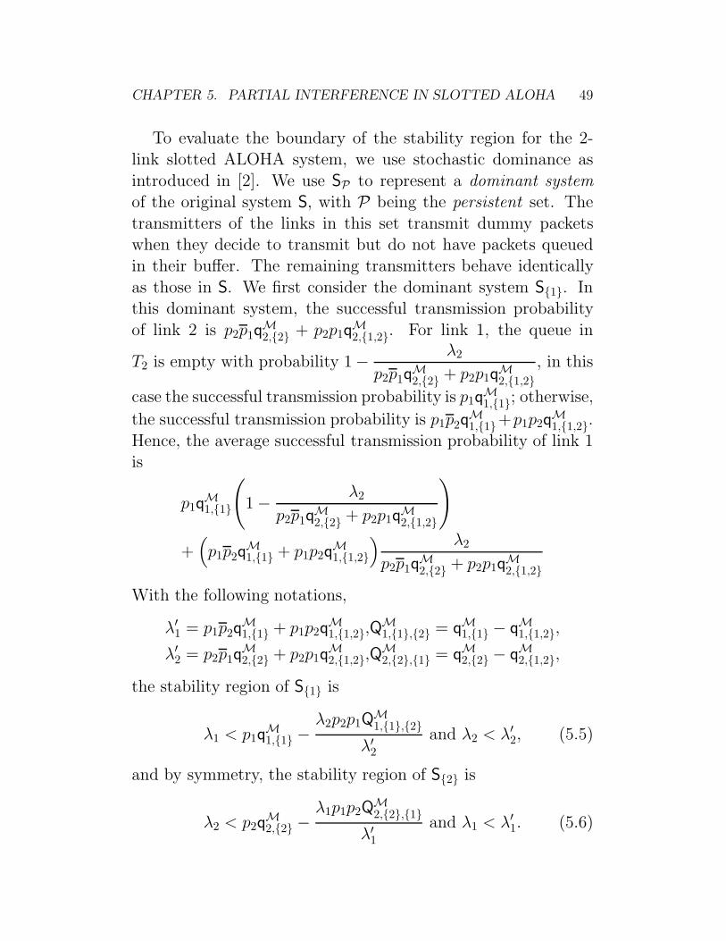
CHAPTER 5. PARTIAL INTERFERENCE IN SLOTTED ALOHA 49
To evaluate the boundary of the stability region for the 2-link slotted ALOHA system, we use stochastic dominance as
introduced in [2]. We use SP to represent a dominant systemof the original system S, with P being the persistent set. The
transmitters of the links in this set transmit dummy packetswhen they decide to transmit but do not have packets queuedin their buffer. The remaining transmitters behave identically
as those in S. We first consider the dominant system S1. Inthis dominant system, the successful transmission probability
of link 2 is p2p1qM2,2 + p2p1q
M2,1,2. For link 1, the queue in
T2 is empty with probability 1− λ2
p2p1qM2,2 + p2p1q
M2,1,2
, in this
case the successful transmission probability is p1qM1,1; otherwise,
the successful transmission probability is p1p2qM1,1+p1p2q
M1,1,2.
Hence, the average successful transmission probability of link 1is
p1qM1,1
(
1− λ2
p2p1qM2,2 + p2p1q
M2,1,2
)
+(
p1p2qM1,1 + p1p2q
M1,1,2
) λ2
p2p1qM2,2 + p2p1q
M2,1,2
With the following notations,
λ′1 = p1p2qM1,1 + p1p2q
M1,1,2,Q
M1,1,2 = qM1,1 − qM1,1,2,
λ′2 = p2p1qM2,2 + p2p1q
M2,1,2,Q
M2,2,1 = qM2,2 − qM2,1,2,
the stability region of S1 is
λ1 < p1qM1,1 −
λ2p2p1QM1,1,2
λ′2and λ2 < λ′2, (5.5)
and by symmetry, the stability region of S2 is
λ2 < p2qM2,2 −
λ1p1p2QM2,2,1
λ′1and λ1 < λ′1. (5.6)

CHAPTER 5. PARTIAL INTERFERENCE IN SLOTTED ALOHA 50
Table 5.1: Parameters used for the analytical results of slotted ALOHA.
P1, P2 24.5 dBm N1, N2 -88 dBm
GT , GR 1 hT , hR 1.5 m
ε 0.001 dT1,R1, dT2,R2
450 m
The union of these two regions constitutes the inner bound on
the stability region of the original system S.The reason for the union of these two regions to be the outer
bound on the stability region follows from the indistinguishabil-ity argument [2, 10]. Consider the dominant system S1. With
a particular initial condition on the length of the queues, if thequeue in T1 is unstable, it is equivalent to the case that thequeue in T1 never empties with nonzero probability. Then S1and S will be indistinguishable, in the sense that the packetstransmitted from T1 in S1 are always real packets, and S is
also unstable. Therefore, the union of the regions defined by(5.5) and (5.6) is the exact stability region for M = 2.
5.4 Some Illustrations
In this Section, we depict the stability region derived in previousSection by considering the parallel-link topology in Fig. 5.1. We
use the two-ray ground reflection model
pl(d) =GTGRh
2Th
2R
d4
to represent the path loss as in Chapter 3. The values of variousparameters are shown in Table 5.1.
We first assume L = 8192 bits, p1 = p2 = 0.8 and varythe link separation, i.e., the perpendicular distance betweenthe links, to obtain the results under binary interference in Fig.
5.2(a). The stability region has only two possible shapes. Forthe separations of 600, 800 and 1000 meters, the SNR attained

CHAPTER 5. PARTIAL INTERFERENCE IN SLOTTED ALOHA 51
T1
R1
T2
R2
Figure 5.1: A sample topology.
at either receiver when both transmitters are active is smallerthan the threshold. Therefore the underlying channel follows
the collision channel model and the stability region is noncon-vex. When the separation is 1200 meters, the links are separated
far enough so that transmissions on both links are independent.The channel can be regarded as the orthogonal channel and thestability region is convex. Therefore, the threshold in binary in-
terference determines when to switch between the collision chan-nel and the orthogonal channel.
Fig. 5.2(b) shows the corresponding results under partialinterference. When the link separation is small, the amount
of interference is so large that partial interference degeneratesto the collision channel. As the link separation increases, the
stability region expands gradually and changes from nonconvexto convex. At another extreme, when the links are sufficiently farapart, partial interference is identical to the orthogonal channel.
Therefore, partial interference can be viewed as a generalizationof binary interference that it interpolates the transition from
the collision channel to the orthogonal channel. Notice thatthe results here are similar to the case considered in Chapter
4, therefore our results should be applicable to networks withpractical random access protocols like 802.11.
Next, we assume the links are separated by 800 meters. We
let both links transmit with probability p, and illustrate the ef-fect of p on the convexity of the stability region under binary
interference in Fig. 5.3(a). When p is small, i.e., 0.2 and 0.4,the links are too conservative in attempting transmissions. It

CHAPTER 5. PARTIAL INTERFERENCE IN SLOTTED ALOHA 52
0 0.2 0.4 0.6 0.8 10
0.2
0.4
0.6
0.8
1
Loading on Link 1
Load
ing
on L
ink
2
Stability Region of Slotted Aloha under Binary Interference
dist=600mdist=800mdist=1000mdist=1200m
(a) binary interference.
0 0.2 0.4 0.6 0.8 10
0.2
0.4
0.6
0.8
1
Loading on Link 1
Load
ing
on L
ink
2
Stability Region of Slotted Aloha under Partial Interference
dist=600mdist=800mdist=1000mdist=1200m
(b) partial interference.
Figure 5.2: Stability region for M = 2 with transmission probabilities 0.8under binary and partial interference.
0 0.2 0.4 0.6 0.8 10
0.2
0.4
0.6
0.8
1
Loading on Link 1
Load
ing
on L
ink
2
Stability Region of Slotted Aloha under Binary Interference
p=0.20p=0.40p=0.60p=0.80
(a) binary interference.
0 0.2 0.4 0.6 0.8 10
0.2
0.4
0.6
0.8
1
Loading on Link 1
Load
ing
on L
ink
2
Stability Region of Slotted Aloha under Partial Interference
p=0.20p=0.40p=0.60p=0.80
(b) partial interference.
Figure 5.3: Stability region for M = 2 with link separation 800 meters underbinary and partial interference.
leads to better channel utilization by adding one more link tothe system, and the stability region is convex. On the otherhand, when p is large, i.e., 0.6 and 0.8, the links are too aggres-
sive. When one more link is added to the system, it increasescontention and hence reduces the loading supported by each link
drastically. As a result, the stability region is nonconvex. Theconvexity of the stability region can therefore be regarded as a
measure of the contention level in a network.Fig. 5.3(b) illustrates the stability region when partial inter-
ference is considered instead, under the same settings. Althoughthe SNR attained at a receiver when both transmitters are activeis smaller than the threshold, the SNR is large enough to sup-
port a sustainable throughput probabilistically. Therefore, it is

CHAPTER 5. PARTIAL INTERFERENCE IN SLOTTED ALOHA 53
0 0.2 0.4 0.6 0.8 10
0.2
0.4
0.6
0.8
1
Loading on Link 1
Load
ing
on L
ink
2
Stability Region of Slotted Aloha
partial interferencebinary interference
(a) p1 = p2 = 0.2.
0 0.2 0.4 0.6 0.8 10
0.2
0.4
0.6
0.8
1
Loading on Link 1
Load
ing
on L
ink
2
Stability Region of Slotted Aloha
partial interferencebinary interference
(b) p1 = p2 = 0.4.
0 0.2 0.4 0.6 0.8 10
0.2
0.4
0.6
0.8
1
Loading on Link 1
Load
ing
on L
ink
2
Stability Region of Slotted Aloha
partial interferencebinary interference
(c) p1 = p2 = 0.6.
0 0.2 0.4 0.6 0.8 10
0.2
0.4
0.6
0.8
1
Loading on Link 1
Load
ing
on L
ink
2
Stability Region of Slotted Aloha
partial interferencebinary interference
(d) p1 = p2 = 0.8.
Figure 5.4: Stability region for M = 2 under binary interference and partialinterference with various transmission probabilities.
possible to receive more packets opportunistically by exploitingpartial interference, thereby increasing the loading supported byeach link and allowing the stability region to be convex. If we
compare the stability region under binary and partial interfer-ence in identical settings, as shown in Figs. 5.4(a)-5.4(d), the
stability region under partial interference is always larger thanthat under binary interference. This implies that by consider-
ing partial interference, more combinations of flows on the linkscan be admitted, and the capacity of a wireless network can bepotentially increased.
5.5 Generalization to the M-Link Case
In this Section, we give in closed form a partial characteriza-
tion on the boundary of the stability region of M -link slotted

CHAPTER 5. PARTIAL INTERFERENCE IN SLOTTED ALOHA 54
ALOHA under partial interference. First, for n ∈ A ⊆ M,
γMn,A =PnCd
−αTn,Rn
∑
n′∈A\nPn′Cd−α
Tn′,Rn+Nn
. Therefore, under binary inter-
ference,
qMn,A =
1, γMn,A ≥ γ0
0, γMn,A < γ0
, (5.7)
while under partial interference,
qMn,A =[
1− e(
γMn,A
)]L
. (5.8)
For each M′ ⊆ M, let pM(M′) =(
pMn (M′))
n∈M be a M -dimensional 0-1 vector such that
pMn (M′) =
1, n ∈M′
0, n /∈M′ ,
where M′ is a set of persistent links and all other links are
empty. Define ΠpM(M′) =(
ΠpM(M′)n
)
n∈M, where
ΠpM(M′)n =
∑
A : n∈A⊆M′
∏
n′∈Apn′
∏
n′′∈M′\Apn′′qMn,A, (5.9)
to be a corner point corresponding to the case that M′ is theset of persistent links. Notice RHS of (5.9) is zero when n /∈M′.Then we obtain the following Theorem.
Theorem 5.1. All corner points lie on the boundary of the sta-bility region.
Proof. When M′ = ∅, (5.9) becomes ΠpM(M′) = 0, which is ob-
viously on the boundary. IfM′ 6= ∅, each link n ∈M′ operatesas M/M/1. If at a certain instant, only the links in A ⊆ M′
are active, which occurs with probability∏
n′∈Apn′
∏
n′′∈M′\Apn′′, the

CHAPTER 5. PARTIAL INTERFERENCE IN SLOTTED ALOHA 55
probability of successful transmission of link n is qMn,A. There-
fore, by unconditioning on A while noticing qMn,A = 0 if n /∈ A,the successful transmission probability of link n is
∑
A : n∈A⊆M′
∏
n′∈Apn′
∏
n′′∈M′\Apn′′qMn,A.
Therefore ΠpM(M′) lies on the boundary.
By using stochastic dominance and the indistinguishability
argument, we obtain the following Theorem.
Theorem 5.2. Let ΠpM(P),ΠpM(P∪D) be two corner points such
that D = n ⊆ M \ P. Then the line segment joining thesetwo points lies on the boundary of the stability region. This line
segment represents the case that P is the set of persistent linkswhile n is the only non-empty non-persistent link in the system.
Proof. When |P| = 0, it is trivial that the line segment between
ΠpM(P) and ΠpM(P∪D) lies on the boundary because it is part ofthe positive λn-axis. Assume |P| > 0. We prove
λn < λ′n, n ∈ D,λn <
∑
A : n∈A⊆P
∏
n′∈Apn′
∏
n′′∈P\Apn′′qMn,A
−λn
λ′npn
∑
A : n∈A⊆P
∏
n′∈Apn′
∏
n′′∈P\Apn′′QMn,A,D, n ∈ P,
λn = 0, n ∈M \ (P ∪ D) (5.10)
with
λ′n =∑
A : n∈A⊆(P∪D)
∏
n′∈Apn′
∏
n′′∈(P∪D)\Apn′′qMn,A,
QMn,A,D = qMn,A − qMn,A∪D,A : n ∈ A ⊆ P .
lies on the boundary of the stability region. For any n /∈ P ∪D,
Tn has no packet, hence λn = 0. Therefore we consider the

CHAPTER 5. PARTIAL INTERFERENCE IN SLOTTED ALOHA 56
dominant system SP , assuming the system contains only thelinks in P ∪ D. For the sufficiency part, the queue in Tn in SPis stable if
λn < pn
∑
A⊆P
∏
n′∈Apn′
∏
n′′∈P\Apn′′qMn,A∪D
=∑
A : n∈A⊆(P∪D)
∏
n′∈Apn′
∏
n′′∈(P∪D)\Apn′′qMn,A = λ′n
For any n ∈ P, the queue in Tn in SP is stable if
λn <
(
1− λn
λ′n
)
∑
A : n∈A⊆P
∏
n′∈Apn′
∏
n′′∈P\Apn′′qMn,A
+λn
λ′n
∑
A : n∈A⊆(P∪D)
∏
n′∈Apn′
∏
n′′∈(P∪D)\Apn′′qMn,A
=
(
1− λn
λ′n
)
∑
A : n∈A⊆P
∏
n′∈Apn′
∏
n′′∈P\Apn′′qMn,A
+λn
λ′n
(
pn
∑
A : n∈A⊆P
∏
n′∈Apn′
∏
n′′∈P\Apn′′qMn,A
+pn
∑
A : n∈A⊆P
∏
n′∈Apn′
∏
n′′∈P\Apn′′qMn,A∪D
)
=∑
A : n∈A⊆P
∏
n′∈Apn′
∏
n′′∈P\Apn′′qMn,A
−λn
λ′npn
∑
A : n∈A⊆P
∏
n′∈Apn′
∏
n′′∈P\Apn′′QMn,A,D
The necessity follows directly from the indistinguishability argu-
ment. We observe that λn varies linearly with λn on the bound-ary, ∀n /∈ D. It is trivial that λn = 0 and λn = λ′n correspondto ΠpM(P) and ΠpM(P∪D) respectively.
We illustrate the results of these Theorems by considering

CHAPTER 5. PARTIAL INTERFERENCE IN SLOTTED ALOHA 57
−200 0 200 400 600 800 1000 1200 1400−800
−600
−400
−200
0
200
400
600
800
1000
1200
T1
R1
T2R2
T3
R3
(a) A sample topology.
0
0.5
1
00.5
1
0
0.2
0.4
0.6
0.8
1
Loading on Link 1
Stability Region of Slotted Aloha
Loading on Link 2
Load
ing
on L
ink
3
Π(0,0,0)
Π(1,0,0)
Π(0,1,0)
Π(1,1,0)
Π(0,0,1)
Π(1,0,1)
Π(0,1,1)
Π(1,1,1)
(b) Part of the exact boundary.
Figure 5.5: Stability region with M = 3.
M = 3 with the ring topology in Fig. 5.5(a). The distance be-tween a receiver and the nearest interfering transmitter is 900
meters. Each link transmits with probability 0.6. Other param-eters are the same as in Table 5.1. From Theorem 5.1, each of
the eight 3-dimensional 0-1 vector corresponds to a corner pointshown in Fig. 5.5(b), and their coordinates can be obtainedfrom (5.9). By Theorem 5.2, the solid lines in Fig. 5.5(b) are
part of the boundary of the stability region. As another exam-ple, for M = 2, notice that (5.5) and (5.6) are special cases of
(5.10). As a direct consequence of our Theorems 5.1 and 5.2, thestability region of slotted ALOHA with two links under partial
interference is piecewise linear.Theorems 5.1 and 5.2 cover all cases with zero or one non-
empty non-persistent link in the system respectively. However,
if there are at least two non-empty non-persistent links, the sta-tionary joint queue statistics must be involved in calculating the
boundary. Hence, the results here are the best we can obtainwithout the stationary joint queue statistics. Unless we are able
to compute the stationary joint queue statistics in closed-form,we are unable to solve the capacity-finding problem, even assum-
ing the simplest random access protocol, i.e., slotted ALOHA.

CHAPTER 5. PARTIAL INTERFERENCE IN SLOTTED ALOHA 58
5.6 Chapter Summary
We have studied the stability problem of finite-link infinite-buffer slotted ALOHA and derived the exact stability region
when there are two links in the network under partial interfer-ence. We illustrated that under partial interference, there is onecommon property for the stability regions of 802.11 and slotted
ALOHA: the stability region expands gradually as the separa-tion between the links increases. When there are more than two
links in the network, we only obtained part of the boundary ofthe stability region. Even for the case of collision channel, we
still cannot obtain the exact stability region, because it involvesthe stationary joint queue statistics which do not have closedform to date. Therefore, for both 802.11 and slotted ALOHA,
we cannot analytically establish the boundary of the stabilityregion.
2 End of chapter.

Chapter 6
FRASA
6.1 Introduction
In previous two Chapters, we attempted to find the boundaryof the stability regions of 802.11 and slotted ALOHA networks
respectively. However, there is only limited success for bothtasks. For 802.11, the boundary of the stability region is com-puted numerically; while for slotted ALOHA, only part of the
boundary can be obtained analytically. Therefore, instead offinding an analytically tractable boundary of the stability re-
gion of wireless random access networks, we have to resort toapproximation.
In this Chapter, we propose FRASA, Feedback Retransmis-sion Approximation for Slotted ALOHA, to study the stabil-ity region of finite-link slotted ALOHA under collision channel.
With FRASA, we derive in closed form the boundary of thestability region for any number of links in the system. The re-
sult derived from FRASA is identical to the analytical result offinite-link slotted ALOHA when there are two links in the sys-
tem. Simulation shows that the stability region obtained fromFRASA is a good approximation to the stability region of finite-
link slotted ALOHA. FRASA also has a wider range of applica-bility than the bounds derived in previous researches. We pro-vide a convex hull bound, which is convex, piecewise linear and
59
CHAPTER 6. FRASA 60
outer-bounds the stability region of FRASA. This bound canbe computed by using the transmission probability vector only.
We also characterize p-convexity, an essential property that thestability region of FRASA should have to ensure the convex hull
bound to be close to the boundary. From this, we derive thatthe stability region of FRASA can never be convex when thereare more than two links in the system. A convex and piecewise
linear inner bound on the stability region of FRASA, called thesupporting hyperplane bound, is also given. Furthermore, we ex-
tend the results of FRASA to include other interference modelslike binary and partial interference. The analytical findings with
FRASA can also provide more insights on the characterizationof the capacity region of other types of wireless random access
networks.
6.2 The FRASA Model
In slotted ALOHA, there is a queue of infinite buffer at each
transmitter. Packet arrivals are assumed to be Bernoulli. Whena packet arrives, it joins the end of the queue. The head-of-linepacket is transmitted when the transmitter decides to transmit,
and it remains at head-of-line until it is successfully transmitted.This is depicted in the upper part of Fig. 6.1.
Due to the complexity introduced by the queues, we pro-pose FRASA, Feedback Retransmission Approximation for Slot-
ted ALOHA, as a surrogate to approximate finite-link slottedALOHA. In FRASA, the buffer in each transmitter can hold
one packet only. Whenever there is a packet in the buffer, if thetransmitter decides not to transmit the packet, or the transmit-ter cannot successfully transmit the packet due to collision, the
packet will be removed from the buffer and put back in the bufferagain after a random delay which is geometrically distributed.
Therefore, the aggregate arrival of packets to the buffer, which

CHAPTER 6. FRASA 61
Random Delay
Figure 6.1: Slotted ALOHA model: (Upper) Original; (Lower) FRASA.
is defined as the sum of the new arrivals and the retransmissions,
is assumed to be Bernoulli or memoryless. Similar approxima-tion was introduced by [25]. FRASA is shown in the lower partof Fig. 6.1.
Assume there are M links in the network, and the set oflinks is denoted by M = nMn=1. Denote this FRASA system
by S. Let p = (pn)n∈M be the transmission probability vector.Define pn = 1 − pn for all n ∈ M. We first consider a reduced
FRASA system, in which we let M − 1 of the links have fixedaggregate arrival rates and the remaining link is assumed with
infinite backlog. Take n ∈M to be the link with infinite backlogand denote this reduced FRASA system by Sn. Let χn be theaggregate arrival rate of link n ∈M \ n where χn is between
zero and one. Hence, link n is active with probability pn, whilefor n 6= n, link n is active with probability χnpn. Therefore,
λ =(
λn
)
n∈M is the successful transmission probability vectorand
λn =
χnpn(1− pn)∏
n′∈M\n,n(1− χn′pn′), n 6= n
pn
∏
n′∈M\n(1− χn′pn′), n = n
, (6.1)
with λn > 0. We use the results from [24] to determine when
Sn is stable as in Chapter 5: on the assumption that the arrival

CHAPTER 6. FRASA 62
and the service processes of a queue are stationary, the queue isstable if the average arrival rate is less than the average service
rate, and the queue is unstable if the average arrival rate islarger than the average service rate. Then, λn = λn, ∀n ∈ M is
the parametric form of the boundary of the stability region ofSn. We can obtain a non-parametric version by using (6.1) asfollows.
Lemma 6.1. Consider Sn. When
λn(1− pn)
pn
≥ λn(1− pn)
pn
≥ 0 (6.2)
is satisfied for all n ∈M \ n, the hypersurface Fn, i.e.,
∏
n′∈M[λn(1− pn) + λn′pn] = pn[λn(1− pn)]
M−1 (6.3)
is the non-parametric form of the boundary of the stability region
of Sn.
Proof. Starting from the parametric form (6.1), for n ∈M\n,
λn
λn
=
χnpn(1− pn)∏
n′∈M\n,n(1− χn′pn′)
pn
∏
n′∈M\n(1− χn′pn′)
=χnpn(1− pn)
pn(1− χnpn)
Therefore,
χn =λnpn
λn(1− pn)pn + λnpnpn
and the condition 0 ≤ χn ≤ 1 is translated into
λn(1− pn)
pn
≥ λn(1− pn)
pn
≥ 0.

CHAPTER 6. FRASA 63
Combining these results,
λn = pn
∏
n′∈M\n(1− χn′pn′)
= pn
∏
n′∈M\n
[
1− λn′pnpn′
λn(1− pn)pn′ + λn′pnpn′
]
= pn
∏
n′∈M\n
λn(1− pn)
λn(1− pn) + λn′pn
,
we obtain∏
n′∈M[λn(1− pn) + λn′pn] = pn[λn(1− pn)]
M−1
as the boundary of the stability region of Sn.
Recall the system is stable if all queues in the system are
stable [3, 10, 14], and notice the expressionλn(1− pn)
pn
in (6.2)
is identical to the instability rank introduced in [3]. When
maxn∈M
λn(1− pn)
pn
=λn(1− pn)
pn
holds as in (6.2), link n is the
most probable one to be the first unstable link. Hence, we letlink n to be infinitely backlogged and use Lemma 6.1 to obtain
the stability region of FRASA as in the following Theorem.
Theorem 6.1. R =⋃
n∈MRn is the stability region of FRASA,
where Rn is represented by:
λn(1− pn)
pn
≥ λn(1− pn)
pn
≥ 0, ∀n ∈M \ n, (6.4)∏
n′∈M[λn(1− pn) + λn′pn] < pn[λn(1− pn)]
M−1. (6.5)
The union here is actually a disjoint union.

CHAPTER 6. FRASA 64
Proof. By (6.4), the positive orthant is partitioned into M re-
gions. In the region that maxn∈M
λn(1− pn)
pn
=λn(1− pn)
pn
, link n
is the most probable one to be the first link to become unsta-
ble, therefore we let link n be the only link with infinite backlog(in case there are more than one n that maximize the instabil-ity rank, choose one of them to be n arbitrarily). Then from
Lemma 6.1,∏
n′∈M[λn(1− pn) + λn′pn] = pn[λn(1− pn)]
M−1
is the boundary of the stability region of FRASA. Consider apoint λ = (λn)n∈M in M -dimensional space where λn < pn
and λn = 0, ∀n ∈ M \ n. This point lies inside the stabil-
ity region of FRASA. Substituting into the above equation, weget λn[λn(1 − pn)]
M−1 on LHS and pn[λn(1 − pn)]M−1 on RHS.
Therefore, when (6.4) holds,∏
n′∈M[λn(1− pn) + λn′pn] < pn[λn(1− pn)]
M−1
is the condition for the reduced FRASA system Sn to be stable.Thus, the region formed by (6.4) and (6.5) is part of the stability
region of S. By taking the union over all possible values of n,we obtain the stability region of FRASA.
We first illustrate our results for M = 2. When
λ1(1− p1)
p1≥ λ2(1− p2)
p2≥ 0
holds, the boundary of the stability region of FRASA is
λ1[λ1(1− p1) + λ2p1] = p1λ1(1− p1),
which is reduced to
λ1 = p1
(
1− λ2
1− p1
)

CHAPTER 6. FRASA 65
Figure 6.2: Stability region with M = 2: (Upper) From [2]; (Lower) FromFRASA.
after simplification. Geometrically, it is a straight line joiningthe points (p1, 0) and (p1p2, p2p1). This is depicted in the bottom
left of Fig. 6.2. By symmetry, we also get
λ2 = p2
(
1− λ1
1− p2
)
as the boundary of the stability region of FRASA when
λ2(1− p2)
p2≥ λ1(1− p1)
p1≥ 0
holds. This is a straight line joining the points (0, p2) and
(p1p2, p2p1). This is shown in the bottom center of Fig. 6.2.The bottom right of Fig. 6.2 contains the final result of the sta-
bility region obtained from FRASA. The stability region derivedin [2] is illustrated in the top row of Fig. 6.2 for comparison.We see that the final results are identical to each other.
Next we consider the case of M = 3 and each link has atransmission probability of 0.3. Figs. 6.3(a), 6.3(b) and 6.3(c)
illustrate the results of Lemma 6.1 for S1, S2 and S3 respec-tively. The single-colored hyperplanes in Figs. 6.3(a), 6.3(b)

CHAPTER 6. FRASA 66
00.1
0.20.3
0
0.1
0.2
0.3
0
0.1
0.2
0.3
Loading on Link 1Loading on Link 2
Load
ing
on L
ink
3
(a) R1, stability region with link 1having maximum instability rank.
0
0.1
0.2
0.3
00.1
0.20.3
0
0.1
0.2
0.3
Loading on Link 1Loading on Link 2
Load
ing
on L
ink
3
(b) R2, stability region with link 2having maximum instability rank.
00.1
0.20.3
00.1
0.20.3
0
0.1
0.2
0.3
Loading on Link 1Loading on Link 2
Load
ing
on L
ink
3
(c) R3, stability region with link 3having maximum instability rank.
0
0.1
0.2
0.3
0
0.1
0.2
0.3
0
0.1
0.2
0.3
Loading on Link 1Loading on Link 2
Load
ing
on L
ink
3
(d) R, the whole stability region.
Figure 6.3: Stability region of FRASA with M = 3 and transmission proba-bilities 0.3 by Lemma 6.1 and Theorem 6.1.
and 6.3(c) form the partition of the positive orthant generated
by (6.2), while the multi-colored hypersurfaces come from (6.3).The union of these regions constitutes the stability region in Fig.6.3(d) as stated in Theorem 6.1. Another example is shown in
Figs. 6.4(a)-6.4(d), in which each link transmits with probabil-ity 0.6.
6.3 Validation of the FRASA Model
6.3.1 Simulation Results
In this Section, we first use simulation to verify if FRASA is agood approximation to finite-link slotted ALOHA. Since whenM = 2, we obtain identical results for both FRASA and finite-

CHAPTER 6. FRASA 67
00.2
0.40.6
0
0.2
0.4
0.6
0
0.2
0.4
0.6
Loading on Link 1Loading on Link 2
Load
ing
on L
ink
3
(a) R1, stability region with link 1having maximum instability rank.
0
0.2
0.4
0.6
00.2
0.40.6
0
0.2
0.4
0.6
Loading on Link 1Loading on Link 2
Load
ing
on L
ink
3
(b) R2, stability region with link 2having maximum instability rank.
00.2
0.40.6
00.2
0.40.6
0
0.2
0.4
0.6
Loading on Link 1Loading on Link 2
Load
ing
on L
ink
3
(c) R3, stability region with link 3having maximum instability rank.
0
0.2
0.4
0.6
0
0.2
0.4
0.6
0
0.2
0.4
0.6
Loading on Link 1Loading on Link 2
Load
ing
on L
ink
3
(d) R, the whole stability region.
Figure 6.4: Stability region of FRASA with M = 3 and transmission proba-bilities 0.6 by Lemma 6.1 and Theorem 6.1.
link slotted ALOHA, we consider M = 3 here.
First, to check whether the slotted ALOHA system is stableor not by simulation, we extend the algorithm proposed in [26].This is stated as Algorithm 1.
In this algorithm, for each simulation run, we partition thesimulation time into N batches, where N ≥ 2. We calculate
the average queue lengths for each batch, Qn,w(b), starting fromthe second batch (Line 2). We discard the first batch to remove
any transient behavior in the system. Then we compute thesample mean and sample variance of the average queue length,i.e., E
[
Qn,w
]
and V ar(
Qn,w
)
, respectively (Lines 3-4). We use
the difference between the last and the second observation, i.e.,

CHAPTER 6. FRASA 68
Algorithm 1 Stability Checking
Require: number of batches: N ≥ 2Require: probability of type I error: a
Require: number of slots: TRequire: simulation runs: W oddRequire: queue lengths: Qn,w(t), t ≤ T , n ∈M, 1 ≤ w ≤ W1: B ← TN2: Qn,w(b)← 1
BbB∑
t=(b−1)B+1
Qn,w(t), 2 ≤ b ≤ N , n ∈M, 1 ≤ w ≤ W
3: E[
Qn,w
]
← 1
N − 1
N∑
b=2
Qn,w(b), n ∈M, 1 ≤ w ≤ W
4: V ar(
Qn,w
)
← 1
N − 2
N∑
b=2
Qn,w(b)− E[
Qn,w
]
2
, n ∈M, 1 ≤ w ≤ W
5: Qn,w ← Qn,w(N )−Qn,w(2), n ∈M, 1 ≤ w ≤ W6: for w = 1 to W do
7: ifQn,w
√
2V ar(
Qn,w
)
> t1−a,N−2, ∃n ∈M then
8: Xw = 09: else
10: Xw = 111: end if12: end for
13: ifW∑
w=1
Xw >W2
then
14: output STABLE15: else16: output UNSTABLE17: end if

CHAPTER 6. FRASA 69
Qn,w, in the hypothesis testing (Line 5). If,
Qn,w√
2V ar(
Qn,w
)
> t1−a,N−2, ∃n ∈M, (6.6)
where t1−a,N−2 is the (1-a)-percentile of t-distribution withN−2degrees of freedom, is satisfied, we assume the system is unsta-ble; otherwise all queues in the slotted ALOHA system is stable
and so does the system (Lines 7-11). If the system is unsta-ble, there must exist n ∈M such that the length of queue n has
positive linear growth rate, making the hypothesis (6.6) satisfiedwith high probability. Otherwise, the expectation of Qn,w would
be zero for all n ∈ M, and with high probability (6.6) wouldbe false. We perform W simulation runs and then use major-ity vote to determine whether the system is stable (Line 13-17),
therefore we require W to be odd. More than one simulationruns are performed in order to reduce the error in simulations.
Using Algorithm 1 as a subroutine, we use the following ap-proach to find the boundary of the stability region, which is
stated as Algorithm 2.This algorithm is based on bisection method [22]. We let
λ1 and λ2 increase from zero to one (Line 1-2). Given anyp = (p1, p2, p3), for any λ1 and λ2 between zero and one, let theinitial search range of λ3 be [0, 1] and set λ3 to be the midpoint
of the search range. Then we let λ = (λ1, λ2, λ3) be the arrivalprobabilities of the links and simulate the slotted ALOHA sys-
tem (Line 6). We use Algorithm 1 to check the stability of thequeues in the system and conclude the stability of the system. If
Algorithm 1 indicates that the system is stable, we set the nextsearch range of λ3 to be the upper half of the original one (Line8); otherwise, we use the lower half as the next search range
(Line 10). We iterate until the search range is sufficiently small(Line 5). Then we take the midpoint of the final search range
to be the boundary value of λ3 for the given values of λ1 and

CHAPTER 6. FRASA 70
Algorithm 2 Stability Region Boundary Generation
Require: 0 ≤ p1, p2, p3 ≤ 1Require: δ > 01: for λ1 = 0 to 1 in step 0.01 do2: for λ2 = 0 to 1 in step 0.01 do3: λ3 ← 0.54: δ ← 0.255: while δ ≥ δ do6: perform W simulation runs7: if Algorithm 1 returns STABLE then8: λ3 ← λ3 + δ9: else
10: λ3 ← λ3 − δ11: end if
12: δ ← δ
213: end while14: end for15: end for
Table 6.1: Parameters used for the simulations.N 2 a 0.05
T 4000 W 3
t1−a,N−2 1.8595 δ 0.001
λ2. We repeat this procedure for any combination of λ1 and λ2
to get the boundary of the stability region. The values of the
parameters used in these algorithms are shown in Table 6.1.For illustrative purposes, we only show the cross-sections of
the stability regions. We first let all links transmit with probabil-
ity 0.3. In Fig. 6.5(a) we depict the cross-sections of the stabilityregion by fixing λ2, while in Fig. 6.5(b) the cross-sections of the
stability region are obtained by fixing λ1. The solid lines repre-sent the simulation results while the dash-dot lines are obtained
from FRASA. In Figs. 6.6(a) and 6.6(b) we show the corre-sponding results by changing the transmission probabilities ofall links to 0.6. We observe that there is a close match between

CHAPTER 6. FRASA 71
0 0.1 0.2 0.3 0.40
0.05
0.1
0.15
0.2
0.25
0.3
0.35
0.4
Loading on Link 1
Load
ing
on L
ink
3
Slices of Stability Region of Slotted Aloha
Load 2 = 0.00 SLoad 2 = 0.00 ALoad 2 = 0.10 SLoad 2 = 0.10 ALoad 2 = 0.20 SLoad 2 = 0.20 A
(a) λ2 fixed.
0 0.1 0.2 0.3 0.40
0.05
0.1
0.15
0.2
0.25
0.3
0.35
0.4
Loading on Link 2
Load
ing
on L
ink
3
Slices of Stability Region of Slotted Aloha
Load 1 = 0.00 SLoad 1 = 0.00 ALoad 1 = 0.10 SLoad 1 = 0.10 ALoad 1 = 0.20 SLoad 1 = 0.20 A
(b) λ1 fixed.
Figure 6.5: Cross-section of stability region with M = 3 and transmissionprobabilities 0.3.
0 0.1 0.2 0.3 0.4 0.5 0.60
0.1
0.2
0.3
0.4
0.5
0.6
Loading on Link 1
Load
ing
on L
ink
3
Slices of Stability Region of Slotted Aloha
Load 2 = 0.00 SLoad 2 = 0.00 ALoad 2 = 0.20 SLoad 2 = 0.20 ALoad 2 = 0.40 SLoad 2 = 0.40 A
(a) λ2 fixed.
0 0.1 0.2 0.3 0.4 0.5 0.60
0.1
0.2
0.3
0.4
0.5
0.6
Loading on Link 2
Load
ing
on L
ink
3
Slices of Stability Region of Slotted Aloha
Load 1 = 0.00 SLoad 1 = 0.00 ALoad 1 = 0.20 SLoad 1 = 0.20 ALoad 1 = 0.40 SLoad 1 = 0.40 A
(b) λ1 fixed.
Figure 6.6: Cross-section of stability region with M = 3 and transmissionprobabilities 0.6.
the stability region of FRASA and the stability region of slotted
ALOHA. In FRASA, we introduce the parameter χnn∈M\nto compute the boundary of the stability region. χnn∈M\n inFRASA can be regarded as the stationary joint queue statistics,
which are essential for computing the boundary of the stabilityregion of slotted ALOHA as stated in Chapter 5. Therefore, the
stability region of FRASA is a good approximation to the sta-bility region of slotted ALOHA, in the sense that we compute
the stability region of slotted ALOHA by assuming we know thestationary joint queue statistics.

CHAPTER 6. FRASA 72
6.3.2 Comparison to Previous Bounds
Here, we demonstrate that FRASA is a good approximation
to finite-link slotted ALOHA by showing the boundary valuesobtained from FRASA lie inside the upper and lower bounds
in [3]. We fix the loading of the first M − 1 links, evaluatethe “FRASA” value of λM , and evaluate the “Upper” bound
and “Lower” bound of λM by using Theorems 3 and 5 in [3]respectively. Before showing this, we point out that the bounds
in [3] are applicable only when the instability rank assumption,i.e., link M has the highest instability rank, holds. This isbest illustrated by the following examples. Consider a slotted
ALOHA system with two links. We let both links transmitwith probability 0.6. We keep increasing λ1 while assumingλ1(1− p1)
p1≤ λ2(1− p2)
p2, and evaluate the upper bound on λ2
by using Theorem 3 in [3]. When λ1 > p1p2, the upper bound,
i.e., λ2,max, satisfiesλ2(1− p2)
p2≤ λ2,max(1− p2)
p2<λ1(1− p1)
p1,
showing that the instability rank assumption does not hold. Wechange the transmission probabilities of both links to 0.3 and
repeat the whole process, but evaluate the lower bound on λ2
by using Theorem 5 in [3]. It is found that when λ1 > p1p2, the
lower bound, i.e., λ2,min, satisfiesλ2,min(1− p2)
p2<
λ1(1− p1)
p1,
and we cannot conclude whether the instability rank assump-tion is valid or not. These results are depicted in Figs. 6.7(a)and 6.7(b) respectively. In the case of M = 2, we already have
the complete characterization on the boundary of the stabilityregion, therefore we can explicitly evaluate λ2 and show that
when λ1 > p1p2, the instability rank assumption does not hold,and the Theorems in [3] are not applicable. When M > 2, if
there are some λn satisfying λn > pn
∏
n′∈M\npn′, it is difficult

CHAPTER 6. FRASA 73
0 0.1 0.2 0.3 0.4 0.5 0.60
0.1
0.2
0.3
0.4
0.5
Loading on Link 1
Load
ing
on L
ink
2
Stability Region with p1=0.60, p2=0.60
ExactUpper Bound
(a)
0 0.05 0.1 0.15 0.2 0.25 0.30
0.05
0.1
0.15
0.2
0.25
Loading on Link 1
Load
ing
on L
ink
2
Stability Region with p1=0.30, p2=0.30
ExactLower Bound
(b)
Figure 6.7: Restricted application of the upper and lower bounds in [3].
to predict whether the instability rank assumption is valid or
not. When the instability rank assumption is not valid, onemay tempt to switch the order of the links to keep the validity
of the assumption. But in this case, we even cannot determinethe stability of the links with instability ranks higher than that
of link M , because the bounds on link n depend on the load-ings on the links having smaller instability ranks than link n [3].Therefore, when using the bounds in [3], we cannot set the load-
ings on the first M − 1 links too large in order to maintain theinstability rank assumption.
However, such restriction does not exist in computing the“FRASA” value of λM . We first let link M be the link with
the highest instability rank, i.e., n = M . Then we solve (6.3)for λM , which is an equation of degree M − 1, and get M − 1
values of λM . Exactly one of them is the desired value, whichmakes the instability rank of link M the highest. Otherwise, wefind the link with the highest instability rank among the first
M − 1 links. We let it equals n and solve (6.3) for λM , whichis an equation of degree one. In this case, we get a nonnegative
value which is the desired value of λM . Otherwise, we concludethat with the loadings on the first M − 1 links, it is impossible
to keep the system stable no matter how small λM is.To compare the numerical values computed from FRASA

CHAPTER 6. FRASA 74
against the bounds in [3], we consider the numerical examplesin [2] and [3]. The examples are reproduced in Tables 6.2-6.15.
The values of the loadings are classified into four groups in eachtable. In G1, one or more values of λn are zero. In G2, all λn are
approximately equal to1
2pn
∏
n′∈M\npn′. In G3, all λn are close to
pn
∏
n′∈M\npn′. In G4, one or more λn satisfy λn > pn
∏
n′∈M\npn′,
and these λn are marked with asterisks in the tables. In all cases,
the values predicted from FRASA lie inside the upper and lowerbounds in [3]. Simulations are also performed for all examplesin [2] and [3], and the results are shown in brackets in the ta-
bles. While the difference between the simulation result and thecorresponding “FRASA” value can be as large as 40% (the first
case of G4 in Table 6.3), for most cases, 82 (resp. 90) out of 96,the simulation results deviate from the corresponding “FRASA”
values by at most ±2% (resp. ±10%). The examples also showthat the bounds in [3] may not be always applicable, as in thecase of G4 in Table 6.5.
For the first case of G4 in Table 6.3, we plot the contourof the stability region of FRASA in Fig. 6.8 to investigate the
reason for such a large discrepancy between the stability regionof slotted ALOHA and FRASA. This contour plot shows that
when λ1 and λ2 are approximately equal to 0.035 and 0.0561respectively, the contour lines are very close together, meaning
that the boundary of the stability region at λ1 = 0.035 andλ2 = 0.0561 is almost parallel to the λ3-axis, i.e., the boundaryis very sensitive to small changes in λ1 and λ2. Therefore, in this
situation, it is difficult to obtain the boundary of the stabilityregion of slotted ALOHA by simulations.

CHAPTER 6. FRASA 75
0 0.1 0.2 0.3 0.4 0.5 0.60
0.1
0.2
0.3
0.4
0.5
0.6
Loading on Link 1Lo
adin
g on
Lin
k 2
Figure 6.8: Contour plot of the stability region of FRASA for the first caseof G4 in Table 6.3.
6.4 Convex Hull Bound
Although Theorem 6.1 gives us a closed-form expression for thestability region of FRASA, this stability region is not convex
when M > 2 (as shown in the next Section). Therefore weare motivated to derive outer and inner bounds on the stability
region of FRASA that are convex and piecewise linear, whichcan be used to find the upper and lower bounds on networkcapacity respectively. In this Section, we first develop an outer
bound on the stability region of FRASA that is guaranteed tobe convex and piecewise linear by using corner points of the
stability region of FRASA. For each M′ ⊆ M, we obtain a
corner point ΠpM(M′) =(
ΠpM(M′)n
)
n∈M, where
ΠpM(M′)n =
pn
∏
n′∈M′\npn′, n ∈M′
0, n ∈M \M′. (6.7)
These corner points, by construction, lie on the boundary ofthe stability region of FRASA because they satisfy the para-
metric form (6.1). We first obtain the following Lemma, statingthe relationship between the boundary of the stability region of
FRASA and the corner points.

CHAPTER 6. FRASA 76
Lemma 6.2. The boundary of the stability region of Sn, i.e., the
hypersurface Fn, is contained in the convex hull Hn generatedby the corner points ΠpM(M′∪n) for all M′ ⊆ M \ n, i.e.,every point satisfying (6.3) is a convex combination of the corner
points ΠpM(M′∪n) for all M′ ⊆M\ n.Proof. Let Π = (Πn)n∈M be a point satisfying (6.3). Then, from
the parametric form (6.1),
Πn =
χnpn(1− pn)∏
n′∈M\n,n(1− χn′pn′), n 6= n
pn
∏
n′∈M\n(1− χn′pn′), n = n
. (6.8)
If Π is a convex combination of ΠpM(M′∪n) for all M′ ⊆ M \n, then
Πn =
pnpn
∑
M′ : n∈M′⊆M\nφM′
∏
n′∈M′\npn′, n 6= n
pn
∑
M′⊆M\nφM′
∏
n′∈M′
pn′, n = n(6.9)
where∑
M′⊆M\nφM′ = 1 and φM′ ≥ 0, ∀M′ ⊆M \ n.
We will show that φM′M′⊆M\n always exists. When n = n,we get
∑
M′⊆M\nφM′
∏
n′∈M′
pn′ =∏
n′∈M\n(1− χn′pn′).
Consider this as a multinomial in pnn∈M\n. By equating the
coefficient of∏
n′∈M′′
pn′ for allM′′ ⊆M\ n, we get
∑
M′ :M′′⊆M′⊆M\nφM′ =
∏
n′∈M′′
χn′. (6.10)

CHAPTER 6. FRASA 77
Also by equating the coefficient of∏
n′∈M′′
pn′ for all M′′ ⊆ M \
n, n with n 6= n, we get∑
M′ : M′′∪n⊆M′⊆M\nφM′ = χn
∏
n′∈M′′
χn′.
Observe that this is only a special case of (6.10), it suffices to
consider (6.10) only. Notice that (6.10) is a system of linearequations. By Gaussian elimination, we see that for all M′′ ⊆M\ n,
φM′′ =∑
M′ : M′′⊆M′⊆M\n(−1)|M
′|−|M′′| ∏
n′∈M′′
χn′
=∏
n′∈M′′
χn′
∏
n′′∈M\(M′′∪n)(1− χn′′) ≥ 0.
Also, by consideringM′′ = ∅ in (6.10), we obtain∑
M′⊆M\nφM′ = 1.
Therefore, every point satisfying (6.3) is a convex combination
of ΠpM(M′∪n) for allM′ ⊆M\ n.By using Lemma 6.2 and Theorem 6.1, we obtain the follow-
ing Theorems about using convex hulls to bound the stabilityregion of FRASA. To obtain the bounds from these Theorems,
we only have to know the coordinates of all corner points, whichcan be computed from (6.7) based on the transmission proba-
bility vector only.
Theorem 6.2 (Bound of Convex-Hull Union). The convex hull
generated by ΠpM(M′∪n) for allM′ ⊆M\n together with 0,i.e., the origin, is a piecewise linear outer bound on Rn. Denote
this convex hull by Hn. Therefore, the union of these Hn for alln ∈ M, i.e., H =
⋃
n∈MHn, is a piecewise linear outer bound on
the stability region of FRASA. The union here is also disjoint.

CHAPTER 6. FRASA 78
Proof. Consider the reduced FRASA system Sn and let M′ ⊆M \ n. From (6.7), for every n ∈ M \ n, all corner points
ΠpM(M′∪n) with n ∈M′ and 0 lie on the boundaryλn(1− pn)
pn
=
λn(1− pn)
pn
, all corner points ΠpM(M′∪n) with n /∈M′∪n and
0 lie on the boundaryλn(1− pn)
pn
= 0. Also, for all n ∈M\n,the condition 0 ≤ χn ≤ 1 implies none of the corner points lie
outside the regionλn(1− pn)
pn
≥ λn(1− pn)
pn
≥ 0. Hence, for all
n ∈ M \ n, λn(1− pn)
pn
=λn(1− pn)
pn
andλn(1− pn)
pn
= 0 are
the boundaries of both Rn and Hn. Therefore, from Lemma 6.2,
Rn ⊆ Hn, and R =⋃
n∈MRn ⊆
⋃
n∈MHn = H. Since the bound-
ariesλn(1− pn)
pn
=λn(1− pn)
pn
andλn(1− pn)
pn
= 0 are linear
and the convex hull generated by a set of points is piecewiselinear, H is piecewise linear.
Theorem 6.3 (Convex Hull Bound). H, the convex hull gen-erated by ΠpM(M′) for all M′ ⊆ M, is a convex and piecewise
linear outer bound on the stability region of FRASA.
Proof. Notice that H is the convex hull of H. Since the union ofconvex sets need not be convex, it is trivial to see that H ⊆ H.
Therefore from Theorem 6.2, R ⊆ H. By the same reason as inproving Theorem 6.2, H is also piecewise linear.
In finding the bounds on λM given the loadings on the otherlinks, we do not have to rely on the instability rank assump-tion as in [3]. To apply Theorem 6.2, we first assume link M to
have the highest instability rank, and generate the correspond-ing convex hull. If the assumption is valid, we can find a lower
bound and an upper bound from the convex hull. Otherwise, we

CHAPTER 6. FRASA 79
00.1
0.20.3
0
0.1
0.2
0.3
0
0.1
0.2
0.3
Loading on Link 1Loading on Link 2
Load
ing
on L
ink
3
(a) H1, convex hull of R1.
0
0.1
0.2
0.3
00.1
0.20.3
0
0.1
0.2
0.3
Loading on Link 1Loading on Link 2
Load
ing
on L
ink
3
(b) H2, convex hull of R2.
00.1
0.2
00.1
0.20.3
0
0.1
0.2
0.3
Loading on Link 1Loading on Link 2
Load
ing
on L
ink
3
(c) H3, convex hull of R3.
0
0.1
0.2
0
0.1
0.2
0.3
0
0.1
0.2
0.3
Loading on Link 1Loading on Link 2
Load
ing
on L
ink
3
(d) H, bound of convex-hullunion.
0
0.1
0.2
0
0.1
0.2
0.3
0
0.1
0.2
0.3
Loading on Link 1Loading on Link 2
Load
ing
on L
ink
3(e) H, convex hull bound.
Figure 6.9: Convex hull bound on the stability region of FRASA with M = 3and transmission probabilities 0.3 by Theorems 6.2 and 6.3.
choose from the remaining links the link with the highest insta-bility rank and repeat the process. Theorem 6.3 can be applied
in any case in finding the upper bound.We demonstrate the results from these Theorems in the fol-
lowing examples. Figs. 6.9(a), 6.9(b) and 6.9(c) illustrate theresults of Theorem 6.2, assuming the transmission probabilities
of all links are 0.3. The polytopes shown in these figures arethe convex hulls H1, H2 and H3 generated by the correspondingcorner points respectively. Fig. 6.9(d) shows H, the union of
the convex hulls in Figs. 6.9(a), 6.9(b) and 6.9(c). Fig. 6.9(e)depicts H, the convex hull generated by all corner points. The
polytopes in Figs. 6.9(d) and 6.9(e) are identical. To show thatthis is not necessarily true, we give another example in which the
transmission probabilities of all links are 0.6. In this example,H in Fig. 6.10(d) is contained inside H in Fig. 6.10(e).

CHAPTER 6. FRASA 80
00.2
0.40.6
0
0.2
0.4
0.6
0
0.2
0.4
0.6
Loading on Link 1Loading on Link 2
Load
ing
on L
ink
3
(a) H1, convex hull of R1.
0
0.2
0.4
0.6
00.2
0.40.6
0
0.2
0.4
0.6
Loading on Link 1Loading on Link 2
Load
ing
on L
ink
3
(b) H2, convex hull of R2.
00.2
0.4
00.2
0.40.6
0
0.2
0.4
0.6
Loading on Link 1Loading on Link 2
Load
ing
on L
ink
3
(c) H3, convex hull of R3.
0
0.2
0.4
0
0.2
0.4
0.6
0
0.2
0.4
0.6
Loading on Link 1Loading on Link 2
Load
ing
on L
ink
3
(d) H, bound of convex-hullunion.
0
0.2
0.4
0
0.2
0.4
0.6
0
0.2
0.4
0.6
Loading on Link 1Loading on Link 2
Load
ing
on L
ink
3(e) H, convex hull bound.
Figure 6.10: Convex hull bound on the stability region of FRASA withM = 3and transmission probabilities 0.6 by Theorems 6.2 and 6.3.
6.5 p-Convexity
From the examples shown in previous Section, the bounds on thestability region of FRASA obtained from Theorems 6.2 and 6.3,
i.e., H and H respectively, need not be identical. Recall thatboth H and H are completely characterized by the transmissionprobability vector only. Intuitively, for H = H, we require Hto be a convex set, which means the transmission probabilityvector may need to satisfy some “convexity” conditions. In this
Section, we formalize these ideas and investigate the necessaryand sufficient condition for H and H to be identical.
We first define p-convexity, and characterize the condition onthe transmission probability vector for p-convexity to hold.
Definition 6.1. We use the corner points ΠpM(M\n) for eachn ∈ M to form a hyperplane ΩM. If the corner points ΠpM(M)
and 0 lie on opposite sides of ΩM, or ΠpM(M) lies on ΩM, the
stability region of FRASA is said to be p-convex.

CHAPTER 6. FRASA 81
Theorem 6.4. The stability region of FRASA is p-convex ifand only if
∑
n∈Mpn ≤ 1. (6.11)
Proof. Introduce the following notations:
pM(x,y) =∏
n′∈M\x,ypn′,
pM(x) =∏
n′∈M\xpn′.
Then, for each n ∈ M, ΠpM(M\n) =(
ΠpM(M\n)n
)
n∈Mis a
point in M -dimensional space with
ΠpM(M\n)n =
pnpM(n,n), n 6= n
0, n = n,
and ΠpM(M) =(
ΠpM(M)n
)
n∈Mis another point with
ΠpM(M)n = pnp
M(n), ∀n ∈M.
To determine whether the stability region of FRASA is p-convex,we need the following two Lemmas.
Lemma 6.3. Let XM be a M ×M matrix, with the first row
equals 0 − ΠpM(M\1), and for n ∈ M \ 1, the n-th row isΠpM(M\n) − ΠpM(M\1). Then
∣
∣
∣XM∣
∣
∣= (−1)M(M − 1)
∏
n′∈Mpn′
∏
n′′∈MpM−2
n′′ . (6.12)
Lemma 6.4. Let YM be a M × M matrix, with the first rowequals ΠpM(M)−ΠpM(M\1), and for n ∈M\ 1, the n-th row
is ΠpM(M\n) −ΠpM(M\1). Then
∣
∣
∣YM∣
∣
∣= (−1)M
(
∑
n∈Mpn − 1
)
∏
n′∈Mpn′
∏
n′′∈MpM−2
n′′ . (6.13)

CHAPTER 6. FRASA 82
∣
∣
∣XM∣
∣
∣is calculated as follows:
∣
∣
∣XM∣
∣
∣= −
∣
∣
∣
∣
∣
∣
∣
∣
∣
∣
0 p2pM(2,1) · · · pMp
M(M,1)
p1pM(1,2) 0 · · · pMp
M(M,2)
...... . . . ...
p1pM(1,M) p2p
M(2,M) · · · 0
∣
∣
∣
∣
∣
∣
∣
∣
∣
∣
= −∏
n′∈Mpn′
∏
n′′∈MpM−2
n′′
∣
∣
∣
∣
∣
∣
∣
∣
∣
∣
0 1 · · · 1
1 0 · · · 1...
... . . . ...
1 1 · · · 0
∣
∣
∣
∣
∣
∣
∣
∣
∣
∣
= (−1)M(M − 1)∏
n′∈Mpn′
∏
n′′∈MpM−2
n′′
The first equality is obtained by subtracting the first row of XMfrom all other rows in XM. The second equality results from the
observation that if for all n′′ ∈ M we multiply pn′′ to both the
n′′-th row and column, then we have a factor of∏
n′′∈Mpn′′ from
each element in XM.∣
∣
∣YM∣
∣
∣is obtained similarly as shown below:
∣
∣
∣YM∣
∣
∣= −
∣
∣
∣
∣
∣
∣
∣
∣
∣
∣
−p1pM(1) p1p2p
M(2,1) · · · p1pMp
M(M,1)
p2p1pM(1,2) −p2p
M(2) · · · p2pMp
M(M,2)
...... . . . ...
pMp1pM(1,M) pMp2p
M(2,M) · · · −pMp
M(M)
∣
∣
∣
∣
∣
∣
∣
∣
∣
∣
= −∏
n′∈Mpn′
∏
n′′∈MpM−2
n′′
∣
∣
∣
∣
∣
∣
∣
∣
∣
∣
−p1 p1 · · · p1
p2 −p2 · · · p2...
... . . . ...
pM pM · · · −pM
∣
∣
∣
∣
∣
∣
∣
∣
∣
∣
= (−1)M
(
∑
n∈Mpn − 1
)
∏
n′∈Mpn′
∏
n′′∈MpM−2
n′′

CHAPTER 6. FRASA 83
The proof of Theorem 6.4 goes as follows. We first constructa normal vector perpendicular to the hyperplane ΩM. If we let
enn∈M be the set of basis vector where en is a unit vector inthe direction of increasing λn, then
n =
∣
∣
∣
∣
∣
∣
∣
∣
∣
∣
e1 e2 · · · en
N21 N
22 · · · N
2M
...... . . . ...
NM1 N
M2 · · · N
MM
∣
∣
∣
∣
∣
∣
∣
∣
∣
∣
withN
nn = ΠpM(M\n)
n −ΠpM(M\1)n
will be a normal vector of ΩM. Therefore,∣
∣
∣XM∣
∣
∣is the inner
product of 0−ΠpM(M\1) and n, while∣
∣
∣YM∣
∣
∣is the inner product
of ΠpM(M)−ΠpM(M\1) and n. ΠpM(M) lies on ΩM is equivalent
to∣
∣
∣YM∣
∣
∣= 0. ΠpM(M) and 0 lie on opposite sides of ΩM is
equivalent to that∣
∣
∣XM∣
∣
∣and
∣
∣
∣YM∣
∣
∣have opposite signs. With
the condition that 0 never lies on ΩM, p-convexity is achieved
if and only if∣
∣
∣XM∣
∣
∣
∣
∣
∣YM∣
∣
∣≤ 0. From Lemmas 6.3 and 6.4, the
condition is equivalent to
(−1)2M(M − 1)
(
∑
n∈Mpn − 1
)
∏
n′∈Mp2
n′
∏
n′′∈Mp
2(M−2)n′′ ≤ 0.
After simplification, it reduces to (6.11).
The p-convexity of the stability region of FRASA can be re-garded as a measure of contention level in the system. pn can be
viewed as the proportion of time that link n is active.∑
n∈Mpn ≤ 1
represents the case that the increase in channel utilization out-weighs the increase in contention due to addition of one more

CHAPTER 6. FRASA 84
link to the system. This is possible because when the channelutilization is small, the probability that a new link choose an
idle time slot to transmit is large, therefore the contention in-troduced by this new link will be small and the stability region
of FRASA will be p-convex. On the other hand, if∑
n∈Mpn > 1,
the contention level will be so large that it is not beneficial to in-troduce one more link to the system. Even in the ideal case, i.e.,TDMA with perfect scheduling, it is impossible to assign time
slots to the links such that there is no contention. Hence, con-tention is inevitable in this situation, and the stability region of
FRASA will not be p-convex. Consequently, it is undesirable toallow the links to be active with transmission probability vector
(pn)n∈M.From (6.11), we observe that to make the stability region to
be p-convex, the transmission probabilities of all links should be
set according to the number of neighboring links in proximity.For example, if we assume all links have the same priority, we
may set each pn to be1
M.
From Theorem 6.3, we know H ⊆ H. We observe that if thestability region of FRASA with link setM is p-convex, then the
stability region of FRASA with link set M′, where M′ ⊆ Mand |M′| ≥ 2, is also p-convex. It is because if (6.11) is satisfied,
then∑
n∈M′
pn ≤ 1 must be satisfied also. We now give a necessary
and sufficient condition for the equality of H and H based on
this observation.
Theorem 6.5. H = H if and only if the stability region of
FRASA is p-convex.
Proof. Notice that H is the convex hull of H. The corner points
either lie on the boundary of H or in the interior of H. If thestability region of FRASA is p-convex, we only need to show

CHAPTER 6. FRASA 85
that all corner points lie on the boundary of H. It is becauseif all corner points are on the boundary of H, then the union⋃
n∈MHn is convex and hence H = H. Consider M = 2. When
forming the convex hull H, either
1. ΠpM(M) lies on ΩM, meaning that ΩM is part of the bound-ary of H; or
2. ΠpM(M) and 0 lie on opposite sides of ΩM, which means
ΩM will not be the boundary of H because there is acorner point ΠpM(M) lying beyond ΩM.
In both cases, ΠpM(M) lies on the boundary of H. For general
values of M greater than two, we consider all M′ ⊆ M where2 ≤ |M′| < M in ascending order of |M′|. Because the stability
region of FRASA with link setM′ is also p-convex, by repeatingthe arguments as above, we see that now all corner points except
ΠpM(M) are on the boundary of H and ΩM is the boundary ofthe stability region farthest away from 0. Now we consider thecorner point ΠpM(M). We can apply similar arguments as above
to show that ΠpM(M) lies on the boundary of H. Hence, H = H.On the other hand, if the stability region of FRASA is not p-
convex, then ΠpM(M) lies in between 0 and ΩM. Therefore, atleast one corner point does not lie on the boundary of H and
H ( H.
From Theorems 6.4 and 6.5, we know that (6.11) guaran-tees the stability region of FRASA to be p-convex. Then, can
(6.11) assure the convexity of the stability region of FRASA?Recall Theorem 6.1 that the boundary of the stability region
of FRASA consists of M hypersurfaces, i.e., Fn for all n ∈ M.Also, Lemma 6.2 says that for each n ∈ M, the hypersurfaceFn is contained inside the convex hull Hn. If (6.11) holds, we
need an additional condition to guarantee the convexity of thestability region of FRASA: for all n ∈ M, Fn is a hyperplane,
meaning that Fn = Hn. This additional condition is satisfied

CHAPTER 6. FRASA 86
when M = 2 as illustrated in Section 6.2. Therefore, for M = 2,p-convexity is equivalent to convexity and (6.11) guarantees the
convexity of the stability region of FRASA. However, this is notthe case for M > 2 since if such a hyperplane exists for some n,
the boundary of the stability region of FRASA is linear in λn,contradicting to the non-parametric form (6.3) that the bound-ary is of degree at least two in λn when M > 2. Hence, the
nonconvexity of the stability region of FRASA when M > 2follows.
Consider again the examples in Figs. 6.9 and 6.10. In Fig.6.9,
∑
n∈Mpn = 0.9 ≤ 1, therefore the stability region is p-convex
and H = H. On the other hand, in Fig. 6.10,∑
n∈Mpn = 1.8 > 1,
and H ( H. In other words, the convex hull bound is tighter
if and only if the stability region is p-convex. We remark thateven if the stability region may not be p-convex, the convex hullbound is still a valid convex and piecewise linear outer bound
on the stability region of FRASA.To illustrate the importance of p-convexity, we also compute
the “CHB” value, i.e., the upper bound from Theorem 6.3 inTables 6.2-6.11. We observe that when the stability region of
FRASA is p-convex, the convex hull bound is tighter than thebound given by [3]; otherwise, the convex hull bound is looser.
By Theorems 6.3 and 6.5, the convex hull bound is loose whenthe stability region is not p-convex. This demonstrates thatthere is a tradeoff between the convexity and the tightness of
the bounds.
6.6 Supporting Hyperplane Bound
In this Section, we give a convex and piecewise linear innerbound on the stability region of FRASA by using supporting

CHAPTER 6. FRASA 87
hyperplanes. Recall that a supporting hyperplane of a convexset is a hyperplane such that it intersects with the convex set
and the convex set entirely belongs to only one of the closedhalf spaces generated by the hyperplane. This inner bound is
obtained based on the result of Lemma 6.2.
Theorem 6.6 (Supporting Hyperplane Bound). For each n ∈M, we construct a supporting hyperplane Pn which supports the
convex hull Hn in Lemma 6.2 at ΠpM(M) such that
1. it lies below Hn; and2. it has positive intercepts on all coordinate axes.
We let Sn be the closed half space below Pn. Then the in-
tersection of all these half spaces in the positive orthant, i.e.,S =
⋂
n∈MSn ∩ λ : λn ≥ 0, ∀n ∈ M, is a convex and piecewise
linear inner bound on the stability region of FRASA.
Proof. Consider the bound of convex hull union H in Theorem6.2. Choose an arbitrary n ∈ M. When H is intersected with
the closed half space Sn, the resultant polytope does not containthe convex hull Hn by construction. Therefore, this resultantpolytope excludes the hypersurface Fn. We repeat this argument
for all n ∈ M, then for all n ∈ M, the convex hull Hn togetherwith the hypersurface Fn are removed. The boundary of the
resultant polytope is consisted of Pn for all n ∈ M and theboundary of the positive orthant only, and hence the polytope is
S. Therefore, S is a subset of R and constitutes an inner boundon the stability region of FRASA. This bound is convex andpiecewise linear since half spaces are convex and piecewise linear,
and these two properties are preserved under intersection.
Consider the case that M = 2 as in Fig. 6.11. First we
choose the hyperplanes as stated in Theorem 6.6. Specifically,the line segment between (p1, 0) and (p1p2, p2p1) is the convexhull H1. Then we choose any point (p′1, 0) on λ1-axis such that

CHAPTER 6. FRASA 88
(p1, 0)(p′1, 0)(p2, 0)(p2, 0)
(0, p1)
(0, p′2)
(0, p2)
(p1p2, p2p1)
Figure 6.11: Supporting hyperplane bound.
p1p2 ≤ p′1 ≤ p1 and form the hyperplane P1, i.e., the line pass-ing through (p′1, 0) and (p1p2, p2p1). Similarly, we choose a point
(0, p′2) on λ2-axis such that p2p1 ≤ p′2 ≤ p2 and form the hyper-plane P2. These hyperplanes are shown as the red dashed lines
in Fig. 6.11. The intersection of the closed half spaces belowthe red lines in the positive quadrant is the inner bound from
Theorem 6.6.This supporting hyperplane bound is arbitrary, in the sense
that for each n ∈ M, as long as the hyperplane constructedsatisfies the requirements listed, S will be an inner bound. Ifwe require the inner bound to occupy the maximum hypervol-
ume, then this problem is equivalent to finding a maximum-hypervolume convex subset of the stability region of FRASA. To
the best of our knowledge, this is studied only for M = 2 [27].In this case, the problem is to find the maximum-area convex
subset of a polygon. We recall some related definitions. A reflexvertex is a vertex of a polygon such that the angle at the vertexinside the polygon is reflex. A chord is a maximal line segment
contained in the polygon.First we consider the case that p1 + p2 > 1, i.e., the stability
region of FRASA is not p-convex. In this case, as depictedin Fig. 6.11, the reflex vertex is (p1p2, p2p1). By calculus, the
maximum-hypervolume convex subset is either the region below

CHAPTER 6. FRASA 89
the chord between (p1, 0) and (0, p1), or the region below thechord between (0, p2) and (p2, 0), depending on the values of p1
and p2. This is a special case of the result in [27]. Supposethe region below the chord between (p1, 0) and (0, p1) is the
maximum-hypervolume convex subset of the stability region ofFRASA. If we partition this chord about (p1p2, p2p1), we obtaintwo line segments: one of these lies on a supporting hyperplane
of the boundary between (p1, 0) and (p1p2, p2p1), while the otherlies on a supporting hyperplane of the boundary between (0, p2)
and (p1p2, p2p1). Similar observations can also be found whenthe region below the chord between (0, p2) and (p2, 0) is the
maximum-hypervolume convex subset of the stability region ofFRASA. This means when the stability region is not p-convex, if
we require the inner bound to have the maximum hypervolume,the supporting hyperplanes we need in Theorem 6.6 coincide.
On the other hand, if the stability region of FRASA is p-
convex, as stated in previous Section, p-convexity is equivalentto convexity. When p1 + p2 ≤ 1, the stability region is p-convex
and also convex, and the stability region itself is the maximum-hypervolume convex subset. In this case, the line segments of
the boundary are already the supporting hyperplanes we need.
6.7 Extension to Partial Interference
In this Section, we extend the results in previous Sections to
partial interference. Towards this, we introduce qMn,A for n ∈A ⊆ M as in Chapter 5. We remark that our results here
automatically applies to binary interference, if we allow qMn,A tobe either zero or one only by comparing the corresponding SNR,i.e., γMn,A, against a predefined threshold γ0. We illustrate the
results of the following Theorems by the ring topology in Fig.6.12.

CHAPTER 6. FRASA 90
−200 0 200 400 600 800 1000 1200 1400−800
−600
−400
−200
0
200
400
600
800
1000
1200
T1
R1
T2R2
T3
R3
Figure 6.12: A sample topology.
6.7.1 FRASA under Partial Interference
Assume identical settings as in Section 6.2. Let p′n = χnpn andp′n = 1− χnpn. Introduce the following notations:
QM(x,y) =∑
A⊆M\x,y
∏
n′∈Ap′n′
∏
n′′∈M\(A∪x,y)p′n′′q
Mx,A∪x, (6.14)
QM(x,y)′ =∑
A⊆M\x,y
∏
n′∈Ap′n′
∏
n′′∈M\(A∪x,y)p′n′′q
Mx,A∪x,y,(6.15)
QM(x) =∑
A⊆M\x
∏
n′∈Ap′n′
∏
n′′∈M\(A∪x)p′n′′q
Mx,A∪x. (6.16)
(6.14) is the probability of successful transmission of link x giventhat link x is active but link y is not. (6.15) is the probability
of successful transmission of link x given that both links x andy are active. (6.16) is the probability of successful transmission
of link x given that link x is active. Then the parametric formof the stability region of Sn will be λn = λn, ∀n ∈M where
λn =
χnpn
[
pnQM(n,n)′ + pnQM(n,n)
]
, n 6= n
pnQM(n), n = n
with λn > 0 and χn is between zero and one for all n ∈M\n.With this parametric form, we obtain the stability region of
FRASA under partial interference as in the following Theorem.

CHAPTER 6. FRASA 91
Theorem 6.7. For each n ∈ M, we construct a hypersurfaceFn, which is represented by λn = λn, ∀n ∈M, where
λn =
χnpn
[
pnQM(n,n)′ + pnQM(n,n)
]
, n 6= n
pnQM(n), n = n(6.17)
with λn > 0 and χn is between zero and one for all n ∈M\n.Then R, the stability region of FRASA under partial interfer-
ence, is enclosed by Fn, ∀n ∈M in the positive orthant.
Proof. Every point λ = (λn)n∈M with
λn =∑
A : n∈A⊆M
∏
n′∈Aχn′pn′
∏
n′′∈M\A(1− χn′′pn′′)qMn,A, ∀n ∈M,
where χn is between zero and one for all n ∈ M, lies in thestability region of FRASA under partial interference. Observe
that when χn < 1, ∀n ∈ M, the corresponding λ lies in the in-terior of the stability region. Therefore we only need to considerthose λ with χn = 1 for some n ∈ M. When χn = 1, it means
link n has infinite backlog or operate in persistent conditions,while in non-persistent conditions, we allow χn to vary arbitrar-
ily between zero and one. Notice that we can never reduce thesuccessful transmission probabilities of all links by changing the
links from operating in persistent conditions to non-persistentconditions, because this reduces the amount of interference ex-perienced by all links. Mathematically, we partition M into
three disjoint sets P , n,P. We first let P ∪ n be the set ofpersistent links. Then the successful transmission probability of

CHAPTER 6. FRASA 92
link n is
∑
(A′,A′′) : A′⊆P ,A′′⊆P
[
∏
n′∈A′′
χn′pn′
∏
n′′∈P\A′′
(1− χn′′pn′′)
]
×[
pn
∏
n′∈A′
pn′
∏
n′′∈P\A′
(1− pn′′)
]
qMn,A′∪A′′∪n
+
[
∏
n′∈A′′
χn′pn′
∏
n′′∈P\A′′
(1− χn′′pn′′)
]
×[
(1− pn)∏
n′∈A′
pn′
∏
n′′∈P\A′
(1− pn′′)
]
qMn,A′∪A′′
. (6.18)
If we let P be the set of persistent links, the successful trans-mission probability of link n is
∑
(A′,A′′) : A′⊆P ,A′′⊆P
[
χnpn
∏
n′∈A′′
χn′pn′
∏
n′′∈P\A′′
(1− χn′′pn′′)
]
×[
∏
n′∈A′
pn′
∏
n′′∈P\A′
(1− pn′′)
]
qMn,A′∪A′′∪n
+
[
(1− χnpn)∏
n′∈A′′
χn′pn′
∏
n′′∈P\A′′
(1− χn′′pn′′)
]
×[
∏
n′∈A′
pn′
∏
n′′∈P\A′
(1− pn′′)
]
qMn,A′∪A′′
. (6.19)
It is easy to see that the successful transmission probability in(6.19) is larger than that in (6.18), because
[
χnpnqMn,A′∪A′′∪n + (1− χnpn)q
Mn,A′∪A′′
]
−[
pnqMn,A′∪A′′∪n + (1− pn)q
Mn,A′∪A′′
]
= (1− χn)pn
(
qMn,A′∪A′′ − qMn,A′∪A′′∪n
)
≥ 0,

CHAPTER 6. FRASA 93
where we assume qMn,A′∪A′′ − qMn,A′∪A′′∪n ≥ 0, which is in general
true because the probability of successful transmission is largerwhen there are less interferers. This implies that the stability
region of FRASA obtained by assuming all links in P ⊆ M inpersistent conditions is contained inside the stability region ofFRASA obtained by assuming all links in P ′ ⊆ P in persistent
conditions. Hence, to obtain the boundary of stability regionof FRASA under partial interference, we only have to consider
the case that only one link is persistent. Then we can use theparametric form (6.17) to obtain the boundary when χn = 1.
By repeating over all possible values of n, we get the desiredresult.
An illustration of the results of Theorem 6.7 with the topol-
ogy in Fig. 6.12 is given in Fig. 6.13. Figs. 6.13(a), 6.13(b) and6.13(c) depict F1, F2 and F3 respectively. The union of these
hypersurfaces, which is the boundary of the stability region ofFRASA under partial interference, is shown in Fig. 6.13(d).
6.7.2 Convex Hull Bound
We can obtain similar results as Lemma 6.2, Theorems 6.2 and
6.3 under partial interference by using the corner points. Thedefinition of corner points under partial interference is identical
to those in Theorem 5.1 in Chapter 5.
Lemma 6.5. The boundary of the stability region of Sn under
partial interference, i.e., the hypersurface Fn in Theorem 6.7, iscontained in the convex hull Hn generated by the corner points
ΠpM(M′∪n) for all M′ ⊆ M \ n, i.e., every point satisfying(6.17) is a convex combination of the corner points ΠpM(M′∪n)
for all M′ ⊆M\ n.
Proof. Let Π = (Πn)n∈M be a point satisfying (6.17). When

CHAPTER 6. FRASA 94
00.2
0.40.6
0
0.2
0.4
0.6
0
0.2
0.4
0.6
Loading on Link 1Loading on Link 2
Load
ing
on L
ink
3
(a) F1, boundary of stability re-gion with link 1 infinitely back-logged.
0
0.2
0.4
0.6
00.2
0.40.6
0
0.2
0.4
0.6
Loading on Link 1Loading on Link 2
Load
ing
on L
ink
3
(b) F2, boundary of stability re-gion with link 2 infinitely back-logged.
00.2
0.4
00.2
0.40.6
0
0.2
0.4
0.6
Loading on Link 1Loading on Link 2
Load
ing
on L
ink
3
(c) F3, boundary of stability regionwith link 3 infinitely backlogged.
0
0.2
0.4
0
0.2
0.4
0.6
0
0.2
0.4
0.6
Loading on Link 1Loading on Link 2
Load
ing
on L
ink
3
(d) R, the whole stability region.
Figure 6.13: Stability region of FRASA under partial interference with M =3, transmission probabilities 0.6 and topology in Fig. 6.12 by Theorem 6.7.
n 6= n,
Πn = χnpn
[
pn
∑
A⊆M\n,n
∏
n′∈Ap′n′
∏
n′′∈M\(A∪n,n)p′n′′q
Mn,A∪n,n
+pn
∑
A⊆M\n,n
∏
n′∈Ap′n′
∏
n′′∈M\(A∪n,n)p′n′′q
Mn,A∪n
]
, (6.20)
and
Πn = pn
∑
A⊆M\n
∏
n′∈Ap′n′
∏
n′′∈M\(A∪n)p′n′′q
Mn,A∪n (6.21)
where p′n = χnpn and p′n = 1−χnpn. If Π is a convex combination

CHAPTER 6. FRASA 95
of ΠpM(M′∪n) for allM′ ⊆M\ n, then when n 6= n,
Πn = pn
∑
M′ : n∈M′⊆M\nφM′
[
pn
∑
A⊆M′\n
∏
n′∈Apn′
∏
n′′∈M′\(A∪n)pn′′qMn,A∪n,n
+pn
∑
A⊆M′\n
∏
n′∈Apn′
∏
n′′∈M′\(A∪n)pn′′qMn,A∪n
]
,(6.22)
and
Πn = pn
∑
M′⊆M\nφM′
∑
A⊆M′
∏
n′∈Apn′
∏
n′′∈M′\Apn′′qMn,A∪n (6.23)
where∑
M′⊆M\nφM′ = 1 and φM′ ≥ 0, ∀M′ ⊆M \ n.
We will show that φM′M′⊆M\n always exists. When n = n,we get
∑
M′⊆M\nφM′
∑
A⊆M′
∏
n′∈Apn′
∏
n′′∈M′\Apn′′qMn,A∪n
=∑
A⊆M\n
∏
n′∈Ap′n′
∏
n′′∈M\(A∪n)p′n′′q
Mn,A∪n. (6.24)
Consider this as a multinomial in
qMn,M′′∪n
M′′⊆M\n. By
equating the coefficient of qMn,M′′∪n for all M′′ ⊆ M \ n, weget
∑
M′ :M′′⊆M′⊆M\nφM′
∏
n′′∈M′\M′′
pn′′
=∏
n′∈M′′
χn′
∏
n′′∈M\(M′′∪n)(1− χn′′pn′′). (6.25)

CHAPTER 6. FRASA 96
Also by equating the coefficient of qMn,M′′∪n and qMn,M′′∪n,n for
allM′′ ⊆M\ n, n with n 6= n respectively, we get∑
M′ : M′′⊆M′\n⊆M\n,nφM′
∏
n′′∈M′\(M′′∪n)pn′′
=∏
n′∈M′′∪nχn′
∏
n′′∈M\(M′′∪n,n)(1− χn′′pn′′).
Observe that this is only a special case of (6.25), it suffices to
consider (6.25) only. Notice that (6.25) is a system of linearequations. By Gaussian elimination, we see that for all M′′ ⊆M\ n,
φM′′ =∏
n′∈M′′
χn′
∏
n′′∈M\(M′′∪n)(1− χn′′) ≥ 0.
Also, by considering M′′ = ∅ in (6.25), let χn = 1 and pn = 0for all n ∈M \ n, then we obtain
∑
M′⊆M\nφM′ = 1.
Therefore, every point satisfying (6.17) is a convex combinationof ΠpM(M′∪n) for allM′ ⊆M\ n.Theorem 6.8 (Bound of Upper Convex-Hull Union under Par-
tial Interference). For each n ∈ M, denote by Hn the upperconvex hull of the hypersurface Fn in Theorem 6.7, i.e., the setof hyperplanes forming the convex hull Hn in Lemma 6.5 while
lying above Fn. Consider the union H =⋃
n∈MHn. The region H
below H in the positive orthant is a piecewise linear outer boundon the stability region of FRASA under partial interference.
Proof. The stability region of FRASA under partial interfer-ence, i.e., R in Theorem 6.7, is enclosed by the hyperplanes
λn = 0, ∀n ∈ M and the hypersurfaces Fn, ∀n ∈ M. To obtain

CHAPTER 6. FRASA 97
a piecewise linear outer bound on R, we only have to find apiecewise linear outer bound on Fn for each n ∈M. The upper
convex hull Hn suffices for this purpose because it lies above Fn
and it is piecewise linear. Therefore the union H =⋃
n∈MHn lies
above Fn, ∀n ∈ M and the region H below H in the positiveorthant constitutes a piecewise linear outer bound on R.
Theorem 6.9 (Convex Hull Bound under Partial Interference).H, the convex hull generated by ΠpM(M′) for all M′ ⊆ M, is a
convex and piecewise linear outer bound on the stability regionof FRASA.
Proof. The proof is identical to that of Theorem 6.3.
We demonstrate in Fig. 6.14 the results of Theorems 6.8 and6.9 with the topology in Fig. 6.12. The upper convex hulls of
F1, F2 and F3, i.e., H1, H2 and H3, are shown in Figs. 6.14(a),6.14(b) and 6.14(c) respectively. Fig. 6.14(d) is H, the boundof upper convex hull union under partial interference, while Fig.
6.14(e) is H, the convex hull bound under partial interference.As shown in Fig. 6.14(d) and Fig. 6.14(e), these two bounds
are identical.
6.7.3 p-Convexity
Introduce the following notations:
QM(x,y) =∑
A⊆M\x,y
∏
n′∈Apn′
∏
n′′∈M\(A∪x,y)pn′′qMx,A∪x, (6.26)
QM(x) =∑
A⊆M\x
∏
n′∈Apn′
∏
n′′∈M\(A∪x)pn′′qMx,A∪x. (6.27)
(6.26) and (6.27) have the same meaning as (6.14) and (6.16) inSection 6.7.1 respectively, except that (6.26) and (6.27) assume

CHAPTER 6. FRASA 98
00.2
0.40.6
0
0.2
0.4
0.6
0
0.2
0.4
0.6
Loading on Link 1Loading on Link 2
Load
ing
on L
ink
3
(a) H1, upper convex hull ofF1.
0
0.2
0.4
0.6
00.2
0.40.6
0
0.2
0.4
0.6
Loading on Link 1Loading on Link 2
Load
ing
on L
ink
3
(b) H2, upper convex hull ofF2.
00.2
0.4
00.2
0.40.6
0
0.2
0.4
0.6
Loading on Link 1Loading on Link 2
Load
ing
on L
ink
3
(c) H3, upper convex hull ofF3.
0
0.2
0.4
0
0.2
0.4
0.6
0
0.2
0.4
0.6
Loading on Link 1Loading on Link 2
Load
ing
on L
ink
3
(d) H, bound of upperconvex-hull union underpartial interference.
0
0.2
0.4
0
0.2
0.4
0.6
0
0.2
0.4
0.6
Loading on Link 1Loading on Link 2
Load
ing
on L
ink
3
(e) H, convex hull boundunder partial interference.
Figure 6.14: Convex hull bound on stability region of FRASA under partialinterference with M = 3, transmission probabilities 0.6 and topology in Fig.6.12 by Theorems 6.8 and 6.9.
every link is either persistent or empty. With some modifica-
tions, we obtain the following Theorems as the counterpart ofTheorems 6.4 and 6.5 under partial interference.
Theorem 6.10. The stability region of FRASA under partialinterference is p-convex if and only if
∣
∣
∣X ′M∣
∣
∣
∣
∣
∣Y ′M∣
∣
∣≤ 0, (6.28)
where X ′M and Y ′M are M ×M matrices, the (n, n)-th elementin X ′M is
QM(n,n), n 6= n
0, n = n.
and the (n, n)-th element in Y ′M is
QM(n,n) −QM(n), n 6= n
−QM(n), n = n.

CHAPTER 6. FRASA 99
Proof. Using the notations in (6.26) and (6.27), we let ΠpM(M\n) =(
ΠpM(M\n)n
)
n∈Mwith
ΠpM(M\n)n =
pnQM(n,n), n 6= n
0, n = n,
ΠpM(M) =(
ΠpM(M)n
)
n∈Mwith
ΠpM(M)n = pnQM(n), ∀n ∈M,
and modify Lemmas 6.3 and 6.4 as follows.
Lemma 6.6. Let XM be a M ×M matrix, with the first rowequals 0 − ΠpM(M\1), and for n ∈ M \ 1, the n-th row is
ΠpM(M\n) − ΠpM(M\1). Then∣
∣
∣XM∣
∣
∣= −
∣
∣
∣X ′M∣
∣
∣
∏
n′∈Mpn′, (6.29)
where the (n, n)-th element in X ′M is
QM(n,n), n 6= n
0, n = n.
Lemma 6.7. Let YM be a M × M matrix, with the first rowequals ΠpM(M)−ΠpM(M\1), and for n ∈M\ 1, the n-th row
is ΠpM(M\n) −ΠpM(M\1). Then∣
∣
∣YM∣
∣
∣= −
∣
∣
∣Y ′M∣
∣
∣
∏
n′∈Mpn′, (6.30)
where the (n, n)-th element in Y ′M is
QM(n,n) −QM(n), n 6= n
−QM(n), n = n.

CHAPTER 6. FRASA 100
By similar arguments in proving Theorem 6.4, p-convexity is
achieved if and only if∣
∣
∣XM∣
∣
∣
∣
∣
∣YM∣
∣
∣≤ 0. From Lemmas 6.6 and
6.7, the condition is equivalent to
(−1)2∣
∣
∣X ′M∣
∣
∣
∣
∣
∣Y ′M∣
∣
∣
∏
n′∈Mp2
n′ ≤ 0.
After simplification, it reduces to (6.28).
Theorem 6.11. H = H if and only if the stability region ofFRASA under partial interference is p-convex.
Proof. The proof is identical to that of Theorem 6.5.
With the topology in Fig. 6.12, we can calculate the follow-
ings:∣
∣
∣X ′M∣
∣
∣= −1.5225,
∣
∣
∣Y ′M∣
∣
∣= 0.2308, therefore
∣
∣
∣X ′M∣
∣
∣
∣
∣
∣Y ′M∣
∣
∣= −0.3514 ≤ 0
and the stability region is p-convex.As another illustration, consider M = 2. In this case, p-
convexity is equivalent to convexity as in collision channel. We
first evaluate∣
∣
∣X ′M∣
∣
∣and
∣
∣
∣Y ′M∣
∣
∣as follows. According to Lemma
6.6,∣
∣
∣X ′M∣
∣
∣= −qM1,1q
M2,2,
and from Lemma 6.7,∣
∣
∣Y ′M∣
∣
∣= −qM1,1q
M2,2 + qM1,1
(
p1qM2,2 + p1q
M2,1,2
)
+qM2,2
(
p2qM1,1 + p2q
M1,1,2
)
.
The p-convexity condition in Theorem 6.10, i.e., (6.28), becomes
−qM1,1qM2,2
[
−qM1,1qM2,2 + qM1,1
(
p1qM2,2 + p1q
M2,1,2
)
+qM2,2
(
p2qM1,1 + p2q
M1,1,2
)]
≤ 0
p2qM1,1 + p2q
M1,1,2
qM1,1+p1qM2,2 + p1q
M2,1,2
qM2,2≥ 1,

CHAPTER 6. FRASA 101
which is equivalent to the condition for convexity proved in The-orem 3 in [10] when p1 = p2 = 1.
6.7.4 Supporting Hyperplane Bound
The following Theorem is the counterpart of Theorem 6.6, forthe convex and piecewise linear inner bound on the stability
region of FRASA under partial interference.
Theorem 6.12 (Supporting Hyperplane Bound under PartialInterference). For each n ∈ M, we construct a supporting hy-
perplane Pn which supports the convex hull Hn in Lemma 6.5 atΠpM(M) such that
1. it lies below Hn; and
2. it has positive intercepts on all coordinate axes.
We let Sn be the closed half space below Pn. Then the in-tersection of all these half spaces in the positive orthant, i.e.,
S =⋂
n∈MSn ∩ λ : λn ≥ 0, ∀n ∈ M, is a convex and piece-
wise linear inner bound on the stability region of FRASA underpartial interference.
Proof. The proof is identical to that of Theorem 6.6.

CHAPTER 6. FRASA 102
6.8 Chapter Summary
In this Chapter, we proposed FRASA, Feedback RetransmissionApproximation for Slotted ALOHA, to serve as a surrogate to
approximate finite-link slotted ALOHA. From FRASA, we ob-tained in closed form the boundary of the stability region forany number of links in the system under collision channel. We
illustrated that the result from FRASA is identical to the ana-lytical result of finite-link slotted ALOHA when there are two
links in the system. Simulations showed that the stability regionobtained from FRASA is a good approximation to the stability
region of finite-link slotted ALOHA. We demonstrated that ourresults from FRASA has a wider range of applicability than theexisting bounds. We also established a convex hull bound, which
is convex and piecewise linear, to outer-bound the stability re-gion of FRASA. This convex hull bound can be generated by
using the transmission probability vector only. Moreover, weintroduced p-convexity, which is essential to ensure the convex
hull bound to be close to the boundary of the stability regionof FRASA. From this, we deduced that the stability region of
FRASA is nonconvex when there are more than two links. Aseparate convex and piecewise linear inner bound, supportinghyperplane bound, was also introduced. Furthermore, we ex-
tended the results to cover other interference models like binaryand partial interference. Since the convex hull bound and the
supporting hyperplane bound are convex and piecewise linear,they can be used to formulate the traffic engineering problem
in wireless mesh networks with random access protocols as lin-ear programming, which can be solved by standard techniques.
These bounds may also be useful in the design of traffic engi-neering algorithms in such networks.
2 End of chapter.

CHAPTER 6. FRASA 103
Table 6.2: Comparison for λM for M = 3 and p1 = p2 = p3 = 0.5.
λ1 λ2 CHB Upper FRASA (Exact Sim.) Lower
G1 0 0 0.5 0.5 0.5 (0.499596) 0.5
0 0.12 0.38 0.38 0.38 (0.383064) 0.38
G2 0.06 0.06 0.38 0.38 0.370278 (0.365150) 0.340526
G3 0.12 0.123 0.257 0.257 0.17036 (0.158455) 0.140231
G4 0.12 0.13* 0.25 0.25 0.13 (0.131462) 0.13
Table 6.3: Comparison for λM for M = 3 and p1 = 0.6, p2 = 0.7, p3 = 0.8.
λ1 λ2 CHB Upper FRASA (Exact Sim.) Lower
G1 0 0 0.8 0.8 0.8 (0.801918) 0.8
0 0.05 0.742857 0.6 0.6 (0.601158) 0.6
0.03 0 0.76 0.68 0.68 (0.682747) 0.68
G2 0.018 0.028 0.744 0.616 0.602618 (0.593758) 0.508
G3 0.03 0.05 0.702857 0.48 0.423303 (0.375008) 0.24
G4 0.035 0.0561* 0.689219 0.4356 0.344373 (0.203636) 0.115187
0.025 0.0563* 0.702324 0.4748 0.421353 (0.359871) 0.277705
Table 6.4: Comparison for λM for M = 3 and p1 = 0.63, p2 = 0.52, p3 = 0.51.
λ1 λ2 CHB Upper FRASA (Exact Sim.) Lower
G1 0 0 0.51 0.51 0.51 (0.509758) 0.51
0 0.045 0.465865 0.463163 0.463163 (0.464256) 0.463163
0.07 0 0.453333 0.437143 0.437143 (0.440437) 0.437143
G2 0.07 0.045 0.409199 0.390306 0.381358 (0.374840) 0.340919
G3 0.14 0.09 0.308397 0.270612 0.203557 (0.164070) 0.122806
G4 0.12 0.095* 0.319684 0.286224 0.233287 (0.203133) 0.167073
0.15* 0.093 0.297360 0.257082 0.166100 (0.117348) 0.092458
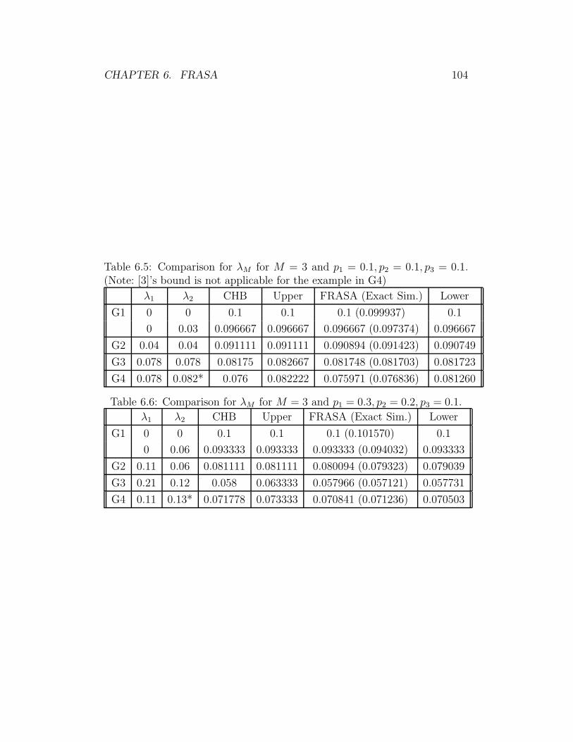
CHAPTER 6. FRASA 104
Table 6.5: Comparison for λM for M = 3 and p1 = 0.1, p2 = 0.1, p3 = 0.1.(Note: [3]’s bound is not applicable for the example in G4)
λ1 λ2 CHB Upper FRASA (Exact Sim.) Lower
G1 0 0 0.1 0.1 0.1 (0.099937) 0.1
0 0.03 0.096667 0.096667 0.096667 (0.097374) 0.096667
G2 0.04 0.04 0.091111 0.091111 0.090894 (0.091423) 0.090749
G3 0.078 0.078 0.08175 0.082667 0.081748 (0.081703) 0.081723
G4 0.078 0.082* 0.076 0.082222 0.075971 (0.076836) 0.081260
Table 6.6: Comparison for λM for M = 3 and p1 = 0.3, p2 = 0.2, p3 = 0.1.
λ1 λ2 CHB Upper FRASA (Exact Sim.) Lower
G1 0 0 0.1 0.1 0.1 (0.101570) 0.1
0 0.06 0.093333 0.093333 0.093333 (0.094032) 0.093333
G2 0.11 0.06 0.081111 0.081111 0.080094 (0.079323) 0.079039
G3 0.21 0.12 0.058 0.063333 0.057966 (0.057121) 0.057731
G4 0.11 0.13* 0.071778 0.073333 0.070841 (0.071236) 0.070503

CH
AP
TE
R6.
FR
ASA
105
Table 6.7: Comparison for λM for M = 5 and p1 = p2 = p3 = p4 = p5 = 0.5.
λ1 λ2 λ3 λ4 CHB Upper FRASA (Exact Sim.) Lower
G1 0 0 0 0 0.5 0.5 0.5 (0.499870) 0.5
0 0 0 0.015 0.485 0.485 0.485 (0.487190) 0.485
0 0 0.015 0.015 0.47 0.47 0.469521 (0.468605) 0.462021
0 0.015 0.015 0.015 0.455 0.455 0.453495 (0.455147) 0.421588
G2 0.015 0.015 0.015 0.015 0.44 0.44 0.436838 (0.433372) 0.337257
G3 0.03 0.03 0.03 0.03 0.38 0.38 0.364349 (0.347664) 0.048165
G4 0.03 0.03 0.03 0.033* 0.377 0.377 0.360352 (0.343758) 0.045835
0.033* 0.032* 0.031 0.03 0.374 0.374 0.356292 (0.330086) 0.039261
0.0325* 0.032* 0.0315* 0.03 0.374 0.374 0.356289 (0.329231) 0.037718
Table 6.8: Comparison for λM for M = 5 and p1 = 0.4, p2 = 0.5, p3 = 0.6, p4 = 0.7, p5 = 0.8.
λ1 λ2 λ3 λ4 CHB Upper FRASA (Exact Sim.) Lower
G1 0 0 0 0 0.8 0.8 0.8 (0.801848) 0.8
0 0 0 0.005 0.794286 0.78 0.78 (0.781746) 0.78
0 0 0.005 0.005 0.787619 0.76 0.759473 (0.761162) 0.744333
0 0.005 0.005 0.005 0.779619 0.74 0.738360 (0.737206) 0.685500
G2 0.002 0.003 0.005 0.005 0.779619 0.74 0.738223 (0.730949) 0.629233
G3 0.004 0.006 0.01 0.01 0.759238 0.68 0.672075 (0.664101) 0.409069
G4 0.004 0.006 0.01 0.017* 0.751238 0.652 0.640030 (0.626106) 0.172513
0.004 0.006 0.011* 0.017* 0.749905 0.648 0.635225 (0.617195) 0.152455
0.002 0.0073* 0.011* 0.017* 0.751025 0.6508 0.638890 (0.621284) 0.312233

CH
AP
TE
R6.
FR
ASA
106
Table 6.9: Comparison for λM for M = 5 and p1 = 0.77, p2 = 0.74, p3 = 0.63, p4 = 0.52, p5 = 0.51.
λ1 λ2 λ3 λ4 CHB Upper FRASA (Exact Sim.) Lower
G1 0 0 0 0 0.51 0.51 0.51 (0.513695) 0.51
0 0 0 0.0025 0.507548 0.507398 0.507398 (0.507195) 0.507398
0 0 0.003 0.0025 0.505120 0.504276 0.504259 (0.507851) 0.502567
0 0.007 0.003 0.0025 0.500295 0.496990 0.496889 (0.496086) 0.481862
G2 0.0005 0.007 0.003 0.0025 0.499964 0.496469 0.496355 (0.495522) 0.475539
G3 0.001 0.014 0.006 0.005 0.489928 0.482939 0.482467 (0.485847) 0.439008
G4 0.001 0.014 0.006 0.0057* 0.489241 0.482210 0.481704 (0.482933) 0.437699
0.001 0.014 0.0089* 0.0057* 0.486894 0.479192 0.478545 (0.476540) 0.424837
0.001 0.015* 0.0089* 0.0057* 0.486205 0.478151 0.477467 (0.479027) 0.420479
Table 6.10: Comparison for λM for M = 5 and p1 = p2 = p3 = p4 = p5 = 0.1.
λ1 λ2 λ3 λ4 CHB Upper FRASA (Exact Sim.) Lower
G1 0 0 0 0 0.1 0.1 0.1 (0.099510) 0.1
0 0 0 0.03 0.096667 0.096667 0.096667 (0.096855) 0.096667
0 0 0.03 0.03 0.093333 0.093333 0.093214 (0.092705) 0.093084
0 0.03 0.03 0.03 0.09 0.09 0.089623 (0.090675) 0.089205
G2 0.03 0.03 0.03 0.03 0.8625 0.086667 0.085870 (0.085167) 0.084971
G3 0.064 0.064 0.064 0.064 0.066685 0.071556 0.066673 (0.066963) 0.066451
G4 0.064 0.064 0.064 0.066* 0.066352 0.071333 0.066345 (0.067406) 0.066231
0.061 0.062 0.066* 0.066* 0.066852 0.071667 0.066838 (0.067879) 0.066713

CH
AP
TE
R6.
FR
ASA
107
Table 6.11: Comparison for λM for M = 5 and p1 = 0.05, p2 = 0.15, p3 = 0.2, p4 = 0.25, p5 = 0.3.
λ1 λ2 λ3 λ4 CHB Upper FRASA (Exact Sim.) Lower
G1 0 0 0 0 0.3 0.3 0.3 (0.302818) 0.3
0.008 0 0 0 0.296571 0.296571 0.296571 (0.294838) 0.296571
0.008 0.03 0 0 0.283714 0.283714 0.283559 (0.283699) 0.283324
0.008 0.03 0.04 0 0.266571 0.266571 0.265342 (0.263649) 0.263498
G2 0.008 0.03 0.04 0.06 0.241294 0.240857 0.235673 (0.236382) 0.228304
G3 0.015 0.05 0.08 0.1 0.175240 0.195 0.171271 (0.169823) 0.164827
G4 0.008 0.03 0.04 0.115* 0.212478 0.217286 0.207391 (0.207954) 0.202430
0.006 0.02 0.09* 0.115* 0.188218 0.201 0.184594 (0.183449) 0.181481

CH
AP
TE
R6.
FR
ASA
108
Table 6.12: Comparison for λM for M = 10 and p1 = p2 = p3 = p4 = p5 = p6 = p7 = p8 = p9 = p10 = 0.5.
λ1 λ2,λ3 λ4,λ5 λ6,λ7,λ8 λ9 Upper FRASA (Exact Sim.) Lower
G1 0 0 0 0 0 0.5 0.5 (0.500313) 0.5
0 0.00045 0.00045 0.00045 0.00045 0.4964 0.496389 (0.495384) 0.436516
G2 0.00045 0.00045 0.00045 0.00045 0.00045 0.49595 0.495935 (0.491676) 0.361677
G3 0.0009 0.0009 0.0009 0.0009 0.0009 0.4919 0.491840 (0.487785) 0.005261
G4 0.00097 0.00097 0.000977* 0.000977* 0.00098* 0.491225 0.491155 (0.491508) 0.002443
0.00097 0.00097 0.00097 0.000977* 0.00098* 0.491239 0.491169 (0.492485) 0.002524
Table 6.13: Comparison for λM for M = 10 and p1 = p2 = p3 = 0.1, p4 = 0.2, p5 = 0.3, p6 = 0.4, p7 = 0.5, p8 =0.6, p9 = 0.7, p10 = 0.8.
λ1 λ2, λ3 λ4 λ5 λ6 λ7 λ8 λ9 Upper FRASA (Exact Sim.) Lower
×10−3 ×10−3 ×10−3 ×10−3 ×10−3 ×10−3 ×10−3 ×10⁻³
G1 0 0 0 0 0 0 0 0 0.8 0.8 (0.801064) 0.8
0 0.15 0.35 0.5 0.5 1 2 3 0.7694 0.768940 (0.765617) 0.654316
G2 0.15 0.15 0.35 0.5 0.5 1 2 3 0.7688 0.768316 (0.768196) 0.637086
G3 0.3 0.3 0.7 1 1 2 4 6 0.7376 0.735560 (0.734688) 0.412179
G4 0.3 0.3 0.7 1 1 2 4 6.86* 0.73416 0.731926 (0.730537) 0.402376
0.01 0.327* 0.735* 1.26* 1.96* 2.94* 4.41* 6.86* 0.724684 0.721594 (0.719353) 0.041246

CH
AP
TE
R6.
FR
ASA
109
Table 6.14: Comparison for λM for M = 10 and p1 = p2 = p3 = p4 = p5 = p6 = p7 = p8 = p9 = p10 = 0.1.
λ1 λ2,λ3,λ4 λ5,λ6,λ7,λ8,λ9 Upper FRASA (Exact Sim.) Lower
G1 0 0 0 0.1 0.1 (0.099754) 0.1
0 0.019 0.019 0.083111 0.081498 (0.081612) 0.077453
G2 0.019 0.019 0.019 0.081 0.078832 (0.079277) 0.073177
G3 0.036 0.036 0.036 0.064 0.050075 (0.049960) 0.04286
G4 0.039* 0.036 0.036 0.063667 0.049130 (0.049294) 0.042554
0.039* 0.039* 0.036 0.062667 0.045913 (0.046425) 0.041415
Table 6.15: Comparison for λM for M = 10 and p1 = p2 = p3 = p4 = p5 = 0.1, p6 = p7 = p8 = p9 = p10 = 0.05.
λ1,λ2,λ3,λ4,λ5 λ6 λ7,λ8 λ9 Upper FRASA (Exact Sim.) Lower
G1 0 0 0 0 0.05 0.05 (0.049782) 0.05
0 0.01 0.01 0.01 0.047895 0.047860 (0.048058) 0.047789
G2 0.025 0.01 0.01 0.01 0.041316 0.040460 (0.040962) 0.038908
G3 0.05 0.02 0.02 0.02 0.032632 0.026879 (0.026375) 0.025804
G4 0.025 0.018 0.018 0.025* 0.039263 0.037808 (0.037468) 0.036269
0.015 0.015 0.025* 0.025* 0.041316 0.040447 (0.040123) 0.039497

Chapter 7
Conclusion and Future Works
7.1 Conclusion
The capacity of a wireless mesh network is significantly affectedby the interference among the links in the network. There-
fore, to maximize the performance of a wireless mesh networkin terms of capacity, it is crucial for wireless mesh traffic engi-neering algorithms to accurately model the interference among
the links. However, existing traffic engineering algorithms as-sumed an overly simplified binary interference model, which is
verified as an imprecise model for interference. Also, these workspresumed the existence of an ideal scheduler which can control
when each link can be active in transmission. Hence, we be-lieve there is a need to design new traffic engineering algorithmswithout assuming binary interference and perfect scheduling.
The contribution of this thesis includes the followings:
• an introduction of a new interference model: partial inter-ference, and the illustration of the potential gain in capac-
ity by exploiting partial interference;• a numerical characterization of the stability region of 802.11
networks under partial interference with two links;
• an analytical characterization of the stability region of slot-ted ALOHA networks under partial interference with two
links, and analytical results on part of the boundary of
110

CHAPTER 7. CONCLUSION AND FUTURE WORKS 111
the stability region for the case of more than two links inslotted ALOHA networks;
• an introduction of the FRASA model as a surrogate of slot-ted ALOHA to approximate the stability region of slotted
ALOHA networks, the analytical results on the stabilityregion of FRASA with any number of links under collisionchannel, binary and partial interference, and the convex
and piecewise linear outer and inner bounds on the stabil-ity region of FRASA that can be used to find upper and
lower bounds on network capacity.
7.2 Future Works
In view of this work, one of the possible future works is to con-
sider partial interference when computing the capacity of anywireless mesh network with arbitrary topology. We may modify
the interference constraints in the capacity-finding problem totake into account partial interference, and evaluate how much
will be gained by considering partial interference in schedulingin wireless networks.
Another possibility is to consider the capacity-finding prob-
lem with random access MAC protocols like 802.11 or slottedALOHA, and design traffic engineering algorithms for these net-
works. This can be used to provide QoS guarantees withoutassuming the existence of perfect global schedulers, therefore it
does not require modifying existing MAC protocols.The model in this work only covers the case of single-hop
networks. Therefore, towards designing traffic engineering al-gorithms with random access MAC protocols, we have to gen-eralize the results of this work to multi-hop wireless networks.
The stability region, the convex hull bound and the support-ing hyperplane bound obtained in this work may be used in
designing traffic engineering algorithms in wireless random ac-

CHAPTER 7. CONCLUSION AND FUTURE WORKS 112
cess networks. Extending the results on finding the maximum-hypervolume convex subset to cover the case of more than two
links helps providing a better inner bound on the stability regionof FRASA.
In this thesis, we have only considered networks with onechannel. In reality, links on different channels may also interferewith each other. Therefore, we may also extend our framework
to consider partial interference in wireless networks with multi-ple channels.
2 End of chapter.

Appendix A
Proof of (4.13) in Chapter 4
In Chapter 4, we use Pr(j1, k1|j0, k0) to denote the transitionprobability from (j0, k0) to (j1, k1). For convenience, we drop the
subscripts for τn, cn, qn, in and repeat the transition probabilitiesin (4.1)-(4.12) as follows:
Pr(j, k|j, k + 1) = 1,
j ∈ [0, m], k ∈ [0,Wj − 2], (A.1)
Pr(0, k| − 1, k + 1) = q, k ∈ [0,W0 − 2], (A.2)
Pr(−1, k| − 1, k + 1) = 1− q, k ∈ [0,W0 − 2], (A.3)
Pr(0, k|j, 0) =(1− c)qW0
,
j ∈ [0, m− 1], k ∈ [0,W0 − 1],(A.4)
Pr(−1, k|j, 0) =(1− c)(1− q)
W0,
j ∈ [0, m− 1], k ∈ [0,W0 − 1],(A.5)
Pr(0, k|m, 0) =q
W0, k ∈ [0,W0 − 1], (A.6)
Pr(−1, k|m, 0) =1− qW0
, k ∈ [0,W0 − 1], (A.7)
Pr(j, k|j − 1, 0) =c
Wj
,
j ∈ [1, m], k ∈ [0,Wj − 1], (A.8)
113

APPENDIX A. PROOF OF (4.13) IN CHAPTER 4 114
Pr(0, k| − 1, 0) =q(1− i) + q2i(1− c)
W0,
k ∈ [0,W0 − 1], (A.9)
Pr(1, k| − 1, 0) =qic
W1, k ∈ [0,W1 − 1], (A.10)
Pr(−1, k| − 1, 0) =qi(1− c)(1− q)
W0,
k ∈ [1,W0 − 1], (A.11)
Pr(−1, 0| − 1, 0) =qi(1− c)(1− q)
W0+ (1− q). (A.12)
As in Chapter 4, we use πj,k to denote the stationary prob-ability of the state (j, k) in the Markov chain. We follow the
steps listed below to solve the Markov chain and obtain thetransmission probability, i.e., (4.13).
Step 1: Express πj,k in terms of πj−1,0 for j ∈ [2, m], k ∈[0,Wj − 1]. From (A.8), we get for j ∈ [2, m],
πj,Wj−1 = πj−1,0c
Wj
.
Also for j ∈ [2, m], k ∈ [0,Wj − 2], from (A.1) and (A.8),
πj,k = πj−1,0c
Wj
+ πj,k+1
= πj,Wj−1 + πj,k+1.
Therefore, for j ∈ [2, m], k ∈ [0,Wj − 1],
πj,k = πj−1,0c(Wj − k)
Wj
. (A.13)
Step 2: Express πj,0 in terms of π1,0 for j ∈ [1, m]. From
(A.13), we obtain for j ∈ [2, m],
πj,0 = πj−1,0c.
Therefore, for j ∈ [1, m],
πj,0 = π1,0cj−1. (A.14)

APPENDIX A. PROOF OF (4.13) IN CHAPTER 4 115
Step 3: Express π1,k in terms of π−1,0 and π0,0 for k ∈[0,W1 − 1]. From (A.8) and (A.10),
π1,W1−1 = π0,0c
W1+ π−1,0
qic
W1.
Also, from (A.1), (A.8) and (A.10), for k ∈ [0,W1 − 2],
π1,k = π0,0c
W1+ π−1,0
qic
W1+ π1,k+1
= π1,W1−1 + π1,k+1.
We obtain for k ∈ [0,W1 − 1],
π1,k = π0,0c(W1 − k)
W1+ π−1,0
qic(W1 − k)W1
. (A.15)
In particular,π1,0 = π0,0c+ π−1,0qic. (A.16)
Step 4: Computem−1∑
j=0
πj,0 in terms of π0,0 and π−1,0.
From (A.14) and (A.16),
m−1∑
j=0
πj,0 = π0,0 +
m−1∑
j=1
π1,0cj−1
= π0,0 + (π0,0c+ π−1,0qic)m−1∑
j=1
cj−1
= π0,0
m−1∑
j=0
cj + π−1,0qim−1∑
j=1
cj . (A.17)
Step 5: Express π0,k in terms of π0,W0−1 for k ∈ [1,W0−2]. From (A.4), (A.6) and (A.9),
π0,W0−1 =m−1∑
j=0
πj,0(1− c)qW0
+πm,0q
W0+π−1,0
q(1− i) + q2i(1− c)W0
.

APPENDIX A. PROOF OF (4.13) IN CHAPTER 4 116
And from (A.14), (A.16) and (A.17),
π0,W0−1 = π0,0(1− cm)q
W0+ π−1,0
q2ic(1− cm−1)
W0
+(π0,0c+ π−1,0qic)cm−1q
W0+ π−1,0
q(1− i) + q2i(1− c)W0
= π0,0q
W0+ π−1,0
q2i+ q(1− i)W0
. (A.18)
From (A.1), (A.2), (A.4), (A.6) and (A.9), we obtain for k ∈[1,W0 − 2],
π0,k =m−1∑
j=0
πj,0(1− c)qW0
+ πm,0q
W0+ π−1,0
q(1− i) + q2i(1− c)W0
+π0,k+1 + π−1,k+1q
= π0,W0−1 + π0,k+1 + π−1,k+1q
Therefore, for k ∈ [1,W0 − 2],
W0−2∑
k′=k
(π0,k′ − π0,k′+1) =
W0−2∑
k′=k
(π0,W0−1 + π−1,k′+1q),
or
π0,k = π0,W0−1(W0 − k) + q
W0−2∑
k′=k
π−1,k′+1. (A.19)
Step 6: Express π−1,k in terms of π−1,W0−1 for k ∈[1,W0 − 1]. From (A.5), (A.7) and (A.11),
π−1,W0−1 =m−1∑
j=0
πj,0(1− c)(1− q)
W0
+πm,01− qW0
+ π−1,0qi(1− c)(1− q)
W0,

APPENDIX A. PROOF OF (4.13) IN CHAPTER 4 117
then from (A.14), (A.16) and (A.17),
π−1,W0−1 = π0,0(1− cm)(1− q)
W0+ π−1,0
qic(1− cm−1)(1− q)W0
+(π0,0c+ π−1,0qic)cm−1(1− q)
W0
+π−1,0qi(1− c)(1− q)
W0
= π0,01− qW0
+ π−1,0qi(1− q)W0
. (A.20)
Also, from (A.3), (A.5), (A.7) and (A.11), for k ∈ [1,W0 − 2]
π−1,k =
m−1∑
j=0
πj,0(1− c)(1− q)
W0
+πm,01− qW0
+ π−1,0qi(1− c)(1− q)
W0+ π−1,k+1(1− q)
= π−1,W0−1 + π−1,k+1(1− q).
Therefore, for k ∈ [1,W0 − 1],
π−1,k =
W0−k−1∑
k′=0
π−1,W0−1(1− q)k′
= π−1,W0−11− (1− q)W0−k
q. (A.21)
Step 7: Express π0,0 in terms of π−1,0. From (A.3), (A.5),(A.7), (A.11) and (A.12),
π−1,0 =m−1∑
j=0
πj,0(1− c)(1− q)
W0
+πm,01− qW0
+ π−1,0qi(1− c)(1− q)
W0
+π−1,1(1− q) + π−1,0(1− q)= π−1,W0−1 + π−1,1(1− q) + π−1,0(1− q)

APPENDIX A. PROOF OF (4.13) IN CHAPTER 4 118
Therefore, from (A.20) and (A.21),
π−1,0q = π−1,W0−1 + π−1,1(1− q)
= π−1,W0−1
1 +1− qq
[
1− (1− q)W0−1]
=
π0,01− qW0
+ π−1,0qi(1− q)W0
×
1 +1− qq
[
1− (1− q)W0−1]
.
On solving, we obtain
π0,0 = π−1,0q
1− qqW0 − i(1− q)
[
1− (1− q)W0
]
1− (1− q)W0
. (A.22)
Step 8: Compute the aggregate probability for stagej = −1 in terms of π−1,0. From (A.20) and (A.22),
π−1,W0−1 = π0,01− qW0
+ π−1,0qi(1− q)W0
= π−1,0
qi(1− q)W0
+1− qW0
q
1− qqW0 − i(1− q)
[
1− (1− q)W0
]
1− (1− q)W0
= π−1,0q2
1− (1− q)W0
. (A.23)
From (A.21) and (A.23),
W0−1∑
k=0
π−1,k = π−1,0 +
W0−1∑
k=1
π−1,W0−11− (1− q)W0−k
q
= π−1,0
1 +q
1− (1− q)W0
×(
W0 − 1− 1− qq
[
1− (1− q)W0−1]
)
= π−1,0qW0
1− (1− q)W0
. (A.24)

APPENDIX A. PROOF OF (4.13) IN CHAPTER 4 119
Step 9: Compute the aggregate probability for stagej = 0 in terms of π−1,0. Using (A.18), (A.19), (A.21) and
(A.23), we obtain for k ∈ [1,W0 − 2],
π0,k = π0,0q(W0 − k)
W0+ π−1,0
[q2i+ q(1− i)](W0 − k)W0
+π−1,0q2
1− (1− q)W0
W0−2∑
k′=k
[
1− (1− q)W0−k′−1]
= π0,0q(W0 − k)
W0+ π−1,0
[q2i+ q(1− i)](W0 − k)W0
+π−1,0q2
1− (1− q)W0
×
(W0 − k − 1)− 1− qq
[
1− (1− q)W0−k−1]
= π0,0q(W0 − k)
W0+ π−1,0
[q2i+ q(1− i)](W0 − k)W0
+π−1,0q2(W0 − k)− q1− (1− q)W0
+ π−1,0q(1− q)W0−k
1− (1− q)W0
. (A.25)
In (A.25), if we let k = W0 − 1, we get (A.18). If we substitutek = 0 into (A.25), we obtain (A.22), hence (A.25) holds for
k ∈ [0,W0 − 1], and,
W0−1∑
k=0
π0,k = π0,0q(W0 + 1)
2+ π−1,0
[q2i+ q(1− i)](W0 + 1)
2
+π−1,0q2W0(W0 + 1)− 2qW0
2[1− (1− q)W0]+ π−1,0(1− q)
= π−1,0
q
1− qqW0 − i(1− q)[1− (1− q)W0]
1− (1− q)W0
q(W0 + 1)
2
+[q2i+ q(1− i)](W0 + 1)
2
+q2W0(W0 + 1)− 2qW0
2[1− (1− q)W0]+ (1− q)
,
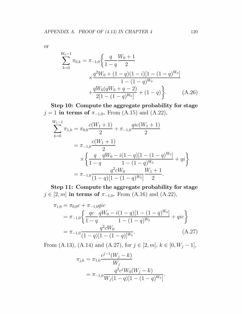
APPENDIX A. PROOF OF (4.13) IN CHAPTER 4 120
orW0−1∑
k=0
π0,k = π−1,0
q
1− qW0 + 1
2
×q2W0 + (1− q)(1− i)[1− (1− q)W0]
1− (1− q)W0
+qW0(qW0 + q − 2)
2[1− (1− q)W0]+ (1− q)
. (A.26)
Step 10: Compute the aggregate probability for stagej = 1 in terms of π−1,0. From (A.15) and (A.22),
W1−1∑
k=0
π1,k = π0,0c(W1 + 1)
2+ π−1,0
qic(W1 + 1)
2
= π−1,0c(W1 + 1)
2
×
q
1− qqW0 − i(1− q)[1− (1− q)W0]
1− (1− q)W0
+ qi
= π−1,0q2cW0
(1− q)[1− (1− q)W0]
W1 + 1
2.
Step 11: Compute the aggregate probability for stage
j ∈ [2, m] in terms of π−1,0. From (A.16) and (A.22),
π1,0 = π0,0c+ π−1,0qic
= π−1,0
qc
1− qqW0 − i(1− q)[1− (1− q)W0]
1− (1− q)W0
+ qic
= π−1,0q2cW0
(1− q)[1− (1− q)]W0
. (A.27)
From (A.13), (A.14) and (A.27), for j ∈ [2, m], k ∈ [0,Wj − 1],
πj,k = π1,0cj−1(Wj − k)
Wj
= π−1,0q2cjW0(Wj − k)
Wj(1− q)[1− (1− q)W0].

APPENDIX A. PROOF OF (4.13) IN CHAPTER 4 121
Therefore, for j ∈ [2, m],
Wj−1∑
k=0
πj,k = π−1,0q2cjW0
(1− q)[1− (1− q)W0]
Wj + 1
2. (A.28)
So (A.28) also applies to the case when j = 1.Step 12: Normalization. From (A.24), (A.26) and (A.28),
1 =
W0−1∑
k=0
π−1,k +m∑
j=0
Wj−1∑
k=0
πj,k
= π−1,0
qW0
1− (1− q)W0
+q
1− qW0 + 1
2
q2W0 + (1− q)(1− i)[1− (1− q)W0]
1− (1− q)W0
+qW0(qW0 + q − 2)
2[1− (1− q)W0]+ (1− q)
+q2W0
2(1− q)[1− (1− q)W0]
m∑
j=1
cj(Wj + 1)
.
Therefore,
π−1,0 =
qW0
1− (1− q)W0
+q
1− qW0 + 1
2
q2W0 + (1− q)(1− i)[1− (1− q)W0]
1− (1− q)W0
+qW0(qW0 + q − 2)
2[1− (1− q)W0]+ (1− q)
+q2W0
2(1− q)[1− (1− q)W0]
m∑
j=1
cj(Wj + 1)
−1
=
q2W0
2(1− q)[1− (1− q)W0]
m∑
j=0
cj(Wj + 1)
+1
2q(1− i)(W0 + 1) + (1− q)
−1
. (A.29)

APPENDIX A. PROOF OF (4.13) IN CHAPTER 4 122
Step 13: Compute the transmission probability. There-fore, from (A.14), (A.22), (A.27) and (A.29), the transmission
probability is
τ =
m∑
j=0
πj,0 + π−1,0qi
= π−1,0
qi+q
1− qqW0 − i(1− q)[1− (1− q)W0]
1− (1− q)W0
+q2cW0
(1− q)[1− (1− q)W0]
m∑
j=1
cj−1
= π−1,0q2W0
(1− q)[1− (1− q)W0]
m∑
j=0
cj
=
(
2q2W0
m∑
j=0
cj)
q2W0
m∑
j=0
cj(Wj + 1)
+(1− q)[
1− (1− q)W0
][
q(1− i)(W0 + 1) + 2(1− q)]
−1
,
which is (4.13).
2 End of chapter.

Bibliography
[1] R. Gupta, J. Musacchio, and J. Walrand, “Sufficient RateConstraints for QoS Flows in Ad-Hoc Networks,” Ad HocNetworks, 2006.
[2] R. R. Rao and A. Ephremides, “On the Stability of Inter-acting Queues in a Multiple-Access System,” IEEE Trans.
Inf. Theory, vol. 34, no. 5, pp. 918–930, Sep. 1988.
[3] W. Luo and A. Ephremides, “Stability of N Interacting
Queues in Random-Access Systems,” IEEE Trans. Inf.Theory, vol. 45, no. 5, pp. 1579–1587, Jul. 1999.
[4] P. Gupta and P. R. Kumar, “The Capacity of Wireless Net-works,” IEEE Trans. Inf. Theory, vol. 46, no. 2, pp. 388–404, Mar. 2000.
[5] K. Jain, J. Padhye, V. Padmanabhan, and L. Qiu, “Im-pact of Interference on Multi-hop Wireless Network Per-
formance,” in MobiCom 2003, San Diego, California, USA,Sep. 2003.
[6] M. Kodialam and T. Nandagopal, “Characterizing theCapacity Region in Multi-Radio Multi-Channel Wireless
Mesh Networks,” in MobiCom 2005, Cologne, Germany,Aug./Sep. 2005.
[7] J. Padhye, S. Agarwal, V. N. Padmanabhan, L. Qiu,
A. Rao, and B. Zill, “Estimation of Link Interference in
123

BIBLIOGRAPHY 124
Static Multi-hop Wireless Networks,” in Internet Measure-ment Conference, Berkeley, CA, Oct. 2005.
[8] A. Mishra, E. Rozner, S. Banerjee, and W. Arbaugh, “Ex-ploiting Partially Overlapping Channels in Wireless Net-
works: Turning a Peril into an Advantage,” in InternetMeasurement Conference, Berkeley, CA, Oct. 2005.
[9] G. Bianchi, “Performance Analysis of the IEEE 802.11 Dis-
tributed Coordination Function,” IEEE J. Sel. Areas Com-mun., vol. 18, no. 3, pp. 535–547, Mar. 2000.
[10] V. Naware, G. Mergen, and L. Tong, “Stability and Delay ofFinite-User Slotted ALOHA With Multipacket Reception,”
IEEE Trans. Inf. Theory, vol. 51, no. 7, pp. 2636–2656, Jul.2005.
[11] B. S. Tsybakov and V. A. Mikhailov, “Ergodicity of aSlotted ALOHA System,” Probl. Inform. Transm., vol. 15,no. 4, pp. 73–87, 1979.
[12] W. Szpankowski, “Stability Conditions for Multidimen-sional Queueing Systems with Computer Applications,”
Oper. Res., vol. 36, no. 6, pp. 944–957, Nov./Dec. 1988.
[13] V. Anantharam, “The Stability Region of the Finite-
User Slotted ALOHA Protocol,” IEEE Trans. Inf. Theory,vol. 37, no. 3, pp. 535–540, May 1991.
[14] W. Szpankowski, “Stability Conditions for Some Multi-queue Distributed Systems: Buffered Random Access Sys-
tems,” Adv. Appl. Probab., vol. 26, pp. 498–515, Jun. 1994.
[15] S. Ghez, S. Verdu, and S. C. Schwartz, “Stability Propertiesof Slotted Aloha With Multipacket Reception Capability,”
IEEE Trans. Autom. Control, vol. 33, no. 7, pp. 640–649,Jul. 1988.

BIBLIOGRAPHY 125
[16] S. J. Shellhammer, “Estimation of Packet Error RateCaused by Interference using Analytic Techniques - A Co-
existence Assurance Methodology,” IEEE 802.19 TechnicalAdvisory Group Document Archive, Qualcomm, Inc., Oct.
2005.
[17] T. S. Rappaport, Wireless Communications: Principles andPractice, 2nd ed. Prentice Hall, 2002.
[18] G. Mergen and L. Tong, “Stability and Capacity of Regu-lar Wireless Networks,” IEEE Trans. Inf. Theory, vol. 51,
no. 6, pp. 1938–1953, Jun. 2005.
[19] H. Wu, Y. Peng, K. Long, S. Cheng, and J. Ma, “Per-
formance of Reliable Transport Protocol over IEEE 802.11Wireless LAN: Analysis and Enhancement,” in INFOCOM
2002, Jun. 2002.
[20] Wireless LAN Medium Access Control (MAC) and PhysicalLayer (PHY) Specifications, IEEE Std. 802.11, 1999.
[21] D. Malone, K. Duffy, and D. J. Leith, “Modeling the 802.11Distributed Coordination Function in Non-saturated Het-
erogeneous Conditions,” IEEE/ACM Trans. Netw., vol. 15,no. 1, 2007.
[22] D. Kincaid and W. Cheney, Numerical Analysis: Mathe-matics of Scientific Computing, 3rd ed. Brooks/Cole, 2002.
[23] The Network Simulator - ns-2. [Online]. Available:http://www.isi.edu/nsnam/ns/
[24] R. M. Loynes, “The Stability of a Queue with Non-Independent Interarrival and Service Times,” Proc. Cam-bridge Phil. Soc., vol. 58, pp. 494–520, 1962.

BIBLIOGRAPHY 126
[25] S. S. Lam, “Store-and-Forward Buffer Requirements ina Packet Switching Network,” IEEE Trans. Commun.,
vol. 24, no. 4, Apr. 1976.
[26] J. R. Wieland, R. Pasupathy, and B. W. Schmeiser,
“Queueing-Network Stability: Simulation-Based Check-ing,” in Proceedings of the 2003 Winter Simulation Con-ference, vol. 1, Dec. 2003, pp. 520–527.
[27] J.-S. Chang and C.-K. Yap, “A Polynomial Solution forPotato-Peeling and Other Polygon Inclusion and Enclosure
Problems,” in 25th Annual Symposium on Foundations ofComputer Science, Oct. 1984, pp. 408–416.