characterization of municipal waste waters
TRANSCRIPT

Univers
ity of
Cap
e Tow
n
CHARACTERIZATION OF MUNICIPAL
W ASTEW ATERS
by
Alfred Mbewe
BSc (Eng) (Malawi), R Eng (Malawi)
Thesis submitted in partial fulfilment of the
requirements for the degree of Master of Science in
Engineering at the University of Cape Town.
Department of Civil Engineering
University of Cape Town September 1995

The copyright of this thesis vests in the author. No quotation from it or information derived from it is to be published without full acknowledgement of the source. The thesis is to be used for private study or non-commercial research purposes only.
Published by the University of Cape Town (UCT) in terms of the non-exclusive license granted to UCT by the author.
Univers
ity of
Cap
e Tow
n
DECLARATION BY CANDIDATE
I, ALFRED MBEWE, hereby declare that this thesis is
my own work and has not been submitted at another
University.
28 September 1995

SYNOPSIS
BACKGROUND AND OBJECTIVES
Over the past 20 years there have been extensive developments in the activated
sludge method of treating wastewater. The functions of the single sludge system
have expanded from carbonaceous energy removal to include progressively
nitrification, denitrification and phosphorus removal, all mediated biologically. Not
only has the system configuration and its operation increased in complexity, but
concomitantly the number of biological processes influencing the system performance
and the number of compounds involved in these processes have increased. With
such complexity, designs based on experience or semi-empirical methods no longer
will give optimal performance; design procedures based on more fundamental
behavioural patterns are required. Also, it is no longer possible to make a reliable
quantitative, or sometimes even qualitative prediction as to the effluent quality to
be expected from a design, or to assess the effect of a system or operational
modification, without some model that simulates the system behaviour accurately.
To address these problems, over a number of years design procedures and kinetic
models of increasing complexity have been developed, to progressively include
aerobic COD removal and nitrification (Marais and Ekama, 1976; Dold et al., 1980),
anoxic denitrification ( van Haandel et al., 1981; WRC, 1984; Henze et al., 1987;
Dold et al., 1991) and anaerobic, anoxic, aerobic biological excess phosphorus
removal (Wentzel et al., 1990; ·wentzel et al., 1992; Henze et al., 1995).
In terms of the framework of these design procedures and kinetic models, the
influent carbonaceous (C) material (measured in terms of the COD parameter) is
subdivided into a number of fractions - this subdivision is specific to the structure
of this group of models. The influent COD is subdivided into three main fractions,
biodegradable, unbiodegradable and heterotrophic active biomass. The
unbiodegradable COD is subdivided into particulate and soluble fractions based on
whether the material will settle out in the settling tank (unbiodegradable
particulate) or not (unbiodegradable soluble). The biodegradable material also has
two subdivisions, slowly biodegradable (SB COD) and readily biodegradable
(RBCOD); this subdivision is based wholly on the dynamic response observed in
aerobic (Dold et al., 1980) and anoxic/aerobic (van Haandel et al., 1981) activated
sludge systems, that is, the division is biokinetically based. Thus, as input to the
design procedures and kinetic models, it is necessary to quantify five influent COD
fractions, that is, to characterize the wastewater COD. From a review of the
11
literature on existing tests to quantify the COD fractions, it was evident that the
existing procedures are either too elaborate or approximate or sometimes not even
available. This research project addresses these deficiencies.
In this research project, the principal objective was to develop simple accurate
procedures to quantify the influent wastewater COD fractions. A batch test method
has been developed to quantify the five influent COD fractions; namely
heterotrophic active biomass, readily biodegradable COD, slowly biodegradable
COD, unbiodegradable particulate COD and unbiodegradable soluble COD. Also,
the physical flocculation-filtration method of Mamais et al. (1993) to quantify
RBCOD has been evaluated and refined.
BATCH TEST
In the batch test, the influent wastewater to be tested is placed in a stirred batch
reactor, aerated and the oxygen utilization rate (OUR) monitored automatically
with time (Randall et al., 1991). Also, samples are drawn from the start and end of
the test and total COD and nitrate concentrations determined. From these data the
following can be calculated:
• COD recovery (%)
• Wastewater heterotrophic active biomass, Zntt< ol (mgCOD/t)
• Wastewater RBCOD, Sbsi (mgCOD/t)
• Wastewater heterotrophic maximum specific growth rate on RBCOD, JLH (/d)
• Wastewater heterotrophic maximum specific growth rate on SBCOD, KMP (/d)
Using raw (unsettled) municipal wastewater from two sources (Borcherds Quarry
and Mitchell's Plain, Cape Town, South Africa) the batch test procedure was
comprehensively evaluated. Results for RBCOD from the batch test were compared
to those from the conventional square-wave flow through activated sludge system
method (Ekama and Marais, 1979; \VRC, 1984; Ekama et al., 1986). The results
indicated that:
• COD recoveries in the batch test are generally good, the majority falling in the
range 95-105% indicating the reliability of the method.
• For wastewaters from both Borcherds Quarry and Mitchell's Plain autotrophic
active biomass could not be detected in the batch test, indicated by an absence
lll
of nitrification (no increase in nitrate concentration).
• For Mitchell's Plain wastewater, usually heterotrophic active biomass was
present in low concentrations, ranging from 3% to 10% of total COD. However,
on occasion concentrations > 10% of total COD were measured. These high
values could be traced to operational procedures at the Mitchell's Plain
Wastewater Treatment Plant - sludge handling facilities were shut down for
maintenance and repairs and waste sludge recycled to the head of the works
upstream of the point where the wastewater was collected for the batch tests.
• For Borcherds Quarry wastewater, heterotrophic active biomass concentration
was very variable, ranging from 7% to 16% of total COD. From an investigation
of operational procedures at the Borcherds Quarry Wastewater Treatment Plant,
it was found that intermittently waste activated sludge was recycled to the head
of the works and mixed with the incoming wastewater upstream of the point
where wastewater was drawn for the batch test.
• Although the heterotrophic active biomass concentration obtained from the batch
test could not be compared to a conventional test (no such test was available),
the values measured in the batch test could correctly reflect changes arising from
Wastewater Treatment Plant operation.
• The values for the kinetic constants derived from the batch test (KMP and iitt) differ from those in literature for activated sludge. Most probably a population
develops in the activated sludge system (low COD, high active mass) that differs
appreciably from that in the wastewater (high COD, low active mass).
Accordingly it is unlikely that the values for the constants derived from the
batch test ( which reflect the wastewater population) will be of much value in
modelling and design of activated sludge systems - their use is restricted to the
batch test to derive estimates for RBCOD.
The batch test was extended to quantify soluble unbiodegradable COD. This
extension was achieved by drawing a sample from the batch reactor at the end of
the test, flocculating with aluminium sulphate and filtering through 0,45µm filter
paper; the COD of the filtrate gives the unbiodegradable soluble COD (USCOD).
To evaluate this extension, results from the batch test were compared to those from
the effluent of a long sludge age activated sludge system (Ekama et al., 1986).

lV
Results indicated that:
• The batch test method gives values for USCOD that tend to be slightly higher
than those from the activated sludge system methods; this may be due to the
inability of the organisms within the batch test to degrade some of the soluble
biodegradable material. However, the differences in USCOD between the two
methods are relatively small ( < 10%) - the estimates provided by the batch tests
are acceptable for design and modelling purposes. Furthermore, values for
USCOD as a fraction of the total COD from the batch test (fus = 0,07 to 0,10)
fall within the range of values to be expected for a South African raw municipal
wastewater (fus = 0,04 to 0,10; WRC, 1984).
• Glass fibre filters can replace the 0,45µm filters without any loss in accuracy.
Having developed the batch test method to quantify three of the five influent COD
fractions, namely RBCOD, heterotrophic active biomass and USCOD, various
extensions to the batch test to provide estimates for unbiodegradable particulate
COD and slowly biodegradable COD were proposed and evaluated:
• Division of OUR.
• Pasteurization of influent.
• Extended aeration.
• OUR at the end of batch test.
• Addition of acetate.
• Addition of flocculated-filtered raw sewage.
Of all the proposals above, only the last ( namely addition of flocculated-filtered raw
sewage) appeared to hold promise for development. In this proposed method, raw
wastewater is flocculated with aluminium sulphate and filtered through 0,45µm filter
papers. The filtrate is added to the batch test after about 2days. From the
exponential increase in OUR after sewage filtrate addition, the heterotrophic active
biomass concentration in the batch test at the time of adding the sewage filtrate can
be determined from which the remaining two COD fractions can be quantified (i.e.
slowly biodegradable and unbiodegradable particulate COD). This method was
evaluated by comparing estimates for unbiodegradable particulate COD and slowly
biodegradable COD with those from the conventional activated sludge method
(Ekama et al., 1986).

V
Although the proposed extension to the batch test method to determine influent
slowly biodegradable (Sbpi) and unbiodegradable particulate (Supi) COD provides
estimates for Sbpi and Supi that fall in the same range as estimates from the
conventional completely aerobic activated sludge system method (Ekama et al.,
1986), the direct correlation between the estimates from the two methods is poor.
The batch test method provides estimates for Supi that tend to be higher than those
derived from the conventional activated sludge method and correspondingly provides
estimates for Sbpi that tend to be lower than those derived from the conventional
activated sludge method. A more extensive experimental evaluation is required to
discern if these trends are consistent.
FLOCCULATION-FILTRATION METHOD
A flocculation-filtration method has been developed by Mamais et al. (1993) to
quantify the influent RBCOD concentration. In this method, the inclusion of the
flocculation step prior to filtration appears to overcome the problem of correct
selection of filter pore size inherent in other physical methods. In the Mamais et al.
method, raw wastewater is flocculated using zinc sulphate with the pH adjusted to
10,5. The flocculated wastewater is then filtered through 0,45µm filter paper.
Likewise effluent from an activated sludge system is also flocculated and then
filtered through 0,45µm filter papers. The difference between the COD of the
filtrates of the raw wastewater and the effluent gives the RBCOD concentration.
In preliminary tests it was found that the zinc sulphate flocculant recommended by
Mamais et al. could be replaced with aluminium sulphate - this has the advantage
that no pH adjustment is necessary. The physical flocculation-filtration method
was evaluated by comparing the RBCOD concentration measured with this method
with those from the batch test and "standard" flow-through square wave methods.
Also, the experimental protocol was examined to determine whether this could be
improved by using glass fibre filter papers in place of the expensive 0,45µm filter
papers. Results showed that the flocculation-filtration method provided estimates
that correlated closely with those from both the batch test and the flow-through
square wave methods and that the 0,45µm filter paper can be replaced with glass
fibre filter paper to reduce the cost of this method without any loss in accuracy.

Vl
CONCLUSIONS The batch test method developed in this investigation has advantages over previous
methods in that,
• The experimental ~,rocedure is relatively simple.
• No mixed liquor acclimatized to the wastewater is required.
• The only independent constants required for calculation are the heterotrophic
yield (Y ztt), endogenous residue fraction for heterotrophic active biomass (f), and
specific death rate (bH): Dosing the batch test with known concentrations of
acetate showed that the standard value for Y zH in the literature (Y ZH = 0,666
mgCOD/mgCOD; Dold and Marais, 1986) can be accepted; the batch test
procedure is relatively insensitive to the value for bH. All other constants
required for calculations are obtained from the experimental data. However, it is
unlikely that these constants (i.e. maximum specific growth rate of heterotrophs
on RBCOD, ILH, and maximum specific growth rate of heterotrophs on SBCOD,
KMP) will be of much value in modelling and design of activated sludge systems -
most probably a population will develop in the activated sludge system that
differs appreciably from that in the wastewater since the conditions in the
wastewater (high COD, low active mass) differ significantly from those in the
activated sludge system (low COD, high active mass).
The batch test method was evaluated by comparing its results with those from
conventional flow through activated sludge system methods accepted as the
standard in the literature. Results from a number of batch tests on municipal
wastewater from l\'litchell's Plain and Borcherds Quarry ( Cape Town, South Africa)
indicate that:
• Autotrophic biomass is not present in either wastewater.
• Measured RBCOD concentrations correlate closely with those from the
conventional square-wave flow through method (WRC, 1984; Ekama et al.,
1986).
Vll
• Although the values for wastewater heterotrophic active biomass could not be
compared to conventional methods (none are available), the batch test was able
to detect correctly variations in heterotrophic active biomass caused by changes
in plant operational procedures, as described above.
• Values for unbiodegradable soluble COD derived from the batch test compared
reasonably well with those derived from the effluent of a long sludge age
activated sludge system (Ekama et al., 1986).
• Values for unbiodegradable particulate COD derived from the batch test fall in
the same range as estimates from the conventional completely aerobic activated
sludge system method (Ekama et al., 1986). However, the direct correlation
between the values from the two tests is poor. For the present, the batch test
does not provide estimates for unbiodegradable particulate COD that are
sufficiently accurate and precise for use in design and simulation of activated
sludge systems. For design and simulation, unbiodegradable particulate COD as
a fraction of total COD should at least be able to be quantified into the ranges
0-0,05; 0,05-0,10; 0,10-0,15; etc. As yet, there is not sufficient surety that the
estimate for fup from the batch test will meet this requirement; more data are
required.
• The errors in unbiodegradable particulate COD are reflected in the estimate from
the batch test for ·slowly biodegradable COD. However, because the absolute
value for the slowly biodegradable COD concentration is very much larger than
that for the unbiodegradable particulate COD concentration, the relative error in
the estimate for slowly biodegradable COD is very much less. The estimate for
slowly biodegradable COD can be accepted for design and simulation.
For the flocculation-filtration method proposed by Mamais et al. (1993) to
determine RBCOD:
• The zinc sulphate flocculant recommended by Mamais et al. (1993) can be
replaced with aluminium sulphate. This has the advantage that pH adjustment
after flocculation is now required.

Vlll
• Measured RBCOD correlate closely with those from the conventional
flow-through square wave method (WRC, 1984; Ekama et al., 1986) and the
batch test method.
• The method is relatively simple and easy to apply but requires independent
determination of unbiodegradable soluble COD, from effluent samples which may
not always be available.
• The 0,45µm filters recommended by Mamais et al. ( 1993) can be replaced with
glass fibre filters (Whatman's GF /C) to reduce costs, without any loss in
accuracy.
RECOMMENDATIONS
From this investigation, the following recommendations can be made:
• The batch test can be used successfully to determine the heterotrophic active
biomass, RBCOD and the soluble unbiodegradable COD concentrations in the
influent wastewater. In this investigation, the estimates for RBCOD and
unbiodegradable soluble COD concentrations from the batch test could be
compared to results from conventional test methods. However, the heterotrophic
active biomass concentration could not be evaluated against other tests because
no such tests are available. To evaluate estimates for heterotrophic active
biomass, it is recommended that an inoculum of activated sludge mixed liquor
from a defined continuous flow steady state system is introduced into the batch
test. From the steady state model (\VRC, 1984) the concentration of the
heterotrophic active biomass in the continuous flow system and therefore added
into the batch test can be calculated, and compared to the concentration
obtained from the batch test. However, due account must be taken of
nitrification, since the mixed liquor dosed to the batch test may nitrify. If
similar results are obtained then a powerful verification of the basis of present
activated sludge models ( see Background and Objectives above) will have been
provided.
• For the batch test method, a technique has been developed to quantify the
unbiodegradable particulate COD and slowly biodegradable COD fractions.
However, direct correlation of estimates for these parameters from the batch test
and conventional tests were poor. Also, no discernible trends could be identified

IX
in the relationship between values from the two tests. To identify clear trends, a
more extensive experimental investigation is required, so that more data are
available.
• This investigation has been restricted to quantifying the influent carbonaceous
material fractions. Similar studies should be undertaken on the influent
nitrogenous and phosphorous materials.

X
ACKNOWLEDGEMENTS
I wish to express my sincere gratitude and appreciation to the following persons for their contribution during the time of the laboratory investigation and up to the time of writing up this thesis:
• Dr M C Wentzel - for his untiring and relentless guidance during the experimental investigations and writing up.
• Professors G A Ekama and GvR Marais - for their support, tips and interest throughout the time of the experimental investigation and writing up.
• Mr T Lakay - for his invaluable help in showing and helping me to run the units and the experimental work.
• Mrs Heather Bain - for so cheerfully typing ( and retyping) this thesis.
• Messrs James George, Douglas Swartz - for keeping the experimental equipment clean and helping with the daily experimental work in the laboratory.
• Dr N J Marais - for developing and supplying the spreadsheet programme for the statistical plots.
Thanks to Van Wyk and Louw Inc. (Pretoria) for the financial support accorded to me in the second year of my studies and the Water Research Commission for funding the whole research.

xi
TABLE OF CONTENTS
SYNOPSIS
ACKNOWLEDGEMENTS
TABLE OF CONTENTS
LIST OF FIGURES
LIST OF TABLES
LIST OF SYMBOLS
CHAPTER 1: INTRODUCTION
CHAPTER 2: WASTEWATER CHARACTERIZATION FOR ACTIVATED SLUDGE SYSTEM 2.1 Introduction 2.2 Wastewater characterization for the activated sludge
system 2.3 Carbonaceous materials
2.3.1 Carbonaceous material (COD) fractions 2.3.2 Analytical formulation {or COD 2.3.3 Typical wastewater COD fractions
2.4 Factors influencing wastewater characteristics 2.4.1 Input to the sewer 2.4.2 Transformation in the sewer 2.4.3 Physical/chemical treatment prior to activated
sludge system 2.5 Closure Figures Table
CHAPTER 3: EXISTING METHODS FOR QUANTIFICATION OF WASTEWATER COD FRACTIONS 3.1 Introduction 3.2 Quantification methods
3.2.l Readily biodegradable COD (RBCOD) measurement 3.2.2 RBCOD subfractions 3.2.3 Influent heterotrophic active biomass measurement 3.2.4 Unbiodegradable soluble COD measurement 3.2.5 Unbiodegradable particulate and slowly
biodegradable CODs measurement 3.3 Conclusion Figures
CHAPTER 4: BATCH TEST FOR MEASUREMENT OF READILY BIODEGRADABLE COD AND ACTIVE ORGANISM CONCENTRATION IN MUNICIPAL WASTEWATER 4.1 Introduction 4.2 Test procedure 4.3 Results
Page
i
X
xi
xv
xxi
XXlll
1.1
2.1
2.2 2.4 2.4 2.8
2.11 2.12 2.12 2.13
2.13 2.14 2.15 2.18
3.1 3.1 3.1
3.12 3.12 3.13
3.14 3.15 3.16
4.1 4.1 4.2
xii
4.4 Data interpretation 4.2 4.4.1 COD recovery 4.3 4.4.2 Wastewater heterotroph active biomass 4.4 4.4.3 Heterotroph maximum specific growth rate on SBCOD 4.6 4.4.4 Heterotroph maximum specific growth rate on RBCOD 4.8 4.4.5 Determination of influent RBCOD fraction 4.8
4.5 Closure 4.10 Figures 4.11 Table 4.12
CHAPTER 5: EVALUATION OF BATCH TEST FOR MEASUREMENT OF READILY BIODEGRADABLE COD AND ACTIVE ORGANISM CONCENTRATION 5.1 Introduction 5.1 5.2 Method 5.1 5.3 Results 5.2
5.3.1 COD recovery 5.2 5.3.2 Wastewater autotrophic biomass concentration 5.3 5.3.3 Heterotrophic active biomass 5.3 5.3.4 Heterotroph maximum specific growth rates on
RBCOD and SBCOD 5.5 5.3.5 Wastewater RBCOD concentration 5.6
5.4 Conclusions 5. 7 Figures 5.9 Tables 5.23
CHAPTER 6: EVALUATION OF A PHYSICAL FLOCCULATIONFILTRATION METHOD TO DETERMINE RBCOD 6.1 Introduction 6.1 6.2 Test procedure 6.1 6.3 Results 6.3 6.4 Conclusions 6.4 Figures 6.6 Tables 6.10
CHAPTER 7: EXTENSION OF THE BATCH TEST TO DETERMINE UNBIODEGRADABLE SOLUBLE COD 7.1 Introduction 7.1 7.2 Test procedure 7.2 7.3 Results 7.2 7.4 Conclusions 7.3 Figures 7.4 Table 7.8
CHAPTER 8: EXTENSION OF BATCH TEST TO DETERMINE UNBIODEGRADABLE PARTICULATE AND SLOWLY BIODEGRADABLE COD FRACTIONS 8.1 Introduction 8.1 8.2 Background 8.1 8.3 METHOD 1: Division of OUR area 8.3
8.3.1 Test procedure 8.4 8.3.2 Data interpretation 8.4 8.3.3 Results 8.5 8.3.4 Conclusions 8.6

xiii
8.4 METHOD 2: Pasteurization of sewage 8.4.1 Test procedure 8.4. 2 Results 8.4.3 Conclusions
8.5 METHOD 3: Extended aeration 8.5.1 Test procedure 8.5.2 Data interpretation 8.5.3 Results 8.5.4 Conclusions
8.6 METHOD 4: OUR at end of batch test 8.6.1 Test procedure 8.6.2 Data interpretation 8.6.3 Results 8.6.4 Conclusions
8. 7 METHOD 5: Acetate addition 8. 7 .1 Biomass behaviour with acetate addition
- preliminary investigation 8. 7.2 Test procedure 8.7.3 Data evaluation 8. 7.4 Results 8.7.5 Conclusions
8.8 METHOD 6: Raw sewage filtrate addition 8.8.1 Test procedure 8.8.2 Data interpretation 8.8.3 Improvements to test procedure 8.8.4 Results 8.8.5 Conclusions
8.9 Conclusions Figures Tables
CHAPTER 9: EVALUATION OF BATCH TEST EXTENSION TO DETERMINE UNBIODEGRADABLE PARTICULATE COD 9.1 Introduction 9.2 Method 9.3 Comparative analysis of results 9.4 Conclusions Figures Table
CHAPTER 10: CONCLUSION 10.1 Objectives 10.2 Batch test method 10.3 Flocculation-filtration method 10.4 Recommendations
REFERENCES
APPENDIX A: OUR-TIME PLOTS FOR THE BATCH TESTS
APPENDIX B: COMPREHENSIVE DATA FOR THE BATCH TESTS
APPENDIX C: CONSTRUCTION AND INTERPRETATION OF STATISTICAL PLOTS FOR DATA ANALYSIS
8.6 8.8 8.8 8.8 8.9 8.9 8.9
8.10 8.11 8.11 8.11 8.12 8.13 8.14 8.14
8.15 8.16 8.16 8.18 8.19 8.19 8.20 8.20 8.21 8.22 8.23 8.23 8.24 8.35
9.1 9.1 9.4 9.6 9.7 9.9
10.1 10.2 10.4 10.4
R.l

XIV
APPENDIX D: COMPLETELY AEROBIC ACTIVATED SLUDGE SYSTEM
APPENDIX E: COMPREHENSIVE DATA FOR THE FLOCCULATION-FILTRATION METHOD TO DETERMINE RBCOD
APPENDIX F: COMPARISON OF RBCOD DATA FROM THE. BATCH TEST, FLOW-THROUGH SQUARE WAVE AND FLOCCULATION-FILTRATION METHODS
APPENDIX G: DATA ON UNBIODEGRADABLE SOLUBLE COD FROM BATCH TEST AND ACTIVATED SLUDGE SYSTEM EFFLUENT
APPENDIX H: PROCEDURE FOR THE BATCH TEST METHOD

Page No.
2.15 Fig 2.1:
2.16 Fig 2.2:
2.17 Fig 2.3:
3.16 Fig 3.1:
3.16 Fig 3.2:
3.17 Fig 3.3:
3.17 Fig 3.4:
3.18 Fig 3.5:
3.19 Fig 3.6:
3.19 Fig 3.7:
3.20 Fig 3.8:
3.21 Fig 3.9:
4.11 Fig 4.1:
xv
LIST OF FIGURES
Division of influent wastewater carbon (C), nitrogen (N) and phosphorus (P) materials according to the biological and physical processes in the activated sludge system.
The general wastewater characterization structure for carbon (C), nitrogen (N) and phosphorus (P) material.
The division of COD into its different constituents.
Molecular weight distribution of dissolved organic carbon (DOC) in the influent and effluent of laboratory activated sludge system treating a mixture of glucose and glutamic acid. (After Leidner et al., 1984).
Molecular weight distribution of dissolved organic carbon (DOC) in the cell-free extract of sludge in a laboratory activated sludge system treating a mixture of glucose and glutamic acid. (After Leidner et al., 1984 ).
Examples of daily data pairs for a number of sewage batches, values of readily biodegradable COD (Sbs) determined by ultra-filtration plotted versus values obtained by the flow-through square wave method. (After Dold et al., 1986).
COD of raw wastewater 0,45µm filtrate plotted versus corresponding values of the readily biodegradable COD (Sbs) obtained bf the flow-through square wave method. (After Dold et al., 1986 ).
OUR response over one cycle in an aerobic activated sludge unit subjected to daily cyclic square wave feed (12h feed on, 12h feed off) with municipal wastewater as influent. (After Ekama et al., 1986).
OUR-time profile for aerobic batch test with activated sludge addition, with nitrification. (After Dold et al., 1991).
OUR-time profile for aerobic batch test to show the effect of loading rate on the shape of the OUR-time plot. (After Dold et al., 1991).
Example of nitrate concentration-time plot in an anoxic batch test for measuring the influent readily biodegradable COD concentration. (After Ekama et al., 1986).
Schematic representation of the transformations of the influent COD fractions within the activated sludge system.
OUR-time plot for aerobic batch test on raw municipal wastewater from Mitchell's Plain Treatment Plant.

Page No.
4.11 Fig 4.2:
5. 9 Fig 5.la:
5.10 Fig 5.lb:
5.11 Fig 5.2a:
5.12 Fig 5.2b:
5.13 Fig 5.3:
5.13 Fig 5.4:
5.14 Fig 5.5:
5.14 Fig 5.6:
5.15 Fig 5.7:
5.15 Fig 5.8:
5.16 Fig 5.9:
5.16 Fig 5.10:
5.17 Fig 5.11:
xvi
tn-OUR versus time for the measured OUR data in Fig 4.1 up to the precipitous drop in OUR.
OUR-time plot for aerobic batch test on raw municipal wastewater from Borcherds Quarry Treatment Plant.
tn-OUR versus time for the measured OUR data in Fig 5.la up to the precipitous drop in OUR.
OUR-time plot for aerobic batch test on raw municipal wastewater from Mitchell's Plain Treatment Plant.
tn-OUR versus time for the measured OUR data in Fig 5.2a up to the precipitous drop in OUR.
Probability plot of % COD recovery from the batch test results for wastewater from Borcherds Quarry Treatment Plant.
Probability plot of % COD from the batch test results for wastewater from Mitchell's Plain Treatment Plant.
Probability plot of heterotroph active biomass COD (as a % of total wastewater COD concentration) from the batch test results on a batch of wastewater from Borcherds Quarry Treatment Plant. (Sewage batch No. 1).
Probability plot of heterotroph active biomass COD (as a % of total wastewater COD concentration) from the batch test results on a batch of wastewater from Mitchell's Plain Treatment Plant. (Sewage batch No. 20).
Probability plot of the means of heterotroph active biomass (%) for the different wastewater batches from Borcherds Quarry Treatment Plant.
Probability plot of the means of heterotroph active biomass (%) for the different wastewater batches from Mitchell's Plain Treatment Plant.
Probability plot of heterotroph maximum specific growth rate on SBC OD (KMP) for batch tests on one wastewater batch from Borcherds Quarry Treatment Plant. (Sewage batch No.8).
Probability plot of heterotroph maximum specific growth rate on SBC OD (KMP) for batch tests on one wastewater batch from Mitchell's Plain Treatment Plant. (Sewage batch No.17).
Probability plot of the means of heterotroph maximum specific growth rate on SBCOD (KMP) for the different wastewater batches from Borcherds Quarry Treatment Plant.

5.17 Fig 5.12:
5.18 Fig 5.13:
5.18 Fig 5.14:
5.19 Fig 5.15:
5.19 Fig 5.16:
5.20 Fig 5.17a:
5.20 Fig 5.17b:
5.21 Fig 5.18a:
5.21 Fig 5.18b:
5.22 Fig 5.19:
6. 6 Fig 6.1:
6. 6 Fig 6.2:
6. 7 Fig 6.3:
XVll
Probability plot of the means of heterotroph maximum specific growth rate on SBC OD (KMP) ·for the different wastewater batches from Mitchell's Plain Treatment Plant.
Probability plot of heterotrophic maximum specific growth rate on RBCOD (µH) for batch tests on one wastewater batch from Borcherds Quarry Treatment Plant. (Sewage batch No.8).
Probabilit(j plot of heterotroph maximum specific growth rate on RBCOD µH) for batch tests on one batch of wastewater from Mitchell's Plain Treatment Plant. (Sewage batch No.17).
Probability plot of the means of heterotrophic maximum specific rowth rate on RBCOD (µH) for the different wastewater batches rom Borcherds Quarry Treatment Plant.
Probability plot of the means of heterotrophic maximum specific rirowth rate on RBCOD (µH) for the different wastewater batches rom Mitchell's Plain Treatment Plant.
Probability plot of RBCOD (% of total COD, Sti) derived from the batch test for one batch of wastewater from Borcherds Quarry Treatment Plant. (Sewage batch No.8).
Probability plot of RBCOD (% of total COD, Sti) derived from the flow-through square wave test for one batch of wastewater from Borcherds Quarry Treatment Plant (Sewage batch No.8).
Probability plot of RBCOD (% of total COD, Sti) derived from the batch test for one batch of wastewater from Mitchell's Plain Treatment Plant. (Sewage batch No.10).
Probability plot of RBCOD (% of total COD, Sti) derived from the flow-through square wave test for one batch of wastewater from Mitchell's Plain Treatment Plant. (Sewage batch No.10).
Readily biodegradable COD (RBCOD, as % of total COD) derived from the batch test versus those from the flow-through square wave method. Each data point is the mean of a number of tests on one batch of sewage.
Probability plot of RBCOD (% of total COD, Sti) derived from the 0,45µm flocculation-filtration test for one batch of sewage from Borcherds Quarry Treatment Plant. (Sewage batch No.9).
Probability plot of RBCOD (% of total COD, Sti) derived from the glass fibre flocculation-filtration test for one batch of sewage from Borcherds Quarry Treatment Plant. (Sewage batch No.9).
Probability plot of RBCOD (% of total COD, Sti) derived from the flow-through square wave test for one batch of sewage from Borcherds Quarry Treatment Plant. (Sewage batch No.9).

6. 7 Fig 6.4:
6. 8 Fig 6.5:
6. 8 Fig 6.6:
6. 9 Fig 6.7:
6. 9 Fig 6.8:
7. 4 Fig 7.1:
7. 4 Fig 7.2:
7. 5 Fig 7.3:
7. 5 Fig 7.4:
7. 6 Fig 7.5:
7. 6 Fig 7.6:
7. 7 Fig 7.7:
8.24 Fig 8.1:
xviii
Probability plot of RBCOD (% of total COD, Sti) derived from the batch wave test for one batch of sewage from Borcherds Quarry Treatment Plant. (Sewage batch No.9).
RBCOD derived from the 0,45µm flocculation-filtration test versus those from the flow-through square wave test. Each data point is the mean of a number of tests on one batch of sewage.
COD concentration following flocculation-filtration through glass fibre filters versus those following flocculation-filtration through 0,45µm filters. Both influent and effluent samples are plotted.
RBCOD derived from the glass fibre flocculation-filtration test versus those from 0,45µm flocculation-filtration test. Each data point is the mean of a number of tests on one batch of sewage.
RBCOD derived from 0,45µm flocculation-filtration test versus those from the batch test. Each data point is the mean of a number of tests on one batch of sewage.
Unbiodegradable soluble COD concentrations determined from the batch test versus those determined from the effluent of a laboratory-scale completely aerobic activated sludge unit operated at a sludge age of 12 days. Each data point is single measurement.
Duplicate plot of Fig 7.1 with axes extended to 500 mgCOD/l, the approximate total COD concentration of the sewage in the tests.
Data in Fig 7.1 plotted as % of the total COD (Sti).
Unbiodegradable soluble COD concentrations derived from the batch test using 0,45µm filtration versus those using glass fibre filtration.
Probability plot of soluble unbiodegradable COD for batch tests on one batch of sewage from Mitchell's Plain Treatment Plant. (Sewage batch No.22).
Probability plot of the soluble unbiodegradable COD derived from the aerobic unit effluent for one batch of sewage from Mitchell's Plain Treatment Plant. (Sewage batch No.22).
Soluble unbiodegradable COD from the batch test versus that from the aerobic unit. Each data point is the mean of a number of tests on one batch of sewage.
OUR-time plot for an aerobic batch test run for an extended period showing the division of the area under the OUR graph according to METHOD 1.

8.25 Fig 8.2:
8.26 Fig 8.3:
8.27 Fig 8.4:
8.28 Fig 8.5:
8.28 Fig 8.6:
8.29 Fig 8. 7a:
8.29 Fig 8.7b:
8.30 Fig 8.7c:
8.31 Fig 8.8a
8.31 Fig 8.8b:
8.32 Fig 8.9a:
8.32 Fig 8.9b:
XIX
BOD, bacteria and protozoa counts during a WARBURG study with non-pasteurized sewage seed used for the BOD test determination. (From Bhatla et al., 1965). .
BOD and bacteria count during a WARBURG study with pasteurized sewage seed used for the BOD test determination. (From Bhatla et al., 1965).
OUR-time plot for an aerobic batch test with pasteurized sewage.
OUR-time plot for an aerobic batch test run for an extended period showing the division of the OUR area into the different OUR uptakes for the various COD utilizations.
Theoretical variation of unbiodegradable particulate COD fraction (fu:e) with variation in the absolute value of the OUR at the end of the batch test (Oee)-
OUR-time plot for an aerobic batch test with acetate added after the precipitous drop in OUR, to determine the yield coefficient with acetate as substrate.
OUR-time plot for an aerobic batch test with acetate added at the end of the batch test to stimulate exponential heterotroph growth due to the utilization of the acetate RBCOD.
OUR-time plot for an aerobic batch test with acetate added at the end of the batch test to stimulate exponential heterotroph growth due to the utilization of the acetate RBCOD.
OUR-time plot for an aerobic batch test with raw sewage filtrate (0,45µm) added at the end of the batch test to stimulate exponential heterotroph growth due to the utilization of the filtrate RBCOD.
OUR-time plot for an aerobic batch test with flocculated-filtered (0,45µm) raw sewage filtrate added at the end of the batch test to stimulate exponential heterotroph growth due to the utilization of the filtrate RBCOD.
OUR-time plot for aerobic batch test with flocculated-filtered (glass fibre filter paper) raw sewage filtrate added at the end of the batch test.
OUR-time plot for aerobic batch test with flocculated-filtered (0,45µm filter paper) raw sewage filtrate added at the end of the batch test.
8.33 Fig 8.10a: OUR-time plot for aerobic batch test with flocculated-filtered (glass fibre filter paper) raw sewage filtrate added at the end of the batch test (after 2 days of running the batch test).
xx
8.33 Fig 8.10b: OUR-time plot for aerobic batch test with flocculated-filtered (glass fibre filter paper) raw sewage filtrate added at the end of the batch test ( after 3 days of running the batch test).
8.34 Fig 8.10c: OUR-time plot for aerobic batch" test with flocculated-filtered (glass fibre filter paper) raw sewage filtrate added at the end of the batch test (after 4 days of running the batch test).
8.34 Fig 8.11:
9. 7 Fig 9.1:
9. 8 Fig 9.2:
9. 8 Fig 9.3:
Comparison of measured end of test COD for the batch test versus theoretically calculated end of test COD. Each data point represents an individual measurement.
Configuration of aerobic activated slud~e unit used for the conventional method (Ekama et al., 1986 J for determination of effluent COD and unbiodegradable particulate COD.
Comparison of the particulate unbiodegradable COD fractions (fup) from the batch test versus those from the completely aerobic activated sludge unit. Each data point represents the mean of a number of tests on one batch of sewage.
Comparison of particulate biodegradable COD fractions (fbJ?) from the batch test versus those from the completely aerobic activated sludge unit. Each data point represents an average of a number of tests on a batch of sewage.

Page No.
2.18 Table 2.1:
4.12 Table 4.1:
5.23 Table 5.1:
5.24 Table 5.2:
xxi
LIST OF TABLES
Representation of the magnitude of the different COD fractions in a typical South African municipal wastewater.
Matrix representation of the UCT model (Dold et al., 1991), simplified for conditions present in the batch test.
Wastewater batch number, dates of testing, source of wastewater batches and number of batch tests on each wastewater batch.
Mean heterotrophic active biomass (as % of total COD, Sti), number of tests and standard deviation for the batch tests on the different sewage batches.
5.25 Table 5.3: Mean heterotroph maximum specific growth rates on SBCOD
(Ki1p) and RBCOD (µH), number of tests and standard deviation of the means for the batch tests on the different sewage batches.
5.26 Table 5.4: Mean RBCOD, number of tests and standard deviation of the means for the batch tests on the different sewage batches.
5.27 Table 5.5: Statistical significance tests on the difference between the mean RBCOD derived from the flow-through square wave and batch test methods for the different batches of sewage.
6.10 Table 6.1: Mean RBCOD, number of tests and standard deviation of the means for the flow-through square wave test, batch test and the glass-fibre and 0,45µm flocculation-filtration methods for the different sewage batches.
6.11 Table 6.2: Statistical significance tests on the difference between the mean RBCOD from the flow-through square wave and the flocculation-filtration methods for the different batches of sewage.
6.12 Table 6.3: Statistical significance tests on the difference between the mean RBCOD from the batch test and the flocculation-filtration methods for the different batches of sewage.
7. 8 Table 7.1: Mean unbiodegradable soluble COD (Sus) (as % of Sti), number of tests and standard deviation of the means for the batch tests and the aerobic unit method for the different sewage batches.
8.35 Table 8.1: Wastewater characteristics for the different batch tests using METHOD 1: Division of the OUR.
8.36 Table 8.2: Wastewater characteristics for the different batch tests using METHOD 3: Extended aeration.
8.37 Table 8.3: Wastewater characteristics for the different batch tests using METHOD 4: OUR at end of test used to calculate heterotrophic active biomass.

Page No.
8.38 Table 8.4:
8.39 Table 8.5a:
8.40 Table 8.5b:
8.41 Table 8.6:
XXII
Heterotroph active biomass yield coefficient for acetate added to the batch test. ·
Wastewater characteristics for the batch tests us1ng METHOD 5: Acetate addition at the end of the batch test.
COD recovery for acetate added to batch tests (see Table 8.5a).
Wastewater characteristics for different batch tests using METHOD 6: Flocculated-filtered raw sewage filtrate addition at the end of the batch test.
8.42 Table 8.6 (cont.}: Wastewater characteristics for different batch tests using METHOD 6: Flocculated-filtered raw sewage filtrate addition at the end of the batch test.
8.43 Table 8.7: Wastewater characteristic for different batch tests using METHOD 6: Raw sewage filtrate addition at the end of the batch test after 2 or more days.
8.44 Table 8.8: Mean unbiodegradable particulate COD fraction of influent COD ( fup), number of tests and standard deviation of the mean for the difterent sewage batches (see Tables 8.6 and 8. 7).
9. 9 Table 9.1: Mean unbiodegradable soluble (fus), readily biodegradable (fts), unbiodegradable particulate (fup) and biodegradable particulate (fbp) COD fractions from batch test and aerobic unit, and heterotroph active biomass COD fraction (fzeH*) from batch test, all mgCOD/mg total influent COD. Each value represents a mean of a number of tests on a batch of sewage.

Symbol
ATU
AVSS
bH
bH* COD
DO
xxiii
LIST OF SYMBOLS
Description
Allyl thiourea
Active volatile suspended solids concentration ( mg VSS / l)
Specific death rate for heterotrophs (/d)
Net specific endogenous mass loss rate for heterotrophs {/d)
Chemical oxygen demand
Dissolved oxygen concentration ( mgO / l)
DNA Deoxyribonucleic acid
f Endogenous residue fraction for heterotroph active biomass
(mgVSS/mgVSS)
fcv
fup
fus
fts
IAWQ
KH
KsH
Ksp
KMP
KsA LR
Active fraction of the volatile suspended solids (mgAVSS/mgVSS)
Fraction of influent total COD which is heterotroph active biomass
(mgCOD/mgCOD)
Fraction of influent biodegradable COD that is readily biodegradable
(mgCOD/mgCOD)
Fraction of influent total COD that is biodegradable particulate
(mgCOD/mgCOD)
Fraction of readily biodegradable COD that is short chain fatty acids
{mgCOD/mgCOD)
Fraction of readily biodegradable COD that is fermentable
(mgCOD/mgCOD)
COD to VSS ratio of the mixed liquor (mgCOD/mgVSS)
Unbiodegradable particulate fraction of the influent COD
(mgCOD/mgCOD)
Unbiodegradable soluble fraction of the influent COD
(mgCOD/mgCOD)
Fraction of influent total COD that is readily biodegradable
(mgCOD/mgCOD)
International Association on Water Quality
Maximum specific SBCOD hydrolysis rate (/d)
Half saturation constant for RBCOD (mgCOD/l)
Half saturation constant for SBCOD (mgCOD/mgCOD)
Maximum specific growth rate of heterotrophs on SBCOD (/d)
Half saturation constant of autotrophs (mgN/l)
Loading rate (mgCOD/mgVSS)

MWD
MLSS
MLVSS
MOc
Dee
OUR
OURc
OURN
xxiv
Molecular weight distribution
Mixed liquor total suspended solids concentration (mgTSS/t)
Mixed liquor volatile suspended solids concentration (mgVSS/t)
Carbonaceous oxygen demand (mgO/t)
Endogenous respiration OUR at end of the batch test (mgO/t/h)
Oxygen utilization rate (mgO/t/h)
OUR due to carbonaceous material utilization (mgO/t/h)
OUR due to nitrification (mgO/t/h)
PolyP Polyphosphate
RBCOD; Sbsi Readily biodegradable COD concentration in the influent (mgCOD/t)
Rs System sludge age ( d)
Sads Adsorbed SBCOD concentration (mgCOD/t)
SBCOD; Sbpi Slowly biodegradable COD concentration in the influent (mgCOD/t)
Sbpe Biodegradable particulate COD concentration at the end of the batch
test (mgCOD/t)
Sbi Biodegradable COD in the influent (mgCOD/t)
Sbse Readily biodegradable COD concentration at the end of the batch
test (mgCOD/t)
SCFA; Sbsai Short chain fatty acids (mgCOD/t)
Ste Total COD concentration of the wastewater at the end of the
batch test (mgCOD/t)
Su Total influent COD concentration of the wastewater (mgCOD/t)
Sui Unbiodegradable COD in the influent (mgCOD/t)
Suse Unbiodegradable soluble COD concentration at the end of the
batch test (mgCOD/t)
Susi Unbiodegradable soluble COD concentration of the influent
wastewater (mgCOD/t)
TKN Total Kjeldahl Nitrogen (mgN/t)
µH Maximum specific growth rate of heterotrophs on RBCOD,
UCT model (/d)
ji,H* Maximum specific growth rate of heterotrophs on RBCOD,
IA WQ model (/d)
UCT University of Cape Town
Vp Volume of the reactor (t)
Vww Volume of the wastewater (t)
Y H* Heterotroph active biomass yield (VSS units) (mgVSS/mgCOD)
YzH Heterotroph active biomass yield (COD units) (mgCOD/mgCOD)

XXV
Heterotrophic active biomass concentration in the influent
(mgCOD/t)
Xv Volatile suspended solids concentration of mixed liquor (mgVSS/t)
Xii Unbiodegradable particulate organics concentration in the influent
expressed as VSS ( mg VSS / t)
ZEe Endogenous residue at the end of the batch test (mgCOD/t)
ZBHe Heterotrophic active biomass concentration at the end of the
batch test (mgCOD/t)

CHAPTER 1
INTRODUCTION
Worldwide, increasing awareness of the adverse impact of eutrophication on aquatic
environments has led to the introduction of more stringent legislation controlling
discharges of the nutrients nitrogen (N) and phosphorus (P) with municipal
wastewater effluents ( e.g. South Africa, 1984 amendm~nt to Section 21 of the 1956
Water Act, Government Gazette, 1984). To comply with the new legislations, over
the past 20 years there have been extensive developments in the activated sludge
method of treating wastewater. The functions of the single sludge system have
expanded from carbonaceous energy removal to include progressively nitrification,
denitrification and phosphorus removal, all mediated biologically. These extensions
have been accommodated through manipulation of the system configuration -
incorporation of multiple in-series reactors, some aerated and others not, with
various inter-reactor recycles. Not only has the system configuration and its
operation increased in complexity, but concomitantly the number of biological
processes influencing the system performance and the number of compounds
involved in these processes have increased. With such complexity, designs based on
experience or semi-empirical methods no longer will give optimal performance;
design procedures based on more fundamental behavioural patterns are required.
Also, it is no longer possible to make a reliable quantitative, or sometimes even
qualitative prediction as to the effluent quality to be expected from a design, or to
assess the effect of a system or operational modification, without some model that
simulates the system behaviour accurately. To address these problems, over a
number of years design procedures and kinetic models of increasing complexity have
been developed, to progressively include aerobic COD removal and nitrification
(Marais and Ekama, 1976; Dold et al., 1980), anoxic denitrification ( van Haandel
et al., 1981; WRC, 1984; Henze et al., 1987; Dold et al., 1991) and anaerobic, anoxic,
aerobic biological excess phosphorus removal (Wentzel et al., 1990; Wentzel et al.,
1992; Henze et al., 1995; Gujer et al., 1995).
In a large measure these design procedures and kinetic models are based on a
conceptual understanding of the mechanisms operating in the activated sludge
system, in particular of the processes acting on the different organics that make up
the influent carbonaceous material. In terms of the framework of the design
procedures and kinetic models, the influent carbonaceous (C) material (measured in

1.2
terms of the COD parameter) is subdivided into a number of fractions - this
subdivision is specific to the structure of this group of models. The influent COD is
subdivided into three main fractions, biodegradable, unbiodegradable and
heterotrophic active biomass. The unbiodegradable COD is subdivided into
particulate and soluble fractions based on whether the material will settle out in the
settling tank (unbiodegradable particulate) or not (unbiodegradable soluble). The
biodegradable material also has two subdivisions, slowly biodegradable (SBCOD)
and readily biodegradable (RBCOD); this subdivision is based wholly on the
dynamic response observed in aerobic (Dold et al., 1980) and anoxic/aerobic (van
Haandel et al., 1981) activated sludge systems, that is, the division is biokinetically
based.
Thus, as input to the design procedures and kinetic models, it is necessary to
quantify five influent COD fractions, that is, to characterize the wastewater COD.
The design or simulation will be only as reliable as the wastewater COD
characteristics that serve as input. Existing procedures for quantifying the COD
fractions are either biologically (bioassay tests) or physically based, or a
combination of both. Since the division of the influent COD is based principally on
a biological response, tests in which the response of activated sludge to wastewater
is monitored, bioassay tests, have found wider application than the physically based
tests. A variety of bioassay test techniques have been developed which can be
categorized as either continuous flow-through systems or batch type experiments.
The continuous flow-through systems (Ekama and Marais, 1979; WRC, 1984;
Ekama et al., 1986), while providing good estimates for COD fractions, have been
criticized for their cost and difficulty of operation. For procedures using batch
experiments, sludge acclimatized to the wastewater has to be obtained, either
generated in special laboratory-scale continuous flow-through reactors (Ekama
et al., 1986; Solfrank and Gujer, 1989; Kappelar and Gujer, 1992) or from a
full-scale plant (Nicholls et al., 1985).
The requirement of a laboratory-scale reactor for sludge generation for the batch
methods does not resolve criticisms levelled at the flow-through methods, while the
option of obtaining sludge from a full-scale plant may not be available if a new
plant is to be built. Furthermore, in batch type experiments the use of sludge from
biological excess phosphorus removal systems will produce erroneous results for
RBCOD due to the phenomenon of RBCOD uptake and storage by polyP organisms
under aerobic and anoxic conditions without the utilization of oxygen and nitrate

1.3
(Still et al., 1986; Wentzel et al., 1989a,1989b ). In any event, the batch type
experiments do not provide an accurate estimate for all the COD fractions, in
particular it is very difficult to obtain an acceptable estimate for SBCOD and
unbiodegradable particulate COD.
In an attempt to overcome the problems associated with the biologically based tests,
a number of physically based tests have been developed. It has been hypothesized
that the difference in biokinetic response of activated sludge to RBCOD and
SBCOD is due to differences in molecule size - RBCOD consists of relatively small
molecules that are readily transported into microbial cells whereas SBCOD
comprises larger and more complex molecules that require extracellular breakdown
(hydrolysis) to smaller units before uptake and utilization (Dold et al., 1980; Dold
et al., 1986). Accordingly, physical separation of the two biodegradable COD
fractions on the basis of molecular size has been proposed as an approximation of
the biokinetic division. For physical separation, filtration methods with various
filter pore sizes have been used ( e.g. Dold et al., 1986; Lesouef et al., 1992; Mamais
et al., 1993; Torrijos et al., 1994). Success with the filtration methods has been
closely linked to the filter pore size used - the larger the pore size, the more
"particulate" material passes through the filter and the less accurate the estimates
for RBCOD. To overcome this problem, Mamais et al. (1993) successfully
investigated flocculation of colloidal material (SBCOD) before filtration through
0,45µm filters.
In all filtration methods, irrespective of whether flocculation is used or not, since
both biodegradable and unbiodegradable COD pass through the filter, the
unbiodegradable fraction has to be quantified independently and subtracted from the
COD of the filtrate to give the RBCOD. This requires effluent from a continuous
flow-through activated sludge system (Dold et al., 1986; Mamais et al., 1993;
Bertone et al., 1994) or sequencing batch reactor (Torrijos et al., 1994) which may
not be available, or measurements of filtered COD over at least 10 days in batch
tests (Lesouef et al., 1992), a time consuming task. Furthermore, the particulate
COD retained by the filter consists of three fractions, unbiodegradable particulate,
SBCOD, and heterotrophic active biomass, which have to be quantified in
independent tests.
From the above it is evident that quantification of the influent wastewater COD
fractions is crucial for optimal design and operation of activated sludge systems.

1.4
Existing procedures to quantify these fractions are either too elaborate or
approximate or are sometimes not even available. This research project addresses
these deficiencies - the objective is to develop simple accurate procedures to
quantify the influent wastewater COD fractions. In terms of this objective, the
following specific aims have been identified:
• Review and evaluate existing methods for quantifying influent COD fractions.
• Identify the more promising methods for further development and modification.
• Experimentally assess the proposed modifications/methods by comparing the
results against those from "standard" methods.
This report documents progress achieved in addressing these aims.

CHAPTER 2
CHARACTERIZATION OF MUNICIPAL WASTEWATER
2.1 INTRODUCTION
In the wastewater treatment plant, removal of organic (C), nitrogenous (N) and/or
phosphorous (P) compounds from wastewaters is effected physically (screening, grit
removal, primary and secondary settling, flocculation, precipitation, filtration, etc),
and biologically ( oxidation, nitrification, denitrification, biological excess phosphorus
removal) by the various unit operations that make up the treatment plant. For the
design of the different unit operations to achieve physical and biological removal, it
is necessary to characterize the wastewater, that is, to assess in some fashion the
character and quantity of the various C, N and P constituents of the wastewater.
The parameters required for characterization of the wastewater are strongly linked
to the type of unit operation to be designed. This research project focusses on the
activated sludge system because this system has the capacity to obtain biological C,
N and P removal. For the activated sludge system, the degree of wastewater
characterization required is determined by the level of sophistication of the design
procedures and simulation models that are to be applied, which in turn is
determined largely by the effiuent quality required in terms of C, N and P.
Generally, the more stringent the effiuent quality requirements in terms of C, N and
P, the more complex the activated sludge system has to be to achieve the required
removals, and the more advanced and realistic the design procedures and simulation
models need to be - the more sophisticated the design procedures and models are,
the more detailed and refined the wastewater characterization needs to be.
For organic material ( C) removal only, with the wastewater strength measured in
terms of BOD 5 and suspended solids (SS), little more than a knowledge of the
organic load in terms of BOD 5 and SS is adequate; knowledge of the kind of
organics that make up the BOD 5 and SS generally are not required because various
empirical relationships have been developed linking the BOD 5 load and SS to the
expected response and performance of the activated sludge system. Where the
organics are assessed in terms of COD, because the COD parameter includes both
unbiodegradable and biodegradable organic material, an elementary characterization
of the organic material is required, i.e. biodegradable and unbiodegradable and
soluble and particulate. Without nitrification, N removal or P removal, no
2.2
wastewater N and P characteristics are required. If nitrification is included in the
system, knowledge of the components making up the N material is required. With
biological nitrogen removal ( denitrification), much more information is required:
Now not only the global organic load in terms of COD (not BODs, see WRC, 1984)
needs to be specified, but also the quality and quantity of some of the organic
compounds that make up the total organic (COD) load. Also, the nitrogenous (N)
materials need to be characterized and quantified in the same way. With biological
P removal, still further specific information characterizing the carbonaceous material
is required and additionally characterization of the phosphorous (P) materials is
required.
This research project investigates characterization of the carbonaceous ( C) materials
only, for activated sludge systems with biological C, N and/or P removal. In this
Chapter, the basis for division of the C material into various fractions
( characterization) is described.
2.2 WASTEWATER CHARACTERIZATION FOR THE ACTIVATED SLUDGE SYSTEM
The activated sludge system comprises a biological reactor and a secondary settling
tank. Irrespective of whether or not biological N and/or P removal are included,
many different biological and physical processes take place in the biological reactor,
and the physical process sedimentation takes place in the secondary settling tank.
These processes form the basis for subdividing the influent wastewater C, N and P
materials into subfractions (see Fig 2.1). On entry of the influent into the biological
reactor, the particulate materials, which include both settleable and suspended
( non-settleable or colloidal), organic and inorganic materials, are enmeshed ( a
biologically mediated flocculation) and become part of the activated sludge mixed
liquor. The soluble materials, both organic and inorganic, remain in solution. In
the biological reactor, the bacteria present will act on the biologically utilizable
material, termed biodegradable, whether organic or inorganic, soluble or particulate,
and transform these to other compounds or products, either gaseous, soluble or
particulate: The gaseous products escape to the atmosphere, the particulate
products become ( or remain) part of the mixed liquor solids and the soluble
products become (or remain) dissolved in solution. The non-biologically utilizable
material, termed unbiodegradable, will not be transformed and will remain in either
the soluble or particulate form. Therefore, the first major division of the influent is
based on whether the material is biodegradable or unbiodegradable, see Fig 2.1.

2.3
After biological treatment the flow passes from the biological reactor to the
secondary settling tank. In the secondary settling tank, the particulate materials
making up the mixed liquor ( whether organic or inorganic, biodegradable or
unbiodegradable) settle out and are returned to the biological reactor. The
particulate components of the mixed liquor entering the settling tank are thus
retained in the system. All the soluble components of the mixed liquor ( whether
organic or inorganic, biodegradable or unbiodegradable) cannot settle out and escape
with the effiuent, see Fig 2.1.
The settling behaviour in the secondary settling tank therefore forms the basis for
subdividing the influent unbiodegradable material into subfractions: The influent
unbiodegradable material passes unmodified through the biological reactor to the
secondary settling tank; ideally all the particulate (and colloidal) material settles
out in the secondary settling tank and these constituents are therefore termed
unbiodegradable particulate, the soluble constituents cannot settle out so that these
constituents are termed unbiodegradable soluble, see Fig 2.1. With regard to the
influent biodegradable material, because a substantial amount of this material has
been biologically transformed in the biological reactor preceding the secondary
settling tank, it cannot be subdivided into subfractions based on its behaviour in the
secondary settling tank; subdivision of the biodegradable material is based on the
rates of transformation/utilization by the bacteria in the biological reactor.
From the above, to assess the performance of the activated sludge system, the
wastewater C, N and P constituents need to be characterized (1) biologically, i.e. as
biodegradable (biologically utilizable) or unbiodegradable ( non-biologically
utilizable) material, and (2) physically, i.e. as soluble or particulate material.
Therefore, for the more detailed design procedures based on fundamentals of
behaviour, it is necessary to divide the influent C, N and P constituents into at
least three fractions:
• biodegradable
• unbiodegradable soluble
• unbiodegradable particulate.
This general wastewater characterization structure (see Fig 2.2) conforms to the
biological degradation and physical solid/liquid separation processes that take place
in the activated sludge system. When C material removal only is considered, this

2.4
structure is applied in varying degrees only to the organic or carbonaceous
constituents of the wastewater; with C, N and P material removal it is applied to
all three of these groups. In this research project, characterization of the C material
only is considered, for activated sludge systems with C removal and with or without
N and/or P removal.
2.3 CARBONACEOUS {C) MATERIALS
Assessment of the characteristics of the carbonaceous material in the influent is
done via the Chemical Oxygen Demand (COD) test, which measures the electron or
equivalently the energy donating capacity of the organics in the wastewater (WRC,
1984). For activated sludge system design, it is necessary to quantify, to various
degrees, the constituents making up the carbonaceous (C) material (measured as
COD), as these significantly affect the system response, for example, carbonaceous
oxygen demand, sludge production, denitrification, and phosphorus removal. As
noted earlier, the extent of characterization required for the C materials depends on
the objectives for the activated sludge system. If N and/ or P removal are
incorporated, information additional to the general classification structure in Fig 2.1
is required. Research at the University of Cape Town has indicated that the
divisions shown diagrammatically in Fig 2.3 provide a sufficiently complete
description for accurate design of biological nutrient (N & P) removal systems.
This division is based on the biological and physical processes acting in the
activated sludge system.
2.3.1 Carbonaceous material (COD) fractions
The first division of the influent COD (Sti) is based on whether the COD fraction
undergoes biological degradation or not, that is, into biodegradable COD (Sbi) and
unbiodegradable COD (Sui) respectively.
Each of the unbiodegradable and biodegradable fractions is subdivided further into
two subfractions.
Unbiodegradable subfractions
The influent unbiodegradable COD is subdivided into two fractions,
unbiodegradable soluble COD (Susi) and unbiodegradable particulate COD (Supi)
Both fractions are hypothesized to be unaffected by biological action in the system
so that at steady state, the mass of this material that enters the system is equal the
mass of this material that leaves the system. Since both fractions are

2.5
unbiodegradable, their differentiation is based on their behaviour in the secondary
settling tank, see Fig 2.1: The Sus passes out in the secondary settling tank
overflow and appears as COD in the effluent. Since Sus flows out with the effluent,
it has a direct influence on the effluent COD concentration. By accepting that the
effluent soluble COD (say <0,45µm filtered) (Suse) is the influent unbiodegradable
soluble COD (Susi) it is assumed that no soluble unbiodegradable organics are
generated during biological treatment in the reactor. Over the many years of
research into activated sludge systems, this has come to be accepted as a reasonable
assumption. (For a detailed discussion on this aspect, see Chapter 3). The
unbiodegradable particulate organics, such as paper and hair, Sup, are enmeshed in
the sludge mass, settle out in the secondary settling tank and are retained in the
system to accumulate as unbiodegradable organic (volatile) settleable solids (VSS).
At steady state, the mass of Sup entering the system with the influent will be
balanced by the mass of this material, now enmeshed with the biomass in the mixed
liquor, leaving via the sludge waste stream. From a mass balance, the mass of
unbiodegradable organic solids that accumulate in the reactor from the influent is
equal to the daily influent mass load of this material multiplied by the sludge age.
Thus, the Sup has a direct effect on the mixed liquor solids mass in the reactor and
therefore on the system volume requirements for a selected mixed liquor solids
concentration (WRC, 1984). Unlike for the Sus material, unbiodegradable
particulate organic material (VSS) is generated by the bacteria during the biological
treatment processes. Owing to its different origin, this material, called endogenous
residue, is accounted for separately from the influent unbiodegradable particulate
organics that accumulate in the reactor.
Biodegradable su bfracti ons
Subdivision of the biodegradable organics, Sbi, into subfractions depends on the
requirements for the system to be designed. For a completely aerobic system,
irrespective of whether nitrification is included or not either intentionally or
unintentionally, subdivision of the Sbi fraction into its subfractions is not required for
design purposes: Knowing the biodegradable COD concentration and the flow per
day gives the biodegradable COD load on the plant; knowing the biodegradable
COD load and selecting a sludge age, the daily carbonaceous oxygen requirements
and the active organism mass and unbiodegradable particulate organic fractions that
make up the VSS in the reactor can be estimated from the steady state design
equations (WRC, 1984). However, if denitrification and/or phosphorus removal are
included in the design or the system response is simulated with a dynamic model,
then subdivision of Sbi into subfractions is required (Dold et al., 1980; WRC 1984;

2.6
Wentzel et al., 1990, 1992).
The first subdivision of Sbi is into readily biodegradable (soluble) COD (Sbsi) and
slowly biodegradable (particulate) COD (Sbpi), see Fig 2.3. This division is based
on observed biological responses of activated sludge mixed liquor to domestic
wastewater (Dold et ul., 1980; van Haandel et al., 1981 ), that is, the division is a
biokinetic one: Under dynamic loading of activated sludge (short sludge age cyclic
loading, plugflow reactors, batch tests) two distinct rates of utilization of domestic
wastewater biodegradable COD substrate were apparent with either oxygen (Dold
et al., 1980; Ekama et al., 1986) or nitrate ( van Haandel et al., 1981; Ekama et al.,
1986) as electron acceptor ( aerobic or anoxic conditions respectively). A fraction
(called readily biodegradable COD, RBCOD) was taken up rapidly by the sludge
and metabolized, giving rise to a high oxygen or nitrate utilization rate respectively.
The other fraction (called slowly biodegradable COD, SBCOD) was taken up much
more slowly and metabolized, giving rise to oxygen or nitrate utilization rates about
1/10 of the rate with RBCOD. To explain these observations, the RBCOD was
hypothesized to consist of simple soluble molecules that can be absorbed readily by
the organism and metabolized for energy and cell synthesis, whereas the SBCOD
was assumed to be made up of particulate/colloidal/complex organic molecules that
require extracellular adsorption and enzymatic breakdown (hydrolysis) prior to
absorption and utilization. The hypothesized difference in molecule size between
RBCOD and SBCOD has been used to classify the RBCOD as a biodegradable
soluble COD and the SBCOD as a biodegradable particulate COD. Since the
RBCOD is soluble, it is exposed to biological treatment only as long as the liquid
remains in the reactor, i.e. for the hydraulic retention time which is relatively short
(rv 6-24h). However, the rate of RBCOD utilization is high and for sludge ages
greater than about 3 days the concentration of RBCOD in the effluent is negligible
even though the retention time is relatively short. Accordingly, for design of
completely aerobic systems knowledge of RBCOD concentration also is not required -
it can be safely assumed that all the RBCOD will be utilized in the system. For the
SBCOD, the extracellular breakdown (hydrolysis) is slow and forms the limiting
rate in the utilization of SBCOD. Although the rate of SBCOD utilization is
relatively slow, the SBCOD does not appear in the effluent. This is because on
entry of the influent into the bioreactor, the SBCOD becomes enmeshed in the
mixed liquor, settles out in the secondary settling tank and is retained in the
system. Therefore, unlike the soluble biodegradable organics (RBCOD) which are
exposed to biological treatment for only as long as the liquid remains in the system,

2.7
i.e. hydraulic retention time, the particulate biodegradable organics (SBCOD) are
exposed to biological treatment for as long as the solid (settleable) material is
retained in the system, i.e. for the sludge age. Therefore, even though the
utilization of the SBCOD is around 1/lOth slower that for the RBCOD, because the
sludge age in most activated sludge systems is usually more than 10 times longer
than the hydraulic retention time, the SBCOD is completely utilized also. From
simulation studies using dynamic kinetic models (Dold et al., 1991) all the SBC OD
is completely utilized for sludge ages greater than about 2 to 3 days and
temperatures greater than about 20° C (5 to 6 days at 14 ° C). Accordingly, for
design using steady state based procedures, knowledge of RBCOD and SBCOD
subdivision is not required - it is sufficient to assume all the biodegradable SBCOD
will be utilized in the system. However, when denitrification and/or biological
excess phosphorus removal are included, knowledge of RBCOD is essential
(van Haandel et al., 1982; Wentzel et al., 1990). For denitrification, the rate of
denitrification depends on, inter alia, whether RBCOD or SBCOD serves as electron
donor (substrate), and the relative proportion of these two materials will thus
influence the amount of N removal. For biological excess phosphorus removal, the
magnitude of the phosphorus removal is strongly linked to the influent RBCOD
concentration.
Further, with biological excess P removal, the RBCOD needs to be subdivided into
two subfractions, see Fig 2.3 (Wentzel et al., 1990; Wentzel et al., 1992). With
BEPR, the organisms mediating BEPR, variously called phosphotrophs, polyP
organisms, phosphorus accumulating organisms, take up short-chain fatty acids
(SCFA) in the anaerobic reactor (sequestration) with associated P release. The
amount of SCF A that the phosphotrophs sequester in the anaerobic reactor
determines the proportion of the biodegradable COD that these organisms obtain
and therefore their active mass in the system, which in turn determines to a large
extent the amount of P removal that can be achieved (Wentzel, 1990). The SCFA
is derived from that present in the influent (part of the RBCOD) and is also
generated in the anaerobic reactor by acid fermentation. The rate of SCF A
sequestration is so rapid that it can be assumed that all SCF A in the influent will
be sequestrated in the anaerobic reactor by the phosphotrophs. The RBCOD that is
not in an SCF A form is called fermentable RBCOD (F-RBCOD) and will be acid
fermented by the heterotrophs in the anaerobic reactor to SCF A which then can be
sequestered by the phosphotrophs. The rate of this fermentation reaction is slower
than the sequestration rate, and the amount of F-RBCOD fermented to SCF A

2.8
depends on the influent F-RBCOD concentration and system design. Thus, for
accurate design of BEPR, the RBCOD needs to be subdivided into two subfractions,
SCFA (Sbsai) and F-RBCOD (Sbsfi)-
Heterotroph active biomass subfraction
The original UCT design procedures (WRC, 1984) and models (Dold et al., 1980;
van Haandel et al., 1981) did not consider heterotroph active biomass or autotroph
biomass to be present in the influent; for municipal wastewaters in South Africa,
the sewers generally are short (retention <6 hours) and anaerobic, and were
considered unlikely to support active biomass generation. Further, application of
the design procedures and simulations with the UCT models appeared to support
this supposition. However, investigations in Europe have indicated that European
municipal wastewaters can contain a significant heterotroph active biomass fraction
(Henze, 1989), up to 20% of the total COD (Kappelar and Gujer, 1992). Seeding of
this influent biomass to the activated sludge system can have a significant influence
on modelling and design. Thus, heterotroph active biomass should be included as an
influent wastewater COD fraction.
2.3.2 Analytical formulation for COD
For analysis and use in steady state design procedures and simulation models, the
relationships indicated in Fig 2.3 can be expressed as follows:
Biodegradable, unbiodegradable and active mass COD fractions:
where
Sti = total influent COD concentration (mgCOD / t)
Sui = unbiodegradable influent COD concentration (mgCOD/t)
Sbi =biodegradable influent COD concentration (mgCOD/t)
ZBHi =influent heterotroph active biomass concentration (mgCOD/t)
(2.1)
Each of the two biodegradable and unbiodegradable fractions on the right hand side
of Eq (2.1) is again subdivided, Fig 2.3.
Unbiodegradable COD fractions
The unbiodegradable COD concentration consists of two components, soluble and

2.9
particulate, i.e.
Sui = Susi + Supi
where
Susi = unbiodegradable soluble influent COD concentration (mgCOD/t)
Supi = unbiodegradable particulate influent COD concentration (mgCOD/t)
(2.2)
It is convenient to express Susi and Supi in terms of the total COD concentration
Sti, i.e.
Susi = fus Sti
supi = fup sti
where
(2.3)
(2.4)
fus = fraction of total COD which is unbiodegradable soluble
(mgCOD/mgCOD)
fup = fraction of total COD which is unbiodegradable particulate
(mgCOD/mgCOD).
Hence from Eq (2.2)
(2.5)
Since by convention the mixed liquor solids concentrations in the biological reactor
are expressed in terms of VSS units rather than COD units, it is convenient to
express the unbiodegradable particulate influent fraction in terms of its influent
volatile solids concentration, (X1J This is readily accomplished by noting that the
COD and VSS are related via fcv, the COD to VSS ratio:
= supJfcv
= fup · Sti/fcv (2.6)
where
Xii = unbiodegradable particulate organics concentration in the influent
expressed as VSS (mgVSS/t).
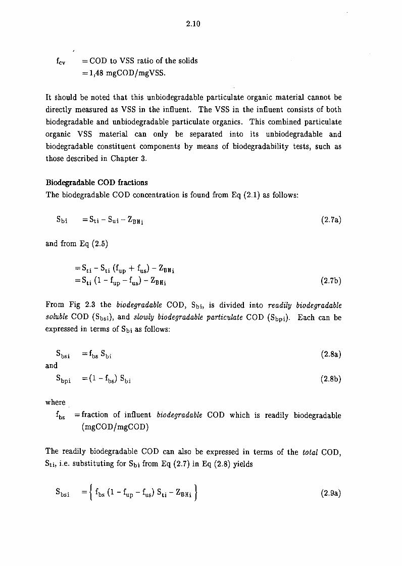
2.10
fcv = COD to VSS ratio of the solids
= 1,48 mgCOD/mgVSS.
It should be noted that this unbiodegradable particulate organic material cannot be
directly measured as VSS in the influent. The VSS in the influent consists of both
biodegradable and unbiodegradable particulate organics. This combined particulate
organic VSS material can only be separated into its unbiodegradable and
biodegradable constituent components by means of biodegradability tests, such as
those described in Chapter 3.
Biodegradable COD fractions
The biodegradable COD concentration is found from Eq (2.1) as follows:
= Sti - Sui··· ZBHi
and from Eq (2.5)
= Sti - Sti (fup + fus) - ZBHi
= Sti (1 - fup - fus) - ZBHi
(2. 7a)
(2.7b)
From Fig 2.3 the biodegradable COD, Shi, is divided into readily biodegradable
soluble COD (Sbsi), and slowly biodegradable particulate COD (Sbpi). Each can be
expressed in terms of Sbi as follows:
sbsi = f bs sbi and
sbpi = (1 - fbs) sbi
where
(2.8a)
(2.8b)
fbs = fraction of influent biodegradable COD which is readily biodegradable
(mgCOD/mgCOD)
The readily biodegradable COD can also be expressed in terms of the total COD,
Sti, i.e. substituting for Sbi from Eq (2. 7) in Eq (2.8) yields
(2.9a)

2.11
(2.9b)
where
fts = fraction of influent total COD which is readily biodegradable
(mgCOD/mgCOD).
For BEPR systems, the readily biodegradable COD (Sbsi) is subdivided in
fermentable readily biodegradable COD (Sbsfi) and SCFA (Sbsai), i.e.
(2.10)
Each of these can be expressed in terms of Sbsi as follows:
(2.11)
(2.12a)
(2.12b)
where
f = fraction of readily Sbs>a biodegradable COD which is SCFA
(mgCOD/mgCOD)
fsbs>f = fraction of readily biodegradable COD which is fermentable
(mgCOD/mgCOD)
The SCFA can be expressed also in terms of the total COD, Sti, i.e.
(2.13)
where
fs,bsa = fraction of total COD which is readily biodegradable SCF A
(mgCOD /mgCOD)
2.3.3 Typical wastewater COD characteristics
Values for typical South African wastewater COD characteristics are listed in
Table 2.1. Table 2.1 shows that for raw (unsettled) wastewater, about 7% of the
total COD is unbiodegradable soluble, 15% unbiodegradable particulate, 58% slowly

2.12
biodegradable (particulate) and 20% readily biodegradable (soluble).
2.4 FACTORS INFLUENCING WASTEWATER CHARACTERISTICS
A number of factors influence the characteristics or nature of the wastewater to be
treated. Broadly these can be divided into the following categories:
• Input to the sewer
• Transformations in the sewer
• Physical/chemical treatment prior to the activated sludge system.
2.4.1 Input to the sewer
Input to the sewer depends on the community served. The relative contribution by
industry and the types of industry discharging to the sewer have a major effect on
wastewater characteristics ( e.g. on maximum specific growth rate of nitrifiers ). The
wastewater characteristics presented above are valid for municipal wastewaters with
a relatively minor industrial contribution, < say 30% of COD load (WRC, 1984).
For the domestic portion of the wastewater, a number of factors are of importance:
Availability of water resources ( restricted water resources cause low water usage
with resultant high strength > 1 500 mgCOD/t, low flow wastes and vice versa), socio-economic status of the community (higher income communities use more
water per capita), community diet ( consumption of meat, etc), use of detergents
(phosphorus based or phosphorus free), customs (use of garbage grinders, etc), use of
on-site pretreatment ( e.g. septic tanks), are some of the many factors of major
importance. For example, caution should be exercised when selecting an
unbiodegradable particulate COD fraction (fup): Social organization of the
community for whom the wastewater treatment system is envisaged can have a
substantial influence on this parameter. Analyses of data reported by Sutton et al.
(1979) from Canada indicate that the fup fraction is 0,25 for raw wastewater. Such
a high value probably arises from the use of garbage grinders. A similarly high fup
is used in the design procedure followed by Black and Veatch (1979) [based on
McKinney's activated sludge model] which includes an unbiodegradable organic
material fraction which is equivalent to an fup value of 0,23. Wastewaters with high
fup fractions will result in greater sludge production than those with low fractions
and selecting too low a value will result in under provision of reactor volume and
sludge handling facilities.
The use of separate or combined sewers has a major influence on wastewater

2.13
characteristics, in particular on wastewater strengths and flows: Combined sewers
have greatly reduced strengths due to dilutions, and much larger flows with
increased variability due to storm flows than separate sewers. In South Africa
separate sewers are mandatory by legislation; in Europe a mixture of combined and
separate sewers are used. The degree of infiltration into the sewer by rainwater or
sand/grit etc. will also influence the wastewater characteristics and therefore
wastewater treatment plant behaviour.
2.4.2 Transformations in the sewer
In its transport through the sewer, the wastewater may undergo transformations.
The nature and extent of these transformations will depend on the conditions
prevailing in the sewer; residence time, temperature, aeration state and scour
velocity. For anaerobic sewers with long residence times, sulphate reduction and
acid fermentation may occur; for aerobic sewers, COD reduction and significant
growth of heterotroph (and sometimes even autotroph) active biomass may occur.
In South Africa, sewers are predominantly anaerobic so that heterotroph active
biomass growth is restricted and residence times short so that very little acid
fermentation occurs.
2.4.3 Physical/chemical treatment prior to the activated sludge system
For the activated sludge system in the wastewater treatment plant, the preceding
unit operations for physical treatment will influence the wastewater characteristics.
While unit operations such as grit removal, fats and oils removal by, for example,
dissolved air flotation, will exert some influence, the unit operations that have a
dominant effect are primary sedimentation and flow balancing. With primary
sedimentation, the COD load on the activated sludge system is considerably reduced
( ± 40% ), but a smaller reduction is obtained for the TKN and total phosphate, TP
( ± 15-20%). This has the effect that settled wastewaters have higher TKN /COD
and TP /COD ratios than raw wastewaters, see Table 2.1.
In Europe chemically assisted primary sedimentation to effect chemical P removal is
sometimes implemented. This significantly increases the COD removal (to around
60%) and produces a settled wastewater with very low COD, high free and saline
ammonia (FSA), and low orthophosphate (OP). Primary sedimentation with or
without chemical assistance, has a marked effect on the relative contribution of the
COD fractions because the particulate [ eg. components ( eg. Sup, Sbp)] are removed,
the soluble components (eg. Sus, Sbs) not. This causes that the soluble COD, TKN

2.14
and TP fractions make up a larger proportion of the remaining settled wastewater
COD, TKN and TP concentrations than in raw wastewater. The reduced COD
loads through including primary sedimentation have a marked effect on the design;
sludge production, reactor volume, oxygen demand, etc. will all be reduced, (WRC,
1984).
With the implementation of biological excess phosphorus removal, acid fermentation
of primary sludge is a desirable option. This has the effect of decreasing the
TP /RBCOD ratio, making the conditions for P removal more favourable (see
Wentzel et al., 1990; Pitman, 1991).
With flow balancing, the daily COD, TKN and TP loads to the plant are not
affected with the result that the biological reactor volume is not reduced. However,
flow balancing reduces the amplitudes in diurnal flow load variations which cause a
marked reduction on peak oxygen demand, and secondary settling tank surface area
(WRC, 1984).
2.5 CLOSURE
In this Chapter characterization of the wastewater carbonaceous (C) material
fractions (measured in terms of the COD parameter), required for design and
simulation models, has been described. There are numerous pitfalls in selecting
wastewater characteristics uncritically and without recognition of the factors which
contribute to the nature and composition of the wastewater - the importance of
careful and considered wastewater characteristic selection must be emphasized as
the system design and predicted response will only be as good as the selected
wastewater characteristics are representative of the particular wastewater. For this
reason it is imperative that for design and simulation of activated sludge systems,
the wastewater fractions are accurately quantified. To achieve this, experimental
measurement techniques must be available that are simple and practical to use, yet
still provide estimates with acceptable accuracy. In the next Chapter the
experimental techniques available in the literature to quantify wastewater
C fractions will be reviewed.

Ga
s
To
tal
Infl
ue
nt
Bio
rea
cto
r W
as
te s
tre
am
(P
art
icu
late
)
Bio
de
gra
da
ble
14
x
1 .i
Un
bio
de
gra
da
ble
Bio
log
ica
l T
ran
sfo
rma
tio
ns
I _
__
__
__
-. _
__
__
__
_ I
Eff
lue
nt
So
lub
le
Fig
2.1
:
2° s
ett
ling
ta
nk
Pa
rtic
ula
te U
nd
erf
low
R
ecycle
Pa
rtic
ula
te
Div
isio
n of
in
flue
nt
was
tew
ater
ca
rbon
(C
),
nitr
ogen
(N
) an
d ph
osph
orus
(P
) m
ater
ials
ac
cord
ing
to
the
biol
ogic
al
and
phys
ical
pr
oces
ses
in t
he a
ctiv
ated
slu
dge
syst
em.
Eff
lue
nt
So
lub
le
I
t..:>
-Cll

Total Influent
2.16
Biodegradable Unbiodegradable
Fig 2.2:
Particulate Soluble
The general wastewater characterization structure for carbon (C), nitrogen (N) and phosphorus (P) material.
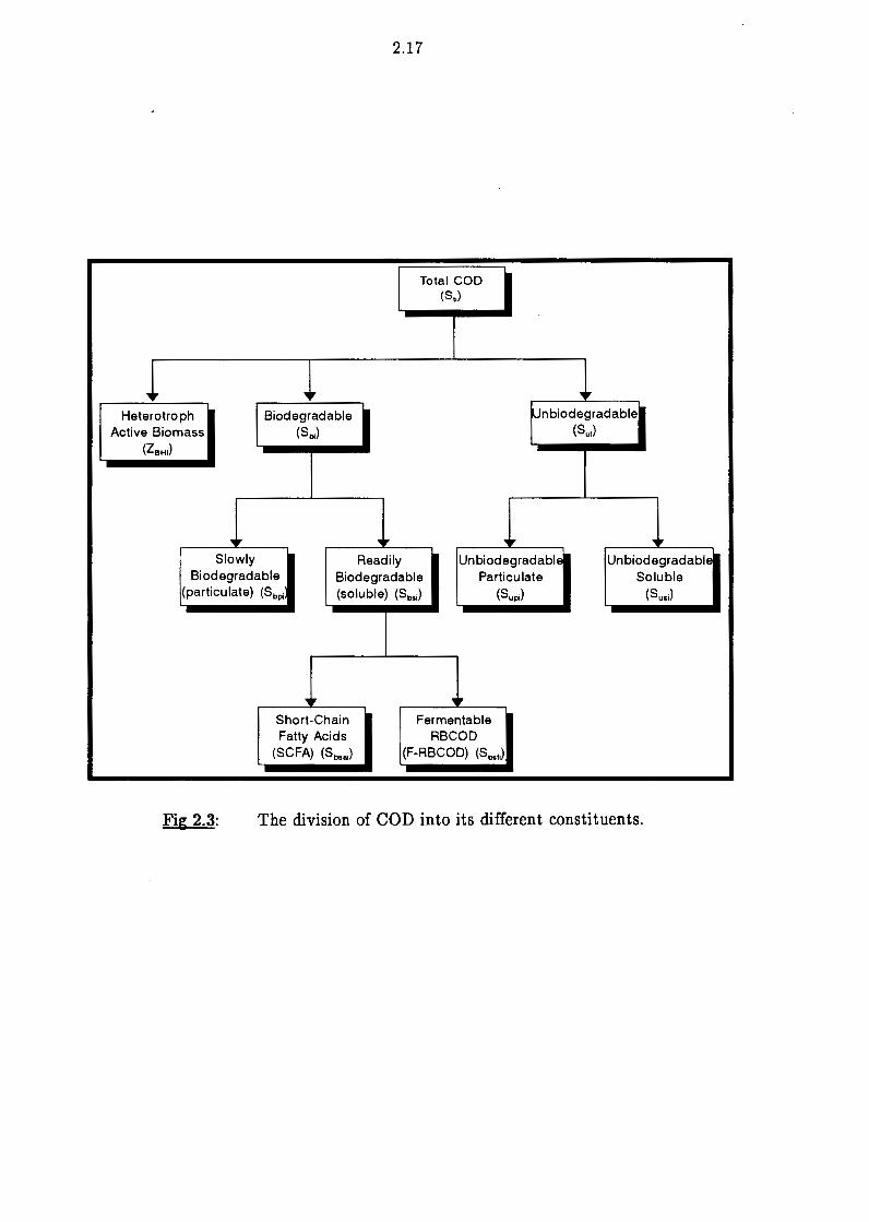
2.17
Total COD (Sti)
"II Ill" , .. Heterotro ph Biodegradable Unbiodegradable
Active Biomass (Sbi) (Suil
(ZeH;)
,,. """ "II,. ,,.
Slowly Readily Un biodegradable Un biodegradable Biodegradable Biodegradable Particulate Soluble
(particulate) (Sbpi (soluble) (Sbsi) (Supi) (Susi)
"Ir """ Short-Chain Fermentable Fatty Acids RBCOD
(SCFA) (Sbsa;) (F-RBCOD) (Sbs1;)
Fig 2.3: The division of COD into its different constituents.

TAB
LE 2
.1:
Rep
rese
ntat
ion
of
the
ma
gn
itud
e o
f th
e d
iffe
ren
t C
OD
fra
ctio
ns
in a
typ
ica
l S
ou
th A
fric
an
mu
nic
ipa
l w
ast
ew
ate
r.
WA
ST
EW
AT
ER
CO
MP
ON
EN
T
TY
PIC
AL
RA
NG
E O
F V
ALU
ES
U
NIT
S
SY
MB
OL
DE
SC
RIP
TIO
N
RA
W
SE
TT
LED
CO
D
sti
To
tal
infl
ue
nt
CO
D c
on
cen
tra
tio
n
50
0 -
1 2
00
3
50
-7
50
m
gC
OD
/£
fus
Fra
ctio
n o
f to
tal
CO
D w
hic
h i
s u
nb
iod
eg
rad
ab
le s
olu
ble
0
,04
-0,
10
0
,05
-0
,20
m
gC
OD
/mg
CO
D
fUD
Fra
ctio
n o
f to
tal
CO
D w
hic
h i
s u
nb
iod
eg
rad
ab
le p
art
icu
late
0
,07
-0
,20
0
,00
-0
, 10
m
gC
OD
/mg
CO
D
fts
Fra
ctio
n o
f to
tal
CO
D w
hic
h i
s re
ad
ily b
iod
eg
rad
ab
le (
solu
ble)
0
,08
-0
,25
0,
10
-0
,35
m
gC
OD
/mg
CO
D
fbs
Fra
ctio
n o
f b
iod
eg
rad
ab
le C
OD
wh
ich
is
read
ily (
solu
ble)
0
, 10
-0
,30
0,
12
-0
,40
m
gC
OD
/mg
CO
D
fsbs
a
Fra
ctio
n o
f re
ad
ily b
iod
eg
rad
ab
le (
solu
ble)
CO
D w
hic
h i
s S
CF
A
0, 1
0 -
0,4
0
0, 1
0 -
0,4
0
mg
CO
D/m
gC
OD
fsbs
f
Fra
ctio
n o
f re
ad
ily b
iod
eg
. (s
olub
le)
CO
D w
hic
h i
s fe
rme
nta
ble
0
,60
-0
,90
0
,60
-0
,90
m
gC
OD
/mg
CO
D
fcv
CO
D/V
SS
ra
tio
1,4
5 -
1,5
0
1,4
5 -
1,5
0
mg
CO
D/m
gV
SS
FsR
s
Fra
ctio
n o
f to
tal
CO
D r
em
ove
d i
n p
rim
ary
se
ttlin
g
0,3
0 -
0,6
0
-%
OT
HE
RS
µn
m
Ma
xim
um
sp
eci
fic g
row
th r
ate
of
nit
rifi
ers
0
,20
-0
,80
0
,20
-0
,80
/d
TK
N/C
OD
In
flu
en
t T
KN
/CO
D r
atio
0
,07
-0,
10
0
,09
-0
, 12
m
gN
/mg
CO
D
TP
/CO
D
Infl
ue
nt
TP
/CO
D r
atio
0
,01
5 -
0,0
25
0
,02
-0
,30
m
gP
/mg
CO
D
BO
D5
Infl
ue
nt
BO
D5
con
cen
tra
tio
n
25
0 -
60
0
15
0 -
37
5
mg
BO
D/£
Tmin
M
inim
um
te
mp
era
ture
1
0 -
15
10
-1
5
oc
Tmax
M
axi
mu
m t
em
pe
ratu
re
20
-3
0
20
-3
0
oc
Alk
A
lka
linit
y 2
00
-4
00
2
00
-4
00
m
g/£
as
Ca
C0
3
t-:> ......
00

CHAPTER 3
EXISTING METHODS FOR QUANTIFICATION OF WASTEWATER COD FRACTIONS
3.1 INTRODUCTION
In Chapter 2 the basis for subdivision of the influent wastewater carbonaceous
materials (measured in terms of the COD parameter) into a number of fractions has
been set out. In this Chapter existing methods to quantify these COD fractions will
be reviewed, to identify their strengths and weaknesses and to select the more
promising for evaluation and further development.
3.2 QUANTIFICATION METHODS
3.2.1 Readily biodegradable COD (RBCOD) measurement
The readily biodegradable COD (RBCOD) has been identified as being of
fundamental importance in design and operation of N (van Haandel et al., 1982) and
N and P (Siebritz et al., 1983; Wentzel et al., 1985; Nicholls et al., 1985; Wentzel
et al., 1990; Pitman, 1991) removal systems; the magnitude of both N and P
removal has been linked to the magnitude of the influent RBCOD.
A number of methods have been proposed for measure~ent of RBCOD. These can
be categorized as (1) physical or (2) bioassay methods.
(1) Physical methods:
The division of the biodegradable COD into the two fractions, RBCOD and slowly
biodegradable COD (SBCOD) was originally based on the observed difference in
response of activated sludge system biomass to the two fractions (see Chapter 2),
i.e. the division was biokinetically based (Dold et al., 1980; see Chapter 2). It has
been hypothesized that the difference in biokinetic response of activated sludge to
RBCOD and SBCOD (see Chapter 2) is due to differences in molecule size -
RBCOD consists of relatively small molecules that are readily transported into the
cell whereas SBCOD consists of larger more complex molecules that require
breakdown (hydrolysis) to smaller units before uptake and utilization (Dold et al.,
1980; Dold et al., 198fl; see Chapter 2). Accordingly, physical separation of the two
biodegradable COD fractions on the basis of molecular size has been proposed as an
approximation of the biokinetic division. For the physical separation, filtration has
been proposed. The basis for the filtration method is that influent wastewater
3.2
' samples are filtered and the COD of the filtrate determined. Ideally, both the
biodegradable and unbiodegradable soluble fractions (i.e. RBCOD and Susi
respectively) would be present in the filtrate. To separate out the unbiodegradable
soluble COD fraction (Susi), effluent from an activated sludge reactor is also filtered
and the COD of the filtrate determined. Noting that all the biodegradable soluble
COD (i.e. RBCOD) will be removed in the activated sludge system, provided the
sludge age is in excess of about 3 days, then the effluent filtrate COD should
provide a close estimate of the unbiodegradable soluble COD (Suse)- Assuming that
the unbiodegradable soluble COD in the effluent (Suse) equals the influent
unbiodegradable soluble COD (Susi), then the biodegradable soluble COD (i.e.
RBCOD) can be found by difference, i.e.
RBCOD = (influent - effluent) filtrate COD.
Two problems are apparent in assessing this proposed method (Dold et al., 1986):
(1) It is assumed that the effluent filtrate COD closely equals the influent
unbiodegradable soluble COD (Susi)- This implies that there is no significant
generation of unbiodegradable soluble COD within the system.
(2) The soluble/colloidal material in municipal wastewaters may span a wide
range of molecular sizes and weights. The problem is to select an appropriate
filter pore size that will give a separation that matches the biokinetic division
of the biodegradable COD, that is, a filter pore size, which will allow the
passage of RBCOD (and unbiodegradable soluble COD) through, but will
retain the SBCOD (and unbiodegradable particulate COD).
These two aspects are dealt with below.
A. Effluent Filtrate COD:
The filterable (or "soluble") portion of the effluent COD from an activated sludge
system is made up of a wide range of organic compounds. Dold et al. (1986) have
reviewed a number of investigations that used a variety of experimental techniques
to characterize and fractionate secondary effluents. Amongst these methods were,
sedimentation and centrifugation ( e.g. Hunter and Heukelekian, 1960), dialysis
membranes (e.g. Bunch et al., 1961), ultrafiltration membranes (e.g. Saunders and
Dick, 1981), gel permeation chromatography (e.g. De Walle and Chian, 1974). In

3.3
comparing the results from these investigations, Dold et al. (1986) conclude that
secondary effluents contain a wide range of organics, from low molecular weight
volatile acids to high molecular weight polymeric compounds.
With regard to the origin of these compounds, there are three possible sources: (1)
the influent COD, (2) intermediates and end products of metabolic pathways, and
(3) products from cell lysis and death. In terms of the proposed filtration methods,
all organics in the filtered effluent are assumed to originate from (1) the influent
COD. It is assumed that the contribution from the other two possible sources is
negligible. Information in the literature on this aspect is reviewed below:
(2) Intermediates and end products: Products of the metabolic activities of
organisms in a system will be present within the organisms, and may
accumulate to appreciable levels ( as a result of, for example, malfunctions in
the control mechanisms). Because the accumulated products will diffuse out
of the cell at a rate proportional to the concentration gradient across the cell
membrane, these materials, although possibly degradable, will be present in
the liquid phase and therefore also in the effluent - the magnitude of the
residual amount of this material will depend inter alia on the rate of its
degradation (Chudoba et al., 1969; Grady and Williams, 1975; Daigger and
Grady, 1977).
Perhaps the strongest evidence demonstrating the presence of intermediates
and end products in the effluent is the molecular weight fractionation work of
Leidner et al. (1984) using low-pressure gel chromatography: In Fig 3.1, the
lower line shows the molecular weight distribution (MWD) of the dissolved
organic carbon (DOC) in the effluent from a laboratory unit treating a
mixture of glucose and glutamic acid; the upper line represents the MWD of
the influent. Component-selective tests for glucose and glutamic acid in the
effluent were negative, indicating that the DOC in the effluent was derived
from microbial sources only. Parallel tests were conducted on cell-free
extracts of the biomass from the system, see Fig 3.2. That is, samples of
sludge were centrifuged, washed and broken up to release the liquid contents
(extract); the particulate matter then was removed by filtration. As is
apparent in Fig 3.2, MWD fractionation of the cell-free extract showed only
two peaks for compounds at the extremes of the range. These peaks appear
to correspond to the two peaks at the extremes in the effluent MWD plot

3.4
(Fig 3.1). This strongly supports the proposal that products of the metabolic
activities of organisms in a system are present in the effiuent. These results
were corroborated by Grady et al. (1984), who also identified two peaks in the
effiuent MWD using ultrafiltration fractionation and COD measurements.
(3) Cell lysis products: Researchers have also proposed that residual matter from
cell lysis and death will add to the soluble COD from microbial origin
(Saunders and Dick, 1981; Gloor et al., 1981; Leidner et al., 1984; Chudoba,
1985; Namkung and Rittman, 1986). Again confirmatory evidence for this
proposal is provided by the results of Leidner et al. (1984). The MWD in Fig
3.2 for the cell-free extract exhibits only two peaks, whereas the effiuent
MWD in Fig 3.1 exhibits an indistinct distribution of compounds between the
two peaks. This intermediate weight fraction would suggest that compounds
present in the effluent have their origin from a source other than the influent
or organism intermediate and end products, namely cell lysis products. The
widespread MWD of these compounds would suggest that lysis products
produced are subject to some degree of hydrolysis and degradation.
From the review above, it is evident that there exists a strong possibility for
generation of unbiodegradable soluble COD in the activated sludge system, either
from organism intermediate and end products or cell lysis products. However, the
review provides no guidance on the relative magnitude of this generation compared
to the unbiodegradable soluble COD derived from the influent. The magnitude of
the contribution of the two microbial sources above to the effluent soluble COD will
determine the viability of the proposed separation method. If the contribution is
large then the method will fail because the assumption that the unbiodegradable
soluble COD in the effluent is near equal to that in the influent will be incorrect.
However, if the microbial generation within the system is small compared to the
influent soluble COD fractions (RBCOD, Sbs, and unbiodegradable soluble COD,
Sus), then the error introduced in the test will be small.
Some guidance on this aspect can be found in the literature. The experimental work
of Chudoba (1985) on batch and continuous flow laboratory systems treating
artificial pure biodegradable substrates has shown that the effluent COD is
approximately 1 percent of the influent COD, that is, for an influent COD of 500
mgCOD/l the effluent COD, which must originate from microbial activity, would
be 5 mgCOD/l. With the pure substrate glucose as influent feed, Germirli

3.5
et al. (1991) and Boero et al. (1991) found that microbial generation was higher than
that observed by Chudoba et al., approximately 2,5 to 3 percent of influent COD.
This would indicate that for an influent COD of 500 mgCOD/.t, approximately
15 mgCOD/.t would be microbially generated. Assuming that similar quantities of
unbiodegradable soluble COD are generated in a wastewater treatment plant, then
for a municipal wastewater of 500 mgCOD/.t the amount generated of
5-15 mgCOD/.t may be significant compared to typical measured filtered effluent
CODs of 25-60 mgCOD/.t (WRC, 1984). Comparing the highest measured
microbial unbiodegradable soluble COD generated (15 mgCOD/.t) with the expected
RBCOD (50-150 mgCOD/.t), the error introduced by neglecting microbial
generation may be significant. However, in the literature quoted above artificial
substrates were used. In the municipal wastewater treatment plant, due to the
diversity of organics making up the influent it is likely that a much more diverse
population would develop than in the artificial substrate fed systems. This should
result in an increase in utilization of the microbially generated organics m
wastewater treatment systems compared to pure cultures, or cultures grown on
limited artificial substrates.
The work of Dold et al. (1986), Mamais et al. (1993) and Torrijos et al. (1994) using
municipal wastewaters appears to confirm the above conclusion. Dold et al. (1986)
and Mamais et al. (1993) compared results obtained using the proposed filtration
method (i.e. assuming negligible microbial unbiodegradable soluble COD formation)
with the conventional bioassay tests and found close correlation (see later). Torrijos
et al. (1994) in an extensive investigation on quantifying wastewater COD fractions,
monitored the degradation of different soluble COD molecular sizes in batch tests.
They concluded that the distribution of organic compounds after degradation was
closely equal to that before degradation, that is, no significant unbiodegradable
soluble COD generation took place.
From the review above it would appear that generation of unbiodegradable soluble
COD by microbial action in the activated sludge system does take place, but is
negligible compared to that derived from the influent. However, any methods
proposed that are based on the separation concept will have to be extensively
evaluated by comparing the results with conventional bioassay tests.
B. Selection of filter pore size:
The soluble/colloidal material in municipal wastewaters may span a wide range of

3.6
molecular sizes and weights. The problem is to select a filter pore size that will give
a separation that matches the biokinetic division of the biodegradable COD, that is,
a filter pore size that will allow the passage of RBCOD (and unbiodegradable
soluble COD, Sus) through but will retain the SBCOD (and unbiodegradable
particulate COD, Sup). Filtration methods with various filter pore sizes have been
used ( e.g. Dold et al., 1986; Lesouef et al., 1992; Mamais et al., 1993; Bartone et al.,
1994; Torrijos et al., 1994). In evaluating the effect of pore size, Dold et al. (1986)
found that for domestic wastewater, membranes with cut-off < 10 000 molecular
mass gave RBCOD that closely correlated with those determined by the
conventional bioassay methods, see Fig 3.3. In contrast Bartone et al. (1994) found
that with an industrial (textile) wastewater, membranes with cut-off < 10 000
molecular mass gave RBCOD very much lower (13% of total COD) than that
measured in bioassay batch tests (20% of total COD). Recognizing that facilities
for this type of ultrafiltration were not widely available, Dold et al. (1986) evaluated
0,45µm filters and found that with domestic wastewater a fraction of SBCOD
and/or Sup passed through the filter causing the RBCOD to be overestimated, see
Fig 3.4. Using 7-8 µm glass fibre filter papers the data of Lesouef et al. (1992)
indicated similar results. To overcome this problem, Mamais et al. (1993)
successfully investigated flocculation of colloidal material (SBCOD and/or Sup)
before filtration through 0,45µm filters and obtained estimates for RBCOD that
compared very favourably with those from the conventional flow-through
square-wave bioassay test (see later). Torrijos et al. (1994) in an extensive
investigation of the characteristics of a domestic wastewater, found that O,lµm
filters gave a true indication of RBCOD without the need for preflocculation.
In all the filtration methods, since both biodegradable and unbiodegradable soluble
COD pass through the filter, the unbiodegradable fraction has to be quantified
independently and subtracted from the COD of the filtrate to give the RBCOD.
This requires effluent from a continuous flow-through activated sludge system (Dold
et al., 1986; Bartone et al., 1994) or sequencing batch reactor (Mamais et al., 1993;
Torrijos et al., 1993) which may not be available, or measurements of filtered COD
over at least 10 days in batch tests (Lesouef et al., 1992), a time-consuming task.
Of the filtration methods proposed, that of Mamais et al. (1993) appears to hold the
most promise. By including the preflocculation step, the uncertainty regarding filter
pore size appears to have been largely eliminated. Also, ultrafiltration, which is not
widely available, does not have to be used - 0,45µm filters appear to be adequate for

3.7
this method. Accordingly the Mamais et al. method will be investigated in this
research project.
(2) Bioassay methods:
Since the division between RBCOD and SBCOD is based on a biological response
rather than a physical phenomenon, tests in which the response of activated sludge
to wastewater is monitored, bioassay tests, have found wider application than the
physical methods. A variety of bioassay tests have been developed to measure
RBCOD. The basis for these tests is that environmental conditions are created
which allow the difference in response of organisms to RBCOD and SBCOD to be
monitored and separated.
Separation of the response of the biomass to RBCOD and SBCOD is based on the
different rates of utilization of RBCOD and SBCOD (see Chapter 2). The rate of
RBCOD utilization is much higher than that of SBCOD utilization, by an order of
magnitude (Dold et al., 1980). Because the rate of RBCOD utilization is higher,
and its proportion in the wastewater much less than that of SBCOD, conditions can
be created whereby the RBCOD and SBCOD are utilized simultaneously, and then
SBCOD only is utilized. The difference between these two responses gives the
response due to RBCOD utilization only. The bioassay tests to measure RBCOD
can be categorized into three groups:
( 1) Continuous flow-through activated sludge systems.
(2) Aerobic batch test methods.
(3) Anoxic batch test methods.
Each of these methods is described below.
A. Continuou.s flow-through activated sludge systems
This method involves monitoring the oxygen utilization rate ( OUR) response in a
single reactor aerobic activated sludge system with sludge recycle, operated at a
sludge age of about 2 to 3 days under daily cyclic square wave loading conditions
(12 hours with feed, 12 hours without feed). On feed termination there is a
precipitous decrease in OUR after which the OUR remains near constant for a
period before decrea8ing to a rate associated with endogenous respiration, see
Fig 3.5. This behaviour was hypothesized to be due to the following (Dold et al.,
1980; Ekama et al., 1986): During the feed period both RBCOD and SBCOD are

3.8
added to the reactor via the influent, and used simultaneously. The rate of
utilization of RBCOD is system limited, that is, the RBCOD is utilized as fast as it
is fed and so the feed rate limits the rate of utilization and the RBCOD
concentration remains virtually zero. In contrast, the SBCOD is process limited,
that is, the SBCOD is fed faster than the biomass can utilize it so that the biomass
SBCOD maximum specific utilization (growth) rate limits the rate of utilization and
SBCOD will accumulate in the reactor. On feed termination the supply of both
RBCOD and SBCOD via the influent ceases. Since the RBCOD has been virtually
completely consumed during the feed period, utilization of RBCOD also ceases and
accordingly the OUR exhibits a precipitous drop. Since SBCOD has accumulated in
the reactor during the feed period, utilization of SBCOD must continue. The
conditions in the reactor (short sludge age, high load period) causes the utilization
of SBCOD to continue at the maximum rate giving rise to the OUR plateau
observed after feed termination. Also, the conditions in the system cause that
nitrification, if present, continues at a maximum rate after feed termination. Thus,
the precipitous drop in OUR observed after feed termination is due entirely to the
RBCOD and hence the drop in OUR allows the RBCOD concentration to be
determined (for details see Ekama et al., 1986).
Sollfrank and Gujer et al. (1991) in an investigation of this method found difficulty
in maintaining a constant temperature in the reactor on feed termination. They
concluded that these variations in temperature will influence the nitrification rate,
and so lead to an error in the RBCOD concentration determined from the
precipitous drop in OUR. Accordingly, they proposed that nitrification be inhibited
by addition of allyl thiourea ( A TU) and that the loading rate be decreased by
increasing the sludge age (to approximately 5 days). They found that these
modifications improved the temperature stability in the system. However, the
proposed increase in sludge age will increase the mass of organisms in the reactor
which will cause SBCOD to be utilized more rapidly and so lead to situations where
SBCOD does not accumulate sufficiently during the feed period to enable the
SBCOD utilization to continue after feed termination for a period adequate to
clearly identify the OUR plateau.
Although the continuous flow-through method has become the standard for
measuring RBCOD, the method has been criticized for its cost and difficulty of
operation (Sollfrank and Gujer, 1991 ).

3.9
,
B. Aerobic batch test method.
In this method a volume of wastewater is mixed with a volume of mixed liquor in
an aerated and stirred batch reactor, and the OUR response monitored with time
(e.g. Ekama et al., 1986; Henze, 1991; 1992).
With the correct selection of the volumes of wastewater and mixed liquor, on mixing
in the aerated, stirred batch reactor, the OUR remains constant at a plateau for a
period of up to 3 hours depending on the wastewater RBCOD concentration,
whereafter the OUR drops precipitously, then levels off at a second plateau, see
Fig 3.6. This OUR-time profile is made up of the OURs for nitrification and for
carbonaceous material utilization.
If ammonia concentration is greater than about 2 times the half saturation constant
for nitrification (in the Monod formulation for the growth rate of the nitrifying
autotrophs), the nitrification will take place at a maximum (and constant) rate.
Consequently, if adequate ammonia is available at the start of the batch test ( which
is normally the case with domestic wastewater), and since the half saturation
constant for the autotrophs is relatively small (KsA = 1,0 mgN/t, Dold et al., 1980;
Henze et al., 1987), the nitrification rate will remain at a maximum and constant
value over the test period giving rise to a constant nitrification OUR (Fig 3.6,
Area 3).
Superimposed on the constant nitrification OUR is the OUR due to carbonaceous
material utilization [Fig 3.6, Area 1 + Area 2(a & b)] which gives rise to the
variation in the observed OUR with time. The interpretation of the carbonaceous
OUR-time profile is as follows:
RBCOD and SBCOD are utilized independently but simultaneously by the
heterotrophs for growth; RBCOD is directly absorbed and utilized while SBCOD is
adsorbed extracellularly, hydrolyzed to smaller units which then are utilized
directly. The summation of the OURs associated with RBCOD and SBCOD growth
gives rise to the observed carbonaceous OUR. At the start of the batch test both
RBCOD and SBCOD are present, and are utilized independently for growth, with
associated OURs (Fig 3.6, Area 1 for RBCOD, Area 2a for SBCOD). The OUR is
constant over the initial period because the RBCOD and SBCOD concentrations are
sufficiently high to ensure that RBCOD utilization and SBCOD
hydrolysis/utilization rates are close to their respective maxima. Once the influent

3.10
RBCOD is depleted, the OUR drops to the second plateau which is due to the
maximum hydrolysis/utilization of SBC OD only (Fig 3.6, Area 2b ). The magnitude
of the drop in OUR is proportional to the heterotroph maximum specific growth
rate on RBCOD, µH, and can be used to obtain an estimate for this constant (Fig
3.6). Also, the area under the OUR-time profile associated with RBCOD (Fig 3.6,
Area 2) can be used to calculate the wastewater RBCOD concentration (see Ekama
et al., 1986; Dold et al., 1991).
In operation of this test, the mass of COD (i.e. V ww *Sti, where Sti = total COD
concentration of the undiluted wastewater and Vww = volume of wastewater) with
respect to the mass of VSS (i.e. V mi*Xv, where Xv = VSS concentration and V ml = volume of mixed liquor) mixed in the batch test is known as the COD loading rate
(LR). The LR established in the batch test should be such that the OUR response
is well defined and allows (1) the initial peak OUR to be readily determined, (2) the
magnitude of the precipitous drop in OUR to be clear, and (3) the area under the
initial peak OUR (Fig 3.6, Area 1) to be accurately estimated (to calculate
RBCOD). For the same wastewater volume changing the LR does not change the
magnitude of Area 1, which is a function only of the mass of RBCOD in the
wastewater sample, but it does change the shape of Area 1: If LR is too low (i.e. a
higher mixed liquor volume), the shape is tall and narrow because the RBCOD is
utilized very quickly, and too few measurements can be taken to give reasonable
surety of initial high OUR; if LR is too high, the shape is low and wide and it is
difficult to establish the magnitude of the drop in OUR (see Fig 3.7).
Selection of the optimal loading rate is not a simple task. The rate at which the
organisms utilize the RBCOD (i.e. maximum specific growth rate), and hence the
duration of the initial plateau, depends upon inter alia the conditions under which
the mixed liquor has been generated (Ekama et al., 1986). If the mixed liquor has
been subjected to high LR (e.g. selector reactor) then it will exhibit rapid RBCOD
utilization due to a high maximum specific growth rate.
The aerobic batch test method has been used successfully to derive estimates for
RB COD ( e.g. Ekama et al., 1986; Henze 1992; Kappelar and Gujer, 1992).
However, for this method sludge acclimatized to the wastewater has to be obtained,
either generated in special laboratory-scale continuous flow-through reactor (Ekama
et al., 1986; Sollfrank and Gujer, 1991; Kappelar and Gujer, 1992) or from a
full-scale plant (Nicholls et al., 1985). The requirement of a laboratory-scale

3.11
,
reactor for sludge generation for the batch method test does not resolve criticisms
levelled at the flow-through method, while the option of obtaining a sludge from a
full-scale plant may not be available if a new plant is to be designed and built.
Furthermore, in batch tests the use of sludges from biological excess P removal
(BEPR) systems will produce erroneous results for RBCOD due to the phenomenon
of RBCOD uptake and storage with P release by polyP organisms under aerobic and
anoxic conditions without the utilization of oxygen or nitrate (Still et al., 1986;
Wentzel et al., 1989a; 1989b ).
C. Anoxic batch test method.
The basis of this test is identical to that for the aerobic batch test described above.
The only difference is that instead of aerating the batch test contents and measuring
the OUR, nitrate is added at the start of the test and the nitrate concentration is
monitored over a period of approximately 4 to 5 hours (see Fig 3.8). In the absence
of dissolved oxygen, nitrate serves the same function as oxygen, i.e. as electron
acceptor. Therefore, in the anoxic batch test the nitrate concentration initially will
decrease at a constant rapid rate reflecting the rate of utilization of RBCOD as well
as SBCOD from the wastewater. The initial rapid rate of denitrification is
constant, because the concentration of RBCOD is so high that the growth rate of
the heterotrophs is at its maximum (µH) in accordance with Monod kinetics. Once
the RBCOD from the influent is depleted, the denitrification rate reduces (i.e. the
decrease in nitrate takes a flatter linear slope, Fig 3. 7) to the rate of utilization of
SBCOD; this slower denitrification rate is analogous to the second plateau in the
aerobic batch test. The RBCOD concentration can be calculated from the mass of
nitrate utilized during the initial rapid denitrification rate, see Ekama et al. (1986)
and Henze (1991) for details.
With the anoxic batch test, the same restrictions and cautions identified for the
aerobic batch test also apply.
Summary
The bioassay tests by their nature provide a good estimate for RBCOD - the
concept of RBCOD (and SBCOD) was developed from observations made on one of
the bioassay tests, the continuous flow-through system (Dold et al., 1980; Ekama
et al., 1986). However, the bioassay tests all have a common shortcoming in that
they require mixed liquor acclimatized to the wastewater being tested: In a
continuous flow-through test this is generated in the same reactor in which the test

3.12
' is done; in the batch test procedures it must be generated either in separate
laboratory-scale reactors, or obtained from full-scale plants. The operation and
maintenance of laboratory-scale systems is a difficult and costly exercise. Obtaining
mixed liquor from a full-scale plant may not be possible if the plant is to be
designed and built. Furthermore, as noted earlier mixed liquor from a biological
excess phosphorus removal (BEPR) plant cannot be used in the batch test
procedures.
From the above, it is evident that a bioassay test that does not require
preacclimatized mixed liquor would be of considerable benefit; one of the intentions
of this research was to develop such a test.
3.2.2 RBCOD subfractions
In Chapter 2 it was noted that if biological excess phosphorus removal (BEPR) is to
be included in the activated sludge system, the RBCOD must be subdivided into
two subfractions, short-chain fatty acids (Sbsai) and fermentable RBCOD (Sbsfi).
A simple titration procedure has been presented in the literature to quantify Sbsai
(Moosbrugger et al., 1992;1993). With Sbsai and RBCOD quantified, Sbsfi can be
determined by difference. Since a method is available in the literature,
quantification of the RBCOD subfractions will not be addressed in this research
project.
3.2.3 Influent heterotrophic active biomass measurement
The original UCT model (Dold et al., 1980; van Haandel et al., 1981) did not
consider active biomass or autotroph biomass to be present in the influent; for
municipal wastewaters in South Africa, the sewers generally are short (retention <6
hours) and anaerobic, and were considered unlikely to support active biomass
generation. Further, simulations with the UCT model appeared to support this
supposition. However, investigations in Europe have indicated that European
municipal wastewaters can contain a significant heterotroph active biomass fraction
(Henze, 1989), up to 20% of the total COD (Kappelar and Gujer, 1992). Seeding of
this influent biomass to the activated sludge system can have a significant influence
on modelling and design. For example, seeding of heterotroph active biomass with
the influent can significantly influence the response of the activated sludge system at
low temperatures, by ensuring that "washout" of organisms does not occur.
Similarly, seeding of autotrophic biomass will cause that nitrification will be
maintained at shorter sludge ages and/or lower temperatures than expected. These

3.13
findings have highlighted the need for a simple test to quantify this wastewater
fraction.
In the literature there is scarcity of information on tests to quantify this wastewater
fraction. Microbiological techniques have been proposed for analysis of mixed liquor
from activated sludge systems which possibly could find application in wastewater
characterization. For example, colony counts using a pour plate method ( Gaudy
and Gaudy, 1980), DNA analysis (Liebeskind and Dohmann, 1994; Blackall, 1994)
and others. However, the majority of these techniques are still in their infancy,
have not yet been adequately integrated with design and kinetic modelling theory
and, in any event, require very sophisticated equipment and techniques that are not
widely available. It is unlikely that these tests will find routine application in the
design of activated sludge systems.
In contrast, Kappelar and Gujer (1992) describe a simple batch test to quantify
heterotrophic active biomass in the activated sludge; a small quantity of activated
sludge is mixed with centrifuged wastewater and oxygen utilization rate ( OUR)
response monitored with time. From the observed exponential increase in the OUR,
the initial OUR in the batch test can be quantified which can be used to derive an
estimate for the heterotroph active biomass concentration (see Chapter 4).
Kappelar and Gujer note that the test can be adapted to quantify the heterotroph
active biomass in wastewater by excluding the activated sludge, but details of this
modification are sparse. However, the proposals of Kappelar and Gujer appear to
hold promise for further development and will be investigated in this research.
3.2.4 Unbiodegradable soluble COD measurement
Measurement of the influent unbiodegradable soluble COD (Susi) is relatively
simple: For sludge ages greater than 3 days, all the RBCOD is consumed in the
biological reactor and the SBCOD and particulate unbiodegradable COD are
enmeshed in the mixed liquor and will settle out in the secondary settling tank (see
Chapter 2). Thus, the only soluble COD from the influent that will be present in
the effluent is the Sus· Furthermore, it can be assumed that the generation of
unbiodegradable soluble COD by microbial action in the activated sludge system is
negligible compared to that derived from the influent (for a detailed discussion on
this aspect see Section 3.2.1 above). Accordingly, the effluent soluble COD in a
long sludge age activated sludge system will equal Susr By running a steady state
laboratory-scale unit at a sludge age greater than 3 days and measuring the filtered
3.14
(0,45µ.m) effluent COD, Suse can be determined; at steady state Susi = Suse
(Ekama et al., 1986). The difficulty with this method to determine Susi is that
running laboratory-scale activated sludge systems can be a time consuming and
costly task. Lesouef et al. (1992) have shown that Susi can be determined from an
aerated batch test as the filtered COD after 10 days. With the method of Lesouef
et al., there is considerable delay in obtaining an estimate for Susi (10 days). This
research will investigate whether it may be possible to reduce the length of time
required for the batch test without detrimentally affecting the estimate for Susi·
3.2.5 Unbiodegradable particulate and slowly biodegradable CODs measurement
Measurement of influent unbiodegradable particulate (Supi) and slowly
biodegradable (Sbpi) COD fractions present difficulties as both contribute to the
mixed liquor solids in the biological reactor (see Chapter 2): Measurement of the
mixed liquor solids does not distinguish between the components making it up -
active biomass, endogenous mass, Supi and Sbpi, see Fig 3.9. Supi and Sbpi can be
estimated simultaneously by running a laboratory-scale unit at a long sludge age,
say 15 days or longer, and comparing the measured mixed liquor volatile suspended
solids (VSS) concentrations and carbonaceous oxygen consumptions to those
calculated using theoretical design equations (WRC, 1984) with different Supi values
(Ekama et al., 1986). The values for Supi that give theoretical VSS and
carbonaceous oxygen consumption equal to those measured will be the same
provided the COD mass balance is 100%. If the COD mass balance is not 100%,
using the VSS comparison will provide the more accurate estimate for Supi· A long
sludge age is selected because the mixed liquor VSS concentration becomes more
sensitive to Supi as the sludge age increases. Having found Supi, Susi and Sbsi, Sbpi
then can be found by difference. Overall, the Supi, Susi and Sbpi must provide
consistency between theoretical and measured responses at different sludge ages
(Ekama et al., 1986). It is evident that determining Supi and Sbpi by running
laboratory-scale activated sludge systems is a time consuming and costly exercise.
Furthermore, Supi (and thus Sbpi) can be estimated only via the hypothesized
design equations (WRC, 1984) and in this regard it has meaning only in terms of
the model structure.
Sollfrank and Gujer (1991) have proposed a method to determine Sbpi that provides
an estimate in a relatively short time. The wastewater is centrifuged and the pellet
is spiked into an activated sludge system in which the feed has been stopped. By
monitoring the OUR response, an estimate of Sbpi could be obtained. However, not

3.15
,
all the Sbpi present in the wastewater will be centrifuged into the pellet; some will
remain suspended in the supernatant so that the method will underestimate Sbpi·
The Sbpi in the supernatant will have to be determined independently. Sollfrank
and Gujer (1991) proposed that this be done in separate batch tests in which the
supernatant is added to mixed liquor and the OUR response monitored. Due to the
low concentration of particulate material in these batch tests compared to the high
concentrations of soluble biodegradable material, it is unlikely that accurate
estimates for Sbpi can be derived.
Kappelar and Gujer (1992) proposed that Sbpi be determined from the aerobic batch
test described above for RBCOD determination, see Fig 3.6. After the precipitous
drop in OUR, the OUR is due to nitrification and particulate carbonaceous material
utilization. Kappelar and Gujer (1992) eliminated nitrification from the batch test
by adding the inhibitor ATU. Thus, the OUR following the precipitous drop is due
to SBCOD utilization only. However, this SBCOD is that derived from the influent
and that formed from the death/lysis of heterotroph active biomass added to the
batch test with the mixed liquor. Separation in a batch test of the OUR due to
each of these two sources of SBCOD is not easy and introduces fairly large errors in
the estimate of Sbpi, a problem that will become evident in the research presented
here (see Chapter 8).
3.3 CONCLUSION
Quantification of the influent wastewater COD fractions is of crucial importance for
modelling and design of wastewater treatment systems. Existing procedures to
quantify wastewater COD fractions are either too elaborate or approximate; the
need exists for simple, reliable methods for accurate estimation of these parameters.
From the review above, it would appear that two tests in particular hold promise
for further evaluation and development:
• The flocculation/filtration method of Mamais et al. (1993).
• The batch test method of Kappelar and Gujer (1992).
In this research project these two methods will be investigated.

Fig 3.1:
Fig 3.2:
u 0 0
3.16
60
>5000 -3000 <200
Molecular weight distribution of dissolved organic carbon (DOC) in the influent and effluent of laboratory activated sludge system treating a mixture of glucose and glutamic acid. (After Leidner et al., 1984).
u 0 C
60 120
2
>5000 -3000 <200 Molecular Weight
180 3 h
Molecular weight distribution of dissolved organic carbon (DOC) in the cell-free extract of sludge in a laboratory activated sludge system treating a mixture of glucose and glutamic acid. (After Leidner et al., 1984).

Fig 3.3:
Fig 3.4:
200 190 180 170
'"'
"' 160 0 150 0 u 140 0,
E 130 ...., L 120 0 ~ 110 ;: 0 100 L ..
90 5 0 80 0 70 ~
~ 60 >-I 50 ti .0 40 in
30 20 10 /
/ 0
0
/ /
/ /
/ /
/ /
/ /
/
3.17
+ + //
+ / + /
• 0 O / T }/ ++
+ / 0
~i/ /
/ /
0 0
/
/ /
/ /
/ /
/
/ /
/
/ /
/ /
/
20 40 60 80 100 120 140 160 180 - 200
Sbsi-Squore wove method (mgCOD/1)
Examples of daily data pairs for a number of sewage batches, values of readily biodegradable COD (Sbs) determined by ultra-filtration plotted versus values obtained by the flow-through square wave method. (After Dold et al., 1986).
200 190 180
·'°' 170
..::. :60 Cl 0 150 (.)
140 OI
E 130 'J
L 120 0 .. 110 ..
C 100 0
90 L u
E 80
Ill 70 ,t
60 0 I 50
"ii 40 .0
in 30 20 10 /
/
0
0
/ /
/ /
/ /
/ /
/ /
+ + + + ++ •+ + + + /
+ ++ / \ ++-1 + +//
+ ""+.++l +++/ + t... + / t ++-.:r+ )/
t * ++ / + ~· / )-/ + + .... +-+t + /T'
/f / +
/ /
/ /
/ /
/ /
/
/ /
/ /
/
20 40 60 80 100 120 140 160 180 200
Sbsi-Squore wove method (mgC00/1)
COD of raw wastewater 0,45µm filtrate plotted versus corresponding values of the readily biodegradable COD (Sbs) obtained by the flow-through square wave method. (After Dold et al., 1986).

3.18
OUR (mg0/1/h} 50
Start feed
40
•• I •
30 I • • I
20 I ~. 10
•••••
Stop
1 feed ...... ..., • •••• • ...
• • • ••• ••
0 L-..L...---'----'---"---'-.......J....---1....--1-----'.-----l.--'-!....-..__..,____.__--'----'--'-----l....--'---'-----.1.--'-'--'
0
Fig 3.5:
5 10 15 20 25
Time (h)
OUR response over one cycle in an aerobic activated sludge unit subjected to daily cyclic square wave feed (12h feed on, 12h feed off) with municipal wastewater as influent. (After Ekama et al., 1986).

20
Fig 3.6:
OUR (mg0/1/h)
2
3.19
µH IAWPRC
3
Time (h)
4 5
OUR-time profile for aerobic batch test with activated sludge addition, with nitrification. (After Dold et al., 1991).
OUR (mg0/1/h) 140.----------------------~
120
100
80
LR too low LR=Loading Rate
Correct LR
LR too high
0 .___ ____________________ __._ ___ ____... ___ __..
0
Fig 3.7:
1 2 3 4 5
Time (h)
OUR-time profile for aerobic batch test to show the effect of loading rate on the shape of the OUR-time plot. (After Dold et al., 1991).

""'
' z I ,,,
0 z OI
E .._, z 0 j:: < D:: I-z L&J (J z 0 (J
L&J I-< D:: !: z
Fig 3.8:
40
35
30
25
20
15
10
5
3.20
··~··············-r·····r······· ....
q_~ j ,6.1 N03
.......... ~~ ...... ~ .... J... ~N03
- - Cl .
........ ~:-:.--:~~.Cl ........... . - -ci a ._a
-0'?3 g_ Cl..._
a "2. lil...o._ At ----, a CN:l.o ..Q.
0 -a a -g_ !J-.c c Q...
0 +---.--,---,---,--,---,---,--,---,---.--,---r----.--.---r----.--.....---1
0 20 40 60 80 100 120 140 160 180
TIME (mlnutH)
Example of nitrate concentration-time plot in an anoxic batch test for measuring the influent readily biodegradable COD concentration. (After Ekama et al., 1986).

Fig
3.9
:
Tot
al
Su
spe
nd
ed
S
olid
s (T
SS
)
Ino
rga
nic
Su
spe
nd
ed
+
Vo
latil
e S
usp
en
de
d
Sol
ids
(IS
S)
So
lids
(VS
S)
Xv
~
Bio
rea
cto
r jx
BH +
xE
j+[3
] Xv
= X
8H
+ X
E+ X
,
I 'I
XsH
+ X
E I
I B
iolo
gic
al
I I T
ran
sfo
rma
tion
~
1__?
2_!
~e-±
2H
2S
----
-,
I
_J_
__
__
_
r 1.
I
20 S
ettli
ng
Eff
lue
nt i
.ilsu
se =
Sus
i I
Tan
k ,
.
Un
de
rflo
w
Re
cycle
XsH
+XE
+x,
Sch
emat
ic r
epre
sent
atio
n of
the
tra
nsfo
rmat
ions
of
the
infl
uent
C
OD
fr
acti
ons
wit
hin
the
acti
vate
d sl
udge
sys
tem
.
c:,..,
tv
1-4

CHAPTER4
BATCH TEST FOR MEASUREMENT OF READILY BIODEGRADABLE COD AND ACTIVE ORGANISM CONCENTRATIONS
IN MUNICIPAL W ASTEWATERS
4.1 INTRODUCTION
Quantification of influent wastewater RBCOD and heterotroph active biomass is of
crucial importance for modelling and design of wastewater treatment systems.
Further, from the review in Chapter 3 the need exists for simple, reliable methods
for accurate estimation of these parameters. To this end, in this Chapter the batch
test proposal of Kappelar and Gujer (1992) in which the OUR response of
wastewater is monitored with time, will be refined and developed, to measure
simultaneously the influent heterotroph active biomass and RBCOD concentrations.
4.2 TEST PROCEDURE
The batch test was done on wastewater samples without activated sludge seed. The
wastewater samples were unsettled because the active organisms, being particulate,
would largely settle out in the primary settling tank. The procedure for the batch
test was as follows: A defined volume (3.t) of unsettled municipal wastewater,
obtained from either Mitchell's Plain or Borcherds Quarry Treatment Plants, Cape
Town was placed in a continually stirred batch reactor maintained at a constant
temperature of 20° C. A sample was drawn to obtain the initial total COD
concentration (Standard Methods, 1985). In operating the batch test, the surface of
the wastewater was covered by small plastic balls to limit surface exchange of
oxygen. The OUR was monitored continually using an automated technique
(Randall et al., 1991) ·- the DO was raised to 6 mgO/t, the air switched off and the
decrease in DO monitored, the rate of decrease giving the OUR; when the DO
reached 4 mgO / t, the air was switched on again and the cycle repeated. The pH of
the reactor was monitored continually and controlled to pH 7 ,5 ( :1:: 0 ,2). Because of
the low OUR values, regularly during an aeration cycle the walls of the reactor were
thoroughly brushed to prevent particulate matter sticking to them. At intervals
samples were drawn from the reactor, filtered (0,45µm) and analyzed for nitrate and
nitrite. The tests were run for approximately 20 hours. At the end of the test the
contents of the batch reactor were homogenized in a liquidizer, a sample drawn and
total COD concentration measured.

4.2
,
4.3 RESULTS
Using the results of one batch test on Mitchell's Plain wastewater as an example,
the OUR (mgO/t/h) versus time (h) response is shown plotted in Fig 4.1. The
initial and final COD concentrations were 821 and 481 mgCOD/t respectively. No
nitrate or nitrite was detected in the test indicating the absence of nitrification, that
is, no autotrophic biomass was present in the wastewater. Should the presence of
nitrifiers in the wastewater be a possibility, allyl thiourea probably can be used as a
nitrification inhibitor ( due to the absence of nitrification, addition of allyl thiourea
was not tested).
Referring to the OUR-time plot (Fig 4.1 ), during the first period of the batch test
( < 7 t h) the OUR exhibits an exponential increase due to heterotroph active
biomass growth. After ::1: 7 t h, the OUR drops precipitously due to depletion of the
RBCOD. For the remainder of the batch test, the OUR exhibits an inverted S
pattern typical of saturation kinetics, due to SBCOD utilization.
4.4 DATA INTERPRETATION
The data from the batch test can be interpreted in terms of either the UCT (Dold
et al., 1980; 1991) or IA WQ (Henze et al., 1987) models. For this investigation, the
UCT model was selected, using the data from Fig 4.1 as a worked example;
interpretation in terms of IA WQ model does not present undue difficulty and is also
briefly presented.
For application of the UCT model to the batch test, the model can be greatly
simplified by recognizing that specific conditions prevail:
• Aerobic conditions - denitrification processes need not be included.
• No nitrification - nitrification processes need not be included.
• Excess ammonia present - nitrate as a N-source for growth need not be considered.
- transformations from organic to ammonia nitrogen need not be included.
Accepting these conditions, the UCT model can be simplified to that presented in
Table 4.1. In terms of this model the following information can be obtained from
the batch test:
• COD recovery (%).
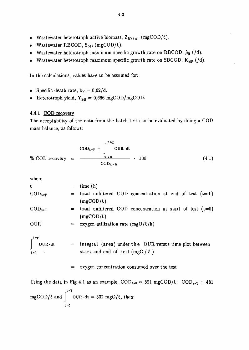
4.3
• Wastewater heterotroph active biomass, ZBH< oi (mgCOD/t).
• Wastewater RBCOD, Sbsi (mgCOD/t).
• Wastewater heterotroph maximum specific growth.rate on RBCOD, µ,H (/d).
• Wastewater heterotroph maximum specific growth rate on SBCOD, KMP (/d).
In the calculations, values have to be assumed for:
• Specific death rate, bH = 0,62/ d.
• Heterotroph yield, Y ZH = 0,666 mgCOD/mgCOD.
4.4.1 COD recovery
The acceptability of the data from the batch test can be evaluated by doing a COD
mass balance, as follows:
% COD recovery -
t =T
CODt=T + I OUR dt
t = 0 • 100 (4.1)
where
t
CODt=T
CODt=O
OUR
t=T I OUR·dt
t =O
CODt= o
time (h)
total unfiltered COD concentration at end of test (t=T)
(mgCOD/t)
- total unfiltered COD concentration at start of test ( t=O)
(mgCOD/.t)
- oxygen utilization rate (mgO/t/h)
integral (area) under the OUR versus time plot between
start and end of test (mgO / t )
- oxygen concentration consumed over the test
Using the data in Fig 4.1 as an example, CODt=O = 821 mgCOD/t; CODt=T = 481
t=T mgCOD/.t and J OUR·dt = 332 mgO/t, then:
t =O

4.4
481 + 332 01_ % COD recovery= 821
• 100 = 99,o.
Mass balances between 95-105% indicate that the test results are acceptable, and
these were generally obtained in most batch tests without undue difficulty ( see
Chapter 5).
4.4.2 Wastewater heterotroph active biomass, ZBH< ol
From the simplified UCT model (Table 4.1), the rate of growth of heterotroph
biomass (dZBH/dt) is given by:
dZBH -- = growth on RBCOD + growth on SBCOD - death dt
where
ZBH =heterotroph active biomass concentration (mgCOD/t)
Sbs =RBCOD concentration (mgCOD/t)
KsH = half saturation constant for RBCOD
=5 mgCOD/t
Sads =adsorbed SBCOD concentration (mgCOD/tJ
Ksp = half saturation constant for SBCOD
=0,027 mgCOD/mgCOD
(4.2)
It can be accepted that during the initial stages of the batch test (before RBCOD is
depleted and the OUR drops precipitously) Sbs » KsH and Sads/ZBH » Ksp, and
therefore,
(4.3)
Integrating Eq ( 4.3) and solving yields the active organism concentration at time t
[ZBH< ti, mgCOD/t] in terms of the initial active organism concentration [ZBH< ol,
mgCOD/t], time (t, in h) and the net specific growth rate (µH + KMp-bh) viz;
(µH + KMp-bH)t/24 ZBH< ti = ZBH< oi e (4.4)

4.5
' The OUR at time t (OURt, mgO/t/h) is a function of ZBH( ti and the net specific
growth rate
1-YzH OUR< tJ = (µH + Kyp) ZBH< tJ /24 (4.5)
YzH
Substituting Eq (4.4) for ZnH<tJ in Eq (4.5) and taking natural logs yields
(4.6)
which is a straight line with,
slope (4.7)
[ 1-YzH ]
y-intercept = tn ( OURc t=ol ) = tn (µH + Kyp) ZnH col /24 YzH
(4.8)
From a plot of tn OURc tJ versus time (h), ZnH< oi can be obtained:
(ey-intercept). 24
ZBH< Ol - (mgCOD/t) (4.9) 1-YzH -- • (slope•24 + bH)
YzH
The OUR values for the data in Fig 4.1 up to the precipitous drop in OUR, are
shown plotted tn OUR versus time (h) in Fig 4.2. Linear regression yields,
tn OUR= 1,2814 + 0,297 t (R2 = 0,998).
Accepting Y ZH = 0,666 mgCOD/mgCOD and bH = 0,62/d (the value for bH is
probably less for the raw sewage in the batch test than the 0,62/d for normal
activated sludge systems because predators probably will not be present in
significant concentrations; however, a reduced value for bH has relatively little
influence since µH + KMP » bH), and inserting into Eq ( 4.9) yields:

4.6
e 1,2814 • 24 ZBH< ol = ---------- = 22 mgCOD/L
1-0,666 (0,297·24 + 0,62)
0,666
This represents 22/821 · 100 = 2, 7% of the wastewater COD, a very minor fraction.
In terms of the IAWQ model, growth and OUR are due to utilization of RBCOD
only, either directly from RBCOD in the influent or from RBCOD generated by
SBCOD hydrolysis. However, this does not influence determination of ZBH( o>
except that (µH + KMP) in the equations above is equivalent to the maximum
specific growth rate, µH*, in the IAWQ model. Accordingly, Eq (4.9) above can be
used directly to determine ZBH( o> in terms of the IAWQ model.
4.4.3 Heterotroph maximum specific growth rate on SBCOD, KMP
The RBCOD concentration is calculated from the concentration of oxygen utilized
in its degradation. This requires the OUR before the precipitous drop to be
separated into its RBCOD and SBCOD contributions, which is equivalent to
separating the overall growth rate (i.1,H + KMP) into its JLH and KMP components.
These calculated values for µH and KMP from the batch test are unlikely to be of
value in modelling activated sludge system. The organism population that develops
in the activated sludge system is likely to differ appreciably from that which
develops in the batch reactor since the conditions present in the batch test (high
COD, low active biomass) differ significantly from those in the activated sludge
system (low COD, high active biomass). Consequently, the two populations
probably will have different kinetic constants.
In terms of the UCT model, growth of heterotrophs on RBCOD and SBCOD is
independent. The OUR's (mgO/t/h) associated with these two growth processes
are given by Eq ( 4.5) which can be separated to give:
(1) 1-Y ZH (µ + K b )t/24
OURRBCOD(t) ·24= • JLH • ZBH(Ol •e H MP- H (4.10) YzH
(2) (4.11) YzH
Up to the precipitous decrease, the OUR is the sum of both the RBCOD and

4.7
SB COD utilization [Eq ( 4.10) + Eq ( 4.11)]. Once the RB COD is depleted, which
causes the precipitous OUR decrease, the OUR is that for SBCOD only [Eq (4.11)].
If the precipitous decrease occurs at t=s hours .at which time the OUR is
OURsBCOD<t=sl, then from Eq (4.11) KMP is given by
where
OURsBCOD( t=s l · 24
1-YzH -- • ZBH< Ole YzH
(4.12)
OURsBCOD< t=sJ - OUR due to SBCOD only, i.e. observed OUR immediately
following the precipitous drop in OUR (mgO/l/h).
(t=s) - time immediately following the precipitous drop in OUR (h)
(µH + KMP-bH)/24 = slope of ln OURc ti versus time (h) plot.
Using the data in Figs 4.1 and 4.2 as an example, time s = 7,8h; OURsBCOD< t=7,Shl
= 11,2 mgO/l/h; slope of ln OURc ti vs time plot = 0,297 (Fig 4.2); ZBH< ol = 22
mgCOD/l:
11,2 • 24 KMP = ---------- = 2,4/d
1-0,666 ___ ,
22 • e0,297 • 7,8
0,666
In the IAWQ model, utilization of RBCOD and SBCOD is not independent; only
RBCOD is utilized, either from that present in the wastewater or from SBCOD
hydrolysis. However, to interpret the data in the batch test to calculate the
RBCOD present in the wastewater, distinction has to be made between the RBCOD
in the wastewater and the RBCOD generated from hydrolysis of SBCOD. To do
this, the approach developed here for the UCT model can be followed.
Conceptually, in the IA WQ model this amounts to independent utilization of the
two "types" of RBCOD, but does not influence the value calculated for influent
wastewater RBCOD. To determine the contribution of SBCOD hydrolysis to the
RBCOD, the maximum specific hydrolysis rate, KH, in the IAWQ model needs to
be calculated, as follows:

4.8
(mgCOD/mgCOD/d) ( 4.13)
For the example presented here,
KH= 2,4/0,666 = 3,6 mgCOD/mgCOD/d.
4.4.4 Heterotroph maximum specific growth rate on RBCOD, µ1
For the UCT model, the value for µH can be calculated from the value for KMP
derived above and the slope of the ln OUR versus time plot, as follows
( 4.14)
For the example,
µH = 0,297 • 24 - 2,4 + 0,62 = 5,4/d.
For interpretation in terms of the IA WQ model,
(4.15)
For the example,
µH* =5,4 + 2,4 = 7,8/d.
4.4.5 Determination of the influent RBCOD concentration
Knowing KMP and µH individually, the OURsBCOD can now be subtracted from
OURtotal to give the OURaBCOD· The RBCOD then is given by 1/(1-Y zH) times
the area between the observed OUR and the theoretical OURsBCOD from the start of
the batch test (t=O) to the precipitous drop (t=d):
l t=d
RBCOD = --I (OURtotal - OURsBCOD) dt 1-YzH
t =O
l t=d
= --J OURancoD dt 1-YzH
t =O
(mgCOD/l) (4.16)
( 4.17)

4.9
The RBCOD concentration can be found by doing the integration in Eq ( 4.16)
graphically or that in Eq ( 4.17) analytically. For the former, the OURsBCOD from
Eq ( 4.11) with KMP = 2,4/d is shown plotted in Fig 4.1. The area between the
observed OUR and the theoretical OURsBCOD was determined to be 68,9 mgO/t.
Therefore, RBCOD = [1/(1-0,666)] ·68,9 = 206 mgCOD/.t.
For the latter, Eq (4.17) is integrated analytically by substituting Eq (4.10) for
OURaBCOD and solving the definite integral between t=O and t=d, viz.:
RBCOD - µH • ZBH( Ol {eslope·td - 1}
YzH · slope-24 (mgCOD/.t) (4.18)
where
td = time of precipitous drop in OUR (h)
slope = slope of .tn OUR versus time (h) plot
For the example, µH = 5,4/d; ZBH<ol = 22 mgCOD/l; YzH - 0,666 mgCOD/
mgCOD; slope = 0,297; td = 7 ,4 h:
5,4·22 RBCOD = {e01297 · 7,4 -1} = 200 mgCOD/.t
0,666·0,297•24
In a comparative test, the results for the conventional flow-through test (Ekama
and Marais, 1979) for the same batch of wastewater gave RBCOD = 207
mgCOD/.t.
In terms of the IA WQ model, to determine the influent RBCOD an artificial
division of the observed OUR has to be made, between OURaBCOD for influent
RBCOD utilization and OURsBCOD for utilization of RBCOD generated from
SBCOD hydrolysis. Equations for these OURs can be derived from the IAWQ
model. These are identical to Eqs (4.10) and (4.11) except that
µH + KMP in UCT = µH* in IA WQ.
Jl,tt in UCT = µH*-Ktt/Y ZH in IAWQ.
KMP in UCT = Ktt/YzH in IAWQ.

4.10
Equation ( 4.18) for the RB COD concentration also applies except that µH is
replaced by µH*-KH/Y ZH as indicated above.
4.5 CLOSURE
A batch test method has been presented to determine two influent wastewater COD
fractions, heterotroph active biomass and readily biodegradable COD (RBCOD).
The method has advantages over previous methods in that:
• The experimental procedure is relatively simple.
• No mixed liquor acclimatized to the wastewater is required.
• Independent determination of unbiodegradable COD is not necessary.
• The only independent constants required for calculation are the heterotroph yield
(Y zH) and specific death rate (bH); the procedure is relatively insensitive to the
value for bH. All other constants required for calculations are obtained from the
experimental data. However, it is unlikely that these constants (UCT model, µH and KMp; IAWQ model, µH* and KH) will be of much value in modelling and
design of activated sludge systems - most probably a population will develop in
the activated sludge system that differs appreciably from that in the wastewater
since the conditions in the wastewater (high COD, low active mass) differ
significantly from those in the activated sludge system (low COD, high active
mass).
The batch test method presented in this Chapter provides a simple means to
quantify two of the five influent wastewater COD fractions, namely readily
biodegradable COD and heterotroph active biomass. The accuracy of these
estimates will be evaluated in Chapter 5. Attempts to extend the batch test to
quantify also the remaining three COD fractions, unbiodegradable soluble COD,
unbiodegradable particulate COD and slowly biodegradable particulate COD are set
out later in this report.

..........
.c. --:::::::. 0 0)
E -a: ::> 0
Fig 4.1:
..........
.c. --:::::::. 0 0)
E -a: ::> 0 C
Fig 4.2:
4.11
30
25
20
15
10
5 ~, OUR SBCOD I
0 0 2 4 6 8 10 12 14 16 18 20
3.5
3
2.5
2
1.5
1
Time (h)
OUR-time plot for aerobic batch test on raw municipal wastewater from Mitchell's Plain Treatment Plant.
• lnOUR = 1,2814+0,29t R"'2 = 0 998
' •
0 1 2 3 4 5 6 7 8 Time (h)
tn-OUR versus time for the measured OUR data in Fig 4.1 up to the precipitous drop in OUR.

Tab
le 4
.1:
Mat
rix
repr
esen
tati
on o
f th
e U
CT
mod
el (
Dol
d et
al.,
199
1),
sim
plif
ied
for
cond
itio
ns p
rese
nt i
n th
e ba
tch
test
.
CCJIP
OOND
I
1 2
3 4
5 6
7 8
2 BH
ZE
z,
sads
s_
sb
s Su
s 0
PROC
ESS
RATE
, pj
j
PROC
ESS
1 A
erob
ic g
row
th o
f z 8H
on
sbs
1 ·1
/YzH
-1-
YzH
~
[ sb
s ]
YzH
l'H ---
ZeH
IC5H
+Sbs
~ A
erob
ic g
row
th o
f z 8H
on
sads
1
·11Y
zH
-1-Y
zH
[ (S
ads/
ZeH
> ]
Ki4f>
ZeH
YzH
IC5p
+( S
ads/
Zbh
)
13 D
eath
of
ZBH
-1
fE
1 · f
E
"if Z
eH
~ A
dsor
ptio
n of
Sel
'ln
1 -1
IC
ASe
rwile
H<f
MA
-Sad
s/ZeH
>
Sto
ichi
omet
ric
cons
tant
s K
inet
ic c
onst
ants
Yz
H =
Het
erot
roph
yie
ld
II
ifH
z H
eter
otro
ph m
ax.
spec
ific
gro
wth
..
II
II
II
fE
= En
doge
nous
re
sidu
e Il
l ..
.. ..
rate
on
S Il
l II
II
..
ICSH
= H
ete
rotr
~ 1
/2 s
atu
rati
on
on
Sir'
fMA
= M
ax.
rati
o s
ad9tz
8H
I ..
.. ~
.. ..
u ~
~ Il
l II
ic;
;jp •
H
eter
otro
ph m
ax.
spec
ific
gro
wt
.. ra
te o
n ~
s
· i
Ill
Ill
-II
II
..
ICSP
= H
eter
otr
1/2
sat.
on
S ds
II
II
:§
.. ..
1l
1l
~ bH
=
Het
erot
roph
sp
ecif
ic d
eatR
ra
te
.. 0
"i i
0 ICA
=
Senm
sp
ecif
ic a
dsor
ptio
n ra
te
.. Il
l II
Il
l ..
L ..
~
II
II
f f
:g .c
: II
-:ii
II
:a
:a "i
0 >
"'
·-.. Il
l >,
. >,
. ..
II
u "'
! !
{,..,
1l
II
I
~
i ,..,
,.., ,..,
,.., ui
,..,
ui
,.., ,..,
. .;
.
g .
(/) .
. .
1i .
. ..
J ..
J ..
J (/
) ..
J ..
J ..
J ..
J L
..J
u I
:§ "Z
f -
--
--
->,
. -
-8
8' 8
8 8
8 .c
: 8
-8
8 ii
1:11
.. L
Ill
i u
0 u
0 u
L u
0 u
~ u
u ~
u ~
. ~
"E ~
~ ~
Ill
~
~
~
~
~
"O
II
.. ID
:E
w
:E
-
:E
C
:E
w
:E
"' :E
:::
, :E
0
:E
.:::.
,_.
,:...,

CHAPTER 5
EVALUATION OF BATCH TEST FOR MEASUREMENT OF READILY BIODEGRADABLE COD AND ACTIVE ORGANISM CONCENTRATIONS
5.1 INTRODUCTION
In Chapter 4 a batch test method was developed to quantify two wastewater COD
fractions, readily biodegradable COD (RBCOD) and heterotroph active biomass
concentrations. Results from one batch test were used as an example to illustrate
the method for calculation of the results. In this Chapter the intention is to
evaluate the results from a number of such batch tests. This is to be done by
comparing the RBCOD results derived from the batch test with those from the
conventional flow-through square wave method (Ekama et al., 1986; see Chapter 3).
For heterotroph active biomass concentration, no conventional test is available.
5.2 METHOD
Wastewater from two sources was used for the batch tests, Borcherds Quarry and
Mitchell's Plain Treatment Plants (Cape Town, South Africa). For both Treatment
Plants, sewer retention times are short (3 to 4 hours) and the conditions are
anaerobic; therefore it is expected that heterotroph active biomass concentrations in
both wastewaters should be low. Batches of raw (unsettled) wastewater were
obtained from the inlet works to the treatment plants and stored in stainless steel
tanks at 4 • C for a period of approximately two weeks. (Experience has indicated
that storage for a period longer than about three weeks leads to significant changes
in the sewage characteristics; storage for two weeks was selected to eliminate this
possibility). Regularly, the contents of the stainless steel tanks were thoroughly
mixed and wastewater samples drawn off into a plastic container. The wastewater
was brought to a temperature of 20° C by placing the container in a warm water
bath (:50° C) and stirring gently. For some batch tests the wastewater was diluted
to approximately 500 mgCOD/.t by addition of tap water so that the measured
OURs would not be excessively high. Using the wastewater, the batch test
procedure detailed in Chapter 4 was followed. A number of batch tests were
conducted on each batch of wastewater collected, see Table 5.1. From the batch
tests the following information was derived using the equations set out in Chapter 4:
• COD recovery (%). • Wastewater autotrophic active biomass.

5.2
• Wastewater heterotrophic active biomass.
• Wastewater heterotrophic maximum specific growth rate on RBCOD.
• Wastewater heterotrophic maximum specific growtl;t rate on SBCOD.
• Wastewater RBCOD.
For the RBCOD measurements, the values were evaluated by comparing the results
from the batch test with results from the conventional flow-through square wave
bioassay test, see Chapter 3 (WRC, 1984; Ekama et al., 1986). This unit was
operated as specified by Ekama et al. (1986) and received the same wastewater used
in the batch tests, at a concentration of 500:50 mgCOD/l.. For wastewater
heterotroph active biomass, no conventional tests are available.
5.3 RESULTS
Comprehensive data for all the batch tests are listed in Tables B.la to B.5b in
Appendix B. Plots of OUR-time profiles for each batch test are also given in
Appendix A. Typical OUR-time profiles for Borcherds Quarry and Mitchell's Plain
wastewaters are shown plotted in Figs 5.la and 5.2a respectively. The OUR-time
profiles for both wastewaters conform to that shown plotted in Fig 4.1 (Chapter 4).
5.3.1 COD recovery
For every batch test, total unfiltered COD concentrations at the start and end of
the test, and area under the OUR-time curves are listed in Tables B.la and B.lb in
Appendix B for wastewaters from Borcherds Quarry and Mitchell's Plain
respectively. For every batch test, % COD recoveries were calculated using Eq
(4.1) in Chapter 4 and are also listed in Tables B.la and B.lb in Appendix B. The
% COD recovery is a function of the batch test method and so should not be specific
to each batch of wastewater tested. Accordingly, statistical plots of % COD
recoveries for all the batch tests on wastewaters from Borcherds Quarry and
Mitchell's Plain were constructed. From the statistical plots the means and
standard deviations for the batch tests on the two wastewaters were determined.
Batch tests with % COD recoveries more than, or less than two standard deviations
from the mean were rejected for further analysis, that is, batch tests that did not
fall within the 95% confidence interval were rejected (3 batch tests for Borcherds
Quarry wastewater and 7 for Mitchell's Plain wastewater, see Appendix B, Tables
B.la and B.lb respectively). Statistical plots of the % COD recovery for the
accepted batch tests for Borcherds Quarry and Mitchell's Plain wastewaters are
given in Figs 5.3 and 5.4 respectively. (The method used to construct the statistical

5.3
, ,
plots and how to interpret them is given in Appendix C). From these plots, mean
COD recoveries for Borcherds Quarry and Mitchell's Plain were 96% and 99%
respectively, with standard deviations of the mean of .0,76% and 0,82% respectively.
It is evident that COD recoveries were good lending credibility to the reliability of
the measurements and the batch test itself.
5.3.2 Wastewater autotrophic biomass concentration
Nitrate concentration at the start and end of the batch tests was measured; the
results are listed in Appendix B, Tables B.2a and B.2b for Borcherds Quarry and
Mitchell's Plain wastewaters respectively. For wastewaters from both sources, no
significant increase in nitrate concentration could be detected, indicating that
autotrophic biomass was not present in significant concentrations in these
wastewaters. Accordingly, for further analysis of all batch tests on raw wastewater,
the effect of nitrification was ignored. Should nitrification be detected in the batch
test, allyl thiourea probably can· be used as a nitrification inhibitor. Due to the
absence of nitrification, the effect of adding allyl thiourea could not be tested.
5.3.3 Heterotrophic active biomass
Influent wastewater concentrations
Following the procedure set out in Chapter 4, for each batch test the OUR from the
start of the test until the precipitous drop in OUR was plotted as tn OUR versus
time; typical profiles are shown in Figs 5.lb and 5.2b for Borcherds Quarry and
Mitchell's Plain wastewaters respectively. Linear regression was used to analyze the
data to derive the y-intercept, slope and correlation coefficient (R2). Values for
these parameters for all the different batch tests on the various wastewater batches
are listed in Appendix B, Tables B.3a and B.3b for Borcherds Quarry and Mitchell's
Plain wastewaters respectively. From the y-intercept and slope, the heterotroph
active biomass could be calculated using Eq ( 4.9) in Chapter 4. Values for
heterotroph active biomass as percentage of the total starting COD concentration
for every batch test are also listed in Appendix B, Tables B.3a and B.3b. Statistical
plots of heterotroph active biomass (% of wastewater total COD concentration)
were constructed for each wastewater batch; for example see Figs 5.5 and 5.6 for
Borcherds Quarry and Mitchell's Plain wastewaters respectively. Batch tests with
heterotroph active biomass more than, or less than two standard deviations from the
mean were rejected for analysis, that is, batch tests that did not fall within the 95%
confidence interval were rejected ( these are shown marked in Tables B.3a and b ).
Statistical plots excluding the rejected data were constructed for each wastewater
5.4
batch. From these statistical plots the mean and standard deviation of the mean
were determined for each batch of wastewater; these values are listed in Table 5.2
for both Borcherds Quarry and Mitchell's Plain w_astewaters (see Table 5.1 for
wastewater source).
For Borcherds Quarry wastewater a statistical plot of the means of heterotroph
active biomass (%) for the different wastewater batches is shown in Fig 5.7. From
Fig 5. 7, the mean heterotroph active biomass as a % of wastewater total COD was
10,3% with standard deviation of the mean of 1,0%. The relatively high heterotroph
active biomass was unexpected; the retention time of the sewers at Borcherds
Quarry is short ( :1:: 3 hours) so that low influent heterotroph active biomass was
expected. From an investigation of the operational procedures at the Borcherds
Quarry Wastewater Treatment Plant it was found that regularly waste activated
sludge was recycled to the head of the works, and mixed with the incoming influent
wastewater upstream of the point from where wastewater was drawn for the batch
test. The recycled waste activated sludge was correctly detected in the batch test,
indicated by the high heterotroph active biomass values.
For Mitchell's Plain wastewater, from Table 5.2 the first two batches of wastewater
(batches 10 and 11) had low heterotroph active biomass with means of 4,0% and
3,0% of the total COD respectively; variability also was low with standard
deviations of the means of 0,6% and 0,2% respectively, the low heterotroph active
biomass was expected as the retention times for the Mitchell's Plain sewers also are
short (:1:: 4 hours). However, for the subsequent two wastewater batches (batches 12
and 13) and a further batch (batch 21 ), heterotroph active biomass concentrations
were considerably higher see Table 5.1; for example batch 13 mean is 10% with
standard deviation of the mean of 1,4%. From an investigation of the plant
operation at Mitchell's Plain Wastewater Treatment Plant it was discovered that
when wastewater batches 12, 13 and 21 were collected, waste sludge from the
activated sludge system was being recycled to the head of the works, because of
repairs to the sludge treatment facilities. Again, the recycled waste activated sludge
was correctly detected in the batch test. For the remaining wastewater batches,
recycling of waste activated sludge was not practised which is reflected in the lower
measured heterotroph active biomass. For the wastewater batches in which no
activated sludge was recycled, a statistical plot of the measured mean heterotroph
active biomass for the different wastewater batches is given in Fig 5.8; from the
plot the mean heterotroph active biomass is 6,1 % and the standard deviation of the

5.5
mean is 0,65%.
Results obtained from the batch test for heterotropb active biomass could not be
evaluated against results from any conventional test since no conventional tests are
available. However, the batch test consistently reflected changes in heterotroph
active biomass concentration that could be traced to plant operation.
5.3.4 Heterotroph maximum specific growth rates on RBCOD and SBCOD
These constants are required to determine the RBCOD concentration, see Chapter
4. For every batch test the maximum specific growth rate of the heterotrophs on
SBCOD (KMP) was determined using Eq (4.12) in Chapter 4 and the values are
listed in Appendix B, Tables B.4a and B.4b for Borcherds Quarry and Mitchell's
Plain wastewaters respectively. Statistical plots of KMP for each wastewater batch
were constructed; for example see Figs 5.9 and 5.10 for Borcherds Quarry and
Mitchell's Plain respectively. Batch tests with KMP more than, or less than two
standard deviations from the mean were rejected for analysis, that is, batch tests
that did not fall within the 95% confidence interval were rejected (these are shown
marked in Tables B.4a and b ). From the statistical plots the means and standard
deviations of the means for each wastewater batch, were determined, see Table 5.3
(see Table 5.1 for wastewater source). Statistical plots of KMP means for the
different wastewaters are shown in Figs 5.11 and 5.12 for Borcherds Quarry and
Mitchell's Plain respectively. Mean KMP values were 1,91/d and 2,47 /d for
Borcherds Quarry and Mitchell's Plain respectively, with standard deviation of the
mean of 0,10 and 0,20 respectively.
The maximum specific growth rates of the heterotrophs on RBCOD (µH) were
calculated using Eq (4.14) in Chapter 4 and are listed in Table B.4a and B.4b for
Borcherds Quarry and Mitchell's Plain wastewaters respectively. The JLH data were
evaluated in exactly the same fashion as described above for Kyp data. Examples of
statistical plots for µH for one wastewater batch from Borcherds Quarry and
Mitchell's Plain are shown in Figs 5.13 and 5.14 respectively; mean JLH and standard
deviation of the means are listed in Table 5.3 for the different wastewater batches
(see Table 5.1 for wastewater sources). Statistical plots of the JLH means for the
different wastewater batches are shown in Figs 5.15 and 5.16 respectively. Mean
values were 3,85/d and 4,38/d for Borcherds Quarry and Mitchell's Plain
respectively, with standard deviations of the mean of 0,30 and 0,12 respectively.
5.6
Comparing the values for KMP and µH obtained from the batch test with those
available in literature for activated sludge, KMP = 1,35 {/d) and µH = 1,5-3,5 {/d)
(Dold et al., 1991), the values obtained in the batch. tests are considerably higher.
Most probably a population develops in the activated sludge system that differs
appreciably from that in the wastewater ( measured in the batch tests), since
conditions in the wastewater (high COD, low active mass) differ significantly from
those in the activated sludge system (low COD, high active mass). Accordingly, it
is unlikely that the values for the constants derived from the batch test, which
reflect the wastewater population, will be of much value in modelling and design of
activated sludge systems - their use is restricted to the batch test to derive
estimates for RBCOD.
Comparing the mean KMP and µH values for Borcherds Quarry and Mitchell's Plain
wastewaters, both values were higher for Mitchell's Plain wastewater. This can be
explained by noting the origin of the heterotroph active biomass in the two
wastewaters: For the Mitchell's Plain wastewater, the heterotroph active biomass
originates principally from growth in the sewer, whereas a significant portion of the
heterotroph active biomass in the Borcherds Quarry wastewater originates from
mixed liquor from the activated sludge plant being recycled to the head of the works
(see Section 5.3.3 above). It has been noted above that the KMP and µH are lower
for heterotroph active biomass that develops in an activated sludge system
compared to that which develops in the sewer, because of the different conditions
that prevail.
5.3.5 Wastewater RBCOD concentration
In Chapter 4 graphical and analytical procedures are given to determine wastewater
RBCOD, see Eqs (4.16) and (4.18) respectively. In determining RBCOD from the
batch test, both procedures gave values that did not differ significantly.
Accordingly, RBCOD concentrations determined from the batch test in this section
were calculated using the analytical procedure, Eq ( 4.18) Chapter 4. Calculated
RBCOD as a percentage of total COD for all the batch tests is listed in
Appendix B, Tables B.5a and B.5b for Borcherds Quarry and Mitchell's Plain
respectively. For each batch of wastewater, statistical plots of the % RBCOD were
constructed, and the mean and standard deviation of the mean determined; an
example of one plot is given in Figs 5.17a and 5.18a for Borcherds Quarry and
Mitchell's Plain respectively. Batch tests with % RBCOD more than, or less than
two standard deviations from the mean were rejected for analysis, that is, batch

5.7
tests that did not fall within the 95% confidence interval were rejected (these are
shown marked in Tables B.5a and b ). The means and standard deviation of the
means (excluding rejected data) for the different batch.es of wastewater are listed in
Table 5.4 for both wastewater sources (see Table 5.1 for wastewater source).
To evaluate the values for RBCOD obtained from the batch tests, daily the
RBCOD for the batch of wastewater was determined also using the flow-through
square wave method (see Chapter 3; WRC, 1984). Daily data for the flow-through
square wave RBCOD as a percentage of total COD are listed in Appendix F, Tables
F.la and F.lb for Borcherds Quarry and Mitchell's Plain wastewater respectively.
For each batch of wastewater, statistical plots for these values were constructed and
the mean and standard deviation of the mean determined, for example, see Figs
5.17b and 5.18b; values are listed in Table 5.4. To test the statistical significance
of the differences in RBCOD from the two methods, the technique of Velz (1950)
was applied (see Appendix C for details on the method); for all the mean values
listed in Table 5.4 with the exception of three wastewater batches (sewage batches
No. 13, 17 and 18) there was no significant difference at the 95% confidence interval
between the RBCOD determined by the two test method (see Table 5.5).
In Fig 5.19 the mean values for the different wastewater batches for RBCOD as a
percentage of total COD from the batch test are plotted against the corresponding
values obtained from the conventional flow-through square wave test. From the
plot it is evident that the two methods give results that compare very closely.
5.4 CONCLUSIONS
Results from a number of tests on municipal wastewater from Borcherds Quarry and
Mitchell's Plain indicate that:
• COD recoveries in the batch test are generally good, the majority falling in the
range 90-110% indicating the reliability of the method.
• For wastewaters from both Borcherds Quarry and Mitchell's Plain autotrophic
active biomass could not be detected in the batch test, indicated by an absence
in nitrification (no increase in nitrate concentration).
• The RBCOD concentrations measured in the batch test correlate closely with

5.8
those measured in the flow-through square wave method of Ekama and
Marais (1979).
• Although heterotroph active biomass concentration obtained from the batch test
could not be compared to conventional tests (no such test available), the values
measured in the batch test could correctly reflect changes arising from
Wastewater Treatment Plant operation.
• The values for the kinetic constants derived from the batch test (KMP and JJ.H) differ from those in literature for activated sludge. Most probably a population
develops in the activated sludge system that differs appreciably from that in the
wastewater (high COD, low active mass). Accordingly it is unlikely that the
values for the constants derived from the batch test (which reflect the
wastewater population) will be of much value in modelling and design of
activated sludge systems - their use is restricted to the batch test to derive
estimates for RBCOD.

22
20
l .;.
......
......
. ...
.....
······-
;·-····
··· .. ··
·····-·
········
········
·····-·
··-;·-
······
······
······
······
······
······
······
···'.··
······
······
······
··-
18
* ~:
l :
: ....
. · .....
........
........
•......
. /
.....
t·······
········
···-····
········
········
········
+·····
········
·····-·
········
········
·····-·
···!····
········
········
········
········
········
····4·
········
········
········
········
··-···-
·-
; ,
I I
i 1
6
........
........
........
..... .,
......
......
.. ....
........
........
.......
. .......
........
... r·--
··--··--
--·-----
-.......
........
... -----
--·r··--
-· .. ·····
·--···--
-----····
····----·
·--··· ..
·t--····
·······
· ····
.. .
. .
,......_ L
14
.r:
'-...
'-...
12
0 0) E 1
0 '-
-'
a:::
8 ::
J 0
6 4 2
* 1
: :
/-
---:-
------
---+-
------
-L---
------
------
i ~,R
B1 l
:::::::z3r
:-~~:~~:
:-::::~-~-
-~-~-~-~
:-_1
i i
*-**
*ME*
'
****
*~
......
. ···
······
·-····
······
····+
-·····
······
······
--·-·
-··-··
······
·+···
·-···-
-·-·-·
-·····
···-··
··.l!~
JIO
IOIO
IE.ll
OIL
......
......
......
•
l louR
sec
oo I
I l
-!
········
········
········
··--··
········
········
··t·····
--·····
········
-·····-
·····-·
·····-·
···; ·-
······
···-·-
-·····
-··-··
···-·-
--~ ...
........
........
........
........
........
..... ;
······
······
······
···-··
---···
---···
···-
' :
: :
0 !
I !
! 0
5 10
15
20
25
T
ime
(hrs
)
Fig
5.l
a:
OU
R-t
ime
plot
fo
r ae
robi
c ba
tch
test
on
ra
w
mun
icip
al
was
tew
ater
fr
om B
orch
erds
Qua
rry
Tre
atm
ent
Pla
nt.
C11
tO

::: l .............
...... / ..........
...... /.......
.......j..
., ..
.....
/.......
- 1··
..
1 ·
-·1···
i······J
2.
4 ,....
._ L
.c
" " 0 O> E 1
.6
"-..
/
Cl:'. ::J
0 1.
2
C
0.8
. i
· 1
: i
i i
~ .........
......
......
.. : ...
......
......
......
. 1 ......
......
......
... : .
......
......
......
.... 1
......
......
......
..... :
......
......
......
..... :
......
......
......
.... : .
......
......
......
.... :
*
: . i
i i
i :
i i
/ I
i ·
· ,
· ... ·
··/ . ·
r·······
r-· nrR
:1 ·~~:;
0.2~1 ···
······· ;···
··· 1··
········
·······
1
••••
••••
••••
••••
••••
•••1
'••n
••••
••••
••••
••-H
•f••
•-•-
-•••
••-•
-•••
1'-
••••
••••
••••
•-•-
•-f,
u••
••••
••••
••••
••••
•••1
'"••
••••
•0•6
0 •••
••••
-•I•
••••
••••
••••
••••
••••
. •-
•-••
••••
••••
••••
•••f
••••
••••
••••
••••
••••
•••1
'•••
•-••
••••
••••
••••
•••
I I
I I
l !
I I -
, ~
I i
1 f
~ ~
i ;
. ···
······
······
······
··-t··
··· .. ·
······
······
···t··
.. ·--
----
---.
. 1>·
-····
·····-
···-·
+····
······
······
······
+····
-·--
······
···-·
t-···
······
······
··-1-
-·-·
······
······
·····t
······
······
····· .
. ····1
'··-··
······
···-··
····
0.4 0
I I
I I
i I
i I
I 0
0.5
1.5
2 2.
5 T
ime
(hrs
) 3
3.5
4 4.
5 5
tn-O
UR
ver
sus
tim
e fo
r th
e m
easu
red
OU
R d
ata
in F
ig 5
.la
up t
o th
e pr
ecip
itou
s dr
op i
n O
U.R
.
C.11
.....
0

30
, i 2
S,
; ::
: .
/ I
I j
i 1
~2
0
.c "" "" 0 0> 1
5 E
~
0::: ::::,
0 10
5
..........
..........
...... ! .
... .: ...
;
* i•
i•
ijll
i i•
i•
'*
:
I*-···
······
·· ··--
··-· ;·
-----·
------
·····-
·---··
IE
;
r I
i I
!
J I
···-·--·~
~
.
j lse
coo
-OUR
j
! I
1~~~
%11
:~**
* ·
0 l
l 1
! 1
l
0 5
10
15
2
0
25
3
0
35
40
45
TIM
E (H
RS)
Fig
5.2
a:
OU
R-t
ime
plot
fo
r ae
robi
c ba
tch
test
on
ra
w
mun
icip
al
was
tew
ater
fr
om M
itche
ll's
Pla
in T
reat
men
t P
lant
.
CTI
~
~

,....._ L
..c
3.5
-r-~
~--,,--~
~--,-~
~~
-,--~
~--,-~
~~
~~
~-----,~
~~
-,--~
~~
,--~
~-,
3 i··
······
······
······
···-·<
······
···
----··
-·i···
·· ····
··-·····
···-·--
--r---
-·······
··-----
------
--r-···
···-····
·-····--
----·-
!·······
·-----
-·······
·····t··
·····-
/ I
,
! !
······
·····j·
······
······
···"*u
·-····
······
······
······
·
I ~ 2
.5
' ; r i
0 O> E
'-"
~
::J
0 C
r ' In
ou
r=1
.31
+0
.26
t !*
i llE
R"
' =
0.9
9.
2 1-t
----
---t
----
-+--
---t
----
-+--
---t
----
----
----
-0
2 3
4 5
6 7
8 9
Tim
e (h
rs)
tn-O
UR
ver
sus
tim
e fo
r th
e m
easu
red
OU
R d
ata
in F
ig 5
.2a
up t
o th
e pr
ecip
itous
dro
p in
OU
R.
C11 .....
t-'

Fig 5.3:
Fig 5.4:
8
I- 7
CD 0 a: a.. 6 ~ z < a: C 5 w :iE a: 0 LL 4 Cl)
z < a: I- 3
2 75
5.13
/
v(· -,/
lY
/ .,1-
/ / "' * ,.
/ Actual Results -
V -True Normal Distr.
80 85 90 95 100 105 110 115
COD Recovery ( % )
Probability plot of % COD recovery from the batch test results for wastewater from Borcherds Quarry Treatment Plant.
8
I- 7
CD 0 a: a.. 6 ~ z < a: C 5 w :iE a: 0 LL 4 Cl)
z < a: I- 3
2
14 -~
•••
~:; V ... .. ~ /v
I/ / -
~ vac
,! -·~ i, .,, *
Actual Results ,__
-True Normal Distr.
75 80 85 90 95 100 105 110 115 120 125
COD Recovery ( % )
Probability plot of % COD from the batch test results for wastewater from Mitchell's Plain Treatment Plant.

Fig 5.5:
Fig 5.6:
7
6.5 ~
iii ~ 6 a.. ~ z <( 5.5 a: Q w ~ 5 a: 0 LL. Cl) z 4.5 <( a: ~
4
3.5 2
5.14
I Sewage Batch 1 I /
/ I~
- / /
/ V
/
/ • Actual Results ,....
~ -True Normal Distr.
4 6 8 10 12 14
Heterotroph Active Biomass (% Sti)
Probability plot of heterotroph active biomass COD (as a % of total wastewater COD concentration) from the batch test results on a batch of wastewater from Borcherds Quarry Treatment Plant. (Sewage batch No. 1).
~ ffi 0 a: CL.
7
6.5
6
~ 5.5 z <( a: 0 w ~ a:
5
0 4.5 LL U) z <( a: ~
4
3.5
3 2
I Sewage Batch 20 I •
V /~ -
/ /
• / /
V
/ • Actual Results
,--• -True Normal Distr.
4 6 8 10 12 Heterotroph Active Biomass (% of Sti)
Probability plot of heterotroph active biomass COD (as a % of total wastewater COD concentration) from the batch test results on a batch of wastewater from Mitchell's Plain Treatment Plant. (Sewage batch No. 20).

Fig 5.7:
Fig 5.8:
7.5
7
I-m 6.5 0 C: ll. 6 ::s::: z ~ 5.5
C w :E 5 C: 0 ~ 4.5 z <( C: 4 1-
3.5
3
5.15
V / •
V V
V -/ •
./ V
• V /
~ / ,,v • ,--
Actual Results
-• True Normal Oistr. ,--
' 6 7 8 9 10 11 12 13 14 15 16 17
Heterotroph Active Biomass (% of Sti)
Probability plot of the means of heterotroph active biomass (%) for the different wastewater batches from Borcherds Quarry Treatment Plant.
I-m 0 C: ll.
7
6.5
6
::S::: 5.5 z <( C: C w :E C:
5
0 4.5 u.. .en z <( C: I-
4
3.5
3 2
I
/ .. /•
/· /11
11/ '1/ •
Actual Results --•• True Normal Distr. I I
3 4 5 6 7 8 9 10
Heterotroph Active Biomass (% of Sti)
Probability plot of the means of heterotroph active biomass (%) for the different wastewater batches from Mitchell's Plain Treatment Plant.

Fig 5.9:
Fig 5.10:
7
6.5
I-CC 0 6 a: a.. ~ z 5.5 <( a: Cl 5 w :E a: Q 4.5 u. Cl)
~ 4 a: 1-
3.5
3 1
5.16
I Sewage Batch 8 I
• ./ V
J~ !/
V -Iv
1.2 1 .4 1.6 1.8 2
Kmp(/d)
I/
/ • V
/,
' V
• Actual Results --True Normal Distr.
2.2 2.4 2.6 2.8
Probability plot of heterotroph maximum specific growth rate on SBC OD (KMP) for batch tests on one wastewater batch from Borcherds Quarry Treatment Plant. (Sewage batch No.8).
7
6.5
I-CC 6 0 a: a.. :::ii::'. 5.5
z ~ 5
Cl w ::iE 4.5 a: 0 u. 4 Cl)
z <: a: 3.5 1-
3
2.5 1
j Sewage Batch 17 j
y ··V
1.2 1.4
•
~ :/
V• /
1.6
•
1.8
Kmp(/d)
-
/ / V
/·
• -Actual Results - -True Normal Distr.
2 2.2 2.4 2.6
Probability plot of heterotroph maximum specific growth rate on SBCOD (KMP) for batch tests on one wastewater batch from Mitchell's Plain Treatment Plant. (Sewage batch No.17).

Fig 5.11:
Fig 5.12:
7
6.5
1-ciS 6 0 a: a.. 5.5 ~ z ~ 5 0 w :E 4.5 a: 0 u. 4 Cl)
z c:( a: 3.5 1-
3
2.5
,,/ vv • V
/ ,
5.17
• V
/ /•
/ V.
/ • /
v"
• r-
Actual Results
-True Normal Oistr.
1.3 1.4 1.5 1.6 1.7 1.8 1.9 2 2.1 2.2 2.3 2.4 Mean Kmp's for the batches (/d)
Probability plot of the means of heterotroph maximum specific growth rate on SB COD (KMP) for the different wastewater batches from Borcherds Quarry Treatment Plant.
7.5
7
1-ciS 6.5 0 a: a.. 6 ~ z c:( a: 5.5 0
~ 5 a: 0 ~ 4.5 z c:( a: 4 1-
3.5
3 1.5
•
V /
/ •
/ • v·
/ • -/ • • :/
~ v
• -• Actual Results
- ~
True Normal Distr .
2 2.5 3 3.5 4 4.5 Mean Kmp's for the batches (/d)
Probability plot of the means of heterotroph maximum specific growth rate on SBCOD (KMp) for the different wastewater batches from Mitchell's Plain Treatment Plant.

Fig 5.13:
Fig 5.14:
..... a:i 0 a: a..
7
6.5
6
::ii:: 5.5 z < a: Cl w ~ a:
5
0 4.5 LL rn z < a: .....
4
3.5
3 1.5
I
I Sewage Batch 8 I
• • V
• /
V /
/.
•
2 2.5
5.18
/ /
3
Uh(/d)
V
/ /
V
• Actual Results
-True Normal Distr.
I
3.5 4
/"
-
.---
4.5
Probability plot of heterotrophic maximum specific growth rate on RBCOD (µH) for batch tests on one wastewater batch from Borcherds Quarry Treatment Plant. (Sewage batch No.8).
7
I Sewage Batch 17 I • 6.5
}·
1/. /:
/ ,-
./ • • /
•/ ~
/ • -• / Actual Results
-
..... 6 a:i
0 a: a.. 5.5 ::ii:: z < 5 a: Cl w ~ 4.5 a: 0 LL 4 rn z < a: 3.5 .....
/ -True Normal Distr. 3
2.5 2 2.5 3 3.5 4 4.5 5 5.5
Uh (/d)
Probability plot of heterotroph maximum specific growth rate on RBCOD (µH) for batch tests on one batch of wastewater from Mitchell's Plain Treatment Plant. (Sewage batch No.17).

Fig 5.15:
Fig 5.16:
I-m 0 cc Q.
7
6.5
6
:::S:: 5.5 z < cc C w ::E cc
5
0 4.5 u.. en z < cc I-
4
3.5
3 2.5
•
-/ •
5.19
• V
/ v -
,,/ ,v
/
/ V.
/ •
Actual Results
-True Normal Oistr.
I
3 3.5 4 4.5 5 5.5
Mean Uh's for the batches (/d)
Probability plot of the means of heterotrophic maximum specific growth rate on RBCOD (µH) for the different wastewater batches from Borcherds Quarry Treatment Plant.
7.5
7
!::: ID 6.5 0 cc Q. 6 :::.:: z < cc 5.5
C w ::E 5 cc 0 u.. en 4.5 z < cc 4 1-
3.5
3
V I /
• / /
,V
V
/ • V
•/ ~· l1 v.· -
• .... Actual Results
- .... True Normal Distr.
3.4 3.6 3.8 4 4.2 4.4 4.6 4.8 5 5.2 5.4 5.6
mean Uh's for the batches (/d)
Probability plot of the means of heterotrophic maximum specific growth rate on RBCOD (µH) for the different wastewater batches from Mitchell's Plain Treatment Plant.

Fig 5.17a:
1-a:i 0 a: a..
7
6.5
6
::a::: 5.5 z <( a: C w :E a:
5
0 4.5 LL Cl)
z <( a: I-
4
3.5
3 10
5.20
j Sewage Batch 8 j .,,. I/
/ V
/· V • ,./
I/
,./ /
/' •
/ • Actual Results -
/ -True Normal Distr.
I
12 14 16 18 20 22 24 26 RBCOD (% Sti) Batch Test
Probability plot of RBCOD (% of total COD, Sti) derived from the batch test for one batch of wastewater from Borcherds Quarry Treatment Plant. (Sewage batch No.8).
7.5
7
1-a:i 6.5 0 a: a.. 6 ::a::: z ~ 5.5
C w :E 5 a: 0 ~ 4.5 z <( a: 4 1-
3.5
3
H Sewage Batch 8 (
I V l/ I
Iv /11
V
v"" ,V
1/.. /
17
I/ v·
/1 II • _v
• .. Actual Results
-True Normal Distr.
...
10 11 12 13 14 15 16 17 18 19 20 21 22 23 24
RBCOD (% Sti) Flow thru' square wave.
Fig 5.17b: Probability plot of RBCOD (% of total COD, Sti) derived from the :flow-through square wave test for one batch of wastewater from Borcherds Quarry Treatment Plant (Sewage batch No.8).

7.5
7
I-m 6.5 0 a: a.. 6 ::ii:: z < a: 5.5
C w :E 5 a: 0 u. (J') 4.5 z <( a: 4 1-
3.5
3 12
5.21
I Sewage Batch 1 O I
V - / /
•
14
,
/,. /
/v • I
V , . /
/ /
• Actual Results
-True Normal Distr.
16 18 20 22
RBCOD (% Sti) Batch Test 24
-..___
26
Fig 5.18a: Probability plot of RBCOD (% of total COD, Sti) derived from the batch test for one batch of wastewater from Mitchell's Plain Treatment Plant. (Sewage batch No.10).
Fig 5.18b:
I-m 0 a: a..
7
6.5
6
::ii:: 5.5 z <( a: 0 w :E a:
5
0 4.5 u. (/')
z < a: I-
4
3.5
3 12
I Sewage Batch 1 O I /. V
/ -,V
/
• '1/ ,./
/
/ v· •
Actual Results ... , . -
True Normal Distr.
14 16 18 20 22 24 26 RBCOD (% Sti) Flow Thru' Square Wave
Probability plot of RBCOD (% of total COD, Sti) derived from the flow-through square wave test for one batch of wastewater from Mitchell's Plain Treatment Plant. (Sewage batch No.10).

30
25 U) Q)
1-.c O 20 1a CD .. -:.:; en 15 -0
"--Cl 10 0 0 CD er:
5.22
• I/ 1•
,(/ y -
/ /
5
I/ 0
0 5 10 15 20 25 30
RBCOD (% of Sti): Flow Through Test
Fig 5.19: Readily biodegradable COD (RBCOD, as % of total COD) derived from the batch test versus those from the flow-through square wave method. Each data point is the mean of a number of tests on one batch of sewage.

5.23
Table 5.1: Wastewater batch number, dates of testing, source of wastewater batches and number of batch tests on each wastewater batch.
Sewage Dates Sewage No. of of
Batch Tests Source tests 1 12- 28 July Boucherds Quarry 6 2 26 - 17 Aug. II 5 3 25 Aug- 2 Sep II 9 4 8-13 Sep II 8 5 16- 23 Sep II 6 6 26 Sep- 2 Oct II 6 7 5 - 14 Oct II 9 8 16 - 30 Oct. II 10 9 31 Oct-8 Nov II 8
10a Jan 21-2 Feb Mitchell's Plain 7 10 4-13 Feb II 9 11 17 Feb-1 Mar II 9 12 18- 28 Mar II 8 13 1 -13 April II 12 14 19 Apr-15 May II 11 15 19- 31 May II 8 15a 1 - 9 June II 9 16 12 Jun-1 Jul II 7 17 2- 21 Jul II 13 18 25 Jul-9 Aug II 11 19 12- 30 Aug II 11 20 1 - 15 Sept II 10 21 16 Sep- 2 Oct II 9 22 12- 20 Oct II 4 23 21 Oct- 3 Nov II 9

5.24
Table 5.2: Mean heterotrophic active biomass (as % of total COD, Sti), number of tests and standard deviation for the batch tests on the different sewage batches.
Sewage Dates Mean Heterotroph Active Mass of mean No. of Std.dev
Batch Test Zbho(%) tests (of mean) 1 12-28 July 7 5 1.5 2 6-17 Aug. 10 5 1.0 3 25 Aug-2 Sep 9 8 0.7 4 8-13 Sep 7 8 1.0 5 16-23 Sep 9 5 0.5 6 26 Sep-2 Oct 11 5 1.4 7 5-14 Oct 16 9 1.7 8 16-30 Oct. 14 10 1.8 9 31 Oct-8 Nov 10 7 1.7 10 4-13 Feb 4 9 0.6 11 17 Feb-2 Mar 3 8 0.2 12 18-28 Mar 11 5 1.2 13 1-13 April 10 12 1.4 14 19 Apr-15 May 6 8 0.8 15 19-31 May 9 7 1.5 16 12 Jun-1 Jul 5 6 0.9 17 2-21 Jul 8 12 1.1 18 25 Jul-9 Aug 6 10 0.8 19 12-30 Aug 9 9 1.4 20 1-15 Sept 7 9 1.0 21 16 Sep-2 Oct 12 9 1.4 22 12-20 Oct 3 4 0.5 23 21 Oct-3 Nov 7 9 1.0

5.25
,,
Table 5.3: Mean heterotroph maximum specific growth rates on SB COD (KMP)
Sewage
Batch 1 2 3 4 5 6 7 8 9
10 11 12 13 14 15 16 17 18 19 20 21 22 23
and RBCOD (µH), number of tests and standard deviation of the means for the batch tests on the different sewage batches.
Date MEAN Kmp and Uh of Kmp Uh
mean no.of Std.dev mean no.of Std.dev
Test Kmp(/d) tests of mean Uh(/d) tests of mean
Jul 12-28 1.34 5 0.22 3.79 5 0.45 Aug 6-17 2.11 5 0.16 4.32 5 0.57 Aug 25- Sep 2 2.31 8 0.09 5.07 8 0.33 Sep 8-13 2.16 8 0.05 5.13 8 0.22 Sep 16-23 2.04 6 0.10 4.04 6 0.19 Sep 26-0ct 2 1.64 6 0.10 3.88 6 0.40 Oct 5-14 1.92 9 0.06 2.93 9 0.26 Oct 16 -30 1.94 10 0.13 2.78 10 0.30 Oct 31-Nov 8 1.75 7 0.07 2.71 7 0.19 Feb 4-13 3.57 9 0.16 4.83 9 0.28 Feb17-Mar 2 4.08 8 0.20 4.71 8 0.22 Mar 18-28 2.35 5 0.26 3.79 5 0.16 Apr1-13 1.84 12 0.09 3.70 12 0.33 Apr 19-May 15 2.11 10 0.07 4.42 10 0.45 May 19-31 2.49 8 0.08 4.47 8 0.32 Jun 13-Jul 1 2.06 7 0.10 4.39 7 0.22 July 2-21 1.83 13 0.09 4.08 13 0.24 Jul 25-Aug 9 2.27 '.11 0.17 4.49 11 0.16 Aug 12-30 1.73 9 0.07 5.25 9 0.19 Sept 1-15 1.82 10 0.13 4.49 10 0.23 Sep 16-3 Oct 2.08 9 0.14 3.60 9 0.20 Oct 12-20 3.24 4 0.15 4.26 4 0.11 oct 21-Nov 3 3.17 9 0.14 4.80 9 0.24

5.26
Table 5.4: Mean RBCOD, number of tests and standard deviation of the means for the batch tests on the different sewage batches.
Sewage Dates MEAN RBCOD (% of TOTAL COD) of SQUARE WAVE BATCH TEST
mean no.of Std.dev mean no.of Std.dev
Batch Test RBCOD tests of mean RBCOD tests of mean
1 Jul 12-28 21 11 1.2 20 5 2.0 2 6-17 August - - - 11 5 0.7 3 Aug 25-Sep 3 15 5 1.6 15 8 0.9 4 Sep 8-13 17 7 1.6 20 8 0.9 5 16-23 Sept 20 6 0.9 21 6 0.9 6 Sep 26-0ct 3 21 7 1.1 23 6 0.4 7 Oct 5-14 18 7 1.4 18 9 1.0 8 Oct 16-30 17 14 0.8 18 10 1.4 9 Oct 31-Nov 8 18 7 1.1 17 7 0.9
10a Jan 21-Feb 2 22 6 0.5 - - -10 Feb 4-13 18 10 1.1 17 9 1.2 11 feb17-mar 2 18 12 1.4 17 7 0.7 12 Mar 18-28 19 9 1.6 19 5 1.1 13 Apr 1- 13 20 12 1.1 25 10 0.8 14 Apr 19-May 15 17 10 1.8 19 9 0.9 15 May 19-31 - - - 19 8 1.0 16 12 June-1 July 21 17 0.6 22 7 1.9 17 july2-21 23 17 0.7 27 10 0.6 18 jul25-aug9 20 8 1.2 26 11 1.5 19 aug12-30 24 10 1.1 24 9 1.5 20 sept1-15 21 6 1.9 22 10 1.1 21 sept 16-2 oct 21 10 1.1 20 8 0.8 22 12-20 Oct - - - 20 4 0.5 23 21 Oct-3 Nov. 19 9 1.9 18 8 1.3

5.27
Table 5.5: Statistical significance tests on the difference between the mean RBCOD derived from the flow-through square wave and batch test methods for the different batches of sewage.
Sewage Dates of std error diff. of conf. statistical conclusion Batch tests of diff. means level Sig.of diff.
1 Jul 12-28 2.3 1 95 -3.6 not stat.sig. 2 6-17 August - -3 Aug 25-Sep 3 1.8 0 -3.6 not stat.sig. 4 8-13 Sep 1.8 3 -0.6 not stat.sig. 5 16-23 Sep 1.3 1 -1.6 not stat.sig. 6 Sep 26-0ct 3 1.2 2 -0.4 not stat.sig. 7 Oct 5-14 1.7 0 -3.4 not stat.sig. 8 Oct 16-30 1.6 1 -2.2 not stat.sig. 9 Oct 31-Nov 8 1.4 1 -1.8 not stat.sig.
10a Jan 21-Feb 2 - - - - -10 Feb 4-13 1.6 1 -2.2 not stat.sig. 11 Feb 17-Mar 2 1.6 1 -2.2 not stat.sig. 12 Mar 18-28 1.9 0 -3.8 not stat.sig. 13 Apr 1- 13 1.4 5 2.2 stat.sig 14 Apr 19-May 15 2.0 2 -2.0 not stat.sig. 15 May 19-31 - - - - -16 12 Jun-1 Jul 2.0 1 -3.0 not stat.sig. 17 July 2-21 0.9 4 2.2 stat.sig 18 Jul 25-Aug9 1.9 6 2.2 stat.sig 19 Aug 12-30 1.9 0 -3.8 not stat.sig. 20 Sept 1-15 2.2 1 -3.4 not stat.sig. 21 sept 16-2 Oct 1.4 1 -1.8 not stat.sig. 22 12-20 Oct - - - -23 21 Oct-3 Nov 2.3 1 -3.6 not stat.sia.

CHAPTER 6
EVALUATION OF A PHYSICAL (FLOCCULATION-FILTRATION) METHOD TO DETERMINE READILY BIODEGRADABLE COD
6.1 INTRODUCTION
In Chapter 4 a simple bioassay batch test method was developed to determine
wastewater readily biodegradable COD (RBCOD). In Chapter 5 this batch test
method was evaluated by comparing the measured RBCOD with those obtained
from the conventional flow-through square wave method (WRC, 1984); results from
the two methods correlate closely.
In this Chapter it is intended to experimentally evaluate and refine for practical
application the more promising physical methods to determine RBCOD. In
reviewing the physical methods available to quantify wastewater RBCOD
concentration (Chapter 3), the method of Mamais et al. (1993) was identified to
hold the most promise. In this method, the inclusion of a flocculation step prior to
filtration appears to overcome the problem of correct selection of filter pore size
inherent in the other physical methods (see Chapter 3). Accordingly, in this
Chapter, the physical flocculation-filtration method proposed by Mamais et al.
(1993) to measure RBCOD will be evaluated by comparing the RBCOD
concentration measured with this method with those from the batch test and
flow-through square wave methods. Also, the experimental protocol of Mamais
et al. will be examined to determine whether this can be improved.
6.2 TEST PROCEDURE
The wastewater batches collected from Borcherds Quarry and Mitchell's Plain for
the batch test and flow-through square wave procedures (Chapter 5) were used also
for the flocculation-filtration method (see Table 5.1 for wastewater source). A
sample was drawn from the wastewater batch being tested and brought to 20° C (see
Chapter 5). The wastewater was then diluted to 500±50 mgCOD/l and used for all
three RBCOD testing techniques, i.e. the same wastewater sample at the same COD
concentration was used for the batch test, flow-through square wave and
flocculation-filtration methods. For the flocculation-filtration method, Mamais
et al. (1993) added zinc sulphate as flocculant and adjusted the pH to 10,5 with
sodium hydroxide, this pH being the optimum for zinc sulphate flocculation. In this
study preliminary flocculation experiments indicated that for wastewater,

6.2
aluminium sulphate [A1(S0 4) 3• 15H20] gave good flocculation. Furthermore,
addition of aluminium sulphate caused the pH to decline to about 6,0 to 6,3, the
near optimum pH for aluminium flocculation; c9nsequently, with aluminium
sulphate as flocculant, pH adjustment was not necessary. Accordingly, to simplify
the experimental procedure aluminium sulphate was used as flocculate instead of
zinc sulphate, and no pH adjustment was done.
For the flocculation-filtration, one litre of the diluted wastewater was dosed with 10
mt of stock aluminium sulphate [A1(S0 4)a· 15H20, Merck] solution (stock at 50
g/t). The mixture was stirred rapidly (: 200 rpm) for two minutes (rapid mix
phase) and then poured slowly into a perspex cylinder with diameter 90 mm
(settling column) equipped with a magnetic stirrer. The contents of the column
were stirred slowly (: 1 rpm) for 30 minutes ( flocculation phase) ( observations
indicated that the time for the flocculation phase probably could be reduced
considerably to about 5-10 minutes, but this was not investigated). During the
flocculation phase, the floes coalesced and settled out to leave a "clear" liquid zone.
A 50 mt sample was drawn from the clear liquid zone and filtered through a glass
fibre filter (Whatman's GF/C) and COD of the filtrate determined. The filtrate
from the glass fibre filter was then filtered through 0,45µm filter paper (Millipore
HVLP) and the COD of the filtrate also determined. Both glass fibre and 0,45µm
filters were used to determine if the 0,45µm filter recommended by Mamais et al. (1993) could be replaced with glass fibre filters, to reduce the cost of the test.
In the test procedure, the filtrate derived from the influent will contain both
biodegradable and unbiodegradable soluble CODs (see Chapter 3). Thus, it is
necessary to independently determine the unbiodegradable soluble COD, to derive
an estimate for biodegradable soluble COD (Mamais et al., 1993). Following the
recommendations of Ekama et al. (1986), the unbiodegradable soluble COD was
determined using the effluent from a laboratory-scale completely aerobic activated
sludge system operated at 12 days sludge age (see Appendix D for details,
configuration and operation). The effluent from this system was tested in exactly
the same way as for the influent (see above).
The difference in COD between the flocculated-filtered influent and the effluent
samples gives the biodegradable soluble COD, which should correspond to the
readily biodegradable COD (Mamais et al., 1993). The biodegradable soluble COD
was determined using the glass fibre and 0,45µm filter papers. To evaluate whether

6.3
this corresponds to the readily biodegradable COD (RBCOD), the results were
compared to RBCOD measured using the conventional flow-through square wave
test (WRC, 1984) and the batch test (see Chapters .4 and 5) on the same sewage
batches, at the same COD concentration.
6.3 RESULTS
For every test conducted, influent total COD, influent and effluent
flocculation-filtration CODs, with both glass fibre and 0,45µm filter papers are
listed in Appendix E, Tables E.la, E.2a and E.lb, E.2b for Borcherds Quarry and
Mitchell's Plain wastewaters. RBCOD was calculated as the difference between the
influent and effluent flocculation-filtration CODs, and is expressed as a percentage
of total COD for 0,45µm filtration in Appendix E, Tables E.3a and E.3b for
Borcherds Quarry and Mitchell's Plain wastewaters respectively, and for glass fibre
filtration in Tables E.4a and E.4b for Borcherds Quarry and Mitchell's Plain
respectively. These results are summarized in Appendix F, Table F.l, together with
the corresponding RBCOD percentages derived from the batch test (Chapters 4 and
5) and flow-through square wave procedures. To evaluate the results, for every
batch of wastewater tested, statistical plots of RBCOD as a percentage of total
COD were constructed for the glass fibre, 0,45µm, flow-through square wave and
batch test methods, for example see Figs 6.1, 6.2, 6.3 and 6.4 respectively. From
these plots, the mean and standard deviation of the mean for the three tests were
determined (see Appendix C for interpretation of statistical plots); these values for
the different batches of sewage are listed in Table 6.1 for wastewaters from both
Borcherds Quarry and Mitchell's Plain (see Table 5.1 for wastewater source).
To compare the results derived from the flocculation-filtration method with those
from the conventional flow-through square wave test, the mean RBCOD values for
the different wastewater batches obtained from the 0,45µm filtration-flocculation
were plotted against the corresponding values obtained from the flow-through
square wave test, see Fig 6.5; reasonable correlation was obtained. To test whether
the differences in the means between the square wave and 0,45µm
flocculation-filtration tests were statistically significant, the method of Velz (1950)
was used, see Table 6.2 (see Appendix C for details of the test) - six out of eighteen
differences between the means from the two methods were statistically significant at
the 95% confidence interval. Thus, it can be concluded that the
flocculation-filtration method with 0,45µm filter paper provides a reasonable
estimate of the RBCOD.

6.4
To evaluate whether the 0,45µm filter paper recommended by Mamais et al. (1993)
could be replaced by glass fibre filter papers, the filtrate COD concentrations from
the two filter papers for both influent and effluent san::iples were plotted against each
other, see Fig 6.6: It is evident that the values from both filter papers give very
similar results. Also, for the different sewage batches mean RBCOD concentrations
for the glass fibre filtration were plotted against those for 0,45µm filtration, see
Fig 6.7 - very close correlation was obtained. Also, the method of Velz (1950) was
used to test whether the mean RBCOD values derived from the glass fibre filtration
were statistically different from those derived from the flow-through square wave
method, see Table 6.2. Four out of sixteen differences between the means were
statistically significant at the 95% confidence interval. Clearly, the 0,45µm filter
papers recommended by Mamais et al. can be replaced by glass fibre filters. This
will reduce the cost of the test significantly.
The mean RBCODs from 0,45µm filtration were compared also to those from the
batch test method (see Chapter 5), see Fig 6.8 - close correlation was obtained.
The statistical significance test was applied to these data as well, see Table 6.3;
only five out of nineteen differences between the means from the two methods were
found to be statistically significant at the confidence interval of 95%. Evidently the
two test methods give very similar results. Similarly, the mean RBCODs from the
glass fibre filtration were compared with those from the batch test method, see
Table 6.3; six out of seventeen differences between the means were significant at
the 95% confidence interval.
6.4 CONCLUSIONS
From the results of this investigation, the following conclusions can be drawn:
• The zinc sulphate flocculant recommended by Mamais et al. (1993) can be
replaced with aluminium sulphate. This has the advantage that pH adjustment
after flocculant addition is not required.
• The flocculation-filtration method provides estimates of RBCOD that correlate
reasonably with those from the conventional square wave method.
• The flocculation-filtration method provides estimates of RBCOD that also
correlate reasonably with those from the batch test method.

6.5
• The flocculation-filtration method is relatively simple and easy to apply.
However, the method does require effluent samples from a long sludge age
activated sludge system, to independently determine unbiodegradable soluble
COD; these may not always be available.
• In the flocculation-filtration method, glass fibre and 0,45µm filter papers give
results that correspond closely. Accordingly, the 0,45µm filter paper
recommended by Mamais et al. can be replaced by glass fibre filter paper to
reduce the cost of the test procedure.

Fig 6.1:
Fig 6.2:
Im 0 a:
7
6.5
6
a.. 5.5 :::ii::: z <( a: Cl w
5
::E 4.5 a: 0 LL Cl)
z <(
4
f= 3.5
3
2.5 10
6.6
I Sewage Batch 9 I -
V /
V /
/1/ V
/ •
V /
• '--
Actual Results
-'--
True Normal Distr.
12 14 16 18 20 22 24
RBCOD (% of Sti): 0.45 micron tilt.
Probability plot of RBCOD (% of total COD, Sti) derived from the 0,45µm flocculation-filtration test for one batch of sewage from Borcherds Quarry Treatment Plant. (Sewage batch No.9).
Im 0 a:
7
6.5
6
a.. 5.5 :::ii::: z <( a: Cl w
5
::E 4.5 a: 0 LL Cl)
z <(
4
f= 3.5
3
2.5 10
I Sewage Batch 9 I -
V /
v ,
1/. ~
I/
/ • V
/ • '--- V Actual Results
/ -'--
/ True Normal Distr.
12 14 16 18 20 22 24
RBCOD (% of Sti): GF/C tilt.
Probability plot of RBCOD (% of total COD, Sti) derived from the glass fibre flocculation-filtration test for one batch of sewage from Borcherds Quarry Treatment Plant. (Sewage batch No.9).

Fig 6.3:
Fig 6.4:
Im 0 a:
7
6.5
6
a.. 5.5 ~ z <( a: 0 w
5
:::i: 4.5 a: 0 LL Cf)
z <(
4
g: 3.5
3
2.5 12
6.7
j Sewage Batch 9 j /
/ -/
v-/
/ ,'
~ • V
/
/ - • L--
Actual Results
-~
True Normal Oistr.
14 16 18 20 22 24 RBC0D(% of Sti): Flow-thru' square wave
Probability plot of RBCOD (% of total COD, Sti) derived from the flow-through square wave test for one batch of sewage from Borcherds Quarry Treatment Plant. (Sewage batch No.9).
Im 0 a:
7
6.5
6
a.. 5.5 ~ z <( a: 0 w
5
:::i: 4.5 a: 0 LL Cf)
z <(
4
g: 3.5
3
2.5 12
j Sewage Batch 9 I
/ V·
:/ V.
II / V
• .__
Actual Results
- .__ True Normal Oistr.
14 16 18 20 22 24 RBC0D(% of Sti): Batch test
Probability plot of RBCOD (% of total COD, Sti) derived from the batch wave test for one batch of sewage from Borcherds Quarry Treatment Plant. (Sewage batch No.9).

Fig 6.5:
Fig 6.6:
6.8
30
I • = ;;:::: 25 --0 0 u:: lO • '<I: 0
20 • 0 I
' • 0 • (.) 15
cu • -0 --0
~ 10
Cl 0 (.) CD cc: 5
0 0 5 10 15 20 25 30
RBCOD (% of total COD): Flow Thru'
RBCOD derived from the 0,45µm flocculation-filtration test versus those from the flow-through square wave test. Each data point is the mean of a number of tests on one batch of sewage.
-240
220
::::::-_ 200 Cl 0 l) 180 Ol
S 160
Cl 0 140 (.)
Cll 120
~ B: 100
(1) .... .0 u: en en ro
CJ
80
60
40
20
0
I I I / I
I i I [/ I ! I
i I i ,."I." l/ I I
' ,. ,.
I I I ltE ~ ~ I ,.
i I
,. ; ; ,. "' -i
i I
~ &<*-. I I )i --*=*
! I
,. l.! ~ .. ~ ' "' ; "' ,.., "
i I I :l:r if,i' ~
I "' I ; I
"' I I/
I,.
' I ; 1.y'1 • * I - ',_ I
I ~·
I
1 ·~ *+'"' I
JiC: .,,. i I I
y -"" I i i
I I i 0 20 40 60 80 100 120 140 160 180 200 220 240
0.45 Micron Filtrate COD (mgCOD/1)
COD concentration following flocculation-filtration through glass fibre filters versus those following flocculation-filtration through 0,45µm filters. Both influent and effluent samples are plotted.

Fig 6.7:
Fig 6.8:
6.9
30
-ie. 25 0 0
u::: (..) --u. 20 C!J
6' 0 (..) 15 iii -0 --0
~ 10
Cl 0 (..)
5 al cc:
0-t------,.----t-----+----,...-----+----l 0 5 10 15 20 25 30
RBCOD (% of total COD): 0.45 Floc/filt
RBCOD derived from the glass fibre flocculation-filtration test versus those from 0,45µm flocculation-filtration test. Each data point is the mean of a number of tests on one batch of sewage.
30
• C: 0 25 ... 0 .E •
lO V
20 c:i • • 6' • 0 • • (..)
15 iii - • .8 -0
~ ~
10
Cl 0 (..) al 5 cc:
0 0 5 10 15 20 25 30
RBCOD (% of total COD): Batch Test
RBCOD derived from 0,45µm flocculation-filtration test versus those from the batch test. Each data point is the mean of a number of tests on one batch of sewage.

Tab
le 6
.1:
Mea
n R
BC
OD
, nu
mbe
r of
tes
ts a
nd s
tand
ard
devi
atio
n of
the
mea
ns f
or
the
flow
-thr
ough
squ
are
wav
e te
st,
batc
h te
st a
nd t
he g
lass
fib
re a
nd
0,45
µm f
locc
ulat
ion-
filt
rati
on m
etho
ds f
or t
he d
iffe
rent
sew
age
batc
hes.
Sew
age
Dat
es
MEA
N R
BC
OD
{a
s% o
f TO
TA
L C
OD
) o
f SQ
UA
RE
WAV
E B
AT
CH
T
ES
T
GLA
SS
FIB
RE
F
ILT
RA
TIO
N
me
an
of
No.
of
Std
. de
v.
me
an
of
No.
of
Std
. de
v.
mea
n o
f N
o. o
f S
td.
dev.
B
atc
h
Tes
ts
RB
CO
D
test
s o
f m
ean
RB
CO
D
test
s o
f m
ea
n
RB
CO
D
test
s o
f m
ea
n
1 Ju
l 12-
28
21
11
1.2
20
5 2.
0 -
--
2 6-
17 A
ugus
t -
--
11
5 0.
7 -
--
3 A
ug 2
5-S
ep 3
1
5
5 1.
6 15
8
0.9
--
-4
Sep
8-1
3 1
7
7 1.
6 20
8
0.9
--
-5
16-2
3 S
ept
20
6 0.
9 21
5
0.9
19
7
1.1
6 S
ep 2
6-0
ct 3
21
7
1.1
23
5 0.
4 1
9
6 1.
1 7
Oct
5-1
4 1
8
7 1.
4 1
8
6 1
.0
17
6 0.
9 8
Oct
16
-30
17
1
4
0.8
18
1
0
1.4
14
5
1.0
9
Oct
31-
Nov
8
18
7
1.1
17
7 0.
9 1
8
8 1
.3
10a
Jan
21-
Feb
2
22
6 0.
5 -
--
17
11
1.4
10
F
eb 4
-13
18
1
0
1.1
17
9 1.
2 18
11
1
.1 11
F
eb17
-Mar
2
18
1
2
1.4
17
7 0.
7 17
11
0.
9 1
2
Ma
r 18
-28
19
9
1.6
19
5
1.1
18
1
0
1.6
1
3
Ap
r 1-
13
20
1
2
1.1
25
10
0.
8 22
11
0.
8 1
4
Ap
r 19
-May
15
17
10
1.
8 1
9
9 0.
9 21
15
0.
7 15
M
ay
19-3
1 -
--
19
8
1.0
19
17
0.9
16
12 J
une-
1 Ju
ly
21
17
0.6
22
7 1
.9
19
8 1
.0
17
July
2-2
1 23
17
0.
7 27
1
0
0.6
19
11
1.
1 18
Ju
l 25-
Aug
9
20
8 1.
2 26
11
1.
5 1
9
10
0.6
19
Aug
12-
30
24
10
1
.1 24
9
1.5
25
5
1.4
20
S
ep
t 1-
15
21
6 1.
9 22
1
0
1.1
23
8 0.
8 21
S
ep
t 16
-2 O
ct
21
10
1.
1 20
8
0.8
16
1
0
0.6
22
12
-20
Oct
-
--
20
4 0.
5 -
--
23
21 O
ct-3
No
v 1
9
9 1.
9 1
8
8 1
.3
--
-
0.45
m
ea
n o
f R
BC
OD
- - 17
1
7
18
18
17
1
4
18
1
8
19
1
7
20
23
21
19
1
8
19
20
27
23
1
6 - -
FIL
TR
AT
ION
N
o. o
f S
td.
dev.
te
sts
of
me
an
--
--
7 1.
9 6
1.7
7 1
.4
6 1
.6
7 0.
9 5
1.0
8
1.2
11
1
.0
11
1.0
11
0.
7 10
1.
5 11
0.
7 1
5
0.6
17
0.7
8 0.
6 11
0.
7 1
0
0.5
6 1
.8
9 1.
1 1
0
0.6
--
--
0)
.....
0

Tab
le 6
.2:
Sta
tist
ical
si
gnif
ican
ce
test
s on
th
e di
ffer
ence
be
twee
n th
e m
ean
RB
CO
D f
rom
the
flo
w-t
hrou
gh s
quar
e w
ave
and
the
floc
cula
tion
-fil
tra
tion
met
hods
for
the
dif
fere
nt b
atch
es o
f se
wag
e.
Sew
age
Dat
es o
f st
d. e
rro
r st
d. e
rro
r di
ff. o
f di
ff. o
f co
nf.
sig
nifi
can
ce
Bat
ch
Tes
ts
of d
iff.(
0.45
) o
f di
ff. (g
f) m
eans
(0.4
5) m
eans
(gf)
le
vel
of d
iff.(
0.45
) 3
Aug
25-
Sep
3
2.5
-2
-95
-3
.0
4 S
ep 8
-13
2.3
-0
--4
.6
5 16
-23
Sep
1.
7 1.
4 2
1 -1
.4
6 S
ep 2
6-0
ct 3
1.
9 1.
6 3
2 -0
.8
7 5-
14 O
ct
1.7
1.7
1 2
-2.4
8
16-3
0 O
ct
1.3
1.3
3 3
0.4
9 O
ct 3
1-N
ov 8
1.
6 1.
7 0
0 -3
.2
10a
Jan
21-F
eb 2
1.
1 1.
5 4
5 -
-10
F
eb 4
-13
1.5
1.6
1 0
-2.0
11
F
eb 1
7-M
ar 2
1.
6 1.
7 1
1 -2
.2
12
Mar
18-
28
2.2
2.3
0 1
-4.4
13
A
pr
1-13
1.
3 1.
4 3
2 0.
4 14
19
Apr
-15
Ma
y 1.
9 1.
9 4
4 0.
2 15
M
ay 1
9-31
-
--
--
16
Jun
12-
Jul 1
0.
8 1.
1 3
2 1.
4 17
ju
ly2-
21
1.0
1.3
4 4
2.0
18
Jul 2
5-A
ug 9
1.
3 1.
3 0
2 -2
.6
19
Aug
12-
30
2.1
1.8
3 1
-1.2
20
S
ept
1-15
2.
2 2.
1 2
2 -2
.4
21
sept
16-
2 O
ct
1.3
1.3
5 5
2.4
sign
ifica
nc
con
clu
sio
n
of
diff
.(g/
f}
0.45
filte
r -
no
t st
at.s
ig.
-n
ot
stat
.sig
. -1
.8
no
t sta
t.si
g.
-1.2
n
ot s
tat.
sig.
-1
.4
no
t st
at.s
ig.
0.4
stat
.sig
-3
.4
no
t st
at.s
ig.
--
-3.2
n
ot
stat
.sig
. -2
.4
no
t sta
t.si
g.
-3.6
n
ot
stat
.sig
. -0
.8
stat
.sig
0.
2 st
at.s
ig
--
-0.2
st
at.s
ig
1.4
stat
.sig
-0
.7
no
t sta
t.si
g.
-2.7
n
ot s
tat.
sig.
-2
.2
no
t st
at.s
ig.
2.4
stat
.sig
con
clu
sio
n
g/f
filte
r - -
no
t st
at.s
ig
no
t st
at.s
ig
no
t st
at.s
ig
stat
.sig
n
ot
stat
.sig
-
no
t st
at.s
ig
no
t st
at.s
ig
no
t st
at.s
ig
no
t st
at.s
ig
stat
.sig
-
no
t st
at.s
ig
stat
.sig
n
ot
stat
.sig
n
ot
stat
.sig
n
ot
stat
.sig
st
at.s
ig
~
I-'
I-'

Tab
le 6
.3:
Sta
tist
ical
si
gnif
ican
ce
test
s on
th
e di
ffer
ence
be
twee
n th
e m
ean
RB
CO
D f
rom
the
bat
ch t
est
and
the
floc
cula
tion
-fil
trat
ion
met
hods
for
th
e di
ffer
ent
batc
hes
of s
ewag
e.
Sew
age
Dat
es o
f st
d. e
rro
r st
d. e
rro
r di
ff. o
f di
ff. o
f co
nf.
sig
nifi
can
ce
Ba
tch
T
est
of
diff
.(0.
45)
of
diff.
(gf)
m
eans
(0.4
5)
mea
ns (
gf)
leve
l o
f di
ff. (0
.45)
3
Aug
25-
Sep
3
2.1
-2
-95
-2
.2
4 8-
13 S
ep
1.9
-3
--0
.8
5 16
-23
Sep
1.
7 1.
4 3
2 -0
.4
6 26
-O
ct 2
1.
6 1.
2 5
4 1.
8 7
Oct
5-1
4 1.
3 1.
3 1
2 -1
.6
8 O
ct 1
6-30
1.
7 1.
7 4
4 0.
6 9
Oct
31-
8 N
ov
1.5
1.5
2 1
-1.0
1
0a
Ja
n 21
-Feb
2
--
--
--
10
Feb
4-1
3 1.
6 1.
6 2
1 -1
.2
11
Feb
17-M
ar 2
1
.0
1.1
0 0
-2.0
12
M
ar
18-2
8 1.
9 1.
9 1
1 -2
.8
13
Ap
r 1-
13
1.1
1.1
2 3
-0.2
14
A
pr
19-M
ay 1
5 1.
1 1.
1 2
2 -0
.2
15
May
19-
31
1.2
1.4
0 1
-2.4
16
23
Jun
-1 J
ul
2.1
2.1
4 3
-0.2
17
Ju
ly 2
-21
0.9
1.3
8 8
6.2
18
Jul
25-A
ug 9
1.
6 1.
6 6
7 2.
8 19
A
ug 1
2-30
2.
3 2.
1 3
1 -1
.6
20
Se
pt
1-15
1
.6
1.4
1 1
-2.2
21
S
ept
16-2
Oct
1
.0
1.0
4 4
2.0
sig
nifi
can
co
ncl
usi
on
o
f diff
.(gf
) 0.
45
-n
ot
stat
.sig
-
no
t st
at.s
ig
-0.8
n
ot s
tat.
sig
1.
6 st
at.s
ig
-0.6
n
ot s
tat.
sig
0.
6 st
at.s
ig
-2.0
n
ot s
tat.
sig
-
--2
.1
no
t sta
t.si
g
-2.2
n
ot s
tat.
sig
-2
.8
no
t sta
t.si
g
0.7
no
t st
at.
sig
-0
.2
no
t st
at.
sig
-1
.8
no
t st
at.
sig
-1
.2
no
t st
at.
sig
5.
4 st
at.s
ig
3.8
stat
.sig
-3
.2
no
t st
at.s
ig
-1.8
n
ot
stat
.sig
2.
0 st
at.s
ig
con
clu
sio
n
gf - -
no
t sta
t.si
g
stat
.sig
n
ot s
tat.
sig
st
at.s
ig
no
t sta
t.si
g
-n
ot s
tat.
sig
n
ot
stat
.sig
n
ot
stat
.sig
st
at.s
ig
no
t sta
t.si
g
no
t sta
t.si
g
no
t st
at.s
ig
stat
.sig
st
at.s
ig
no
t st
at.
sig
n
ot
sta
t.si
g
sta
t.si
g
0)
I-'
r:-.,

CHAPTER 7
EXTENSION OF THE BATCH TEST TO DETERMINE UNBIODEGRADABLE SOLUBLE COD
7.1 INTRODUCTION
In operation of the wastewater treatment plant, the effluent COD concentration is
of prime importance - this is one of the parameters that invariably has a maximum
permissible concentration set by legislation ( e.g. South African Water Act, 1956).
The effluent COD is made up of two fractions, particulate and soluble. The
particulate fraction is due to inadequate settling in the secondary settling tank
because of either hydraulic organic overload or bulking sludges (Casey et al., 1995).
With regard to the effluent soluble COD, three possible sources have been identified:
(1) influent, (2) microbial intermediate and end products, and (3) cell lysis products
(see Chapter 3). In the review of the experimental information available in the
literature on this aspect, in Chapter 3 it was concluded that for municipal
wastewater treatment plants the principal source of soluble COD in the effluent is
the influent. In other words, an appreciable fraction of the influent COD is
unbiodegradable soluble, will be unaffected by biological action in the activated
sludge system and will appear in the effluent. Furthermore, from Chapter 3
generation of unbiodegradable soluble COD through biological action in the system
is small compared to the influent unbiodegradable soluble COD and can be
neglected. Accordingly, the effluent soluble COD from an activated sludge system
with sludge age longer than 10 days provides a good estimate of the influent
unbiodegradable soluble COD (Ekama et al., 1986). This approach of determining
unbiodegradable soluble COD requires operation of a continuous flow activated
sludge system, a time consuming and costly task. The intention in this Chapter is
to develop a more practical and simple method.
The success with the adapted Mamais et al. (1993) flocculation-filtration method to
determine RB COD ( Chapter 6) indicated that perhaps the method could be applied
to the batch test method (Chapter 4) to determine unbiodegradable soluble COD:
From the OUR-time profiles in the batch test (see Fig 4.1, Chapter 4) it is evident
that the RBCOD is depleted after ±10 hours (indicated by the precipitous drop in
OUR), and after this time the only soluble COD remaining should be unbiode
gradable. If a sample is drawn from the batch test after the precipitous drop in
OUR and subjected to the flocculation-filtration method set out in Chapter 6, the
7.2
filtrate COD should provide an estimate of the unbiodegradable soluble COD. In
this Chapter this proposal will be evaluated by comparing the unbiodegradable
soluble COD derived in this manner from the batch t.est with that derived from the
effluent of a long sludge age activated sludge system.
7.2 TEST PROCEDURE
At the end of the batch test (1 or more days, see Chapter 4 for method), one litre of
the batch reactor contents was drawn from the reactor and the
flocculation-filtration method applied using 0,45µm filter papers (see Chapter 6 for
method). Effluent from a laboratory-scale aerobic activated sludge system at 12
days sludge age treating the same sewage used for the batch test was also subjected
to the flocculation-filtration method (for system configuration and operation details,
see Appendix D). To assess the results obtained from the batch test, these were
compared to the results from the laboratory-scale system effluent, taking due
account of the time taken for the batch test and the retention time for the
laboratory-scale system, that is, the batch test and the effluent samples were
matched to the same starting day and influent wastewater respectively.
7.3 RESULTS
Comprehensive data for total COD and unbiodegradable soluble COD determined
from the batch test and the laboratory-scale system effluent are listed in
Appendix G, Table G.l. In Fig 7.1 the unbiodegradable soluble COD
concentrations determined from the batch test after 1 and 2 or more days are shown
plotted against those determined from the effluent of the laboratory-scale
completely aerobic activated sludge system; taking due account of the total COD
concentration (::1:500 mgCOD/t), reasonable correlation was obtained: In Fig 7.2 the
data are plotted with the axes extended to 500 mgCOD/t, the approximate total
COD concentration, and in Fig 7.3 as % of the total COD. From Figs 7.1 and 7.2 it
is evident that increasing the length of time of the batch test from 1 day to 2 or
more days did not significantly influence the values obtained for the
unbiodegradable soluble COD.
In Chapter 6, in refining and developing the flocculation-filtration procedure it was
proposed and demonstrated that the 0,45µm filters can be replaced with glass fibre
( GF /C) filters to reduce costs and make the filtration easier. To evaluate whether
the 0,45µm filters could be replaced with glass fibre filters in determining the
unbiodegradable soluble COD in the batch test, the samples taken from the batch

7.3
test for unbiodegradable soluble COD were flocculated as described in Chapter 6,
and then filtered through glass fibre filters followed by 0,45µ.m filters. The filtrate
CODs after glass fibre filtration and after 0,45µ.m filtration were determined, and
are shown plotted against each in Fig 7.4; close correlation was obtained.
Evidently, the 0,45µ.m filters can be replaced with glass fibre filters in this test also.
For each wastewater batch, statistical plots of the unbiodegradable soluble COD
were constructed from both test methods (see Appendix C for method), for example
see Figs 7.5 and 7.6 for the batch test and laboratory-scaled methods respectively
(both 0,45µ.m filtered). From the statistical plots, for each wastewater batch the
means of unbiodegradable soluble COD and standard deviations of the means were
determined for both methods; these are listed in Table 7.1 (see Table 5.1 for
wastewater source). The means from the two methods are shown plotted against
each other in Fig 7.7 - the batch test method gives values for unbiodegradable
soluble COD that tend to be slightly higher than those from the activated sludge
system method; this may be due to the inability of the organisms within the batch
test to degrade some of the soluble biodegradable material in the wastewater.
However, the differences in unbiodegradable soluble COD between the two methods
are relatively small - the estimates provided by the batch test are acceptable for
design and modelling purposes. Furthermore, values for unbiodegradable soluble
COD as a fraction of total COD from the batch test (fus = 0,07 to 0,10) fall within
the range of values to be expected for a South African raw municipal wastewater
(fus = 0,04 to 0,10; WRC, 1984).
7.4 CONCLUSIONS
At the end of the batch test, by drawing a sample and applying the
flocculation-filtration method (see Chapter 6 for method), an estimate of the
unbiodegradable soluble COD for the wastewater can be obtained. It is
recommended that the batch test be run for about 1 day before the sample is drawn.
Increasing the length of time of the batch test above 1 day does not significantly
influence the estimate of the unbiodegradable soluble COD.
The batch test method has the advantage over the previous methods in that it is
not necessary to obtain effluent from an activated sludge system. Also, using the
batch test procedure, the readily biodegradable COD, heterotroph active biomass
and unbiodegradable soluble COD can be quantified simultaneously.
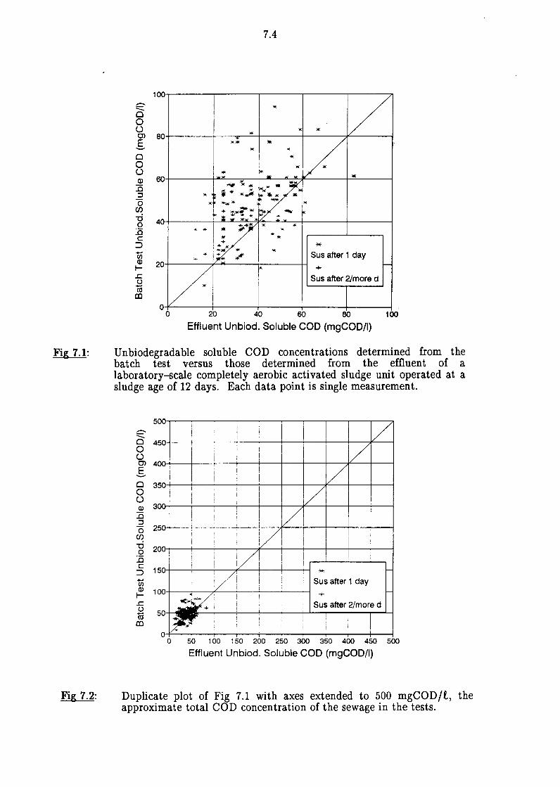
Fig 7.1:
Fig 7.2:
7.4
100 -::::::. * 0 0 (.)
* Cl 80 .s *"' "' * .
0 0 (.) Q) 60 :0 ::, 0 "' U)
"O 40 0 .. I :.0 + "'
C .. "' ::J +
* "'"' - ... "' * .. ,. .,.It' Sus after 1 day II)
* Q) 20 I- + .c Sus after 2/more d () -ca co
0 0 20 40 60 80 100
Effluent Unbiod. Soluble COD (mgCOD/1)
Unbiodegradable soluble COD concentrations determined from the batch test versus those determined from the effluent of a laboratory-scale completely aerobic activated sludge unit operated at a sludge age of 12 days. Each data point is single measurement.
-::::::. 0 450-+---+--~----i-----1---1----+--+--1--------J.'-----1 0 (.) Cl 400>-+---+--......--+---+--+---.--+--i4---1--1 .s 0 3501+--4---i-------+---+--+---l---¥---+----1--1 0 (.) Ol 300, .......... -~-......--+---+--l---¥--+--+----I--I
:0 ::,
0 250 U)
"O 200+--+--'------+---l----i---+--I-------I----I 0
:.0 5 150+---------"'-----1--+---'--' * ti Sus after 1 day ~ 100+--,-.------"-~-----~-----'--' + .c ()
nj cc
50 .. , Sus after 2/more d
50 1 00 150 200 250 300 350 400 450 500
Effluent Unbiod. Soluble COD (mgCOD/1)
Duplicate plot of Fig 7.1 with axes extended to 500 mgCOD/l, the approximate total COD concentration of the sewage in the tests.

Fig 7.3:
Fig 7.4:
7.5
24
-·.;::; Cl)
?fl. 20 - i Cl t " 0 I (.) 16 Q)
..c "' .,. ::::, "$c "' * 0 .. ,
Cl) 12 I
"O 0
:.a C
#C ::, 8 -- -1 en Q)
_$ ... f-..c ."" -. u 4 + iu Ill
0 0 4 8 12 16 20 24
Effluent Unbiod. Soluble COD (% Sti)
Data in Fig 7.1 plotted as % of the total COD (Sti)-
100 +
+ +
- 80 :::::. Cl 0 (.) O> g 60
.... Q) a. ct! a. .... 40 Q)
-= u:: +
lO s:t: 0 20
O+------,,------,----+-------+----. 0 ~ ~ 00 00 100
Glass Fibre Paper (mgCOD/1)
Unbiodegradable soluble COD concentrations derived from the batch test using 0,45µm filtration versus those using glass fibre filtration.

Fig 7.5:
Fig 7.6:
I-m 0 a: a.
7
6.5
6
~ 5.5 z <( er: Cl UJ ~ a:
5
0 4.5 LI.. Cl)
z <( a: I-
4
3.5
3 2
7.6
jsewage Batch 22 j /,. V
I / ) /
/-/-
• V Actual Results
/ -•/ True Normal Distr.
4 6 8 10 12 14
Soluble Unbio.COD(% of Sti):Batch Test
Probability plot of soluble unbiodegradable COD for batch tests on one batch of sewage from Mitchell's Plain Treatment Plant. (Sewage batch No.22).
I-m 0 a: a.
7
6.5
6
~ 5.5 z <( a: Cl UJ ~ a:
5
0 4.5 LI.. Cl)
z <( er: I-
4
3.5
3 2
j Sewage Batch 22 j I~
/
/ .. / V
11/ /' • t--
V Actual Results
-
/ True Normal Distr. ,--
4 6 8 10 12 14
Soluble Unbio.COD(% of Sti):Effluent
Probability plot of the soluble unbiodegradable COD derived from the aerobic unit effluent for one batch of sewage from Mitchell's Plain Treatment Plant. (Sewage batch No.22).

,....... -en Q)
~ ..c CJ -<tS al ........ -:.:; en -0
t< -en ::::,
en C <tS Q)
~
Fig 7.7:
7.7
10
• •• •
• 8
6
4
2
o,-------------1----.....----------------1 0 2 4 6 8 10 12
Mean Sus (% of Sti) [Aerobic Unit]
Soluble unbiodegradable COD from the batch test versus that from the aerobic unit. Each data point is the mean of a number of tests on one batch of sewage.

7.8
Table 7.'t: Mean unbiodegradable soluble COD (Sus) (as % of Sti), number of tests and standard deviation of the means for the batch tests and the aerobic unit method for the different sewage batches.
Sewage Mean Soluble Unbiodegradable COD (% of Sti) Batch Test Activated Sludge System Mean No of Std.dev. Mean No of Std.dev.
Batch Sus Tests of mean Sus Tests of mean 5 10 6 0.8 9 6 0.7 6 10 6 1.0 9 6 0.8 7 8 6 0.5 8 6 0.5 8 11 4 0.3 10 4 0.8 9 10 8 0.4 8 8 0.6 10 8 9 0.9 8 9 0.6 11 9 5 0.9 8 5 0.9 12 9 11 0.7 8 11 0.7 13 9 12 0.7 7 12 0.5 14 8 12 0.4 7 12 0.6 15 7 12 0.5 7 12 0.6 16 9 7 0.8 5 7 0.5 17 8 14 0.7 8 14 0.4 18 8 10 0.7 7 10 0.8 19 8 6 0.6 7 6 0.7 20 8 10 0.6 7 10 0.4 21 8 9 0.6 6 9 0.5 22 8 9 0.9 7 9 0.8

CHAPTER 8
EXTENSION OF THE BATCH TEST TO DETERMINE UNBIODEGRADABLE PARTICULATE AND SLOWLY BIODEGRADABLE COD FRACTIONS
8.1 INTRODUCTION
With the batch test procedure developed thus far, three of the five influent COD
fractions can be quantified, namely readily biodegradable COD, heterotroph active
biomass and unbiodegradable soluble COD, see Chapters 4, 5 and 7. The remaining
two COD fractions, unbiodegradable particulate and slowly biodegradable COD,
still need to be determined. Conventional methods to quantify these two COD
fractions involve running laboratory-scale activated sludge systems (Ekama et al.,
1986; see Chapter 3) a time-consuming and costly exercise. In this Chapter it is the
intention to explore possible options to extend the batch test procedure to provide
estimates for these two COD fractions.
8.2 BACKGROUND
At the start of the batch test procedure, the total COD is made up of the five
influent COD fractions:
Sti = Susi + Supi + Sbsi + Sbpi + ZBHi
where
Sti =influent total COD (mgCOD/t)
Susi =influent unbiodegradable soluble COD (mgCOD/t)
Supi =influent unbiodegradable particulate COD (mgCOD/t)
Sbsi =influent readily biodegradable soluble COD (mgCOD/t)
Sbpi =influent slowly biodegradable particulate COD (mgCOD/t)
ZnHt =influent heterotroph active biomass (mgCOD/t)
(8.1)
For the influent, even with Susi, Sbsi and ZBHi determined using the procedures set
out earlier, with the information available it is not possible to differentiate between
Sbpi and Supi· Furthermore, physical filtration techniques such as those set out in
Chapter 6 also canno~ separate these two fractions - since both COD fractions are
particulate, they cann::it be separated by filtration procedures.
During the course of the batch test the two unbiodegradable COD fractions (Susi

8.2
and Supi) remain unaffected by biological action. The two biodegradable COD
fractions (Sbsi and Sbpi) are utilized, consuming oxygen and generating heterotroph
active biomass (ZBH) in the process. The heterotrophic active biomass undergoes
death/decay/lysis/endogenous respiration producing ·endogenous residue (ZE) and
slowly biodegradable COD (Sbp) which is utilized in the same fashion as the influent
slowly biodegradable COD.
At the end of the batch test (after the precipitous drop in OUR), all the readily
biodegradable COD has been consumed and the total COD is made up of
(8.2)
where
e = denotes end of test
Ste =total COD concentration at end of test (mgCOD/t)
Suse =unbiodegradable soluble COD concentration at end of test (mgCOD/t)
Supe = unbiodegradable particulate COD concentration at end of test
(mgCOD/t)
Sbpe = slowly biodegradable particulate COD concentration at end of test
(mgCOD/t)
ZBHe =heterotroph active biomass COD concentration at end of test (mgCOD/t)
ZEe =endogenous residue COD concentration at end of test (mgCOD/t)
Since the unbiodegradable COD fractions remain unaffected in the test, and
unbiodegradable COD generation in the test can be considered negligible (see
Chapter 3),
(8.3)
-In Eqs (8.1) and (8.3) the parameters Susi, Sbsi, ZBHi, Sti and Ste are known from
measurement or calculation (see Chapters 4, 5 and 7), but the parameters Supi,
Sbpi, Sbpe, ZBHe and ZEe are unknown. It is evident that to quantify the unknown
parameters, additional information has to be obtained from the batch test. In this
Chapter a number of methods are developed to attempt to obtain the necessary
information. In all the methods presented, it has to be assumed that all the slowly
biodegradable COD has been consumed in the batch test, i.e. Sbpe = 0. In terms of
the death-regeneration hypothesis of Dold et al. (1980), the slowly biodegradable

8.3
COD is derived either from the influent, or is generated by the endogenous processes
(see Table 4.1, Chapter 4). For the influent slowly biodegradable COD, it will be
assumed that sufficient time has elapsed by the end of the batch test for this COD
to have been completely consumed. For the slowly biodegradable COD generated
by endogenous processes, the rate of generation is slower than the rate of utilization.
Thus, if all the influent slowly biodegradable COD has been consumed in the batch
test, then the slowly biodegradable COD generated by endogenous processes will be
used as fast as it is generated, and the residual concentration will be negligible.
Accordingly, Sbpe will be close to zero. To simplify interpretation and analysis of
the data from the batch tests, the death-regeneration approach (Dold et al., 1980)
will be replaced with the endogenous-respiration approach (Marais and Ekama,
1976). In the endogenous-respiration approach, the heterotroph active biomass
"dies" at a certain rate; of the biomass lost, the biodegradable portion gives rise
directly to oxygen utilization ( there is no substrate intermediate) and the
unbiodegradable portion to endogenous residue. Under the aerobic condit'ions
present in the batch test, both the death-regeneration and endogenous-respiration
approaches give the same nett result, i.e. same loss of heterotroph active biomass,
utilization of oxygen and generation of endogenous residue. However, the
endogenous-respiration approach allows the oxygen utilization rate to readily
separate into that for endogenous-respiration and that for heterotroph active
biomass synthesis. Also, in the endogenous respiration approach the only source of
slowly biodegradable COD in the batch test is from the influent wastewater. As
will be seen, these consequences facilitate analysis of the batch test data.
Accepting the endogenous respiration approach, then the basic assumption is that
all the influent slowly biodegradable COD has been consumed in the batch test, i.e.
Sbpe = 0. This reduces the number of unknowns to four, i.e. Supi, Sbpi, ZBHe and
ZEe· The methods developed below attempt to quantify these four unknowns.
8.3 METHOD 1: DIVISION OF OUR
In the batch test, the OUR-time plot (e.g. Fig 4.1, Chapter 4) represents the
oxygen utilized in the consumption of the two influent biodegradable COD fractions
(Sbsi and Sbpi) for heterotroph active biomass synthesis, and that utilized in
endogenous processes. ( As noted earlier in Chapter 4, there is no nitrification so
that nitrification does not exert an OUR in the batch test). If the OUR can be
divided between that for heterotroph active biomass synthesis from the influent
biodegradable COD and that for endogenous processes, then with the assumption

8.4
that all the influent biodegradable COD is consumed in the batch test, it should be
possible to derive estimates for the influent biodegradable COD. Since the influent
readily biodegradable COD (Sbsi) can be quantified (see Chapters 4 and 5), then the
difference between the biodegradable COD and Sbsi should give the influent slowly
biodegradable COD (Sbpi)· With Sbpi quantified the unbiodegradable particulate
COD (Supi) can be found by subtracting Sbpi, Sbsi, Susi and ZBHi, from the total
COD (Sti).
8.3.1 Test procedure
The batch tests were run using the procedure set out in Chapter 4; the batch tests
were run for 2 or more days in order to ensure all the influent biodegradable COD
is consumed ( a condition necessary for application of this procedure).
Comprehensive data for all batch tests are listed in Appendix A. A typical OUR
versus time profile is shown in Fig 8.1. From the graph it can be seen that the
initial period ( < 18h) corresponds to that detailed in Chapter 4, i.e. exponential
increase in OUR, precipitous drop followed by an OUR plateau then decrease. As
the batch test continues to run for a longer period ( except for a small increase at
:1: 20h) the OUR continually decreases to reach an approximately constant value
after about 60 hours. From the low OUR values at the end of the test (:1: 60 hours),
a line was back projected to the start of the test, i.e. time = 0 hours (see Fig 8.1).
This line represents the division between the OURs associated with endogenous
respiration and utilization of the biodegradable COD in the influent wastewater, i.e.
the part of the graph above the line represents the OUR due to the utilization of
influent biodegradable COD and that below the line the OUR due to endogenous
processes, as shown in Fig 8.1.
8.3.2 Data interpretation
At the end of the batch test it is assumed that all the influent biodegradable COD has
been consumed. The OUR at the end of the test therefore is the OUR due to -
endogenous respiration only. By back projecting this OUR to the start of the test
(for example see Fig 8.1), it was hoped that the measured oxygen consumption
would be divided into that for heterotroph active biomass synthesis from the
influent biodegradable COD and that for endogenous processes, as described above.
Now, for the OUR associated with heterotroph active biomass synthesis,
MOsynthesis = (1-Y zH) Sbi (8.4)

8.5
where
MO synthesis = oxygen consumed for heterotroph active biomass synthesis from
influent biodegradable COD (mgO/t)
Y ZH = heterotroph active biomass yield (mgCOD/mgCOD)
=0,666 mgCOD/mgCOD
=influent wastewater biodegradable COD concentration
(mgCOD/t)
Therefore, solving Eq (8.4) for Sbi,
= MOsynthesis/(1-Y zH) (8.5)
From Eq (8.5) if MOsynthesis is known, then Sbi can be determined; MOsynthesis is
obtained from the OUR-time profile (see Fig 8.1) as the area under the OUR-time
curve minus the oxygen consumed for endogenous processes, see Fig 8.1. With Sbi
quantified following the procedure above and with Sbsi available from the
procedures set out in Chapter 4, Sbpi can be determined as follows:
(8.6)
With Sbpi quantified, Supi can be calculated from the measured influent total COD
concentration (Sti), i.e.
Supi = sti - sbi - Susi - ZBHi (8. 7a)
Also, the fraction of the total influent COD that is unbiodegradable particulate (fup)
can be calculated:
(8.7b)
Thus, by subdividing the oxygen consumption in the batch between that for
synthesis and that for endogenous processes, the remaining two COD fractions, Sbpi
and Supi can be quantified, and hence the wastewater COD fractions completely
characterized.
8.3.3 Results
A number of batch tests were run; detailed data are listed in Appendices A and B.

8.6
For the batch tests, the results were calculated using Eqs (8.4) to (8. 7) above;
results for the tests are shown in Table 8.1 (see Table 5.1 for wastewater batch
source).
From Table 8.1 it can be seen that the values for fup are very variable, ranging from
--0,14 to +0,45. Also, four batch tests (Table 8.1, wastewater, batch No. 11,
Feb 23rd, and batch No. 13, 3rd, 7th and 9th April) gave negative values for the
unbiodegradable particulate COD in the influent; this is because the OUR due to
endogenous processes was underestimated. Furthermore, even for the same
wastewater batch the calculated fup values varied considerably; for example, for
wastewater batch No. 13, the fup varied from --0,14 to +0,39. Clearly this method
does not provide consistent, reasonable estimates for fup and was rejected for further
development.
8.3.4 Conclusions
This method to quantify the remaining two influent COD fractions did not prove
successful. The technique used to divide the measured OUR between that for
synthesis from influent biodegradable COD and that for endogenous processes
probably is not valid - the heterotroph active biomass concentration varies
considerably during the course of the batch test and therefore so will the OUR
associated with endogenous processes; in both the endogenous respiration and death
regeneration approaches, the OURs arising from these processes are directly
proportional to the heterotroph active biomass concentration. Furthermore, for this
method it has to be assumed that all the influent biodegradable COD has been
consumed by the end of the test - this assumption could not be verified.
8.4 METHOD 2: PASTEURIZATION OF INFLUENT WASTEWATER
In Method 1 above, the problem was estimation of the endogenous respiration OUR,
made .by subdividing the OUR between that for heterotroph active biomass
synthesis and endogenous respiration. It was hypothesized that if the OUR due to
endogenous respiration could be reduced to such low values that it makes a
negligible contribution to the measured OUR, then a more reliable estimate of the
OUR for heterotroph active biomass synthesis on influent biodegradable COD could
be obtained. For the batch test it can be proposed that predation will dominate the
OUR for endogenous respiration. This proposal arises from the work of Bhatla and
Gaudy (1965a,b) on BOD-time profiles in the standard BOD test. A typical
BOD-time profile is shown plotted in Fig 8.2. In the BOD test, oxygen uptake
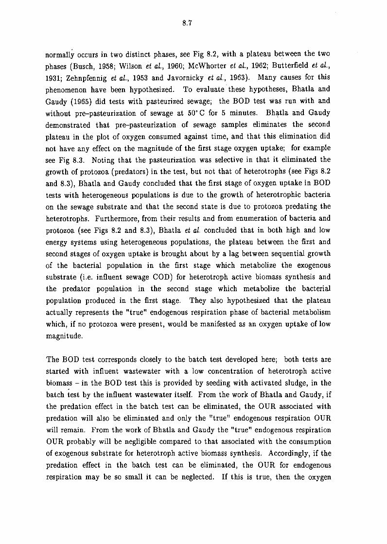
8.7
normally occurs in two distinct phases, see Fig 8.2, with a plateau between the two
phases (Busch, 1958; Wilson et al., 1960; McWhorter et al., 1962; Butterfield et al.,
1931; Zehnpfennig et al., 1953 and Javornicky et al., 1963). Many causes for this
phenomenon have been hypothesized. To evaluate· these hypotheses, Bhatla and
Gaudy (1965) did tests with pasteurized sewage; the BOD test was run with and
without pre-pasteurization of sewage at 50° C for 5 minutes. Bh~tla and Gaudy
demonstrated that pre-pasteurization of sewage samples eliminates the second
plateau in the plot of oxygen consumed against time, and that this elimination did
not have any effect on the magnitude of the first stage oxygen uptake; for example
see Fig 8.3. Noting that the pasteurization was selective in that it eliminated the
growth of protozoa (predators) in the test, but not that of heterotrophs (see Figs 8.2
and 8.3), Bhatla and Gaudy concluded that the first stage of oxygen uptake in BOD
tests with heterogeneous populations is due to the growth of heterotrophic bacteria
on the sewage substrate and that the second state is due to protozoa predating the
heterotrophs. Furthermore, from their results and from enumeration of bacteria and
protozoa (see Figs 8.2 and 8.3), Bhatla et al. concluded that in both high and low
energy systems using heterogeneous populations, the plateau between the first and
second stages of oxygen uptake is brought about by a lag between sequential growth
of the bacterial population in the first stage which metabolize the exogenous
substrate (i.e. influent sewage COD) for heterotroph active biomass synthesis and
the predator population in the second stage which metabolize the bacterial
population produced in the first stage. They also hypothesized that the plateau
actually represents the "true" endogenous respiration phase of bacterial metabolism
which, if no protozoa were present, would be manifested as an oxygen uptake of low
magnitude.
The BOD test corresponds closely to the batch test developed here; both tests are
started with influent wastewater with a low concentration of heterotroph active
biomass - in the BOD test this is provided by seeding with activated sludge, in the
batch test by the influent wastewater itself. From the work of Bhatla and Gaudy, if
the predation effect in the batch test can be eliminated, the OUR associated with
predation will also be eliminated and only the "true" endogenous respiration OUR
will remain. From the work of Bhatla and Gaudy the "true" endogenous respiration
OUR probably will be negligible compared to that associated with the consumption
of exogenous substrate for heterotroph active biomass synthesis. Accordingly, if the
predation effect in the batch test can be eliminated, the OUR for endogenous
respiration may be so small it can be neglected. If this is true, then the oxygen

8.8
consumption for heterotroph active biomass synthesis on wastewater biodegradable
COD (MOsynthesis) will simply be the area under the OUR-time profile in the batch
test. With MOsynthesis determined, Shi, Sbpi and Supi can be calculated using Eqs
(8.5), (8.6) and (8.7) respectively. ·
8.4.1 Test procedure
Bhatla and Gaudy (1965) demonstrated that selective pasteurization of sewage
samples eliminated the growth of predators in BOD type tests, see above.
Accordingly, it was decided to selectively pasteurize the wastewater samples prior to
the batch test procedure set out in Chapter 4. Selective pasteurization was achieved
by heating the wastewater to 50° C for 5 minutes, then cooling the wastewater to
20· C for the batch test - this pasteurization procedure selectively kills protozoa
(predators) and not bacteria (Bhatla and Gaudy, 1965).
8.4.2 Results
A number of these batch tests were run, all exhibited similar behavioural patterns.
Comprehensive data are listed in Appendix A. A typical OUR-time profile is shown
plotted in Fig 8.4. From Fig 8.4, the OUR-time profile with pasteurization differs
considerably from those of batch tests without pasteurization ( cf Chapter 4, Fig
4.1). For the batch tests with prior pasteurization, from the start of the batch test
the OUR follows the typical exponential increase to the peak OUR at time = ± 10h.
However, the OUR-time profile then exhibits a very much reduced precipitous drop
in OUR whereafter the OUR increases to a second peak, a feature not seen in any of
the non-pasteurized batch tests. It was hypothesized that this second OUR peak
was due to a change in the wastewater COD characteristics caused by heating the
wastewater during pasteurization; it would seem that the pasteurization step
resulted in breakdown of some of the complex organics that constitute the SBCOD
making these more easily biodegradable by the biomass. In this method, because
the precipitous drop in OUR could not be clearly identified the influent readily
biodegradable COD concentration (Sbsi) could not be quantified using the
procedures set out in Chapter 4. Because Sbsi could not be determined, Sbpi and
Supi also could not be determined, see Eq (8.6) and (8.7) respectively.
8.4.3 Conclusion
Pasteurization of the wastewater prior to the batch test to reduce the endogenous
respiration effect results in behavioural patterns that deviate considerably from
those in batch tests without prior pasteurization. Thus, this method was rejected

8.9
for further development.
8.5 METHOD 3: EXTENDED AERATION
In this method the basic assumption is that the heterotroph active biomass at the
end of the batch test is so small that it can be neglected (i.e. ZBHe = 0). If this
assumption is valid, then enough information can be obtained from t~e batch test to
quantify the remaining unknown parameters.
8.5.1 Test procedure
The test procedures set out in Chapters 4, 5 and 7 were followed, except that the
length of the batch was extended to at least 3 days. After 3 days it was hoped that
the heterotroph active biomass concentration in the batch test would be minimal.
A number of batch tests were run. Comprehensive data are listed in Appendices A
and B. A typical OUR-time plot for the extended batch test is shown in Fig 8.5.
Even with extended aeration, an increase in nitrate was not detected in any of the
batch tests indicating that no nitrification occurred in the batch test, i.e. an absence
of autotrophic biomass.
8.5.2 Data interpretation
The area under the OUR-time curve is the mass of oxygen consumed (MOc)- In the
absence of nitrification the MOc is due to oxygen consumption for heterotroph
active biomass synthesis on the influent biodegradable COD (MOsynthesis) and for
endogenous respiration (MOe), i.e.
MOc = MOsynthesis + MOe (8.8)
Assuming that all the influent biodegradable COD (Shi) is consumed in the batch
test, then
. MOsynthesis = (1-Y zH) Sbi (8.9)
The heterotroph active biomass that is produced in this growth process ( Ll ZBH) is
(8.10)
From the assumption that the heterotroph active biomass concentration at the end
of the test is negligible, all the heterotroph active biomass in the influent (ZBHi) or

8.10
generated in the growth process (~ZnH) must be endogenously respired. Accepting
that a fraction (f) of the heterotroph active biomass is unbiodegradable endogenous
residue (WRC, 1984), then a fraction (1-f) must contribute to the oxygen
consumption in endogenous respiration, i.e.
MOe = (1-f) ~ZBH + (1-f) ZBHi
= (1-f) Y ZH Sbi + (1-f) ZBHi (8.11)
Substituting Eqs (8.9) and (8.11) into Eq (8.8)
MOc = (1-Y zH) Sbi + (1-f) Y ZH Sbi + (1-f) ZBHi (8.12)
Solving Eq (8.12) for Sbi
(8.13)
In Eq (8.13), MOc and ZBHi are available from measurements made in the batch
test ( see Chapter 4). Values have to be assumed for the constants Y ZH and f:
Y ZH = 0,666 mg COD /mgCOD
f = 0,2 mgCOD /mgCOD (WRC, 1984)
Thus, Sbi can be determined based on the assumption for this extended aeration
batch test, namely that the heterotroph active biomass concentration at the end of
the test is negligible (i.e. ZnHe = 0). From Sbi and Sbsi, Sbpi can be determined
~
With Sbpi quantified, Supi can be determined
Supi = Sti - Sbpi - Susi - Sbsi - ZBHi
and
fup = Supi/Sti
8.5.3 Results
(8.14)
(8.15)
(8.16)
A number of the extended aeration batch tests were run using raw (unsettled)

8.11
municipal wastewater obtained from Mitchell's Plain (Cape Town). Comprehensive
data are listed in Appendices A and B. A typical OUR-time profile is given in Fig
8.5. Using the procedures detailed in Chapters 4 and 7 and those set out above, the
influent wastewater COD fractions for the different hatch tests were quantified and
are listed in Table 8.2. From Table 8.2, values for fup using this method show some
consistency; standard deviation of the mean (SDm) = 0,07, 0,05 and ,0,03 for sewage
batches 12, 13 and 14 respectively. However, the values are considerably higher
(mean fup = 0,36 to 0,49) than expected for a typical South African raw municipal
wastewater (fup : 0,13, WRC, 1984). In examining the procedure for calculation for
Supi, it is evident that the main assumption is that the heterotroph active biomass
concentration at the end of the batch test is negligible. If, contrary to this
assumption, appreciable heterotroph active biomass is present at the end of the
batch test, then the calculation procedure will incorporate the heterotroph active
biomass in Supi leading to overestimation of this value and the associated fup·
Clearly, the heterotroph active biomass concentration at the end of the batch test is
not negligible and this causes Supi to be overestimated.
8.5.4 Conclusion
From this study it can be concluded that the basic assumption, that after 3 days of
aeration in the batch test the quantity of heterotroph active biomass is so small that
it can be neglected, is not valid. Therefore, the method for determining Sbpi and
Supi based on this assumption will not be successful. In any event, having to run
the batch test for longer than 3 days would greatly reduce its attractiveness for
practical application.
8.6 METHOD 4: OUR AT THE END OF THE BATCH TEST
From METHOD 3 above it is apparent that appreciable heterotroph active biomass
is present after 3 days of running the batch test. If it is possible to quantify this
heterotroph active biomass, then sufficient information should be available from the
batch test to quantify the remaining unknown parameters, provided it is assumed
that all the influent biodegradable COD has been consumed. In this method it is
proposed to use the absolute value of the OUR at the end of the batch test to
quantify the heterotroph active biomass concentration at the end of the test.
8.6.1 Test procedure
The data from METHOD 3 above was used for METHOD 4.

8.12
8.6.2 Data interpretation Assuming that all the influent biodegradable COD {Sbi) has been consumed by the
end of the test, then the OUR at the end of the test is due to endogenous
respiration only. The endogenous respiration OUR (Oe) can be formulated as
(WRC, 1984)
=endogenous respiration OUR at time t (mgO/t/h)
= net specific endogenous mass loss rate
= 0,24/d
=heterotroph active biomass at time t (mgCOD/t)
At the end of the batch test t=e, solving Eq (8.17) for ZBHe gives
{8.17)
{8.18)
Thus, from Eq {8.18) if the OUR at the end of that batch test is known and it is
assumed that this OUR is due to endogenous respiration only, OUR = Oee (i.e. all
the influent biodegradable COD has been consumed), the heterotroph active biomass
concentration at the end of the batch test (ZBHe) can be calculated. What is still
required is to determine the influent biodegradable COD (Shi) concentration.
Conducting a mass balance around the heterotroph active biomass (ZBH) over the
batch test: At the start of the batch test, ZBH is present in the influent wastewater
(ZBHi); during the course of the batch test ZBH is synthesized from the
biodegradable COD [ZBH(synthesized)] and is endogenously respired; at the end of
the batch test some ZBH remains (ZBHe). From the mass balance, the ZBH lost in
endoge~ous respiration [ZBH{lost)] is given by
ZBH(lost) = ZBHi - ZBHe + ZBH(synthesized) (8.19)
Now, from the assumption that all the biodegradable COD (Sbi) is consumed in the
batch test,
ZBH(synthesized) = Y ZH Sbi (8.20)
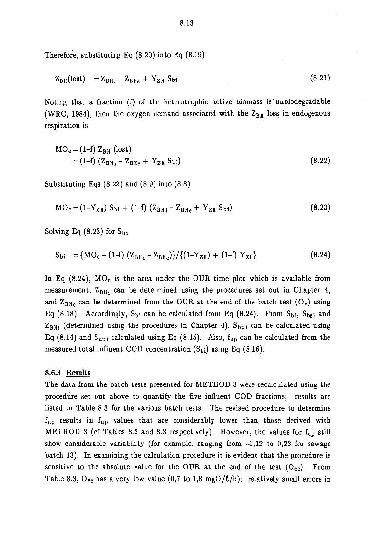
8.13
Therefore, substituting Eq (8.20) into Eq (8.19)
Z8H(lost) = ZBHi - ZeHe + Y ZH Sbi (8.21)
Noting that a fraction (f) of the heterotrophic active biomass is unbiodegradable
(WRC, 1984), then the oxygen demand associated with the ZeH los~ in endogenous
respiration is
MOe=(l-f) Z8 H (lost)
= (1-f) (ZBHi - ZBHe + Y ZH Shi) (8.22)
Substituting Eqs (8.22) and (8.9) into (8.8)
MOc = (1-Y zH) Sbi + (1-f) (ZBHi - ZeHe + Y ZH Sbi) (8.23)
Solving Eq (8.23) for Shi
Sbi = {MOc - (1-f) (ZBHi - ZeHe)}/{(l-YzH) + (1-f) YzH} (8.24)
In Eq (8.24), MOc is the area under the OUR-time plot which is available from
measurement, ZBHi can be determined using the procedures set out in Chapter 4,
and ZeHe can be determined from the OUR at the end of the batch test (Oe) using
Eq (8.18). Accordingly, Sbi can be calculated from Eq (8.24). From Sbi, Sbsi and
ZBHi ( determined using the procedures in Chapter 4), Sbpi can be calculated using
Eq (8.14) and Supi calculated using Eq (8.15). Also, fup can be calculated from the
measured total influent COD concentration (Sti) using Eq (8.16).
8.6.3 Results
The data from the batch tests presented for METHOD 3 were recalculated using the
procedure set out above to quantify the five influent COD fractions; results are
listed in Table 8.3 for the various batch tests. The revised procedure to determine
fup results in fup values that are considerably lower than those derived with
METHOD 3 ( cf Tables 8.2 and 8.3 respectively). However, the values for fup still
show considerable variability (for example, ranging from --0,12 to 0,23 for sewage
batch 13). In examining the calculation procedure it is evident that the procedure is
sensitive to the absolute value for the OUR at the end of the test (Oee). From
Table 8.3, Oee has a very low value (0, 7 to 1,8 mgO /t/h); relatively small errors in

8.14
the mea'surement of Oee (± 0,5 mgO/t/h) are significant compared to the absolute
value, and cause significant errors in the calculated fup· To illustrate the sensitivity
of the fup value calculated using the procedure above to errors in the measurement
of Oee, a theoretical plot of fup versus Oee is shown in Fig 8.6; a relatively small
absolute error in the measurement of Oee gives rise to a large error in the calculated
fup value.
8.6.4 Conclusion
Although this method provides estimates for fup that are an improvement over the
previous methods, the measured OUR at the end of the batch test cannot be
successfully used to determine heterotroph active biomass at the end of the test,
thereby to calculate unbiodegradable particulate and slowly biodegradable COD.
The proposed method is too sensitive to small absolute errors (± 0,5 mgO/t/h) in
the measurement of the OUR because the value for the OUR at the end of the test
is small ( < 2,0 mgO/t/h). This sensitivity results in fup values that show
considerable variability.
8. 7 METHOD 5: ACETATE ADDITION
In METHOD 4 it was shown that if the heterotroph active biomass at the end of
the batch test can be quantified, then the five influent COD fractions can be
calculated using the data available from the batch test. In METHOD 4 it was
attempted to quantify this heterotroph active biomass from the measured absolute
OUR value at the end of the batch test; this technique was not successful due to
the sensitivity of the calculation procedure to relatively small absolute errors in the
measured OUR. It was decided to explore other techniques to quantify the
heterotroph active biomass remaining at the end of the batch test.
In the batch test, the heterotroph active biomass at the start of the test can be
quantified from the exponential increase in OUR caused by the growth of
heterotrophs on the readily biodegradable COD (RBCOD) present in the influent
wastewater (see Chapter 4). It was proposed to duplicate this technique at the end
of the batch test by adding the artificial RBCOD sodium acetate. On addition of
the sodium acetate, the OUR should show an exponential increase as it does at the
start of the batch test. Using the procedures developed in Chapter 4, the
heterotroph active biomass concentration at the time of addition of the sodium
acetate can be determined from the exponential increase in OUR. With the
heterotroph active biomass concentration determined, Sbi, Sbpi and Supi ( and fup)

8.15
can be calculated using the procedures set out in METHOD 4 above.
8.7.1 Biomass behaviour with acetate addition - preliminary investigation
With addition of an artificial substrate (in this case sodium acetate), the possibility
exists that the biomass behaviour will deviate from that with wastewater substrate.
Accordingly, it was decided to assess in some manner whethe.r the biomass
behaviour with acetate addition conforms to that with wastewater, before the full
batch test procedure was implemented.
To evaluate the biomass behaviour with acetate addition, the normal batch test
procedure as set out in Chapters 4, 5 and 7 was followed until after the precipitous
drop in OUR. The batch test was continued for about 2 hours whereafter sodium
acetate was added to the batch test at a concentration of 102 mgCOD/t batch
reactor taking due account of the reduced batch volume because of sampling. The
batch test was then continued for a further 12 hours following the standard
procedure set out in Chapter 4. This procedure was repeated for 11 batch tests.
Comprehensive data are listed in Appendix A and B; a typical OUR-time profile is
shown plotted in Fig 8. 7a.
From Fig 8. 7a, following the addition of sodium acetate there is a step increase in
the OUR, whereafter the OUR shows an exponential increase. The exponential
increase in OUR conforms to the exponential increase at the beginning of the test,
therefore, qualitatively it would seem that the analytical procedures set out in
Chapter 4 can be used to estimate the heterotroph active biomass present at the
time of sodium acetate addition.
To provide some quantitative assessment of whether the biomass behaviour
conforms to that with wastewater, from the area under the OUR-time curve due to
acetate consumption, Area A, Fig 8. 7a, the heterotroph active biomass yield on
acetate can be calculated:
J OUR (acetate) dt
YzH =1--------COD (acetate)
where
= heterotroph active biomass yield on acetate
(8.25a)

8.16
(mgCOD/mgCOD)
J OUR (acetate) dt = area under OUR-time curve due to acetate consumption,
Area A, Fig 8.7a (mgO/t) .
COD (acetate) = known COD concentration of added sodium acetate
(mgCOD/t)
For the batch tests, the data and calculated heterotroph yield (Y zH) are listed in
Table 8.4; the mean yield for the 11 batch tests was 0,646 mgCOD /mgCOD with
standard deviation of the mean of 0,007. Thus, the yield with sodium acetate (0,646
mgCOD/mgCOD) is very close to that measured with wastewater (0,666 mgCOD/
mgCOD; Dold and Marais 1986). It would appear that the behaviour of the
heterotrophs with acetate as substrate does conform to the behaviour with
wastewater. Furthermore, that the yield obtained with the acetate closely equals
the "standard" value for the yield quoted in the literature ( e.g. WRC, 1984; Dold
and Marais 1986), would lend support to using the "standard" value of YzH = 0,666
mgCOD /mgCOD in all other calculations.
8. 7.2 Test procedure
Having ascertained that the heterotroph biomass behaviour with acetate as
substrate can be expected to be similar to that with wastewater as substrate, the
full batch test procedure could be implemented. The normal batch test procedure as
set out in Chapters 4, 5 and 7 was followed for 1 or 2 days. Thereafter, a sample
was drawn from the batch test and total COD and flocculated-filtered COD (see
Chapter 6) determined. Sodium acetate was then added to the batch test at a
concentration of 102 mgCOD/t batch reactor taking due account of the reduced
batch volume because of sampling. The batch test was then continued for a further
12 hours following the standard procedures set out in Chapter 4. The procedure was
repeated for 10 batch tests. Comprehensive data for the batch tests are listed in
Appenclix A and B. Typical OUR-time profiles are shown plotted in Fig
8.7b and c.
8. 7 .3 Data evaluation
Following the addition of sodium acetate there is a step increase in the OUR,
whereafter the OUR shows an exponential increase, see Fig 8. 7b and c. The
exponential increase in the OUR-time profile can be analyzed to determine the
heterotroph active biomass concentration as set out in Chapter 4 - the time of
sodium acetate addition is set to zero, the OUR is plotted tn OUR versus time and
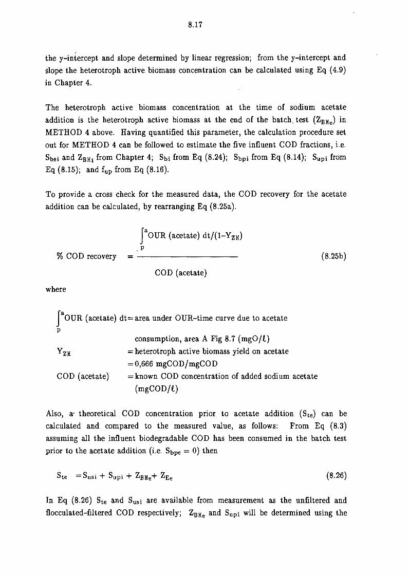
8.17
the y-intercept and slope determined by linear regression; from the y-intercept and
slope the heterotroph active biomass concentration can be calculated using Eq ( 4.9)
in Chapter 4.
The heterotroph active biomass concentration at the time of sodium acetate
addition is the heterotroph active biomass at the end of the batch, test (ZBHe) in
METHOD 4 above. Having quantified this parameter, the calculation procedure set
out for METHOD 4 can be followed to estimate the five influent COD fractions, i.e.
Sbsi and ZBHi from Chapter 4; Sbi from Eq (8.24); Sbpi from Eq (8.14); Supi from
Eq (8.15); and fup from Eq (8.16).
To provide a cross check for the measured data, the COD recovery for the acetate
addition can be calculated, by rearranging Eq (8.25a).
% COD recovery
where
JaoUR (acetate) dt/(l-YzH) p
- ----------
COD (acetate)
JaoUR ( acetate) dt= area under OUR-time curve due to acetate p
COD (acetate)
consumption, area A Fig 8.7 (mgO/t)
= heterotroph active biomass yield on acetate
=0,666 mgCOD/mgCOD
= known COD concentration of added sodium acetate
(mgCOD/t)
(8.25b)
Also, a; theoretical COD concentration prior to acetate addition (Ste) can be
calculated and compared to the measured value, as follows: From Eq (8.3) assuming all the influent biodegradable COD has been consumed in the batch test
prior to the acetate addition (i.e. Sbpe = 0) then
(8.26)
In Eq (8.26) Ste and Susi are available from measurement as the unfiltered and
flocculated-filtered COD respectively; ZBHe and Supi will be determined using the

8.18
procedure set out above. An equation for ZEe can be formulated as follows: Noting
that a fraction (f) of ZnH is unbiodegradable and generates ZE in endogenous
respiration (WRC, 1984), then the amount of ZE generated in the batch test (~ZE)
is given by
(8.27a)
Assuming that the amount of ZE at the start of the batch test is negligible ( a
reasonable assumption because any ZE present will be lumped into Supi), then
(8.27b)
Substituting Eq (8.27a) and (8.21) into (8.27b)
(8.28)
Thus, in Eq (8.26) Susi, Supi, ZnHe and ZEe can be calculated from the batch test
data using the procedures set out above. The sum of these parameters will give a
theoretical total COD concentration immediately prior to the acetate addition (Ste)
This theoretical value can be compared to the measured value, to provide a cross
check on the reliability of the data.
8. 7.4 Results
Comprehensive data for the batch tests are listed in Appendices A and B. For the
ten batch tests the calculated values for the various parameters are listed in Table
8.5a. COD recoveries for the acetate addition, calculated using Eq (8.25b) are listed
in Table 8.5b; generally COD recoveries were good (mean % COD recovery = 99%;
standard deviation of mean = 4,0%), lending support to the reliability of the
measurements. Also, the good COD recoveries indicate that the value for the
heterotroph yield used in Eq (8.25b) (Y ZH = 0,666 mgCOD/mgCOD) is acceptable -
this provides support for using this value for the yield in the other calculations.
However, from Table 8.5a calculated values for fup varied considerably (fup = 0,05
to 0,49) and were considerably higher (mean fup = 0,28) than expected (fup = :t:
0,13; WRC, 1984), and higher than the values estimated using METHOD 4 above
(see Table 8.3a). Furthermore, the calculated theoretical COD concentrations (Ste)
prior to acetate addition usually were significantly higher than those measured
(CODend) (see Table 8.5). It would appear that this method underestimates the

8.19
heterotroph active biomass present when the acetate is added. This in turn leads to
an overestimation of the fup value and accordingly, the total COD concentration at
the end of the test. It can be hypothesized that in the batch test there was selective
utilization of the artificial substrate acetate, that is, ·not all the heterotroph active
mass present in the batch test had the ability to utilize acetate - the heterotrophic
active biomass determined from the exponential increase in OUR fqllowing acetate
addition will include only those heterotrophs that can utilize the acetate. This
hypothesis would appear to be supported by an apparent lag phase following acetate
addition, see Fig 8.8a and c. Probably some acclimatization to the acetate substrate
is required, a requirement that cannot be accommodated within the structure of the
batch test method.
8. 7.5 Conclusions
The method proposed to determine heterotroph active biomass at the end of the
batch test by adding the artificial substrate acetate underestimates the heterotroph
active biomass concentration, leading to an overestimation of the unbiodegradable
particulate COD. It would appear that not all the heterotroph active biomass
present in the batch test has the ability to metabolize acetate - some kind of
acclimatization to the acetate is required. Acclimatization of the heterotrophs in
the batch test to acetate can not be accommodated in the calculation procedures -
this method was rejected for further development.
8.8 METHOD 6: RAW SEWAGE FILTRATE ADDITION
In METHOD 4, a procedure was developed whereby the values for the five influent
COD fractions can be calculated provided that the heterotroph active biomass at
the end of the batch test can be quantified. In an attempt to quantify the
heterotroph active biomass at the end of the batch test, in METHOD 4 the OUR at
the end of the batch test was used and in METHOD 5 sodium acetate was added.
The techniques in METHOD 4 and METHOD 5 used for this quantification did not
prove successful. With METHOD 4, the proposed procedure proved too sensitive to
small absolute errors in the measurement of the OUR. With METHOD 5, the
artificial substrate acetate appeared to be used selectively by some of the bacteria
leading to an underestimation of the heterotroph active biomass. To overcome the
problem of selective utilization, it was decided to replace the addition of acetate at
the end of the batch test with the addition of wastewater. To eliminate addition of
heterotroph active biomass with the wastewater, the wastewater was first filtered
through 0,45µm filters and the filtrate added to the batch test. To confirm that the

8.20
0,45µm filtrate did not contain heterotroph active biomass, the filtrate itself was
subjected to a separate batch test following the procedure set out in Chapter 4 - the
filtrate exhibited no measurable OUR indicating an absence of heterotroph active
biomass.
8.8.1 Test procedure
The batch test procedure as set out in Chapters 4, 5 and 7 was followed for 2 days.
Raw (unsettled) municipal wastewater from the same source (Mitchell's Plain) and
batch used to start the batch test was filtered through glass fibre filters (Whatman's
GF /C) and the filtrate refiltered through 0,45µm (Millipore HVLP); the
prefiltration with glass fibres is to reduce blinding of the 0,45µm filters.
After 2 days of the batch test, H. of the batch reactor mixed liquor was drawn off
and analyzed for total COD and flocculation-filtration COD (see Chapter 6). The
H drawn off was replaced with H of wastewater 0,45µm filtrate. The batch test
was then run for a further 12h or until after the second precipitous drop in OUR. A
number of batch tests were run. For detailed data see Appendices A and B. A
typical OUR-time profile is shown in Fig 8.8a.
8.8.2 Data interpretation
Following addition of the wastewater 0,45µm filtrate, the OUR-time profile ( e.g.
Fig 8.8a) was analyzed using the procedures set out in Chapter 4, to determine
heterotroph active biomass immediately after filtrate addition - the time of filtered
wastewater addition is set to zero, the OUR plotted ln OUR versus time and the
y-intercept and slope determined by linear regression; from the y-intercept and
slope the heterotroph active biomass concentration immediately after filtered
wastewater addition could be calculated using Eq ( 4.9) in Chapter 4. To convert
this value to that immediately prior to wastewater filtrate addition (i.e. the
heterotrophic active biomass concentration at the "end" of the batch test), the
dilution effect of adding the filtrate had to be taken into account as follows:
Va ZBH =ZBH • -
P a V p
where
(8.29)
ZBHp = heterotroph active biomass immediately prior to filtrate addition
(mgCOD/l)

8.21
ZBHa = heterotroph active biomass immediately after filtrate addition
(mgCOD/t), i.e. that determined from OUR-time profile after filtrate
addition
Va = batch reactor volume after filtrate addition ( t)
VP = batch reactor volume prior to filtrate addition ( t)
Having determined ZBHp, this serves as the heterotroph active biomass at the end of
the batch test (ZBHe) and the calculation procedures set out for METHOD 4 can be
followed to estimate the five influent COD fractions, i.e. Sbsi and ZBHi from
Chapter 4; Shi from Eq (8.24); Sbpi from Eq (8.14); Supi from Eq (8.15); and fup
from Eq (8.16).
8.8.3 Improvements to test procedure
Difficulties were experienced in filtering the raw wastewater through 0,45µm filters;
even with prefiltration through the glass fibre filters, the 0,45µm filters were rapidly
blinded so that at least 10 filter papers had to be used to filter H of wastewater,
making the filtration arduous and expensive. To resolve this problem it was
proposed to flocculate the wastewater by addition of aluminium sulphate prior to
0,45µm filtration. The flocculation procedure and dosages set out in Chapter 6 were
followed. Preflocculation reduced blinding of 0,45µm filters considerably. To test
whether residual aluminium, if any, would affect the behavioural patterns in the
batch test, two parallel tests were run with addition of unflocculated 0,45µm filtrate
to one batch and preflocculated 0,45µm filtrate to the other. The OUR-time
profiles for the two tests are compared in Fig 8.8a and b; no significant difference is
evident so that flocculation prior to filtration was adopted as a standard procedure.
To further reduce filtration costs, it was proposed that from the observations in
Chapter 6, the 0,45µm filter be replaced by glass fibre filters (in Chapter 6 it was
shown that with preflocculation 0,45µm and glass fibre filters gave near identical
filtrate COD concentrations). For the two filter papers, the COD concentrations of
both filtrates were identical, and starting batch tests with the two filtrates only
indicated no OUR - heterotroph active biomass was not present in either filtrate.
To check that the response induced by the preflocculated 0,45µm and glass fibre
filtrates was the same, two batch tests were run in parallel, one with addition of
preflocculated 0,45µm filtrate and the other with preflocculated glass fibre filtrate.
The OUR-time profiles using the two filter paper filtrates are shown in Fig 8.9a and
b; no significant difference between these two profiles is evident. Accordingly, for
the batch tests raw municipal wastewater was flocculated by addition of aluminium

8.22
sulphate· and then filtered through glass fibre filter papers - the filtrate was added
to the batch test after 2 days, following the procedures set out above.
8.8.4 Results
Comprehensive data for the batch tests are listed in Appendices A and B. A typical
OUR-time profile for one batch test is shown plotted in Fig 8.9a. , Following the
procedure set out above, data calculated for the batch tests are listed in Table 8.6.
For each batch of wastewater, the mean f up and standard deviations of the means
were determined, see Table 8.8. From Table 8.8, the mean values for fup for the
different wastewater batches (0,08 to 0,23) are considerably lower than those
calculated from the batch tests with acetate addition, (mean fup = 0,28, see Table
8.5) - it would appear that the problem of acclimatization with acetate addition has
been overcome by adding filtered wastewater. However, for the same wastewater
batch the fup values still exhibit considerable variability; for example, from Table
8.8 for wastewater batch 17, fup varies from 0,03 to 0,43. To explain this variability
it was hypothesized that perhaps the basic assumption in this batch test, that all
the influent biodegradable COD has been consumed prior to addition of the
wastewater preflocculated filtrate, was not valid. Accordingly, it was decided to
repeat the batch test, but to run the batch test for a longer period before adding the
wastewater filtrate.
A number of batch tests were run for 2, 3 and 4 days, see Table 8.7.
Comprehensive data are listed in Appendices A and B. Following the procedures set
out above, data calculated for the batch tests are listed in Table 8. 7. Two
wastewater batches were tested, Batch Nos. 21 and 23, see Table 8. 7. For Batch
No. 21, the batch tests were run for either 2 or 3 days prior to addition of
wastewater preflocculated filtrate. For Batch No. 23, two batch tests were run in
parallel for 3 and 4 days respectively ( on 25 and 28 0 cto ber, see Table 8. 7) prior to
addition, and three batch tests were run in parallel for 2, 3 and 4 days respectively
prior to addition (on 3 November, see Table 8.7). OUR-time profiles for the three
batch tests run in parallel for 2, 3 and 4 days are shown in Fig 8.10a, b and c
respectively.
Comparing the fup values derived for the different batch tests (see Table 8. 7), it
would appear that the effect of increasing the duration of the batch test from 2 to 3
to 4 days does not influence the estimate for fup consistently - for some tests the fup
decreases (e.g. 3rd Nov.) and for others it increases (e.g. 28th Oct.).

8.23
Accepting that increasing the duration of the batch test above 2 days does
consistently influence the estimate for Sbpi and Sbupi ( and fup), the mean fup and
standard deviations of the means for wastewater batch Nos. 21 and 23 were
determined and are listed also in Table 8.8. From T·able 8.8 the range of fup mean
values derived from the various batch tests (0,08 to 0,23) compare reasonably with
the expected values (:1::0,13). Furthermore, comparing the theoretical total COD
concentration at the end of the test [Eq (8.26)] with the measured values (see
Tables 8.6 and 8.7, and Fig 8.11), there is close correlation indicating that there is
consistency between the calculated and measured data. Thus, this method does
appear to hold promise, but requires more intensive evaluation.
8.8.5 Conclusion
It would appear that this method may provide a reasonable estimate for the five
influent COD fractions. The batch test method is relatively simple compared to
existing methods and does not require mixed liquor acclimatized to the wastewater,
nor that a laboratory-scale system be operated - both are requirements of existing
methods. As with previous methods, the batch test method does require an
uncompromising vigilance in operation to ensure measured data are reliable. This
batch test method will have to be evaluated by comparing the estimates derived for
fup with those from conventional methods.
8.9 CONCLUSION
In this Chapter it has been attempted to extend the batch test to provide estimates
of the unbiodegradable particulate and slowly biodegradable COD fractions. A
number of methods have been proposed and evaluated through trial and error, and
the less promising rejected. One proposed method appears to hold promise, that in
which preflocculated glass fibre filtered wastewater is added after 2 days. Values for
the influent unbiodegradable particulate COD fraction (fup) derived with this
method need to be evaluated, by comparing the results with those from conventional
methods.

40
-r-~
~--r--~
~-r-~
~-r-~
~--r-~
~-,---~
~-----,-~
~~
35
4 ............
............. '.*
'... .
~ *
·i ····
········
········
········
········
········
·+···-·
········
··-·····
········
·······"
·····-··
+··-···
····-···
......
........
........
........
........
........
........
........
........
........
........
........
...... +
········
·····
········
········
········
·-··t· ..
······--
········
········
········
········
-·······
······I
30-+-
-·-·-··-
~······-
··········
·········i
··········
··········
··········
...... ··
······
······
······
+·-··
······
······
······
······
--····
····-·
······
···l···
······
··-·--
·-·-··
-·---·
·····+
-·---·
··--·-
······
······
··-···
-·····
·t····
·····-
······
····-·
······
·--···
······
······
·+···
··-···
·-··-·
··-···
·---··
·-····
-~
~ *
--t
* ~
25
···-··
~.---
-····-
···--+
·-····
·---··
······
.......
..........
..........
.. , .. _
.........
. __
__
__
.,_ .....
...... --
............
-......
...... _,.
__
__
__
__
....,. _
__
__
__
__
·-•·
·
::::::::::
. 0 O
> E
..........
a:
::J
0
* *
20-+
-·t--
·---
--··-·
--·--·--
·----···
-····-
-·-·-
·---
---·
··--
+--
----
··-·
·---
-+-·
-···
-···
····
--··
·+--
·-··
···-
···-
----
,
~
Bio
deg
rad
able
CO
D O
UR
1
5-l··
··--*
---·
--·-
-...
-······
·•·-·-
········
·-···-
···-····
········
···+-··
·-·····
·-··-·
····-·-
········
········
·•·····
·-·····
······-
···-····
·······-
·-·-··
····
- ~ 1 or
* ·--· -
-·------·-
·-------
-··-·---·-·
-·· ----
-----··
··-+
--··
--·-
-__
__ .... ·-
·-·-
··--
---
~
En
do
gen
ou
s O
UR
5
·---
----
-*-
---·
-···-
-···-
+-·-
·-·-
-···-
~
o~
----+
----------+
------+
---------i-
------1
0
10
20
30
4
0
Tim
e (h
ou
rs)
50
60
Fig
8.1
: O
UR
-tim
e pl
ot f
or
an
aero
bic
batc
h te
st r
un f
or
an e
xten
ded
peri
od
show
ing
the
divi
sion
of
the
area
und
er t
he O
UR
gra
ph
acco
rdin
g to
M
ET
HO
D 1
.
70
00
~
ij::,,
.

111t 250 ..... 0
E -w ::.:: ;: 200 Q. :>
o' C w
150 t-< ..J :> ~ :> u (.)
100 ci
50
0 0
Fig 8.2:
25
8.25
I
o2u~9
I I I
I
I I
SUBSTRATE - 500 W'IO/J GLUCOSE --TEMPERATURE - Z !5°C.
I I i I I I
50 75 100 TIME. HOURS
-E ..... B ..
7
6
5
Cl u
er 0 N 0 t-0 c:: Q.
c:: 0 er c:: w t-u er a:,
c:: w
4 a:, ~ :> z C,
35
2
I 125
BOD, bacteria and protozoa counts during a WARBURG study with non-pasteurized sewage seed used for the BOD test determination. (From Bha.tla et al., 1965).

8.26
9 350 ·-----. ·-- - -·-· --
~ -- y BACTERIA ,, .. ---/ --.--
300 "'t._• y -----.z
8 I I 11 y ,,
250 I Oz UPTAKE I I 1 .,c
I / E Cllt ..... ..... I • "' I E • w 200 I"' u
-::.:: I < <
I 6 c::: I- w Q.. I-::, u N I <
0 150 I a:l
I er 0 w ~ I a:l I- I
5 ~ < ::, ..J z ::, ~ 100 --- -------- (!) ::, 0 u SUBSTRATE - soo mo/ .l GLUCOSE -J -u
TEMPERATURE - 2 S 0 c. <
4 !50
o~-~-------------------13
Fig 8.3:
0 25 50 75 100 12!5 TIME, HOURS
BOD and bacteria count during a WARBURG study with pasteurized sewage seed used for the BOD test determination. (From Bhatia et al., 1965).

1s..
...-
--..
...-
~~
.------.~
---r---~
-~
~~
-~
--..
...-
~-..
--~
--,
1 4 -+
-···---
·---.. -
---·-·
-+, .. -
..............
. _ .......
.. -........ ,
...... -.. --
.... ,-,-·-
-·-·-.. -~
,--·-.. -
..... -.-
... -... -+
,-·--·
--·-·-
---..
* ~
, *
--.. -.. -
·-.. --·-
--__
.. _______
.:__ __
-·* .. -
·-.. --,
L, .. _
____
_ .. __
12
-t--
.. ·-·--
--.. --·
-+· .. ·-
·-·-·-..
--........
+ .. -· ..
---·· .. ·-
·-+·
t ,t-
~ ,#
"
~'
* *
€ 1 o+
--.. -----
-.. ·+·--...
..... -..... _
......... j .. -.
......... -...
. -·--·-l .
. --.-· ....
--·-·-·+
~ ----··-'····
........... ·-·--.. --.~
-.... -............... -·-
-+---
---...... _
. ____
, .. ___ ,,
______
........ _
...........
-.----
-·---·
--..
:::::::.
0 0)
E - a: :::>
0
*IE
8-+
---·
·---
.. +--
·-·-
-·--
-... , ..
........
....... -
-......
---..
---·
-· .. •
-··--
·--·--
-.......
..... -·
-+;.
.'-·
----
.. ---
-•--
---·
--·-
"--
--
* * * s+
--
·--+
---7
--•-
----
-·
·---
--+
''l*
"
41-
-r--
·-·-r
-- **
* *
*' ;>l
l!IE;
* --
----
----
·-•·-
----
+--
'*** *
2-t·-
·-.. ·-
----
.... ·--t-
---·-
--* .
.... I .... -
....... _
. __
_ ....
____
,,,_ .. , ..
...... ,,, _
_ .
***
--·---
.... ·----
·+ .. ,-
... -.......
. , __ ......
........... \
.... -·-
·-.... -
--·---
·
* *
O+
---+
---+
---~
----+
---+
----+
----+
---+
---+
------,
0 2
4 6
8 1
0
12
14
16
1
8
20
Tim
e (h
ou
rs)
Fig
8.4
: O
UR
-tim
e pl
ot f
or a
n ae
robi
c ba
tch
test
wit
h pa
steu
rize
d se
wag
e.
00
~
-.:,

8.28
40
35
30
-..c 25 -------1 RBCOD oxygen uptake 1-+----+-----+-----i -::::::::. 0 C)
.s er: ::::> 0
Fig 8.5:
Q 0 (.)
20
15
10
5
0 0
0.15
0.1
0.05
0
C> -0.05 E -0 0 (.) C)
.s -0.1
-0.15
§- -0.2 -'-0.25
-0.3
-0.35
Fig 8.6:
10
oxygen uptake
I ,1
Endogenous oxygen uptake
20 30 40
Time (hours) 50 60 70
OUR-time plot for an aerobic batch test run for an extended period showing the division of the OUR area into the different OUR uptakes for the various COD utilizations.
""-._
~ I"-~ ~ ~ ~
"'-..,_
~ "
' ~ " ~
I
~ I I I
I ~ I
!~
0 0.2 0.4 0.6 0.8 1 1.2 1.4 1.6 1.8 2
OUR at the end of test (mg0/1/h)
Theoretical variation of unbiodegradable particulate COD fraction (fup) with variation in the absolute value of the OUR at the end of the batch test (Oee),

-.c -::::::::. 0 C)
E. a: ::::> 0
30
25
20
-*'#'" ~ * *
15
~ +
"" 10 ;#
*"' #" "' "' /"'"" .. -¥"'
5
[____/ 0
0
8.29
I
Sti=497 mgCOD/1
', Ste=362 mgCOD/1 µUR area= 114 mg0/1
>--I"'
~ RBC0D=92 mgCOD/1 *
#' NOi=0.06 mgN/1 ,.; ~ NOe=0.00 mgN/1 ~
! *- I ""' + I
I
* : ' ;t ! l"c
-i -, j Area a I ! I
i : I
I
= i : ""**** -,~****"' ***************~:
! i
10 20
Time (hours)
Fig 8.7a: OUR-time plot for an aerobic batch test with acetate added after the precipitous drop in OUR, to determine the yield coefficient with acetate as substrate.
14 I I
j
I
* I I
* I 12
~ I I
* I I
~ ' I
i I
* i I I :
* ! I ! ""' I ~-r-
I I *
I
* I
I l
'* i I
~IE I ' I ' i l!E + :
' 1~~ I
f"' -~
/~ ! \
I I Acetate added I #: i
I ,l
' \ * '-<
I }-~- I \; ,.l -/ '~-i* -~ --..
~~ ' .........
I
' I
10
-..c - g :::::::. 0 C)
E 6 -a: ::, 0
.4
2
" u 0 10 20 30 40 50 60 70
Time (hours) Fig 8.7b: OUR-time plot for an aerobic batch test with acetate added at the end
of the batch test to stimulate exponential heterotroph growth due to the utilization of the acetate RBCOD.

8.30
2'0---------------------------,,---,
161 14--r---+--£<'---'----r--------!=---+-~---+---+------+---;
-0~-12 I L
..... ~--toreo A I
a, 10 _;_I----'-*~. :.._--i---------+-__;1---l::I ====::::...--!----+---I E ,~ , Ace101e ::dded 1
/
- ! § 8~,~-#-L--~_;_-=======~\~W--i~~--l~~~l~--L----.j
O s~--'----+~'-------\~.++--+-~--....._--~1---+--~
I -
c--------------------+----r------+--~
Fig 8.7c:
" u 5 10 15 22 25 30 35 40 45 50
Time (hours) OUR-time plot for an aerobic batch test with acetate added at the end of the bat.ch test to stimulate exponential heterotroph growth due to the utilization of the acetate RBCOD.

-.c: :::: 15 0 0)
E -a: ::J 0
10
5
~
M'
"' . '--
8.31
Add filtered raw sewage
' I o~------.---------f------+-----+--------1
60 0
Fig 8.8a
-.c:
10 20 30 40 50
Time (hours)
OUR-time plot for an aerobic batch test with raw sewage filtrate (0,45µm) added at the end of the batch test to stimulate exponential heterotroph growth due to the utilization of the filtrate RBCOD.
:::: 15,-+-----·---------l---------+-------l------~ 0 0)
.s a:
· Add filtered raw sewage
::, 10-+---~------~----l---------'+-----4--4---~ 0
0+-------.-----,---------->------1--------' 0
Fig 8.8b:
10 20 30 40 50 60 Time (hours)
OUR-time plot for an aerobic batch test with flocculated-filtered (0,45µm) raw sewage filtrate added at the end of the batch test to stimulate exponential heterotroph growth due to the utilization of the filtrate RBCOD.

25
20
-..c - 15 :::::::. 0 en E -a: ::> 10 0
Fig 8.9a:
25
20
-..c - 15 :::::::. 0 en -S a: ::> 10 0
5
* * I
" * * * •
* * * *
10 20
8.32
30 40
Time (hours) 50 60 70
OUR-time plot for aerobic batch test with flocculated-filtered (glass fibre filter paper) raw sewage filtrate added at the end of the batch test.
,..
* * ,. +
•
!Add filtered raw sewage j
O-t-----..------,.-----+------1-----...-------1-------i 0 10 20 30 40
Time (hours) 50 60 70
Fig 8.9b: OUR-time plot for aerobic batch test with flocculated-filtered (0,45µm filter paper) raw sewage filtrate added at the end of the batch test.

8.33
16
~ r I I _,. i I :
4
"" I I I ; i
I "' ! ! - i
I - I : ! .,. . ;
. I - I ! ... i I ! ! ... I
... ' I ... I - I Add raw sewage filtrate I = / - """' I I
\ - t I ! /,,.
I ! - I I "' : -- I
,.. I
\ ~*~ "' I I - - I """ I - ' - _1',._, ~ - i --*'4,,.,,. '
... ------ -- -- 4----- ' *
14
12
-,E_ 10 :::::::. 0 0)
E a -a: ~ 6
2
V ! ** r ...........
I "'* I
I T I 0 0 10 20 30 40 50 60 70
Time (hours)
Fig 8.10a: OUR-time plot for aerobic batch test with flocculated-filtered (glass fibre filter paper) raw sewage filtrate added at the end of the batch test ( after 2 days of running the batch test).
20,+---"~"----.-,---------'----+------+------+----+---~ I i
~ 15-+--::--·--------~---'!-----+l ___ -+t----+-----I o · I 0) ,.. I
.s : I ! a: : ~
::, 10-+--+---------~-----.----+-----.-----+------1
0 >/\: I I i
: \ jAdd filtered raw sewage I
....-,.. I I \ Jt
,._/~ 111
1 r :~"'"'"'"'"'"'"'"'*~"'"'"'"'"'"* I i ; i
0-t--------,----.-----i----.------+-----+,---+, -------1 0 1 0 20 30 40 50 60 70 80
Time (hours)
Fig 8.10b: OUR-time plot for aerobic batch test with flocculated-filtered (glass fibre filter paper) raw sewage filtrate added at the end of the batch test ( after 3 days of running the batch test).

8.34
30
... ;Jl,
25 ,.. "' "' "' "' "'
20 "' -..c -- * :::::::. "' 0
0)
§_ 15
cc $"'
::::, 0
10
Add filtered raw sewage
5-l'---1----f-::llli.---i,;f"'--"'ii,--~------ic---+---+---+-~---1-r-:-::"'------f ~
' ' i i -~-,,j*"'9.e e :,oo,I*"'"' ! . ! · I
1 I ~**f****4****~ O+---t----..----r----,....-----1,-----+---+---+-----1---;
0
Fig 8.10c:
Fig 8.11:
10 20 30 40 50 60 70 80 90 100
Time (hours}
OUR-time plot for aerobic batch test with flocculated-filtered (glass fibre filter paper) raw sewage filtrate added at the end of the batch test (after 4 days of running the batch test).
500
450
-::::::. Cl 400 0 (.)
Cl 350 .§. Cl 300 0 (.)
'O 250 C Ql -fil 200 -'O 2 150 cu ::, CJ ca 100
(.)
50
0 0
I
I I '/ I I
I I '/ I i I i i i
"'/: I I
"' ! :
I I "' ~ "'
"' "' I ~ "'
I ~ ,..
~
* " "' ! ( "' ~ I 1/
= l i " * I
!
/: : :/ I
I I I i i I ! I
'/ i I ', ' i
I
/ I i I
! 50 1 00 1 50 200 250 300 350 400 450 500
Measured test end COD (mgCOD/1)
Comparison of measured end of test COD for the batch test versus theoretically calculated end of test COD. Each data point represents an individual measurement.

Tab
le 8
.1:
Was
tew
ater
ch
arac
teri
stic
s fo
r th
e di
ffer
ent
batc
h te
sts
usin
g M
ET
HO
D 1
: D
ivis
ion
of t
he O
UR
.
Se
wa
g
Dat
es
Sti
Sbs
i T
-our
O
e S
bi
Sus
B
atch
o
f te
st
(mg
CO
D/I)
(m
gCO
D/1
) {m
g0/1
) (m
g0/1
) (m
g C
OD
/I)
(mgC
OD
/1)
11
Feb
23
52
6 11
1 28
5 12
9 46
8 45
F
eb
28
61
7 70
17
6 89
2
62
47
M
arch
18
45
9 87
24
3 17
3 2
12
5
3
12
M
arch
26
51
4 62
19
8 11
8 24
1 7
3
Mar
ch 2
8
588
82
17
2 9
5
231
85
Apr
il 1
562
131
261
108
457
41
Apr
il 3
524
127
242
98
4
33
7
7
Apr
il 5
506
130
271
140
393
78
13
Apr
il 7
502
146
261
11
7
431
86
A
pril
9 55
4 19
6 31
3 14
6 4
99
5
7
Apr
il 11
57
4 14
9 2
44
1
19
3
77
61
A
pril
13
55
4 13
7 18
2 9
6
261
41
Not
e:
T-o
ur =
Tot
al a
rea
un
de
r th
e O
UR
-tim
e pl
ot.
Oe
=O
UR
are
a d
ue
to e
nd
og
en
ou
s re
spira
tion.
Zb
hi
Sup
i (m
gCO
D/1
{m
gCO
D/1
} 1
5
-1
30
2
77
8
2
113
80
12
0 12
6 14
5 2
2
42
46
-32
29
6
54
-68
47
-49
11
0
26
3
7
21
5
fup
-0.0
0 0.
45
0.25
0.
23
0.25
0.
07
-0.0
6 0.
01
-0.1
4 -0
.09
0.05
0.
39
00
w
C}
l

Tab
le 8
.2:
Was
tew
ater
ch
arac
teri
stic
s fo
r th
e di
ffer
ent
batc
h te
sts
usin
g M
ET
HO
D 3
: E
xten
ded
aera
tion
.
Sew
age
Dat
e St
i S
usi
Sbs
i Z
bhi
MO
c Sb
i
Bat
ch
of t
est
(mg
CO
D/I)
(m
g C
OD
/I)
(mgC
OD
/1)
(mg
CO
D/I)
(m
g0/1
) (m
gCO
D/1
) F
eb2
3
526
45
111
15
285
271
11
Feb
28
61
7 47
70
30
27
6 24
8 M
ar 1
8 45
9 53
87
82
31
9 24
4 12
M
ar23
58
5 57
12
9 55
28
4 23
2 M
ar26
51
4 73
62
80
18
0 10
6 M
ar28
58
8 85
82
12
6 29
4 17
8 A
pril
1 57
0 41
13
1 22
26
1 24
0 A
pril
3 52
4 77
12
7 46
24
2 20
0 A
pril
5 50
6 78
13
0 29
27
1 24
5 13
A
pril
7 50
2 86
14
6 54
26
1 21
0 A
pril
9 55
4 57
19
6 47
32
2 27
8 A
pril
11
574
61
149
110
244
142
Apr
il 13
55
4 41
13
7 37
18
3 14
8 A
pril
21
664
52
106
140
253
124
Apr
il 28
50
4 69
13
1 27
23
2 20
7 14
A
pril
29
645
52
110
27
217
192
May
os
548
49
123
29
221
195
May
11
552
46
110
39
251
215
May
27
560
41
86
39
217
181
15
May
30
525
49
95
33
180
150
Sbpi
(mgC
OD
/1)
161
178
157
103
44
96
109
73
115
65
82
-7
11
18
76
82
72
105
95
55
Supi
(mgC
OD
/1)
195
291
81
240
255
198
266
201
155
152
172 -
327
347
201
374
275
251
299
293
fup
0.37
0.
47
0.18
0.
41
0.50
0.
34
0.47
0.
38
0.31
0.
30
0.31
-
·o.5
9 0.
52
0.40
0.
58
0.50
0.
46
0.53
0.
56
00
w
en
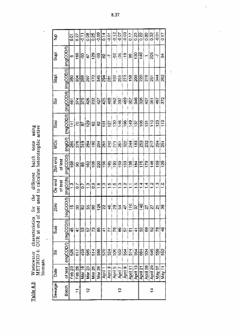
Tab
le 8
.3:
Was
tew
ater
ch
arac
teri
stic
s fo
r th
e di
ffer
ent
batc
h te
sts
usin
g M
ET
HO
D 4
: O
UR
at
end
of t
est
used
to
calc
ulat
e he
tero
trop
hic
acti
ve
biom
ass.
Se
wa
ge
D
ate
Sti
Sus
i Z
bh
i O
e e
nd
Z
bh
en
d
Mo
c
Sbs
i o
f te
st
of t
est
B
atc
h
of t
est
(m
g C
OD
/I)
(mgC
OD
/1)
(mg
CO
D/I
) (m
g0
/1/h
) (m
gCO
D/1
) (m
g0/1
) (m
gCO
D/1
) F
eb
23
5
26
45
1
5
1.3
1
58
28
5 11
1 11
F
eb
28
617
47
30
0.7
90
2
76
7
0
Ma
r 18
4
59
5
3
82
0.7
8
9
31
9
87
12
M
ar
23
58
5
57
55
1.
3 1
63
28
4 12
9 M
ar2
6
514
73
80
0
.9
10
6
18
0
62
M
ar
28
588
85
1
26
1.
8 22
0 29
4 8
2
Apr
il 1
570
41
22
1.3
1
56
26
1 13
1 A
pril
3 52
4 77
46
1
.5
18
5
242
127
Apr
il 5
506
78
29
1
.5
19
0
271
13
0
----·-·----·
13
A
pri
l 7
502
86
54
1
.3
159
261
14
6
Ap
ril
9 55
4 57
47
1
.2
15
3
322
19
6
Ap
ril
11
574
61
11
0
1 .1
1
38
24
4 1
49
A
pri
l 13
55
4 41
37
1
.5
18
4
18
3
137
Ap
ril
21
664
52
14
0
1.4
1
76
25
3 1
06
A
pril
28
504
69
27
1
.4
17
9
23
2
131
14
Apr
il 29
64
5 52
27
1
.2
14
8
217
11
0
Ma
yo
?
55
8
78
21
1.
3 1
59
29
4 1
23
M
ay
11
552
46
39
1.0
12
9
251
11
0
Sbi
S
bp
i
(mgC
OD
/1)
(mgC
OD
/1)
461
350
37
4.
304
375
288
426
297
232
17
0
427
345
42
5
29
4
408
281
462
33
2
-----
397
251
469
273
307
15
8
34
6
20
9
32
6
220
407
276
361
251
467
344
37
2
262
Su
pi
(mgC
OD
/1)
6 16
6
-50
47
1
29
-5
0 8
2
-7
-62
-35
-19
96
1
30
14
6"
1 2
05
-7
9
4
fup
0.01
0.
27
-0.1
1 0.
08
0.25
-0
.09
0.1
4
-0.0
1 -0
.12
-0
.07
-0.0
3 0.
17
0.23
0
.22
0
.00
0
.32
-0
.01
0.17
00
w
~

8.38
Table 8.4: Heterotroph active biomass yield coefficient for acetate added to the batch test.
Acetate Equivalent Amount of Heterotroph yield OUR area COD COD added (Yzh)
(mg0/1) (mgCOD/1) (mgCOD/1) (mgCOD/mgCOD) 33 99 102 0.676 38 114 102 0.627 36 108 102 0.647 39 117 102 0.618 31 93 102 0.696 39 117 102 0.618 37 111 102 0.637 34 102 102 0.667 37 111 102 0.637 38 114 102 0.627 35 105 102 0.657
Mean= 0.646 SDmean= 0.007

8.39
Table 8.5a: Wastewater characteristics for the batch tests using METHOD 5: Acetate addition at the end of the batch test.
Sewage Dates of Sti Sus Batch tests (mgCOD/1) (mgCOD/1)
14 May? 558 78 May27 534 41
15 May30 525 49 June 24 469 38 June 26 497 44 June 27 533 36
16 June 29 441 28 June 30 545 32 July 1 464 36
17 Julys 504 38
Sewage Dates of Zee Supi Batch tests (mgCOD/1) (mgCOD/1)
14 May? 37 156 May 27 39 165
15 May30 24 224 June 24 23 229 June 26 33 152 June 27 32 210
16 June 29 31 24 June 30 34 129 July 1 30 85
17 July 5 34 50 Ste= theoretical end of test COD CODend=measured end of test COD.
Zbhi Zbhe (mgCOD/1) (mgCOD/1)
21 38 39 36 33 57 11 21 27 44 44 45 29 113 34 95 64 99 49 123
fus fup
0.14 0.28 0.08 0.31 0.09 0.43 0.08 0.49 0.09 0.31 0.07 0.39 0.06 0.05 0.06 0.24 0.08 0.18 0.08 0.1
Oc Sbi (mg0/1) (mgCOD/1)
148 303 156 289 98 219 93 191
132 274 128 242 125 360 137 349 120 278 137 367
Ste CODend (mgCOD/1) (mgCOD/1)
410 286 377 332 427 263 376 329 365 313 405 337 316 282 408 282 343 294 367 359

8.40
Table 8.5b: COD recovery for acetate added to batch tests (see Table 8.5a).
Sewage Dates of Acetate Equivalent Amount of % COD OUR area COD COD added
Batch tests (mg0/1) (mgCOD/1) (mgCOD/1) recovery 14 7 May 35 104 102 102
27 May 37 110 102 108 15 30 May 29 87 102 86
24 June 25 75 102 74 26 June 34 102 102 100
16 27 June 35 105 102 103 29 June 33 98 102 96 30 June 31 94 102 92 1 July 39 117 102 115
17 5July 38 115 102 113 Mean= 99
SDmean= 4

8.41
Table 8.6: Wastewater characteristics for different batch tests using METHOD 6:
Sewage Batch
17
18
19
20
Flocculated-filtered raw sewage filtrate addition at the end of the batch test.
Dates of Sti Sus Zbhi Zbhe . Oc Sbi tests (mgCOD/1) (mgCOD/1) (mgCOD/1) (mgCOD/1) (mg0/1) (mgCOD/1) july 7 492 52 70 181 213 324 july 9 504 24 44 303 160 419
july 12 530 40 18 267 148 397 july 13 514 45 20 158 146 284 july 14 534 45 28 196 211 379 july 15 567 49 36 110 195 269 july 16 551 53 57 116 169 228 july 18 461 61 44 200 164 319 july 19 486 12 42 114 149 221 july 21 518 37 77 122 219 264 july 25 469 37 50 183 176 309 july 27 545 29 38 172 175 309 july 28 555 43 40 113 219 292 july 29 451 43 16 161 177 322 Aug 1 437 25 10 136 197 322 Aug 2 519 25 29 73 246 289 Aug 4 503 49 40 91 257 308 Aug 5 443 49 36 71 213 247 Aug 6 511 41 80 116 247 282 Aug 7 510 41 27 93 264 331
Aug 16 545 37 22 186 273 438 Aug 18 506 45 26 169 246 389 Aug 19 549 33 65 200 291 426 Aug 20 579 56 56 141 297 382 Aug 28 584 39 59 195 288 424 Aug 30 567 39 55 185 202 333 Sept 2 606 57 66 137 339 410 Sept 4 526 49 29 233 231 435 Sept 6 520 41 24 69 231 275 Sept 7 520 27 17 61 259 302 Sept 8 525 31 29 74 296 342 Sept 9 508 41 38 126 241 330
Sept 11 483 53 53 59 250 257 Sept 13r 525 45 40 55 197 213 Sept 131 525 45 54 104 187 237 Sept 15 411 41 69 87 245 263

8.42
Table 8.6 (cont.): Wastewater characteristics for different batch tests using
Sewage Batch
17
18
19
-20
METHOD 6: Flocculated-filtered raw sewage filtrate addition at the end of the batch test.
Dates of Zee Supi fus tests (mgCOD/1) (mgCOD/1) july 7 24 46 0.11 july 9 5 17 0.05
july 12 4 75 0.08 july 13 12 166 0.09 july 14 20 83 0.08 july 15 24 213 0.09 july 16 21 213 0.10 july 18 13 36 0.13 july 19 17 210 0.03 july 21 30 141 0.07 july 25 17 73 0.08 july 27 17 169 0.05 july 28 28 180 0.08 july 29 16 70 0.10 Aug 1 21 80 0.06 Aug 2 35 176 0.05 Aug 4 36 106 0.10 Aug 5 30 111 0.11 Aug 6 35 108 0.08 Aug 7 35 112 0.08
Aug 16 29 48 0.07 Aug 18 27 46 0.09 Aug 19 34 25 0.06 Aug 20 39 85 0.10 Aug 28 34 62 0.07 Aug 30 21 141 0.07 Sept 2 47 73 0.09 Sept4 20 13 0.09 Sept6 32 180 0.08 Sept 7 37 174 0.05 Sept 8 42 123 0.06 Sept 9 30 100 0.08
Sept 11 38 121 0.11 Sept 13r 29 228 0.09 Sept 131 25 190 0.09 Sept 15 36 38 0.10
Ste = Theoretical end of test COD. CODend= measured end of test COD.
fup Ste CODend (mgCOD/1) (mgCOD/1)
0.09 279 · 347 0.03 344 371 0.14 382 397 0.32 368 397 0.16 323 259 0.38 372 243 0.39 382 379 0.08 298 310 0.43 337 326 0.27 300 392 0.16 293 228 0.31 370 361 0.33 336 334 0.16 274 269 0.18 240 242 0.34 273 267 0.21 246 260 0.25 231 252 0.21 264 297 0.22 246 301 0.09 271 236 0.09 260 219 0.05 258 295 0.15 282 319 0.11 296 260 0.25 365 344 0.12 267 283 0.02 295 309 0.35 289 287 0.33 261 297 0.24 228 309 0.20 267 273 0.25 233 244 0.43 328 277 0.36 338 305 0.09 166 167

Tab
le 8
.7:
Was
tew
ater
cha
ract
eris
tics
for
dif
fere
nt b
atch
tes
ts u
sing
ME
TH
OD
6:
Se
wa
ge
B
atc
h
21
23
Raw
sew
age
filt
rate
add
itio
n at
the
end
of
the
batc
h te
st
afte
r 2
or
mor
e da
ys.
Oat
es o
f S
ti S
usi
Zb
hi
Zb
he
O
c S
bi
Ze
e
test
s m
gCO
D/1
m
gCO
D/1
m
gCO
D/1
m
gCO
D/1
m
g0/1
m
gCO
D/1
m
gCO
D/1
S
ep 1
6 (3
) 4
84
33
9
6
81
230
251
37
S
ep 1
9(2)
58
3 44
9
3
81
245
245
39
S
ep 2
1 (2
) 58
3 37
31
1
02
24
6 24
6 3
2
Sep
231
(3)
517
58
55
15
2
259
259
33
S
ep 2
3r(2
) 51
7 7
2
43
202
211
211
20
S
ep 2
7r(2
) 55
6 41
6
5
10
5
197
197
27
Sep
271
(3)
556
43
57
85
24
4 24
4 3
5
Sep
30r
(2)
523
49
65
9
0
213
213
31
Sep
301
(3)
523
26
49
73
23
0 23
0 3
3
25 O
ct(4
) 56
1 4
5
52
1
09
3
13
31
3 44
25
Oct
(3)
· 56
1 41
4
9
10
5
27
2
27
2
38
28
Oct
(4)
50
6
53
47
6
9
243
243
36
28
Oct
(3)
50
6
31
39
1
18
25
6 2
56
33
3
Nov
(2)
53
9
63
7
44
25
6 25
6 3
7
3 N
ov(3
) 5
39
3
7
22
6
7
268
26
8
38
3
Nov
(4)
53
9
41
25
46
3
12
3
12
46
Su
pi
fus
fup
m
gCO
D/1
1
04
0.
07
0.21
1
75
0
.08
0
.30
1
66
0.
06
0.2
8
16
0.
11
0.0
3
12
0.
14
0.0
2
18
6
0.07
0
.33
1
49
0.
08
0.2
7
141
0.0
9
0.2
7
161
0.05
0.
31
51
0.0
8
0.0
9
10
6
0.0
7
0.1
9
10
5
0.0
9
0.21
6
8
0.0
6
0.1
3
13
9
0.1
3
0.2
6
13
0
0.07
0
.24
9
3
0.0
8
0.1
7
(2,3
,4)i
nd
ica
tes
len
gth
of t
ime
(d)b
atc
h t
est
is r
un
pri
or
to f
ilte
red
wa
ste
wa
ter
ad
dit
io
Ste
= T
he
ore
tica
l e
nd
of t
est
CO
D.
Ste
m
gCO
D/1
25
4 33
8 33
7 25
8 3
06
35
9 31
2 31
0 29
4 24
8 2
89
2
63
25
0 2
82
27
1 2
26
CO
De
nd
= m
ea
sure
d e
nd
of
test
CO
D.
CO
Oe
nd
m
gCO
D/1
26
2 33
0 29
1 24
4 30
3 36
7 35
1 36
7 35
1 25
3 29
0 24
9 24
3 2
75
26
6 22
4
00
..i
:,..
w

8.44
Table 8.8: Mean unbiodegradable particulate COD fraction of influent COD (fup), number of tests and standard deviation ·or the mean for the different sewage batches (see Tables 8.6 and 8. 7).
Sewage Unbiodegradable Particulate COD as % of Total COD (fup)
Batch test mean no. of std.
Batch % tests dev. of mean 17 0.20 10 0.04 18 0.18 10 0.02 19 0.08 6 0.03 20 0.22 9 0.04 21 0.23 9 0.04 23 0.18 7 0.02

CHAPTER 9
EVALUATION OF BATCH TEST EXTENSION TO DETERMINE SLOWLY BIODEGRADABLE AND UNBIODEGRADABLE
PARTICULATE COD
9.1 INTRODUCTION
In Chapter 8 extensions to the batch test procedure have been proposed to quantify
influent wastewater slowly biodegradable COD and unbiodegradable particulate
COD. Initial indications are that the values derived from the batch test compare
reasonably well with those expected for the raw (unsettled) municipal wastewater
tested. In this Chapter values derived from the batch test procedure will be
evaluated, by comparing these to values obtained from conventional methods. The
only conventional method to determine unbiodegradable particulate COD ( and
concomitantly slowly biodegradable COD) is that of Ekama et al. (1986) and this
method is adopted here.
9.2 METHOD
As described in Chapter 4, batches of wastewater were collected from the Mitchell's
Plain Wastewater Treatment Plant and stored in stainless steel tanks at 4 • C; this
served as influent for testing for a period of about two weeks. (Experience has
shown that storing the wastewater for a period longer than about three weeks would
result in the characteristics of the wastewater changing). Daily, after thorough
mixing, wastewater samples were drawn from the storage tanks and diluted to the
desired COD concentration (±500 mgCOD/t) using tap water. Using the same
wastewater at the same COD concentration, the extended batch tests as proposed in
Chapter 8 and a laboratory-scale unit were run in parallel.
The laboratory-scale unit was a completely aerobic single reactor system at 12 .days
sludge age and 20° C temperature. Operational procedures as described in detail by
Ekama et al. (1986), Burke et al. (1986), Clayton et al. (1989) and others were
followed. The layout and operational data for the system are summarized in Fig
9.1; details are given in Appendix D. The following measurements were made on
the system:
a) The COD concentration (Standard Methods, 1985) of the feed and filtered and
unfiltered COD concentration of the effluent.

9.2
b) The influent and effluent TKN concentration (Standard Methods, 1985).
c) The effluent nitrate concentration (Technicon Auto Analyzer).
d) The reactor mixed liquor suspended solids (MLSS) and mixed liquor volatile
suspended solids (ML VSS) (Standard Methods, 1985).
e) The oxygen utilization rate (OUR) in the aerobic reactor was measured twice a
day and the two readings averaged.
Detailed experimental data for the laboratory-scale unit are listed in Tables D.la
and b, Appendix D. From Ekama et al. (1986), the daily results for a particular
wastewater batch were averaged (see Tables D.1 and D.2, Appendix D). From the
average, for each wastewater batch, COD and nitrogen mass balances were
calculated using the procedure set out by Ekama et al. (1986). Mass balance results
are listed in Table D.2, Appendix D. Mass balances falling in the range 90-110%
are considered acceptable. For the nitrogen mass balances, with the exception of
sewage batch No.21 the mass balances were acceptable; sewage batch No.21 was
rejected for further analysis. However, the COD mass balances all were too high
(average mass balance 119%). The high COD mass balances were unexpected;
usually for completely aerobic activated sludge systems acceptable COD mass
balances can be obtained without undue difficulty. A number of parallel completely
aerobic activated sludge systems operated in the UCT laboratory by undergraduate
research students gave very similar COD mass balances (Ubisi, 1994; Jadav, 1994;
Hercules, 1994). The COD mass balance contains four elements (Ekama et al.,
1986) - COD of influent and effluent, oxygen utilization rate (OUR) for
carbonaceous material consumption (i.e. measured OUR minus the OUR for
nitrification) and sludge production (i.e. mixed liquor volatile suspended solids
concentration measured as COD multiplied by the waste flow rate). The acceptable
nitrogen mass balances indicated the OUR for nitrification was reasonable.
Investigations showed that the COD measurement technique was accurate ( checked
with standard potassium hydrogen phthalate, Standard Methods, 1985); the COD
data could be accepted. Simulations of the system response with the UCTOLD
computer programme (Dold et al., 1991) indicated that the problem with the COD
mass balance was located in errors in measurement of the oxygen utilization rate
(OUR). Thus, the OUR parameter could not be used to determine the
unbiodegradable COD fraction (fup) (Ekama et al., 1986). Accepting that the error

9.3
in the COD mass balance was due to errors in OUR measurement, the measured
mixed liquor volatile suspended solids (MLVSS) parameter was accepted as
reasonable, and used to determine the fup (Ekama et al., 1986); using this method,
errors in the OUR measurement will not affect the estimate for fup· Accordingly,
from the averaged data the unbiodegradable soluble COD fraction (fus) was calculated as the effluent COD concentration divided by the influent COD
'
concentration. From the averaged data and calculated fus, the fup was calculated
using the following equation (Ekama et al., 1986):
where
MXv = total volatile solids mass (mgVSS)
=Xv·Vp
Xv = MLVSS concentration (mgVSS/t)
V p = system volume ( t)
=10 t Yh * = heterotroph active biomass yield (VSS units)
= 0,45 mgVSS/mgCOD
Rs = sludge age ( d)
= 12 d
bh * = net specific endogenous mass loss rate
= 0,24/d
f = endogenous residue fraction
=0,2
fcv = COD/VSS ratio of mixed liquor
= 1,48 mgCOD/mgVSS
MSti = total influent COD mass fed per day (mgCOD/d)
= Q·Sti
Q = influent flow rate
= 10 t/d
Sti =influent COD concentration (mgCOD/t)
(9.1)
For each batch of wastewater tested, successive values for fup were substituted into
Eq (9.1); the fup value that gave a theoretical MLVSS mass (MXv) equal to the
measured value was accepted. The fup values for the different wastewater batches

9.4
are listed in Table 9.1.
In parallel to the steady state unit, batch tests were run using the same wastewater
at the same COD concentration as fed to the steady state unit, and using the
extended procedure set out in Chapter 8, Section 8.8. Detailed data for the batch
tests are listed in Table 8.6. Data from the batch tests were anajyzed using the
procedures set out in Chapter 8, Section 8.8, and the fup values for each batch test
were determined. For each wastewater batch, the fup values from the different
batch tests were averaged, and are listed in Table 9.1.
9.3 COMPARATIVE ANALYSIS
For the different batches of wastewater tested, the average fup values for the
different wastewater batches from the conventional laboratory-scale system and the
batch tests are listed in Table 9.1; the fup values from the two methods are plotted
against each other in Fig 9.2.
Comparing the fup values derived from the two methods, the values for fup from the
batch test (fup = 0,08-0,22) and the conventional completely aerobic system (fup = 0,05-0,19) fall within the same range. Furthermore, the ranges of fup values from
both tests compare reasonably with those quoted in the literature for South African
raw municipal wastewaters (fup = 0,07-0,20; WRC, 1984). However, it is evident
that, with the exception of sewage batch No. 23, the direct correlation between the
fup values from the two tests for the individual batches of wastewater is poor. For
all the batches of wastewater tested, the fup values for the two methods were
averaged, see Table 9.1; on average the batch test gave fup values that tend to be
higher ( average fup = 0,17) than those from the conventional method ( average fup = 0,11). However, from Fig 9.2 no absolute discernible trend can be identified in the
relationship between the fup values from the two test methods. To identify clear
trends a more extensive experimental investigation is required, so that more data
are available. One aspect that will need to be investigated is the basic assumption
made in the batch test, that all the influent biodegradable (in particular slowly
biodegradable) COD has been consumed in the batch test prior to the addition of
the filtered raw wastewater. If this assumption is not correct, then the
unmetabolized influent slowly biodegradable COD will be reflected as
unbiodegradable particulate COD, leading to an overestimation of this COD
fraction, a general trend observed in the batch test. The degradation kinetics for
the slowly biodegradable COD will depend on a number of factors, inter alia, the

9.5
heterotroph active biomass concentration, acclimatization of this biomass to the
specific organic compounds making up the slowly biodegradable COD, and the
degradability of these specific organic compounds. To ensure in the batch test that
all the slowly biodegradable COD has been consumed, the batch test would have to
be run for a considerable period, which would make the batch test less attractive for
practical application. In any event, it was shown in Chapter 8 that increasing the
length of time of the batch test did not provide consistent results.
Since the unbiodegradable particulate COD tends to be overestimated in the batch
test compared to the continuous test (accepted as the datum), the slowly
biodegradable COD should be underestimated; the slowly biodegradable COD
(Sbpi) is found by subtracting all the other COD fractions from the total COD (Sti),
i.e.
(9.2a)
(9.2b)
where
fts = fraction of influent total COD which is readily biodegradable
= SbsJSti fus = fraction of influent total COD which is unbiodegradable soluble
= SusJSti fzbh = fraction of influent total COD which is heterotroph active biomass
= ZnHJSti
For the batch test method, all the information required to calculate Sbpi in Eq
(9.2b) can be determined from the test procedure, see Table 9.1. For the completely
aerobic activated sludge system, however, estimates for fts and fZbh cannot be
obtained from measurements made on this system - for the purposes of calculation,
fZbh from the batch test was used and fts from a parallel flow-through square wave
system (WRC, 1984), see Table 9.1. The slowly biodegradable COD as a fraction of
total COD (fbp) from the batch tests and conventional completely aerobic system
for the different wastewater batches are listed in Table 9.1. For the different
wastewater batches, in Fig 9.3 the average slowly biodegradable COD as a fraction
of total COD (fbp) from the batch test are plotted against those from the
conventional test; again the direct correlation between the values for fbp from the

9.6
two test methods is poor. For all the batches of wastewater tested, the fbp values
for the two methods were averaged, see Table 9.1; as expected, the average fbp
estimate from the batch test (average fbp = 0,44) is lower than that from the
completely aerobic system (average fbp = 0,51). Again, as for the fup values, from
Fig 9.3 no discernible trend can be identified in the relationship between the fbp
values from the two test methods. However, because the absolute v~lues for fbp are
very much larger than those for fup, the relative difference between fbp estimates
from the two tests are smaller than the relative difference between fup estimates.
9.4 CONCLUSIONS
Although the proposed extension to the batch test method to determine slowly
biodegradable (Sbpi) and unbiodegradable particulate (Supi) COD fractions in the
influent, provides estimates for Sbpi and Supi that fall in the same range as
estimates from the conventional completely aerobic activated sludge system method
(Ekama et al., 1986), the direct correlation between the estimates from the two
methods is poor. The batch test method provides estimates for Supi that tend to be
higher than those derived from the conventional activated sludge method, and
correspondingly provides estimates for Sbpi that tend to be lower than those derived
from the conventional activated sludge method. A more extensive experimental
evaluation is required to discern if these trends are consistent, but they would
suggest that the basic assumption for the batch test - that the slowly biodegradable
COD has been consumed prior to addition of the filtered raw wastewater - may not
be valid. This requires further investigation. For the present, the batch test does
not provide estimates for fup that are sufficiently accurate and precise for use in
design and simulation of activated sludge systems. For design and simulation, fup
should be able to be quantified into the ranges 0-0,05; 0,05-0,10; 0,10-0,15; etc.
As yet, there is not sufficient surety that the estimate for fup from the batch test
will meet this requirement.

Fig 9.1:
Influent
QI= 101/d
reactor
VP= 101
9.7
Waste Sludge Rs= 12d Secondary
settling tank
Effluent
Sludge recycle
1:1
Configuration of aerobic activated sludge unit used for the conventional method (Ekama et al., 1986) for determination of effluent COD and unbiodegradable particulate COD.

Fig 9.2:
Fig 9.3:
9.8
0.25~--------,----~-----------,,,
- • en Q) -..c 0.20~-------.-~---+-------:;,'--------j (J
iii cc 6
• • I
o 0.15-1-----------i------;!4----~----j (.) Ol E 0 0 (.) 0.10-1---------7"------+---------j Ol
.s a. :::J -
•
I o.o, /
0.00 . 0.00 0.05 0.10 0.15 0.20
Mean fup (mgCOD/mgCOD): Aerobic reactor 0.25
Comparison of the particulate unbiodegradable COD fractions (fup) from the batch test versus those from the completely aerobic activated sludge unit. Each data point represents the mean of a number of tests on one batch of sewage.
-en Q) -..c (J
iii cc
6 0 (.) Ol E ---0 0 (.) Ol
.s a.
.!) -C
0.70
0.60
0.50
0.40
0.30
0.20
CCI Q) ~ 0.10
• •
I I • • I
!·
0.00-t------r----r---r----r-----r---+----1 0.00 0.10 0.20 0.30 0.40 0.50 0.60
Mean fbp (mgCOD/mgCOD): Aerobic reactor 0.70
Comparison of particulate biodegradable COD fractions (fbp) from the batch test versus those from the completely aerobic activated sludge unit. Each data point represents an average of a number of tests on a batch of sewage.

Tab
le 9
.1:
SE
WA
GE
BA
TC
H
17
18
19
20
2
3
Ave
rage
Mea
n un
biod
egra
dabl
e so
lubl
e (f
us),
read
ily
biod
egra
dabl
e (f
ts),
un
biod
egra
dabl
e pa
rtic
ulat
e (f
up)
and
biod
egra
dabl
e pa
rtic
ulat
e (f
bp)
CO
D f
ract
ions
fro
m b
atch
tes
t an
d ae
robi
c un
it,
and
hete
rotr
oph
acti
ve
biom
ass
CO
D
frac
tion
(fz
nH*)
fr
om
batc
h te
st,
all
mgC
OD
/mg
tota
l in
flue
nt C
OD
. E
ach
valu
e re
pres
ents
a m
ean
of a
num
ber
of t
ests
on
a ba
tch
of s
ewag
e.
WA
ST
EW
AT
ER
CO
D F
RA
CT
ION
S (
mgC
OD
/mgC
OD
) A
erob
ic U
nit
Bat
ch T
est
mea
n rn
ean
mea
n m
ean
mea
n m
ea
n
mea
n fz
bh
* f:
ip
fus
fts
fbp
fu
p
fus
0.09
C
.09
0.08
0.
23
0.51
0.
20
0.08
0.
07
0.09
0.
08
0.26
0.
50
0.18
0.
08
0.08
0.
12
0.08
0.
24
0.48
0.
08
0.08
0.
07
0.05
0.
07
0.21
0.
60
0.22
0.
08
0.08
0.
19
0.08
0.
2 0.
45
0.18
0.
08
0.08
0.
11
0.08
0.
23
0.51
0.
17
0.08
m
ean
fzb
h*=
fro
m t
he b
atch
tes
t m
ean
fts f
or a
ero
bic
uni
t fro
m t
he
squ
are
wav
e te
st
mea
n fts
0.
27
0.25
0.
25
0.22
0.
18
0.24
mea
n fb
p
0.37
0.
42
0.51
0.
41
0.48
0.
44
co
co

CHAPTER 10
CONCLUSIONS AND RECOMMENDATIONS
10.1 OBJECTIVES
To comply with more stringent legislations controlling discharges of nutrients with
municipal effluents, over the past two decades there have been extensive
developments in the activated sludge method for wastewater treatment; the system
configuration and operation have increased considerably in complexity. With such
complexity, designs based on experience or semi-empirical methods no longer give
optimal performances; fundamentally based design procedures are required. Also, it
is not possible to make reliable quantitative or even qualitative predictions as to the
effluent quality to be expected from a design or to assess the effect of a modification
on a system without a kinetic model that simulates the system behaviour
accurately.
To meet these requirements, increasingly sophisticated design and simulation models
have been developed. As input to these models, it is necessary to characterize the
wastewater, that is, to quantify the various influent carbonaceous (C), nitrogenous
(N) and phosphorus (P) constituents making up the wastewater - the design or
simulation will be only as reliable as the wastewater characteristics that serve as
input.
The principal objective of this investigation was to evaluate and develop methods to
quantify the influent C material fractions (measured in terms of the COD
parameter). In reviewing the literature it was evident that existing methods to
quantify the C material fractions were either too elaborate or approximate; the
need exists for simple reliable methods for accurate estimation of these parameters.
To meet this requirement, a batch test method has been developed to quantify the
five influent COD fractions, namely heterotroph active biomass, readily
biodegradable COD (RBCOD), slowly biodegradable COD (SBCOD),
unbiodegradable particulate COD and unbiodegradable soluble COD. Also, the
physical flocculation-filtration method of Mamais et al. (1993) to quantify RBCOD
was evaluated and refined.
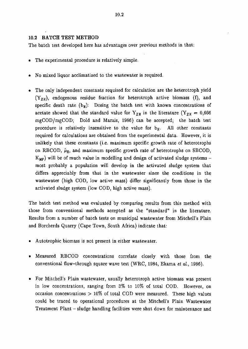
10.2
10.2 BATCH TEST METHOD
The batch test developed here has advantages over previous methods in that:
• The experimental procedure is relatively simple.
• No mixed liquor acclimatized to the wastewater is required.
• The only independent constants required for calculation are the heterotroph yield
(YzH), endogenous residue fraction for heterotroph active biomass (f), and
specific death rate (bH): Dosing the batch test with known concentrations of
acetate showed that the standard value for Y ZH in the literature (Y ZH = 0,666
mgCOD/mgCOD; Dold and Marais, 1986) can be accepted; the batch test
procedure is relatively insensitive to the value for bH· All other constants
required for calculations are obtained from the experimental data. However, it is
unlikely that these constants (i.e. maximum specific growth rate of heterotrophs
on RBCOD, µH, and maximum specific growth rate of heterotrophs on SBCOD,
KMP) will be of much value in modelling and design of activated sludge systems -
most probably a population will develop in the activated sludge system that
differs appreciably from that in the wastewater since the conditions in the
wastewater (high COD, low active mass) differ significantly from those in the
activated sludge system (low COD, high active mass).
The batch test method was evaluated by comparing results from this method with
those from conventional methods accepted as the "standard" in the literature.
Results from a number of batch tests on municipal wastewater from Mitchell's Plain
and Borcherds Quarry (Cape Town, South Africa) indicate that:
• Autotrophic biomass is not present in either wastewater.
• Measured RBCOD concentrations correlate closely with those from the
conventional flow-through square wave test (WRC, 1984, Ekama et al., 1986).
• For Mitchell's Plain wastewater, usually heterotroph active biomass was present
in low concentrations, ranging from 3% to 10% of total COD. However, on
occasion concentrations > 10% of total COD were measured. These high values
could be traced to operational procedures at the Mitchell's Plain Wastewater
Treatment Plant - sludge handling facilities were shut down for maintenance and

10.3
repairs and waste sludge recycled to the head of the works upstream of the point
where the wastewater was collected for the batch tests.
• For Borcherds Quarry wastewater, heterotroph active biomass concentration was
very variable, ranging from 7% to 16% of total COD. From an investigation of
operational procedures at the Borcherds Quarry Wastewater Treatment Plant, it
was found that intermittently waste activated sludge was recycled to the head of
the works and mixed with the incoming wastewater upstream of the point where
wastewater was drawn for the batch test.
• Although the values for wastewater heterotroph active biomass could not be
compared to conventional methods (none are available), the batch test was able
to detect correctly variations in heterotroph active biomass caused by changes in
plant operational procedures, as described above.
• Values for unbiodegradable soluble COD derived from the batch test compared
reasonably well with those derived from the effluent of a long sludge age
activated sludge system (Ekama et al., 1986).
• Values for unbiodegradable particulate COD derived from the batch test fall in
the same range as estimates from the conventional completely aerobic activated
sludge system method (Ekama et al., 1986). However, the direct correlation
between the values from the two tests is poor. For the present, the batch test
does not provide estimates for unbiodegradable particulate COD that are
sufficiently accurate and precise for use in design and simulation of activated
sludge systems. For design and simulation, unbiodegradable particulate COD as
a fraction of total COD (fup) should at least be able to be quantified into the
ranges 0-0,05; 0,05-0,10; 0,10-0,15; etc. As yet, there is not sufficient surety
that the estimate for fup from the batch test will meet this requirement; more
data are required.
• The errors in unbiodegradable particulate COD are reflected in the estimate from
the batch test for slowly biodegradable COD. However, because the absolute
value for the slowly biodegradable COD concentration is very much larger than
that for the unbiodegradable particulate COD concentration, the relative error in
the estimate for slowly biodegradable COD is very much less. The estimate for
slowly biodegradable COD can be accepted for design and simulation.

10.4
10.3 FLOCCULATION-FILTRATION METHOD
The :flocculation-filtration method proposed by Mamais et al. (1993) to determine
RBCOD was evaluated and refined also:
• The zinc sulphate :flocculannt recommended by Mamais et al. (1993) can be
replaced with aluminium sulphate. This has the advantage that pH adjustment
after :flocculation is not required.
• Measured RBCOD correlate reasonably with those from the conventional
flow-through square wave method (WRC, 1984; Ekama et al., 1986) and the
batch test method.
• The method is relatively simple and easy to apply, but requires independent
determination of unbiodegradable soluble COD, from effluent samples which may
not always be available.
• The 0,45µm filter papers recommended by Mamais et al. (1993) can be replaced
with glass fibre filter papers (Whatman's GF /C) to reduce costs, without any
loss in accuracy.
10.4 RECOMMENDATIONS
From this investigation, the following recommendations can be made:
• The batch test can be used successfully to determine the heterotroph active
biomass, RBCOD and the soluble unbiodegradable COD in the influent
wastewater. In this investigation, the estimates for RBCOD and
unbiodegradable soluble COD from the batch test could be compared to results
from conventional test methods. However, the heterotroph active biomass could
not be evaluated against any tests, because no such tests are available. To
evaluate estimates for heterotroph active biomass, it is recommended that an
inoculum of activated sludge mixed liquor from a defined continuous flow steady
state system is introduced into the batch test. From the steady state model
(WRC, 1984) the concentration of the heterotroph active biomass in the
continuous flow system and therefore added into the batch test can be calculated,
and compared to the concentration obtained from the batch test. However, due
account must be taken of nitrification, since the mixed liquor dosed to the batch
test may ni trify.

10.5
• For the batch test method, a technique has been developed to quantify the
unbiodegradable particulate COD and slowly biodegradable COD fractions.
However, direct correlation of estimates for these parameters from the batch test
and conventional tests were poor. Also, no discernible trends could be identified
in the relationship between values from the two tests. To identify clear trends, a
more extensive experimental investigation is required, so that more data are
available.
• This investigation has been restricted to quantifying the influent carbonaceous
material fractions. Similar studies need to be undertaken on the influent
nitrogenous and phosphoruos materials.

REFERENCES
Bhatla M N and Gaudy A J jr. (1965). Role of protozoa in the diphasic exertion of BOD. Journal of the Sanitar En ineerin Division. Proceedings of the American Society of Civil Engineers. 91 (SA3 , 63-87
Blackall L L (1994). Molecular identification of activated sludge foaming bacteria. Wat.Sci.Tech, 29(7), 35-42.
Black and Veatch (1979). Design procedure for complete mixing activated sludge process. Civil-Environmental Division, PO Box 8405, Kansas City, M0.64114.
Boero G J. Eckenfelder W W jr. and Bowers A R (1991). Soluble microbial product formation in biological systems. Wat.Sci.Tech, 23( 4-6), 1067-1076.
Bartone G, Chech J S, Germirli F, Bianchi R and Tilche A (1994). Experimental approaches for the characterization of a nitrification/denitrification process on industrial wastewater. Wat.Sci.Tech, 29(7), 129-136.
Bunch R L, Barth E F and Ettinger M G (1961). Organic materials in secondary effluents. J.Wat.Poll.Contr.Fed, 33(2), 122.
Burke R A, Dold P L and Marais GvR (1986). Biological excess phosphorus removal in short sludge age activated sludge systems. Res.Rept.W58, Dept. of Civil Eng, Univ. of Cape Town, Rondebosch 7700, South Africa.
Busch A W (1958). BOD progression in soluble substrates. Sewage and Industrial Wastes, J.Wat.Poll.Contr.Fed, 30, 1336.
Butterfield C T, Purdy W C and Theirault E J (1931). Studies on natural purification in polluted water - IV The influence of plankton on the biochemical oxidation of organic matter. Public Health Report, US Govt. Printing Office, Washington DC, 46, 393.
Chudoba J (1985). Quantitative estimation in COD units of refractory organic compounds produced by activated sludge microorganisms. Wat.Res, 19(1), 37-43.
Chudoba J, Cervenka J and Zima M (1969). Residual organic matter in activated sludge process effluents: IV - Treatment of municipal sewage. Technol.Water, 14, 5.
Clayton J A, Ekama G A, Wentzel M C and Marais GvR (1989). Denitrification kinetics in biological nitrogen and phosphorus removal activated sludge systems. Res. Rept. W63, Dept. of Civil Eng, Univ. of Cape Town, Rondebosch 7700, South Africa.
Daigger G T and Grady C P L (1977). A model for the bio--oxidation process based on product formation concepts. Wat.Res, 11, 1049.
De Walle F B and Chian E S K (1974). Removal of organic matter by activated carbon columns. Jour.Env.Eng.Div, ASCE, 100, SA3, 1089.
Dold P L, Ekama G A and Marais GvR (1980). A general model for the activated sludge process. Prag.Wat.Tech., 12(6), 47-77.

R.2
Dold P L, Bagg W K and Marais GvR (1986). Measurement of readily biodegradable COD fraction in municipal wastewater by ultrafiltration. UCT Report No. W57, Dept Civil Eng., Univ. of Cape Town, Rondebosch 7700, South Africa.
Dold P L and Marais GvR (1986). Evaluation of the general activated sludge model proposed by the IAWPRC task group. Wat.Sci.Tech, 18, Copenhagen, 63-89.
Dold P L, Wentzel M C, Billing A E, Ekama G A and Marais GvR (1991). Activated sludge simulation programs. Pub. by Water Research Commission, P O Box 824, Pretoria, 0001, South Africa.
Ekama G A and Marais GvR (1979). Dynamic behaviour of the activated sludge process. J.Wat.Poll.Contr.Fed., 51, 534-556.
Ekama G A, Dold P L and Marais GvR (1986). Procedures for determining influent COD fractions and the maximum specific growth rate of heterotrophs in activated sludge systems. Wat.Sci.Tech., 18, 91-114.
Gaudy A F (jr) and Gaudy E T (1980). Microbiology for Environmental Scientists and Engineers. McGraw-Hill Book Company.
Germirli F, Orhon D and Artan N (1991). Assessment of the initial inert soluble COD in industrial wastewaters. Wat.Sci.Tech, 23, 1077-1086.
Gloor R, Leidner H, Wuhrmann K and Fleischmann T (1981). Exclusion chromatography with carbon detection. A tool for further characterisation of dissolved organic carbon. Wat.Res, 15( 4), 457-462.
Government Gazette (1984). Regulation No. 991, Republic of South Africa Government Gazette No. 9225, 18 May 1984.
Grady C P L and Williams D R (1975). Effects of influent substrate concentration on the kinetics of natural microbial populations in continuous culture. Wat.Res, ~(2), 171-180.
Grady G P L jr, Kirsch E J, Koczwara K M, Trgoycich B and Watts R D (1984). Molecular weight distribution in activated sludge effluents. Wat.Res, 18(2), 239-246.
Gujer W, Henze M, Mino T, Matsuo T, Wentzel M C and Marais GvR (1995). The activated sludge model No.2: Biological phosphorus removal. Wat.Sci.Tech, 31(2), 1-12.
Henze M, Grady C P L (Jr), Gujer W, Marais GvR and Matsuo T (1987). Activated Sludge Model No.l. IA WPRC Scientific and Technical Report No.I, IA WPRC, London.
Henze M (1989). The influence of raw wastewater biomass on activated slud~e oxygen respiration rates and denitrification rates. Wat.Sci.Tech., 21(6/7), 603-609.
Henze M (1991). Nitrate versus oxygen utilization rates in wastewater and activated sludge systems. Wat.Sci.Tech, 18, 115-122.

R.3
Henze M (1992). Characterization of wastewater for modelling of activated sludge process. Wat.Sci.Tech, 25, 1-15.
Henze M, Gujer W, Mino T, Matsuo T, Wentzel M C and Marais GvR (1995). Activated sludge model No.2. Scientific and Technical Report No.3, IA WQ, London.
Hercules S M (1994). Characterization of C, N & P in wastewater. BSc (Eng) thesis, Dept. Civil Eng, Univ. of Cape Town, Rondebosch 7700, South Africa.
Hunter J V and Heukelekian H (1960). Separation and material balance of solids fractions in sewage. Proc. 15th Ind.Waste Conf, Purdue University.
Jadav M H (1994). Inorganic settleable solids accumulation in activated sludge reactors. BSc (Eng) thesis, Dept. Civil Eng, Univ. of Cape Town, Rondebosch 7700, South Africa.
Javornicky P and Prokesova U (1963). the influence of protozoa and bacteria upon the oxidation of organic substances in water. Int.Revue der Gesamten Hydrobiologie, 48, 335.
Kappelar J and Gujer W (1992). Estimation of kinetic parameters of heterotrophic biomass under aerobic conditions and characterization of wastewater for activated sludge modelling. Wat.Sci.Tech., 25(6), 125-140.
Leidner H A, Fleischmann T and Hamer G (1984). Molecular weight fractionation for the study of complex biodegradation processes. Analytica Chimica Acta, 163, 35-42.
Lesouef A, Payraudeau M, Rogalla F and Kleiber B (1992). Optimizing nitrogen removal reactor configurations by on-site calibration of the IA WPRC Activated Sludge Model. Wat.Sci.Tech., 25(6), 105-124.
Liebeskind M and Dohmann M (1994). Improved method for activated sludge biomass determination. Wat.Sci. Tech, 29(7), 7-14.
Mamais D, Jenkins D and Pitt P (1993). A rapid physical-ehemical method for the determination of readily biodegradable soluble COD in municipal wastewater. Wat.Res., 27(1), 195-197.
Marais GvR and Ekama G A (1976). The activated sludge process Part 1 - Steady state behaviour. Water SA, i( 4), 163-200.
McWhorter T Rand Heukelekian H (1962). Growth and endogenous phases in the oxidation of glucose. 1st Int.Con£. on Wat.Poll.Res, London.
Moosbrugger R E, Wentzel M C, Ekama G A and Marais GvR (1992). Simple titration procedures to determine H2C0 3*alkalinity and short-ehain fatty acids in aqueous solutions containing known concentrations of ammonium, phosphate and sulphide weak acid/bases. Water Research Commission, P 0 Box 824, Pretoria 0001, South Africa.
Moosbrugger R E, Wentzel M C, Ekama G A and Marais GvR (1993). A 5 pH point titration method for determining the carbonate and SCF A weak acid/bases in anaerobic systems. Wat.Sci.Tech, 28(2), 237-246.

R.4
Namkung E and Rittman B E (1986). Soluble microbial products (SMP) formation kinetics by biofilms. Wat.Res, 20(6), 795-806.
Nicholls H A, Pitman A R and Osborn D W (1985). The readily biodegradable fraction of sewage: its influence on phosphorus removal and measurement. Wat.Sci.Tech., 17, 73-87.
Pitman A R (1991). Design considerations for nutrient removal activated sludge plants. Wat.Sci.Tech, 23( 4/6), 781-790.
Randall E W, Wilkinson A and Ekama G A (1991). An instrument for the direct determination of oxygen utilization rate. Water SA, 17(1), 11-18.
Saunders F M and Dick R I (1981). Effect of mean-cell residence time on organic composition of activated sludge effluents. J.Wat.Poll.Contr.Fed, 53(2), 201-215.
Scientific Tables (1975). Edited by K Diem and C Lentner, CIBA-GEIGY, Basie, Switzerland.
Siebritz I P, Ekama G A and Marais GvR (1983). A parametric model for biological excess phosphorus removal. Wat.Sci.Tech, 15(3/4), 127-152.
Sollfrank U and Gujer W (1991). Characterization of domestic wastewater for mathematical modelling of the activated sludge process. Wat.Sci.Tech, 23( 4/6), 1057-1066.
Sutton P M, Jank B E, Monaghan B A and Murphy K L (1979). Single sludge nitrogen removal systems. Research Report No.88, Water Technology Centre, Burlington, Canada.
Standard Methods (1985). Standard methods for the examination of water and wastewater. 16th Ed. Pub. by American Public Health Assoc., 1015 Fifteenth Str. NW, Washington DC 20005, USA.
Still D, Blackbeard J R, Ekama G A and Marais GvR (1986). The effect of feeding patterns on sludge growth rate and sludge settleability. UCT Report No. W 55, Dept. Civil Eng., Univ. of Cape Town, Rondebosch 7700, South Africa.
Torrijos M, Cerro R M, Capdeville B, Zeghal S, Payraudeau M and Lesouef A (1994). Sequencing batch reactor: A tool for wastewater characterization for the IA WPRC model. Wat.Sci.Tech, 29(7), 81-90.
Ubisi M F (1994). Biodegradability of toilet paper. BSc (Eng) thesis, Dept. Civil Eng, Univ. of Cape Town, Rondebosch 7700, South Africa.
van Haandel A C, Ekama G A and Marais GvR (1981). The activated sludge process Part 3 - single sludge denitrification. Wat.Res, 15, 1135-1152.
van Haandel A C, Dold P L and Marais GvR (1982). Optimization of nitro$.en removal in the single sludge activated sludge process. Wat.Sci.Tech, 14(6/7), 443-461.
Velz C J (1950). Graphical approach to statistics. Water and sewaage works, Seranton Publishing Co, Chicago, Illinois 60601, USA.

R.5
Wentzel M C, Dold P L, Ekama G A and Marais GvR (1985). Kinetics of biological phosphorus release. Wat.Sci. Tech, 17(11/12), 57-71.
Wentzel M C, Dold P L, Loewenthal R E, Ekama G A and Marais GvR (1989a). Enhanced polyphosphate organism cultures in activated sludge systems. Part II: Experimental behaviour. Water SA, 15(2), 71-88. .
Wentzel M C, Dold P L, Ekama G A and Marais GvR (1989b). Enhanced polyphosphate organism cultures in activated sludge systems. Part III: Kinetic model. Water SA, 15(2), 89-102.
Wentzel M C, Ekama G A, Dold P L and Marais GvR (1990). Biological excess phosphorus removal - Steady state process design. Water SA, 16(1), 29-48.
Wentzel M C, Ekama G A and Marais GvR (1992). Processes and modelling of nitrification denitrification biological excess phosphorus removal systems - A review. Wat.Sci.Tech, 25(6), 59-82.
Wilson I S and Harrison M E (1960). The biochemical treatment of chemical wastes. J .Inst. of Sewage Purification, ,a, 261.
WRC (1984). Theory, Design and Operation of Nutrient Removal Activated Sludge Processes. Water Research Commission, P O Box 824, Pretoria 0001, South Africa.
Zehnpfennig R and Nichols MS (1953). Inoculation studies in BOD determination of sewage and pulp mill waste. Sewage and Industrial Wastes, J.Wat.Poll.Contr.Fed, 53, 61.

APPENDIX A
OUR-TIME PROFILES FOR THE BATCH TESTS.

FIG A.1 a OUR-time Plot for batch test 1 2 Ju1'9 3-Sewage Batch No.1
25-i---:.------,------IL'--------r---------r------,----.----------------. .Z. i ti;; 1420 mgCOD/1 * i te;;905 mgCOD/1
illEc* i . . ur oreo;;237 mg0/1 ttE* . . . / , * i i i BC0D;;254 mgCOD I 20 ....................................... t ....................................... : ........................................ ; ........................................ .; ........................................ j ....................................... .
A I I I ! ,,-....
L ..c -........_ 15 .......... 0 O> E
O:'. 1 0 ::J 0
* ! ! ! ! !
i~J_ J I J J i I 1 : ,
I *** I : **i : : **** . ;
r-···························r··············· "* • 1··.··. ···.····~----~····:·. * *····~···+··············· .................... .
r 0+------+------+------+-------+------+--------1
,,-.... L
_c
25
20
-........_ 15 .......... 0 O> E
O:'. 1 0 ::J 0
5
0
0 5
-.z. * ~
"' H* l!I
* * * *
* * ~
#-, -it =
l~~
10 15 Time (hrs)
20
FIG A. 1 b OUR-time Plot for batch test 1 9 Jul'9 3-Sewage Batch No. 1
/**** ** I(**** ~
~ 0 5 10
"'""' * l!I
* * * *
, 5
Time (hrs)
* ilE * *
70
25 30
Sti;;1311 mgCOD/1 STE;;1081 mgCOD /I RBC0D;;2 22 mgCOD /I OUR area;;245 mg0/1
* * *
25 30
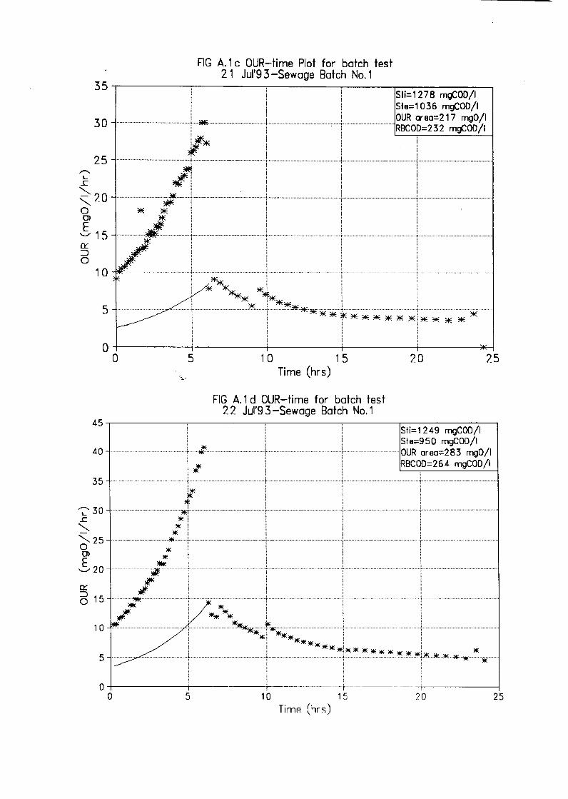
FIG A.1 c OUR-time Plot for batch test 2 1 Jul'9 3-Sewage Batch No. 1
35-,-~~~~~~~~~---,-~~~~---,-~~~-.-~~~~~---, , Sti=1278 mgCOD/1
, l . Ste=1036 mgCOD/1 1 1 J OUR areo=217 mg0/1 30 ............................................ r .... - .................................... l ........................................ , .... r ................................ RBCOD=232 mgCOD/1
~~ i i i 25 ···································:,j········· -- -!--- --···········i- -·················J····· - -------
::: 20 0 0)
51s
1 0
*
······················•········,:t········ .............. , ......................... j·.
5 ............................. .. ................. *. ...... i ..... ~.~*·** * .... ).. ....... ..... .... .. ....... + .............................. * ........ .. i *r******1**** ! !
O-+------+--------+------+-------t-------;,tE-1
0 5 1 0 1 5 20 25 Time (hrs)
FIG A.1 d OUR-time for batch test 2 2 Jul'9 3-Sewage Batch No. 1
45~-----------~----------,------.--------------, Sti=1249 mgCOD/1
40 1
Ste=950 mgCOD/1 • .. $: ............................... (................ . ...... ; .............................. OUR oreo=283 mg0/1
\ .;- j \ RBCOD=264 mgCOD/1
35 ... } l i 1 .••.•..••.••••••••••••••••••••••••••••••••••••••• "2 30 ............................................ *: ................................................ : .............................................. : .................. .
~ 25 ································~/··l················································l······················
S 20 .... ~~ ........ i .) ...................... .. ............ / .................... ! ................................................ ! ............................. .
~ ! **' !
Cl'.'.
~ 15
..................... ~* .... f**............... ; ········ .................................... _ ............................................ . *1 ***** : :
10
: *** : : ! *'* * * * * * * * *! * . r + ............................... t" .. "··-·,<· .... . 5
0 -l-------i--------~--- -+--· --15 0 5 10 20
Time (hrs) 25

FIG A. 1 e OUR-time for batch test 26 Jul'93-Sewage Batch No.1
30~------,--------,--------,--------~~~~~~ ...... i Sti=907 mgCOD/1
* l Ste=7 30 mgCOD/1 * I OUR area=160 mg0/1
25 ............................................... l... ............................. l1L* .... .l.. .................................. : .... : ................................. RBC0D=254 mgCOD/1
! • i i.1
:€ 20 ·····-··············-·····I···· -.--··-----1································· ···········1························· -i············ - -
~,s t •• • .. i I I I .............. ... I **** ! I I ~ i* i ! : :) ~ i . 0 1 0 ...................................... i .. T........... .. ................... T..... ............................... .. .......................................................................................... .
/. i .
s ;*-* I ... r • • • •. : ··· l ······~ ... • : :.·, * * *
! 0+-------+--------+--------+--------t---------, 0 5 10 15
Time (hrs)
FIG A. 1 f OUR-time for batch test 2 8 Jul'9 3-Sewage Batch No. 1
20 25
30~----------~--------,------,-~~~~~-:----, Sti=855 mgCOD/1
~ l Ste=439 mgCOD/1 * i OUR area=191 mg0/1
25 ................................. . ·······~1··~·······1······················· ·············r ··························RBC0D=257 mgCOD/1
r-,..
L 20 ..c:
""" """ 0 O> 15 E
~
:J 10 0
• ~ : J. .................................. ,,,_··············· ............................ .
···········································r·· ~---- ·· 1··························· ··;····
.;- i ............................. , ........................... !.................... + ·················t···· ····························-········
=7·1. · · .L. 1
......... 1:.············· 5 l4E: · · f ........ ~* *' ............................. .
*1**** * * *
0-+------+---------i-------+----------+--------j 0 5 10 15 20 25
Time (hrs)

FIG A.1 f OUR-time for batch test 2 8 Jul'9 3-Sewage Batch No. 1
30-.-~~~~~-.--~~-~---.-~-~~----.--~~~~-~---~ i I- Sti=855 mgCOD/1 l Ste=439 mgCOD/1 i * , . , OUR area=191 mg0/1
2 5 ............................................. r···················· .. ···:········ .. ···t .......................................... 't ......... RBC0D=2 5 7 mgCOD /I i * ! !
......... L 20 ..c
"-.. "-.. 0 O> 15 E
a::: :J 10 0
5
I • ! ! ! ! ** * : i •
: ** : : I ·············································-l-···········**····························l"························· .. ···············+··"····························"······ .. ···'1································"······· .. ···
I * I I I ! ! , ! ~ i i I
i *~* !
F i i *** i i i * * * ~ * * * * * :····:······:""":····; .. ··
:
1
0 -------------+i------+-------1'---------4 0 5 10 15
Time (hrs)
FIGA.2a OUR-time Plot for batch test 6 Aug'9 3-Sewage Batch No. 2
20 25
30~------,--------,-------.----,-------:--;----, ! Sti= 1214 mgCOD/1
* I Ste=960 mgCOD/1
~ :: ~~~ '.-- ~- -i--- j ~~o~:~~~g~~~: ~ *~ * I ! 15 ~-----------------------------------i------------------------------------------------1---------------------_ ••••••• -_.-_ •• -_.-_.--------- ------_-_._-_.-_.-_.-_-_-_-__ -._._.-__ -__ -____ ------·------·--·----·-·--·--------------------------------
0 10 *! 1
r** , : *** . *** i **iiE ; ,*** : ................................................. ;....... .. ... jli, .. * *' * iii: 'i,ji""iiii * * * 5
0 -+---------+--------+---·~ -
0 5 10
Time (hrs)
*!
1******* ..... .,..
- - -i--- -------'*"-1
20 25

Fig A.2b OUR-time Plot for batch test 9 Aug'93-Sewage Batch No.2
35.--------~------,--------,---------.----------------. ; Sti=1322 mg cod/I
# ! . Ste=1024 mgCOD/1 1 1 1 OUR area=2 1 0 mgO /I
i :: . :::~ : :1::: : :::::~::i:: : I : : ~:~=167.:gC:D:I , ,.;, * ! ! : : ~ 20
-l I I I ! .... - --E ., ; ; ; ; i 1 5 ............................................... , .................................... ·--· .. T........ .. I . ............. ............ .. -....... + ................................ -.. ..
0 ,o r~~==·,.~~===L··················· I ......... , / i i ***** i i 5 - .............................................. ) ............................................. )...... --~-~--f~ .. ~ . .* *·*·* .. llE·~f* *·*·-*·llLl!E .......... .
1
I . i
0 ---------<,--------+--,-----+--,------+-,--------< 0 5 10 15 20 25
Time (hrs)
FIG A.2c OUR-time Plot for batch test 13 Aug'93-Sewage Batch No.2
35~----------------,----------,-----..---------:-----, i Sti=1278 mgCOD/1
*i,
~ 30- ........................ ., .. ..
I* 25 ))Ii;
"2 *~ ~ * I "-. 20- ~ ......... 0 ,. 0)
E *
1 i I Ste=1113 mgCOD/1
\ . i : ~;~;JJ3~;,
i I I ······················· l ............. .; ....................................................... . ~ 15 _ JIL ................... . - ···-···········-··········-· ··················•·········· ..................... ··········································
O::'. :J 0
10
5 - ........ .
0 0
---··························- ····r···· ·················r······
i 0
l)lil!ile.,., : : ! ! ~111!191~ . ...,..i.w i ; ; ""*'01'M11181k;1e1~,1$1~ ~ , * t t r ~91~~*
I I , I I ·---·- -+--- -----~-------~, ------j
5 10 Vi 20 25 Time (hrs)
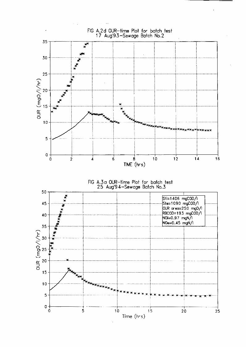
FIG A.2d OUR-time Plot for batch test 17 Aug'93-Sewage Batch No.2
35,--------,-------~---,---------,-!---------,-----~!----------,-----.,----,
* i !:. !,: l :,'
"JlW. i ! ! 3 0 .................. .. i i ~ ····················!.',,,,,,···· ························t·····························t······-·-···················· l ~~ l l I , ,
,. * ,. ,. · I I ! ! : 2 5 ............................. + ............................. i ............................. i ............................. ;. ........................... i .............................. i··········• .................. .; ............................ .
:* l : : i l i i4E ! ; i ! ! i
,.i I l I ...... 1 ............................... i.' ............................. 1 ............................. .
~·1 j --- -1- - -1 ~ -11 l : ···-* .. ·········· .. ···t···························-r--··· ··················t ·····;;·············· t··········· .......... ···j···· ................ \···· --1···• ........................ .
~ 10 •................. ·········:·· -~ .......... 1 ...................... 1 ......................... j .......................... . i ~***""*'" : i ; ! """'**************** ' j ! ..... /
0 +----+---------,----+------+------;------j------t-----t 0 2 4 6 8 10
TIME (hrs)
FIG A.3a OUR-time Plot for batch test 25 Aug'94-Sewage Batch No.3
12 14 16
50-.------------,--------,-. --------,-----------,-.--------,
! : I ! Sfi:;;1406 ~gCOD/1 45 ................. ~ ........................ + ............................................. + ............................................. +-········ ....... Ste=1090 mgCOD/1
* i i i OUR area=250 mg0/1 40 ............ ; .............................. i... ............................................. l... ........................................... .i ................ RBC0D=193 mgCOD/1
* 1 1 l NQi:;;0.97 mgN/1 * i i i NOe=0.45 mgN/1
35 ...... l····· ............................ t ................................................ i ............................................... i................. i
i : l i I I i:: : :i - r l 1 O'.'. 20 :::)
························*···················-1 ................................................ i .............. --·-················ ......... J ................................................ l ............................................... .
i--*··;~::1- I I i r******* : i
.. ·j· .... -t· * ¥ * * * * * * ~+* ,ti!·*···*---*···*····
0 15
10
5 ...................... .
0 +----------+------------------- --~r---------------------, 0 5 10 15 20 25
Time (hrs)

35
30
25 ,,-...
L ..c
'20
' 0 0)
S 15 Ct'.: ::J 0
,,-... L
..c
10
5
0
35
30
25
' ,20 0 0)
E ...._,, 15 Ct'.: ::J 0
10
5
0
* ** l~ *
* **
l~ *
-------
FIG 1 .3b OUR -time Plot for batch test 2 8 Aug'9 3-Sewage Batch No. 3
I I
"* Sti=126 7 mgCOD/1
* S1e=1028 mgCOD/1 * OUR area=188 mg0/1
** RBC0D=179 mgCOD/1 NOi=0.00 mgN/1
** * NOe=0.00 mgN/1
* * * .,
"'
A** ~ * ****** **--.,.........- '" ,._, ~* * ** ~ ll *
0 2 4 6 8
* * * *
"" -I *
""' * * *
"" * lE
-
*
3 5
Time (hrs) 7
FIG A.3c OUR-time Plot for batch test 29 Aug'93-Sewage Batch No.3
I
Sti=1205 mgCOD/1 S1e=962 mgCOD/1 OUR area=282 mg0/1 RBC0D=192 mgCOD/1 NOi=0.98 mgN/1 NOe=1.53 mgN/1
-
>--
9
I""-,: * w~
V ~*l4 *** IE"""
** *** ********* ~*****
---- -0 5 1 0 15 20 25
Time (hrs)

40
35
30
-L
..r: 25
' ' 0 O> 20 E ..........
O'.'. 15 :J
0
10
5
0
ME
* * ""'~
* * .....
l • ~
i #
I * J
FIG A.3d OUR-time Plot for batch test 31 AUGUST'93-Sewage Batch No.3
I
Sti=1071 mgCOD/1 S1e=763 mgCOD/1 OUR orea=281 mg0/1 ._ RBC0D=194 mgCOD/1 NOi=2.21 mgN/1 NOe=2.90 mgN/1
-
I *" .., "'· -,,#- /.
/ /
0 5
·--""~ *~
"'****i ~** *** ***** ~********)! ****
10 15 Time (hrs)
FIG A.3e OUR-time Plot for batch tes 1 Sept'93-Sewage Batch No.3
20
"' *"' * ***
25
45,-------il!E--------~----------~-----~ !
* ! Sti=1071 mgCOD/1 40 ................................................................................................ .L .............................................................. S1e=B52 mgCOD/1
( OUR area=312 mg0/1 i RBC0D=177 mgCOD/1
35 ·································~························································t······························································· NOi=0.96 mgN/1 * i NOe=0.96 mgN/1
...--..30 L
..r:
' ,25 0 0)
£20
............................... * ............................................................... ! ................................................................................................. , ............................................. .
................... / ........................................................... ~ ........................................................................................ j ............................................. . * ! j
···········!···········································································J·························································································l··············································
3:: ~-~ .... ~J............. Lz
i **** ****, i *************** :
...... 1...... ····························· ................ .l ··············································
I I 0 -------r---------+------- -T --+--------I
5
0 10 20 Time (hrs)

FIG A.3f OUR-time Plot for batch test 2 Sept'9 3-Sewage Batch No.3
35~---------~--,---------r----------, I Sti=1318 mgCOD/1
lWIE I Ste= 1079 mgCOD/1 30 - ·······························;·······························································r··············································:············ OUR area= 234 mg0/1
.,.. I RB~0D=169 mgCOD/1 25-····················-,······································································t···························································· N01=0.73 mgN/1
~ T i NOe=0.69 mgN/1 £ I l ~ lit': t' I "-.. 20 - ·············lie···················································· ........................... ................................................................................................. 1 ............................................... . 0 ~ i I rn *" I i E
/..* l !
I ! ~ 15 ............................................................................................. i·································································································;················································
6 10-7~w;;;;:~==:l:~~ ........ ~~ .... ~~ .. :::~~i~~"'***•;;: . 5 .................................................................................................. i ............................................................................................. i .............................................. .
I ! 0 4---------,-------i--,----~,------,i------~ 0 10 20
Time (hrs)
FIG A.4a OUR-time Plot for batch test 1 0 Sept'93-Sewage Batch No. 4
30.-------------,-----------.-------~ I Sti=497 mgCOD/1 [ Ste=362 mgCOD/1 J OUR oreo=114 mg0/1
2 5 ······························································································~··················································································· RBCOD=9 2 mgCOD /I llf ! NOi=0.06 mgN/1 * i NOe=0.00 mgN/1
Ct'. I i
6 , : ::~;~~ :~ ·--- _j~--------·----------·-----------------------------·-----------------1______ ---·---·- ---------·-* I *******************~*****
i J
0 +------~------+-------,-------;--------,o!E------j 0 1 0 20
Time (hrs)

FIG A.4b OUR-time Plot for batch test 11 Sept'9 3-Sewage Batch No.4
35~------------,.-,----------.-~~~~~/~-, 1 Sti=489 mgCOD I 1 Ste= 342 mgCOD/1
J l · OUR area=138 mg0/1 3 0 ......................................................................................... i~r·· ................................................................................ RBCOD= 1 0 4 mgCOD /I
* I * j •
25 .................................................................................... ! ........ 1 ................................................................................................. 1, ............................................... ..
~ * I I .C llE ; I
'-..... * 1 I ' 2 0 ............................................................................... ;-............. + ................................................................................................ 1 ............................................... .
i i I I '--"15 * ' ' § .............................................. * * : ······················· i
10 ................... = ................................... , ................................................................................... :.; ............................................ .. i
.......................................... ~ .......................... ~ ................................................................................. i ................ *,to!~ .. . i **** ~**** l **************, : : i ! i - 1 0;-------.---------------.------t-------l!E-!
0 10
Time (hrs)
FIG A.4c OUR-time Plot for batch test 12 Sept'93-Sewage Batch No. 4
20
14-.------i~------...,..-------,---r---------~ l* Sti=476 mgCOD/1
12
10 _...
L .c
' ' 8 0 CJ)
E * *
* *
j4E * Ste= 293 mgCOD/1 ti * ! j OUR area= 120 mg0/1 NOi &NOe=0.00 mgN/1 RBC0D=83 mgCOD/1
,.,,;l's ! \ :.= ! '--" 6 "')li( . . . ....................................... .. ................................... ..
Ck:'. * i i i '=,:.
6 I I I i !
4 .............................................. i .......... ~~ .................................... :.. .............................................. L ... ~~*-~-....... .. ! ! ***** ! **~* i i ****~********* !
I I 1 I .j............................ . .. '(-........ . ...... ······!·· ······································ ..... j. ...•••
I i i
0 -+---------+--------+--------------- -i--- --------·----t---------1
0 5 10 15 20 25 Time (hrs)
FIG A.4d OUR-time Plot for Batch test 9 Sept'9 3 r-Sewage Batch No. 4
18--,-------------,.-i-----------..--------, * I ti= 475 mgCOD/1
16 ·····································n················································I····································································· ~~=!::0=~~~0~~011
~ I Oi & NOa= 0.00 mgN/1 1 4 ······························································································+···································································· BCOD=B 7 mgCOD /I
~ 12 ..c
' '-.... 10 0 CJ)
5 8 O'.: ::J 0 6
4
* i * i ! - i i
' l ! i • l • l • l ............................................................................................... ; ...............................................................................................•............................................... * i i
: l l .................. l!L ..................................................................... ) .............................................................................................. ! .............................................. .
* i i
~ * ~i ~-- I ~ ~ ............ !
*'# ** j '**j * : ~
.................. ;....... ······································ ...................... ) ..... ~**~········--··*··········
! ! *** * 2 ........................................................................................... 1.............. . .................................................................... i. ·························
i i ! : l ! j ! o------~------+-----~--------------l
0 10 Time (hrs)
FIG A.4e OUR-time Plot for batch test 9 Sept'9 3L-Sewage Batch No.5
20
25~------: ••••.• i------*-------~-----.-~-!-~=-~-~-;-r;;,_g_g~-~-Dci_)_I ___,
"' OUR orao=163 mg0/1 RBCOD=B 9 mgCOD /I
-L ..c
20 ........... .
~ 15 "-.. 0 CJ)
E n'.: 1 0 ::J 0
,i. 1- i ··+-·············································
: * : i !········:·,,,
i i i
L1 * _J.......................... 1 ....................................... j * . i : :
; ! ! I ; j j
./ i \ r r···································· /1' !* * ~ ! !
5 .,.* .............................. ! ~~-~········· r*--r'~"-.;;;;;;;;;;··· 1 : l
i I 0 -+-------;----------+----~ .. + --~- --------i---------j
0 5 10 15 20 25 Time (hrs)

FIG A.4. f OUR-time Plot for batch test 1 3 Sept'9 3-Sewage Batch No.4.
35~------,--------r-----------,r------.------------:---, I Sti==436 mgCOD/1 · Ste=269 mgCOD/1
. ! ~ l OUR area=125 mg0/1 3 0 .............................................. '!" ............................................. :" ...... * ................................. l .............................. RBCOD== 1 0 3 mgCOD /I
; I * ;
~ 25 -- -- --1--- -- ---- --v-- -1- -+- -1: i i~ i I
j:: ~ t1 - -1 I 6
10 ~/J,, ..................... 1 J ! ~- l i
5 .... ~ ................. .!... . ....... ! .......... ~**"""············· ........................................... ! .......................................... . * i *** i i **** i * * *\ * * * * * * * * * i* * * * *
I I I 0-+-------+------+---------------<-----~
20
18
16
14 ,,-...,
L
..c 12
"' "' O 10 O> E
Cl:'.: 8 ::::)
0 6
4
2
0 5 10 15 Time (hrs)
FIG A.5a OUR-time Plot for batch test 2 1 Sept'9 3-Sewage Batch No. 5
;
f --1 T ·;···-r--··································-t-······························r
! I l ············•·········
20
Sti=5 71 mgCOD/1 Ste=356 mgCOD/1
25
·· OUR area= 1 6 9 mgO /I RBCOD== 1 2 3 mgCOD /I
...... ··-·•··-r· ·········-···················
*' t· t I -------------------- ------------r
.... ·····.lf··· ················· .................. ).......... .. ................. .
* * * ·····*··· *
· , ······· ·· ·········· · ·1·· ·-····················r . ................ T
i ~-::~: ...... •••• i•••••••·····················••••·····•••·• L~-~····.·. ! ****lli**********;
0 -+--------t-------+--~- - -- .. , 15 0 5 10 25
Time (hrs)

FIG A.Sb OUR-time Plot for batch test 19 Sept'9 3-Sewage Batch No.5
35-.----------,--------,--------,----.-St-i=~S~S-1-m-g~COO~/~I----,
Ste=376 mgCOD/1 , , , OUR area=161 mg0/1
3 o ············································r··············· ·························r····················· ...... ·:· ·····I······················-········ R8COQ; 1 o 4 mgCOD /I
25 ················································l··--··········································+··············································-1--·············································i·············································
'2- i I i ~
~ 20 ................................................ i ................................................ ! .............................................. ..1. ................................... /l ............................................. . % ~· I I i i
i :: ::~~~~-····1· ...................... r•·•· ··•• .. ·'···· .. ··.1···························••••••••·········
sL ....... • ... ~••••L,······················~. : i *
0-t------i-------+------+------~----_J 0 5 10 15 20 25
Time (hrs)
FIG A.Sc OUR-time Plot for batch tes 2 3 SEPT'9 3-Sewage Batch No.5
21 -.---------------,---------,-----,------------:----, Jj l Sti=551 mgCOD/1 ~*! i Ste=314 mgCOD/1
/ l i OUR ares=169 mg0/1
~ :: •.•••••................ / ...... 1............. . ................... 1 ............ ·· .... ·.··············· :························· .... R8CQD;12·~·~:00~I
l: .;- ~ i
~ 12 ......................................................... . '-... 0 O> E
'-../ 9 ..... l° ........................................... .
6 .... ,.. ·············+····· ······-··································
i i ***)!$IE***********~********** : \ i i
···-········--······ ·········-· -····t ·-········-··············· ················--i······ ........................... ·············~-
0 -+------+------+.----- . ' ------- .. ---j-------~ 0 5 10 15 20 25
Time (hrs)

FIG A.5d OUR-time Plot for batch test 16 Sept'93-Batch No.5
40-.-------,-------,.--------,-------,~~~~~~~--, ~d Sti= 546 mg COD/I
. ~ \ Sle=428 mgCOD/1
3 5 - .......................................... , ................................... * ..... ! ............ . .... ~~~o~:~~ ~ 7 ~g~6g ;11
* j
~ 30··· ~*~ r ;' ~ 2 5 - ............... :....... ...... i ...... ; .............. I. ................ .......... .. .· .. .. 0 *E i * l "'--.. * l i rn 2 0 - ..... >,. .......................... ........ ( .......................... llE ............... ).............. . .................................................... - .......................................... .
E * , ,
i 15 .;. * ........ : ................. ·························i······································ ·····1··············· ························
10 - ............................... iiii ...... ,t .............................................. ;. ............................................... ;................ ... . ............... '[ .......................................... .
5 ................................ ]~~~·~·*················L .................. i ......................•.................... 6-,-. : j ********~***** *****, ! ; . * ;
0 -+--------i--,------,~------i-, ------+--,--------1 0 5 10 15 20 25
Time (hrs)

FIG A.6 a OUR-timePlot for batch test 27 Sept'93-Sewage Batch No.6
35......-~~~~----,,--~~~~-,-~~~~~-,--~~~-,-~---~~-::-.:-:~--, j * i Sti= 638 mg COD/I
,,,....... L .c
30
, !3' ! Ste=395 mgCOD/1 \ illE . j OUR area=158 mg0/1
25
'20 ~ # * i * 1 ; ; i 15 / I ···· .. . ! Joc,tat, OO~tioo ! [ j
10 ........................... ·············+··································· · y--··· .................. · ......... + ··-t-·· .. . ......... · ......... . **! l iii, i
: ** l * i ** I .
··························-r--···················*·· ············--r-·····~~~:·············· ·r··· ········ ······· ··· ··1 ·············· **
i i ****~************** I I I 0-+-------+-------+-------+-------+-------j
0 5 10 15 Time (hrs)
FIG A.6 b OUR-time Plot for batch test 28 Sept'9 3-Sewage Batch No.6
20 25
35~------,-----------------,-------------~ * Sti=533 mgCOD/1
, Ste=386 mgCOD/1 ! , OUR area=143 mg0/1
30 ················································i···············································;································ ········r····························RBCOD=122 mgCOD/1
25 ; ) ................................................ ! ;* ; ································ ······························ '"2 ~ : ! *if* .c ~20
' 0 O')
S 15
~ * i I * 0
1 o ................................... * ... L. ......................................... L ......................................... ; .............. . ! !
·········*··········· /· . ·····························
* ; i *** ** ; * * *** *'** * ***"'" *: * 0 -l---------i------~~-f-~-- · t ---r -~------4
0 5 10 1 '.i 20 25 Time (hours)
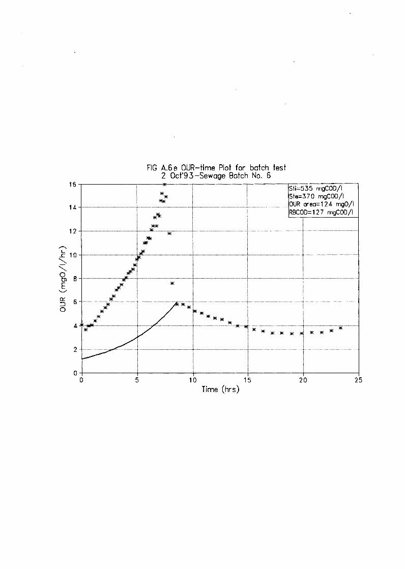
FIG A.6 e OUR-time Plot for batch test 2 Oct'9 3-Sewage Batch No. 6
16~-------------'~--~----------,------r---------:---,
~t L .. r·· ..... il!~~~~g:: 14 - ------------------ ---------
: ** 12 ---------------- -------------------------'---------*----------j( ________ ---· ......... ,-- ---··········-······················
! ~ i~
I······ ······················· ········ ...... 1 ·····································
'-Jf. i i l * ! #'' i
--·---·--------------il'-------t.... -------·---········-----t...---·-·······--··-·····-··-Jf< l * l
'tr } i
~ 6 .. ,,,, ___ ,,,,,,,_, __ *~-----------------! ....... __ ,,,, ...... ________ ,, .. ·-·*------!------·---------:] * i *= 0 * i ~ * ':, * i i * * l l * * * i i
4 *'M'I',---------------------·--------------+---------· -----........ _ ............ _,, ____ +----·--------·-----·--·--·-------*·---~--*-·------·------·--·----·------·-···+·-------------------------*---·-·-----! i i ****~***
I l l ······································································:············ ···r···· ................................ .
0+-------------------------------
2
0 5 10 15 20 25 Time (hrs)

FIG A. 7 a OUR-time Plot for batch test 5 Oct'9 3-Sewage Batch No. 7 ( diluted)
25--r-------,-----,-------,-----,-------,--,.---------------, l Sti=627 mgCOD/1
,,-._ L
..c
20
'-... 15 '-... 0 0)
E '-../
CY 10 ::J 0
* J *
1 . . . i Ste=471 mgCOD/1 j 1 1 1 \ OUR area=112 mg0/1 ! ~ ) ) J J RBC0D=100 mgCOD/1
* i l j ........... , ................ .... ~ .. -r .......................... j .......... . ........... ..\. . ....... j ........................... ..
r***** 1 . . **!)I,( i i ** *** *:*
T j ········ T ""*,.*f~ *" * :1~ : ~= I .
0-;------;------+-----t-----+-----+-----+-----l
0 2 4 6 8 10 12 14 Time (hours)
FIG A.7b OUR-time Plot for batch test 5 Oct'93-Sewage Batch No.7(undiluted)
50-r----~-----,-------,-----,------,---,---------------, Sti=1053 mgCOD/1
. , i 40 ............................... + ....... ~'* ... * ..... l ................................. r .............................. i ............................ r
i )ls j i
~ Jf* ! !
Ste=922 mgCOD/1 OUR area=210 mg0/1 RBCOD= 1 8 2 mgCOD /I
r l ~ 30 ........... * .. ; .... + ............................... ! ............................... , ......... .
'-... JIE . j i
.... r .... ....... 1 .................. T ....................... . 0 ~* ! l 0)
E '-../ g§ 20 ............................. T. 0
·············-···· ·····················-··· *'
......................... ···!················· ..... ········f-········ .......... -r····
0 -+-----t------t-------+----t------t-------+-------1
0 2 4 6 8 1 0 12 14
Time (hr)

FIG A. 7 c OUR-time Plot for batch test 6 Oct'93-Sewage Batch No.7(diluted)
20~-----.,---------,------~,----rS~ti=~6~2~7:--m~gC~O~D~/'I -----i
Er; !,,·:,::· Ste=471 mgCOD/1 OUR area=146 mg0/1
RBC0D=99 mgCOD/1 :
* i 15
* ···········································
5 ··········... .. .. . . ... . .................... ····· .... -~ -- ............. .
; **** ; ; **** : : *********** \ 1
0-+-------1f-------+-------+-------,t-------1 0 5 10 15 20 25
Time (hrs)
FIG A. 7 d OUR-time Plot for batch test 6 Oct'9 3-Sewage Batch No. 7 d (undiluted)
40,------,-----------,------,-----r-----~~--, j S1i=1106 mgCOD/1
················li·························· --·····!········ ............................ ···1. .. ~~l£r!;i:: l i
35
/
j j
30 .......................... J ....... i .............................................. l·········•............................. .................... ········1·· ......................................... ..
: : i ,.....__
J: 25
" " ~20 E
~ 15 0
10
5
........................ ~ ................. ; .......................................... ; ............................... .
*If * ~ * ; ; ............................... i ............................................... i ..................... .
: :
.............. J······ ._,.,""""'·
···················;········
... ·····-···········t··· ...... ~ ...
0 ;----------jr-------r--~----j-0 5 10 , 5
Time (hrs)
*
20 25

FIG A. 7 e OUR-time Plot for batch test 7 Oct'9 3-Sewage Batch No. 7 ( diluted)
40......-------------,-------------,-~~~~~~--, i Sti=607 mgCOD/1 j * Ste=446 mgCOD/1
35 ............................................................................................... ) .................................................................................. OUR area=161 mg0/1 i * RBC0D=91 mgCOD/1 i * i
30 ·································································································!·•··if ............................................................................... 1 ............................................... .
g§ 15 0
I* ! ! l
··································································································'r············································--················································---:---·············································
i ~ l *I * I ····························································································*·;·································································································;················································
i : * i
"' 4: * acetate addition
····································7~··········································1······················································································
10 ...... * ............................................... ·-*··· --r-·· ............................... .
5 ·············································· ·r···· ........ ~.!"".,r .. ,., .... ,, •• ,;,"r········ 0-+--------,r--------+------......--------ie----------1
0 10 Time (hrs)
FIG A. 7 f OUR-time Plot for batch test 8 Oct'9 4-Sewage Batch No. 7
20
18.....------,--------,------~----,---~~~----::----, \':: Sti=605 mgCOD/1
16 ................ .
14
,,......._
£ 12
" " i 10 E
6 .................. .
4
~ Ste=387 mgCOD/1
Z -I·· ·· ····· ··········· ··· ·· ··· i,.······ ····· ·· ~~~o~:;:1!!c~6;(1
*,:
#.. ,.. . ......•. I•·······.····································.···· .. •i•································•••••·•••••••••····
·······--·········-
.............................. ··································.
: ! ~~******* ** *~ ; : )I( '*****
.... *·· .
2--+--------i--------r----------r------r---------j 0 5 10 15 20 25
Time (hrs)

FIG A. 7 g OUR-time Plot for batch test 9 Oct'9 3-Sewage Batch No. 7
25~------,-------.,----------.-----.--~~---~-, ti=542 mgCOD/1
1. 1,,,,::. te=328 mgCOD/11 UR area=17 4 mgCOD/1
20 ······························;_··-(· - - --!·························· ····· 1·················· ......... Bt:~Drto~_i,'!J(:_~(1_
~ I I 1,,,,, ! ,,-.... L
~ 15 '-.._ 0 0)
E O". 1 0 ::J 0
~ , , I ........... j: ........................ i .............................................. l.................... .. : .......................................................................................... .
*•· 1 1 I 1. j j
l I : : .. * ... + ................................. ,+ .. .. . :.· ...................... t·
l
5 ........ ·········t········· -·r- .......... ~****~.. . .................... . ,****"" : "'***
o-------+-------------------------0 5 10 15
Time (hours)
FIG A.8a OUR-time Plot for batch test 22 Oct'93-Sewage Batch No.B(diluted)
20 25
24--r-------,-------..,.....----------,-----,---------. Sti=515 mgCOD/1
21
18
,,-....
l: 15 '-.._ '-.._
i 12 E
O". 9 ::J 0
6
3
... ;: ................. ! ............................................. ,,i',, ................................... .
~~ + -* --··················· ..................... ·······················
· ...................... t ......................... ~ .. * .. ~·~ .. 1 .. ;........ ...... .. · ·i
S1e=384 mgCOD/1 ......... OUR area= 1 6 8 mgO /I
RBC0D=63 mgCOD/1
i i * * * i : i * * *\ * * * * * *
.... ························· ..... -~ . - ... ··f ··· .. . . ··f ....
0 +-------+-------~--,·- - t
15 -f- --------1
0 5 10 20 25 Time (hrs)

24
21
1B
,-...
FIG A.Ba OUR-time Plot for batch test 22 Oct'93-Sewage Batch No.8(diluted)
Sti=515 mgCOD/1 * j , , Ste=3B4 mgCOD/1
--------------------------------~------------(---------------------------------------------)-------------------------------------------------l----------------------------------- OUR oreo=168 mg0/1 r ! 1 i RBC0D=6 3 mgCOD /I
~ 15 ......._ ......._
i12 E
'-/
O:'.'. :)
0 9
6
3
-------------------------------~---------t- ________________________ J_ --- --- --- -- __ J_ _ _________________ ; - - ------------------------
··················+················ .*,.,.,..~·*·······································1.......... t············································ ; ; *** ! ' *** 1 I * * *i * * * * * * *i * * * r· · r I r
0-+--------r------------------<----------1 0 5 10 15 20 25
Time (hrs)
FIG A.Bb OUR-time Plot for batch test 2 2 Oct'9 3-Sewage Batch No.8(undiluted)
30~---------------------~~-~~~~--. Sti=1187 mgCOD/1
l°:,_:, Ste=991 mgCOD/1 * OUR oreo=200 mg0/1
____ _______ ---*--* --------------------------· ______________ --L-------------- ___ ________ _____ ____ _ ! __ ··-···---- RBCOD= 1 5 5 mgCOD /I * l l
/J J J i ! *
25 --···
:-* ···- - --:Ji ------ ·····1····································
~ * * **
** I ***~ 1**** ; ; ** ! *** ; j **** --------r------------------------------------ --1-----------------------------------··-----*--j)I!;---*'··*--*··*·-·*·-*-··*~-*-----------------------------
0 +------1--------+------- -r 1 5
----+--------4
o 5 10 20 25 Time (hrs)

16
14
12
,,-..._
1: 10
" " 0 8 rn
E ...__.,,
Q'.'. 6 :J 0
4
2
FIG A.Be OUR-time Plot for batch test 24 Oct'93-Sewage Batch No. 8
I i Sti=504 mgCOD/1
........................ -~·~·······:······ . ---······i ··································· I,,,···································· [E~~t"'f /I ** ; ; I- i i
··············•······························;················································;························
- * : : ** 1 : *- ! !
··*·················
, I l ··············································!······~-=····················;······· i
*** '* * . ···············1· ········1 ····································**i····******····****-1"'*****········
r r····················· ······
o-------+------------------------0 5 10 15
Time (hrs)
FIG A.Bd OUR -time Plot for batch test 2 5 Oct'9 3 (undiluted)-Sewage Batch No.8
20 25
35--.------,------,---------,.----.,.-------,------,----------, * ! Sti=965 mgCOD/1 ~ ! Ste=681 mgCOD/1 * i OUR area=236 mg0/1
30 ············· ················1·············: ·················· ····················· ·· ············· ···················· ····RBCOD=216 mgCOD/1
,F
,,-..._ L r.
25
'-.. 20
" 0 rn E
...__.,, 15
* ·························-·· ·······*················· ........................... .
" ! # I i * i
············~··················~·····-!--················································
.-.: : l ~; i ~r : :
···················~······+ ......... .: .............. .
§10···1*; 5
0 -------+------+-----+---- - - --1--
0 200 400 600 800 Time (hrs)
- -1 -
1000 - -i--·-----t
1200 1400

FIG A.Be OUR-time Plot for batch test 2 8 Oct'9 3-Sewage Batch No. 8 ( diluted)
20~~~~~~,--~~~~-r-i~~~~~-,---~~~~---;~~~~~,
;..1 I , • l
~ 16 7l I r 1 -
..c 1 2 ;,. ' ! ; ... .. .............. ,,,, ............................................... . ~ l 1 · ; -r ····· ·· E ** ! !
'--"" 8 ·-•~·-·························· 1 ·············-·············--···············-1........................ . .... j ...••••.•••••...••.•••••••••••...•••••••..• ·!········· ·············--·····--·····-·········
~ :' l !* :~ : : : :**~ : : .: . .. . + !>It!*. .. .. :· . . .
i ; *****~*********~ 4
! I . O...l-------i-------+-------+-------t--------i
22
20
18
16 ,..._ L
..c "- 14
"-i 12 E ...._..,
O:'.: 1 0 ::)
0 8
6
4
O 5 10 15 20 25
*
Time (hrs)
FIG A.9 a OUR-time Plot for batch test 31 Oct'9 3 -Sewage Batch No.9
Sti=590 mgCOD/1 Ste=409 mgCOD/1
----•••~~••••I ....... ••••••••••• : :: '.••·••••••••••••••••········ ····1 .. ••••••••••••••·••••············· ;~~.·.f ;r?.~ .. ~~?~~? :ii ; I I ..................... ~ ............. : .............................................. ! ................ ..
~ i i "iJl" * l /
} r r········· 1····················· ; : ! !
.. )!Ii: ................................. *.... ...] ........ ..
* .......................................... -~ . ..... T .... ~=== ...... + ....
''' *,,.; .. l**• ....
••• *****
... .... ....... ·····---~ .. --
... -~ .......... ~ ~ * ~ -r -- ·----------,--------1 2 -+-------------+---
0 5 1 0 15 20 25 Time (hrs)

FIG A.9 b OUR-time Plot for batch test .4 Nov'93-Sewage Batch No.9
14.-------,-----,--------,---~------,-----,-----,-~~~~~~--. Sti=577 mgCOD/1
/ Ste=398 mgCOD/1 i i llE.* i i · i OUR area=129 mg0/1
:: -r :*~~?!* r ! -r R~~::7:::11 ~ , .r , , , . , I
8
! 6 *** , I o * I 4 ························1············--············i·· ·-·-···············-·r·······-·
I I * 2 T l r·· , ................ , ................ ,. ············r
0--t-------t-----t-----+----+----+---+-----+----+-----l 0 2 4 6 8 10
Time (hrs) 12
FIG A.1 Oa OUR-time Plot for batch test 5 F eb'9 4-Sewage Batch No. 1 0
14 16 18
1a-,--~~~~~-,--~~~~~-,--~~~~---,~~-~.-~~~--~~-, Sti=456 mgCOD/1
16 ········· ··· ····--··· ..... /.... · ···(··· ·· ;~e;!~:a=~~~0~~0/1 :* . 1...... .... -····· ........... ~~~~~~7.~ =~~.~~~I 14
"'2' 1 2 ..c
" '-.. 10 0 CJ)
E a '--"
O:'.
6 6
------······J1cr·········· ·······-······ ····················,··· ··· ····
*! * \
···················--···········:····1····························-··················j·····························
* i j ·····: .. ······1············································1·······--
* *
··············-··················--····· ································
··················-*···················· -~·············· r······················. * * * * 4 :;r·· i ***** *****)!;*** i ..•. ··········-······················· ···--···•·······················-)41(····················•·····-····**,,it···························>·········· . i *** i
***~******
0 -+---------r---------i---- -- -r--- ------,
0 10 20 5 15 25
Time (hrs)

18
16
14
"'2' 1 2 ~
" '-. 10 0 CJ)
E s '-../
Cl:'.
5 6
4
2
0
FIG A.1 Ob OUR-time Plot for batch test 6 F eb'9 4-Sewage Batch No. 1 0
~
* *
Sti=456 mgCOD/1 Ste=338 mgCOD/1 OUR area=119 mg0/1
* RBCOD= 72 mgCOD/1
* s ~ • IE
~ * - ~* ~ I
* I * --r '~~ / /
0 5
~}IE
'""*** * * '·= *** • * **** * * ***** * ***** *
10 15
Time (hrs)
FIG A.1 De OUR-time Plot for batch test 7 Feb'94-Sewage Batch N0.10
20
:,101,***
25
25~----------~-------~~--r--------, Sti=456 mgCOD/1 Ste=327 mgCOD/1
I * ~~~o~~~; 1 ;~c;iJ(' .. ··············--····t·~--................................... L .............................. . 20
I* I : l ~ :
......... ~ ...................................... :
;-,- .......... l ; .................... --·-------··--r---- -
I : ~-! *"""' . -~ : i *~ ..... ;.~ : ... ~
. ~*****J"***
0 -+-------~-----~--- -----,-~·-------< 0 10 20
5 15 25 Time (hrs)

18
16
14
-... 12 L .c "-"- 10 0 CJ)
E 8 '-..../
Cl:'.'. :::J 0 6
4
2
0
20
18
16
14 -...
L ..c "- 12
"-i 10 E
'-..../
Cl:'.'. 8 :::J 0
6
4
2
0
*
* = *
FIG A.1 Od OUR-time Plot for batch test 8 F eb'9 4-Sewage Batch No. 1 0
* ** * ~
ir ~
* *
~
/~*~~ * **
Sti=460 mgCOD/1 Ste=371 mgCOD/1 OUR area=137 mg0/1 RBC0D=6 9 mgCOD /I
* I -1'1'
**" * *~~* *
~ **
)~* -/ ~
0 5
* -Jc
*~ - **"'· ) * * *****~ * ***
10 15
Time (hrs)
FIG A.1 Oe OUR-time Plot for batch test 1 0 F eb'9 4-Sewage Batch No. 1 0
20
Sti=524 mgCOD/1 Ste=351 mgCOD/1
25
= OUR area=138 mg0/1
0
RBCOD= 7 8 mgCOD /I 'W
-* * *
* * * ~
* 1~ \., -,.!"'
* I ""'* * * *"' ~*~ I '** '* =
*/ ~"' "'*******"""'~ '"'"'"""""""'
·~---- --- --~--
I I ,~~--· I
400 800 Time (hrs)
1200 1600

16
14
12
,,....._
1: 10
" " 0 8 CJ)
E "-/
Cl:". 6 ::J 0
4
2
FIG A. 1 0 f OUR-time Plot for batch test 13 Feb'94-Sewage Batch No.10
; Sti=544 mgCOD/1 *; . . I Sle=339 mgCOD/1 ! ! ! OUR area=120 mg0/1 ···········································;r······································--···--r············································--r··································· RBCOD=6 2 mgCOD /I
i i 1
........................................ * .... ! ................................................ ! .............................................. ..! ................................................ :················································
- - : 1 _ - ----- ! - _ J_ J -* t I I I
·······················~··············! ....................................... ! ....................................... ! .................................. ..!. ......................................... .
• -~;;;;,:* ! -~ .. .,..,*;;J L ___ --- ---- ---- ---- I . ;Ill\ : !****
i** i ******: ------------------------··r··-------........ " t ,. .... ----- ----------------------;-------- -------------------------------
r r : r 0----------------------------------t
0 5 10 15 Time (hrs)
FIG A. 1 1 a OUR-time Plot for batch test 1 7 F eb'9 4-Sewage Batch No.11
20 25
25~-------------------,-------.--~~~~-----. Sti= 555 mgCOD/1
,,....._ L
_c
20
"- 15
" 0 CJ)
E Cl:". 10 ::J 0
5
S1e=409 mgCOD/1 i OUR area=120 mg0/1
~ I RBCOD=9 1 mgCOD /I
-1 I i +
* i ! ·············:·····r·· ·····························-r-············ ....... ·······:······
~ I ----------·-·r··----------------
* i * :
#: ·, r ... ----~ ·r
~t ····+· .. ~~~;;;·······
i *** . *******~********** : ******!)ti***
.... ········-f···- ·----··-·:·········································· ...
0 -+--------t--------t-----
0 5 10 25 Time (hrs)

FIG A.11 b OUR-time Plot for batch test 2 2 F eb'9 4-Sewage Batch No. 1 1
0+---------+-------+-------+--------+--------1 0 5 10 15
Time (hrs)
FIG A.11 c OUR-time Plot for batch test 18 Feb'94-Sewage Batch No.11
20 25
25~------,--------,-------,------r-----=--=-=---:-:-::-;:--, Sti=555 mgCOD/1
,,....__ L ..c
20 ---------------
'-.... 15 '-.... 0 {J)
E -...J
* * * CY 10
::::i
---------------------- ------*--
0 * * * * * * 5 ---w -
*
Ste=389 mgCOD/1 OUR area=152 mg0/1 RBC0D=9 0 mgCOD /I
-i--------------------------------T--------------------------
----- i--------
. .. . ........... -~- ......... . ---- -----··r······
O+-----------t-------t---- -, 15 0 5 10 25
Time (hrs)

20
18
16
14 ,,......._
L ..c '-,. 12
" i 10 E '-/
O:'.'. 8 :::)
0 6
4
2
FIG A.11 d OUR-time Plot for batch test 1 9 F eb'9 4-Sewage Batch No. 1 1
' l,. Sti=534 mgCOD/1 Ste=413 mgCOD/1 t : t I ··· ..................... OUR area= 1 4 7 mgO /I
j * \ l RBCOD=BB mgCOD/1 ·····················-----······················+················································1"·-··············································i·····················-············-·····-·-····-+················································
............................................. ..!..: ..... * ............................ 1 ............................................ 1. ........................................... 1 ............................................... .
i* i i i illE l 1 1
················································'t'·-······························-···············+················································t··················-·····························t··-···········-·····-··················-········
~ i ! i I l 1 l .......................................... .
}.\-~! ~t~ ... · l · . .. ... : * : *** : * **~ : ........... *.............. .. ....... , ............................................. ! ... -* **·***'** i+ntr.............................................. ·
** j :******** . . .................................................. .................... ... ........................ ·1......................... ··1=.' ........................................... .
I I 0-r-------+--------------+---------+-------0 5 10 15
Time (hrs)
FIG A. 1 1 e OUR-time Plot for batch test 20 Feb'94-Sewage Batch No.11
20 25
25.,--------,---------.------~----r-----------:----, Sti=551 mgCOD/1
20
O:'.'. 10 :::)
0
j *
· r;···························· 1',: .....
:* * ·············f······ ··························r .......
*i *i * : ......................... *-...... L ........... . * .
* * * * * * 5 ... *~. ························· ····1······· **
........ ·········t·· ...
. ............... , ....... .
O+--------+-------+-~ - t 15 0 5 10
Time (hrs)
Ste=413 mgCOD/1 OUR area=153 mg0/1 RBCOD=B9 mgCOD/1
. .. -r·
--·--r---·--20
*
25

,,.-..... L
..c
FIG A. 1 1 f OUR-time Plot for batch test 1 Mar'9 4-Sewage Batch No.11
14--.------w--,--------,---------,-----,--------------, *l Sti=539 mgCOD/1
* I Ste=308 mgCOD/1 . . : i i i . ~c:::1~~tl 12
* 10 * *
" 8
" 0 O')
E
,,.-..... L
..c
* *
-- ················-
* ~ ; *
i ** -- ----- .- -- ---------------------- ---------- -------t-------------- --*-* ;---- -------- ':'---------------- ----------------1--------- -----------;;;--
* * ; ** ** ** : **** =""', * ; ***'"""' --------------- ----------r---------- ------ ------------------ -1---- ---- - - +-- --- - ---:
4 *
* 2
0-t-------t--------------+-------+------j 0 5 10 15
Time (hrs)
FIG A.1 2a OUR-time Plot for batch test 1 8 MAR'9 4-Sewage Batch No. 1 2
20 25
25--r--------,-------r-----,---------r--~-------------, Sti=459 mgCOD/1
I 20 *
* * ~ I
Ste=203 mgCOD/1 OUR area=143 mg0/1 RBC0D=9 5 mgCOD /I
'---. 15
" 0 O')
E ~
a: :)
0
10
5
0 -+------+------+----0 20 40 60
Time (hrs)
--- --- ----+----------1
RO 100 120

18
16
14
.- 12 L
..c
' "-- 1 0 0 0)
E 8 ~
~ ::, 0 6
4
2
0
18
15
.- 12 L .r.
' "--~ 9 E ~
3
0
#
'"' * * * * *
* *
""
" * *
* *
* * . .,
*
FIG A.1 2b OUR-time Plot for batch test 1 9 Mar'9 4-Sewage Batch No. 1 2
Sti=455 mgCOD/1 Ste=382 mgCOD/1 OUR area= 1 0 3 mgO /I RBC0D=9 0 mgCOD /I
,k* /~ ~
/ V 0 5
,;-* *
*
* * * *
* .: * *
* *
* * ~
"' *
*
=
*** **~
* * **
** * '*' . ., "' ~ * * * * * * * )
10 15
Time (hrs)
FIG A. 1 2c OUR-time Plot for batch test 20 Mar'9 4-Sewage Batch No.1 2
20
Sti=480 mgCOD/1 Ste=382 mgCOD/1 OUR area=136 mg0/1 RBCOD= 1 0 1 mgCOD /I
*
~ ~ J ** ,,,
/ ~"'
** * *
*** ** k* ***
**= ,,, ~** ** V ~""' * *~ * * * *"'
- ~-------- - ' - -- - ,
0 5 10 15 20 Time (hrs)
25
25

25
20
,,-.... L ..c '-...... 15 ........... 0 CJ)
E o:: 10 :)
0
5
0
16
14
12
,,-....
l: 10 ...........
........... 0
8 CJ)
E '-../
0:: 6 :)
0
4
2
* * * * * l
* * * * # ;
*
FIG A.12d OUR-time Plot for batch test 22 Mar'94-Sewage Batch No.12
Sti=512 mgCOD/1 Ste=37 4 mgCOD/1 OUR area=171 mg0/1 RBC0D=9 0 mgCOD /I
"" !~~ I
..._ ,. ~-
0
-"'""'****** ~***** **** Ii:*** * **
5 10 15 20
Time (hrs)
FIG A.1 2e OUR-time Plot for batch test 24 Mar'94-Sewage Batch No.12
~ :*
------------------------~--------------------------------------········-!·-·····-·----*: : * I I
--- ------------·- -----------··----,ti!----:----------------·----------------------------+---------------------------
·························· .ti· I
.r L J *
* *
~ __ * _________ * ______ : ______ _
*** *~ : **
Sti=514 ngCOD/1 Ste=347 mgCOD/1
__________ OUR area=125 mg0/1
RBCOD=B 5 mgCOD /I
·······, ..... ······················· ................... .
25
: ** ----r_;_ ------------------ --------------------------r------- --**;.;;-~ -: 1--- - ·- -----------:----- --- ------ --------------- -- ---
~ * * * * * * * ~ * * * * * *
0 -+--------------+---- -- -- --r ------------j
0 5 10 ?O 25
Time (hrs)

16
14
12
,.-.._
J: 10
' ' 0 8 CJ)
E '-"
Cl'.'. 6 :::> 0
4
2
0
16
14
12
.......... L
..r::: 10
' " 0 8 CJ)
E '-"
Cl'.'. 6 :::> 0
4
2
0
* * * * * * ~
* * ill, ,, !, I *
' *·
FIG A. 1 2 f OUR-time Plot for batch test 26 Mar'94-Sewage Batch No.12
Sti=514 mgCOD/1 Ste=245 rngCOD/1 OUR area=98 rng0/1 RBC0D=5 4 rngCOD /I
"~ ~, 0 10
* *
* * *
0
~.
20 30 40 50
Time (hrs)
FIG A.1 2g OUR-time Plot for batch test 26 Mar'94-Sewage Batch No.12
******~ ******* 60
"'****** -~----- I -----
20 40 Time (hrs)
60
70

FIG A.13a OUR-time Plot for batch test 4 April'94-Sewage Batch No.13
18....--------,,-------,-----,----,-----~---,---~~~~-, * 1 ! Sti=581 mgCOD/1
, -1- ! , , ! Ste=314 mgCOD/1 1 6 ······························f····················*······l-·····························t······························l······························i······························ OUR area= 1 6 3 mgO /I
! ! ! ! . 1 RBCOD=154 mgCOD/1 ,; i
--··---··················i-·············-···············t······························
I I 14
j i i j F 12 .T ···············r···························
........ i i "- 10 0 CJ) i B ···············~;,"r····················1··;~:r···············r···························1·············· * ··1 ···························
0 6 ............. **. ...... ·····················································~························:·····························:························•·•·:·····························:··········
4 l I \ ~-r ... ····t ... .-·:··-r· 2 1 l ·········:· ........... , r r· 0 +----+------+----t'----+----+------t----t-------i
0 200 400 600 800
Time (hrs) 1000 1200
FIG A.1 3b OUR-time Plot for batch test 1 Apr'9 4-Sewage Batch No.1 3
1400 1600
18-r-~~~,-~~~-,-~~~,---~~~,------~~----,-----r~~~~~~--, W: Sti=5 70 mgCOD/1 * S1e=293 mgCOD/1
16 ················· ··~····t ............. ; ................................. j •••••••.••.•..•...•••..•••• • ;........ •·· f-· OUR area=261 mg0/1
14 ; J .... .............. j J !,',,. I ~g~:\~951 :gg~I
* *: ,,....,_ 12
* * 1 i ;:.!,. f ·· RBCOD=124 mgCOD/1
* : ·;··········!',,. ····1······························ ······················· ············-····· ·························· L .s::.
"' "- 10 0
.. . .. ··: ..... -r··········· ........ .. ?········ . I . . ... ·- ..... ············ .......... . * *
CJ)
-.S, 8 ···*·· ..................... .
* * * ···········•··············
l!iE : 4 ...• ~
2
0 -j-------j-----+----0 10 20
;~ .,,,,.,,.~~~···~·····.:i,i;····;;····~+;····;··~·····~·--.~**
-+--- ·t· -· t·
30 40 so 60 70 Time (hrs)

-.. L .c
12
10
" "- 8 0 O> E
FIG A.13c OUR-time Plot for batch test 3 Apr'9 4-Sewage Batch No. 1 3
...... ···r····· . --- ............ ······r
0-+------+-----+-----+-----+-----i------+-------, 0 10 20 30 40 50
Time (hrs)
FIG A.13d OUR-time Plot for batch test 7 Apr'9 4-Sewage Batch No. 1 3
60 70
20--r-------.,--------,--------,---,--------------------,
I Sti=502 mgCOD/1 *~
1 Ste= 257 mgCOD/1
16 ················································i··············~:················l················ ·········1,.············· ~~~~~~~~;gCOD/1 I ! * I
~ 12 ······························ J·~:: ·~ j i OUR area;261 mg0/1
E * , ! £ i '
~ 8 .................. ~ .......... T··-·-·--·-..................................... :......... ,.. ... .... . .., ----- ............................ ..
*'/I/?¥-<'*' I I *·*~* 1
0--1-----------------+---o 5 10
****lli* . ~~l!E.;,i,,~ *** .. ,,t<HIIHl•:·lo!E* --
*
-,-15
Time (hrs) 25

FIG A.13e OUR-time Plot for batch test 11 Apr'9 4-Sewage Batch No. 1 3
18~---=-~----,-----.,-----,------r--~~~~~~~--, ) : , ; ! Sti =574 mgCOD/1
16 ................. :. •...... ) .................................. , .................................. j .................................. { ................. Ste= 195 mg COD/I
I i i i i RBCOD= 130 mgCOD/1 14
,-... 12 L .c
"' .;::::_ 10 0 CJ)
S 8
O:'.'. ::::, 0 6 ············ ........ \J ............................. J .......................... J ............. .
r I
2 _ 1~=~J.:~r r _ i : : : * ~ :~~r*r**** I I l l ! I
,-... L .c
0 .,.._ ___ --+------+-----+-----+-----i'----------t-----i 0 10 20 30 40 50
Time (hrs)
FIG A.1 3f OUR-time Plot for batch test 8 Apr'9 4-Sewage Batch No. 1 3
60 70
35~------,,-,*--:-:------,---------,---r-~~~~~~~~--, ~ 1 Sti=518 mgCOD/1
JIJ : 30 ............................. : ............. : ................................................ \............................ Ste =314 mgCOD/1
, I I I ~~~~~.:~~27~~~~/I 25
"::::: 20
"'
··:··················i·············-····························l················································l .... ·································•································
0 CJ)
E '--./ 1 5 O:'.'. ::::, 0
10
* : *
······················ ·········r*························· ·····-r
!~ I** I * ......... t ... . .. ······················· f ~~)IQIE~ ******·****,•le*.******"·•·
.... ·····-·······t······
0-+--------+-------+-------------+------~ 0 5 10 1 5 20 25
Time (hrs)

16
14
12
-.. ~ 10 '--.. '--.. 0
8 0)
E '-./
0::: 6 ::J 0
4
2
0
12
10
0::: ::J 0 4
2
0
* : <
/'
0
* )
~
* *
""
* *
"" *
* *
* ""
/
FIG A.1 4a OUR-time Plot for batch test 2 2 April'9 4-Sewage Batch No. 1 4
"'* *
*
/**** V *
*** "' ******* ~*****
Sti=607 mgCOD/1 Sle=402 mgCOD/1 OUR area= 1 3 2 mgO /I RBCOD=B 2 mgCOD /I
** M!f ** **
/ *
* *
* "'
* * /
5 10 15 20 Time (hrs)
FIG A. 1 4b OUR-time Plot for batch test 1 2 May'9 4-Sewage Batch No. 1 :1-
""* Sti=605 mgCOD/1 ** * Ste=323 mgCOD/1
- RBCOD=84 mgCOD/1
* OUR area=173 mg0/1
* '"'
~
- ,.,
I * * *~ ~* * ** **..,
"" **
V * ~ * "" """* * *** *** * *~ *
/ 1-- - -- - f- - ·- -----
0 5 1 0 15 20 75 35 Time (hrs)
25
40

16
12
4
0
16
14
12
4
2
0
FIG A.1 4c OUR-time Plot for batch test 28 Apr'94-Sewage Batch No.1 4
* Sti =504 mgCOD/1 ~ .,, ** Ste=441 mgCOD/1
* * *
RBCOD= 110 mgCOD/1 IE
* * * *
* * -
* *
* * *
* ""'
'/ 0 5
* f ;t * * * * * * * *
* * * * IL ""' * /: * * * Ii.. ~--
* OUR area= 232 mg0/1
;~· .. ~""
~*** * * *'
IE******* * * * *
10 15 20
Time (hrs)
FIG A.14d OUR-time Plot for batch test 29 Apr'94-Sewage Batch No.1 4
Sti=645 mgCOD/1 Ste=432 mgCOD/1 RBC0D=96 mgCOD/1 OUR area=217 mg0/1
- -,r / - = ~ -,,,
~ ~ / .......
'.~:~~* . )I
0 10 20 30 40 50 60 70 Time (hrs)
25
80

-.. L
..c
20
18
16
14
'-.. 12 '-.. i 10 E
Cl:". 8 ::J 0
-..
6
4
2
0
22
20
18
16
£ 14 '-.. '-.. 12 0 0)
E 10 "-../
O'.'. :::) 8 0
6
4
2
0
~ *. ~
* * * * * * * * * * 't
/: * * *
'* I ~ I
/
0 10
~
* ""'* * * ""'
* * * * * * ""
* * "" * *
"' *
FIG A.14e OUR-time Plot for batch test 8 MA Y'9 4-Sewage Batch No. 1 4
"'
20
Sti=548 mgCOD/1 Ste=327 mgCOD/1 OUR area=221 mg0/1 -RBCOD= 1 2 3 mgCOD/1 *
* ~
* "' * * * I"'
I!:
J * * "" * I acetate addition j *
" * .~~ ~ *
I~~ '* '"*""~
* 30
Time (hrs) 40 50
FIG A.1 Sa OUR-time Plot for batch test. 24 May'94-Sewage Batch No.15
Sti=4 72 mgCOD/1 Ste=353 mgCOD/1 OUR area=154 mg0/1 RBC0D=104 mgCOD/1
60
* r ~ "" / *
*~
/ *i ****' ***** '*"' -"'** *** / ~""***** ~"""" --- ----·-- - ---
---- ~---------------0 5 10 15 20 25
Time (hrs)

16
14
12
-. ~ 10 '-..._ '-..._ 0
B CJ)
E ~
Q'.'. 6 :J 0
4
2
0
14
12
10 -.
L .c '-..._
B '-..._ 0 CJ)
E ~ 6 Q'.'. :J 0
4
2
0
* -*"" * ~
IE* l ~ ~
* * * * * * * ~ - ;; *
* * * I *
* l< )
/
FIG A.1 5b OUR-time Plot for batch test 1 9 May'9 4-Sewage Batch No. 1 5
Sti=432 mgCOD/1 $te=250 mgCOD/1 nuR=1 B 1 mg0/1 RBCOD area=9 4 mgCOD /I
~ ~~-*1 ~ "· ~~ / ""~ **'IE~
~ ~* *l4 **== =
0 5 10 15 20 25 Time (hrs)
30 35 40 45
FIG A.1 5c OUR-time Plot for batch test 2 7 May'9 4-Sewage Batch No. 1 5
Sti=612 mgCOD/1
* Ste=316 mgCOD/1 OUR area=217 mg0/1
* NOi=0.58 mgN/1
'.IJt'- NOe=0.5 mgN/1
* RBC0D=72 mgCOD/1
~
* *
""' ~ * * * * ~
=
* r\ ~
~ I !sewage addtion I #.
<
'" ,
/ * A*~~ \_: ~ * ~**~ * -~ ~ '-· ~~ "'II *~ ***~
")IE
~* ***** ------- - - - - -- ---
0 10 20 30 40 50 60 70 Time (hrs)

25
20
.,-.., I,...
..c ........._ 15
' 0 O> E ..._,,
Cl'.'. 10 ::)
0
5
0
30
25
.,....., 20 I,...
.r:
' ' ~ 15 E
Cl'.'. ::)
0 10
5
0
"' # * ""' -* #
~
* -#
.; * * -~
* / *
0
.. ,
* * * ~ ~
* ~ * ,;
* * * * * * *
5
FIG A.15d OUR-time Plot for batch test 2 2 May'9 4-Sewage Batch No. 1 5
Sti=521 mgCOD/1 Ste=372 mgCOD/1 OUR area= 154 mg0/1 NOi=O.n mgN/1 NOe=0.11 mgN/1 RBCOD=108 mgCOD/1
* ~~
* "'** "'***** ****** ********
10 15 20 Time (hrs)
FIG A.15e OUR-time Plot for batch test 2 3 May'9 4-Sewage Batch No. 1 5
Sti=586 mgCOD/1 Ste=476 mgCOD/1 DUR area= 1 6 1 mgO /I i..mi=0.61 mgN/1 NOe=0.25 mgN/1
25
RBCOD= 1 2 1 mgCOD /I
~ -.. ,.,
* / ""* l ~
'* * v ""'* * * * * * l ~ * * * * * * * * *
---- --- - - ---0 5 10 15 20 25
Time (hrs)

FIG A.1 6 a OUR-time Plot for batch test 29 June'94-Sewage Batch No.16
16~~~~~~...--~~~~~~~~~~,-~~~-,---'.""'."".::---:-:::".:""';':---, \ * Sti=497 mgCOD/1 l * . , Ste=313 mgCOD/1
14 ............................................. j:. ........................................... .l.. .................................. .) ................................ OUR area=131 mg0/1 ~ i 1 RBC0D=100 mgCOD/1
12
0:: 6 :J 0
4
* * *
*1 . :
······························· .. '
; ~ *' i )If*
; * * *** ... +· ... ;,j<\ ***···· ... ·( ... t·· ~*·** .... * **"'*** * i** * i * ** * i
.... ·-i· .... ····+ ....
o...i.------_;_------+-------i--------+------l
12
10
0:: :J 0 4
2
0
0 5
*
*
*
* *
* ~ * :t,;
* * ***
10 15
Time (hrs)
FIG A. 1 6 b OUR-time Plot for batch test 23 Jun'94-Sewage Batch No.16
20 25
Sti=497 mgCOD/1 Ste=313 mgCOD/1 OUR area=131 mg0/1 RBCOD= 1 2 7 mgCOD /I
: ~ I *-,:
V *
0 1 0
***** ***~* ** * ~***
20 ·-- - -
30
Time (hrs)
"'~ ********* ""*******
- .. - ------
'iO 60
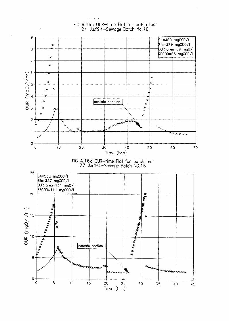
9
8
7
Cl:'. ::::> 0 3
2
0
* =
*
*
*
* * *
* ..,.,..
* I lie
* J * " * * * /
0 10
FIG A. 1 6 c OUR-time Plot for batch test 2 4 Jun'9 4-Sewage Batch No. 1 6
* """
,IE ,I
"" !acetate addition J *
* \. = ' f\ *
* .
1Sti=469 mgCOD/1 lste=329 mgCOD/1 K.JUR area=89 mg0/1 RBC0D=6 6 mgCOD /I
** * *""*-*"· "" "* ..,... . '~ '
20 30 40 50 Time (hrs)
FIG A. 1 6 d OUR-time Plot for batch test 2 7 Jun'9 4-Sewage Batch NO. 1 6
,+
****
60 70
25.....----------.----r-----,-----.----~---~--~--~ Sti=533 mgCOD/1
....--. L
£ '-.._ 15
" 0 0)
E ~
O:'.: 10 ::::> 0
5
Ste=337 mgCOD/1 OUR area=131 mg0/1 RBCOD= 11 1 mgCOD /I
* * * ,If.
* * * acetate addtion
0 -4----4----4---------1------!-
o 5 10 15 20 25 Time (hrs)
I I I
I * * *
*
40 45

25
20
,......... L
..c "'-.. 15
' 0 CJ)
E "-..../
O'.'. 10 ::J 0
5
0
20
18
16
14 ,.........
L ..c "'-.. 12
' i10 E
"-..../
O'.'. 8 ::J 0
6
4
2
0
1 • * ..
I * . .,
IIE
l •
f ~
IIE
* V -~
FIG A.1 6 e OUR-time Plot for batch test 1 Ju1'9 4-Sewage Batch No.1 6
,. :
Jj ~
* ., "" * *
* * * * *
I acetate addtion J ~ *..,
Sti=464 mgCOD/1 Ste=294 mgCOD/1 OUR area=120 mg0/1 RBC0D=64 mgCOD/1
~ ' ~**~ IIE***~ *****~ ~* """'****
0 5 10 15 20 25 30 35 40 45
0
"' * •
~-
lf
* ~ * * I!"
* ~~
* *
l * * *
Time (hrs)
FIG A. 1 7 a OUR-time Plot for batch test 8 Jul'9 4-Sewage Batch No. 1 7
Sti=556 mgCOD/1 Ste=27 4 mgCOD/1 OUR area=224 mg0/1 NOi=O.O mgN/1 NOe=O. 1 6 mgN/1 RBC0D=142 mgCOD/1
~
~ * * ""' * I ' * ..
I/ -~ ""
/ *it **"'***it *-**"' ~ /
---~---->-- - - -- - ---5 10 15 20 ?5 :rn 40 45
Time (hrs)
50
50

FIG A.1 7b OUR-time Plot for batch test 5 Jul'9 4-Sewage Batch No. 1 7
30-,,-~~~~~~--.--~-.-----~~--~~------,-------, Sti=504 mgCOD/1 Ste=359 mgCOD/1 OUR area=164 mg0/1
25 NOi=0.04 mgN/1 NOe=0.02 mgN/1 RBC0D=137 mgCOD/1
..-.. 20 L
..c
" .~ " i 15
* E
" '-"
O:'. * ::J * 0 10
acetate addtion
* * * *
*
0;-----;-----+-----1--------+-----+-----l 0 5 10 15
Time (hrs) 20
FIG A.1 7 c OUR-time Plot for batch test 7 Jul'9 4-Sewage Batch No.1 7
25 30
35~--~--~---.----~--~----.----.---.--~~~~~~--. ti=492 mgCOD/1 te=347 mgCOD/1 UR=2 1 3 mgO /I
30 4-----"'4----+----+----+----~-~----+---l. Oi=O.O 1 mgN/1
25 .......
L ..c:
~20
" * 0 0) * E
'-" 15 O:'. ::J 0
acetate addition
10
0 -+------+------+-----+-----+---------- -
0 5 10 15 20 25 30 Time (hrs)
35
Oe=0.02 mgN/1 BCOD= 1 7 1 mgCOD /I
40 45 50

20
18
16
14 -l '* ~
:' ~ L ..c "- 12
" i 10 E
/ f * * -* * '-../ *
Cl:'.: 8 :J 0
6
4
2
*
* r ,r. -~ -
I/ * * -~ /
/
0
FIG A. 1 7 d OUR-time Plot for batch test 9 Jul-Sewage Batch No. 1 7
* *
'* '"' *
"'
*
I acetate addition *
\ *
~- \ ~,, ~ ~.
Sti=504 mgCOD/1 Ste=371 mgCOD/1 uUR=160 mg0/1 NOi=0.02 mgN/1 :Oe=0.06 mgN/1 RBC0D=158 mgCOD/1
' !iio...,,_, \ =~
"~, ~*~**
0 5 10 15 20 25 Time (hrs)
30 35 40 45
-L ..c
FIG A. 1 7 e OUR-time Plot for batch test 13 Jul'94-Sewage Batch No.17
20--.--------.----------.-------,-----,------------::---, ti=5 1 4 mgCOD /I
*
te=3 9 7 mgCOD /I Oi=0.1 mgN/1 Oe=0.06mgN/I
16 -+------+---w-*----+-------+-----11UR=146 mg0/1 : * BC0D=155 mgCOD/1
,)f, * ,j!.
I' "- 12
* * * " 0
CJ)
E '-../
Cl:'.: :J 0
8
* * 4
* *
* * *
*
* * *
* *
0 -+--------+-------+--~- ..
0 5 1 0 Time (hrs)
* *
, 5 20 25

16
14
12
,,-...
_e 10 '-..._ 0 '-..._
8 CJ)
E '--./
Cl:'.'. 6 ::J '>II'
* 0 )
* * 4 -* * l ~
2
~ -0
0 200
FIG A. 1 7 f OUR-time Plot for batch test 1 4 Ju1'9 4-Batch No. 1 7
~ r)I ~ ~
,ff- ~ , "'
,ZS ~ * )ll~
~ ,/'
* 11,
/ lrJ,
~~ '***~***
/ /
Sti=534 mgCOD/1 Ste=359 mgCOD/1 NOi=O. 11 mgN/1 NOe=0.13 mgN/1 0UR=211 mg0/1 ~BCOD=144 mgCOD/1
~* * * **~--"· -
400 600 800 1000 1200 1400 1600
Time (hrs)

25
20
......... L
..c .........__ 15 .........__
0 O>
E O'.'. 10 :::J 0
5
0
\, =
I * *
*' ~~ * ~
* * ~ * * -
* ~ * * r. * *
•= V
L/
FIG A. 1 7 g OUR-time Plot for batch test 1 8 Jul'9 4-Sewage Batch No. 1 7
1Sti=461 mgCOD/1 1Ste=310 mgCOD/1 OUR=164 mg0/1 NOi=0.00 NOe=0.00 RBCOD= 1 9 8 mgCOD /I
.,.'M.#*
/ * I sewage addition ,I * ~ *
IS
~ * ~ -""""~ * .. ;~ ,,.,.,, llll9I,
0 5 10 15 20 25 Time (hrs)
30 35 40
FIG A. 1 7 i OUR-time Plot for batch test 1 9 Ju1'9 4-Sewage Batch No. 1 7
45
25.----.----,----.-------.------..---~~-~-~------~
20
......... L
..c .........__ 15 .........__
0 0)
E '-./
O'.'. 10 :::J 0
5
ti=486 mgCOD/1 le=326 mgCOD/1 UR=149 mg0/1 Oi=O.O mgN/1
+----w-----+----+---+---1------l---+--NOe=0.06 mgN/1 BCOD=158 mgCOD/1
* * ~ * * l
* * * * * * * sewage addition
**** *****
0 -+----+---+-----+-----1---- -- --- ---+----l 0 5 10 15 20 75 :rn ~~ 40 45 50
Time (hrs)

45
40
35
..- 30 L .r:
' '- 25 0 CJ)
s20 a:: ::J 0 15
10
5
0
18
16
14
..- 12 L .r: "--.:::::._ 10 0 CJ)
E 8 '-.../
a:: ::J 0 6
4
2
0
....
• ,. I • f I f * I
I l
.w ~r
I } " lE
I ~
* * ~ /
0 5
:I.Iii:
* * *
l
~
* * ~-
*
FIG A.1 7k OUR-time Plot for batch test 21 Jul'9 4-Sewage Batch No.1 7
; r; !sewage additon I
\ y "'
·~
$ti-51 B mgCOD/1 Ste=392 mgCOD/1 OUR=219 mg0/1 NOi & NOe=0.00 RBCOD=2 3 1 mgCOD /I
·~* IE****** **
10 15 20 25
Time (hrs) 30
Fig A.1 Ba OUR-time Plot for batch test 29 Ju1'94-Sewage Batch No.18
35 40
Sti=451 mgCOD/1 Ste=269 mgCOD/1 OUR area=177 mg0/1 NOi=O.O mgN/1 NOe=0.07 mgN/1 RBCOD= 1 0 0 mgCOD /I
~ f,; ~ "" * I
,,,
* * * ""' ~.
* V -~
f** * / /
0 5 10 15
* **** ""****** "" *** ~ .... *
20 -
75 Time (h,s)
-,:r, ,,•1
"-~" ~ ·~
- -
~** - - .
40 4'.i
45
50

22'
20
18
16
....... Eu
' "'-.. 12 0 CJ)
E 10 '-./
O'.'. ::) B 0
6
4
2
0
25
20
5
0
= ,z. w
* * * * "" II
* * * "" * = ~~
* " w
I * ~ * * I ' I
FIG A.1 Bb OUR-time Plot for batch test 25 Jul'94-Sewage Batch No.18
S1i=469 mgCOD/1 Ste=282 mgCOD/1 OUR=176 mg0/1 NQi:::;0.23 mgN/1 NOe=0.30 mgN/1 RBCJ[;~ 126 mgCOD/1
~ !sewage addition I ,
""
\ I"'
"""' ~ ~ ... '~~ ~
~** i..:-~
""'**
0 5 10 15 20 25 30 35 40 45
I =
Time (hrs)
FIG A.1 Be OUR-time Plot for batch test 26 Ju1'94-Sewage Batch No.18
S1i=4B 1 mgCOD/1 Ste=334 mgCOD/1 OUR=239 mg0/1 NOi=0.39 mgN/1 t.JQe=0.21 mgN/1
50
~ RBC0D=144 mgCOD/1
* * * * * * ""
~
* * * * *
* f, * * : '* ,.;t,i. *"""'"
[/ ~ ~ -* -.....'ME """' - "'·=· ···~
~**')I ~
******~ ** ---------- ----~-->---
0 5 10 15 20 25 .~O AO 45 50
TimR(fYs)

22
20
18
16
,,-....
1: 14
' '-..... 12 0 0)
E 10 '--/
Cl'.'. ::J 8 0
6
4
2
0 0
22
20
18
16
,,-....
1: 14
' '-..... 12 0 0)
E 10 '--/
Cl'.'. ::J 8 0
6
* 4
2
0 0
* llE'
* * ~
*"" /'
FIG A. 1 8 d OUR-time Plot for batch test 2 7 Jul'9 4-Sewage Batch No. 1 8
* *
~*
; "" • . .lf-
II<, * *
* - !sewage addtion , f~
, '*~ ~ /
$ti=545 mgCOD/1 5te=361 mgCOD/1 NOi=0.03 mgN/1 N0e=1.64 mgN/1 PUR=175 mgN/1 RBC0D=159 mgCOD/1
~f - "' * - ---
* *
* •'
r
'"" *****~ ~ / - )IE>l:)I *
·' , ~
..... ,, ,,.,•"
~,.·' .•.
it ~
* * ""'
f ~~
I ~ * * *
""' * * *
= * * * *
5 10 15
Time (hrs) 20
FIG A.1 Be OUR-time Plot for batch test 2 8 Jul'9 4-Sewage Batch No. 1 8
* ~ * *
V ' ~ ~ .. ~
/ = ~-II!
/ ~ "" ~ ~ ""
..
f-- -~-·~-- f- - - -
5 10 15 20 75 :rn Vi Time (hrs)
25 30
Sti=555 mgCOD/1 Ste=334 mgCOD/1 OUR=219 mgO /I NOi=O.O 1 mgN/1 NOe=0.08 mgN/1 ~BCOD= 1 6 1 mgCOD /I
~
- - --
.10 45 50

FIG A.18f OUR-time Plot for batch test 4 Aug'9 4-Sewage Batch No. 1 8
25~-----,~----,.,-----,-----,------,-----,---..,.....----r--------:--::-:---/;:----, i+, i ! , 1 ti=503 rngCOD I ~ i 1 1 1 te=260 rngCOD/1
j I I i I ~:02~: ~/: 20 ................. Et·····················t··· ·················t .. ········--····--····r··----············· ; ........................ ; ............. ········1.··--········ ~i~~~~738rn~~0D/1
! : i i * l l ! l ;,,:':. ,,.!
: 1, 1,. : : ! : j : ,,-...
L
~ 15 '-,.
···········t······················· :
I 0 CJ)
E '-..J
Cl'.'. 10 ::l 0 ·~· i
·······1.· ····+······· ············r·--··--······ ··
i l . . ! . .
... ,~. ;··· ····r 5
. * i *i
0 +---+--------it-----+---+----+-----t----+----t-------t-----l 0 5 10 15 20 25 30 35
Time (hrs)
FIG A.18g OUR-time Plot for batch test 5 Aug'9 4-Sewage Batch No. 1 8
40 45 50
25.-~~~--,-~~~--,~~~~--,-~~~---,-~-,-~~~~~~
~* '·!,!,,, !~==~~~ :gcc~t1
Oi=0.00 rngN/1 Oe=0.02 rngN/1
! : : ....... J .............. 1 ...................................... 1 ...................•••.•• ·········· 1·········· ····•·••••••••••• r...... ~~~~~f2~g::~I .. 0 * * CJ) * E * 1 1 i 10 :····························'·······································(·························· ·········································
I sewage addition
r····--·· 5
0 -+------,-------i-----~--i-- ·t·
0 1 0 20 30 40 60 Time(hrs)

..-...
FIG A.1 Bh OUR-time Plot for batch test 6 Aug'94-Sewage Batch No.18
25~-**---~---~---~-----,-------,',:,::'..--.:-~ti=~5~1~1:---m-gC~O~D~/~I-,
te=297 mgCOD/1 UR:: 247 mg0/1
* !· i Oi=0.00 mgN/1
20 ;···· -1-----i----r-·····1······1············· ~~g~~~ :f/~/1 L
..c. """- 15 :. .... .'............. .. .................. ..1 ..................... 1.. ......................... !... .......................... .
* ; j i " 0 0)
E '--' Cl:'.'. 10 ::J
:· ... It :······························ 0
..-... L
..c.
5 ................. : ....•... ~········
j* O-l------+------+~-----+----+------+-----M1----1 O 10 20 30 40 50 60 70
Time (hrs)
FIG A.18j OUR-time Plot for batch test 7 Aug'9 4-Sewage Batch No. 1 8
25-,-------,------,----~----.,-------,----,-------------,
* *
Sti::51 0 mgCOD/1 Ste::251 mgCOD/1 OUR::264 mg0/1
Oi=0.00 mgN/1 20 ............... 1 ........... ··:···················· r ··-········r······························+······························· 1··········· :~~g~~~ ~~/I
ft * * * *
"""- 15 ·············+·····························1··············· ···r·························· ·····:·· ..... ····t ·········•·························· """ 0 0)
E '-../
Cl:'.'. ::J 0
10
5
................. ·+ .................... '"!"' ! ,t 't"' .......... .
.-s-ew~a-g-e -a-dd-it-io-n..., I *
j i
* : ~
·········~, ........................ [··• .................. .
j~ : :
0 -+-------- ---r~~ ~--+--- · t -r- -----------i-------1
0 10 70 30 4~ 'in 50 70 Time (hrs)

FIG A. 1 9 a OUR-time Plot for batch test 1 8 Aug'9 4-Sewage Batch No.1 9
30-r----~---~---~-----, ---~--------,------,
1.. I 25
r-.. 20 L .c ''i 15 E
Cl:'. ::::, 0 10
5
! ·-···················+····-····························+··································
! i : !
i j j j
! ! ! : : : : : i
I i i i i i .. * .... : ... :.,····· ................ 1.,,.. ···················:·!·.,· ! Lj I ' '····,~\ .... ) ............................ .
* . . .
~i i ~****
O+------t--------t------1----+-----+-----+---------1 0
40
35
30
,-....
£ 25 '-'-i20 E ~
Cl:'. 15 ::::, 0
10
5
10 20 30 40 50 60 70
, Time(hrs)
FIG A. 1 9 b OUR-time Plot for batch test 13 Aug'94-Sewage Batch No.19
········t· ; ···························· ·······························(··························· ............................ .
;A I r···· r · r
ti=5 3 4 mgCOD /I te=321 mgCOD/1 UR=246 mg0/1 Oi=0.35 mgN/1 Oe=0.00 mgN/1 BCOD= 1 3 0 mgCOD /I
rr······················1 :······························ ··r························i
···················· .....• ·······························r··········· ···········:············· ........... ,................ ··r·········· ····t ............................... .
···········•················· ·············+····························:············ •••;••• ··············\·····. ·····1
··················--········'"·--·-·························t··-···························1 ····i
~i .. ·····--·~- .................... ·········t ································
1 l .
0 -+------+------+------+- -1 --r-60 0 10 20 30 4[; 70
Time (hrs)

FIG A. 1 9 c OUR-time Plot for batch test 1 5 Aug'9 4-Sewage Batch No.1 9
25.....-----,-------,----.,--~~..--~--,-------,-------,---,-~~~~~-,---,
J,,. ~** I I._·. ~~~{ ~Jifil ** i BCOD= 1 2 0 mgCOD /I
2 0 ....................... ..;. ....................... ,t ..•.....••.......•..... ; ............•••.••••... 1 ....................... 1 ..•.•....••..•........•.•.......•.........•... 1 .................. ----~---····················+·-·····················
; i ** !,,, i,,. !... !,.. I I I ,,-....
L
..c 15 '-.. '-.. 0 CT)
E ....___, CY 10 :::)
0
5
1: · · · · I I I • ~ 1 1 l ! ................ , __ ..................................... . l * I I I l I ! ! ! . * . . . . . i ! '. * '. ! ! ; 1
: I I ·········~·~=~·············· , ....... ····· r······ 1 ·· -~~r···· ·········· :········ ······ +············· ·····r······················r··· ···········
- l**- : "' : "'* . -·1.· ·+· ..... (_ .............. _ .. ! ....... ~***~+;~-------= 1 · .... = .. .. I i *"'l*****
0--r---+-----+----+---+---r-------t-----+-----+---+----l
0 2 4 6 8 10 12 14
Time(hrs)
FIG A. 1 9 d OUR-time Plot for batch test 1 6 Aug'9 4-Sewage Batch No. 1 9
16 18 20
35-.----~---=.,-:;,·. ~~--,--~~--,---~~~~----,---,--~~~~-, l1le ti=545 mg COD/I
n.,.,_ ...... ___ .... __ ...... _ .. _ .... i ................................. i:,,_·:,,··························· ···················· [ ~~!~~.;~;:/I ;; ; ; --·-······!_;',.-· \ BCQDa 114 m~~/1
30
25 ,,-....
L ..c ~20 '-.. 0 CJ)
S 15 CY :::)
0
..... ,-.... ; .. - ......
* ; . : ' : .... -).1( ........ L .... -....
* * I : .. , .... ·+·
* I : 10 ......... ., ....
l ~
5 ... , ....... _ ... ______ t
---.- .... !... ! t ' i·· ························
l~ * *
i* ···················t······························-···1····················· ········+························
l :
O-+------------+-----t-- -t- -t
50 0 10 20 30 40
Time (hrs)

FIG A. 1 9 e OUR-time Plot for batch test 1 9 Aug'9 4-Sewage Batch No. 1 9
40-.-----,,------,-----,----,--------,-----....,......--------~----,
35 (* ! ; ; . I ~~W?f;!1
! ~ I I Oe=0.01 mgN/1
"'""..cc :: ............... ·······1: ~ ·1············· ·· 1·····························1························1 ························· ... !,,,:,:,, .. ::=123 mgC00/1
" : * i i i ....... :........................ . .................................... ..
~ 20 .......... fr =············I · . ·l·····························i··· ····················i·····························:·····························i···························
s • i i i ~ 15 ............... * .......... : .............................. : ........................ ....!......................... . .................... , ...... .
O ; ~ I . I sewage additon
10 ·-J'······ ........ ; ... \l·· ; ! ·········~,.····· ············ ~· * ! ~ i \
t : ""l'!r'4""'""~'"''~'"""'~'. .. '" ~~-· ··< . . ........ t .................. . 5
0-+----t------t-----+----t-----+-----+----t------i
0 5 10 15 20 25 30 35 40 Time (hrs)
FIG A. 1 9 f OUR-time Plot for batch test 20 Aug'94-Sewage Batch No.19
40.-------,-------~-------,--------,.------.--------------~
35 ......... J ...... •. · ' !· ... ... i : ........ . . : . .
30
ti=579 mgCOD/1 te=319 mgCOD/1 Oi=0.17 mgN/1 Oe=O. 1 4 mgN/1 UR=297 mg0/1 BCOD= 1 8 0 mgCOD /I
i 2 s J : ! ......................... I . _ j20 ~= ; i ; · ·················· ······································
'-../ . ~ 15 ·*·· ······*····· ......... ; ········· · .. . . · ·
0 * I ! sewage addition 1 0 * · r\ .. +........... . .... ; .... · ...... i .... · ... J.t.. .... . ......... .
~~~,.~-L. ... " r,. 0 -+-----;---------i--------r-· -
0 10 20 30 Time (hrs)
- r-40
-r--50 60

-. L
.r::
Fig A. 1 9 g OUR-time Plot for batch test 1 6 Aug'9 4-Sewage Batch No.1 9
35~---,----=-,----------,----.---,----,----,--,-~-,--~~--;-~--, ti:=545 mgCOD/1
30
25
le:=346 mgCOD/1 UR area==243 mg0/1 Oi &:NOe== 0.00 mgN/1 BCOD== 11 4 mgCOD /I
........ ! .... ! i !
':::::- 20
" 1 I I
.................... . = ....... llE.. i *
0 CJ)
E "-../ 15
I' :, ....................... :·* ............ ..
11 *rrrr 1 r r
-.
10
I : ... ,t--.............. . -r- i
5 '¥l *
'~J+ 1 .... ,
----i=,=.··-·· ---··+ ---·········{········ --······i···· --··· ---·······-r-····· ···············1_· ......... .
',.·=,,. : ~~~
0-+----+---i----t---+---~----+---+---i----J----l 45 50 0 5 10 15 20 25 30 35
Time(hrs)
FIG A.1 9h OUR-time Plot for batch test 2 3 Aug'9 4-Batch No. 1 9 (I)
40
40-,--------=,,---------.-----~-----,-------~ ti==420 mgCOD/1 le==362 mgCOD/1
35 +----------'l~f-------+------l------fJUR==2 2 7 mg0/1 Oi==0.36 mgN/1 r Oe==0.03 mgN/1
30 -t----~-t-------+-------1------1 BC0D==126 mgCOD/1 ~ ,
£ 25 -t------:-;;r---t-------+-----+------1------_J
" 0
" 0> 20 -t-~*.:------1-------+-----+------1------_J
E * ~ 15 ti~----E------+-----+-------1------_J 0
0 +------------:f-------+--0 5 10 1 'i 70 25
Time (hrs)

FIG A. 1 9 j OUR-time Plot for batch test 25 Aug'94-Sewage Batch No.19
::~---.-..... -.... -..... ~ ... :~:-..... -.... -.... ---:--*-... -..... -.... -..... -.... ~l-..... -.... -..... -.... -..... -.... -.... -..... -.... -....... j-.... -..... -.... -.... -.... ---.-~i-~~i~~~~7~-~-~~~~l~f~I/-I-,
i * i i BC0D=1 OB mgCOD/1
25 ···················· ,,-,...
L .c ~20 '-...__ 0 O>
E .._ 15 0:: ::J 0
10
----··········-······ -·-················
···················
* ···r ~ · 1··· · t / : * ! .
5 .:. ........ . ····················· ' ~-····f *;!'.•ii~-~-.. f • •• ,. ... ,.. 0-+-------i-------+------+------i-----------i
45
40
35
,,-,... 30 L .c '-...__
"'- 25 0 O>
E 20 .._ 0:: ::J O 15
10
5
0
0 5
)
* * ~
~ * )MIE
* ~
"'~ * .,,,.
..A<
t /
10 15
Time (hrs)
FIG A.19k OUR-time Plot for batch test 28 Aug'94-Sewage Batch No.19
I'*-
* * ~
. ........ill.< *~ .,,., V *
)~-
20 25
Sti=5B4 mgCOD/1 Ste=260 mgCOD/11 OUR=2BB mg0/1 NOi=0.04 mgN/1 NOe=0.07 mgN/1 RBC0D=9 9 mgCOD /I
= = - ~--*=
- --- - -
0 5 10 15 20 25
Time (hrs)

FIG A. 1 9 m OUR-time Plot for batch test 30 Aug'94-Sewage Batch No.19
30-T----------,------,----,-------,----,----,-~~~~~,---, ti=5 6 7 mg COD /I te;;:344 mgCOD/1
ti UR=202 mg0/1 25 ·············;*:········· ·········1··········· ·······t···············i······················•············ ········: ················1 ~~:~~¥~D/I
s * i I* ; ~ .. ·········· ··········· • sawage a:i;: i ... .. j• Ct'.
:)
0 10
5
:* i i I i r~ J\ ·········'r~~L~j····· . 0+---+----+----+---+---->----+----+----+----+----1
0 5 10 15 20 25 Time (hrs)
30 35
FIG A.20a OUR-time Plot for batch test 2 Sept'94-Sewage Batch No.20
40 45 50
35~----------------------,---------, ti=606 mgCOD/1 te=283 mgCOD/1
30 ................ ~.-····· . . . ... . UR=339 mg0/1
f. l ! / ~~:~~~OD/I 25
,,-._ L
..c
~20
" 11: , i i r t r
. ~ ·i ............•.....
··················1·········
·················1·······
0 CTI * * * S 15
~ ······* ....
* * r-·Jlf .......................... .
Ct'. :)
0 : *
10 * ···-········t··· ··········t···· ~i;:
=~-I:= ~ ...... -~ - { '¥.•,-,.,. .• .,. •i.-.,,.., ...... ~->!('+,
········1·····
0 -+----.-----..-----;.------j------- -,--- ·1- -r- - r 0 5 10 15 20 25 30 35 40 45
Time (hrs) 50

FIG A.20b OUR-time plot for batch test 4 Sept'94-Sewage Batch No.20
35~---.,------,-----,-----,-----,-----.,,...---~~~~-, • , li=526 mgCOD/1
! _ _ le=309 mgCOD/1
30 ------------------------------l-------------~-----1------------------------------1-----------------------------l-------------·-··--···-·-····l····-------------------------! g~i~~ ~~~;: ! • ! i ! i i Oe=O.O mgN/1 : * * : : : : : i * i i i ! i BC0D=132 mgCOD/1
25 ·---------------------------·:--------,Jt--------*----J------------------------------:------------------------------1·----------------------·-----·1·---·-----·-----·-------------1--------·------------·-·-----!-------··----------------·---
~ : * *: : : : : 1
.r: i* *i i I i i i ~20 '-0
O>
E '-../15 -----·-------· ·------···----
sewage addition
10 ............................ i ............................ ~
5 -·-
r :·······················1 ; r························
O+-----t-----t-----+-----+----+----+-----<e--------1 0 5 10 15 20
Time (hrs) 25 30
FIG A.20c OUR-time Plot for batch test 6 Sept'94-Sewage Batch No.20
35 40
25~----------------------~------~ li=5 2 0 mg COD /I
.......... L .r: '.. 15
'-0 O>
E O:'.: 10 :::, 0
* : : j i * ! * ! I ,
* * * ............................................... * : * * * * * *
--- --- --+·--·---··---- r ~- !
5 -·-*-----*
* "" : ······-····-*············~::--··--········-·····-·-·-·····-i-----·····---·-·-··-----···--·---··--·
* ~ ,,., ** ; ***
* ***
0 -+------+------+-------r-· 0 10 20 30
Time (hrs)
- t·
lO -r- _____ _, '.>0 60

FIG A.20d OUR -time Plot for batch test 7 Sep'94 -Batch No.20
30--r---.,...------,,-------,-----,,.'.:--,i,-------,---,---r-S~ti=~5~2~0-m-g~C~O~D~/I:-----,
i 1,,,,. Ste=297 mgCOD/1 * , OUR area=259 mg0/1 l . . 25 ...................... 1,,,,.- ~ .. ;--.............................................................. 1,,, ................. + ...................... t ......... ~g~=OO~O;i~~/1
* ! I I : I RBC00=140t:~I-
....-... 20 L
..r: '-.. 0
cii 15 E
O:'.'. :)
0 10
I l I
.. i i - ' : : I I I . /I I . . I
sit ·:~d r . . 1*****lt *
! i 0-+---+---+----+---+-----i,-------+---+-----r----r----J
O 5 1 O 15 20 25 30 35 40 45 50 Time (hrs)
FIG A.20e OUR-time Plot for batch test 8 Sept'94-Sewage Batch No.20
18-.-----,--------------------~--------. ti=543 mgCOD/1
. . te=309 mgCOD/1 16 ·················· ' ........................ , ........................... ; .......................... ,............ ··r ·· ·· r ·· ····· UR=296 mg0/1
14
....-... 12 L
..c '-.. '- 10 0 CJ)
S 8
O:'.'. :)
0 6
____________ ...... T .... #
: * i i i ......... i',, ... lM'E .... . ...... Jl'.. : : . /1- .. ,.. .. .... ,............. .... . ..... :~
~ i ~ ................... }1(.i .......................... : ........................... : .......................... :........ . ........................................ .
/ ' i !- : j ,,_wage ad<ilioo 1 ~ * * i i
.: ~ i ;~ .. : 2 ; r j .. ....... 1 . . .. . • . ..... ... ! •.
0 +-----+----+------+------+---+-------r-----+--------<-----<
o 5 10 15 20 25 .~o 40 45 Time (hrs)

FIG A.20f OUR-time Plot for batch test 9 Sept'94-Sewage Batch No.20
25-------------....---,-------,-----,----,--------------::-,
I I ~il!f!bi~11
20 -- f tl., 1 ... ·-················1.i······················r-············+············ ·r········· ~;~\\~~;,
! 1s ............... , .... f ~L- ..... L-- .......... J ...................... , .................
1
.. ·······)········ ............ 1 .......... \ ........ .
E
O:'. ::J 0
* : - \ \ * i -~ . . * . '* 1:1' !lo!E
s/' /.,,~···············' ......... J ........... +• * ~ ;
: j
0 -+----+--------i----+-----i-----i----i---t----t-----t-----j
0 5 10 15 20 25 30 35
Time (hrs)
FIG A.2 1 a OUR-time Plot for batch test 1 9 Sept'9 4-Sewage Batch No.2 1
40 45 50
20.------,----,-----,-----,----,------,------,---,--------------, Sti=583 mgCOD/1
· te=330 mgCOD/1 18
: + r r 1 r 1 1
°'6;~026; ~~~:
:: J + t t l 1 1 ·· r ·~~~~g~~~ ~~/I
* i i ................... ; .................. :
*
8 ....... \ ...
6
4
2
~--··· ·····-······t·········· ···········t··················-···-~-- ·--·················t·····--················i ······················t ..................... t······· ··············1· .......... ·.·.·.· ..... ·.·······:.!:,: ·.·.·.·.···················
. i ' .... ,.. :. L T ....... -
I i ·: .................... t .................... t .................... r ............................. 1 .. --· r ······ .. l .. t
- ! (··············•············· •······)}
..... ~! ~·~·············~·······~······
0 ---r -1-
0 1 0 20 30 40 50 nO 90 100 Time (hrs)

FIG A.21 b OUR-time Plot for batch test 21 Sept'94-Sewage Batch No.21
12 ~--*-!,,,.-.---i.-------i----1
.,.---~-t-i=-5-83-m_g_C_O_D/_I __
:,, ·.:':, te=291 mgfCOD/1 : \ UR=246 mg0/1
1 0 .................. *. ....... L ............................. L ............................ L. ......................... ·.,i .... ·· ............. ·········L. .......... ············-r-- g~==OO ~71 ::ti I I I , I BC00=99 mgCOD/1
,,-...L 8 ........... * ... : ............ .!,,, .............................. !,,,···················" ....... ..!,,,······························:,i.·· ! ........ • ............................. i ............................. . _c 1,. 1 1 ' .,: ··' .,,: .,: ! ! -" : i i: ~ 6 ····;t········· J ........................... [.* [ .............................. \ ............... ············!······························i························t···················
: 4; f~ I i .~w~a:H: /\._:: ... ; I
.... ·+··············· ... r·········· .. ····1······················1······· :···········
O+----t-----+----+----i-----+-----+----i------j 0 10 20 30 40
Time (hrs) 50 60
FIG A.21 c OUR-time Plot for batch test 23 Sept'94-Sewage Batch ND.21 (L)
70 80
16,-----,------,---------,------,---------.-----,-,---------, ti=5 1 1 mgCOD /I te=244 mgCOD/1 U ?*T i i i ···················································· ::{~}1 ;I
1 2 ............. )tL. . .. · · · .. . . ·····r···· .... BCOD= 11 2 mgCOD /I
E : .... * ··1····················· . ·········- ... ~j ..... '-.../ :lfEi *; !-l ....... (·············· ..... ... .. . . ·······: sewage addition
~:.L~~~ .. I.. .. : ............... .1. ............... . I .
~ 6 : 0
4
····················;·-··
2
·······················r~ ."."""'**',"""'··· *****: i··
O+----i-----j-- -~-+-- --··--·-t· -t --+------, 0 10 20 30 .10 r; (; 70 80
Time (h"s)

FIG A.21 d OUR-time Plot for batch test 23 Sept'9 4-Sewage Batch No.21 (R)
30~--------,--------,-----,-----,------,-------,----,------------:----, I 1 ti=511 mgCOD/1 ; 1 Ste=303 mgCOD/1 i i UR=211 mg0/1
25 ............. t' .... f .............................................................. L.. ................ j ................... ,l. .................. l.. ..... Oi & noE=0.00 mgN/1
} I \ I I I I I RBC00=107 mgC00/1
,........ 20 L
..c
' ' 0 15 CJ)
E '-,.J
Cl'.'. :::i 0 10
*
..... .. r·· : ... . -· ... ; ; sewage addition i *
: : i *****~***
~~~--;~: .. '* .. >te4E*.ij,!lj! .... *' .... '* ... ~l·;;;·;;l~~·I~~~:~~[ .... T. ····· ..... !,:,.,:', ..... :;;;;:· ..
0 +-----+----+----+---------! ___ · ---+-! ----+-' --------0 5 10 15 20 25
Time (hrs) 30 35
FIG A.21 e OUR-time Plot for batch test 2 7 Sept'9 4-Sewage Batch No.2 1
40 45 50
18-r-----,-----.,...--------------------~------------~ ti=556 mgCOD/1
15
-... 12 L
..c
' ' i 9 E
Cl'.'. :::i 0 6
3
~ ! ~e;!~~t~~~~I t 1
, o· 0 1 0 N/1 f ·················· · r I + r ~~~1111 ;~~OD/I
! l• ·······························I ············1··························; ·····;···· ·•··························
·····** ............. -........................................... 1 ...................... 1 .......................... .
* * *
·---············-···············
* . / . :
~L-=t:-r~+···~t~~-* .. L· 0 +------+---+------+---·-+--- -i--
0 5 10 15 20 ?5 40 45 Time (hrs)

20
18
16
14 -.
L ..c
FIG A.21 f OUR-time Plot for batch test 2 7 Sept'9 4-Sewage Batch No.21 (L)
/ , ti=556 mgCOD/1 * ! ! le=351 mgCOD/1 ................ 't" ........................ T ................................. , ............................ r: .......................... , ...... g~=o1.~6 ~~~~:
......... ?··)·············· ···············r························r·························r ··························· ·r······· ~~~~1,~ t~OD/1
i i i l l ·!,, ................................. :.: ................................. ..
'-.... 12 ~ !. !. : ! ............... ; .................................. i ................................. J ................................. .
.... i ..................... J, !, !, ............................ I I I '-.... i 10 E ~
.. : l, \
: i i i O:'. 8 ::::i 0
6
•················· r············· ················r·-····························l················ ·+············ ·······.· ....... l,.;. .... 1 ····· i ....................... ...... . . . ................ ,; ...................... .
~ sewage addition
4 .; ......... . ········-···; ····---·---···············-·{---- .... ---····-r··· -----·····;······-----·
2 ·············-·····f-···· ............ 1···· ......................... .
O+-----t------+------,>-----+-------+------+-------1
0 10 20 30 40 50
Time (hrs)
FIG A.21 g OUR-time Plot for batch test 30 Sept'94-Sewage Batch No.21 (R)
60 70
16.--------,-------,-------,----~----,----,--------, * Sti =523 mgCOD/1
S1e=346 mgCOD/1 14 ....... * .. ····· ......... _ ............................ ; , ........
1
;- .......... OUR=213 mg0/1
• [ I Ng~ci~01 ':.01
~ :: ·~············ .•.•.••••••••••••••••••• , 1 .............. ···················•··•·•··•••·•·•·•·•••·••·••········ ........ RBC0D=97··=~~I.
'-.... * i 8 . E . : : j
~ 6 ........ ..
0
.. .......................... , ................... .
42 .••..••••••••••••.•.•••• ~ .... ~ ....... -.'.,.'··································.-................ 11. .L~ .......... :··
*
0 -+-----+-----+----r- .. -- · -1
0 10 20 30 ,H)
Time (hrs)
·······························-}···· ························
. 1
:; ()

20
18
16
14 ,,-...
L
FIG A.2 1 h OUR-time Plot for batch test 30 Sept'94-Batch No.21 (I)
i * ! Sti=523 mgCOD/1 • . . ! . !
_:_1.. __j ___ --'-- ... 1............... J_ ~~i:~5~m!~~~/I * : : ! ! ! NOe=0.01 mgN/1
RBC0D=97 mgCOD/1
~ 12
* *
0 '-.... 0> 10
* *
E ~
Q'.'. ::)
0
8
6
4
2
~- ~ I -11- I J J I I ................... , .. ( ........................ ! ...................... 1 ....................... \ ........... \··· ! ... , .......... ;. ........................... .
1 ~. ! ~ . ,.~: : ........... 'i........... ·················· :. .. ****~_***** !
I 0-+------+----+------f----+------<>------+----+-----<
0 10 20 30 40 Time (hrs)
50 60
FIG A.22a OUR-time Plot for batch test 1 2 Oct'9 4-Sewage Batch No.2 2
70 BO
30-.----------,,-----------------~------~ ti=6 6 7 mg COD /I
I * I ~eR==419922 ~io/1/1 25 ........................................ f ..... *................ .. .... .i ................................................ ;................................ Oi &NOe=0.00 mgN/1
i 20 ............................................ ,·.......... -1······················ • BC0D=137 .. ::/I···
'-.... * ' *i ...... * ! i 15 ................ ;..+ ... .................... .................. ................... .. ................ . ...................................... .
; 10
- // ! --y--1 t . ! -
5 ·*" ~ i .J..,,-.. *............................. . . t .. . . ***'***''''"'"**~~ ...... t .................... .
0 -t-------i--------+------ - -+--- .. 1 ~ 0 5 1 0
Time (hrs)
-i-----·----<
70 25

FIG A.22b OUR-time Plot for batch test 13 Oct'94-Sewage Batch No.22
25~-----,-------,------,---------,------.------....,....---, ti=664 mg COD/I
20 ........ ···················:--t-··············· ~!
: I
;I ' !
·-·-··········· ---~ -- ..... ··········· ....
I
te=456 mgCOD/11 UR=2 7 4 mgO /I Oi=0.30 mgN/1 Oe=0.29 mgN/1 BC0D=123 mgCOD/1
i i ! i
J 11
~ 10 :::i
* ··········*··
** It ; -1······!·· ··································
0 * * * * * * 5 ......... .; .... .
*
* j * ; ~ ~
04-------+-----+------1--------+-------+-------l 0 10 20 30
Time (hrs) 40
FIG A.22c OUR-time Plot for batch test 17 Oct'94-Sewage Batch No.22 (raw)
50 60
50.------~-----:w~-------,-----,---------, £1 Sti=1326 mgCOD/1
40
,,.....__ L
_c """- 30
"""' 0 O>
E ~ 20 :::i 0
1 0 ··················
* i Ste=1220 mgCOD/1 * , OUR area=3 1 2 mgO /I * j * l NOi=0.30 mgN/1
1····· ... ··········1·······-r············· ········· ! . ~~;;~~~931m~;0D/I
* ' I * '
·········1 r I I-
·····+····· ············!···· ..
0 -+-------+-------r--~- - ·t ·t·
20 0 5 10 1 '.i
Time (hrs) 25
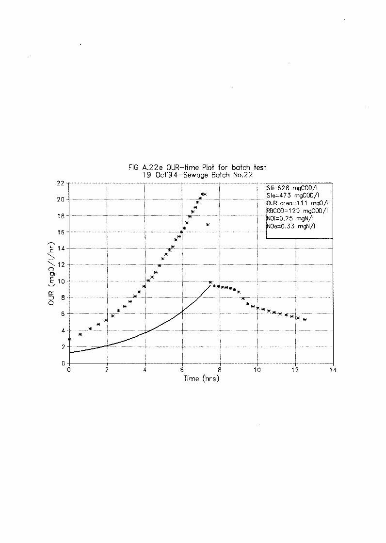
FIG A.22e OUR-time Plot for batch test 19 Oct'94-Sewage Batch No.22
22--r------,------,---------,-----~------,----,,--~~~~~~--. Sti=628 mgCOD/1 Sie=4 7 3 mgCOD/1
20
18
16 ,.-..,,
i: 14
"' "-- 12 0 0)
E 10 '---"
0:: :J 8 0
~ ...... :11::
* * *
··· ········ ····· · -· · OUR area=111 mg0/1
RBCOD=120 mgCOD/1 ' ................... : ······ NOi=0.25 mgN/1
:* i* * NOe=0.33 mgN/1
r····· ··----·····! ... : --:11r·
............. ··--t ··········· .............. , .... . --·~,------· . . :·· .. 1--~---------i ....................... + .................. , ..... +·········· ................. .
i ,,,,/* i --·····r· :*··--···········+···· ···+·-- ........... ,..... ·+·
.... .!.·-* ......................... .' ........... .. "" .......... * ... ' * : *~****
..................... ··1··
*: : : * ...................... - ....... .............. JI! ....... ' .................................. '.............. .. ......... * ....... . * * ** ! ; l!"** ;
·+ ···············:,,· ... *·*·*i.it:· ........ . : ·1
. * .. r * ............ . 6 ........ .
r* --·--:· ·t··· · .. --------·--r· ······------------- -4 ... ; ... ·················--·····1
~ * ·····*
2
*
I i 0---------------------------------<
0 2 4 6 8
Time (hrs) 10 12 14

FIG A.23a OUR-time Plot for batch test 21 Oct'94-Sewage Batch No.23 (3 days)
20.------------------.,..--------,--..-~~~~~~~--.
: I !,, i~R =~ii~m~i~fgfi' ~ ! NOe =0.01 mgN/1
i 16 r ; \ r r r I r :oo~·t~~i~D/I
~ 1 2 : r I 1 t i I,,,,·········· ), r 1, ........ ---·
1 ' \ \ ! ~ s ·-·-----: ............ -... -... +.-... -............. 1 ........ _.-......... l ........ --·-------- ·: ............... _ ... -t--· -·--···- .. -·-·t ·-----·-·--r·- ........ -.... .
4 ········r * . : : : *~*****~*****~****~*
j ) ) ) 0 -+-----+-----+-----+---1-----+------+-----+----+-------->--------l
0 10 20 30 40 50 60 70 80 90 100
Time (hrs)
FIG A.23b OUR-time Plot for batch test 21 Oct'94-Sewage Batch No.23 (4 days)
20.----*----,------,-----,-----.,..----,----,~----~-~--,
t . I 16 ___ .. _ ............... ,_ .... ;- ...................... _ .... ,;-.... -........................ ; .... -............ -............ ; ......... -.................... ; .................... .
I I ! 1
1
,,......_ L
..c: '-,. 1 2 '-,. 0 O> E 0:: 8 :::J 0
= !··················· r r························1.-* : : \\t' +··············1··········· l
*! !* *
····i ············-···············;
0 -+-----+-----+----\-~- -- - "t - I
0 10 20 30 AO 50
Time (hrs)
SIi =561 mgCOD/1 Ste =290 mgCOD/1 OUR =283 mg0/1 NOi =0.07 mgN/1 NOe =0.25 mgN/1 RBCOD=90 mgCOD/1
········,···· ·····!·······
······················l .................... .
I 5 Cl
-r-----------1 70 80

FIG A.23c OUR-time Plot for batch test 3 Nov'94-Sewage Batch No.23 (2 days)
16~----,-----,-----~----,-----,---,.-~~~~~~--,
* \ !,,. ti=5 3 9 mgCOD /I
14 * l te=275 mgCOD/1
* i i i i . i g~:g_-,1~ :::fi1
1 2 ······················ : .... '. ............................. )................. . .. ' ............................... :............... .l BCOD~1r1 ~~~~I
~oL10
E; i. 1························· I i tJ) 8 ................... * ........... :..... ......... . . .. ................... .. s : : I i : i" ~ 6 0
* : . .. ......... i#. * : ! : ~* ; sewage addition J *
4 ........ * ... .................... !"' ................... ··:..... 11*
I*;.~ ~~~-~N~= " ... : ~~~~~ 2 * *
i **; i i ** : *** O -+-----+-i ----+-i ____ : ____ _,_' ----+-----------
0 10 20 30 40 50
Time (hrs)
FIG A.23d OUR-time Plot for batch test 3 Nov'94-Sewage Batch No.23 (3 days)
60 70
2s-.--~~.,---,-----,-------,----,--------,------,.,---------. ti=5 3 9 mgCOD /I
5
* * te=266 mgCOD/1 Oi=0.11 mgN/1 Oe=0.11 mgN/1
··········t······
.... +·········· : [~J,4 """"'~~~-*~*******~****~
0 -+-----t----~r-------r-------~ -, - t - r -i--------<
0 10 20 30 '10 ~() f)() 7 0 80
Time (hrs)

FIG A.23e OUR-time Plot for batch test 3 Nov'94-Sewage Batch No.23 (4 days)
30~-------,------,-------,--------,--------,--------,------,-----r--------------,
25
"'"'20 I.... .r: '-.. '-.. i 15 E
5
* * * * * .
····:··········'··············
* * * * * ···*···········;·······················;
! !
fr=5 3 9 mgCOD /I . ! le=224 mgCOD/1
Oi=0.11 mgN/1 Oe=O. 11 mgN/1 BCOD= 1 3 6 mgCOD /I
i ....................... ------·············--! .................... .
: i
! I
. ! . . ! .................... ! ...................... -''=,,,,,': ..... ··················· ! \ ! ! !
. . !..... ·····················
sewage addition , .................... ; ............ t·~ ~~
I
·····················i
****~****~****: 0 +------+------+-------+-------+-------+-------+-------+-' ------+-' ------+--------i
0 10 20 30 40 50 Time (hrs)
60 70
FIG A.23f OUR-time Plot for batch test 25 Oct'94-Sewage Batch No.23 (3 days)
80 90 100
24-r----------,----------~------~,--------...,---------:-----.---------------,
' 20 ·······'···· l
I
--16 }IE I.... .r: • '-.. '-.. i 12 E
O:". :)
0 8
4
i.,',,,:: Sli=561 mgCOD/1 Sle=290 mgCOD/1 NOi=0.07 mgN/1
···1 ··················· ··--+······························/·····. ·················1 ····················· ···t-······ ..... ~~~~g~~~::i~/1
······················ .
! ··-················ ···········-····
! sewage addition
0 +---------+---------t----~--r--- - - t -r 50 0 10 20 30 40
Time (hrs)

24
20
-.. 16 L
..r: "-
* I
FIG A.23g OUR-time Plot for batch test 25 Oct'94-Sewage Batch No.23 (4 days)
Sti=561 mgCOD/1 Ste=253 mgCOD/1 NOi=0.07 mgN/1
* ..... .-* 1 ···················· \ l l :i~~~~~ ~~/I = r ! * !
···*···················+····· .................•..............
* * i i i ! i
"- * * .. 1·· ....................... .
I ,
i 12 E
4
r l i : r :.".'-!~,-~!iii.··....;·· ··;_1·-~ ······t·· ·············------·-·l ·························!················
**~* : : ! ****:*****~***
0 ;-----;------t----------+----+------+'---+-----+-' --~
0 10 20 30 40 50
Time (hrs) 60 70 80 90

APPENDIXB
COMPREHENSIVE DATA FOR THE BATCH TESTS
TABLE OF CONTENTS
Table Bl.a: Borchards Quarry batch test results for raw sewage - % COD recovery. Table Bl.b: Mitchell's Plain batch test results for raw sewage - % COD recovery. Table B2.a: Borchards Quarry batch test results for raw sewage - nitrate concentrations. Table B2.b: Mitchell's Plain batch test results for raw sewage - nitrate concentrations. Table B3.a: Borchards Quarry batch test results for raw sewage - lnOUR plot regression
parameters and heterotroph active mass as a % of total wastewater COD concentration.
Table B3.b: Mitchell's Plain batch test results for raw sewage - lnOUR plot regression parameters and heterotroph active mass as a % of total wastewater COD concentration.
Table B4.a: Borchards Quarry batch test results for raw sewage - kinetic constants µH
and KMP· Table B4.b: Mitchell's Plain batch test results for raw sewage - kinetic constants µHand
KMP· Table BS.a: Borchards Quarry batch test results for raw sewage - RBCOD as % of total
COD concentration. Table B5.b: Mitchell's PLain batch test results for raw sewage - RBCOD as % of total
COD concentration.

B1 .1
TABLE B1 .a BORCHERDS QUARRY BATCH TEST RESULTS FOR RAW SEWAGE% COD recovery.
Date Total COD Cone. TOTAL COD SEWAGE of (mgCOD/1) OUR Recovery BATCH
1
2
3
4
Test area Start End (mg0/1)
july 12 1420 905 237 july 19 1311 1081 245 july 21 1278 1036 217 july 21 1249 950 283 July 26 907 730 160 july 28 855 439 191 aug 6 1214 960 195 aug 7 1427 1206 231 aug 9 1322 1024 210
aug 13 1278 1113 223 aug 17 1246 1113 195 aug 25 1406 1090 250 aug 26 1406 1081 208 aug 27 1139 1086 236 aug 28 1267 1028 188 aug 29 1205 962 282 aug 30 1213 970 262 aug 31 1071 763 281 sept 1 1071 852 312 sept 2 1318 1079 234 sep Br 861 705 122 sep 81 869 716 109 sep 9r 475 349 158 sep 91 489 249 163 sep 10 497 362 114 sep 11 489 342 138 sep 12 476 293 120 sep 13 436 269 125
* Batch test rejected at 95 % confidence level on the% COD recovery.
(%) 80
101 98 99 98
74 * 95 101 93
104 105 95 92
116 *
96 103 102 97
109 100 96 95
107 84 96 98 87 91

B1 .2
TABLE B1 .a BORCHERDS QUARRY -continued BATCH TEST RESULTS FOR RAW SEWAGE-% COD recovery.
Date Total COD Cone. TOTAL COD SEWAGE of (mgCOD/1) OUR Recovery BATCH
5
6
7
8
Test area Start End (mg0/1)
sept 16 546 428 172 sept 17 582 389 165 sept 18 595 445 151 sept 19 551 376 161 sept 21 571 356 139 sept 23 551 314 169 sept 27 638 395 158 sept 28 533 386 143 sept 29 555 395 154 sept 30 559 350 154 oct 1 518 329 151 oct 2 535 370 124 oct 5 627 471 112
oct 5 u 1053 922 210 oct 6 627 471 146
oct 6 u 1106 782 272 oct 7 607 446 161
oct 7 u 1105 806 291 oct 8 605 387 161 oct 9 542 328 174 oct 10 536 356 184 oct 22 515 384 168
oct 22 u 1187 991 200 oct 23 492 329 149 oct 24 504 370 148 oct 25 475 357 110
oct 25 u 965 681 236 oct 27 564 439 99
oct 28 d 661 550 92 oct 28 580 507 53 oct 28 580 548 41
* Batch test rejected at 95 % confidence level on the% COD recovery.
(%) 110 95
100 98 87 88 87 99 99 90 93 92 93 107 98 95 100 99 91 93 101 107 100 97 103 98 95 95 97 97
101

B1.3
TABLE B1 .a BORCHERDS QUARRY -continued
BATCH TEST RESULTS FOR RAW SEWAGE-% COD recovery.
Date Total COD Cone. TOTAL COD
SEWAGE of (mgCOD/1) OUR Recovery
BATCH
9
Test area Start End (mg0/1)
oct 31 590 409 129
Nov 1 521 330 176 Nov2 593 394 89
Nov3 593 400 120
Nov4 577 398 129 Nov5 512 378 106 Nov6 549 367 113 Nova 557 244 128
* Batch test rejected at 95 % confidence level on the % COD recovery.
(%) 91 97 82 88 91 94 88
67 *

B1 .4
TABLE B.1 b MITCHELL'S PLAIN BATCH TEST RESULTS FOR RAW SEWAGE% COD recovery.
Date Total COD Cone. TOTAL COD
SEWAGE of (mgCOD/1) OUR Recovery BATCH
10
11
12
Test area Start End (mg0/1)
feb 05 456 366 128 feb 06 456 338 119 feb 07 456 327 171 feb 08 460 371 137 feb 09 520 363 184 feb 10 524 351 138 feb 11 484 403 152 feb 12 540 335 204 feb 13 544 339 120 feb 17 555 409 120 feb 18 555 389 152 feb 19 534 413 147 feb 20 551 413 153 feb 21 595 437 98 feb 22 551 324 224 feb 23 526 283 285 feb 28 617 256 176 mar 1 539 308 113
mar 18 459 203 143 mar 19 455 382 103 mar 20 480 382 136 mar 22 512 374 171 mar 23 585 419 159 mar 25 514 347 125 mar26 514 245 98 mar 28 588 245 171
* Batch test rejected at 95 % confidence level on the% COD recovery.
(%) 108 100 109 110 105 93 115 100 84 95 98
105 103 90 99
108 70 * 78
75 * 106 108 106 99 92
67 * 71 *

B1 .5
TABLE B.1 b MITCHELL'S PLAIN -continued BATCH TEST RESULTS FOR RAW SEWAGE% COD recovery.
Date Total COD Cone. TOTAL COD SEWAGE of (mgCOD/1) OUR Recovery BATCH
13
14
15
Test area Start End (mg0/1)
april 1 570 293 261
april 2 524 293 136 april 3 524 240 242 april 5 506 339 271 april 6 545 394 123 april 7 502 257 261 april 8 518 314 221 april 9 554 285 313
april 10 603 334 145 april 11 574 195 244 april 13 554 334 183 april 19 685 378 181 april 20 587 394 134 april 21 664 312 253 april 22 607 402 132 april 24 624 402 148 april 28 504 441 232 april 29 645 432 217 May07 560 343 294 May08 548 327 221 May 11 552 271 251 May 12 605 323 173 May 19 432 250 184 May 20 400 260 130 May 21 541 315 238 May22 521 372 154 May23 586 476 161 May24 472 353 154 May27 612 316 217 May30 525 238 181
* Batch test rejected at 95 % confidence level on the % COD recovery.
(%) 97 82 92 121 95 103 103 108
79 77 93 81 90 85 88 88
133 * 101 114 100 95 82
100 98
102 101 109 107 87 80

B1.6
TABLE B.1 b MITCHELL'S PLAIN -continued BATCH TEST RESULTS FOR RAW SEWAGE
% COD recovery.
Date Total COD Cone. TOTAL COD
SEWAGE of (mg COD/I) OUR Recovery
BATCH
16
17
18
Test area Start End (mg0/1)
june 23 461 301 153
june 24 469 329 89 june 26 497 313 131 june 27 533 337 131
june 29 405 282 125 june 30 545 282 137 July 1 464 294 120 july4 556 371 135
july 5 504 359 164 july 7 492 347 213 july 8 556 274 224
july 9 504 371 160 july 12 530 397 148 july 13 514 397 146 july 14 534 359 211 july 15 567 243 195 july 16 551 379 169 july 18 461 310 164 july 19 486 326 149 july 21 518 392 219 july 25 469 282 176 july 26 481 334 239 july 27 545 361 175 july 28 555 334 219 july 29 451 269 177 aug 1 437 242 197 aug 2 519 267 246 aug 4 503 260 257 aug 5 443 252 213 aug 6 511 297 247 aug 7 510 251 264
* Batch test rejected at 95 % confidence level on the % COD recovery.
(%) 98 89 89 88
101 77 89 91 104 114 90
105 103 106 107 77 99
103 98 118 98
119 98
100 100 99 100 99 103 105 101

B1 .7
TABLE B.1 b MITCHELL'S PLAIN -continued BATCH TEST RESULTS FOR RAW SEWAGE% COD recovery.
Date Total COD Cone. TOTAL COD SEWAGE of (mgCOD/1) OUR Recovery BATCH
19
20
21
Test area Start End (mg0/1)
aug 13 543 321 246 aug 15 545 346 169 aug 16 545 319 243 aug 18 480 219 246 aug 19 511 295 289 aug 20 579 319 297 aug 231 420 362 236 aug 23r 420 334 227 aug 25 469 287 206 aug 28 584 260 288 aug 30 567 344 202 sept 2 606 283 339 sept 4 526 309 312 sept 6 520 287 231 sept 7 520 297 259 sept 8 543 309 296 sept 9 508 273 241
sept 11 483 244 250 sept 131 525 277 187 sept 13r 525 305 197 sept 15 411 167 245 Sept 16 484 262 230 Sept 19 583 330 245 Sept 21 583 291 246 Sept 231 511 244 259 Sept 23r 511 303 211 Sept 27r 556 367 197 Sept 271 556 351 244 Sept 30r 523 346 213 Sept 30I 523 352 230
* Batch test rejected at 95 % confidence level on the% COD recovery.
(%) 104 95
103 97
114 106
142 * 134 *
105 94 96
103 118 99 107 112 101 102 88 96 100 101 99 92 99
101 101 107 107 111

81 .8
TABLE B.1 b MITCHELL'S PLAIN -continued
BATCH TEST RESULTS FOR RAW SEWAGE
% COD recovery.
Date Total COD Cone. TOTAL COD
SEWAGE of (mg COD/I) OUR Recovery BATCH
22
23
Test area Start End (mg0/1)
Oct 12 667 492 192
Oct 13 664 456 274 Oct 17 1326 1220 312 Oct 20 628 473 111
Oct 21 (3) 561 298 289 Oct 21 (4) 561 290 283 Oct 25(3) 561 290 272 Oct 25(4) 561 253 313 Oct 28(3) 506 243 256 Oct 28(4) 506 249 243 Nov 3(2) 539 275 256 Nov 3(3) 539 266 268 Nov 3(4) 539 224 312
* Batch test rejected at 95 % confidence level
on the % COD recovery.
(%) 103
110 116 93
105 102 100 101 99 97
99
99 100

B2.1
TABLE B.2a BORCHERDS QUARRY. Batch test results for raw sewagenitrate concentrations
Sewage Date Nitrate Concentrations. of (mgN/1)
Batch Test start end aug 25 0.97 0.45 aug 27 0.39 0.13 aug 28 0.58 0.86
3 aug 29 0.98 1.53 aug 30 2.09 2.09 aug 31 2.21 2.90 sept 1 0.73 0.66 sept 2 0.73 0.69 sept 81 0.00 0.00 sept Sr 0.06 0.00 sept 9r 0.45 0.00
4 sept 91 0.00 0.00 sept 10 0.06 0.00 sept 12 0.00 0.00 sept 13 0.00 0.00 sept 17 0.00 0.13
5 sept 19 0.00 0.00 sept 21 0.19 0.19 sept 23 1.98 0.38 sept 27 0.00 0.32 sept 28 0.51 0.00 sept 29 1.08 0.18
6 sept 30 0.19 0.19 oct 1 0.96 0.96 oct 2 0.45 0.45 oct 5 0.00 0.25
oct 5 u 0.45 0.06 oct 6 0.00 0.00
oct 6 u 0.00 0.19 7 oct 7 0.25 0.19
oct 7 u 0.00 0.19 oct 8 0.00 0.00 oct 9 0.45 0.45

B2.2
TABLE B.2a BORCHERDS QUARRY. -continued Batch test results for raw sewage-nitrates concentrations.
Sewage Date Nitrate Concentrations. of (mgN/1)
Batch Test influent effluent oct 22 0.30 0.61
oct 22 u 0.71 0.52 oct 23 0.34 0.30 oct 24 0.25 0.40
8 oct 25 0.61 0.39 oct 25 u 0.43 0.43 oct 27 0.20 0.39
oct 28 d 0.52 1.38 oct 28 0.57 0.66 oct 28 0.48 0.71 oct 31 0.71 0.43 nov 1 0.39 0.39 nov 2 0.61 0.61
9 nov 3 0.48 0.52 nov4 0.39 0.39 nov5 0.61 0.61

B2.3
TABLE B.2b MITCHELL'S PLAIN Batch test results for raw sewagenitrates concentrations.
Sewage Date Nitrate Concentration of (mgN/1)
Batch Test start end april 1 2.65 1.91 april 3 1.72 1.68
13 april 5 1.65 3.63 april 7 1.58 1.75 april 9 2.09 5.46 may20 0.75 0.35 may 21 1.24 0.34 may22 0.11 0.11
15 may23 0.61 0.25 may24 0.57 0.25 may27 0.58 0.50 may30 0.66 0.35 july 4 0.07 0.05 july 5 0.04 0.02 july 7 0.01 0.02 july 8 0.00 0.16 july 9 0.02 0.06 july 12 0.05 0.07
17 july 13 0.10 0.06 july 14 0.11 0.13 july 15 0.02 0.14 july 16 0.00 0.06 july 18 0.00 0.00 july 19 0.00 0.06 july 21 0.00 0.00 july 25 0.23 0.30 july 26 0.39 0.21 july 27 0.03 1.64 july 28 0.01 0.08 july 29 0.00 0.07
august 1 0.00 0.14 18 august 2 0.00 1.27
august 4 0.04 0.07 august 5 0.00 0.02 august 6 0.00 0.07 august 7 0.00 0.02

B2.4
TABLE B.2b MITCHELL'S PLAIN -continued Batch test results for raw sewage-nitrates concentrations.
Date Nitrate Concentration Sewage of (mgN/1) Batch Test influent effluent
august 13 0.35 0.00 august 16 0.00 0.00 august 18 0.16 0.00 august 19 0.09 0.01
19 august 20 0.17 0.14 august 23 0.36 0.03 august 25 0.74 0.07 august 28 0.04 0.07 august 30 0.06 0.12
sept 2 0.01 0.04 sept 4 0.06 0.00 sept 6 0.00 0.01
20 sept 7 0.00 0.03 sept 8 0.02 0.03 sept 9 0.00 0.12
sept 11 0.04 0.00 sept 131 0.00 0.00 sept 13r 0.00 0.00 sept 15 0.00 0.22 sept 16 0.02 0.05 sept 19 0.03 0.03 sept 21 0.01 0.78 sept 231 0.00 0.01
21 sept 23r 0.00 0.00 sept 27r 0.10 0.10 sept 271 0.10 0.11 sept 30r 0.00 0.01 sept 30! 0.00 0.01

82.5
TABLE B.2b MITCHELL'S PLAIN -continued Batch test results for raw sewage-nitrates concentrations.
Date Nitrate Concentration Sewage of (mgN/1)
Batch Test influent effluent Oct 12 0.00 0.00
22 Oct 13 0.30 0.29 Oct 17 0.30 0.29 Oct 20 0.25 0.33
Oct 21 (3) 0.07 0.01 Oct 21 (4) 0.07 0.03 Oct 25(3) 0.07 0.06 Oct 25(4) 0.07 0.25
23 Oct 28(3) 0.07 0.05 Oct 28(4) 0.07 0.35 Nov 3(2) 0.11 0.15 Nov 3(3) 0.11 0.11 Nov 3(4) 0.11 0.11

TABLE B.3a BOUCHERDS QUARRY Batch test results for raw sewage
B3.1
In-OUR plot regression parameters and heterotroph active biomass as a % of wastewater total COD concentration (Sti)
Date Sewage of REGRESSION Batch Test
Y-inter slope R"2 july 12 2.72 0.12 0.97 july 19 2.18 0.16 0.99
1 july 21 2.26 0.19 0.97 july 21 2.30 0.23 1.00 july 26 1.19 0.24 1.00
* july 28 1.52 0.21 1.00 aug 2 3.19 0.33 0.77 aug 6 2.59 0.20 0.94
2 aug 9 2.83 0.19 0.93 aug 13 2.77 0.21 0.92 aug 17 2.55 0.29 0.99 aug 25 3.22 0.29 0.97 aug 26 3.26 0.5 0.45
* aug 27 2.49 0.25 0.95 aug 28 2.98 0.24 0.99 aug 29 2.90 0.27 1.00
3 aug 30 2.84 0.26 0.96 aug 31 2.39 0.28 1.00 sept 1 2.48 0.30 0.98 sept 2 2.62 0.23 0.98 sep 81 2.31 0.28 0.99 sep Sr 2.86 0.29 1.00 sep 9r 1.44 0.31 1.00 sep 91 1.48 0.27 0.99
4 sep 10 1.42 0.28 0.99 sep 11 1.28 0.28 1.00 sep 12 1.39 0.23 0.99 sep 13 1.28 0.28 0.99
** tests reject as outliers at 95 % confidence level on the active mass% (of Sti)
* tests rejected at 95% confidence level on the % COD recovery
Biomass at start of
test (% of Sti)
12 7 7 6 3 5
10 10 12 11 6
11 7 8
12 10 10 7 7 8 8 13 5 6 5 5 7 5
%Mean Biomass std dev.of
mean
7.0 1.5
9.8 1.0
9.3 0.7
6.8 1.0

83.2
TABLE B.3a BOUCHERDS QUARRY (continued) Batch test results for raw sewage In-OUR plot regression parameters and heterotroph active biomass as a % of wastewater total COD concentration (Sti)
Date Sewage of REGRESSION Batch Test
Y-inter slope R"'2
** sept 16 2.77 0.23 0.98 sept 17 1.95 0.23 0.98 sept 18 1.77 0.21 0.98
5 sept 19 1.61 0.22 0.98 sept 21 1.81 0.22 0.99 sept 23 1.96 0.24 0.99 sept 27 2.44 0.29 0.98
** sept 28 2.52 0.18 0.95 sept29 1.76 0.16 0.94
6 sept 30 2.06 0.16 0.96 act 1 1.94 0.22 1.00 act 2 1.30 0.19 0.99 act 5 2.49 0.21 0.96
act 5 u 3.09 0.20 0.96 act 6 2.49 0.15 0.99
act 6 u 2.68 0.20 0.99 7 act 7 2.01 0.16 0.97
act 7 u 2.59 0.16 0.95 act 8 2.05 0.15 0.98 act 9 2.47 0.14 0.96
act 10 1.96 0.23 0.99 act 22 2.15 0.19 0.91
act 22 u 2.19 0.25 0.99 act 23 2.01 0.12 0.99 act 24 2.23 0.14 0.99
8 act 25 1.83 0.14 0.88 act 25 u 2.17 0.23 0.99 act 27 2.70 0.10 0.93
act 28 d 2.07 0.19 0.97 act 28 1.76 0.20 0.99 act 28 2.00 0.15 0.96
** tests reJect as outliers at 95 % confidence level on the active mass % (of Sti)
* tests rejected at 95% confidence level on the% COD recovery
Biomass at start of
test (% of Sti)
23 9 9 7 9
10 11 23 11 15 11 6 16 19 22 12 13 13 14 26 10 16 6
21 23 16 7 14 11 9 14
%Mean Biomass std dev.of
mean
8.8 0.5
10.8 1.4
16.1 1.7
13.7 1.8

83.3
TABLE B.3a BOUCHERDS QUARRY (continued) Batch test results for raw sewage In-OUR plot regression parameters and heterotroph active biomass as a % of wastewater total COD concentration (Sti)
Date Sewage of REGRESSION Batch Test
Y-inter slope R"'2 oct 31 1.70 0.15 0.98 Nov 1 2.06 0.13 0.98 Nov2 1.45 0.18 0.94
9 Nov3 1.16 0.21 0.99 Nov4 1.53 0.17 0.99 Nov5 1.47 0.14 1.00 Nov6 1.39 0.15 0.96
* Nov8 1.00 0.22 0.99 ** tests reject as outliers at 95 % confidence level
on the active mass % (of Sti) * tests rejected at 95% confidence level on the%
COD recovery
Biomass at start of
test (% of Sti)
10 19 7 5 8 10 8 4
%Mean Biomass std dev.of
mean
9.6 1.7

TABLE B.3b MITCHELL'S PLAIN Batch test results for raw sewage
B3.4
In-OUR plot regression parameters and heterotroph active biomass as a% of wastewater total COD concentration_ (Sti)
Date Sewage of REGRESSION Batch Test
Y-inter slope R"'2 feb 05 1.12 0.33 1.00 feb 06 1.08 0.36 0.99 feb 07 1.04 0.36 0.99 feb 08 0.90 0.35 0.99 feb 09 1.15 0.36 0.99
10 feb 10 1.15 0.33 0.99 feb 11 1.67 0.26 0.91 feb 12 1.61 0.29 0.92 feb 13 1.42 0.24 0.92 feb 17 1.25 0.37 0.99 feb 18 1.23 0.32 0.99 feb 19 1.04 0.28 0.99 feb 20 1.11 0.30 0.99
11 feb 21 1.41 0.31 0.99 feb 22 0.96 0.34 0.99 feb 23 1.11 0.37 1.00
* feb 28 1.53 0.28 0.99 mar 1 0.82 0.40 0.99
* mar 18 2.31 0.22 0.98 mar 19 1.88 0.24 1.00 mar 20 1.96 0.21 1.00
12 mar 22 2.44 0.27 0.99 mar23 1.88 0.21 1.00 mar24 1.65 0.20 0.98
* mar26 2.06 0.17 0.99
* mar28 2.70 0.21 0.83 ** tests reiect as outliers at 95 % confidence level
on the active mass% (of Sti) * tests rejected at 95% confidence level on the %
COD recovery
Biomass at start of
test (% of Sti)
4 3 3 3 3 3 3 8 6 3 4 3 3 4 3 3 5 2
18 11 13 15 9 9 16 21
% Mean Biomass std dev.of
mean
4.0 0.6
3.1 0.2
11.4 1.2

83.5
TABLE B.3b MITCHELL'S PLAIN -continued Batch test results for raw sewage In-OUR plot regression parameters and heterotroph active mass as a% of wastewater total COD concentration (Sti)-continued
Date Sewage of REGRESSION Batch Test
Y-inter slope RA2
april 1 1.05 0.23 1.00 april 2 1.82 0.19 0.99 april 3 1.27 0.13 0.98 april 4 1.35 0.25 1.00 april 5 1.27 0.22 0.99
13 april 6 1.78 0.16 0.99 april 7 1.57 0.15 0.98 april 8 2.45 0.29 0.98 april 9 2.04 0.30 0.97
april 10 2.31 0.17 0.99 april 11 2.09 0.12 0.99 april 13 1.44 0.20 0.99
** april 19 2.42 0.20 0.96 april 20 1.75 0.20 1.00
** april 21 2.57 0.16 0.99 april 22 1.50 0.25 1.00
14 april 24 1.72 0.19 0.98
* april 28 1.28 0.24 1.00 april 29 1.22 0.23 1.00 May07 1.13 0.27 1.00 Mayos 1.47 0.27 1.00 May 11 1.76 0.27 1.00 May 12 0.81 0.20 0.99 May 19 0.74 0.32 1.00
** May20 2.47 0.26 0.99 May 21 2.39 0.24 0.99 May22 2.10 0.28 0.99 May23 2.20 0.27 0.99
15 May24 2.08 0.27 0.99 May27 1.52 0.21 0.98 May30 1.45 0.23 0.85
** tests reJect as outliers at 95 % confidence level on the active mass% (of Sti)
* tests rejected at 95% confidence level on the % COD recovery
Biomass %Mean at start of Biomass
test std dev.of (% of Sti) mean
4 11 9 5 6 12 11 14 10.3 8 1.4 17 19 7 14 9
21 5 8 5 4 5.6 4 0.8 5 7 3 3
21 15 10 8.7 10 1.5 11 6 6
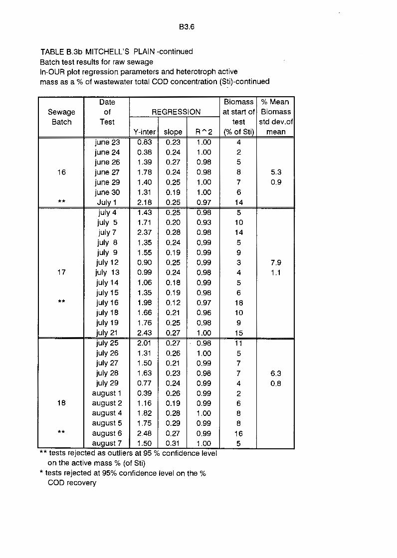
83.6
TABLE B.3b MITCHELL'S PLAIN -continued Batch test results for raw sewage In-OUR plot regression parameters and heterotroph active mass as a% of wastewater total COD concentration (Sti)-continued
Date Sewage of REGRESSION Batch Test
Y-inter slope R"'2 june 23 0.83 0.23 1.00 june 24 0.38 0.24 1.00 june 26 1.39 0.27 0.98
16 june 27 1.78 0.24 0.98 june 29 1.40 0.25 1.00 june 30 1.31 0.19 1.00
** July 1 2.18 0.25 0.97 july 4 1.43 0.25 0.98 july 5 1.71 0.20 0.93 july 7 2.37 0.28 0.98 july 8 1.35 0.24 0.99 july 9 1.55 0.19 0.99 july 12 0.90 0.25 0.99
17 july 13 0.99 0.24 0.98 july 14 1.06 0.18 0.99 july 15 1.35 0.19 0.98
** july 16 1.98 0.12 0.97 july 18 1.66 0.21 0.96 july 19 1.76 0.25 0.98 july 21 2.43 0.27 1.00 july 25 2.01 0.27 0.98 july 26 1.31 0.26 1.00 july 27 1.50 0.21 0.99 july 28 1.63 0.23 0.98 july 29 0.77 0.24 0.99
august 1 0.39 0.26 0.99 18 august 2 1.16 0.19 0.99
august 4 1.82 0.28 1.00 august 5 1.75 0.29 0.99
** august 6 2.48 0.27 0.99 august 7 1.50 0.31 1.00
** tests reJected as outliers at 95 % confidence level on the active mass% (of Sti)
* tests rejected at 95% confidence level on the % COD recovery
Biomass %Mean at start of Biomass
test std dev.of (% of Sti) mean
4 2 5 8 5.3 7 0.9 6 14 5
10 14 5 9 3 7.9 4 1.1 5 6 18 10 9 15 11 5 7 7 6.3 4 0.8 2 6 8 8
16 5

83.7
TABLE B.3b MITCHELL'S PLAIN -continued Batch test results for raw sewage In-OUR plot regression parameters and heterotroph active mass as a % of wastewater total COD concentration (Sti) -continued
Date Sewage of REGRESSION Batch Test
Y-inter slope RA2
august 13 2.6 0.27 0.96 august 15 1.69 0.24 0.98 august 16 1.15 0.27 1.00 august 18 1.31 0.26 1.00 august 19 2.08 0.22 0.99
19 august 20 2.21 0.30 0.95
* august 231 2.60 0.24 0.97
* august 23r 2.56 0.27 0.94 august 25 1.59 0.26 1.00 august 28 2.17 0.27 0.99 august 30 2.13 0.28 0.99
sept 2 2.21 0.25 0.97 sept 4 1.42 0.26 0.99 sept 6 1.21 0.25 0.99 sept 7 0.97 0.28 0.94 sept 8 1.19 0.20 0.98
20 sept 9 1.45 0.20 0.99 sept 11 1.87 0.22 0.96 sept 131 1.55 0.21 0.99 sept 13r 1.81 0.20 0.95
** sept 15 2.46 0.31 0.95 Sept 16 2.66 0.27 0.98 Sept 19 2.26 0.18 0.97 Sept 21 1.15 0.18 0.98 Sept 231 1.68 0.16 0.96
21 Sept 23r 2.34 0.26 0.99 Sept 27r 1.90 0.18 0.96 Sept 271 1.86 0.20 0.98 Sept 30r 2.06 0.21 0.98 Sept 301 1.94 0.26 0.98
** tests rejected as outliers at 95 % confidence level on the active mass % (of Sti)
* tests rejected at 95% confidence level on the % COD recovery
Biomass % Mean at start of Biomass
test std dev.of (% of Sti) mean
17 7 4 5 13 10 24 9.2 21 1.4 7 10 10 11 5 5 3 5 7.2 7 1.0
11 8 10 17 20 16 5
11 14 12.2 12 1.4 10 13 9

B3.8
TABLE B.3b MITCHELL'S PLAIN -continued Batch test results for raw sewage In-OUR plot regression parameters and heterotroph active mass as a% of wastewater total COD concentration (Sti) -continued
Date Sewage of REGRESSION Batch Test
Y-inter slope R"'2 Oct 12 1.4 0.3 1
22 Oct 13 0.62 0.29 1 Oct 17 1 .11 0.29 1 Oct 20 1.13 0.27 1
Oct 21 (3) 1.81 0.26 0.98 Oct 21 (4) 2.04 0.25 0.99 Oct 25(3) 2.11 0.31 0.97 Oct 25(4) 2.11 0.31 0.99
23 Oct 28(3) 2.14 0.3 1.00 Oct 28(4) 1.92 0.32 0.95 Nov 3(2) 0.21 0.34 1.00 Nov 3(3) 1.4 0.34 1.00 Nov 3(4) 1.49 0.32 1.00
** tests rejected as outliers at 95 % confidence level on the active mass% (of Sti)
* tests rejected at 95% confidence level on the % COD recovery
Biomass %Mean at start of Biomass
test std dev.of (% of Sti) mean
4 2 2.8 2 0.5 3 8
10 9 9 8 7.0 9 1.0 1 4 5

84.1
TABLE B.4a BORCHERDS QUARRY BATCH TEST RESULTS FOR RAW SEWAGEkinetic constants, Kmp and Uh (Id)
Sewage Date Kmp Uh of
Batch test (Id) (Id) july 12 0.96 2.64 july 19 1.20 3.12
1 july 21 1.44 3.84 july 21 2.16 4.08 july 26 0.96 5.28
* july 28 1.44 4.08 aug 6 1.92 3.36 aug 7 2.16 6.24
2 aug 9 1.68 3.60 aug 13 2.16 3.36 aug 17 2.64 5.04 aug 25 2.16 5.28 aug 26 2.40 4.80
* aug 27 2.16 4.32 3 aug 28 2.16 4.32
aug 29 2.16 5.04 aug 30 2.16 4.80 aug 31 2.40 7.20 sep 1 2.88 5.04 sep 2 2.16 4.08 sep 81 2.40 5.04 sep Br 2.16 5.28 sep 9r 2.16 6.00 sep 91 2.16 5.04
4 sep 10 2.16 5.28 sep 11 1.92 5.52 sep 12 2.16 3.84 sep 13 2.16 5.04 sept 16 1.68 4.56 sept 17 1.92 4.32 sept 18 2.16 3.36
5 sept 19 2.40 3.60 sept 21 1.92 4.08 sept 23 2.16 4.32
* tests rejected at 95% confidence level on the % COD recovery.

84.2
TABLE 8.4a BORCHERDS QUARRY BATCH TEST RESULTS FOR RAW SEWAGEkinetic constants, Kmp and Uh (Id)
Sewage Date Kmp Uh of
Batch test (Id) (Id) sept 27 1.92 5.76 sept 28 1.44 3.60 sept 29 1.44 3.12
6 sept30 1.44 3.12 oct 1 1.92 4.08 oct 2 1.68 3.60 oct 5 1.92 3.84
oct 5 u 1.92 3.36 oct 6 1.68 2.40
oct 6 u 2.16 3.12 7 oct 7 1.92 2.64
oct 7 u 2.16 2.16 oct 8 1.92 2.40 oct 9 1.68 2.16
oct 10 1.92 4.32 oct 22 2.64 2.40
oct 22 u 2.16 4.32 oct 23 1.92 1.68 oct 24 1.68 2.16
8 oct 25 1.68 2.16 oct 25 u 1.92 4.32 oct 27 1.20 1.92
oct 28 cl 1.92 3.36 oct 28 2.40 3.12 oct 28 1.92 2.40 oct 31 1.68 2.64 Nov 1 1.68 2.16 Nov2 1.92 3.12
9 Nov3 1.92 3.60 Nov4 1.92 2.64 Nov5 1.44 2.40 Nov6 1.68 2.40
* Nova 2.16 3.60 * tests rejected at 95% confidence level on the%
COD recovery.

B4.3
TABLE B.4b MITCHELL'S PLAIN BATCH TEST RESULTS FOR RAW SEWAGEkinetic constants, Kmp and Uh (Id)
Sewage Date Kmp Uh of
Batch test (Id) (Id) feb 05 3.84 4.80 feb 06 3.60 5.76 feb 07 3.84 5.52 feb 08 3.84 5.28 feb 09 3.60 5.76
10 feb 10 4.32 4.32 feb 11 3.36 3.60 feb 12 2.88 4.80 feb 13 2.88 3.60 feb 17 3.84 5.76 feb 18 3.84 4.56 feb 19 3.36 4.08 feb 20 3.84 4.08 feb 21 4.08 4.08
11 feb 22 4.08 4.80 feb 23 4.32 5.28
* feb 28 4.08 3.36 mar 1 5.28 5.04
* mar 18 2.40 3.60 mar 19 2.16 4.32 mar 20 1.92 3.84
12 mar22 3.36 3.84 mar23 2.16 3.60 mar24 2.16 3.36
* mar 26 2.40 2.40
* mar28 2.16 3.60 * tests rejected at 95% confidence level on the %
COD recovery.

84.4
TABLE B.4b MITCHELL'S PLAIN BATCH TEST RESULTS FOR RAW SEWAGEkinetic constants, Kmp and Uh (Id)
Sewage Date Kmp Uh of
Batch test (Id) (Id) april 1 2.16 4.08 april 2 1.92 3.36 april 3 1.44 2.40 april 4 2.16 4.56 april 5 1.92 4.08
13 april 6 1.68 2.88 april 7 1.68 2.64 april 8 2.16 5.52 april 9 2.16 5.76
april 10 1.44 3.36 april 11 1.44 2.16 april 13 1.92 3.60 april 19 2.16 3.36 april 20 1.92 3.60 april 21 1.68 2.88 april 22 2.40 6.48
14 april 24 1.92 3.36
* april 28 2.16 4.32 april 29 2.16 4.08 Mayos 2.16 5.04 May09 2.16 5.04 May 12 2.40 6.96 May 13 2.16 3.36 May 19 2.16 6.24 May20 2.16 4.80 May 21 2.64 3.84 May22 2.64 4.80 May23 2.64 4.56
15 May24 2.64 4.56 May27 2.40 3.36 May30 2.64 3.60
* tests rejected at 95% confidence level on the % COD recovery.

84.5
TABLE 8.4b MITCHELL'S PLAIN BATCH TEST RESULTS FOR RAW SEWAGEkinetic constants, Kmp and Uh (Id)
Sewage Date Kmp Uh of
Batch test (Id) (Id) june 23 1.92 4.32 june 24 1.92 4.56 june 26 1.92 5.28 june 27 1.92 4.56 june 29 2.16 4.56
16 june 30 1.92 3.36 July 1 2.64 4.08 july 4 1.92 4.80 july 5 2.40 3.12 july 7 2.16 5.04 july 8 1.68 4.56 july 9 1.68 3.60 july 12 1.92 4.56
17 july 13 1.92 4.56 july 14 1.68 3.12 july 15 1.92 3.36
july 16 1.20 2.40 july 18 1.44 4.08 july 19 1.68 4.80 july 21 2.16 5.04 july 25 2.16 5.04 july 26 2.40 4.56 july 27 1.92 3.84 july 28 1.92 4.32 july 29 2.40 4.08
august 1 1.92 4.80 18 august 2 1.68 3.60
august 4 2.16 5.04 august 5 2.40 5.04 august 6 2.16 5.04 august 7 3.84 4.08
* tests rejected at 95% confidence level on the% COD recovery.
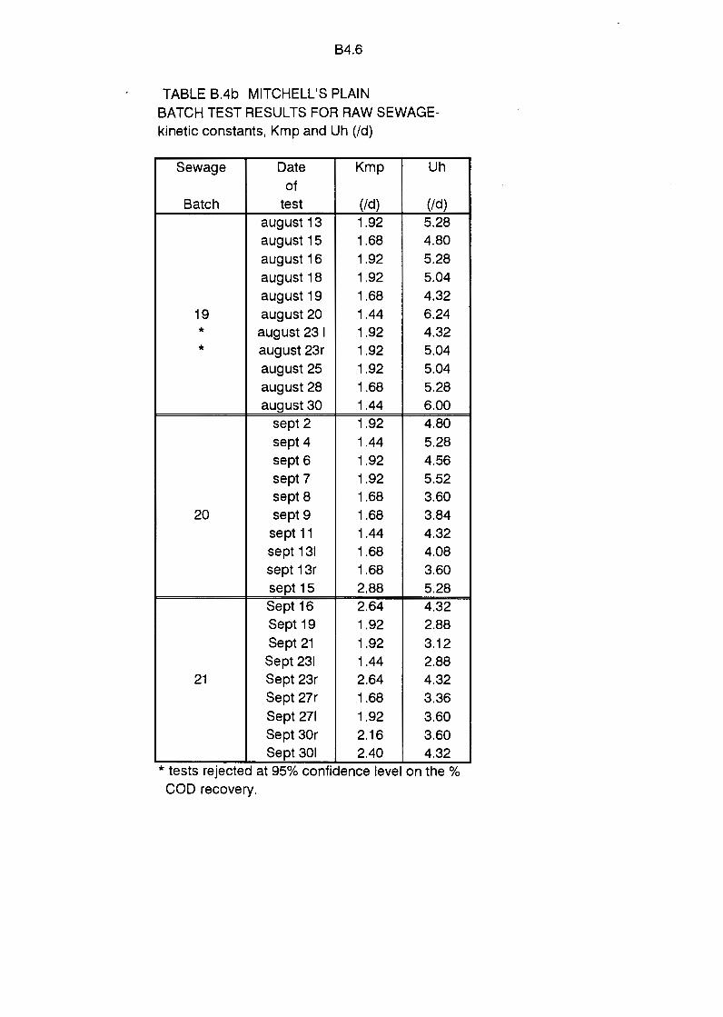
B4.6
TABLE B.4b MITCHELL'S PLAIN BATCH TEST RESULTS FOR RAW SEWAGEkinetic constants, Kmp and Uh (Id)
Sewage Date Kmp Uh of
Batch test (Id) (Id) august 13 1.92 5.28 august 15 1.68 4.80 august 16 1.92 5.28 august 18 1.92 5.04 august 19 1.68 4.32
19 august 20 1.44 6.24
* august 231 1.92 4.32
* august 23r 1.92 5.04 august 25 1.92 5.04 august 28 1.68 5.28 august 30 1.44 6.00
sept 2 1.92 4.80 sept 4 1.44 5.28 sept 6 1.92 4.56 sept 7 1.92 5.52 sept 8 1.68 3.60
20 sept 9 1.68 3.84 sept 11 1.44 4.32 sept 131 1.68 4.08 sept 13r 1.68 3.60 sept 15 2.88 5.28 Sept 16 2.64 4.32 Sept 19 1.92 2.88 Sept 21 1.92 3.12 Sept 231 1.44 2.88
21 Sept 23r 2.64 4.32 Sept 27r 1.68 3.36 Sept 271 1.92 3.60 Sept 30r 2.16 3.60 Sept 301 2.40 4.32
* tests rejected at 95% confidence level on the % COD recovery.

64.7
TABLE B.4b MITCHELL'S PLAIN BATCH TEST RESULTS FOR RAW SEWAGEkinetic constants, Kmp and Uh (Id)
Sewage Date Kmp Uh of
Batch test (Id) (Id) Oct 12 3.12 4.56
22 Oct 13 3.36 4.32 Oct 17 3.60 4.08 Oct 20 2.88 4.08
Oct 21 (3) 3.36 3.60 Oct 21 (4) 2.88 3.84 Oct 25(3) 3.36 4.80
23 Oct 25(4) 3.36 4.56 Oct 28(3) 3.36 4.80 Oct 28(4) 3.36 5.28 Nov 3(2) 2.16 5.76 Nov 3(3) 3.36 5.28 Nov 3(4) 3.36 5.28
* tests rejected at 95% confidence level on the% COD recovery.

B5.1
TABLE B.5a BOUCHERDS QUARRY BATCH TEST RESULTS FOR RAW SEWAGERBCOD % of total COD (Sti) Concentration.
Sewage Date Start RBCOD RBCOD of Total COD Cone.
Batch test (mgCOD/1) mgCOD/1 july 12 1420 254 july 19 1311 222
1 july 21 1278 232 july 21 1249 264 july 26 907 254
* july 28 855 257 aug 6 1214 143 aug 7 1427 131
2 aug 9 1322 166 aug 13 1278 133 aug 17 1246 155 aug 25 1406 193 aug 26 1406 194
* aug 27 1139 194 aug 28 1267 179
3 aug 29 1205 192 aug 30 1213 124 aug 31 1071 194 sept 1 1071 177 sept 2 1318 169 sep 81 869 181 sep Br 861 200 sep 9r 475 87 sep 91 489 89
4 sep 10 497 92 sep 11 489 105 sep 12 476 83 sep 13 436 103 sept 16 546 131 sept 17 582 128 sept 18 595 107
5 sept 19 551 104 sept 21 571 115 sept 23 551 123
** tests rejected as outliers at 95 % confidence level on% RBCOD (of Sti).
* tests rejected at 95 % confidence level on the % COD recovery.
(% of Sti) 18 17 18 21 28 30 12 9
13 10 12 14 14 17 14 16 10 18 17 13 21 23 18 18 19 21 17 24 24 22 18 19 20 22

85.2
TABLE B.5a BOUCHERDS QUARRY -continued BATCH TEST RESULTS FOR RAW SEWAGERBCOD % of total COD (Sti) Concentration.
Sewage Date Start RBCOD RBCOD of Total COD Cone.
Batch test (mgCOD/1) mgCOD/1 sept 27 638 148 sept 28 533 122 sept 29 555 123
6 sept 30 559 123 oct 1 518 126 oct 2 535 127 oct 5 627 100
oct 5u 526 92 oct 6 627 99
oct 6u 553 111 7 oct 7 607 91
oct 7u 552 127 oct 8 605 94 oct 9 542 108
oct 10 536 123 oct 22 515 93
oct 22u 593 95 oct 23 492 74 oct 24 504 80
8 oct 25 475 51 oct 25u 965 216 oct 27 564 94 oct 28 661 139 oct 28 580 132 oct 28 580 147 oct 31 590 118 Nov 1 521 97 Nov2 593 101
9 Nov3 593 83 Nov4 577 98 Nov5 512 87 Nov6 549 77
* Nova 557 106 ** tests rejected as outliers at 95 % confidence level
on% RBCOD (of Sti). * tests rejected at 95 % confidence level on the%
COD recovery.
(%of Sti) 23 23 22 22 24 24 16 17 16 20 15 23 16 20 23 18 16 15 16 11 22 17 21 23 25 20 19 17 14 17 17 14 19

B5.3
TABLE B.5b MITCHELL'S PLAIN BATCH TEST RESULTS FOR RAW SEWAGERBCOD % of total COD (Sti) Concentration.
Sewage Date Total RBCOD of COD Cone.
Batch test (mgCOD/1) (mgCOD/1 feb 05 456 73 feb 06 456 72 feb 07 456 96 feb 08 460 74
10 feb 09 520 94 feb 10 524 68 feb 11 484 75 feb 12 540 131 feb 13 544 71 feb 17 555 91 feb 18 555 90 feb 19 534 96 feb 20 551 99 feb 21 595 95
11 feb 22 551 88 feb 23 526 111
* feb 28 617 70
** mar 1 539 50
* mar 18 459 101 mar 19 455 90 mar20 480 101 mar22 512 82
12 mar 23 585 129 mar24 514 93
* mar26 514 62
* mar 28 588 82
RBCOD % of Sti
COD 16 16 21 16 18 13 15 24 13 16 16 18 18 16 16 21 11 9
22 20 21 16 22 18 12 14
** tests reJected as outliers at 95 % confidence level on% RBCOD (of Sti).
* tests rejected at 95 % confidence level on the % COD recovery.

85.4
TABLE 8.5b MITCHELL'S PLAIN -continued BATCH TEST RESULTS FOR RAW SEWAGERBCOD % of total COD (Sti) Concentration.
Sewage Date Total RBCOD of COD Cone.
Batch test (mg COD/I) (mgCOD/1 april 1 570 131 april 2 524 116 april 3 524 127 april 4 581 154 april 5 506 130
13 april 6 545 109 april 7 502 146
** april 8 518 189
** april 9 554 196 april 10 603 148 april 11 574 149 april 13 554 137 april 19 685 137 april 20 587 88 april 21 664 106 april 22 607 97
14 april 24 624 125
* april 28 504 131 april 29 645 110 May07 560 123 Mayos 548 110 May 11 552 127 May 12 605 111
RBCOD % of Sti
COD 23 22 24 26 26 20 29 36 35 25 26 25 20 15 16 16 20 26 17 22 20 23 18
** tests rejected as outliers at 95 % confidence level on% RBCOD (of Sti).
* tests rejected at 95 % confidence level on the % COD recovery.

85.5
TABLE 8.5b MITCHELL'S PLAIN -continued BATCH TEST RESULTS FOR RAW SEWAGERBCOD % of total COD (Sti) Concentration.
Sewage Date Total RBCOD of COD Cone.
Batch test (mgCOD/1) (mgCOD/1 May 19 432 94 May20 400 76 May 21 541 90 May22 521 108 May23 586 121
15 May24 472 104 May27 612 86 May30 525 95 june 23 461 101 june 24 469 70 june 26 497 139
16 june 27 533 139 june 29 405 100 june 30 545 125 July 1 464 74 july 4 556 135 july 5 504 137
** july 7 492 171 july 8 556 147 july 9 504 158
july 12 530 143 17 july 13 514 155
july 14 534 144 july 15 567 158 july 16 551 151
RBCOD % of Sti
COD 22 19 17 21 21 22 14 18 22 15 28 26 25 23 16 24 27 35 26 31 27 30 27 28 27
** tests rejected as outliers at 95 % confidence level on% RBCOD (of Sti).
* tests rejected at 95 % confidence level on the% COD recovery.

85.6
TABLE 8.5b MITCHELL'S PLAIN -continued BATCH TEST RESULTS FOR RAW SEWAGERBCOD % of total COD (Sti) Concentration.
Sewage Date Total RBCOD of COD Cone.
Batch test (mgCOD/1) (mgCOD/1 17 cont. july 19 486 126
** july 21 518 231 july 25 469 126 july 26 481 144 july 27 545 159 july 28 555 161 july 29 451 113
august 1 437 149 18 august 2 519 107
august 4 503 138 august 5 443 120 august 6 511 96 august 7 510 90
august 13 543 130 august 15 545 120 august 16 545 114 august 18 480 115
19 august19 511 158 august 20 579 179
* august 23 420 126
* august 23 420 130 august 25 469 108 august 28 584 99 august 30 567 153
sept 2 606 139 sept 4 526 132 sept 6 520 120 sept 7 520 140 sept 8 543 87
20 sept 9 508 122 sept 11 483 106 sept 131 525 89 sept 13r 525 105 sept 15 411 87
RBCOD % of Sti
COD 26 43 27 30 29 29 25 34 21 27 27 19 18 24 22 21 24 31 31 30 31 23 17 27 23 25 23 27 16 24 22 17 20 21
** tests rejected as outliers at 95 % confidence level on% RBCOD (of Sti).
* tests rejected at 95 % confidence level on the% COD recovery.

85.7
TABLE 8.5b MITCHELL'S PLAIN -continued BATCH TEST RESULTS FOR RAW SEWAGERBCOD % of total COD (Sti) Concentration.
Sewage Date Total RBCOD of COD Cone.
Batch test (mgCOD/1) (mgCOD/1
** Sept16 484 74 Sept19 583 91 Sept 21 583 99 Sept 231 511 112
21 Sept 23r 511 107 Sept 27r 556 120 Sept 271 556 117 Sept 30r 523 107 Sept 301 523 97 Oct 12 667 137
22 Oct 13 664 123 Oct 17 663 130 Oct 20 628 120
Oct 21 (3) 561 90 Oct 21 (4) 561 90 Oct 25(3) 561 76 Oct 25(4) 561 93
** Oct 28(3) 506 47 23 Oct 28(4) 506 90
Nov 3(2) 539 101 Nov 3(3) 539 121 Nov 3(4) 539 136
RBCOD % of Sti
COD 15 16 17 22 21 22 21 20 19 21 19 20 19 16 16 14 17 9
18 19 22 25
** tests rejected as outliers at 95 % confidence level on% RBCOD (of Sti).
* tests rejected at 95 % confidence level on the % COD recovery.

APPENDIX C
CONSTRUCTION AND INTERPRETATION OF STATISTICAL PWTS FOR DATA ANALYSIS
TABLE OF CONTENTS
C.1 INTRODUCTION C.2 CONSTRUCTION OF STATISTICAL PLOT C.3 INTERPRETATION OF STATISTICAL PWT C.4 TEST FOR STATISTICAL SIGNIFICANCE OF THE DIFFERENCES
BETWEEN TWO MEAN VALVES C.5 ILLUSTRATION BY AN EXAMPLE
Fig C.1: Example of a statistical probability plot for a number of RBCOD (% of total COD, Sti) derived from the batch test.
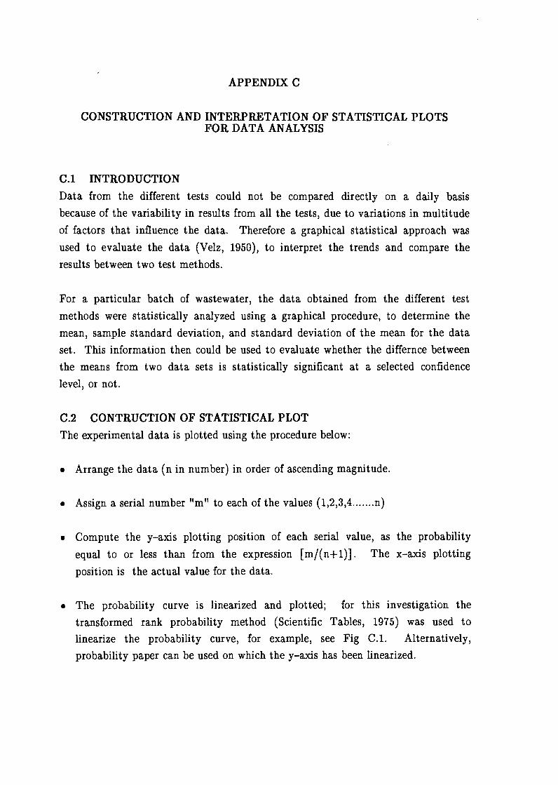
APPENDIX C
CONSTRUCTION AND INTERPRETATION OF STATISTICAL PLOTS FOR DATA ANALYSIS
C.l INTRODUCTION
Data from the different tests could not be compared directly on a daily basis
because of the variability in results from all the tests, due to variations in multitude
of factors that influence the data. Therefore a graphical statistical approach was
used to evaluate the data (Velz, 1950), to interpret the trends and compare the
results between two test methods.
For a particular batch of wastewater, the data obtained from the different test
methods were statistically analyzed using a graphical procedure, to determine the
mean, sample standard deviation, and standard deviation of the mean for the data
set. This information then could be used to evaluate whether the differnce between
the means from two data sets is statistically significant at a selected confidence
level, or not.
C.2 CONTRUCTION OF STATISTICAL PLOT
The experimental data is plotted using the procedure below:
• Arrange the data (n in number) in order of ascending magnitude.
• Assign a serial number "m" to each of the values (1,2,3,4 ....... n)
• Compute the y-axis plotting position of each serial value, as the probability
equal to or less than from the expression [m/(n+l)]. The x-axis plotting
position is the actual value for the data.
• The probability curve is linearized and plotted; for this investigation the
transformed rank probability method (Scientific Tables, 1975) was used to
linearize the probability curve, for example, see Fig C.l. Alternatively,
probability paper can be used on which the y-axis has been linearized.

C.2
C.3 INTERPRETATION OF THE STATISTICAL PLOT
The plotted data can give an indication of whether the data is normally distributed
or not:
• If a straight line can be fitted to the plot it indicates that the data have a
normal distribution.
• If a straight line can not be fitted to the plot, the data are not normally
distributed.
If the data are normally distributed it indicates that a multitude of factors have
each had an independent small influence on the measurements; if the data are not
normally distributed it indicates that one factor has had a dominating influence.
From the above, provided a straight line can be fitted to the distribution (i.e. the
data are normally distributed), it is possible to determine graphically (refer Fig C.1)
• The mean of the data plotted - this is determined as the x value where the
straight line of the distribution intercepts a vertical line extended from y = 5.
• The standard deviation of the sample, which provides a measure of the variation
of the data - this is the difference between the mean (i.e. value of x that gives
y = 5) and the value of x that gives y = 4 (or y = 6).
C.4 TEST FOR STATISTICAL SIGNIFICANCE OF THE DIFFERENCES BETWEEN TWO MEAN VALUES
Visual comparison of two data ( or data sets) is a common method of appraisal, to
determine whether they differ. However, observed differences or similarities may
not be significant as these may arise solely by chance. Statistics defines the
expected variations due to chance, to determine whether the observed differences
between two data have arisen by chance alone or are significant. In the graphical
method, by plotting of two or more series of data on the same probability plot, a
quick visual appraisal of similarities and differences can be obtained. To test
whether the visual differences in the two series of data are statistically significant, a
mathematical significant test is done as follows:
• Plot the two or more distributions to test for normality as described above.

C.3
• If normal, obtain the mean (m) and the sample standard deviation ( a) of each
series.
• Compute the standard deviation of each mean:
SD(mean) = ( a/,/ n)
where n = number of data points.
• Compute the standard deviation of the difference between the two means:
SD(difference) = ,/ { (SDmean1)2 + (SDmean2)2}
• Compute the absolute value (i.e. positive) of difference between the two means:
mean (difference) = I mean 1 - mean 2 I
• Decide upon a confidence level for the test for significance, 95% certainty or 99%
or any other level desired.
• Apply the test for statistical significance of the difference.
For example, if 95% is selected as the confidence level, subtract from the difference
between the two means [ mean( difference)], twice the standard deviation of the
difference between the two means [SD( difference)], i.e. [ mean( difference) -
2 · SD( difference)] - if a positive number is obtained it can be concluded that the
difference between the two means is statistically significant at the selected level of
confidence; if a negative value occurs, then the difference between the two means
was by chance alone, and it can be concluded that the apparent difference between
the two means is NOT statistically significant.
C.5 ILLUSTRATION BY AN EXAMPLE
An example plot is given in Fig C. l.
The mean of a set of values from an experiment is read off from the statistical graph
as the value of x that gives y = 5, i.e. in this case:

C.4
from the graph the mean = 18%
The standard deviation of a set of values is calculated from the difference between
the x value that gives y = 5 and the x value that gives y = 6, OR, from the
difference between the x value that gives y = 5 and the x value that gives y = 4, as
shown in Fig C.l, i.e. from the graph
the x value at y = 6 = 22,6
the x value at y = 4 = 13,4
the standard deviation therefore is either (22,6-18) or (18-13,4) = 4,6
The standard deviation of the mean is the standard deviation divided by the square
root of the number of values in the data set. In this case:-
number of data in the set = 12
the SDmean = 4,6/./ (12) = 1,33.
Say a second set of 10 data is analyzed as above to give:
mean= 16%
standard deviation = 5,1 %
Standard deviation of the mean is calculated:
SDmean = 5,1/./(10) = 1,61
Now, comparing the data from the two ssets:
SD( difference) = ./{(SDmean1)2 + (SDmean2)2}
= ./{1,332 + 1,612}
= 2,09
mean( difference) = I 18 - 16 I = 2%
Selecting the confidence level at 95%:
test = mean( difference) - 2 · SD( difference)
= 2 - 2·2,09
= -2,18
Since the resultant value is negative, it can be concluded that the two means are not
significantly different at the 95% confidence level.

C.5
7 I I
• ~ • Actual Results 6.5
I-
_,__ / V
co 6 0 a: a.. ~ 5.5 <( a: Cl 5 w :: a: 0 4.5 u.. Cl)
z <( 4 a: 1-
3.5
-True Normal Distr. / •
V
• /.
• /v
V ,
V mean of data =
/ (x@ y=5)
/l I
or std dev. = std dev. =
/ (x@ y=5) - (x@ y=4) (x@ y=6) - (x@ y=5)
•
Fi,: C.1:
3 10
~, , , ,, 12 14 16 18 20 22 24 26 28
RBCOD {o/o of Sti): Batch Test
Example of a statistical probability plot for a number of RBCOD (% of total COD, Sti) derived from the batch test.

APPENDIX D
COMPLETELY AEROBIC ACTIVATED SLUDGE SYSTEM
TABLE OF CONTENTS
D.1 SYSTEM LAYOUT D.2 WASTEWATER COLLECTION AND STORAGE D.3 FEED PREPARATION D.4 SYSTEM FEEDING D.5 SYSTEM MAINENANCE AND OPERATION D.6 SAMPLING AND MEASUREMENTS D.7 RESULTS
Fig D.1: Comfiguration and operation of the aerobic activated sludge system used for the conventional method to determine unbiodegradable soluble and particulate COD fractions.
Table D.la: Aerobic unit TKN and COD results. Table D.lb: Aerobic unit MLVSS, OUR, nitrates and nitrogen and COD balances. Table D.2: Mean values of the parameters measured for the aerobic unit, TKN (inf. &
eff.), COD (inf. & eff.), nitrates, OUR and MLVSS.

APPENDIX D
COMPLETELY AEROBIC ACTIVATED SLUDGE SYSTEM
D.l SYSTEM LAYOUT
The physical construction of the system was as described in detail by Burke et al.
{1986) and Clayton et al. (1989). The layout of the system consisted of a biological
reactor and secondary settling tank in series, with a recycle from the settling tank to
the biological reactor of 1:1 with respect to influent flow, see Fig D.l. The contents
of the biological reactor were completely mixed by means of independent stirring,
and aerated by passing low pressure air through a porous stone. The secondary tank
settling was an inclined tube at 60° to the horizontal and fitted with an intermittent
slow stirring (1,33 rpm) wiper blade (for details see Burke et al., 1986). Operational
details for the system are shown in Fig D.l.
D.2 WASTEWATER COLLECTION AND STORAGE
The influent for the activated sludge system was raw (unsettled) wastewater from
Borcherds Quarry and Mitchell's Plain Treatment Works in Cape Town. These
wastewaters are primarily domestic, with a very small industrial component. The
sewage was collected from the head of the works, after the screens but before the
primary sedimentation tanks. The sewage was stored at 4° C in stainless steel tanks
in a cold room at the laboratory for 10 to 14 days, then discarded and a new batch
of sewage collected; experience has shown that storage of sewage for periods longer
than about 3 weeks leads to hydrogen sulphide build-up in the tanks and a change
in the characteristics of the sewage. Immediately after storage in the cold room a
COD test was done on every batch of sewage ( COD ranged from 900 to 1 400
mgCOD/l).
D.3 FEED PREPARATION
The total COD concentration for the four test methods (i.e. square wave, batch test,
flocculation-filtration test and the aerobic unit) was set at 500±50 mg COD/ t. Knowing the total COD concentration of the sewage batch collected, volumes of
wastewater and tap water required to dilute the wastewater to the required
concentration could be calculated. The contents of the storage tank were
thoroughly mixed and the calculated volume of wastewater was then drawn from the
storage tank daily: The wastewater was drawn from a tap at the bottom of the
tank, passed through a sieve (1mm) into a graduated 20l plastic bucket. Then the

D.2
calculated volume of tap water was added to dilute the wastewater to the COD
concentration required for the tests. To increase the alkalinity of the influent (to
maintain the pH in the reactor at :1:7,5), 1 or 2 te~spoons of sodium bicarbonate
were added to the diluted wastewater. After thorough mixing, a sample was drawn
for influent analysis.
D.4 SYSTEM FEEDING
From the diluted wastewater above, daily the feed (10£.) for the activated sludge
system was drawn and stored in an upright PVC bucket which had a stirrer driven
by a motor at 10 rpm, to keep the contents in the bucket completely mixed and
discourage settling of the solid particles in the bucket. The surface of the bucket
was covered by a floating plastic disc to discourage entrainment of air from the
atmosphere into the feed. The bucket was placed in a large chest refrigerator at a
temperature of 4-8° C to minimize biological degradation of the sewage. The
wastewater was pumped at a constant rate from the storage bucket to the activated
sludge system over the 24 h period. The feed bucket was cleaned daily with boiling
water.
D.5 SYSTEM MAINTENANCE AND OPERATION
The general maintenance and operational procedures set out in detail by Burke et al.
(1986) and Clayton et al. (1989) were followed.
The volume of the mixed liquor in the system was maintained at 10£., by controlling
the level in the reactor. The sludge age was controlled hydraulically (WRC, 1984)
at 12 d, by wasting daily from the reactor 0,83£. of the mixed liquor (including any
samples drawn for analysis). The system was operated in a temperature controlled
room, kept constant at 20° C. In the biological reactor, pH was controlled at 7,5
(±0,2) and oxygen concentration at 4 mgO/l (except during OUR tests).
D.6 SAMPLING AND MEASUREMENTS
From the unit the following parameters were measured on a daily basis:
• the feed total COD concentration (Standard Methods, 1985)
• the effluent COD concentration, filtered and unfiltered (Standard Methods, 1985)

D.3
• the influent and effluent TKN concentrations , unfiltered and filtered (Standard
Methods, 1985)
• the effluent nitrate concentration (Technicon Auto Analyzer)
• the reactor mixed liquor suspended solids (MLSS) and mixed liquor volatile
suspended solids (MLVSS) concentrations (Standard Methods, 1985)
• the oxygen utilization rate (OUR) in the reactor.
The OUR in the reactor was measured by immersing in the mixed liquor a DO
probe (YSI) connected to a DO meter which was then connected to a Hewlett
Packard chart recorder (Model 17500 A). The OUR was measured by raising the
DO in the mixed liquor from 4,0 to 6,0 mgO/t (by opening an air valve on the
tubing from the pump) then switching off the air. The decrease in the DO
concentration with time was recorded. From the slope of the DO concentration
time line, the OUR was calculated (mgO/t/h). After about 5 minutes the air was
switched back on and the mixed liquor DO maintained at 4,0 mgO/t. The OUR
readings were taken twice a day and an average calculated for the day.
D.7 RESULTS
Daily results for the activated sludge system are listed in Tables D.la and b. For
each wastewater batch tested, the daily results were averaged, and the averages are
listed in Table D.2. From the averaged data, for each wastewater batch COD and
nitrogen balances were calculated using the procedures set out by Ekama et al. (1986) and these are also listed in Table D.2. Acceptability of the data is based on
the mass balances being within the range of 90-110%. From Table D.2, with the
exception of sewage batch No.21 all the nitrogen mass balances fell within this
acceptable range; sewage batch No.21 was rejected for analysis. However, the COD
mass balances all were too high (average mass balance 119%). The high COD mass
balances were unexpected; usually-for completely aerobic systems acceptable COD
mass balances can be obtained without undue difficulty. A number of parallel
completely aerobic units operated in the UCT laboratory by undergraduate research
students gave very similar COD mass balances (Ubisi, 1994; Jadav, 1994; Hercules,
1994). Attempts to trace the errors in the measurements contributing to the COD
mass balance indicated a problem in measurement of the OUR; however, this
problem could not be resolved successfully. Since the problem in the COD mass

D.4
balance was located in measurement of the OUR, the OUR parameter could not be
used to determine the unbiodegradable particulate fraction of the influent COD
(fup) (Ekama et al., 1986). Instead, the measured MLVSS concentration was used
to determine fup using Eq (9.1); the error in the OUR measurement will not affect
the estimate for fup using this method. Accordingly, from the averaged data fus was
calculated as the effluent COD concentration divided by the influent COD
concentration, see Table D.2 ( daily fus values were also calculated for comparison
with batch test results in Chapter 7 and are listed in Appendix G). From the
averaged data and with fus calculated, fup was calculated using Eq (9.1) - these
values were used for comparison with batch test data, see Chapter 9.

Infl
uen
t
Qi=
101
/d
Fiv;
D.1
:
Aer
ob
ic
reac
tor
VP =
101
Was
te
Slu
dg
e R
s=
12
d
Sec
on
dar
y se
ttli
ng
ta
nk
Eff
luen
t
Slu
dg
e re
cycl
e
1:1
Con
figu
rati
on a
nd o
pera
tion
of
the
aero
bic
acti
vate
d sl
udge
sys
tem
use
d fo
r th
e co
nven
tion
al m
etho
d to
det
erm
ine
unbi
odeg
rada
ble
solu
ble
and
part
icul
ate
CO
D f
ract
ions
(E
kam
a et
al.,
198
6).
~
C11

D.6
TABLE D.1A-AEROBIC UNIT TKN and COD RESULTS. Qw 0.833 litres/da fcv 1.48 mgCOD/mgVSS
Qi 10 litres/da f 0.2 mgVSS/mgVSS
Vp 10 litres bh 0.24 /day IXB 0.1 mgN/mg yh 0.45 mgVSS/mgCOD
Sewage Dates of TKN ( mg N/1) COD (mgCOD/1) fus
Batch tests influent effluent influent effluent May20 56 1 396* 53 0.13 May21 59 5 541 49 0.09
May22 77 6 521 49 0.09 May23 76 6 586 49 0.08
15 May24 78 3 468 47 0.10 May25 85 10 456 57 0.13
May26 85 9 603 53 0.09 May27 81 6 534 47 0.09 May28 82 6 538 39 0.07 May29 80 6 531 39 0.07 May30 70 5 525 47 0.09 May31 80 5 538 49 0.09 June 1 80 5 534 41 0.08 June 2 79 4 529 38 0.07 June 3 81 5 501 30 0.06 June 4 76 5 517 40 0.08
15 a June 5 73 4 528 48 0.09 June 6 78 4 508 40 0.08 June 7 81 8 492 36 0.07 June 8 79 14 500 58 0.12 June 9 75 13 464 54 0.12
June 10 69 12 367* 48 0.08 June 11 71 10 548 52 0.10 June 12 65 7 460 42 0.09 June 13 75 8 496 44 0.09
16 June 14 76 10 500 48 0.10 June 15 75 5 444 42 0.10 June 16 76 9 476 56 0.12 June 17 69 11 508 71 0.14 June 18 69 6 512 40 0.08 June 19 68 8 468 40 0.09

D.7
TABLE D.1A-continued
AEROBIC UNIT TKN and COD RESULTS. Qw 0.833 litres/da fcv 1.48 mgCOD/mgVSS Qi 10 litres/da f 0.2 mgVSS/mgVSS Vp 10 litres bh 0.24 /day IXB 0.1 mgN/mg yh 0.45 mgVSS/mgCOD
Sewage Dates of TKN ( mg N/1) COD (mgCOD/1) fus Batch tests influent effluent influent effluent
June 20 68 7 493 40 0.08 June 21 69 12 493 40 0.08 June 22 69 10 433 52 0.12 June 23 68 9 493 42 0.09 June 24 70 6 461 52 0.11
16 June 25 74 6 497 50 0.10 cont. June 26 69 7 497 30 0.06
June 27 69 6 533 52 0.10 June 28 67 5 465 40 0.09 June 29 69 7 453 40 0.09 June 30 76 6 545 69 0.13 July 1 67 7 461 48 0.10 July 2 55 6 569 36 0.06 July 3 56 6 508 28 0.06 July 4 59 11 516 34 0.07 July 5 53 12 504 52 0.10
17 July 6 56 7 516 48 0.09 July 7 62 6 492 56 0.11 July 8 57 6 556 48 0.09 July 9 57 5 504 36 0.07 July 10 57 4 508 34 0.07 July 11 57 4 555 47 0.08 July 12 55 6 530 57 0.11 July 13 60 5 514 36 0.07 July 14 57 7 534 36 0.07 July 15 57 5 567 45 0.08 July 16 59 4 551 36 0.07 July 17 59 4 506 49 0.10 July 18 58 5 470 33 0.07 July 19 56 5 518 41 0.08 July 20 58 5 486 37 0.08 July 21 57 5 519 34 0.07

D.8
TABLE D .1 A-continued AEROBIC UNIT TKN and COD RESULTS. Qw 0.833 litres/da fcv 1.48 mgCOD/mgVSS
Qi 10 litres/da f 0.2 mgVSS/mgVSS
Vp 10 litres bh 0.24 /day IXB 0.1 mgN/mg yh 0.45 mgVSS/mgCOD
Sewage Dates of TKN ( mg N/1) COD (mgCOD/1) fus
Batch tests influent effluent influent effluent
July 22 55 4 481 49 0.10 July 23 49 5 543 61 0.11
July 24 55 5 486 75 0.16 July 25 53 3 469 37 0.08 July 26 54 3 481 39 0.08 July 27 56 4 545 41 0.08 July 28 55 3 555 37 0.07 July 29 53 4 451 49 0.11 July 30 54 4 464 43 0.09
18 July 31 55 3 484 39 0.08 August 1 53 5 437 33 0.08 August 2 55 4 519 33 0.06 August 3 55 4 488 72 0.15 August 4 57 2 503 41 0.08 August 5 51 4 443 24 0.06 August 6 56 4 511 28 0.06 August 7 58 2 510 33 0.06 August 8 53 4 532 35 0.06 August 9 52 3 514 35 0.07
August 10 52 5 524 47 0.09 August 11 59 6 534 43 0.08 August 12 57 3 510 26 0.05 August 13 60 2 543 24 0.04
19 August 14 60 3 567 41 0.07 August15 60 6 545 55 0.10 August 16 60 4 480 57 0.12 August 17 60 6 500 45 0.09 August 18 57 5 480 45 0.09

D.9
TABLE D.1A-continued AEROBIC UNIT TKN and COD RESULTS. Qw 0.833 litres/da fcv 1.48 mgCOD/mgVSS Qi 10 litres/da f 0.2 mgVSS/mgVSS Vp 10 litres bh 0.24 /day IXB 0.1 mgN/mg yh 0.45 mgVSS/mgCOD
Sewage Dates of TKN ( mg N/1) COD (mgCOD/1) fus Batch tests influent effluent influent effluent
August 19 58 4 511 24 0.05 August 20 57 3 579 49 0.08 August 21 59 5 455 36 0.08 August 22 55 3 524 20 0.04 August 23 56 5 420 24 0.06
19 August 24 50 6 482 31 0.06 cont. August 25 52 5 469 28 0.06
August 26 56 6 485 20 0.04 August 27 57 6 524 25 0.05 August 28 58 6 543 23 0.04 August 29 58 6 563 27 0.05 August 30 58 6 567 45 0.08 August 31 58 6 567 45 0.08
sept 5 45 4 526 41 0.08 sept 6 44 5 520 41 0.08 sept 7 45 7 520 33 0.06 sept 8 45 5 543 41 0.08
20 sept 10 43 5 462 45 0.10 sept 11 43 5 483 45 0.09 sept 12 43 5 470 37 0.08 sept 13 44 4 448 37 0.08 sept 14 44 5 468 37 0.08 sept 15 44 5 411 26 0.06 sept 16 48 4 484 33 0.07 sept 17 45 5 623 41 0.07 sept 18 52 4 595 33 0.06
21 sept 19 53 4 583 33 0.06 sept 20 52 4 548 62 0.11 sept 21 53 6 583 51 0.09 sept 22 56 4 538 53 0.10 sept 23 56 5 570 49 0.09 sept 24 51 5 484 33 0.07

D.10
TABLE D.1 A-continued AEROBIC UNIT TKN and COD RESULTS. Qw 0.833 litres/da fcv 1.48 mgCOD/mgVSS Qi 10 litres/da f 0.2 mgVSS/mgVSS Vp 10 litres bh 0.24 /day IXB 0.1 mgN/mg yh 0.45 mgVSS/mgCOD
Sewage Dates of TKN ( mg N/1) COD (mgCOD/1) fus Batch tests influent effluent influent effluent
sept 25 54 5 579 39 0.07 21 sept 26 54 7 478 53 0.11
cont. sept 27 55 5 556 45 0.08 sept 28 54 7 523 55 0.11 sept29 54 5 566 62 0.11 sept 30 53 5 523 33 0.06 oct 13 54 5 560 36 0.06
22 oct 14 59 5 524 32 0.06 oct 15 59 5 562 40 0.07 oct 16 58 5 562 40 0.07 oct 17 58 5 562 40 0.07 oct 21 41 7 402 33 0.08 oct 22 44 6 469 31 0.07 oct 23 44 4 460 43 0.09 oct 24 48 7 452 33 0.07
23 oct 25 38 5 568 45 0.08 oct 26 51 7 560 45 0.08 oct 27 54 6 556 37 0.07 oct 28 54 6 511 33 0.06 oct29 55 5 514 45 0.09 oct 30 54 6 551 37 0.07 oct 31 52 7 530 35 0.07 nov 1 55 5 528 53 0.10 nov 2 52 5 567 55 0.10
*data ommitted from calculations due to operational problems (eg unit overflow) or transition between batches of sewage.

D.11
TABLE D.1B AEROBIC UNIT MLVSS,OUR,NITRATES and NITROGEN and COD BALANCES Qw Qi Vp IXB
Sewage Batch
15
15 a
16
0.833 litres/da 1 O litres/da 1 o litres
0.1 mgN/mg
Dates of Nitrates tests (mgN/1)
May20 40 May 21 46 May22 49 May23 54 May24 56 May25 56 May26 55 May27 57 May28 59 May29 62 May30 59 May31 53 June 1 54 June 2 59 June 3 56 June 4 59 June 5 60 June 6 60 June 7 59 June 8 66 June 9 56
June 10 47 June 11 46 June 12 46 June 13 45 June 14 48 June 15 48 June 16 46 June 17 46 June 18 46 June 19 47
fcv f
bh yh
MLVSS (mgVSS/1)
1340 1320 1274 1206 1532 1602 1550 1438 1230 1370 1478 1396 1846* 1270 1306 1284 1330 1500 1136 1346 1370 550* 842* 894* 878* 838* 908* 1006* 1232 1192 1082
1 .48 mgCOD/mgVSS 0.2 mgVSS/mgVSS
0.24 /day 0.45 mgVSS/mgCOD
OUR % Nitrogen %COD (mg0/1/hr Balance Balance
20 93 130 26 105 114 30 86 135 30 92 114 28 92 139 30 94 158 29 90 113 31 93 131 34 92 139 30 100 121 29 109 123 28 88 120 27 74 83 29 93 117 30 89 131 25 98 103 20 102 80 24 98 104 24 94 98 22 115 90 25 107 121 23 86 123 24 79 74 31 82 127 28 71 105 29 76 106 30 71 122 30 73 119 35 97 168 33 90 150 28 94 137

D.12
TABLE D.1B AEROBIC UNIT MLVSS,OUR,NITRATES and NITROGEN and COD BALANCES Qw 0.833 litres/da fcv 1.48 mgCOD/mgVSS Qi 10 litres/da f 0.2 mgVSS/mgVSS
Vp 10 litres bh 0.24 /day IXB 0.1 mgN/mg yh 0.45 mgVSS/mgCOD
Sewage Dates of Nitrates MLVSS OUR % Nitrogen %COD
Batch tests (mgN/1) (mgVSS/1) (mg0/1/hr Balance Balance June 20 45 1396 30 94 147
16 June 21 41 1654 30 97 157 June 22 41 1750 27 96 168 June 23 48 1632 25 104 126 June 24 43 1420 23 86 127 June 25 49 1296 27 88 128 June 26 49 1296 27 97 123 June 27 47 1444 25 94 117 June 28 47 1208 24 93 118 June 29 44 1306 23 90 122 June 30 47 1138 26 83 113 July 1 48 1372 24 99 125 July 2 42 1214 20 106 83 July 3 36 1394 22 95 111 July 4 31 874* 20 70 73 July 5 31 1076* 18 80 66 July 6 30 1016* 20 65 76 July 7 30 838* 20 57 82 July 8 27 914* 20 58 73
17 July 9 28 1068* 20 58 77 July 10 28 804* 20 56 76 July 11 29 824* 20 57 71 July 12 26 796* 15 59 56 July 13 29 1228* 30 56 122 July 14 29 1044* 22 63 81 July 15 35 1059* 22 71 73 July 16 34 1018* 25 65 87 July 17 31 1180* 30 59 124 July 18 30 1294 35 79 190 July 19 32 1378 27 87 137 July 20 32 1356 28 83 150 July 21 33 1286 20 86 100

D.13
TABLE D.1B AEROBIC UNIT MLVSS,OUR,NITRATES and NITROGEN and COD BALANCES Qw Qi Vp IXB
Sewage Batch
18
19
0.833 litres/da 1 O litres/da 1 o litres
0.1 mgN/mg
Dates of Nitrates tests (mgN/1)
July 22 34 July 23 32 July 24 32 July 25 29 July 26 37 July 27 38 July 28 32 July 29 33 July 30 32 July 31 32
August 1 31 August 2 36 August 3 34 August 4 36 August 5 36 August 6 33 August 7 39 August 8 36 August 9 36
August 10 34 August 11 46 August 12 46 August 13 42 August 14 49 August15 40 August 16 51 August 17 43 August 18 38
fcv f
bh yh
MLVSS (mgVSS/1)
1262 1404 1344 1284 1230 1322 1286 940* 1440 1232 1048 1314 1332 1240 1406 1100 1294 1268 1090 1368 1444 1346 1716 1592 1782 1538 1516 1496
1.48 mgCOD/mgVSS 0.2 mgVSS/mgVSS
0.24 /day 0.45 mgVSS/mgCOD
OUR % Nitrogen %COD (mg0/1/hr Balance Balance
20 88 110 27 99 136 22 87 129 21 80 121 22 93 114 23 95 108 20 84 95 20 69 84 22 90 129 20 82 108 20 84 115 26 93 125 28 89 156 25 84 125 24 100 138 24 82 116 24 88 116 24 94 114 20 93 94 22 96 112 38* 108 173 35* 106 161 36* 96 168 30 109 129 27 101 136 27 112 138 22 102 113 20 97 112

D.14
TABLE 0.1B AEROBIC UNIT MLVSS,OUR,NITRATES and NITROGEN and COD BALANCES Qw 0.833 litres/da fcv 1.48 mgCOD/mgVSS Qi 10 litres/da f 0.2 mgVSS/mgVSS
Vp 10 litres bh 0.24 /day IXB 0.1 mgN/mg yh 0.45 mgVSS/mgCOD
Sewage Dates of Nitrates MLVSS OUR % Nitrogen %COD
Batch tests (mgN/1) (mgVSS/1) (mg0/1/hr Balance Balance August 19 37 1484 25 92 125 August 20 41 1738 25 103 117 August 21 35 1366 20 86 116 August 22 37 1490 20 96 98 August 23 39 1164 22 95 124
19 August 24 37 1208 20 107 102 cont. August 25 36 1400 25 101 136
August 26 37 1330 20 97 102 August 27 39 1318 24 97 112 AUQUSt 28 43 1360 28 103 123 August 29 43 1450 25 105 109 August 30 45 1028 21 103 83 August 31 32 1206 28 82 127
sept 5 33 1406 24 108 122 sept 6 31 1286 20 106 103 sept 7 31 1068 20 104 97 sept 8 31 1204 20 103 97
sept 10 30 1002 28 100 152 20 sept 11 31 1002 27 103 140
sept 12 31 1050 14 103 77 sept 13 31 1024 20 98 112 sept 14 30 928* 26 79 112 sept 15 26 1122 24 92 151 sept 16 29 1774* 28 69 118 sept 17 28 1028 25 92 103 sept 18 30 1206 27 85 116
21 sept 19 28 1292 23 80 106 sept 20 28 1310 28 83 140 sept 21 30 1220 25 87 114 sept 22 28 1254 25 75 127 sept 23 31 1234 24 82 112 sept 24 32 1214 23 92 121

D.15
TABLED.1B AEROBIC UNIT MLVSS,OUR,NITRATES and NITROGEN and COD BALANCES Qw 0.833 litres/da fcv 1.48 mgCOD/mgVSS Qi 10 litres/da f 0.2 mgVSS/mgVSS Vp 10 litres bh 0.24 /day IXB 0.1 mgN/mg yh 0.45 mgVSS/mgCOD
Sewage Dates of Nitrates MLVSS OUR % Nitrogen %COD Batch tests (mgN/1) (mgVSS/1) (mg0/1/hr Balance Balance
sept 25 30 1232 24 84 109 21 sept 26 30 1210 24 87 134
cont. sept 27 30 1258 24 83 115 sept 28 30 1196 23 86 118 sept 29 30 1092 22 82 103 sept 30 31 1140 27 86 130 act 13 37 1352 24 99 109
22 act 14 37 1400 25 91 121 act 15 37 1392 25 91 114 act 16 36 1456 22 91 104 act 17 37 1678 25 97 120 act 21 33 1882 24 136 171 act 22 32 1768 24 120 145 act 23 32 1678 25 113 151 act 24 29 1780 25 106 159
23 act 25 32 1472 25 129 118 act 26 31 1648 25 101 126 act 27 29 1660 24 91 123 act 28 29 1668 24 91 133 act 29 29 1598 25 86 138 act 30 27 1716 25 87 132 act 31 28 1438 24 90 124 nov 1 29 1528 23 85 125 nov2 29 1460 24 89 119
*data ommitted from calculations due to operational problems (eg unit overflow) or transition between batches of sewage.

TA
BLE
D.2
M
ean
valu
es o
f th
e p
aram
eter
s m
easu
red
fro
m t
he
ae
rob
ic u
nit
i.e T
KN
(eff.
and
inf.)
,CO
D(e
ff. a
nd
inf.)
,nitr
ates
,OU
R,a
nd M
LVS
S
Sew
age
Dat
es o
f TK
N
CO
D
Nitr
ates
m
gN/1
m
gCO
D/1
ef
fluen
t b
atc
h
Tes
ts
influ
ent
efflu
ent
influ
en
t ef
fluen
t m
gN/1
15
20
-31
May
76
6
531
48
54
15a
1-9
Jun
e
78
7 51
4 43
59
16
1 O
Jun
e-1
Jul
70
8 48
7 46
46
17
2
-21
Ju
ly
57
6 52
1 41
34
18
22
Jul
y-10
Au
54
4 49
7 43
34
19
11
-31
Au
g
57
5 51
7 35
41
20
5-
15 S
ep
t 44
5
485
38
31
21
16-3
0 S
ep
t*
53
5 54
9 45
30
22
1-
12 O
ct
57
5 54
9 36
37
23
13
Oct
-2 N
ov
51
6 51
9 40
31
*r
eje
cte
d b
atc
h d
ue
to
sys
tem
op
era
tion
al p
rob
lem
s.
MLV
SS
fu
s fu
p
OU
R
mg/
I m
g0/1
/hr
1395
0.
09
0.11
29
13
18
0.08
0.
09
25
1361
0.
09
0.14
27
13
20
0.08
0.
09
23
1261
0.
09
0.09
23
14
27
0.07
0.
12
24
1129
0.
08
0.05
22
12
06
0.08
0.
03
24
1381
0.
07
0.08
25
16
27
0.08
0.
19
23
%
BA
LAN
CE
S
N
CO
D
94
126
99
104
93
134
90
115
90
120
102
116
103
116
85
115
94
116
99
125
t:i -O')

APPENDIXE
COMPREHENSIVE DATA FOR THE FLOCCULATION-FILTRATION METHOD TO DETERMINE RBCOD
TABLE OF CONTENTS
Table El.a: COD concentrations after flocculation and filtration through 0.45µm and glass fibre filters on the influent samples from Borchards Quarry.
Table El.b: COD concentrations after flocculation and filtration through 0.45µm and glass fibre filters on the influent samples from Mitchell's Plain.
Table E2.a: COD concentrations after flocculation and filtration through 0.45µm and glass fibre filters on the effluent samples from Borchards Quarry.
Table E2.b: COD concentrations after flocculation and filtration through 0.45µm and glass fibre filters on the effluent samples from Mitchell's Plain.
Table E3.a: COD concentrations after flocculation and filtration through 0.45µm and calculated RBCOD (as a % of total COD, Sti) for Borchards Quarry.
Table E3.b: COD concentrations after flocculation and filtration through 0.45µm and calculated RBCOD (as a % of total COD, Sti) for Mitchell's Plain.
Table E4.a: COD concentrations after flocculation and filtration through glass fibre (GF/C) filters and calculated RBCOD (as a % of total COD, Sti) for Borchards Quarry.
Table E4.b: COD concentrations after flocculation and filtration through glass fibre (GF/C) filters and calculated RBCOD (as a % of total COD, Sti) for Mitchell's Plain.

E1 .1
TABLE E.1a COD concentrations after flocculation and filtration through 0.45 micron and glass fibre filters papers on the INFLUENT samples from Boucherd's Quarry.
Sewage Date Total COD after floc.-filter (mgCOD/1) of COD gf/c .45 micro
Batch test (mgCOD/1 filtered filtered sept 16 546 140 140 sept 17 582 157 153 sept 18 595 161 161
5 sept 19 551 143 159 sept 21 571 158 154 sept 22 577 141 125 sept 23 551 190 173 sept 27 638 149 149 sept 28 638 169 169 sept 29 533 157 157
6 sept 30 559 173 123 oct 1 518 160 152 oct 2 535 169 164 oct 5 627 135 150 oct 6 627 131 166 oct 7 607 144 148
7 oct 8 605 174 142 oct 9 542 130 126
oct 10 536 131 131 oct 26 577 126 126 oct 27 564 122 122
8 oct 28 661 172 160 oct 29 661 141 137 oct 30 479 138 138 oct 31 590 147 147 nov 1 521 138 138 nov 2 593 145 145
9 nov 3 593 171 171 nov 4 577 165 165 nov 5 512 144 144 nov 6 549 126 126 nov 8 557 156 156

E1 .2
TABLE E.1 b COD concentrations after flocculation and filtration through 0.45 micron and glass fibre filters papers on the INFLUENT samples from Mitchell's Plain
Sewage Date Total COD after floc.-filter (mgCOD/1) of COD gf/c .45 micro
Batch test (mgCOD/1 filtered filtered jan 20 536 164 164 jan 21 557 197 161 jan 22 569 140 124 jan 23 667 173 178 jan 24 504 163 135
10a jan 25 673 123 141 jan 26 609 135 125 jan 27 593 141 131 jan 28 665 117 182 jan 31 528 131 179 feb 1 481 138 128 feb 2 476 147 136 feb 4 440 122 120 feb 5 456 98 124 feb 6 456 143 130 feb 7 456 118 109
10 feb 8 460 119 129 feb 9 520 119 120
feb 10 524 117 115 feb 11 484 156 165 feb 12 540 149 145 feb 13 544 120 119 feb 17 555 151 151 feb 18 555 159 159 feb 19 534 153 141 feb 20 551 162 150 feb 21 595 170 170
11 feb 22 551 142 146 feb 23 526 146 128 feb 24 621 132 149 feb 25 503 118 118 mar 1 539 136 136 mar2 552 134 141

E1 .3
TABLE E.1 b- continued
COD concentrations after flocculation and filtration through 0.45 micron and glass fibre filters papers on the INFLUENT samples.
Sewage Date Total COD after floc.-filter (mgCOD/1) of COD gf/c .45 micro
Batch test (mgCOD/1 filtered filtered mar 19 455 134 158 mar20 480 138 138 mar 21 480 154 154 mar22 512 110 146
12 mar23 585 150 172 mar24 512 151 151 mar25 514 129 129 mar26 514 145 143 mar27 681 153 153 mar28 588 118 118 apr1 570 175 159 apr2 524 138 138 apr3 524 154 156 apr4 581 169 163 apr5 506 154 154
13 apr6 545 150 171 apr7 502 163 161 apr8 518 171 171 apr9 554 183 171
apr10 603 161 180 apr11 574 171 171 apr19 685 192 192 apr20 587 171 162 apr 21 664 163 163 apr22 607 193 170 apr23 636 168 168 apr24 624 189 166 apr25 624 176 176 apr26 602 168 178
14 apr27 627 193 193 apr28 504 151 148 apr29 645 204 204 may9 560 168 151 may 10 548 155 155

E1 .4
TABLE E.1 b- continued COD concentrations after flocculation and filtration through 0.45 micron and glass fibre filters papers on the INFLUENT samples.
Sewage Date Total COD after floc.-filter (mgCOD/1) of COD gf/c .45 micro
Batch test (mgCOD/1 filtered filtered 14 cont. may 11 552 164 168
may 12 605 155 155 may 13 642 180 180 may 14 598 194 178 may 15 598 178 176 may 16 626 184 164 may 19 432 115 121 may20 400 103 97 may21 541 121 121 may22 521 147 143 may23 586 156 147
15 may24 472 142 147 may 25 456 145 119 may26 603 150 160 may27 612 135 135 may 28 534 113 96 may29 531 113 117 may30 525 109 109 june 1 534 103 99 jun 23 461 112 108 jun 24 469 118 122 jun 26 497 130 124 jun 27 533 134 126
16 jun 28 465 110 110 jun 29 441 116 104 jun 30 545 122 102 jul 1 464 122 102

E1 .5
TABLE E.1b-continued
COD concentrations after flocculation and filtration through 0.45 micron and glass fibre filters papers on the INFLUENT samples.
Sewage Date Total COD after floc.-filter (mgCOD/1) of COD gf/c .45 micro
Batch test (mgCOD/1 filtered filtered jul 4 556 141 133 jul 5 504 160 140 jul 6 516 135 111 jul 7 492 129 129 jul 8 556 121 141
17 jul 12 530 150 150 jul 13 514 130 125 jul 15 567 130 159 jul 16 551 154 162 jul 18 461 138 138 jul 20 477 122 122 jul 26 481 124 112 jul 27 545 135 135 jul 28 555 154 154 jul 29 451 102 122 aug 1 437 116 116
18 aug 2 519 125 134 aug 3 488 103 99 aug 4 503 147 147 aug 5 443 149 149 aug 6 511 128 128 aug 8 532 102 106
aug 15 545 139 139 aug 16 545 174 174 aug 17 480 185 185 aug 18 480 160 160
19 aug 19 511 173 173 aug 22 579 221 221

E1.6
TABLE E.1 b- continued COD concentrations after flocculation and filtration through 0.45 micron and glass fibre filters papers on the INFLUENT samples.
Sewage Date Total COD after floc.-filter (mgCOD/1) · of COD gf/c .45 micro
Batch test (mgCOD/1 filtered filtered Sept 5 484 126 126 Sept 7 520 153 171 Sept 8 543 182 182 Sept 9 508 162 158
20 Sept 11 483 140 140 Sept 12 508 130 134 Sept 13 525 113 117 Sept 14 525 145 145 Sept 15 411 127 130 Sept 19 583 135 144 Sept20 517 88 88 Sept 21 548 124 115 Sept22 517 141 139
21 Sept 23 511 118 118 Sept26 556 130 130 Sept 27 556 116 128 Sept 28 523 127 127 Sept 29 667 138 138 Sept30 523 103 103

E2.1
TABLE E.2a COD concentrations after flocculation and filtration through 0.45 micron and glass fibre filter papers on the EFFLUENT samples from an activated sludge system treating Boucherd's Quarry wastewater.
Sewage Date Total COD after floc.-filter (mgCOD/1) of COD gf/c .45 micro
Batch test (mg COD/I) filtered filtered sept 16 546 35 31 sept 17 582 39 35 sept 18 595 47 63
5 sept 19 551 61 45 sept 21 571 57 53 sept 22 577 44 60 sept 23 551 60 56 sept 27 638 56 44 sept 28 638 56 48 sept 29 533 62 60
6 sept 30 559 49 49 oct 1 518 58 58 oct 2 535 49 33 oct 5 627 41 41 oct 6 627 41 41 oct 7 607 39 37
7 oct 8 605 53 53 oct 9 542 33 49
oct 10 536 47 47 oct 26 577 57 57 oct 27 564 55 59
8 oct 28 661 67 67 oct 29 661 45 45 oct 30 479 57 57 oct 31 590 45 45 nov 1 521 41 37 nov 2 593 45 45 nov3 593 49 45
9 nov4 577 30 30 nov 5 512 55 51 nov 6 549 63 59 nov 8 557 49 45

E2.2
TABLE E.2b COD concentrations after flocculation and filtration through 0.45 micron and glass fibre filter papers on the EFFLUENT samples from an activated sludge system treating Mitchell's Plain wastewater.
Sewage Date Total COD after floc.-filter (mgCOD/1) of COD gf/c .45 micro
Batch test (mgCOD/1) filtered filtered jan 20 536 40 40 jan 21 557 47 47 jan 22 569 55 51 jan 23 667 77 58 jan 24 504 66 34
10a jan 25 673 22 22 jan 26 609 40 40 jan 27 593 36 40 jan 28 665 44 42 jan 31 528 65 63 feb 1 481 41 41 feb 2 476 47 25 feb 4 440 29 29 feb 5 456 41 37 feb 6 456 39 37 feb 7 456 45 37
10 feb 8 460 52 42 feb 9 520 40 48 feb 10 524 46 42 feb 11 484 50 50 feb 12 540 46 46 feb 13 544 24 16 feb 17 555 47 51 feb 18 555 69 65 feb 19 534 30 63 feb 20 551 45 45 feb 21 595 53 57
11 feb 22 551 67 28 feb 23 526 47 43 feb 24 621 37 37 feb 25 503 49 49 mar 1 539 57 57 mar 2 552 47 47

E2.3
TABLE E.2b-continued COD concentrations after flocculation and filtration through 0.45 micron and glass fibre filter papers on the EFFLUENT samples 8from an activated sludge system treating Mitchell's Plain wastewater. ·
Sewage Date Total COD after floc.-filter (mgCOD/1) of COD gf/c .45 micro
Batch test (mgCOD/1) filtered filtered mar 19 455 53 53 mar20 480 24 24 mar 21 480 28 28 mar22 512 49 49
12 mar23 585 49 49 mar24 512 29 22 mar 25 514 47 47 mar26 514 63 55 mar27 681 61 61 mar28 588 49 49 apr1 570 49 30 apr2 524 45 45 apr3 524 47 35 apr4 581 41 37 apr5 506 37 37
13 apr6 545 33 33 apr7 502 59 55 apr8 518 41 37 apr9 554 41 28 apr10 603 45 45 apr11 574 20 20 april 19 685 27 27 april 20 587 39 39 april 21 664 41 41 april 22 607 37 37 april 23 636 45 45 april 24 624 53 53 april 25 624 37 37 april 26 602 60 60
14 april 27 627 60 60 april 28 504 44 44 april 29 645 38 41 may9 560 51 51

E2.4
TABLE E.2b-continued COD concentrations after flocculation and filtration through 0.45 micron and glass fibre filter papers on the EFFLUENT samples 8from an activated sludge system treating Mitchell's Plain wastewater.
Sewage Date Total COD after floc.-filter (mgCOD/1) of COD gf/c .45 micro
Batch test (mgCOD/1) filtered filtered may 10 548 41 41 may 11 552 43 33
14 cont. may 12 605 51 51 may 13 642 46 47 may 14 598 44 57 may 15 598 47 47 may16 626 30 30 may 19 432 22 22 may20 400 48 19 may21 541 46 47 may22 521 44 47 may23 586 51 53
15 may24 472 27 37 may25 456 41 39 may26 603 25 33 may27 612 39 31 may28 534 23 23 may 29 531 27 27 may30 525 25 23 may31 534 18 20 june 23 461 34 34 june 24 469 28 28 june 26 497 30 26 june 27 533 32 32
16 june 28 465 32 32 june 29 441 26 26 june 30 545 38 20 july 1 464 12 12

E2.5
TABLE E.2b-continued COD concentrations after flocculation and filtration through 0.45 micron and glass fibre filter papers on the EFFLUENT samples 8from an activated sludge system treating Mitchell's Plain wastewater.
Sewage Date Total COD after floc.-filter (mgCOD/1) of COD gf/c .45 micro
Batch test (mgCOD/1) filtered filtered july 4 556 44 32 july 5 504 56 48 july 6 516 36 24 july 7 492 32 32 july 8 556 36 36
17 july 12 530 52 52 july 13 514 61 36 july 15 567 49 45 july 16 551 49 49 july 18 461 24 33 july 20 477 12 12 july 26 481 29 31 july 27 545 24 24 july 28 555 38 33 july 29 451 29 33 august 1 437 25 25
18 august 2 519 29 29 august 3 488 18 10 august 4 503 49 49 august 5 443 57 57 august 6 511 33 33 august 8 532 18 35 august 15 545 24 24 august 16 545 33 33 august 17 480 46 46
19 august 18 480 54 45 august 19 511 45 45 august 22 579 24 24

E2.6
TABLE E.2b-continued COD concentrations after flocculation and filtration through 0.45 micron and glass fibre filter papers on the EFFLUENT samples 8from an activated sludge system treating Mitchell's Plain wastewater.
Sewage Date Total COD after floc.-filter (mgCOD/1) of COD gf/c .45 micro
Batch test (mgCOD/1) filtered filtered sept 5 484 29 29 sept 8 520 23 41 sept 7 543 41 41 sept 9 508 35 31
20 sept 11 483 29 29 sept 12 508 29 33 sept 13 525 29 33 sept 14 525 24 24 sept 15 411 25 27 sept 19 583 25 33 sept 20 517 21 21 sept 21 548 37 27 sept 22 517 43 41 sept 23 511 41 41
21 sept 26 556 41 41 sept 27 556 33 45 sept 28 523 33 33 sept 29 667 24 33 sept 30 523 24 24

E3.1
TABLE E.3a COD concentrations after flocculation and filtration through 0.45 micron filters and calculated RBCOD (as a % of total COD,Sti) for Boucherd's Quarry wastewater.
Sewage Date Total Influent effluent RBCOD of COD .45 micro .45 micro
Batch test (mgCOD/1) filtered filtered (% of Sti) aug 26 1118 308 58 22 aug 27 1143 333 53 24 aug 28 1217 239 74 14
3 aug 29 1283 204 78 10 aug 31 1144 267 61 18 sept 1 1188 281 65 18 sept 2 1322 218 65 12 sept 8 817 232 69 20 sept 9 459 126 69 12 sept 10 490 126 45 17
4 sept 11 459 125 54 15 sept 12 476 122 45 16 sept 13 452 167 57 24 sept 16 546 140 31 20 sept 17 582 153 35 20 sept 18 595 161 63 16
5 sept 19 551 159 45 21 sept 21 571 154 53 18 sept 22 577 125 60 11 sept 23 551 173 56 21 sept 27 638 149 44 16 sept 28 638 169 48 19 sept 29 533 157 60 18
6 sept 30 559 123 49 13 oct 1 518 152 58 18 oct 2 535 164 33 25

E3.2
TABLE E.3a- continued COD concentrations after flocculation and filtration through 0.45 micron filters and calculated RBCOD (as a % of total COD,Sti) for Boucherd's Quarry wastewater.
Sewage Date Total Influent effluent RBCOD of COD .45 micro .45 micro
Batch test (mg COD/I) filtered filtered (% of Sti) oct 5 627 150 41 17 oct 6 627 166 41 20 oct 7 607 148 37 18
7 oct 8 605 142 53 15 oct 9 542 126 49 14
oct 10 536 131 47 16 act 26 577 126 57 12 oct 27 564 122 59 11
8 oct 28 661 160 67 14 oct 29 661 137 45 14 oct 30 479 138 57 17 oct 31 590 147 45 17 nov 1 521 138 37 19 nov 2 593 145 45 17
9 nov 3 593 171 45 21 nov4 577 165 30 23 nov 5 512 144 51 18 nov6 549 126 59 12 nov 8 557 156 45 20

E3.3
TABLE E.3b COD concentrations after flocculation and filtration through 0.45 micron filters and calculated RBCOD (as a% of total COD,Sti) for Mitchell's Plain wastewater.
Sewage Date Total Influent effluent RBCOD of COD .45 micro .45 micro
Batch test (mgCOD/1) filtered filtered (% of Sti) jan 20 536 164 40 23 jan 21 557 161 47 20 jan 22 569 124 51 13 jan 23 667 178 58 18 jan 24 504 135 34 20
10a jan 25 673 141 22 18 jan 26 609 125 40 14 jan 27 593 131 40 15 jan 28 665 182 42 21 jan 31 528 179 63 22 feb 1 481 128 41 18 feb 2 476 136 25 23 feb 4 440 120 29 21 feb 5 456 124 37 19 feb 6 456 130 37 20 feb 7 456 109 37 16
10 feb 8 460 129 42 19 feb 9 520 120 48 14
feb 10 524 115 42 14 feb 11 484 165 50 24 feb 12 540 145 46 18 feb 13 544 119 16 19 feb 17 555 151 51 18 feb 18 555 159 65 17 feb 19 534 141 63 14 feb 20 551 150 45 19 feb 21 595 170 57 19
11 feb 22 551 146 28 21 feb 23 526 128 43 16 feb 24 621 149 37 18 feb 25 503 118 49 14 mar 1 539 136 57 15 mar 2 552 141 47 17

E3.4
TABLE E.3b- continued COD concentrations after flocculation and filtration through 0.45 micron filters and calculated RBCOD (as a% of total COD,Sti) for Mitchell's Plain wastewater.
Sewage Date Total Influent effluent RBCOD of COD .45 micro .45 micro
Batch test (mgCOD/1) filtered filtered (% of Sti) mar 19 455 158 53 23 mar20 480 138 24 24 mar 21 480 154 28 26 mar22 512 146 49 19
12 mar23 585 172 49 21 mar24 512 151 22 25 mar 25 514 129 47 16 mar26 514 143 55 17 mar27 681 153 61 14 mar28 588 118 49 12 apr1 570 159 30 23 apr 2 524 138 45 18 apr3 524 156 35 23 apr4 581 163 37 22 apr5 506 154 37 23
13 apr6 545 171 33 25 apr7 502 161 55 21 apr8 518 171 37 26 apr9 554 171 28 26
apr10 603 180 45 22 apr11 574 171 20 26 april 19 685 192 27 24 april 20 587 162 39 21 april 21 664 163 41 18 april 22 607 170 37 22 april 23 636 168 45 19 april 24 624 166 53 18 april 25 624 176 37 22 april 26 602 178 60 20
14 april 27 627 193 60 21 april 28 504 148 44 21 april 29 645 204 41 25 may9 560 151 51 18
may 10 548 155 41 21

E3.5
TABLE E.3b- continued
COD concentrations after flocculation and filtration through 0.45 micron filters and calculated RBCOD (as a % of total COD,Sti) for Mitchell's Plain wastewater.
Sewage Date Total Influent effluent RBCOD of COD .45 micro .45 micro
Batch test (mgCOD/1) filtered filtered (% of Sti) 14 cont. may 11 552 168 33 24
may 12 605 155 51 17 may 13 642 180 47 21 may 14 598 178 57 20 may 15 598 176 47 22 may 16 626 164 30 21 may 19 432 121 22 23 may20 400 97 19 19 may 21 541 121 47 14 may 22 521 143 47 19 may23 586 147 53 16
15 may24 472 147 37 23 may 25 456 119 39 18 may26 603 160 33 21 may27 612 135 31 17 may28 534 96 23 14 may29 531 117 27 17 may30 525 109 23 16 june 1 534 99 20 15
june 23 461 108 34 16 june 24 469 122 28 20 june 26 497 124 26 20 june 27 533 126 32 18
16 june 28 465 110 32 17 june 29 441 104 26 18 june 30 545 102 20 15 july 1 464 102 12 19 july 4 556 133 32 18 july 5 504 140 48 18 july 6 516 111 24 17 july 7 492 129 32 20 july 8 556 141 36 19
17 july 12 530 150 52 18 july 13 514 125 36 17 july 15 567 159 45 20

E3.6
TABLE E.3b- continued
COD concentrations after flocculation and filtration through 0.45 micron filters and calculated RBCOD (as a % of total COD,Sti) for Mitchell's Plain wastewater.
Sewage Date Total Influent effluent RBCOD of COD .45 micro .45 micro
Batch test (mgCOD/1) filtered filtered (% of Sti) july 16 551 162 49 21
17 cont july 18 461 138 33 23 july 20 477 122 12 23 july 26 481 112 31 17 july 27 545 135 24 20 july 28 555 154 33 22 july 29 451 122 33 20
august 1 437 116 25 21 18 august 2 519 134 29 20
august 3 488 99 10 18 august 4 503 147 49 20 august 5 443 149 57 21 august 6 511 128 33 18 august 8 532 106 35 13
august 15 545 139 24 21 august 16 545 174 33 26 august 17 480 185 46 29 august 18 480 160 45 24
19 august 19 511 173 45 25 august 22 579 221 24 34 sept 5 484 126 29 20 sept 7 520 171 41 25 sept 8 543 182 41 26 sept 9 508 158 31 25
20 sept 11 483 140 29 23 sept 12 508 134 33 20 sept 13 525 117 33 16 sept 14 525 145 24 23 sept 15 411 130 27 25

E3.7
TABLE E.3b- continued COD concentrations after flocculation and filtration through 0.45 micron filters and calculated RBCOD (as a% of total COD,Sti) for Mitchell's Plain wastewater.
Sewage Date Total Influent effluent RBCOD of COD .45 micro .45 micro
Batch test (mgCOD/1) filtered filtered (% of Sti) sept 19 583 144 33 19 sept 20 517 88 21 13 sept 21 548 115 27 16 sept 22 517 139 41 19
21 sept 23 511 118 41 15 sept 26 556 130 41 16 sept 27 556 128 45 15 sept 28 523 127 33 18
sept 29 667 138 33 16
sept 30 523 103 24 15

E4.1
TABLE E.4a
COD concentrations after flocculation and filtration through glass fibre filters (GF/C) and calculated RBCOD (as a% of total COD,Sti) for Boucherd's Quarry wastewater.
Sewage Date Total Influent effluent RBCOD of COD GF/C GF/C
Batch test (mgCOD/1) filtered filtered (% of Sti) sept 16 546 140 35 19 sept 17 582 157 39 20 sept 18 595 161 47 19
5 sept 19 551 143 61 15 sept 21 571 158 57 18 sept 22 577 141 44 17 sept 23 551 190 60 24 sept 27 638 149 56 15 sept 28 638 169 56 18 sept 29 533 157 62 18
6 sept 30 559 173 49 22 oct 1 518 160 58 20 oct 2 535 169 49 22 oct 5 627 135 41 15 oct 6 627 131 41 14 oct 7 607 144 39 17
7 oct 8 605 174 53 20 oct 9 542 130 33 18
oct 10 536 131 47 16 oct 26 577 126 57 12 oct 27 564 122 55 12
8 oct 28 661 172 67 16 oct 29 661 141 45 15 oct 30 479 138 57 17 oct 31 590 147 45 17 nov 1 521 138 41 19 nov 2 593 145 45 17
9 nov 3 593 171 49 21 nov 4 577 165 30 23 nov 5 512 144 55 17 nov 6 549 126 63 11 nov 8 557 156 49 19

E4.2
TABLE E.4b
COD concentrations after flocculation and filtration through glass fibre filters (GF/C) and calculated RBCOD (as a% of total COD,Sti) for Mitchell's Plain wastewater.
Sewage Date Total Influent effluent RBCOD of COD GF/C GF/C
Batch test (mgCOD/1) filtered filtered (% of Sti) jan 20 536 164 40 23 jan 21 557 197 47 27 jan 22 569 140 55 15 jan 23 667 173 77 14 jan 24 504 163 66 19
10a jan 25 673 123 22 15 jan 26 609 135 40 16 jan 27 593 141 36 18 jan 28 665 117 44 11 jan 31 528 131 65 12 feb 1 481 138 41 20 feb 2 476 147 47 21 feb 4 440 122 29 21 feb 5 456 98 41 12 feb 6 456 143 39 23 feb 7 456 118 45 16
10 feb 8 460 119 52 15 feb 9 520 119 40 15
feb 10 524 117 46 14 feb 11 484 156 50 22 feb 12 540 149 46 19 feb 13 544 120 24 18 feb 17 555 151 47 19 feb 18 555 159 69 16 feb 19 534 153 30 23 feb 20 551 162 45 21 feb 21 595 170 53 20
11 feb 22 551 142 67 14 feb 23 526 146 47 19 feb 24 621 132 37 15 feb 25 503 118 49 14 mar 1 539 136 57 15 mar 2 552 134 47 16

E4.3
TABLE E.4b- continued COD concentrations after flocculation and filtration through glass fibre filters (GF/C) and calculated RBCOD (as a% of total COD,Sti) for Mitchell's Plain wastewater.
Sewage Date Total Influent effluent RBCOD of COD GF/C GF/C
Batch test (mgCOD/1) filtered filtered (% of Sti) mar 19 455 134 53 18 mar20 480 138 24 24 mar 21 480 154 28 26 mar 22 512 110 49 12
12 mar 23 585 150 49 17 mar 24 512 151 29 24 mar25 514 129 47 16 mar26 514 145 63 16 mar 27 681 153 61 14 mar28 588 118 49 12 apr1 570 175 49 22 apr2 524 138 45 18 apr3 524 154 47 20 apr4 581 169 41 22 apr5 506 154 37 23
13 apr6 545 150 33 21 apr7 502 163 59 21 apr8 518 171 41 25 apr9 554 183 41 26
apr10 603 161 45 19 apr11 574 171 20 26 april 19 685 192 27 24 april 20 587 171 39 22 april 21 664 163 41 18 april 22 607 193 37 26 april 23 636 168 45 19 april 24 624 189 53 22 april 25 624 176 37 22 april 26 602 168 60 18
14 april 27 627 193 60 21 april 28 504 151 44 21 april 29 645 204 38 26 may9 560 168 51 21
may 10 548 155 41 21

E4.4
TABLE E.4b- continued
COD concentrations after flocculation and filtration through glass fibre filters (GF/C) and calculated RBCOD (as a % of total COD,Sti) for Mitchell's Plain wastewater.
Sewage Date Total Influent effluent RBCOD of COD GF/C GF/C
Batch test (mgCOD/1) filtered filtered (% of Sti) 14 cont. may 11 552 164 43 22
may 12 605 155 51 17 may 13 642 180 46 21 may 14 598 194 44 25 may 15 598 178 46 22 may 16 626 184 30 25 may 19 432 115 22 22 may 20 400 103 48 14 may 21 541 121 46 14 may22 521 147 44 20 may 23 586 156 51 18
15 may24 472 142 27 24 may25 456 145 41 23 may26 603 150 25 21 may27 612 135 39 16 may 28 534 113 23 17 may 29 531 113 27 16 may30 525 109 25 16 june 1 534 103 18 16
june 23 461 112 34 17 june 24 469 118 28 19 june 26 497 130 30 20 june 27 533 134 32 19
16 june 28 465 110 32 17 june 29 441 116 26 20 june 30 545 122 38 15 july 1 464 122 12 24 july 4 556 141 44 17 july 5 504 160 56 21 july 6 516 135 36 19 july 7 492 129 32 20 july 8 556 121 36 15
17 july 12 530 150 52 18 july 13 514 130 61 13 july 15 567 130 49 14 july 16 551 154 49 19

E4.5
TABLE E.4b- continued COD concentrations after flocculation and filtration through glass fibre filters (GF/C} and calculated RBCOD (as a% of total COD,Sti) for Mitchell's Plain wastewater.
Sewage Date Total Influent effluent RBCOD of COD GF/C GF/C
Batch test (mgCOD/1) filtered filtered (% of Sti) july 18 461 138 24 25
17 cont. july 20 477 122 12 23 july 26 481 124 29 20 july 27 545 135 24 20 july 28 555 154 38 21 july 29 451 102 29 16
august 1 437 116 25 21 18 august 2 519 125 29 18
august 3 488 103 18 17 august 4 503 147 49 19 august 5 443 149 57 21 august 6 511 128 33 19 august 8 532 102 18 16
august 15 545 139 24 21 august 16 545 174 33 26 august 17 480 185 46 29 august 18 480 160 54 22
19 august 19 511 173 45 25 august 22 579 221 24 34** sept 5 484 126 29 20 sept 7 520 153 23 25 sept 8 543 182 41 26 sept 9 508 162 35 25
20 sept 11 483 140 29 23 sept 12 508 130 29 20 sept 13 525 113 29 16** sept 14 525 145 24 23 sept 15 411 127 25 25

E4.6
TABLE E.4b- continued COD concentrations after flocculation and filtration through glass fibre filters (GF/C} and calculated RBCOD (as a% of total COD,Sti) for Mitchell's Plain wastewater.
Sewage Date Total Influent effluent RBCOD of COD GF/C GF/C
Batch test (mgCOD/1) filtered filtered (% of Sti) sept 19 583 135 25 19 sept 20 517 88 21 13 sept 21 548 124 37 16 sept 22 517 141 43 19
21 sept 23 511 118 41 15 sept 26 556 130 41 16 sept 27 556 116 33 15 sept 28 523 127 33 18 sept 29 667 138 24 17 sept 30 523 103 24 15

APPENDIX F
COMPARISON OF RBCOD DATA FROM IBE BATCH TEST, FLOWTHROUGH SQUARE WAVE AND FLOCCULATION-FILTRATION MEIBODS
TABLE OF CONTENTS
Table Fl.a: RBCOD (% of total COD) from the four different methods for Borchards Quarry wastewater.
Table Fl.b: RBCOD (% of total COD) from the four different methods for Mitchell's Plain wastewater.

F1 .1
TABLE F.1a. RBCOD(percentage of total COD) from the four different methods for Boucherd's Quarry wastewater.
RBCOD (% OF TOTAL COD) SEWAGE DATE OF TEST METHOD BATCH TEST BATCH SQUARE glass fibre
TEST WAVE filtration Jul 12 18 Jul 13 18 Jul 14 20 Jul 15 Jul 16 Jul 17 Jul 18 19
1 Jul 19 17 22 Jul20 24 Jul 21 18 27 Jul 21 21 Jul22 Jul23 23 Jul24 23 Jul25 Jul26 28 20 Jul27 17 Jul28 30* 13 Aug 6 12 Aug 7 9
2 Aug 9 13 Aug 13 10 Aug 17 12 Aug 25 14 Aug 26 14 Aug 27 17* 15 Aug 28 14 19 Aug 29 16
3 Aug 30 10 Aug 31 18 Sept 1 17 18 Sept 2 13 13 Sept3 10
** tests rejected at 95% confidence level on RBCOD * tests rejected at 95% confidence level on the %
COD recovery.
0.45 filtration
22 24 14 10
18 18 12
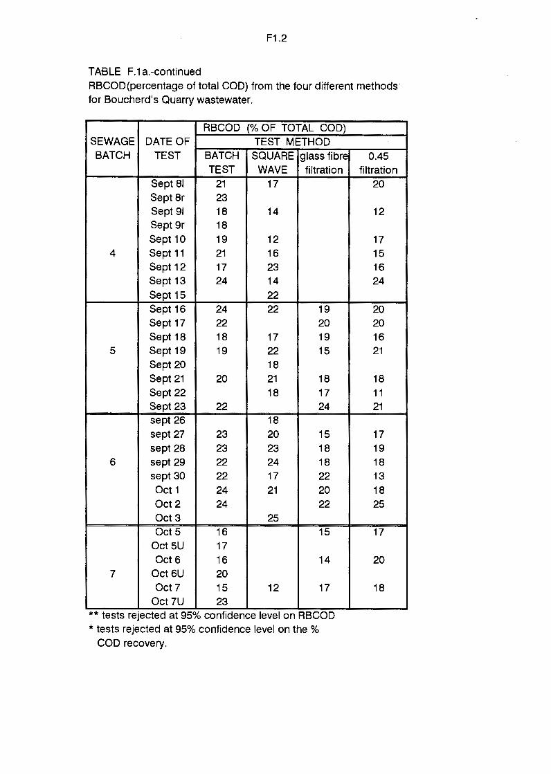
F1 .2
TABLE F.1a.-continued RBCOD(percentage of total COD) from the four different methods for Boucherd's Quarry wastewater.
RBCOD (% OF TOTAL COD) SEWAGE DATE OF TEST METHOD BATCH TEST BATCH SQUARE glass fibre
TEST WAVE filtration Sept 81 21 17 Sept Br 23 Sept 91 18 14 Sept 9r 18 Sept 10 19 12
4 Sept 11 21 16 Sept 12 17 23 Sept13 24 14 Sept 15 22 Sept 16 24 22 19 Sept17 22 20 Sept 18 18 17 19
5 Sept 19 19 22 15 Sept 20 18 Sept 21 20 21 18 Sept 22 18 17 Sept23 22 24 sept 26 18 sept 27 23 20 15 sept 28 23 23 18
6 sept 29 22 24 18 sept 30 22 17 22 Oct 1 24 21 20 Oct2 24 22 Oct 3 25 Oct 5 16 15
Oct5U 17 Oct6 16 14
7 Oct 6U 20 Oct 7 15 12 17
Oct 7U 23 ** tests rejected at 95% confidence level on RBCOD * tests rejected at 95% confidence level on the%
COD recovery.
0.45 filtration
20
12
17 15 16 24
20 20 16 21
18 11 21
17 19 18 13 18 25
17
20
18

F1 .3
TABLE F.1a.-continued RBCOD(percentage of total COD) from the four different methods for Boucherd's Quarry wastewater.
RBCOD (% OF TOTAL COD) SEWAGE DATE OF TEST METHOD BATCH TEST BATCH SQUARE glass fibre
TEST WAVE filtration Oct 8 16 18 20 Oct9 20 23 18
7 Cont. Oct 10 23 15 16 Oct 11 20 Oct 12 20 Oct 13 Oct 14 16 Oct 16 23 Oct 17 19 Oct 18 17 Oct 19 14 Oct 20 13
8 Oct 21 14 Oct 221 18 13 Oct 22r 16 Oct 23 15 Oct 24 16 16 Oct 251 11 17 Oct 25r 22 Oct 26 21 12 Oct 27 17 15 12 Oct 28 21 17 16 Oct 28 23 Oct 28 25 Oct 29 16 15 Oct 30 20 17
** tests rejected at 95% confidence level on RBCOD * tests rejected at 95% confidence level on the %
COD recovery.
0.45 filtration
15 14 16
12 11 14
14 17

F1 .4
TABLE F.1a.-continued RBCOD(percentage of total COD) from the four different methods for Boucherd's Quarry wastewater.
RBCOD (% OF TOTAL COD) SEWAGE DATE OF TEST METHOD BATCH TEST BATCH SQUARE glass fibre
TEST WAVE filtration Oct 31 20 15 17 Nov 1 19 21 19 Nov2 17 23 17
9 Nov3 14 17 21 Nov4 17 18 23 Nov5 17 17 Nov6 14 15 11 Nov? 19 Nova 19* 19
** tests rejected at 95% confidence level on RBCOD * tests rejected at 95% confidence level on the%
COD recovery.
0.45 filtration
17 19 17 21 23 18 12
20

F1 .5
TABLE F.1 b. RBCOD(percentage of total COD) from the four different methods for Mitchell's Plain wastewater.
RBCOD (% OF TOTAL COD) SEWAGE DATE OF TEST METHOD BATCH TEST BATCH SQUARE glass fibre
TEST WAVE filtration jan 20 23 jan 21 27 jan 22 15 jan 23 20 14 jan 24 23 19 jan 25 15
10a jan 26 23 16 jan 27 22 18 jan 28 11 jan 30 21 Jan 31 21 12 feb 1 24 20 feb2 17 21 feb 4 14 21 feb 5 16 12 feb 6 16 16 23 feb 7 21 20 16
10 feb 8 16 15 15 feb 9 18 25** 15 feb 10 13 16 14 feb 11 15 17 22 feb 12 24 23 19 feb 13 13 18 18 feb 17 16 19 feb 18 16 17 16 feb 19 18 17 23 feb 20 18 22 21
11 feb 21 16 17 20 feb 22 16 20 14 feb 23 21 27 19 feb 24 25 15 feb 25 14 feb 26 19
** tests rejected at 95% confidence level on RBCOD * tests rejected at 95% confidence level on the %
COD recovery.
0.45 filtration
23 20 13 18 20 18 14 15 21
22 18 23 21 19 20 16 19 14 14 24 18 19 18 17 15 19 19 21 16 18 14

F1 .6
TABLE F.1 b.-continued RBCOD(percentage of total COD) from the four different methods for Mitchell's Plain wastewater.
RBCOD (% OF TOTAL COD) SEWAGE DATE OF TEST METHOD BATCH TEST BATCH SQUARE glass fibre
TEST WAVE filtration feb 27 15 feb 28 11 ** 14
11 cont. mar 1 9** 13 15 mar2 10 16
mar 18 22* 19 mar 19 20 27 18 mar20 21 21 24 mar 21 23 26
12 mar 22 16 23 12 mar23 22 17 mar 24 18 19 24 mar25 16 mar26 12* 16 16 mar 27 11 14 mar28 14* 15 12 apr1 23 17 22 apr2 22 18 18 apr3 24 19 20 apr4 26 17 22 apr5 26 23 23
13 apr6 20 22 21 apr7 29 22 21 apr8 36** 21 25 apr9 35** 23 26 apr10 25 20 19 apr11 26 26 apr12 21 apr13 25 18
** tests rejected at 95% confidence level on RBCOD * tests rejected at 95% confidence level on the%
COD recovery.
0.45 filtration
15 17
23 24 26 19 21 25 16 17 14 12 22 18 23 22 23 25 21 26 26 22 26

F1 .7
TABLE F.1 b.- continued RBCOD(percentage of total COD) from the four different methods for Mitchell's Plain wastewater.
RBCOD (% OF TOTAL COD) SEWAGE DATE OF TEST METHOD BATCH TEST BATCH SQUARE glass fibre 0.45
TEST WAVE filtration filtration apr19 20 24 24 apr20 15 22 21 apr 21 16 16 18 18 apr22 16 26 22 apr23 19 19 apr24 20 17 22 18 apr25 28 22 22 apr26 26 18 20
14 apr27 21 21 apr28 26* 21 21 apr29 17 26 25 apr30 16 may? 22 12 may8 20 11 may9 16 21 18 may 10 13 21 21 may 11 23 22 24 may 12 18 14 17 17 may 13 21 21 may 14 25 20 may 15 22 22 may16 25 21 may 19 22 22 23 may20 19 14 19 may 21 17 14 14 may22 21 20 18
15 may23 21 18 16 may 24 22 24 23 may25 23 18 may26 21 21 may27 14 16 17 may28 17 14 may29 16 17 may30 18 16 16 may31 16 15
** tests rejected at 95% confidence level on RBCOD

F1 .8
TABLE F.1 b.- continued
RBCOD(percentage of total COD) from the four different methods for Mitchell's Plain wastewater.
RBCOD (% OF TOTAL COD) SEWAGE DATE OF TEST METHOD
BATCH TEST BATCH SQUARE glass fibre TEST WAVE filtration
june 12 24 june 13 20 june 14 23 june 15 20 june 17 18 june 19 21 june 20 20
16 june 21 25 june 23 22 19 17 june 24 15 17 19 june 25 23 june 26 28 20 20 june 27 26 25 19 june 28 18 17 june 29 25 24 20 june 30 23 22 15 july 1 16 18 24 july 2 17 july 3 25 july 4 24 20 17 july 5 27 21 21 july 6 21 19 july 7 35** 25 20 july 8 26 24 15
17 july 9 31 30 july 10 26 july 11 23 july 12 27 22 18 july 13 30 25 13 july 14 27 23 july 15 28 21 14 july 16 27 23 19
** tests rejected at 95% confidence level on RBCOD * tests rejected at 95% confidence level on the%
COD recovery.
0.45 filtration
16 20
20 18 17 18 15 19
18 18 17 20 19
18 17
20 21
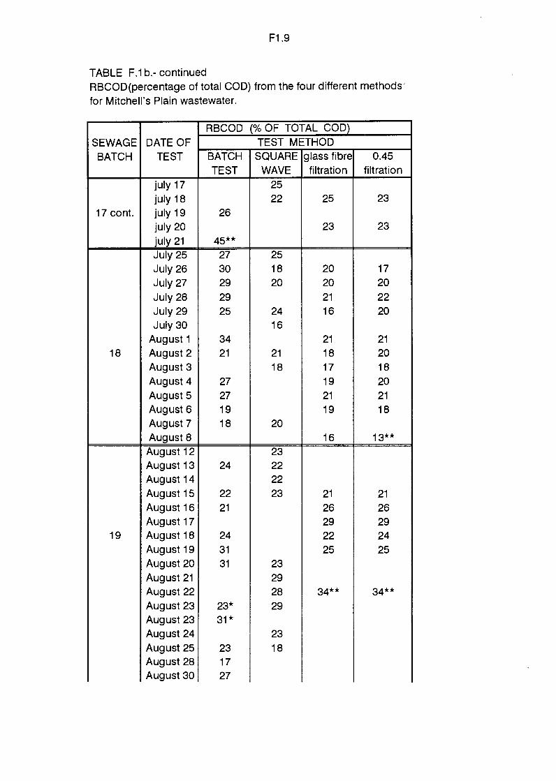
F1 .9
TABLE F.1 b.- continued RBCOD(percentage of total COD) from the four different methods for Mitchell's Plain wastewater.
RBCOD (% OF TOTAL COD)
SEWAGE DATE OF TEST METHOD BATCH TEST BATCH SQUARE glass fibre 0.45
TEST WAVE filtration filtration july 17 25 july 18 22 25 23
17 cont. july 19 26 july 20 23 23
july 21 45** July 25 27 25 July 26 30 18 20 17 July 27 29 20 20 20 July 28 29 21 22 July 29 25 24 16 20 July 30 16
August 1 34 21 21 18 August 2 21 21 18 20
August 3 18 17 18 August 4 27 19 20 August 5 27 21 21 August 6 19 19 18 August 7 18 20 August 8 16 13**
August 12 23 August 13 24 22 August 14 22 August 15 22 23 21 21 August 16 21 26 26 August 17 29 29
19 August 18 24 22 24 August 19 31 25 25 August 20 31 23 August 21 29 August 22 28 34** 34** August 23 23* 29 August 23 31* August 24 23 August 25 23 18 August 28 17 August 30 27

F1 .10
TABLE F.1 b.- continued RBCOD(percentage of total COD) from the four different methods for Mitchell's Plain wastewater.
RBCOD (% OF TOTAL COD) SEWAGE DATE OF TEST METHOD BATCH TEST BATCH SQUARE glass fibre
TEST WAVE filtration Sept 1 Sept 2 23 Sept 3 Sept4 25 Sept 5 20 Sept 6 23 Sept 7 27 16 25
20 Sept 8 16 23 26 Sept 9 24 23 25
Sept 11 22 22 23 Sept 12 15 20 Sept13 20 16**
Sept13L 17 Sept 14 23 Sept15 21 27 25 Sept 16 15** 22 Sept 17 17 Sept 18 Sept 19 16 19 Sept 20 13 Sept 21 17 22 16 Sept 22 19
21 Sept 23 22 15 Sept23 21 Sept 24 22 Sept 25 26 Sept 26 21 16 Sept 27 22 22 15 Sept 27 21 Sept 28 23 18 Sept 29 17 Sept 30 20 15
** tests rejected at 95% confidence level on RBCOD * tests rejected at 95% confidence level on the %
COD recovery.
0.45 filtration
20
25 26 25 23 20
16**
23 25
19 13 16 19 15
16 15
18 16 15

F1 .11
TABLE F.1 b.- continued RBCOD(percentage of total COD) from the four different methods for Mitchell's Plain wastewater.
RBCOD (% OF TOTAL COD) SEWAGE DATE OF TEST METHOD BATCH TEST BATCH SQUARE glass fibre
TEST WAVE filtration Sept30 19
21 cont. Oct 1 17 Oct 2 15 oct 21 16 oct 21 16 Oct 24 22 oct 25 14 oct 25 17 Oct 26 20 Oct 27 12
23 Oct 28 18 18 Oct 28 9** Oct 29 13 Oct30 12 Oct 31 25 Nov 1 24 Nov3 19 Nov3 22 Nov3 25 27
** tests rejected at 95% confidence level on RBCOD * tests rejected at 95% confidence level on the %
COD recovery.
0.45 filtration

APPENDIX G
DATA ON UNBIODEGRABLE SOLUBLE COD FROM THE BATCH TEST AND ACTIVATED SLUDGE SYSTEM EFFLUENT
TABLE OF CONTENTS
Table Gl: Comparison of unbiodegradable soluble COD from batch test and activated sludge system effluent.
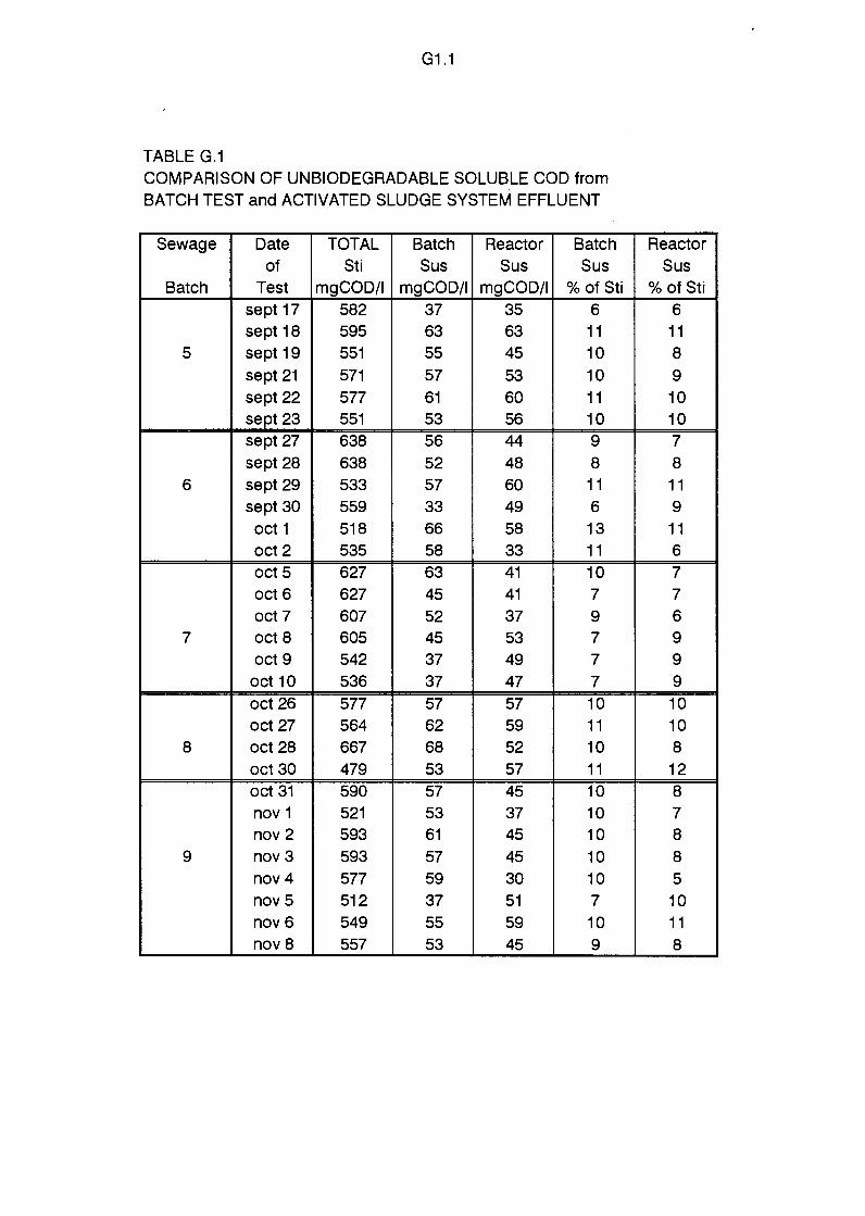
G1 .1
TABLE G.1 COMPARISON OF UNBIODEGRADABLE SOLUBLE COD from BATCH TEST and ACTIVATED SLUDGE SYSTEM EFFLUENT
Sewage Date TOTAL Batch Reactor Batch of Sti Sus Sus Sus
Batch Test mgCOD/1 mgCOD/1 mgCOD/1 % of Sti sept 17 582 37 35 6 sept 18 595 63 63 11
5 sept 19 551 55 45 10 sept 21 571 57 53 10 sept 22 577 61 60 11 sept 23 551 53 56 10 sept 27 638 56 44 9 sept 28 638 52 48 8
6 sept 29 533 57 60 11 sept 30 559 33 49 6 oct 1 518 66 58 13 oct 2 535 58 33 11 oct 5 627 63 41 10 oct 6 627 45 41 7 oct 7 607 52 37 9
7 oct 8 605 45 53 7 oct 9 542 37 49 7
oct 10 536 37 47 7 oct 26 577 57 57 10 oct 27 564 62 59 11
8 oct 28 667 68 52 10 oct 30 479 53 57 11 oct 31 590 57 45 10 nov 1 521 53 37 10 nov 2 593 61 45 10
9 nov 3 593 57 45 10 nov 4 577 59 30 10 nov 5 512 37 51 7 nov 6 549 55 59 10 nov 8 557 53 45 9
Reactor Sus
% of Sti 6
11 8 9
10 10 7 8
11 9
11 6 7 7 6 9 9 9 10 10 8 12 8 7 8 8 5
10 11 8

G1.2
TABLE G.1 -continued COMPARISON OF UNBIODEGRADABLE SOLUBLE COD from BATCH TEST and ACTIVATED SLUDGE SYSTEM EFFLUENT
Sewage Date TOTAL Batch Reactor Batch of Sti Sus Sus Sus
Batch Test mgCOD/1 mgCOD/1 mgCOD/1 % of Sti feb 5 456 51 37 11 feb 6 456 37 37 8 feb 7 456 43 37 9 feb 8 460 40 42 9
10 feb 9 520 56 48 11 feb 10 524 54 42 10 feb 11 484 44 50 9 feb 12 540 34 46 6 feb 13 544 10 24 2 feb 23 526 45 43 8 feb 24 621 37 37 6
11 feb 25 503 47 49 9 mar 1 539 58 57 11 mar2 552 57 47 10
mar 18 459 53 33 12 mar 19 455 51 53 11 mar 20 480 41 24 9 mar 21 480 40 28 8 mar 22 512 41 49 8
12 mar23 585 57 49 10 mar24 514 22 22 4 mar25 514 49 47 10 mar26 514 57 55 11 mar27 681 49 61 7 mar 28 588 43 49 7
Reactor Sus
% of Sti 8 8 8 9 9 8 10 9 4
8 6 10 11 9 7 12 5 6 10 8 4 9
11 9 8

G1.3
TABLE G.1 -continued COMPARISON OF UNBIODEGRADABLE SOLUBLE COD from BATCH TEST and ACTIVATED SLUDGE SYSTEM EFFLUENT
Sewage Date TOTAL Batch Reactor Batch of Sti Sus Sus Sus
Batch Test mgCOD/1 mgCOD/1 mgCOD/1 % of Sti apr1 570 77 30 14 apr3 524 38 35 7 apr4 581 53 37 9 apr5 506 39 37 8 apr6 545 59 33 11
13 apr7 502 59 55 12 apr8 518 45 37 9 apr9 554 57 28 10 apr10 603 53 45 9 apr11 574 24 33 4 apr12 574 49 20 9 apr13 554 45 41 8 apr19 685 57 27 8 apr20 587 41 39 7 apr 21 664 52 41 8 apr22 607 53 37 9 apr23 636 52 45 8
14 apr24 624 54 53 9 apr25 624 45 37 7 apr26 624 60 60 10 apr28 504 61 44 12 apr29 645 52 35 8 may 11 552 47 41 8 may 12 605 51 51 8 may 13 642 51 47 8 may 15 560 38 47 7 may 16 626 44 30 7 may 18 605 38 42 6 may 19 432 41 22 9
15 may 21 541 51 47 9 may22 521 44 47 9 may23 586 45 53 8 may24 472 37 37 8 may25 456 41 39 9 may 27 612 27 31 4 may30 525 29 23 5
Reactor Sus
% of Sti 5 7 6 7 6
11 7 5 7 6 4 7 4 7 6 6 7 9 6 10 9 5 7 8 7 8 5 7 5 9 9 9 8 9 5 4

G1 .4
TABLE G.1 -continued COMPARISON OF UNBIODEGRADABLE SOLUBLE COD from BATCH TEST and ACTIVATED SLUDGE SYSTEM EFFLUENT
Sewage Date TOTAL Batch Reactor Batch
of Sti Sus Sus Sus Batch Test mgCOD/1 mgCOD/1 mgCOD/1 % of Sti
June 23 461 36 34 8 June 24 469 54 28 12 June 26 497 48 26 10
16 June 27 533 36 32 7 June 29 441 28 26 6 June 30 545 48 20 9 July 1 464 36 12 8 July4 556 38 32 7 July 5 504 50 48 10 July 6 516 54 24 11 July 7 492 24 32 5 July 8 556 37 36 7 July 9 504 52 52 10
July 12 530 40 52 8 17 July 13 514 45 36 9
July 14 534 45 36 8 July 15 567 49 45 9 July 16 551 53 49 10 July 18 461 61 24 13 July 19 486 12 41 3 July 21 477 37 34 8 July 25 469 37 37 8 July 27 545 29 24 5 July 28 555 43 33 8 July 29 451 43 33 10
18 Aug 1 437 25 25 6 Aug 2 519 25 29 5 Aug 4 503 49 49 10 Aug 5 443 49 57 11 Aug 6 511 41 33 8 Aug 7 510 41 33 8
Reactor Sus
% of Sti 7 6 5 6 6 4 3 6
10 5 7 6 10 10 7 7 8 9 5 8 7 8 4 6 7 6 6 10 13 6 6

G1.5
TABLE G.1 -continued COMPARISON OF UNBIODEGRADABLE SOLUBLE COD from BATCH TEST and ACTIVATED SLUDGE SYSTEM EFFLUENT
Sewage Date TOTAL Batch Reactor Batch
of Sti Sus Sus Sus Batch Test mgCOD/1 mgCOD/1 mgCOD/1 % of Sti
Aug 16 545 37 33 7 19 Aug 18 480 45 45 9
Aug 19 511 33 45 6 Aug 20 579 56 37 10 Aug28 584 39 43 7 Aug 30 567 39 29 7 Sept 2 606 47 41 8 Sept 4 526 49 41 9 Sept 6 520 41 41 8 Sept 7 520 27 23 5
20 Sept 8 543 31 41 6 Sept9 508 41 31 8
Sept 11 483 53 37 11 Sept 13r 525 35 33 7 Sept 131 525 45 33 9 Sept15 411 41 27 10
Sept 16 * 484 33 25 7 Sept 19 583 44 33 8 Sept 21 548 37 27 7
21 Sept 231* 511 43 41 8 Sept 23r 511 55 41 11 Sept 27r 556 41 45 7
Sept 271 * 556 43 45 8 Sept 30r 523 49 24 9 Sept 30I* 523 26 24 5 13 Oct 664 36 36 5 13 Oct s 1040 36 36 3
25 Oct{4) 561 45 45 8 25 Oct(3) 561 41 45 7
22 28 Oct(4) 506 43 33 8 28 Oct(3) 506 53 33 10 3 Nov(2) 539 63 55 12 3 Nov(3) 539 37 55 7 3 Nov(4) 539 41 55 8
Reactor Sus
% of Sti 6 9
9 6 7 5 7 8 8 4 8 6 8 6 6 6 5 6 5 8 8 8 8 5 5 5 3 8 8 6 6 10 10 10

APPENDIXH
PROCEDURE FOR THE BATCH TEST METHOD
TABLE OF CONTENTS
H.1 INTRODUCTION H.2 TEST PROCEDURE

APPENDIXH
PROCEDURE FOR THE BATCH TEST METHOD
H.l INTRODUCTION
In this investigation a batch test procedure has been developed to quantify the five
influent COD fractions, heterotroph active biomass, readily biodegradable COD
(RBCOD), unbiodegradable soluble COD, slowly biodegradable COD (SBCOD),
and unbiodegradable particulate COD. The accuracy of these estimates for the five
influent fractions has been described in detail in Chapters 5, 7 and 9: The batch
test method provides good estimates for heterotroph active biomass, RBCOD and
unbiodegradable soluble COD; the estimates for unbiodegradable particulate COD
as a fraction of total COD (fup) tend to be higher than those from conventional
tests, and consequently the estimate for SBCOD tends to be lower - it remains to
be evaluated whether these trends are consistent.
For all the COD fractions derived from the batch test, the accuracy of the values
hinges around the accuracy of the experimental data. To obtain acceptable data,
the experimental investigation must be conducted with an uncompromising
vigilance, a strict discipline and attention to detail and measurements in every
aspect; if these are lax or neglected, the results will be largely useless. To facilitate
application of the batch test, the procedure for the entire test will be set out in
detail.
H.2 TEST PROCEDURE
(1) A sample of raw (unsettled) municipal wastewater is obtained from the
source. A defined volume is placed in a continuously stirred batch reactor
maintained at a constant temperature of 20° C. Other temperatures may be
suitable for the batch test, but this has not been investigated. The
wastewater may be diluted or undiluted; in this investigation, the wastewater
was diluted to ±500 mgCOD/t, so that the oxygen utilization rates could be
readily measured.
(2) A sample is drawn from the batch reactor and the initial total COD
concentration determined (Standard Methods, 1985).

H.2
(3) The surface of the wastewater in the reactor is covered, to limit surface
exchange of oxygen. In this investigation, small hollow plastic balls (20 mm
diameter) were found to be most suitable.
( 4) The oxygen utilization rate ( 0 UR) is monitored continually. In this
investigation, the automated technique of Randall et al. (1991) was used: The
DO was raised to a high DO set point (±6,0 mgO/l), the air was switched off
and the decrease in DO with time monitored. The slope of the DO-time
profile defines the OUR and this was automatically recorded. When the DO
reached a low DO set point (±2,0 mgO/l), the air was turned on and the
cycle repeated.
(5) During an aeration cycle, the aeration rate should be sufficient to ensure that
the DO can be raised from the low to the high DO concentration set points
without excessive delay, but should not be over vigorous, to limit splashing.
(6) The pH of the batch reactor is monitored and controlled to pH 7,5 ( ±0,2).
(7) Intermittently, the walls of the reactor are thoroughly brushed during an
aeration cycle to prevent particulate matter adhering to them.
(8) In order to check for nitrification, at regular intervals samples are drawn from
the reactor, filtered (0,45µm) and analyzed for nitrate and nitrite. Should
nitrification be detected, allyl thiourea probably can be used as nitrification
inhibitor ( due to absence of nitrification, addition of ally I thiourea was not
tested in this investigation).
(9) If influent RBCOD and heterotroph active biomass only are to be determined,
the batch test is run until the precipitous drop in OUR is observed, and then
for a further two hours. The walls of the reactor and the stirrers are brushed
of any particulate matter sticking on to them. The mixed liquor is then
drawn from the batch reactor, poured into a liquidizer and homogenized. A
sample is taken from the homogenized mixed liquor for the determination of
total COD (Standard Methods, 1985) at the end of the test, in order to
determine the% COD recovery [Eq (4.1), Chapter 4].
(10) If unbiodegradable soluble COD concentration is to be determined as well, the

H.3
batch test is run for 1 day, and then treated as in step (9) above. In
addition, a representative sample (say 500 mt) of the homogenized liquor is
drawn off, dosed with 5 mt of aluminium sulphate (stock solution of 50 g/t),
stirred rapidly ( :1:200 rpm) for 2 minutes and then left to settle for 30 minutes
with slow stirring ( :1:2 rpm). A sample is taken from the clear liquid, filtered
through glass fibre filter paper and the COD of the filtrate determined
(Standard Methods, 1985); this gives the unbiodegradable soluble COD
concentration. It was noted in this investigation that the duration of running
the test after the precipitous drop does not affect the concentration of this
parameter, provided the length of the batch test > 1 day.
(11) If unbiodegradable particulate and slowly biodegradable COD are to be
determined, the batch test is run for a total of 2 days, after which a third of
the thoroughly mixed contents of the batch reactor are drawn off and treated
as in steps (9) and (10) above, to determine total and unbiodegradable soluble
COD concentrations. The volume of mixed liquor remaining in the batch
reactor is noted, and flocculated-filtered raw wastewater ( as described below)
is added to bring the batch reactor back to its original volume.
Preparation of the flocculated-filtered wastewater for addition to the batch
reactor is as follows:
Raw wastewater from the same source being tested is dosed with aluminium
sulphate by adding 20 mt of stock aluminium sulphate (stock at
concentration of 50 g/t) to 5 litres of wastewater and thoroughly mixed.
The mixture is allowed to settle for 1 hour or longer. The clear supernatant
liquid is filtered through glass fibre filter paper (Whatman's GF /C), and
the filtrate is added to the batch reactor, as described above.
The batch test is continued until a second precipitous drop in the OUR is
noted. The total and . unbiodegradable COD concentrations are then
determined [ as in steps ( 9) and ( 10) above respectively] .
(12) From the data, RBCOD and heterotroph active biomass are calculated using
the procedures set out in Chapter 4, the unbiodegradable soluble COD is
flocculated filtrate COD in step (10), and unbiodegradable particulate and
SBCOD are calculated using the procedures in Chapter 8, Section 8.8.