characterization of fluidization regimes by analysis …

CHARACTERIZATION OF FLUIDIZATION REGIMES

BY ANALYSIS OF PRESSURE FLUCTUATIONS IN GAS-

SOLID FLUIDIZED BEDS

Sayuri Naidoo

Submitted in fulfilment of the requirements for the degree of

Master of Science in Engineering at the School of Chemical Engineering,

University of KwaZulu-Natal

2017

LIBRARY COPY

iii

ACKNOWLEDGEMENTS

I wish to acknowledge my supervisors and the technical staff, whose guidance and assistance I

really appreciated during the course of this project.

I wish to thank my husband and family for your love and support, I am truly grateful.

iv

ABSTRACT

Fluidized beds are ranked as the top contacting method with the best overall benefits, and have

been used over many years in several industrial applications. Literature indicates that pressure

fluctuations are influenced by variables related to fluidization regimes in a fluidized bed; such

as the bubble size, bubbling rising velocity and the motion of the bed surface (Fan et al., 1981).

Hence several researchers have employed pressure fluctuations to aid in the understanding of

fluidized bed system hydrodynamics.

This study was focused on gas-solid fluidized beds, during aggregative fluidization represented

by the bubbling, slugging and turbulent regimes. Geldart (1973) materials from the

classification were studied in this research; Group A (spent Fluid Cracking Catalyst), Group B

(sand) and Group D (plastic beads). The experimental equipment was composed of an existing

laboratory-scale gas-solid fluidized bed and data acquisition system. Three transparent fluidized

bed columns were investigated; fluidized bed 1 (I.D 5 cm), fluidized bed 2 (I.D 11 cm) and

fluidized bed 3 (I.D 29 cm). The time-series analysis of pressure fluctuation signals were

investigated using the time and frequency domain methods. The pressure fluctuation signal was

converted into the frequency domain by use of the Fast Fourier Transform (FFT).

For increased bed heights the power spectrum was narrower, higher in amplitude, had more

distinct peaks and the dominant frequency was lower, when compared to the lower bed height

for the same material and fluidization regime. Also decreasing dominant frequencies and large

increases in the amplitude of the pressure fluctuation were observed for each increasing

fluidization regime; from the bubbling to slugging and to the turbulent regimes. The research

contribution from this study was realized, as a range of dominant frequencies were successfully

identified for each specific fluidization regime at its respective velocities. The identification of

the transition phase was accomplished with low accuracy from the research contribution. It was

recommended to employ differential pressure measurements for larger columns to increase the

accuracy of data achieved; thereby permitting the comparison of useable power spectra results

for scale-up.

v

TABLE OF CONTENTS

ACKNOWLEDGEMENTS ......................................................................................................... iii

ABSTRACT ................................................................................................................................. iv

TABLE OF CONTENTS .............................................................................................................. v

LIST OF FIGURES ................................................................................................................... viii

LIST OF TABLES ....................................................................................................................... xi

NOMENCLATURE .................................................................................................................... xii

1. INTRODUCTION .................................................................................................................... 1

1.1 Background and Relevance ................................................................................................. 1

1.2 Project Aims and Objectives ............................................................................................... 3

1.3 Research Contributions ....................................................................................................... 4

1.4 Outline of Dissertation ........................................................................................................ 4

2. LITERATURE REVIEW ......................................................................................................... 5

2.1 Fluidization ............................................................................................................................. 5

2.1.1 Fluidization in Industry .................................................................................................... 5

2.1.2 Fluidized Beds ................................................................................................................. 6

2.1.3 Fluidization Regimes ....................................................................................................... 8

2.1.4 Geldart Powder Classification ....................................................................................... 11

2.1.5 Minimum Fluidization Voidage ..................................................................................... 13

2.1.6 Minimum Fluidization Velocity .................................................................................... 14

2.1.7 Minimum Bubbling Velocity ......................................................................................... 17

2.1.8 Minimum Slugging Velocity ......................................................................................... 18

2.1.9 Transition Phase between the different Fluidization Regimes ...................................... 19

2.2 Methods for Analysis of Pressure Fluctuations..................................................................... 21

2.2.1 Time Domain Analysis .................................................................................................. 21

2.2.2 Frequency Domain Analysis .......................................................................................... 23

2.2.3 State Space Domain Analysis ........................................................................................ 26

2.3 Scale Up ................................................................................................................................ 27

3. EXPERIMENTAL EQUIPMENT .......................................................................................... 29

vi

3.1 The Gas-Solid Fluidized Bed Apparatus .......................................................................... 29

3.1.1 Fluidized Bed ............................................................................................................. 33

3.1.2 Bed Height ................................................................................................................. 33

3.1.3 Distributor .................................................................................................................. 33

3.1.4 Plenum Chamber ....................................................................................................... 34

3.1.5 Flow Measurement and Control ................................................................................ 34

3.1.6 Pressure Measurement and Control ........................................................................... 35

3.2 Particle Size Analysis Equipment ..................................................................................... 36

4. EXPERIMENTAL METHODS .............................................................................................. 38

4.1 Particle Selection and Characterization ............................................................................ 38

4.1.1 Particle Selection ....................................................................................................... 38

4.1.2 Particle Characterization ............................................................................................ 38

4.1.2.1 Particle Density ..................................................................................................... 39

4.1.2.2 Particle Size .......................................................................................................... 40

4.2 Preparation of the Gas-Solid System Equipment.............................................................. 41

4.2.1 Changing of Material ................................................................................................. 41

4.2.2 Back Flow of Material ............................................................................................... 41

4.3 Operation of the Gas-Solid System Equipment ................................................................ 41

4.4 Measuring and Processing of Pressure Fluctuation Signals ............................................. 44

5. RESULTS AND DISCUSSION ............................................................................................. 45

5.1 Experimental Observations ............................................................................................... 45

5.2 Analysis in the Time Domain ........................................................................................... 46

5.2.1 Time-Pressure Analysis ............................................................................................. 46

5.2.2 Predicted Minimum Fluidization Regime Velocity ................................................... 49

5.2.3 Predicted and Experimental Fluidization Regime Transition Velocity ..................... 52

5.3 Analysis in the Frequency Domain ................................................................................... 54

5.3.1 Power Spectral Analysis ............................................................................................ 54

5.3.2 Summary of the Frequency Domain Analysis ........................................................... 58

5.3.2.1 Fluidized Bed 1 .................................................................................................... 58

vii

5.3.2.2 Fluidized Bed 2 .................................................................................................... 60

5.3.2.3 Fluidized Bed 3 .................................................................................................... 65

5.4 Comparison to Literature Data ......................................................................................... 67

5.5 Applicability for Scale Up ................................................................................................ 69

6. CONCLUSIONS ..................................................................................................................... 71

7. RECOMMENDATIONS ........................................................................................................ 75

REFERENCES............................................................................................................................ 77

APPENDIX A: ADDITIONAL TIME DOMAIN RESULTS .................................................... 80

APPENDIX B: ADDITIONAL FREQUENCY DOMAIN RESULTS ...................................... 85

APPENDIX C:MATLAB CODE FOR IMPLEMENTATION OF THE FAST FOURIER

TRANSFORM ............................................................................................................................ 87

APPENDIX D: PARTICLE SIZE RESULTS ............................................................................ 90

viii

LIST OF FIGURES

Chapter 2:

Figure 2.1: Schematic of the components of a fluidized bed (Pell, 1990) .................................... 8

Figure 2.2: Schematic of the different fluidization regimes that exist with increasing gas

velocity, adapted from Grace (1982) .......................................................................................... 11

Figure 2.3: Geldart classification of powders (Geldart, 1973) .................................................... 13

Figure 2.4: Bed expansion at minimum fluidization conditions (Kunii & Levenspiel, 1991) .... 15

Figure 2.5: The amplitude of pressure fluctuation against the increasing gas velocity (Basu,

2006) ........................................................................................................................................... 20

Figure 2.6: Time-series of the bubbling regimes using sand with a 290 μm diameter in fluidized

bed column of 11.5 cm at a bed height of 11 cm (Alberto et al., 2004) ...................................... 22

Figure 2.7: Power spectra of the bubbling regime using sand with a 290 μm diameter in

fluidized bed column of 11.5 cm at a bed height of 11 cm (Alberto et al., 2004) ...................... 24

Chapter 3:

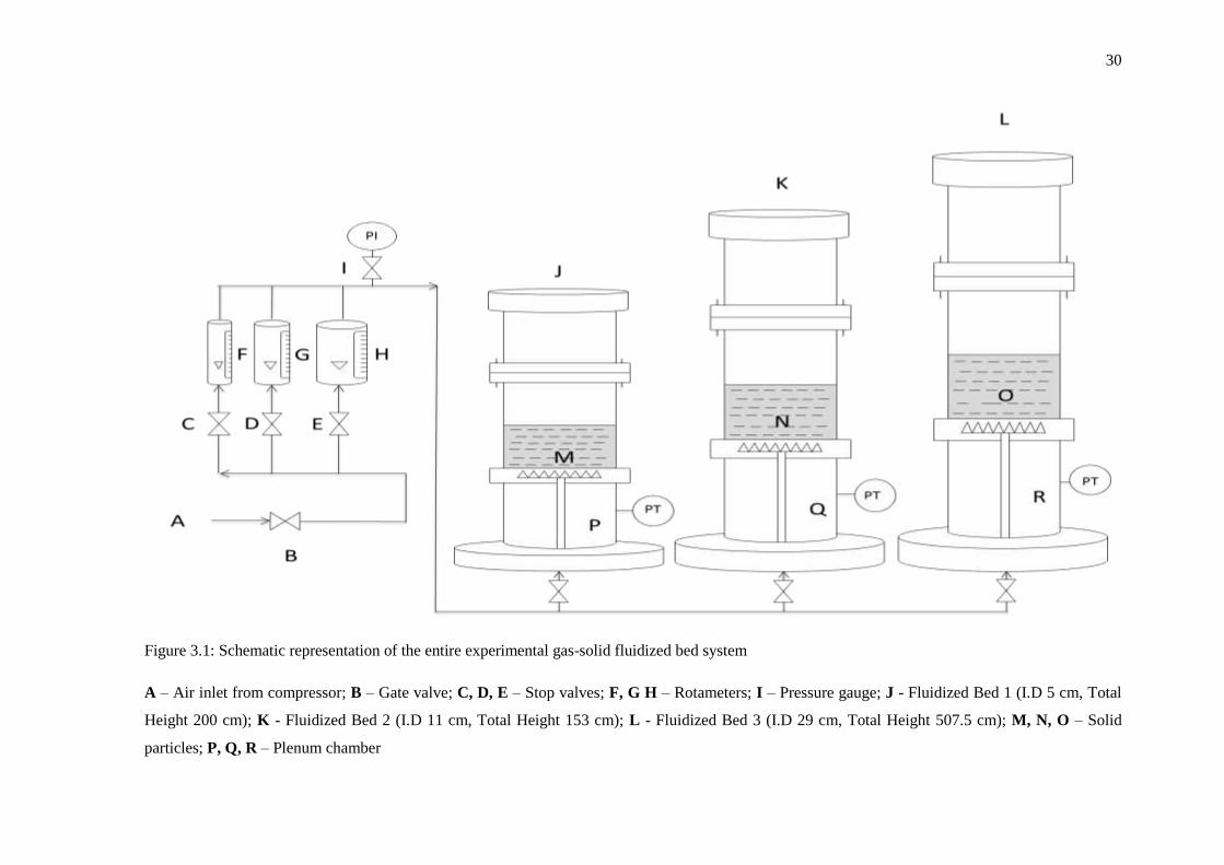
Figure 3.1: Schematic representation of the entire experimental gas-solid fluidized bed system

..................................................................................................................................................... 30

Figure 3.2: Schematic representation of the experimental gas-solid fluidized bed system ......... 31

Figure 3.3: Lab-scale gas-solid fluidized bed system ................................................................. 32

Figure 3.4: Shimadzu SALD-3101 laser diffraction particle size analyser used to measure

Geldart Group A particles (spent FCC) ...................................................................................... 36

Figure 3.5: Vibrating screen shaker with test sieves used to measure Geldart Group B particles

(sand) ........................................................................................................................................... 37

Chapter 5:

Figure 5.1: Time-series of the pressure fluctuations measured in the three regimes using sand in

fluidized bed 2 at a bed height of 11 cm ..................................................................................... 48


fluidized bed 2 at a bed height of 21 cm ..................................................................................... 48

Figure 5.3: Standard deviation of pressure fluctuation with increasing superficial gas velocity

for sand in fluidized bed 2 with a bed height of 11 cm ............................................................... 54

Figure 5.4: Power spectra of the bubbling regime using sand in fluidized bed 2 at a bed height of

11 cm (A) and bed height of 21 cm (B) ...................................................................................... 56

ix

Figure 5.5: Power spectra of the slugging regime using sand in fluidized bed 2 at a bed height of

11 cm (A) and bed height of 21 cm (B) ...................................................................................... 57

Figure 5.6: Power spectra of the turbulent regime using sand in fluidized bed 2 at a bed height

of 11 cm (A) and bed height of 21 cm (B) .................................................................................. 57

Figure 5.7: Summary of the relationship between the dominant frequency and the superficial gas

velocity for the slugging and turbulent regime using sand in fluidized bed 1 at a bed height of 30

cm ................................................................................................................................................ 59


velocity for the bubbling regime using spent FCC in fluidized bed 2 at a bed height of 11 cm

and 21 cm .................................................................................................................................... 61


velocity for all fluidization regimes using sand in fluidized bed 2 at a bed height of 11 cm ...... 62

Figure 5.10: Summary of the relationship between the dominant frequency and the superficial

gas velocity for all fluidization regimes using sand in fluidized bed 2 at a bed height of 21 cm 63


gas velocity for the bubbling and slugging regime using plastic beads in fluidized bed 2 at a bed

height of 11 cm ........................................................................................................................... 64



height of 21 cm ........................................................................................................................... 65


gas velocity for the bubbling regime using spent FCC in fluidized bed 3 at a bed height of 29 cm

..................................................................................................................................................... 66


gas velocity for the bubbling regime using sand in fluidized bed 3 at a bed height of 32 cm .... 67

Figure 5.15: Power spectra of the bubbling regime using spent FCC (A) particle size 92 μm, bed

height 20.5 cm and column I.D 11.15 cm; (Alberto et al., 2004) and (B) particle size 87 μm,

bed height 21 cm and column I.D 11 cm; (Experimental) .......................................................... 68

Appendix A:

Figure A.1: Time-series of the pressure fluctuations measured in the bubbling regime using

spent FCC in fluidized bed 2 at the indicated bed heights .......................................................... 80

Figure A.2: Time-series of the pressure fluctuations measured in the bubbling regime using sand

in fluidized bed 2 at the indicated bed heights ............................................................................ 81

Figure A.3: Time-series of the pressure fluctuations measured in the slugging regime using sand

in fluidized bed 2 at the indicated bed heights ............................................................................ 81

x

Figure A.4: Time-series of the pressure fluctuations measured in the turbulent regime using

sand in fluidized bed 2 at the indicated bed heights .................................................................... 82

Figure A.5: Time-series of the pressure fluctuations measured in the transition from bubbling to

slugging regime using sand in fluidized bed 2 at the indicated bed heights ............................... 82

Figure A.6: Time-series of the pressure fluctuations measured in the transition from slugging to

turbulent regime using sand in fluidized bed 2 at the indicated bed heights ............................... 83


plastic beads in fluidized bed 2 at the indicated bed heights ...................................................... 83

Figure A.8: Time-series of the pressure fluctuations measured in the slugging regime using

plastic beads in fluidized bed 2 at the indicated bed heights ...................................................... 84


slugging regime using plastic beads in fluidized bed 2 at the indicated bed heights .................. 84

Appendix B:

Figure B.1: Power spectra of the bubbling regime using spent FCC in fluidized bed 2 at a bed

height of 11 cm (A) and bed height of 21 cm (B) ....................................................................... 85

Figure B.2: Power spectra of the bubbling regime using plastic beads in fluidized bed 2 at a bed


Figure B.3: Power spectra of the slugging regime using plastic beads in fluidized bed 2 at a bed


Appendix D:

Figure D.1: Geldart Group A (spent FCC) Shimadzu SALD-3101 laser diffraction particle size

analyser results…………………………………………………………… ……………………91

xi

LIST OF TABLES

Chapter 2:

Table 2.1: Minimum fluidization voidage adapted from Leva et al. (1951) ............................... 14

Table 2.2: Correlations to determine the minimum fluidization velocity ................................... 17

Table 2.3: Correlations to determine the minimum slugging velocity ........................................ 19

Table 2.4: Correlations to determine the transition velocity ....................................................... 20

Chapter 4:

Table 4.1: Particle characteristics of solid particles for gas-solid fluidization ........................... 40

Table 4.2: Operational conditions of gas-solid fluidized beds .................................................... 43

Chapter 5:

Table 5.1: Predicted results for the minimum fluidization velocity ............................................ 49

Table 5.2: Predicted results for the minimum slugging velocity from Stewart and Davidson

(1967) .......................................................................................................................................... 51

Table 5.3: Predicted results for the minimum slugging velocity from Baeyens and Geldart

(1974) .......................................................................................................................................... 51

Table 5.4: Predicted results for the minimum slugging velocity from Singh and Roy (2008) ... 52

Table 5.5: Predicted results for the transition velocity ................................................................ 53

Table 5.6: Summary of the comparison of the dominant frequency for material sand in all

fluidized bed columns ................................................................................................................. 69

xii

NOMENCLATURE

Notation Units

A Cross-sectional area m2

Ar Archimedes number -

D or Dc Column diameter m

Dp or dp Particle diameter m

F Mass fraction of solids with diameter < 45μm

FCC Fluid Catalytic Cracking -

Fr Froude‟s number -

f Frequency Hz

g Gravitational acceleration m/s2

H, L Bed height m

h Length of Cylinder m

I.D Internal column diameter m

m Mass kg

m Scale factor -

P Pressure Pa

R Rotameter reading L/min

Re Reynolds number -

t Time s

u Superficial gas velocity m/s

uc Start of transition regime velocity m/s

uk End of transition regime velocity m/s

xiii

umb Minimum bubbling velocity m/s

umf Minimum fluidization velocity m/s

ums Minimum slugging velocity m/s

ut Terminal velocity m/s

V Volume m3

Greek Letters

∆ Denotes change in a property -

ε Bed voidage -

ϕ Sphericity of solid particles -

ρ Density kg/m3

σ Standard deviation of pressure Pa

μ Viscosity of fluid Pa.s

Subscript

mb Minimum bubbling

mf Minimum fluidization

mf Minimum slugging

p Denotes a particle

s Denotes a solid

Superscript

0 Denotes the prototype

1

1

CHAPTER ONE

1. INTRODUCTION

1.1 Background and Relevance

Fluidization is defined as the conversion of a bed of solid particles into a fluid-like state,

through the contact of a fluidizing medium, either a gas or liquid, passing upward through the

bed (Kunii & Levenspiel, 1991). Fluidized beds are ranked as the top contacting method with

the best overall benefits, and it has been used over many years in several industrial applications.

Fluidization is applied to diverse sectors in industry such as the petro-chemical, energy

conversion, mineral processing and nuclear sectors. Some of the main advantages of fluidized

beds include the isothermal conditions achieved in reactors due to the rapid particle mixing,

high heat and mass transfer rates between gas and particles compared to other forms of

contacting, and their use in both small and large scale operations, since it allows for continuous

processing (Kunii & Levenspiel, 1991).

Fluidized beds have been used successfully in both catalytic and non-catalytic processes. Some

of these catalytic processes applications include hydrocarbon cracking and re-forming, as well

as the oxidation of naphthalene to phthalic anhydride. The non-catalytic processes include the

roasting of sulphides ores, coking of petroleum residues, incineration of sewage and drying of

solids (Perry & Green, 1997). Due to climate change and economic factors the need for clean

energy from fossil and biomass fuels has become increasingly important. Fluidized beds have

been found to be advantageous in reducing greenhouse gas emissions in the cement industry

2

applications (Basu, 2006). Therefore this study can contribute toward this climate change

initiative by improving the performance of fluidized beds.

Almost 31 years ago Geldart (1986) said “the arrival time of a space probe travelling to Saturn

can be predicted more accurately than the behaviour of a fluidized bed chemical reactor!”. This

still remains true to fluidization engineering today, therefore several studies have been dedicated

to the hydrodynamics and modelling of fluidized beds. To promote successful industry

applications and operations, it is vital to determine the fluidization regime best suited to that

specific process. Some fluidization regimes result in restricted heat and mass transfer, as well as

non-uniform bed mixing causing them to be undesirable. Therefore success is dependent on the

identification of a well-defined and stable fluidization regime.

At gas-solid fluidization there are various fluidization regimes that exist, such as the bubbling,

slugging and turbulent regimes. In the bubbling regime inefficient contacting of gas-solids can

occur due to large deviations from plug flow. However higher contacting efficiency is usually

achieved in the turbulent regime. Typically, the slugging regime can only occur in small

columns, where significant plant vibrations occur. This is avoided by the use of large industrial

operating units (Basu, 2006). Since the hydrodynamic state of fluidization is highly dependent

on the performance of the fluidized bed, it is imperative to identify the different fluidization

regimes. Visual observations are often impossible in large-scale industrial applications, since

columns are often constructed from non-transparent materials. Literature indicates that pressure

fluctuations, also referred to as the pressure drop, are influenced by variables related to

fluidization regimes in a fluidized bed, such as the bubble size, bubbling rising velocity and the

motion of the bed surface (Fan et al., 1981). Pressure fluctuations have been found to provide

information in the fluidized bed column due to its relationship to the state of fluidization (van

Ommen et al., 2011). Hence several researchers have employed pressure fluctuations to aid in

the understanding of a fluidized bed system hydrodynamics.

The ease of operability of pressure fluctuation measurement in a fluidized bed, even under

unfavourable industrial conditions, have made it one of the most common analysis methods for

fluidized beds studies (van Ommen et al., 2011). Pressure probes and transmitters measure the

pressure fluctuations along measuring points in the fluidized bed column, and this is connected

to a data acquisition system. Davidson et al. (1985) found that the points of pressure

measurement should be at the centre of the bed since the state of fluidization is fully developed

3

at this location. The interpretation of the pressure fluctuation signals is not direct; therefore

many researchers have been working on improving this technique. The time series analysis of

the pressure fluctuation signals in a fluidized bed can be used to give a quantitative description

of the different fluidization regimes using several methods. These methods can be separated into

three categories, such as the time domain analysis, the frequency domain analysis and the state-

space domain analysis (van Ommen et al., 2011). The analysis in the time domain denotes the

simplest approach, in which the standard deviation attained from the amplitude of pressure

fluctuation signals is often studied. The analysis in the frequency domain denotes the most

common approach, in which the power spectra obtained from the pressure fluctuations signals

are studied to obtain a dominant frequency. And the analysis in the state space domain is most

commonly used for non-linear analysis.

1.2 Project Aims and Objectives

Firstly, the time domain method will be evaluated for the classification of each fluidization

regime and credibility of the data received. The overarching aim of the study was to confirm

that the time-series analysis in the frequency domain, through the use of the Fast Fourier

Transform (FFT), could be used to characterize the different fluidization regimes in gas-

solid fluidized beds. Furthermore, the application and effectiveness of the frequency domain

technique will be verified in the transition phase regime.

Additionally, the study aimed to assess the various system variables such as particles

properties, bed properties and fluidizing medium properties, on the extent and transition

between these fluidization regimes.

The pressure probe location within a fluidized bed plays an integral role in generating

accurate, consistent and useable data. Thus the optimum location was also sought in this

study, whilst avoiding any possible obstruction to the measurement junction by solid

particles.

The final aim was established from a recommendation given by Gyan (2015); for the

applicability of scale up through tests conducted in larger columns.

4

1.3 Research Contributions

Research on pressure fluctuations in gas-solid fluidized beds, is mainly focused on observing a

single dominant frequency, at a specific superficial gas velocity for each of the different

fluidization regimes i.e. bubbling, slugging and turbulent regimes. The interpretation and

observation of the power spectra with the dominant frequency is different for every researcher.

Limited studies have been conducted for a range of superficial gas velocities occurring at the

same fluidization regime. This could provide further understanding into the application of the

method for industrial use, due to the gas velocity rarely being kept completely constant (van

Ommen et al., 2011). This study will report on the applicability and use of pressure fluctuations,

to determine a range of dominant frequencies occurring at a range of superficial gas velocities

for a specific fluidization regime.

1.4 Outline of Dissertation

The dissertation is arranged into seven chapters. A summary of the content contained in each

chapter is provided below.

Chapter 1 presents the background into fluidization, its industrial applications, the different

fluidization regimes, and the techniques used to distinguish between them. It outlines the project

aims and objectives of the research study.

Chapter 2 is a general review of literature about gas-solid fluidization and its industrial uses. A

review of the literature describing the chosen method of analysis follows.

Chapter 3 discusses the experimental equipment and defines the various pieces of equipment

used to conduct the required experimental runs.

Chapter 4 deals with the experimental methods used as well as the operating procedure that was

followed to undertake each experimental run. The method of determining the particle sizes and

characterization are discussed.

Chapter 5 presents and discusses the results obtained from the experimental runs as well as the

analysis of these results.

Chapter 6 provides the final conclusions that can be made about the investigation.

And finally Chapter 7 highlights the recommendations for further work on the project.

5

2

CHAPTER TWO

2. LITERATURE REVIEW

2.1 Fluidization

The process of fluidization is defined as the conversion of a bed of solid particles into an

expanded, suspended mass that has the properties of a liquid (Perry & Green, 1997). This

operation of transforming solid particles into a fluid-like state occurs through contact of the

fluidizing medium, either a gas or liquid, passing upward through the bed (Basu, 2006). The net

upward force on the bed, is equivalent to the product of the pressure drop across the bed and the

cross sectional area of the bed. A bed is defined as fluidized when this net upward force equals

the weight of the bed, and the solids become a suspended fluid (Darby, 2001).

2.1.1 Fluidization in Industry

Fluidization has been used over many years in several industrial sectors such as the energy

conversion, physical processing and petro-chemical sectors. In the energy conversion sector,

fluidized bed boilers and gasifiers have become synonymous with the ability to burn a wide

variety of fuels without the major performance penalty. This advantage is evident when a

pulverized coal boiler that is designed for example 45% ash coal and is fed with 10 % ash coal

incurs major problems; this does not happen in a fluidized bed boiler. The fluidized bed gasifier

has the fuel flexibility advantage over the fixed bed gasifier which is restricted to one type or

size of fuel (Basu, 2006).

6

The combustion and incineration segment of the energy conversion industry has also seen many

benefits from fluidization. For example, the incineration of municipal solid waste is a common

problem in crowded areas in which grate incinerators are used. The modes of contacting used

are either counter current or cross current, although they have been found to be thermally

efficient, they produce toxic odours of the flue gas from these operation modes. This pollution

can be avoided through the use of fluidized bed incinerators (Kunii & Levenspiel, 1991).

In the physical processing industry, operations such as heat exchange benefit from fluidized

beds due to their exceptional ability to quickly transport heat and maintain a uniform

temperature. In the drying of solids operations, fluidized bed dryers are used extensively due to

its advantages of having a large capacity, the low construction cost factor, its high thermal

efficiency ability and its ease of operability (Kunii & Levenspiel, 1991).

In the petro-chemical processing industry, many synthesis reactions are highly exothermic; for

example the synthesis of phthalic anhydride and the Fischer-Tropsch synthesis. Therefore

fluidized beds prove to be advantageous over a fixed bed for solid-catalyzed gas-phase

reactions, due to the demand for stringent temperature control of the reaction zone (Kunii &

Levenspiel, 1991).

2.1.2 Fluidized Beds

Fluidization occurs in vessels known as fluidized beds. They contain solid particles in which a

fluidizing medium, either a gas or liquid flows upward through the bed and transforms them

into a fluid-like state (Basu, 2006). There are various designs and geometries for fluidized beds,

for example cylindrical, square or rectangular in cross section. There are also many components

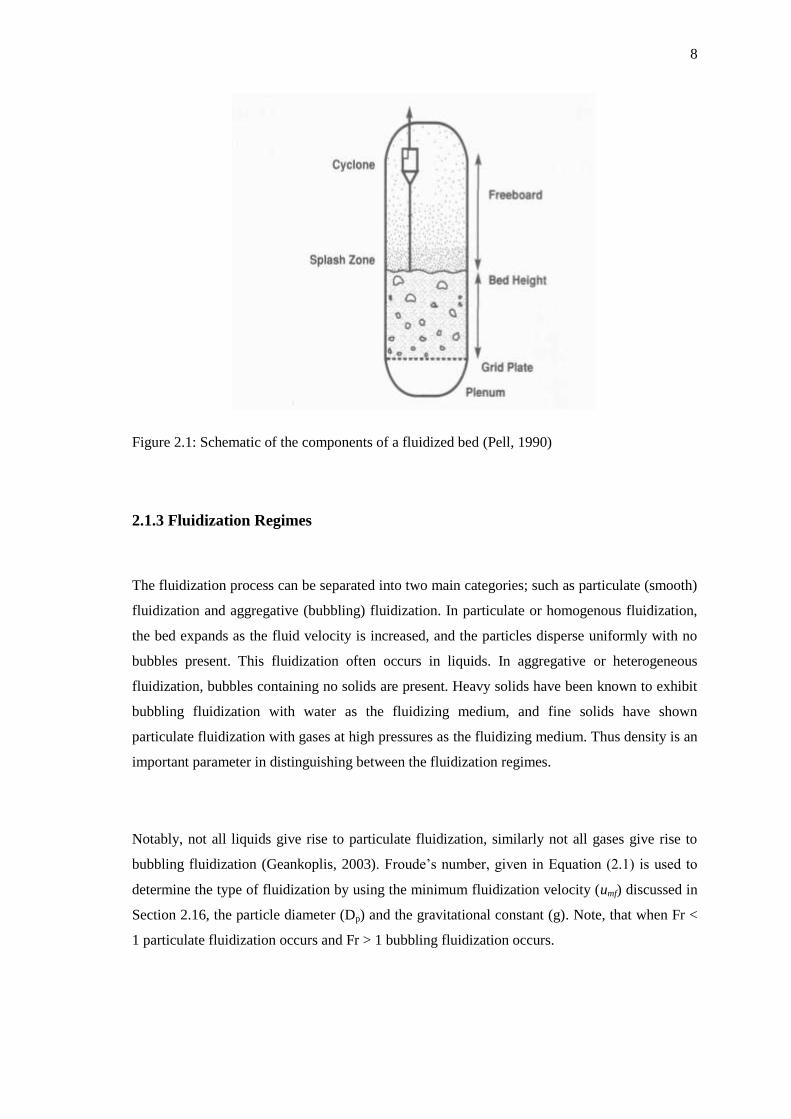
of a fluidized bed which are common throughout most types of designs. Figure 2.1 highlights

these main components which are; the plenum chamber, grid plate (distributor), bed height,

freeboard region, splash zone and the cyclone.

The plenum chamber is located below the gas distributor, which is where the fluidizing medium

first enters the bed. The gas distributor also referred to as the grid plate has a significant effect

on the proper operation of a fluidized bed (Pell, 1990). It is used to distribute the gas uniformly

7

into the fluidized bed to enable efficient gas-solids contacting. It also functions to support the

bed material, inhibit the back flow of solids and prevent the bed material from leaking into the

plenum chamber (Perry & Green, 1997). There are various designs for distributors, for example

pipe grid plates, straight-hole distributors and porous plates (Basu, 2006). These designs have a

substantial influence on the bed hydrodynamics and the rate of heat and mass transfer in the

fluidization process (Perry & Green, 1997).

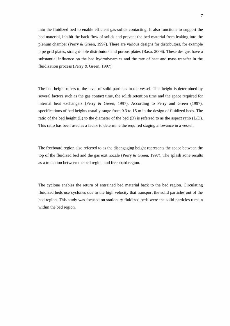
The bed height refers to the level of solid particles in the vessel. This height is determined by

several factors such as the gas contact time, the solids retention time and the space required for

internal heat exchangers (Perry & Green, 1997). According to Perry and Green (1997),

specifications of bed heights usually range from 0.3 to 15 m in the design of fluidized beds. The

ratio of the bed height (L) to the diameter of the bed (D) is referred to as the aspect ratio (L/D).

This ratio has been used as a factor to determine the required staging allowance in a vessel.

The freeboard region also referred to as the disengaging height represents the space between the

top of the fluidized bed and the gas exit nozzle (Perry & Green, 1997). The splash zone results

as a transition between the bed region and freeboard region.

The cyclone enables the return of entrained bed material back to the bed region. Circulating

fluidized beds use cyclones due to the high velocity that transport the solid particles out of the

bed region. This study was focused on stationary fluidized beds were the solid particles remain

within the bed region.

8

Figure 2.1: Schematic of the components of a fluidized bed (Pell, 1990)

2.1.3 Fluidization Regimes

The fluidization process can be separated into two main categories; such as particulate (smooth)

fluidization and aggregative (bubbling) fluidization. In particulate or homogenous fluidization,

the bed expands as the fluid velocity is increased, and the particles disperse uniformly with no

bubbles present. This fluidization often occurs in liquids. In aggregative or heterogeneous

fluidization, bubbles containing no solids are present. Heavy solids have been known to exhibit

bubbling fluidization with water as the fluidizing medium, and fine solids have shown

particulate fluidization with gases at high pressures as the fluidizing medium. Thus density is an

important parameter in distinguishing between the fluidization regimes.

Notably, not all liquids give rise to particulate fluidization, similarly not all gases give rise to

bubbling fluidization (Geankoplis, 2003). Froude‟s number, given in Equation (2.1) is used to

determine the type of fluidization by using the minimum fluidization velocity (umf) discussed in

Section 2.16, the particle diameter (Dp) and the gravitational constant (g). Note, that when Fr <

1 particulate fluidization occurs and Fr > 1 bubbling fluidization occurs.

9

(2.1)

This study was focused on gas-solid fluidized beds and the several regimes of fluidization that

exist within this system. The different types of fluidization regimes that occur are due to the

variation of parameters, such as the superficial gas velocity and the solid particle properties.

Figure 2.2 shows the different fluidization regimes of gas-solid fluidized beds based on

increasing superficial gas velocity.

A fixed bed regime also referred to as the static regime can be seen in Figure 2.2 A. This

fluidization regime is reached at very low superficial gas velocities. When the gas flows through

the bed it causes the solid particles to vibrate. However, the same bed height is maintained to

that of the bed at rest.

Figure 2.2 B depicts the minimum fluidization regime. This regime occurs when the drag force

conveyed by the superficial gas velocity equates to the weight of the solid particles in the bed.

The solid particles are transformed into a fluid-like state, which indicates the beginning of

fluidization. The bed voidage is also found to increase slightly. The superficial gas velocity at

which fluidization begins is referred to as the minimum fluidization velocity (umf).

The bubbling fluidization regime is observed in Figure 2.2 C. This regime occurs when an

increase in superficial gas velocity above the minimum fluidization velocity (umf) results in the

formation of bubbles. The gas passes through the bed as bubbles and little contact occurs

between the individual solid particles and the bubbles. High conversion of gaseous reactants or

high selectivity of a reaction intermediate cannot be achieved in this regime due to the

inefficient contacting (Kunii & Levenspiel, 1991). The superficial gas velocity at which the

bubbling fluidization regime begins is referred to as the minimum bubbling velocity (umb).

The bubbles will coalesce and grow as they rise up the fluidized bed column when the

superficial gas velocity is increased further. They can even grow to the entire cross section of a

column if the fluidized bed has a high aspect ratio i.e. a small diameter column with a deep bed

of solid particles. This occurrence is referred to as the slugging regime; seen in Figure 2.2 D.

10

This is an undesirable process in industry; due to the pressure fluctuations in the bed producing

substantial vibrations to the plant and also the increased entrainment of solid particles that

occur. Large diameters of commercial fluidized bed boilers or gasifiers have mitigated this issue

(Basu, 2006). The superficial gas velocity at which the slugging fluidization regime begins is

referred to as the minimum slugging velocity (ums).

The turbulent regime appears upon further increase of the superficial gas velocity beyond the

terminal velocity of the solid particles. This regime seen in Figure 2.2 E, and is classified by the

upper surface of the bed disappearing and a turbulent motion being observed. There is good gas-

solid contact within this regime. Reactor performances that have reached ideal back-mix reactor

approaches demonstrate the higher contact efficiency achieved in this regime (Basu, 2006).

The fast fluidization regime can be seen in Figure 2.2 F. This regime occurs when particles are

transported out of the bed and require replacing or recycling. This regime has a dense phase

region at the bottom of the vessel and a dilute phase region on the top with no visible bed

surface.

The pneumatic transport regime or pneumatic conveying can be seen in Figure 2.2 G. This

regime occurs with an increase in superficial gas velocity that results in solid particle

entrainment. The fluidized bed occurs in a disperse, dilute or lean phase.

This study was focused on gas-solid fluidized beds during aggregative fluidization represented

by the bubbling, slugging and turbulent regimes seen in Figure 2.2 C, D and E respectively.

11

Figure 2.2: Schematic of the different fluidization regimes that exist with increasing gas

velocity, adapted from Grace (1982)

2.1.4 Geldart Powder Classification

As mentioned in Section 2.1.3, the formation of the different types of fluidization regimes is due

to the variation of parameters, such as the solid particle properties. These properties refer to the

solid particle density and diameters for gas-solid fluidized bed systems. The type of material

used dictates the type of fluidization observed. This is due to the fact that not every particle can

be fluidized. Geldart (1973) classified the behaviour of solid particles that can be fluidized,

using gas as the fluidizing medium. Figure 2.3 shows this classification which is separated into

four main categories.

Group A particles are referred to as „aeratable‟. These particles have been classified with a small

mean particle size of 30 μm < dp < 100 μm and have a low density of ρp < 1400 kg/m3. They are

known to fluidize easily with smooth (particulate) fluidization occurring at low gas velocities,

and with no bubbles present. Upon increasing the superficial gas velocity above the minimum

fluidization velocity (umf), the bed is observed to expand quite significantly without the

formation of bubbles. Bubbles start forming at the minimum bubbling velocity (umb) which is

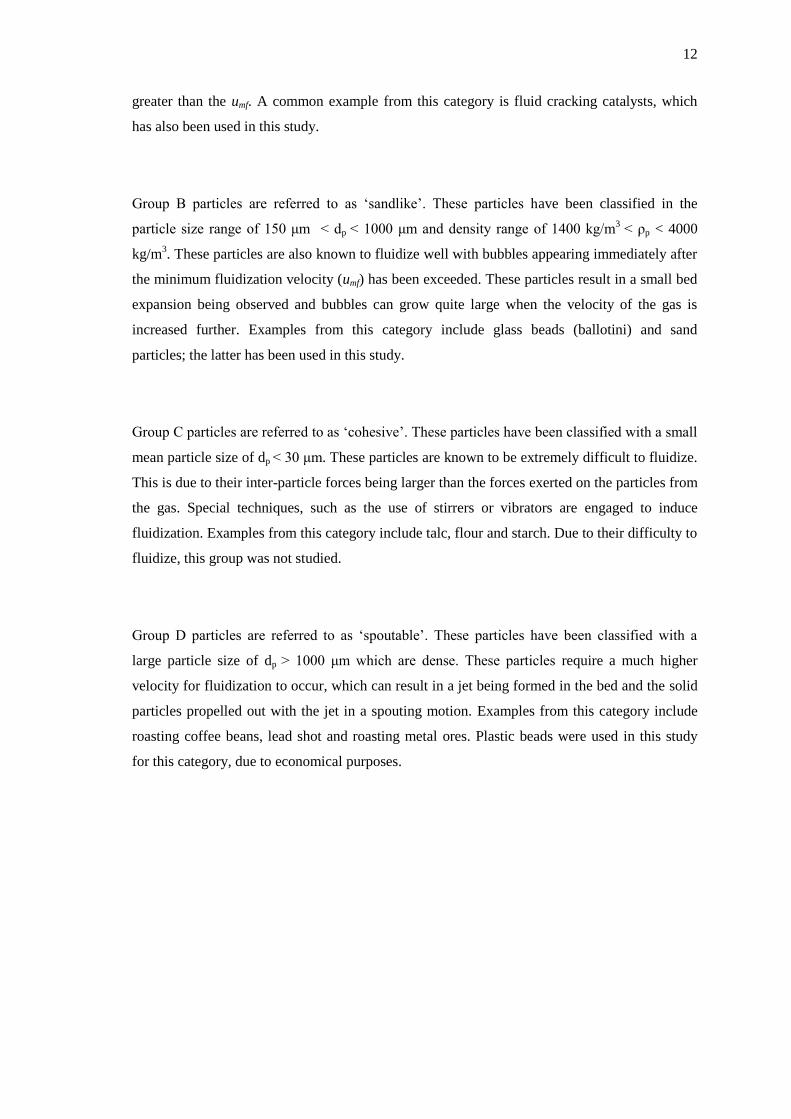
12

greater than the umf. A common example from this category is fluid cracking catalysts, which

has also been used in this study.

Group B particles are referred to as „sandlike‟. These particles have been classified in the

particle size range of 150 μm < dp < 1000 μm and density range of 1400 kg/m3

< ρp < 4000

kg/m3. These particles are also known to fluidize well with bubbles appearing immediately after

the minimum fluidization velocity (umf) has been exceeded. These particles result in a small bed

expansion being observed and bubbles can grow quite large when the velocity of the gas is

increased further. Examples from this category include glass beads (ballotini) and sand

particles; the latter has been used in this study.

Group C particles are referred to as „cohesive‟. These particles have been classified with a small

mean particle size of dp < 30 μm. These particles are known to be extremely difficult to fluidize.

This is due to their inter-particle forces being larger than the forces exerted on the particles from

the gas. Special techniques, such as the use of stirrers or vibrators are engaged to induce

fluidization. Examples from this category include talc, flour and starch. Due to their difficulty to

fluidize, this group was not studied.

Group D particles are referred to as „spoutable‟. These particles have been classified with a

large particle size of dp > 1000 μm which are dense. These particles require a much higher

velocity for fluidization to occur, which can result in a jet being formed in the bed and the solid

particles propelled out with the jet in a spouting motion. Examples from this category include

roasting coffee beans, lead shot and roasting metal ores. Plastic beads were used in this study

for this category, due to economical purposes.

13

Figure 2.3: Geldart classification of powders (Geldart, 1973)

2.1.5 Minimum Fluidization Voidage

The void fraction (ε) in a packed bed is defined by the volume of voids in the bed divided by the

total volume of the bed; which includes the volume of both voids and solids (Geankoplis, 2003).

The voidage of the bed when fluidization takes place is referred to as the minimum fluidization

voidage (εmf). The fluidized bed is known to expand to this voidage prior to the appearance of

particle motion.

This minimum voidage (εmf) has been studied extensively by many researchers for various

materials by determining the minimum fluidization bed height (Lmf). For the uniform cross-

sectional area, A and a volume, which is equal to the total volume of solids. A

relationship between the bed height, L and bed voidage, ε can be developed, which is seen in

Equation (2.3). Note that L1 is the height of bed with voidage ε1 and L2 is the height of bed with

voidage ε2 (Geankoplis, 2003).

(2.2)

14

(2.3)

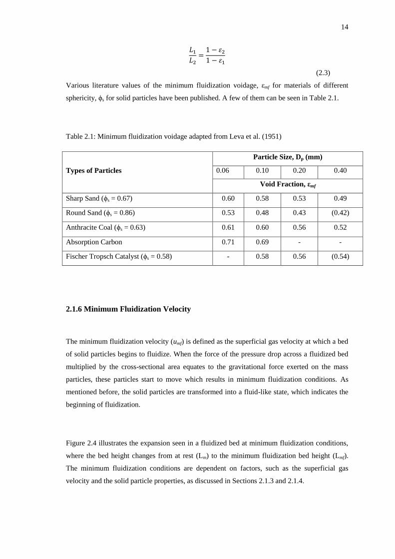
Various literature values of the minimum fluidization voidage, εmf for materials of different

sphericity, ϕs for solid particles have been published. A few of them can be seen in Table 2.1.

Table 2.1: Minimum fluidization voidage adapted from Leva et al. (1951)

Types of Particles

Particle Size, Dp (mm)

0.06 0.10 0.20 0.40

Void Fraction, εmf

Sharp Sand (ϕs = 0.67) 0.60 0.58 0.53 0.49

Round Sand (ϕs = 0.86) 0.53 0.48 0.43 (0.42)

Anthracite Coal (ϕs = 0.63) 0.61 0.60 0.56 0.52

Absorption Carbon 0.71 0.69 - -

Fischer Tropsch Catalyst (ϕs = 0.58) - 0.58 0.56 (0.54)

2.1.6 Minimum Fluidization Velocity

The minimum fluidization velocity (umf) is defined as the superficial gas velocity at which a bed

of solid particles begins to fluidize. When the force of the pressure drop across a fluidized bed

multiplied by the cross-sectional area equates to the gravitational force exerted on the mass

particles, these particles start to move which results in minimum fluidization conditions. As

mentioned before, the solid particles are transformed into a fluid-like state, which indicates the

beginning of fluidization.

Figure 2.4 illustrates the expansion seen in a fluidized bed at minimum fluidization conditions,

where the bed height changes from at rest (Lm) to the minimum fluidization bed height (Lmf).

The minimum fluidization conditions are dependent on factors, such as the superficial gas

velocity and the solid particle properties, as discussed in Sections 2.1.3 and 2.1.4.

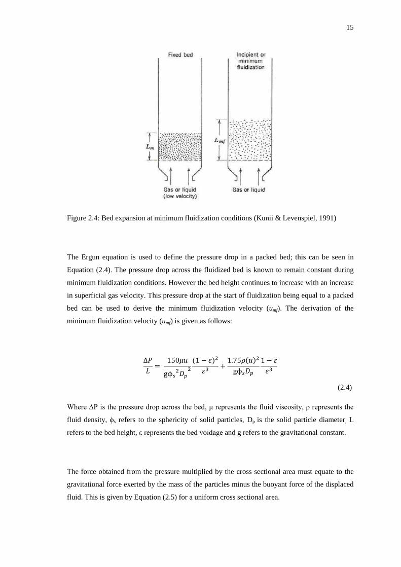
15

Figure 2.4: Bed expansion at minimum fluidization conditions (Kunii & Levenspiel, 1991)

The Ergun equation is used to define the pressure drop in a packed bed; this can be seen in

Equation (2.4). The pressure drop across the fluidized bed is known to remain constant during

minimum fluidization conditions. However the bed height continues to increase with an increase

in superficial gas velocity. This pressure drop at the start of fluidization being equal to a packed

bed can be used to derive the minimum fluidization velocity (umf). The derivation of the

minimum fluidization velocity (umf) is given as follows:

(2.4)

Where ∆P is the pressure drop across the bed, μ represents the fluid viscosity, ρ represents the

fluid density, ϕs refers to the sphericity of solid particles, Dp is the solid particle diameter, L

refers to the bed height, ε represents the bed voidage and g refers to the gravitational constant.

The force obtained from the pressure multiplied by the cross sectional area must equate to the

gravitational force exerted by the mass of the particles minus the buoyant force of the displaced

fluid. This is given by Equation (2.5) for a uniform cross sectional area.

16

( )( )

(2.5)

By substituting Equation (2.5) into Equation (2.4), this results in Equations (2.6) which is used

to determine the minimum fluidization velocity (umf).

( )

(2.6)

Further simplification of Equation (2.6) can be achieved with the use of dimensionless numbers.

Reynolds Number (Re) which is defined as the ratio of inertial forces to the viscous forces at

minimum fluidization conditions is given by Equation (2.7).

(2.7)

When substituting Re into Equation (2.6), a simplified Equation (2.8) results.

( )

(2.8)

Note that for small particles where Remf < 20 the first term in Equation (2.8) can be removed

and for large particles where Remf > 1000 the second term in Equation (2.8) can be removed

(Geankoplis, 2003).

Archimedes Number (Ar) which is defined as the ratio of the gravitational forces to the viscous

forces is seen in Equation (2.9).

( )

(2.9)

When substituting Ar into Equation (2.8), a further simplified Equation (2.10) results.

(2.10)

17

Equation (2.10) has been modified into Equation (2.11) by defining constants

and

. Several authors have developed values for these constants which can be seen in

Table 2.2. These correlations can be used to predict the minimum fluidization velocity (umf) by

manipulating Reynolds Number from Equation (2.7).

(2.11)

Table 2.2: Correlations to determine the minimum fluidization velocity

Author Equation

(Wen & Yu, 1966) [ ]

(Bourgeois & Grenier, 1968) [ ]

(Chitester et al., 1984) [ ]

(Reina, et al., 2000) [ ]

(Hilal, et al., 2001) [ ]

2.1.7 Minimum Bubbling Velocity

The minimum bubbling velocity (umb) is defined as the superficial gas velocity at which a bed of

solid particles begins to form bubbles. Group B and D particles are known to exhibit bubbling

fluidization reasonably close to the minimum fluidization velocity (umf). Group A particles do

not commence bubbling upon exceeding the minimum fluidization velocity (umf), only bed

expansion is observed. When the minimum bubbling velocity (umb) is significantly greater than

the minimum fluidization velocity (umf) only then do bubbles start to appear in the bed (Basu,

2006).

Geldart and Abrahamsen in 1978 developed an Equation (2.12) to determine the the miminum

bubbling velocity.

18

(

)

(2.12)

They went on to further develop another Equation (2.13) in 1980 for smaller particles with a

mass fraction (F) less than 45 μm, for Group A particles.

*

+

(2.13)

2.1.8 Minimum Slugging Velocity

The minimum slugging velocity (ums) is defined as the superficial gas velocity at which a bed of

solid particles begins to form slugs. Slugging is characterized by the size of bubbles close in

size to the diameter of the fluidized bed column. This is common for fluidized beds with a high

aspect ratio i.e. a small column diameter to deep bed height. Yang (1976) determined that the

criterion for slug formation was given by Equation (2.14)

(2.14)

Note that ut is the terminal velocity and D is the diameter of the fluidized bed column.

However, Geldart (1986) found that the condition for the formation of slugs was that the

maximum stable bubble size needed to be greater than 0.6 times the diameter of the fluidized

bed. Correlations to determine the minimum slugging velocity have been developed by several

authors seen in Table 2.3.

19

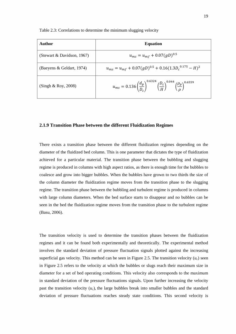
Table 2.3: Correlations to determine the minimum slugging velocity

Author Equation

(Stewart & Davidson, 1967)

(Baeyens & Geldart, 1974)

(Singh & Roy, 2008) (

)

(

)

(

)

2.1.9 Transition Phase between the different Fluidization Regimes

There exists a transition phase between the different fluidization regimes depending on the

diameter of the fluidized bed column. This is one parameter that dictates the type of fluidization

achieved for a particular material. The transition phase between the bubbling and slugging

regime is produced in columns with high aspect ratios, as there is enough time for the bubbles to

coalesce and grow into bigger bubbles. When the bubbles have grown to two thirds the size of

the column diameter the fluidization regime moves from the transition phase to the slugging

regime. The transition phase between the bubbling and turbulent regime is produced in columns

with large column diameters. When the bed surface starts to disappear and no bubbles can be

seen in the bed the fluidization regime moves from the transition phase to the turbulent regime

(Basu, 2006).

The transition velocity is used to determine the transition phases between the fluidization

regimes and it can be found both experimentally and theoretically. The experimental method

involves the standard deviation of pressure fluctuation signals plotted against the increasing

superficial gas velocity. This method can be seen in Figure 2.5. The transition velocity (uc) seen

in Figure 2.5 refers to the velocity at which the bubbles or slugs reach their maximum size in

diameter for a set of bed operating conditions. This velocity also corresponds to the maximum

in standard deviation of the pressure fluctuations signals. Upon further increasing the velocity

past the transition velocity (uc), the large bubbles break into smaller bubbles and the standard

deviation of pressure fluctuations reaches steady state conditions. This second velocity is

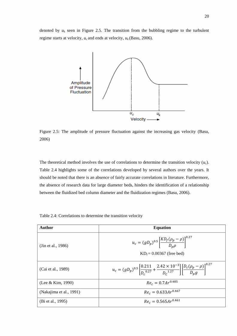
20

denoted by uk seen in Figure 2.5. The transition from the bubbling regime to the turbulent

regime starts at velocity, uc and ends at velocity, uk (Basu, 2006).

Figure 2.5: The amplitude of pressure fluctuation against the increasing gas velocity (Basu,

2006)

The theoretical method involves the use of correlations to determine the transition velocity (uc).

Table 2.4 highlights some of the correlations developed by several authors over the years. It

should be noted that there is an absence of fairly accurate correlations in literature. Furthermore,

the absence of research data for large diameter beds, hinders the identification of a relationship

between the fluidized bed column diameter and the fluidization regimes (Basu, 2006).

Table 2.4: Correlations to determine the transition velocity

Author Equation

(Jin et al., 1986)

*

+

KDf = 0.00367 (free bed)

(Cai et al., 1989) *

+ *

+

(Lee & Kim, 1990)

(Nakajima et al., 1991)

(Bi et al., 1995)

21

2.2 Methods for Analysis of Pressure Fluctuations

Over the years pressure fluctuation signals in fluidized beds have been used as a measure of

bubble intensity. These signals are used for the identification of various phenomena such as

agglomeration, formation, coalescence and eruption of bubbles (Davidson et al., 1985).

Pressure fluctuations have been found to be extremely influenced by variables, such as the

bubble size, bubbling rising velocity and the motion of the bed surface. These variables in turn

are related to the fluidization regimes within a fluidized bed (Fan et al., 1981).

Due to this relationship between the fluidization state and pressure fluctuations within the

fluidized bed; a method was developed to analyse the potential information inside a fluidized

bed column (Kage et al., 2000). The advantage of using pressure fluctuations is the ease of

operability when measuring pressure fluctuations in a fluidized bed, even under tough industrial

conditions. Other advantages include the inexpensive cost factor and its non-intrusive nature,

which inhibits any alteration of flow around the measurement point. These benefits have made it

one of the most common methods for fluidized beds studies (van Ommen et al., 2011). The

disadvantage however is that the interpretation and analysis of the pressure fluctuation signals is

not direct; therefore many researchers have been working on improving the understanding of

pressure fluctuations in fluidized beds.

The time-series analysis of the pressure fluctuation signals in fluidized beds is used to obtain a

quantitative description of the different fluidization regimes (van Ommen et al., 2011). Studies

have also shown that measurements of the signal symmetry can be used to identify the

transitions between the different fluidization regimes. The time-series analysis of pressure

fluctuation signals can be separated into three categories, such as the time domain analysis, the

frequency domain analysis and the state-space domain analysis (van Ommen et al., 2011).

2.2.1 Time Domain Analysis

The method of analysis in the time domain denotes the simplest approach for investigating

pressure fluctuation signals in a fluidized bed. The time domain analysis is used to generate a

depiction of the different fluidization regimes achieved from measurements of pressure

22

fluctuations signals inside the fluidized bed. This method illustrates the pressure fluctuation

signals against time for a particular fluidization regime. A representation, taken from Alberto et

al. (2004), of the technique can be seen in Figure 2.6 for the bubbling regime using sand

particles. A qualitative visualization of the complexity of the fluidization regime can be seen in

this method. This signal is usually inspected before further analysis. This is to ensure that

accurate data was obtained from the data acquisition system and that no irregularities in bed

behaviour have occurred (van Ommen et al., 2011).

Figure 2.6: Time-series of the bubbling regimes using sand with a 290 μm diameter in fluidized

bed column of 11.5 cm at a bed height of 11 cm (Alberto et al., 2004)

Standard deviation or variance (viz. second order statistical moment) attained from the

amplitude of pressure fluctuation signals is another commonly used time domain analysis

method. This method examines the relationship between the standard deviation from the

amplitude of pressure fluctuation signals against the superficial gas velocity. This technique

refers to the experimental method discussed in Section 2.1.9 and the representation of this

method was shown in Figure 2.5.

The standard deviation technique has the advantage of identifying a change in fluidization

regime, defining the minimum fluidization velocity and even detecting if defluidization has

occurred in industrial fluidized bed reactors (van Ommen et al., 2011). This method has also

23

been used as an on-line monitoring tool for the determination of particle size in fluidized bed

hydrodynamics (Davies et al., 2008). The standard deviation method has often been used to

define the transition velocity from the bubbling fluidization regime to the turbulent fluidization

regime (Bi et al., 2000). The maximum in standard deviation is represented by the transition

velocity (uc). This velocity denotes the beginning of the transition phase of the fluidization

regime.

However, Andreux et al. (2005) showed that the velocity at which the transition phase begins

might be over predicted by the standard deviation. Furthermore there is uncertainty for the

method to be applicable in industry. This is due to the dependence of the technique to the

superficial gas velocity, which is known to vary quite substantially in industry. The dynamics of

flow are highly influenced by the distribution of solid particles within the system. Therefore

this method needs to be applied with high accuracy for the standard deviation amplitude in

pressure fluctuations (van Ommen et al., 2011).

2.2.2 Frequency Domain Analysis

The method of analysis in the frequency domain denotes the most common approach for

investigating pressure fluctuation signals in a fluidized bed. Also referred to as power spectral

analysis, this method is used to quantify the different fluidization regimes achieved in gas-solid

fluidized bed systems. This technique depicts the amplitude of pressure fluctuation signals

against the dominant frequency for a particular fluidization regime. A representation, taken

from Alberto et al. (2004), of the method can be seen in Figure 2.7 for the bubbling regime

using sand particles. Analysis is achieved by examining the power spectra and uses the

dominant frequencies by associating it with the pressure fluctuations in the fluidized bed (van

Ommen et al., 2011). A dominant frequency is defined as the frequency with the highest peak.

24

Figure 2.7: Power spectra of the bubbling regime using sand with a 290 μm diameter in

fluidized bed column of 11.5 cm at a bed height of 11 cm (Alberto et al., 2004)

The Fast Fourier Transform (FFT) is a mathematical tool that is used to transform a signal from

a function of time to a signal from a function of frequency thus enabling the analysis in the

frequency domain. The derivation for the FFT is given below which has been adapted from

Alberto et al. (2004).

The Fourier Transform for a function x(t) in the finite time interval from 0 to T is defined by

Equation (2.15).

∫

(2.15)

Note that x(t) is the time domain signal, X(f) is the FFT and f is the frequency to analyse.

The time domain is sampled at N points that are equally spaced at a distance ∆t. The sampling

time is defined as but it is appropriate to begin with n = 0; which eventually results in

Equation (2.16).

(2.16)

25

Note that n = 0, 1, 2, 3…, N-1

Similarly for the frequency, the discrete form of Equation (2.15) is given by Equation (2.17):

∑ [ ]

(2.17)

The discrete values of frequency used to calculate X (f, T) is given by Equation (2.18):

(2.18)

Note that k = 0, 1, 2, 3…, N-1

The Fourier components of the transformed values are determined by:

∑ [

]

(2.19)

Note that k = 0, 1, 2, 3…, N-1

The FFT calculation is capable of processing the amounts of Xk that will appear to the larger or

smaller amplitude, which is in agreement with the characteristic of the process analysed

(Alberto et al., 2004).

The shape of the spectrum as well as the statistical consistency of data is determined by the

number of samples recorded. A minimum sampling frequency of 20 Hz is suitable for a

statistical consistency spectrum (Johnsson et al., 2000).

Johnsson et al. (2000) determined that when a transition between fluidization regimes occurred,

a clear change in frequency distribution with a much wider spectrum was observed. And if no

transition between fluidization regimes resulted then there was slight change in the frequency

distribution with an increase in superficial gas velocity. The dominant frequencies in the power

spectra arise in each fluidization regime due to the bubbles or slugs passing through the

fluidized bed.

26

Several researchers have found that fluidization regimes transitions are identified by the change

in frequency distribution in the power spectra. However the disadvantage in the analysis of this

method is that the interpretation and observation of the power spectra with the dominant

frequency is different for each researcher. Thus analysis in the frequency domain can also be

quite subjective. But it still remains a far more accurate and enhanced representation of the

fluidization regime compared to that of the time domain method.

Spectral analysis has also been used to validate scale up relationships of fluidized bed units, by

comparing spectra from a model to a full scale unit (Nicastro & Glicksman, 1984).

2.2.3 State Space Domain Analysis

The third method of analysis for investigating pressure fluctuation signals in a fluidized bed is

in the state space domain. This method is also referred to as the chaos analysis technique. This

method is used to supplement the time and frequency domain methods. However, it is most

commonly used in non-linear analysis, which is found in two-phase flow in fluidized bed

systems (van Ommen et al., 2011).

A state of a fluidized bed can be determined by projecting all variables governing the system

into a multi-dimensional space, otherwise referred to as the state space for a certain period of

time. An „attractor‟ is defined as a collection of these states of the system for the entire time

period (Johnsson et al., 2000). The state space domain technique uses the attractor as a basis for

the analysis of the pressure fluctuation signals. The attractor is unable to provide enough

information on its own and therefore characteristics have been developed to support the model.

These characteristics are used to determine the behaviour within a fluidized bed. They are

measured through the Lyapunov exponents, the Kolmogorov entropy and the correlation

dimension (van Ommen et al., 2011). The Lyapunov exponent and Kolmogorov entropy method

are used to measure the predictability of the system, as well as the sensitivity to the initial

conditions that were set. Whereas the correlation dimension method expresses the number of

degrees of freedom the system has (Johnsson et al., 2000).

27

The Kolmogorov entropy is the most common method for fluidized bed hydrodynamics

analysis. It uses the concept of two points on the attractor that are closer than the defined small

length scale. The entropy method is determined with a high level of accuracy when a large

number of pairs are used. The Lyapunov exponents use the local rate of either convergence or

divergence on two points of the attractor. The main disadvantage with this method is calculating

incorrect results, due to the dimension of the reconstructed state space being larger than the true

dimension of the state space (Johnsson et al., 2000).

These analysis techniques are not commonly employed in this study due to the dependence

factor on the calculation of certain parameters for each characteristic. Literature has deficiencies

in the extensive range of fluidization regimes by analysis in the state space domain.

2.3 Scale Up

Scale up is one of the most complex topics within fluidized bed technology. This is due to the

vast differences in the hydrodynamic state of beds in different aspect ratios (ratio of the bed

height and column diameter). For example, the hydrodynamics of gas-solid fluidized bed

systems and the contacting regimes are relatively different when comparing; a small diameter

fluidized bed with a high aspect ratio and a large diameter fluidized bed with a moderate aspect

ratio. This is evident when bubbles are small and cannot grow larger than the vessel diameter in

small diameter fluidized beds. However in larger fluidized bed columns which are also deep in

bed height, bubbles are able to grow very large. These large bubbles have less surface area for

mass transfer to the solids compared to the same volume of the small bubbles. It is also found

that the large bubbles rise through the bed more rapidly (Perry & Green, 1997). Therefore high

precision needs to be employed when implementing scale-up relationships for fluidized beds.

Basu (2006) showed that good scale-up in gas-solid fluidized bed systems involves a balance

among factors such as the combustion, heat transfer and hydrodynamic processes.

Horio et al. (1986) developed scaling relationships for bubbling fluidized beds. A scale factor,

m is determined by the ratio of the diameter, D of a fluidized bed in the model unit to a

diameter, D0 of a fluidized bed in a prototype unit.

28

(2.20)

For Geldart Group B particles which have a similar bubble fraction, bubble size distribution,

solids circulation and mixing; Equation (2.21) must be satisfied:

√ ( )

(2.21)

For Geldart Group A particles which have a similar bubble size distribution; Equation (2.22)

must be satisfied:

√

(2.22)

Note that for Equations (2.21) and (2.22) u and umf is the superficial gas velocity and minimum

fluidization velocity respectively for the model unit and u0 and umf

0 is the superficial gas

velocity and minimum fluidization velocity respectively for the prototype unit.

Glicksman et al. (1993) determined the following the non-dimensional parameter seen below for

particle shapes that are too different. This parameter ensures that the model and prototype

remain unchanged and keeps the particle size distribution similar.

29

3

CHAPTER THREE

3. EXPERIMENTAL EQUIPMENT

3.1 The Gas-Solid Fluidized Bed Apparatus

The experimental equipment composed of an existing laboratory-scale gas-solid fluidized bed

and data acquisition system at the School of Chemical Engineering of the University of

KwaZulu-Natal, which were used to conduct the required experimental work and analysis.

A schematic representation of the entire experimental setup is shown in Figure 3.1. The

experimental setup was designed for use of one of the three fluidized bed columns at a time. A

second schematic representation depicting a single fluidized bed column is shown in Figure 3.2.

Furthermore, only one pressure transmitter is shown on the diagrams. The pressure transmitters

were chosen based on the operating range required for fluidization; hence only one transmitter

was used at a time. The laboratory-scale gas-solid fluidized bed system used in this project

consisted of the apparatus seen in Figure 3.3.

30

Figure 3.1: Schematic representation of the entire experimental gas-solid fluidized bed system

A – Air inlet from compressor; B – Gate valve; C, D, E – Stop valves; F, G H – Rotameters; I – Pressure gauge; J - Fluidized Bed 1 (I.D 5 cm, Total

Height 200 cm); K - Fluidized Bed 2 (I.D 11 cm, Total Height 153 cm); L - Fluidized Bed 3 (I.D 29 cm, Total Height 507.5 cm); M, N, O – Solid

particles; P, Q, R – Plenum chamber

31

Figure 3.2: Schematic representation of the experimental gas-solid fluidized bed system

A – Air inlet from Compressor; B – Gate Valve ; C, D, E – Stop Valves ; F, G, H – Rotameters;

I – Plenum Chamber ; J – Pressure Measurement Point; K – Air Distributor; L – Solid Particles;

M – Fluidized Bed Column; N – Pressure Probe; O - Pressure Transmitter; P – Data

Acquisition Board; Q – Pressure Signal to Computer

32

Figure 3.3: Lab-scale gas-solid fluidized bed system

A – Rotameter 3; B – Rotameter 2; C – Rotameter 1; D – Fluidized Bed 1 (I.D 5 cm, Total

Height 200 cm); E - Fluidized Bed 2 (I.D 11 cm, Total Height 153 cm); F - Fluidized Bed 3

(I.D 29 cm, Total Height 507.5 cm); G – WIKA model P30 Pressure Transmitter (Range 0 – 1.6

bar abs.); H – WIKA model D-10-P Pressure transmitter (Range 0 – 20 bar rel.); I – WIKA

model 2500 Digital Pressure Gauge

The following equipment encompassed the gas-solid fluidized bed system:

Air Compressor

Air Distributor

Three Rotameters

Three Cylindrical Fluidized Beds constructed with Perspex

o Fluidized Bed 1 (I.D 5 cm, Total Height 200 cm)

o Fluidized Bed 2 (I.D 11 cm, Total Height 153 cm)

o Fluidized Bed 3 (I.D 29 cm, Total Height 507.5 cm)

WIKA model P30 Pressure Transmitter (Range 0 – 1.6 bar abs.)

WIKA model D-10-P Pressure Transmitter (Range 0 – 25 bar)

WIKA model 2500 Digital Pressure Gauge (Range 0 – 6 bar)

DC Power Supply

Data Acquisition System

A B C

H

I

D

F

E

G

33

3.1.1 Fluidized Bed

The main component of the apparatus is the cylindrical fluidized bed column. This represents

the unit in which fluidization of solid particles occurs upon contact with the fluidizing medium

(i.e. compressed air for this experiment). The edges of the column are smooth to reduce the wall

pressure drop and to hinder small particles such as dust collecting. Visual observation was vital

in qualitative classification of each fluidization regime. Therefore columns constructed of

Perspex, which are transparent, were chosen to conduct experiments. There were three fluidized

bed columns each with different column diameter and height as described above employed in

this study. Each column was used independently of one another with various materials and bed

height. Usually fluidized bed columns contain cyclones which enable the return of entrained

material to the bed, but since all three columns were adequately elevated this was not required.

3.1.2 Bed Height

As mentioned in Section 2.1.2, the bed region represents the section of the fluidized bed column

where solid particles are enclosed. Hence the bed height refers to the level of solids in the

column. Three different materials from each of Geldarts classification of fluidized particles

(Group A – spent FCC; Group B – sand and Group D – plastic beads) were employed in each

fluidized column at different bed heights. The bed height was determined by factors such as

gas-contact time and the ratio of the bed height (L) to the diameter of the bed (D); referred to as

the aspect (L/D) ratio.

3.1.3 Distributor

As mentioned in Section 2.1.2, the gas distributor has a significant influence on the proper

operation of a fluidized bed. Its main function is to uniformly distribute gas into the bed, thus

initiating effective gas-solids contacting. All three fluidized bed columns had a perforated plate

with 1 mm holes as the distributor; which corresponded to the work from Alberto et al. (2004).

The position of the perforated distributor plate for each fluidized bed column is given as

follows:

34

Fluidized Bed 1 (I.D 5 cm) – 15 cm above the column base



3.1.4 Plenum Chamber

As mentioned in Section 2.1.2, the plenum chamber represents the area of the fluidized bed that

is positioned directly below the distributor plate. Air which is the fluidizing medium for this

study was allowed to enter the plenum chamber at the bottom through the main air supply

system. It contains packing material which was used for even distribution of the air flow into

the fluidized bed. Also located on the plenum chamber were pressure measurement points for all

three fluidized beds.

3.1.5 Flow Measurement and Control

The fluidizing gas velocity was provided by a 6 bar compressed air supply, feeding to a set of

three rotameters. A gate valve was used to control the flow into the fluidized bed. The three

rotameters consisted of three different sizes ranging from small, medium and large. The choice

of rotameter used during experiments was influenced by the size of each fluidized bed column.

The rotameters were calibrated at room temperature and 140 kPa. The calibration equations to

obtain the gas flow rate in L/min are as follows:

Note that R represents the rotameter reading

35

3.1.6 Pressure Measurement and Control

The pressure transmitter was used to record pressure fluctuations at a point on the fluidized bed

column by connecting a pressure probe from the transmitter to the measuring point for each of

the three fluidized beds. The pressure probe was constructed from polyethylene tubes with an

internal diameter of 3 mm. According to van Ommen et al. (2000) the length of each segment of

polyethylene tube had to be shorter than 60 cm for accurate readings; this was implemented for

experiments. The measurement point is usually chosen to be at the centre of the bed since the

fluidization regimes are completely developed at this location. However in order to ensure

accurate results the pressure probe had to be located in a region where it was not affected by

obstruction by fine particles which could result in damaging the pressure transmitter. The

location for measurements is vital to obtain accurate results and thus the plenum chamber was

chosen for the measuring points in each of the three fluidized bed columns. The pressure

measurement point in the plenum chamber for each fluidized bed column was as follows:

Fluidized Bed 1 (I.D 5 cm) – 3 cm below the distributor plate

Fluidized Bed 2 (I.D 11 cm) – 3.5 cm below the distributor plate

Fluidized Bed 3 (I.D 29 cm) – 3.5 cm below the distributor plate

The type of pressure transmitters used were the WIKA model P30 pressure transmitter which

ranged from zero to 1.6 bar absolute pressure and the WIKA model D-10-P pressure transmitter

which ranged from zero to 25 bar gauge pressure. The pressure measurement precision was

estimated at ± 0.05%. The WIKA model 2500 digital pressure gauge was used to determine the

minimum and maximum pressure fluctuations in the fluidization columns as well as verify the

measurements provided by the WIKA model P30 pressure transmitter and the WIKA model D-

10-P pressure transmitter.

A description of the software and data acquisition process can be found in the Easy Com 2011

Windows software manual.

36

3.2 Particle Size Analysis Equipment

To calculate the particle sizes for each of the three materials (spent FCC, sand and plastic beads)

different equipment was used to accommodate the various sizes of each material. For Geldart

Group A particles (spent FCC), a Shimadzu SALD-3101 laser diffraction particle size analyser

was used to determine the particle size; this equipment can be seen in Figure 3.4. Geldart Group

B particles (sand) could not be employed in the laser diffraction particle size analyser due to the

large size of the sand particles. Thus a vibrating screen shaker with varying size sieves was used

to determine the particle size; this equipment can be seen in Figure 3.5. And finally for Geldart

Group D particles (plastic beads) a digital calliper was used to determine the particle size. A

detailed description of the methods used to determine each particle size can be seen in Section

4.1.2.2.

Figure 3.4: Shimadzu SALD-3101 laser diffraction particle size analyser used to measure

Geldart Group A particles (spent FCC)

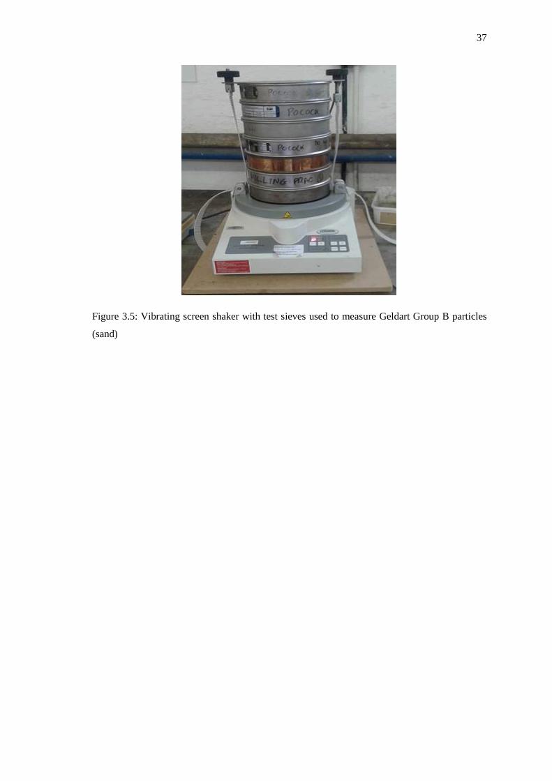
37

Figure 3.5: Vibrating screen shaker with test sieves used to measure Geldart Group B particles

(sand)

38

4

CHAPTER FOUR

4. EXPERIMENTAL METHODS

4.1 Particle Selection and Characterization

4.1.1 Particle Selection

Geldarts powder classification was used to determine the type of material required for

fluidization during this study as described in Section 2.4. For Group A particles, fluid cracking

catalysts is the most common material from this category, thus spent FCC was chosen. For

Group B particles, sand particles were chosen due to the low cost and being readily available in

laboratories. They fluidize well, and bubbles appear as soon as the minimum fluidization

velocity is exceeded. For Group D particles, plastic beads were chosen as the material to

emulate the spouting behaviour of this group. Large particles are known to cause instability and

result in slugging (Perry & Green, 1997). Group C is considered extremely difficult to fluidize

due to the large inter-particle forces compared to those resulting from action of the gas velocity

and therefore no experiments were undertaken for this category. In summary three different

materials from the different Geldart Groups were studied in this research.

Geldart Group A – spent FCC

Geldart Group B – Sand

Geldart Group D – Plastic Beads

4.1.2 Particle Characterization

Particle characterization tests include size distribution, density, voidage and sphericity. Tests

were conducted in the laboratory to determine the size and density of the specified materials

39

discussed in Section 4.1.1 for gas-solid fluidization. Particle size and density measurements

were conducted three times and the average has been represented in Table 4.1.

4.1.2.1 Particle Density

The liquid displacement test method was used to determine the density of the three materials

through use of a graduated cylinder. The density of spent FCC and sand was measured through

the use of water as the liquid medium and the density of the plastic beads was measured through

the use of 1-butanol as the liquid medium. The latter was due to the floating capacity of the

plastic beads in water and thus the margin of error was reduced due to an alcohol being used.

Lighter alcohols such as methanol, ethanol and 1-propanol were not utilized due to their high

volatility. The displacement method requires high accuracy of mass and volume measurements.

A digital mass balance with accuracy of ± 0.01 g was used for mass measurements. The

procedure to calculate the density of particles is given below:

The empty graduated cylinder was measured and defined as,

A sample of one of the particles (spent FCC or sand or plastic beads) was filled in the

graduated cylinder and measured and defined as,

The liquid either water or alcohol depending on the type of particle was filled up to the

line on the graduated cylinder and measured and defined as,

The mass of the liquid was calculated using, and the mass of solid

particles was calculated using, .

The volume of the liquid was calculated using,

; where density ρL is taken at

the temperature of the liquid. Note that the temperature measurements were conducted

using a mercury thermometer.

The volume of the solids was calculated using, .

And finally the particle density was calculated using,

.

40

4.1.2.2 Particle Size

To calculate the particle sizes for each of the three materials (spent FCC, sand and plastic beads)

different methods were employed to accommodate the various sizes of each particle. For

Geldart Group A particles (spent FCC), a Shimadzu SALD-3101 laser diffraction particle size

analyser seen in Figure 3.4 was used. This method exposes the solid particles to a laser light

with the particle size distribution determined from the light intensity distribution pattern of the

diffracted light emitted from the particles. The particle size is directly proportional to the light

intensity of diffracted light. The Shimadzu SALD-3101 laser diffraction particle size analyser

was only capable of measuring particles over a small range of diameters. The maximum size for

dry analysis is 300 μm. Therefore alternate methods of measuring the size distribution for the

remaining two materials were investigated.

In order to obtain the size distribution of sand particles (Group B), screening took place. This

was done in a 2 series of test sieves, ranging from 600 to 250 μm. The screening was done in a

vibrating screen shaker seen in Figure 3.5. For Geldart Group D particles (plastic beads), a

digital calliper was used to determine the size. The average was taken for a sample 20 beads at a

time.

For each particle size analysis, tests were conducted three times and the average was

represented. A summary of the particle characteristics conducted in this research can be seen in

Table 4.1 below.

Table 4.1: Particle characteristics of solid particles for gas-solid fluidization

Type of Material Particle Density

ρ (kg/m3)

Particle Size

(μm) Geldart Group

Spent FCC 1300 87 A

Sand 2600 300 B

Plastic Beads 830 4600 D

41

4.2 Preparation of the Gas-Solid System Equipment

4.2.1 Changing of Material

Proper change out of material was conducted in each fluidized bed column; to prevent

contamination, impurities and dust particles that could lead to inaccurate results. A high

pressure spray was used to clean out each column before the entry of a new product into the

column. This also improved the transparency of the column which ensured proper visualization

of each fluidization regime.

4.2.2 Back Flow of Material

The distributor which is designed to prevent back flow of solids during operation was carefully

monitored before each run. If the bed material were to leak into the plenum chamber this would

result in damage to the pressure transmitter due to particles entering the pressure probe via the

measurement point in the plenum chamber. The plenum chamber was transparent for all three

fluidized bed columns and thus the determination of back flow of solids could be easily

identified. For sand (Group B) and plastic beads (Group D), no back flow was observed.

Although, for spent FCC (Group A) due to the size of the particles it was observed to move

through to the plenum chamber slightly.

4.3 Operation of the Gas-Solid System Equipment

All experiments were conducted at ambient conditions. Each experiment was conducted in one

fluidized bed column at a time, which had one material and specified bed height under

investigation. The pressure transmitter was connected to the pressure measurement point and the

data acquisition board. The air supply was opened to allow the compressed air into the system.

Then the appropriate rotameter was selected for adjusting the air flow into the fluidized bed.

The pressure gauge for the rotameters had to be kept constant at 140 kPa, as they were

calibrated at this pressure. Visual observation was used to determine the fluidization regime.

Once the regime was found the pressure measurements were recorded on the software, Easy

42

Com 2011 Windows for each regime. The sampling frequency was specified as 500 Hz for the

WIKA P30 pressure transmitter; which corresponds to a sampling time of 2 ms. The total

experimental run time was set at 30 minutes. This procedure was repeated three times for

accuracy and for a new increasing rotameter reading until a new regime was reached.

The volumetric flow rate of air, Q was calculated using the selected rotameter calibration

equation. The cross sectional area of the fluidized bed was taken to be a cylinder and then

calculated using the respective column diameter;

. The superficial air velocity was

then calculated using,

. A summary of the operational conditions used during experiments

can be seen in Table 4.2 below.

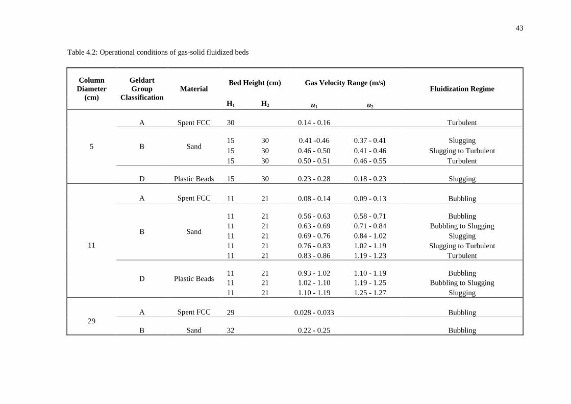
43

Table 4.2: Operational conditions of gas-solid fluidized beds

Column

Diameter

(cm)

Geldart

Group

Classification

Material Bed Height (cm) Gas Velocity Range (m/s)

Fluidization Regime

H1 H2 u1 u2

5

A Spent FCC 30

0.14 - 0.16

Turbulent

B Sand

15 30 0.41 -0.46 0.37 - 0.41 Slugging

15 30 0.46 - 0.50 0.41 - 0.46 Slugging to Turbulent

15 30 0.50 - 0.51 0.46 - 0.55 Turbulent

D

Plastic Beads

15 30 0.23 - 0.28 0.18 - 0.23 Slugging

11

A Spent FCC 11 21 0.08 - 0.14 0.09 - 0.13 Bubbling

B Sand

11 21 0.56 - 0.63 0.58 - 0.71 Bubbling

11 21 0.63 - 0.69 0.71 - 0.84 Bubbling to Slugging

11 21 0.69 - 0.76 0.84 - 1.02 Slugging

11 21 0.76 - 0.83 1.02 - 1.19 Slugging to Turbulent

11 21 0.83 - 0.86 1.19 - 1.23 Turbulent

D Plastic Beads

11 21 0.93 - 1.02 1.10 - 1.19 Bubbling

11 21 1.02 - 1.10 1.19 - 1.25 Bubbling to Slugging

11 21 1.10 - 1.19 1.25 - 1.27 Slugging

29

A Spent FCC 29

0.028 - 0.033

Bubbling

B

Sand 32

0.22 - 0.25

Bubbling

44

4.4 Measuring and Processing of Pressure Fluctuation Signals

To prevent any pitfalls during measuring of pressure fluctuations signals certain factors were

taken into account. The internal diameter of the pressure probe was kept to 2 mm as

recommended by van Ommen and Mudde (2007). This is due to smaller diameters which lead

to dampening of the signal and larger probe diameters increasing the resonance effects and

disturbing the local hydrodynamics. The time-series length of 30 minutes for spectral analysis

was used to be able to derive statistically sound results from the measurements as recommended

by van Ommen and Mudde (2007).

For consistent data the number of data points captured by the data acquisition is essential to

developing a broad spectrum. The time sampling was chosen at 30 min; which is in accordance

with van Ommen et al. (2011). Three runs were done per superficial gas velocity obtained for

each fluidization regime; this was to ensure higher accuracy of data. The experimental data was

analysed by dividing each of the three runs per regime into eight data segments comprising of

6000 data points. This ensures high precision of pressure signals with very little to no random

noise present. The Fast Fourier Transform (FFT) of each segment was then calculated through

MATLAB, which has a built in function that calculates the FFT. These results are then exported

to Microsoft Excel and sorted to determine the dominant frequency for each data segment. An

average dominant frequency was then taken over the three runs and shown in Chapter 5; the

results section of the study.

45

5

CHAPTER FIVE

5. RESULTS AND DISCUSSION

5.1 Experimental Observations

Experiments were conducted in three fluidized bed columns each with varying internal column

diameter (I.D) referred to as fluidized bed 1 (I.D of 5 cm), fluidized bed 2 (I.D of 11 cm) and

fluidized bed 3 (I.D of 29 cm). Visual observation of the various fluidization regimes was a vital

part to this study thus all fluidized bed columns utilized for experiments were constructed from

Perspex; which is a transparent material.

Geldart classification of powders for fluidization was used to determine the materials to conduct

experiments. For Geldart Group A materials, spent fluid catalytic cracking (FCC) was chosen. It

was found that spent FCC would stick to the side of the column after fluidization due to the

electrostatic charge forces present. This problem was mitigated with humid air to ensure

accurate results. For Geldart Group B materials, silica sand was chosen as it fluidizes well and

proved to be the only material that produced all fluidization regimes. Geldart Group D

materials, plastic beads were chosen to display the spouting behaviour. Large plastic beads to

the size of 4.6 mm were selected due to the quantity available for analysis in the large fluidized

bed column.

Three rotameters were used to control the amount of air flow into the gas-solid fluidized bed

system; which were calibrated at 140 kPa. Accurate data resulted from the maintenance of this

pressure using the pressure gauge on the system. The level was found to fluctuate at higher

velocities, during the turbulent regime for sand and slugging regime for plastic beads.

46

According to Davidson et al. (1985), pressure measurements must be located at the centre of the

bed. This was due to the fully developed state of fluidization occurring at this location, which

results in the most accurate data. Tests were conducted at different pressure measurement points

along the column for plastic beads. However, these results yielded very low pressure readings

compared to the actual pressure reading from the WIKA model 2500 digital pressure gauge.

Tests were not conducted for spent FCC and sand due to the risk of damaging the pressure

transmitter by penetration of fine particles, which was observed during normal operation. The

pressure measurement point was located at the plenum chamber for all three fluidized bed

columns; to prevent the obstruction of particles around the measuring point. Alberto et al.

(2004) recommended plenum chamber measurements for absolute pressure measurements.

Two bed heights were chosen for each fluidized bed column, the first height was the minimum

height which corresponded to the diameter of the respective column and the second height

equated to double the minimum height to demonstrate the effects of the ratio of the bed height

(L) to the diameter of the bed (D); referred to as the aspect (L/D) ratio. The different bed heights

for each fluidized bed column can be seen in Table 4.2.

It was observed for all fluidized bed columns that an increase of almost 2 cm in bed height

occurs at rest after fluidization was conducted in the column; i.e. the bed does not return to the

original bed height before fluidization. Also observed on all columns at increased bed heights,

was that each regime became more visible; for example there was no confusion between the

bubbling and slugging regimes. It was also noted that pressure fluctuation signals at elevated

bed heights display a higher pressure reading; as expected since there was more material to

fluidize and hence the force was greater.

5.2 Analysis in the Time Domain

5.2.1 Time-Pressure Analysis

Time domain analysis is accomplished by plotting a sequence of data points of a measured

signal, which in this study was a series of pressure fluctuation measurements as a function of

time. The advantage of examining the time pressure signal was to identify the irregularities in

the fluidized bed behaviour and inconsistencies with the data acquisition system. The visual

47

representation of the time pressure signal indicates the relevant time scale as well as the

complexity of the flow (van Ommen et al., 2011). The pressure fluctuation signals obtained

against time were analysed for consistent and periodic oscillations for each specific fluidization

regime. From these graphs, no irregularities in bed behaviour were noted (van Ommen et al.,

2011), thus confirming the credibility of the data received from the data acquisition system.

This also supported precise spectral analysis, as the pressure fluctuation signal was converted

into the frequency domain by use of the Fast Fourier Transform (FFT).

The results for sand in fluidized bed 2 are presented in this section due to the visual illustration

of all three fluidization regimes; bubbling, slugging and the turbulent regime occurring in this

column only. The results for materials spent FCC and plastic beads can be seen in Appendix A.

Visual identification was used to determine each fluidization regime by increasing the

superficial gas velocity of air into the fluidized bed column. As discussed in Section 2.1.3, the

bubbling regime was identified by the formation of bubbles that exploded at the bed surface.

The slugging regime was identified by the formation of large bubbles close in size to the

diameter of the column under study. And the turbulent regime was identified by the rapid

motion of solid clusters and the disappearance of the upper surface of the bed. Once each

fluidization regime was identified it was then possible to determine the transition regimes i.e.

the transition between the bubbling regime and slugging regime and the transition between the

slugging regime and turbulent regime.

Figure 5.1 and Figure 5.2 shows all regimes occurring for sand at bed heights of 11 cm and 21

cm respectively. It was observed that both the bubbling and slugging regimes resemble a similar

periodicity of the signal pattern with the slugging regime having slightly greater amplitude. Due

to the larger bubbles or slugs present in the slugging regime it would have been expected to

have a higher amplitude. The turbulent regime displayed the largest pressure fluctuation signal

due to the dynamic mixing of sand particles that occurred. At the elevated bed height of 21 cm,

it was observed that the pressure fluctuations for all three regimes behaved in the same manner

as the lower bed height (11 cm), with a greater amplitude. This was due to more bubbles

produced during the bubbling regime, more slugs produced at the slugging regime, and more

separation occurring at the turbulent regimes at the increased bed height. Since only amplitude

and signal variation profile parameters are used to distinguish between the different regimes, the

time domain analysis remains a subjective method. To avoid confusion between the fluidization

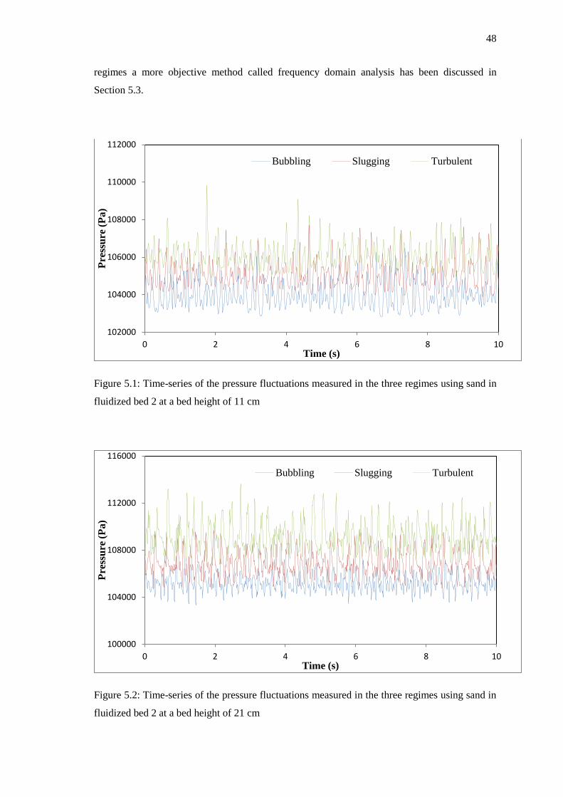
48

regimes a more objective method called frequency domain analysis has been discussed in

Section 5.3.


fluidized bed 2 at a bed height of 11 cm


fluidized bed 2 at a bed height of 21 cm

102000

104000

106000

108000

110000

112000

0 2 4 6 8 10

Pre

ssu

re (

Pa

)

Time (s)

Bubbling Slugging Turbulent

100000

104000

108000

112000

116000

0 2 4 6 8 10

Pre

ssu

re (

Pa)

Time (s)

Bubbling Slugging Turbulent

49

5.2.2 Predicted Minimum Fluidization Regime Velocity

The minimum fluidization velocity, umf is defined as the superficial gas velocity at which a bed

of solid particles begins to fluidize. As discussed in Section 2.1.6 several correlations have been

developed over the years to determine the umf. The results for umf found from the correlations

developed by the authors from Table 2.2 can be found in Table 5.1. These correlations are only

applicable for certain conditions and have a significant error of approximately 30% according to

Yang (2003).

For the small spent FCC particles and the large plastic beads particles the correlation results do

not compare with the experimental results due the vast size distribution of these particles.

According to Grace (1982) the kinetic energy term is negligible for small particles and

dominant for large particles. Therefore the constants C1 and C2 need to be modified in the

different umf correlations to account for this factor. However, limited research has been

developed for the different constant values to account for the different particle sizes.

For sand particles, the correlation results from Table 5.1 were overestimated for both fluidized

bed 1 and 2 when compared to the experimental data from Table 4.2. Fluidized bed 3 does not

compare, which could be due to the distributor on this column not distributing the gas uniformly

into the fluidized bed. This was observed from the bubbles only appearing at certain sections of

this column.

Table 5.1: Predicted results for the minimum fluidization velocity

Author

Minimum Fluidization Velocity

umf FCC

(m/s)

umf Sand

(m/s)

umf Plastic

Beads

(m/s)

(Wen & Yu, 1966) 0.0032 1.73 1.12

(Bourgeois & Grenier, 1968) 0.0040 1.37 1.08

(Chitester et al., 1984) 0.0046 1.52 1.23

(Reina et al., 2000) 0.0025 2.42 1.18

(Hilal et al., 2001) 0.0053 0.76 0.90

50

The minimum bubbling velocity, umb is defined as the superficial gas velocity at which bubbles

are first observed. As discussed in Section 2.1.7, Geldart and Abrahamsen (1978) developed an

equation (2.12) to determine the umb. However, the results only compared well for plastic beads;

the predicted umb at 0.89 m/s was very close to the experimental result of 0.91 m/s. It was noted

that for sand and plastic beads particles, upon further increase in gas flow exceeding the

respective columns umf bubbles started to form in the columns. This behaviour is typical of

Geldart Group B and Group D. However, spent FCC required an increase in superficial gas

velocity beyond the umb in order for bubbling to occur, which was characteristic of Geldart

Group A materials.

The minimum slugging velocity, ums is defined as the superficial gas velocity at which slugs or

bubbles close to the size of the column diameter are first observed. As discussed in Section

2.1.8, several authors have developed correlations to determine the ums as seen in Table 2.3. The

same equations used to determine the umf in Table 5.1 were used for the correlations to predict

the ums therefore it was expected that the results would be overestimated as well.

Stewart and Davidson (1967) developed an equation to determine the ums using the column

diameter and the umf, the results can be seen in Table 5.2. For spent FCC no slugging occurred in

any of the columns, typical of Geldart Group A material and therefore the results are not shown.

The sand results were overestimated for both fluidized bed 1 and 2. For plastic beads the

predicted results compared well for fluidized bed 2 but not fluidized bed 1. Slugging did not

occur in fluidized bed 3 for all materials due to the capacity of the compressor.

Baeyens and Geldart (1974) also developed an equation in addition to the Stewart and Davidson

(1967) equation to include the bed height to determine the ums, the results can be seen in Table

5.3. Only the results for fluidized bed 2 compared well for both materials, sand and plastic

beads. Once more the model did not compare well for fluidized bed 1. This could be due to the

small size of fluidized bed 1 and the subsequent difficulty in predicting the hydrodynamics

within a smaller vessel.

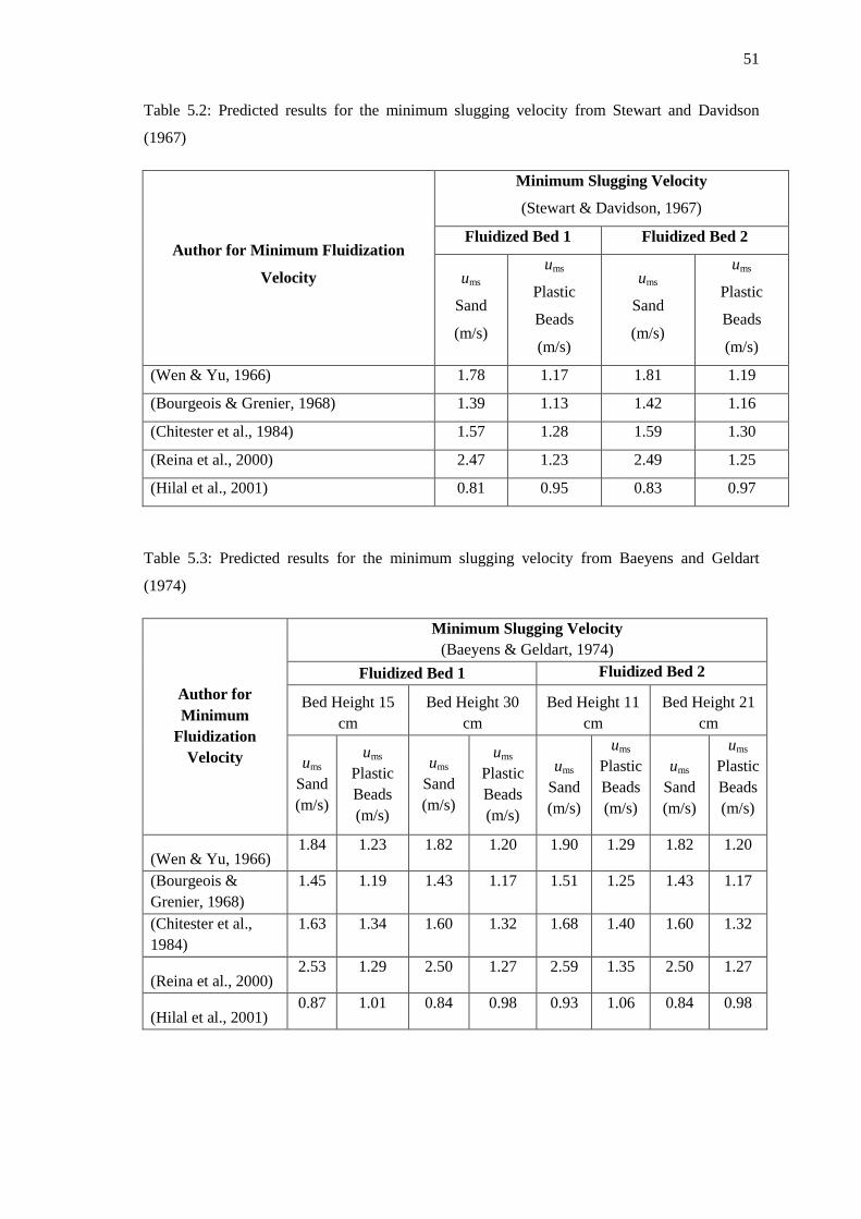
51

Table 5.2: Predicted results for the minimum slugging velocity from Stewart and Davidson

(1967)

Author for Minimum Fluidization

Velocity

Minimum Slugging Velocity

(Stewart & Davidson, 1967)

Fluidized Bed 1 Fluidized Bed 2

ums

Sand

(m/s)

ums

Plastic

Beads

(m/s)

ums

Sand

(m/s)

ums

Plastic

Beads

(m/s)

(Wen & Yu, 1966) 1.78 1.17 1.81 1.19

(Bourgeois & Grenier, 1968) 1.39 1.13 1.42 1.16

(Chitester et al., 1984) 1.57 1.28 1.59 1.30

(Reina et al., 2000) 2.47 1.23 2.49 1.25

(Hilal et al., 2001) 0.81 0.95 0.83 0.97

Table 5.3: Predicted results for the minimum slugging velocity from Baeyens and Geldart

(1974)

Author for

Minimum

Fluidization

Velocity


(Baeyens & Geldart, 1974)

Fluidized Bed 1 Fluidized Bed 2

Bed Height 15

cm

Bed Height 30

cm

Bed Height 11

cm

Bed Height 21

cm

ums

Sand

(m/s)

ums

Plastic

Beads

(m/s)

ums

Sand

(m/s)

ums

Plastic

Beads

(m/s)

ums

Sand

(m/s)

ums

Plastic

Beads

(m/s)

ums

Sand

(m/s)

ums

Plastic

Beads

(m/s)

(Wen & Yu, 1966) 1.84 1.23 1.82 1.20 1.90 1.29 1.82 1.20

(Bourgeois &

Grenier, 1968)

1.45 1.19 1.43 1.17 1.51 1.25 1.43 1.17

(Chitester et al.,

1984)

1.63 1.34 1.60 1.32 1.68 1.40 1.60 1.32

(Reina et al., 2000) 2.53 1.29 2.50 1.27 2.59 1.35 2.50 1.27

(Hilal et al., 2001) 0.87 1.01 0.84 0.98 0.93 1.06 0.84 0.98

52

The most recent correlation from Singh and Roy (2008) does not take into account the umf from

the various authors seen in Table 5.1, the results can be seen in Table 5.4. For sand it was found

that fluidized bed 1 did not compare well at both bed heights and was overestimated for

fluidized bed 2. No slugging occurred for sand in fluidized bed 3 but considering that the

experimental bubbling range was 0.22 to 0.25 m/s and the predicted value of ums was 0.27 m/s;

it can be concluded that the Stewart and Davidson (1967) and Baeyens & Geldart (1974) models

are more reliable at predicting the ums. For plastic beads the model did not predict well for

fluidized bed 1 but for fluidized bed 2 it compared very well.

Table 5.4: Predicted results for the minimum slugging velocity from Singh and Roy (2008)


(Singh & Roy, 2008)

Bed Heights

H1 H2 H1 H2

ums Sand

(m/s)

ums Plastic Beads

(m/s)

Fluidized Bed 1 0.78 0.75 2.06 2.00

Fluidized Bed 2 0.49 0.48 1.31 1.28

5.2.3 Predicted and Experimental Fluidization Regime Transition Velocity

The transition velocity from the bubbling to the turbulent regime as discussed in Section 2.1.9 is

defined as uc. Several correlations shown in Table 2.4 have been developed to determine this

velocity; the results can be seen in Table 5.5. For spent FCC, fluidized bed 1 was the only

column in which turbulent fluidization occurred however no change from the bubbling to

turbulent regime was observed to determine a transition velocity experimentally. The turbulent

regime velocity ranged from 0.14 to 0.16 m/s and none of the predicted values compared.

For plastic beads, the turbulent regime was not found in any column and the slugging regime

was found at a maximum gas velocity of 1.19 m/s experimentally in fluidized bed 2. The

predicted values could reveal the transition velocity, uc but a further increase in gas velocity

could not be achieved in fluidized bed 2 due to the plastic beads flying out of the column. A

53

cyclone could be used to prevent loss of material from the fluidized bed as discussed in Section

2.1.2.

For sand, the turbulent regime was achieved for fluidized bed 1 and 2. However, the predicted

values for the transition velocity, uc surpassed the experimental turbulent regime velocity

ranges. It should be noted that the correlations do not cater for the diameter of the fluidized bed

column which is a critical factor in determining the fluidization regime, except for the Cai et al.

(1989) correlation.

Table 5.5: Predicted results for the transition velocity

Author

Transition Velocity

uc FCC

(m/s)

uc Sand

(m/s)

uc Plastic Beads

(m/s)

(Jin et al., 1986) 0.52 0.84 1.16

(Cai et al., 1989):

Fluidized Bed 1 0.61 0.99 1.37



(Lee & Kim, 1990) 0.69 1.55 3.09

(Nakajima et al., 1991) 0.58 1.22 2.14

(Bi, Grace, & Lim, 1995) 0.51 1.04 1.74

An additional time domain analysis method was used, to determine the amplitude of pressure

fluctuation signals in the form of standard deviation as a function of superficial gas velocity, as

discussed in Section 2.1.9. The maximum standard deviation indicates the transition velocity, uc

from the bubbling to the turbulent regime. This method was done for fluidized bed 2 using sand

as the fluidizing material. Since this was the only column were all three regimes, bubbling,

slugging and turbulent regimes were achieved and thus determine the transition velocity, uc.

Figure 5.3 shows a maximum in standard deviation at approximately 0.67 m/s which was within

the bubbling and turbulent regime velocity range of 0.56 to 0.86 m/s. However, it should be

noted that the maximum in pressure fluctuations can over predict the transition velocity; uc as

54

proven by Andreux et al. (2005). Johnsson et al. (2000) also showed that the difficulty with

defining uc from the amplitude of pressure fluctuations was that it gives no information on the

time scale and has a strong dependence to the gas velocity.

Figure 5.3: Standard deviation of pressure fluctuation with increasing superficial gas velocity

for sand in fluidized bed 2 with a bed height of 11 cm

5.3 Analysis in the Frequency Domain

5.3.1 Power Spectral Analysis

The more objective method of differentiating between fluidization regimes was achieved by

analysis in the frequency domain using power spectral analysis. This method determines the

dominant frequencies and associates it with the pressure fluctuations of the bed. A dominant

frequency is defined as the frequency with the highest peak. Dominant frequencies in the power

spectrum arise due to bubbles or slugs passing through the bed in the bubbling and slugging

regimes.

The number of samples recorded determines the shape of a spectrum. The Fast Fourier

transform (FFT) converts a time domain representation of a pressure signal into a frequency

domain representation, thus enabling analysis in the frequency domain. The FFT was

0

50

100

150

200

250

0 0.1 0.2 0.3 0.4 0.5 0.6 0.7 0.8 0.9 1

Sta

nd

ard

Dev

iati

on

Pre

ssu

re (

Pa

)

Velocity, u (m/s)

uc

55

implemented in MATLAB to obtain the power spectral data. A sample code that was used to

generate a run can be seen in Appendix C.

The power spectrum was analysed for all materials in each of the three fluidized beds. The

results for sand in fluidized bed 2 are presented in this section due to the visual illustration of all

three fluidization regimes; bubbling, slugging and the turbulent regime occurring in this column

only. The results for materials spent FCC and plastic beads can be seen in Appendix B and the

summary of their dominant frequencies can be found in Section 5.3.2.2.

For fluidized bed 2 using sand at a bed height of 11 cm and 21 cm, the bubbling, slugging and

turbulent regimes were identified easily at both heights. Geldart Group B particles are known to

fluidize effortlessly. Figure 5.4 A and Figure 5.4 B illustrates a typical dominant frequency of

3.12 Hz and 1.86 Hz at bed heights 11 cm and 21 cm respectively for the bubbling regime. It

can be seen from both figures that a clear dominant frequency was found.

The wide spectra suggest that other important components of frequency in the dynamics of

fluidization are present in the bubbling regime. Dominant frequencies in the power spectrum

arise due to bubbles passing through the bed in the bubbling regimes. The power spectra suggest

that bubbles of different sizes are present in the bed and that one bubble stands out from the rest

which is indicated by the dominant frequency. At elevated bed heights there was more time for

the interaction of bubbles which was concentrated at the centre of the bed. This results in a

higher energy content seen from the number of distinct peaks with greater amplitude (Johnsson

et al., 2000).

56

Figure 5.4: Power spectra of the bubbling regime using sand in fluidized bed 2 at a bed height of

11 cm (A) and bed height of 21 cm (B)

Figure 5.5 A and Figure 5.5 B illustrates a typical dominant frequency of 2.30 Hz and 1.11 Hz

at bed heights 11 cm and 21 m respectively for the slugging regime. It can be seen from both

figures that a clear dominant frequency was found as for the bubbling regime, with increased

amplitude. In the experiment it was found that the slugs occupied almost the whole diameter of

the bed column, indicative of the slugging regime.

Dominant frequencies in the power spectrum arise due to slugs passing through the bed in the

slugging regime. The slugs exploded at the bed surface sequentially at the given dominant

frequencies. At elevated heights there was more time for the interaction of slugs which was

concentrated at the centre of the bed, which can be seen from the narrow spectra in Figure 5.5

B. Also noted was the higher amplitude achieved for the slugging regime compared to the

bubbling regime. In addition, the significantly lower dominant frequencies for each bed height

from 3.12 Hz to 2.30 Hz for bed height 11 cm and 1.86 Hz to 1.11 Hz for bed height 21 cm

were observed.

0 2 4 6 8 10 120

2000

4000

6000

8000

10000

Frequency (Hz)

Am

pli

tud

e (

Pa2

/Hz)

A

0 2 4 6 8 10 120

5000

10000

15000

Frequency (Hz)

Am

pli

tud

e (

Pa2

/Hz)

B

57

Figure 5.5: Power spectra of the slugging regime using sand in fluidized bed 2 at a bed height of

11 cm (A) and bed height of 21 cm (B)

Figure 5.6 A and Figure 5.6 B illustrates a typical dominant frequency of 2.11 Hz and 0.95 Hz

at bed heights 11 cm and 21 cm respectively for the turbulent regime. The turbulent regime was

evident by the rapid mixing of the sand particles and could be seen from the number of high

amplitude peaks that were attained. The highest amplitude was achieved for the turbulent

regime. Also observed was a slightly lower dominant frequency obtained compared to the

slugging regime, for each bed height from 2.30 Hz to 2.11 Hz for bed height 11 cm and 1.11 Hz

to 0.95 Hz for bed height 21 cm.

Figure 5.6: Power spectra of the turbulent regime using sand in fluidized bed 2 at a bed height

of 11 cm (A) and bed height of 21 cm (B)

0 2 4 6 8 10 120

5000

10000

15000

Frequency (Hz)

Am

pli

tud

e (

Pa2/H

z)

A

0 2 4 6 8 10 120

1

2

3

4

5

6x 10

4

Frequency (Hz)

Am

pli

tud

e (

Pa2/H

z)

B

0 2 4 6 8 10 120

5000

10000

15000

Frequency (Hz)

Am

pli

tud

e (

Pa2

/Hz)

A

0 2 4 6 8 10 120

1

2

3

4

5

6

7

8x 10

4

Frequency (Hz)

Am

pli

tud

e (

Pa2/H

z)

B

58

The change in dominant frequency was greater between the bubbling and slugging regime

compared to the turbulent and slugging regime. However, a large increase in amplitude was

found across all increasing fluidization regimes i.e. from the bubbling to slugging and to the

turbulent regime. The results are depicted side by side to showcase that at increased bed heights

a greater amplitude results, narrower spectra was found and more distinct peaks are established.

The amplitude was found to increase and a drop in frequency was observed for each bed height,

this is examined in more detail in Section 5.3.2, to study the change in dominant frequency with

an increase in superficial gas velocity.

5.3.2 Summary of the Frequency Domain Analysis

Most of the literature documented on pressure fluctuations in gas-solid fluidized beds shows a

single dominant frequency, at a specific gas velocity for a certain fluidization regime in a

fluidized bed column. An attempt to show a range of dominant frequencies for a certain

fluidization regime at a range of gas velocities achieved in each fluidization column was

discussed in this section. The change in dominant frequency with an increase in superficial gas

velocity for each fluidization regime was studied in this section to provide a trend observed in

each fluidization column. It should be noted that in industry the gas velocity is rarely kept

completely constant (van Ommen et al. 2011). And therefore a range of values could provide

more insight into this method being applied in Industry.

5.3.2.1 Fluidized Bed 1

Fluidized bed 1 had an internal column diameter of 5 cm and a total height of 200 cm. This was

the smallest column used to conduct experiments. All experiments conducted in this column

were at bed heights of 15 cm and 30 cm, for all materials, spent FCC, sand and plastic beads.

Three times the diameter size was used as the initial bed height, due to the visual observation of

the regimes as well as the ability to achieve the different fluidization regimes. The second

height was double the first height to show the effect of the aspect ratio. Since fluidized bed 1

was a small diameter column, it was expected that materials from Geldart‟s Group B sand and

Group D plastic beads, would have slugging occur.

59

For Group B (sand), the slugging and turbulent regime was achieved in fluidized bed 1. At a bed

height of 15 cm, the slugging and turbulent regime was identified. However no conclusions

were drawn due to no dominant frequency found at this height. At a bed height of 30 cm, the

same regimes were identified with clear dominant frequencies found for each regime; which can

be seen in Figure 5.7. No bubbling was achieved, since no bubbles occurred in the column. The

amplitude increased, as expected for the turbulent regime, and also a drop in frequency was

observed.

The dominant frequency range for sand, at a bed height of 30 cm for the slugging regime was

found in the range of 1.47 to 1.51 Hz. For the turbulent regime the dominant frequency was

found to be significantly lower between 0.76 to 0.99 Hz. A trend was noticed for lower

dominant frequencies found at higher gas velocities. The results for the transition regime

between the slugging and turbulent regime, had no clear dominant frequency. The dotted line in

Figure 5.7 represents the transition phase; an estimate could be determined for the range of the

dominant frequency in the transition regime.


velocity for the slugging and turbulent regime using sand in fluidized bed 1 at a bed height of 30

cm

0

0.2

0.4

0.6

0.8

1

1.2

1.4

1.6

0.30 0.35 0.40 0.45 0.50 0.55 0.60

Dom

inan

at

Fre

qu

ency

(H

z)

Velocity, u (m/s)

Slugging Regime Turbulent Regime

60

For Group A (spent FCC), only the turbulent regime was identified in this column. At a bed

height of 15 cm no clear visible fluidization regime could be identified, only a rapid flow

pushing upward through the bed was observed. Group A sometimes mimics particulate

fluidization, were only bed expansion occurs. However, this was not smooth fluidization since

there were voids present in the bed. At a bed height of 30 cm, turbulent mixing reaching two

thirds the height of column and huge voids in the bed were observed. At the increased bed

height, visual identification of the turbulent regimes was more evident. Frequency analysis

conducted for spent FCC in this column was inconclusive due to no dominant frequency found

at both bed heights.

For Group D, slugging was achieved in fluidized bed 1. Due to the large particle size, it was

observed that a much greater velocity was required for fluidized bed 1, which resulted in a

greater pressure beyond the first pressure transmitter range (maximum of 1.6 bar). Thus the

second pressure transmitter was used to analyse the plastic beads, which had a range of 25 bar.

At bed heights of 15 cm and 30 cm, the slugging regime was identified. For the 30 cm bed

height, slugging occurred mostly at the top and middle sections of the column whilst the bottom

section stayed constant. Upon increasing the air flow to completely slugging the regime

appeared to look like turbulent where the column started to separate from the bottom with large

gaps reaching half the height of the column length. However, no conclusions were drawn due to

no dominant frequency found at both heights.


Fluidized bed 2 had an internal column diameter of 11 cm and a total height of 153 cm. All

experiments conducted in this column were at bed heights of 11 cm and 21 cm for all materials.

For spent FCC, fluidization was achieved at much lower velocities than sand. At bed heights of

11 cm and 21 cm, only the bubbling regime was identified. Therefore no transition regimes

could be identified. At an increased bed height visual identification of the bubbling regimes was

more evident.

The dominant frequency range for spent FCC, at a bed height of 11 cm was found to be between

4.56 to 6.55 Hz and at a bed height of 21 cm it was between 4.08 to 4.44 Hz. Figure 5.8 shows

the dominant frequencies for both bed heights. The amplitude was found to increase and a drop

61

in frequency was observed for the bed height at 21 cm. The overall trend seen for the increased

bed height was a lower dominant frequency observed, due to more time for the interaction of

bubbles which results in a higher energy content seen from the number of distinct peaks with

greater amplitude (Johnsson et al., 2000).


velocity for the bubbling regime using spent FCC in fluidized bed 2 at a bed height of 11 cm

and 21 cm

Sand in fluidized bed 2 has been discussed for both the time and frequency domain analysis

methods. The dominant frequency range for sand at a bed height of 11 cm for the bubbling

regime was found to be between 2.90 to 3.12 Hz seen in Figure 5.9. For the slugging regime the

dominant frequency was found to be lower between 2.30 to 2.57 Hz. And for the turbulent

regime the dominant frequency was found to be the lowest between 2.14 to 2.15 Hz. The overall

trend was decreasing dominant frequencies observed for each increasing fluidization regime;

from the bubbling to slugging and to the turbulent regimes i.e. for increasing superficial gas

velocities.

0

1

2

3

4

5

6

7

0.05 0.07 0.09 0.11 0.13 0.15

Dom

inan

at

Fre

qu

ency

(H

z)

Velocity, u (m/s)

Bed Height 11 cm Bed Height 21 cm

62

The results for the transition between the bubbling and slugging regime and slugging and

turbulent regime had no clear dominant frequency. The dotted lines in Figure 5.9 represent the

transition phases; an estimate could be determined for the range of dominant frequencies in the

transition regimes with low accuracy. More data points for the slugging and turbulent regime

would have resulted in a trend line. However, the variability in the gas velocity control

prevented more data points.


velocity for all fluidization regimes using sand in fluidized bed 2 at a bed height of 11 cm

The dominant frequency range for sand at a bed height of 21 cm for the bubbling regime was

found to be between 1.86 to 1.93 Hz seen in Figure 5.10. For the slugging regime the dominant

frequency was found to be lower between 1.04 to 1.11 Hz. And for the turbulent regime the

dominant frequency was found to be the lowest between 0.86 to 0.95 Hz. A similar trend, as

with Group A was found for the increased bed height of 21 cm compared to the lower bed

height of 11 cm, which was lower dominant frequencies observed at the specific fluidization

regimes. As discussed before, this was due to more interaction occurring at increased bed

heights. Also the same decreasing dominant frequency trend across each increasing fluidization

regime was found, as for the lower bed height. Similarly, the same conclusions for the transition

phase for the lower bed height can be made for the increased bed height for sand.

0

0.5

1

1.5

2

2.5

3

3.5

0.30 0.35 0.40 0.45 0.50 0.55 0.60 0.65 0.70

Dom

inan

at

Fre

qu

ency

(H

z)

Velocity, u (m/s)

Bubbling Regime Turbulent Regime Slugging Regime

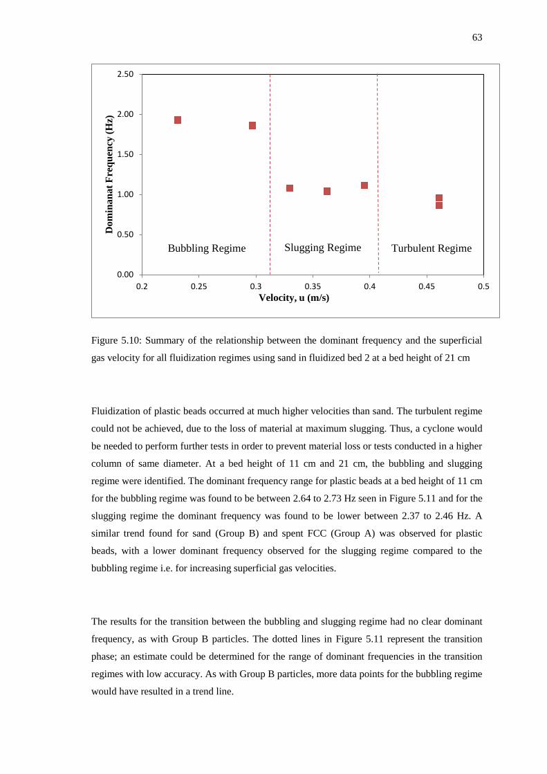
63


gas velocity for all fluidization regimes using sand in fluidized bed 2 at a bed height of 21 cm

Fluidization of plastic beads occurred at much higher velocities than sand. The turbulent regime

could not be achieved, due to the loss of material at maximum slugging. Thus, a cyclone would

be needed to perform further tests in order to prevent material loss or tests conducted in a higher

column of same diameter. At a bed height of 11 cm and 21 cm, the bubbling and slugging

regime were identified. The dominant frequency range for plastic beads at a bed height of 11 cm

for the bubbling regime was found to be between 2.64 to 2.73 Hz seen in Figure 5.11 and for the

slugging regime the dominant frequency was found to be lower between 2.37 to 2.46 Hz. A

similar trend found for sand (Group B) and spent FCC (Group A) was observed for plastic

beads, with a lower dominant frequency observed for the slugging regime compared to the

bubbling regime i.e. for increasing superficial gas velocities.

The results for the transition between the bubbling and slugging regime had no clear dominant

frequency, as with Group B particles. The dotted lines in Figure 5.11 represent the transition

phase; an estimate could be determined for the range of dominant frequencies in the transition

regimes with low accuracy. As with Group B particles, more data points for the bubbling regime

would have resulted in a trend line.

0.00

0.50

1.00

1.50

2.00

2.50

0.2 0.25 0.3 0.35 0.4 0.45 0.5

Do

min

an

at

Fre

qu

ency

(H

z)

Velocity, u (m/s)

Bubbling Regime Turbulent Regime Slugging Regime

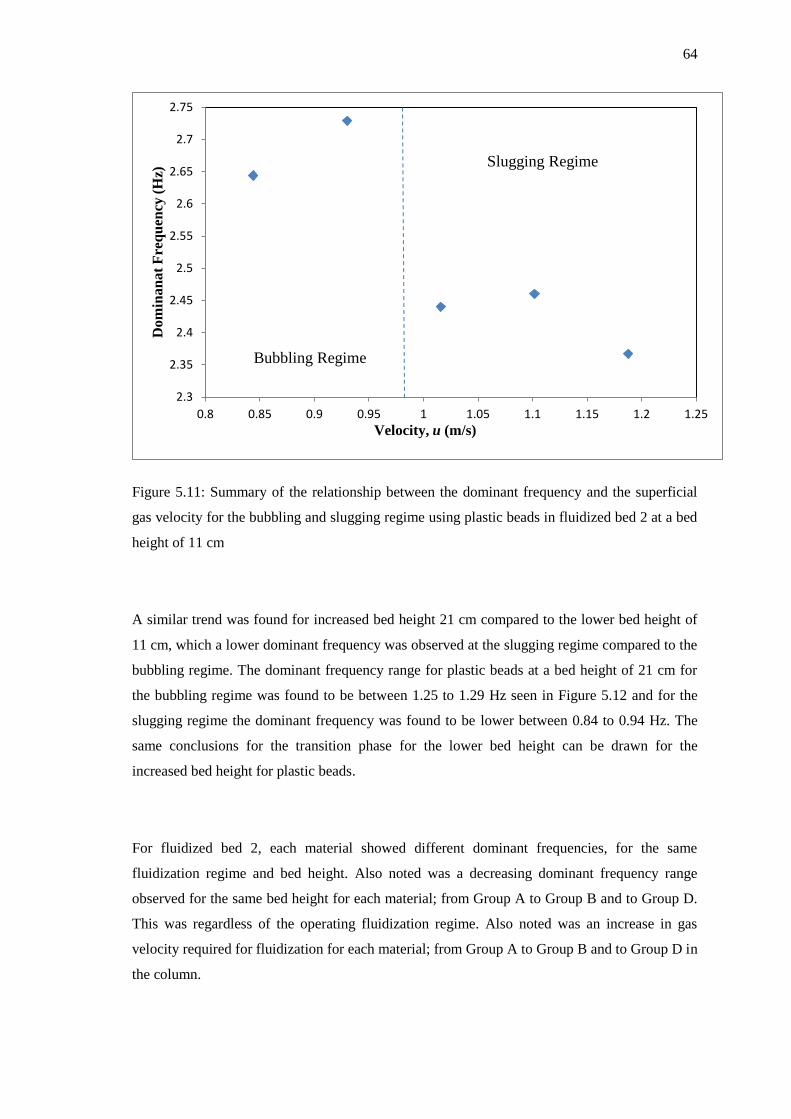
64



height of 11 cm

A similar trend was found for increased bed height 21 cm compared to the lower bed height of

11 cm, which a lower dominant frequency was observed at the slugging regime compared to the

bubbling regime. The dominant frequency range for plastic beads at a bed height of 21 cm for

the bubbling regime was found to be between 1.25 to 1.29 Hz seen in Figure 5.12 and for the

slugging regime the dominant frequency was found to be lower between 0.84 to 0.94 Hz. The

same conclusions for the transition phase for the lower bed height can be drawn for the

increased bed height for plastic beads.

For fluidized bed 2, each material showed different dominant frequencies, for the same

fluidization regime and bed height. Also noted was a decreasing dominant frequency range

observed for the same bed height for each material; from Group A to Group B and to Group D.

This was regardless of the operating fluidization regime. Also noted was an increase in gas

velocity required for fluidization for each material; from Group A to Group B and to Group D in

the column.

2.3

2.35

2.4

2.45

2.5

2.55

2.6

2.65

2.7

2.75

0.8 0.85 0.9 0.95 1 1.05 1.1 1.15 1.2 1.25

Do

min

an

at

Fre

qu

ency

(H

z)

Velocity, u (m/s)

Bubbling Regime

Slugging Regime

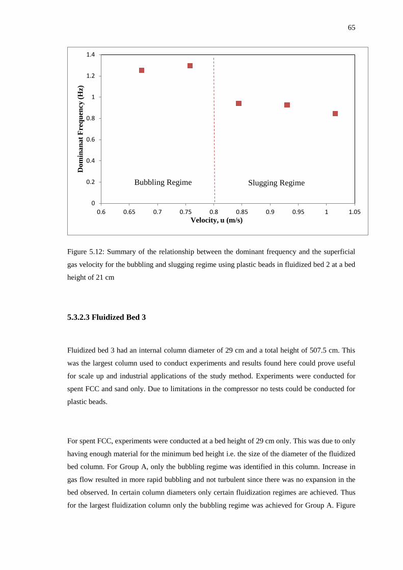
65



height of 21 cm


Fluidized bed 3 had an internal column diameter of 29 cm and a total height of 507.5 cm. This

was the largest column used to conduct experiments and results found here could prove useful

for scale up and industrial applications of the study method. Experiments were conducted for

spent FCC and sand only. Due to limitations in the compressor no tests could be conducted for

plastic beads.

For spent FCC, experiments were conducted at a bed height of 29 cm only. This was due to only

having enough material for the minimum bed height i.e. the size of the diameter of the fluidized

bed column. For Group A, only the bubbling regime was identified in this column. Increase in

gas flow resulted in more rapid bubbling and not turbulent since there was no expansion in the

bed observed. In certain column diameters only certain fluidization regimes are achieved. Thus

for the largest fluidization column only the bubbling regime was achieved for Group A. Figure

0

0.2

0.4

0.6

0.8

1

1.2

1.4

0.6 0.65 0.7 0.75 0.8 0.85 0.9 0.95 1 1.05

Do

min

an

at

Fre

qu

ency

(H

z)

Velocity, u (m/s)

Bubbling Regime Slugging Regime

66

5.13 shows the change in dominant frequency between 1.30 to 2.40 Hz within the bubbling

regime.


gas velocity for the bubbling regime using spent FCC in fluidized bed 3 at a bed height of 29 cm

For sand experiments were conducted at a bed height of 32 cm. This was due to the purposes of

comparing the results to literature found at this height. Only the bubbling regime was identified

in this column. Further identification of other regimes as in the previous fluidized bed columns

could not be identified. An increase in gas flow resulted in more rapid bubbling and not

slugging since there were no huge bubbles close to the size of the column or turbulent since

there was no expansion in the bed observed. This could have resulted due to the poor distributor

alignment which prevented the uneven gas distribution into the fluidized bed. This was evident

from the bubbles only appearing at certain sections of the column. Figure 5.14 shows the change

in dominant frequency between 0.13 to 0.22 Hz within the bubbling regime.

0

0.5

1

1.5

2

2.5

3

0.028 0.029 0.03 0.031 0.032 0.033 0.034

Dom

inan

at

Fre

qu

ency

(H

z)

Velocity, u (m/s)

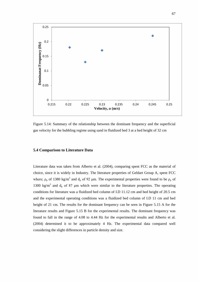
67


gas velocity for the bubbling regime using sand in fluidized bed 3 at a bed height of 32 cm

5.4 Comparison to Literature Data

Literature data was taken from Alberto et al. (2004), comparing spent FCC as the material of

choice, since it is widely in Industry. The literature properties of Geldart Group A, spent FCC

where; ρp of 1380 kg/m3 and dp of 92 μm. The experimental properties were found to be ρp of

1300 kg/m3 and dp of 87 μm which were similar to the literature properties. The operating

conditions for literature was a fluidized bed column of I.D 11.12 cm and bed height of 20.5 cm

and the experimental operating conditions was a fluidized bed column of I.D 11 cm and bed

height of 21 cm. The results for the dominant frequency can be seen in Figure 5.15 A for the

literature results and Figure 5.15 B for the experimental results. The dominant frequency was

found to fall in the range of 4.08 to 4.44 Hz for the experimental results and Alberto et al.

(2004) determined it to be approximately 4 Hz. The experimental data compared well

considering the slight differences in particle density and size.

0

0.05

0.1

0.15

0.2

0.25

0.215 0.22 0.225 0.23 0.235 0.24 0.245 0.25

Do

min

an

at

Fre

qu

ency

(H

z)

Velocity, u (m/s)

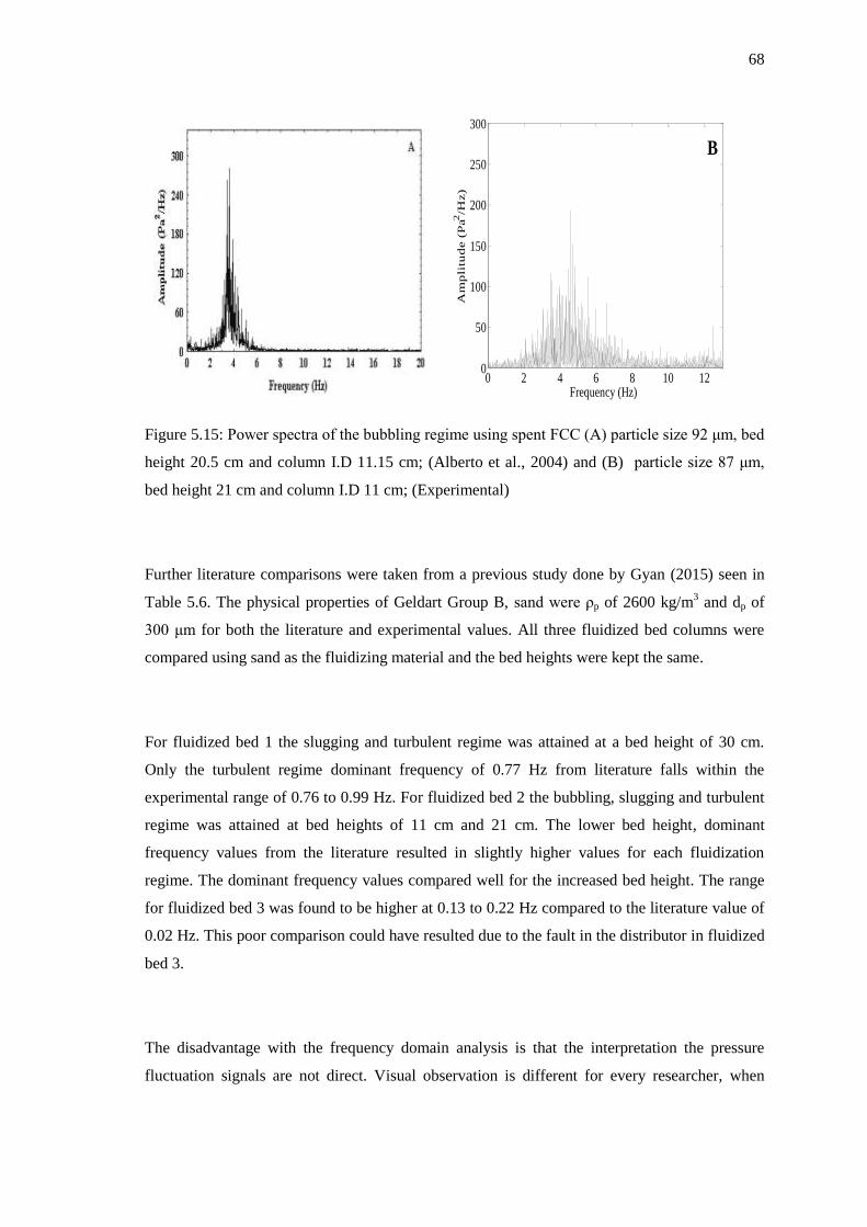
68

Figure 5.15: Power spectra of the bubbling regime using spent FCC (A) particle size 92 μm, bed

height 20.5 cm and column I.D 11.15 cm; (Alberto et al., 2004) and (B) particle size 87 μm,

bed height 21 cm and column I.D 11 cm; (Experimental)

Further literature comparisons were taken from a previous study done by Gyan (2015) seen in

Table 5.6. The physical properties of Geldart Group B, sand were ρp of 2600 kg/m3 and dp of

300 μm for both the literature and experimental values. All three fluidized bed columns were

compared using sand as the fluidizing material and the bed heights were kept the same.

For fluidized bed 1 the slugging and turbulent regime was attained at a bed height of 30 cm.

Only the turbulent regime dominant frequency of 0.77 Hz from literature falls within the

experimental range of 0.76 to 0.99 Hz. For fluidized bed 2 the bubbling, slugging and turbulent

regime was attained at bed heights of 11 cm and 21 cm. The lower bed height, dominant

frequency values from the literature resulted in slightly higher values for each fluidization

regime. The dominant frequency values compared well for the increased bed height. The range

for fluidized bed 3 was found to be higher at 0.13 to 0.22 Hz compared to the literature value of

0.02 Hz. This poor comparison could have resulted due to the fault in the distributor in fluidized

bed 3.

The disadvantage with the frequency domain analysis is that the interpretation the pressure

fluctuation signals are not direct. Visual observation is different for every researcher, when

0 2 4 6 8 10 120

50

100

150

200

250

300

Frequency (Hz)

Am

pli

tud

e (

Pa2/H

z)

B

69

accounting for each fluidization regime. Also the different operating conditions of the gas-solid

fluidized bed system are a result of the irregularities found in the comparison.

Table 5.6: Summary of the comparison of the dominant frequency for material sand in all

fluidized bed columns

Fluidized Bed

Column

Fluidization

Regime

Bed Height

(cm)

Dominant Frequency (Hz)

Experimental Range Gyan (2015)

Bed 1

I.D 5 cm

Slugging 30

1.47 - 1.51 1.34

Turbulent 0.76 - 0.99 0.77

Bed 2

I.D 11 cm

Bubbling

11

2.90 - 3.12 4.07

Slugging 2.30 - 2.57 2.63

Turbulent 2.14 - 2.15 2.44

Bubbling

21

1.86 - 1.93 1.74

Slugging 1.04 -1.17 1.13

Turbulent 0.86 - 0.95 0.98

Bed 3

I.D 29 cm Bubbling 32 0.13 - 0.22 0.02

5.5 Applicability for Scale Up

The majority of literature on scale up for fluidized beds, as discussed in Section 2.3, is focused

on equations relating to non-dimensional parameters. For successful scale-up of a fluidized bed,

the hydrodynamic scaling law delivers an effective solution. However, new developments have

shown that spectral analysis can be used to confirm scale up approaches of fluidized beds. This

method is accomplished by comparing spectra from a model prototype to a full size unit

(Nicastro & Glicksman, 1984). Fluidized bed 3 was the largest fluidized bed in the study with a

column diameter of 29 cm; therefore it was used to provide insights into this method.

For Group A material (spent FCC), the bubbling regime was the only fluidization regime

identified for fluidized beds 2 and 3. In fluidized bed 3 the dominant frequency was found

between 1.30 to 2.40 Hz for a bed height of 29 cm. The dominant frequency range for fluidized

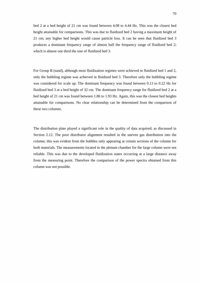
70

bed 2 at a bed height of 21 cm was found between 4.08 to 4.44 Hz. This was the closest bed

height attainable for comparisons. This was due to fluidized bed 2 having a maximum height of

21 cm; any higher bed height would cause particle loss. It can be seen that fluidized bed 3

produces a dominant frequency range of almost half the frequency range of fluidized bed 2;

which is almost one third the size of fluidized bed 3.

For Group B (sand), although most fluidization regimes were achieved in fluidized bed 1 and 2,

only the bubbling regime was achieved in fluidized bed 3. Therefore only the bubbling regime

was considered for scale up. The dominant frequency was found between 0.13 to 0.22 Hz for

fluidized bed 3 at a bed height of 32 cm. The dominant frequency range for fluidized bed 2 at a

bed height of 21 cm was found between 1.86 to 1.93 Hz. Again, this was the closest bed heights

attainable for comparisons. No clear relationship can be determined from the comparison of

these two columns.

The distribution plate played a significant role in the quality of data acquired; as discussed in

Section 2.12. The poor distributor alignment resulted in the uneven gas distribution into the

column; this was evident from the bubbles only appearing at certain sections of the column for

both materials. The measurements located in the plenum chamber for the large column were not

reliable. This was due to the developed fluidization states occurring at a large distance away

from the measuring point. Therefore the comparison of the power spectra obtained from this

column was not possible.

71

6

CHAPTER SIX

6. CONCLUSIONS

The time-series analysis of pressure fluctuation signals can be separated into three methods; the

time domain, frequency domain and state-space domain (van Ommen et al., 2011). Only the

time and frequency domain methods were investigated during this study. Firstly, the time

domain method was evaluated for the classification of each fluidization regime. The pressure

fluctuation signals obtained against time were analysed for consistent and periodic oscillations

for each specific fluidization regime. From these graphs, no irregularities in bed behaviour were

noted (van Ommen et al., 2011), thus confirming the credibility of the data received from the

data acquisition system. This also supported precise spectral analysis, as the pressure fluctuation

signal was converted into the frequency domain by use of the Fast Fourier Transform (FFT).

The time domain standard deviation technique was used to determine the transition velocity (uc)

and was found to be within the bubbling and turbulent regime velocity range.

The frequency domain technique depicts the amplitude of pressure fluctuation signals against

the dominant frequency for a particular fluidization regime. A dominant frequency is defined as

the frequency with the highest peak. In fluidized bed 1 (I.D 5 cm), no dominant frequency could

be identified for Geldart Group A and D particles, irrespective of bed height. This was due to

Group A exhibiting particulate fluidization, and Group D having a small column diameter to

large particle size ratio. Geldart Group B particles exhibited both slugging and turbulent

regimes, each being distinguished by a dominant frequency.

In fluidized bed 2 (I.D 11 cm) Geldart Group A only exhibited the bubbling regime, typical of

this material categorization, and this was effectively identified at different bed heights with a

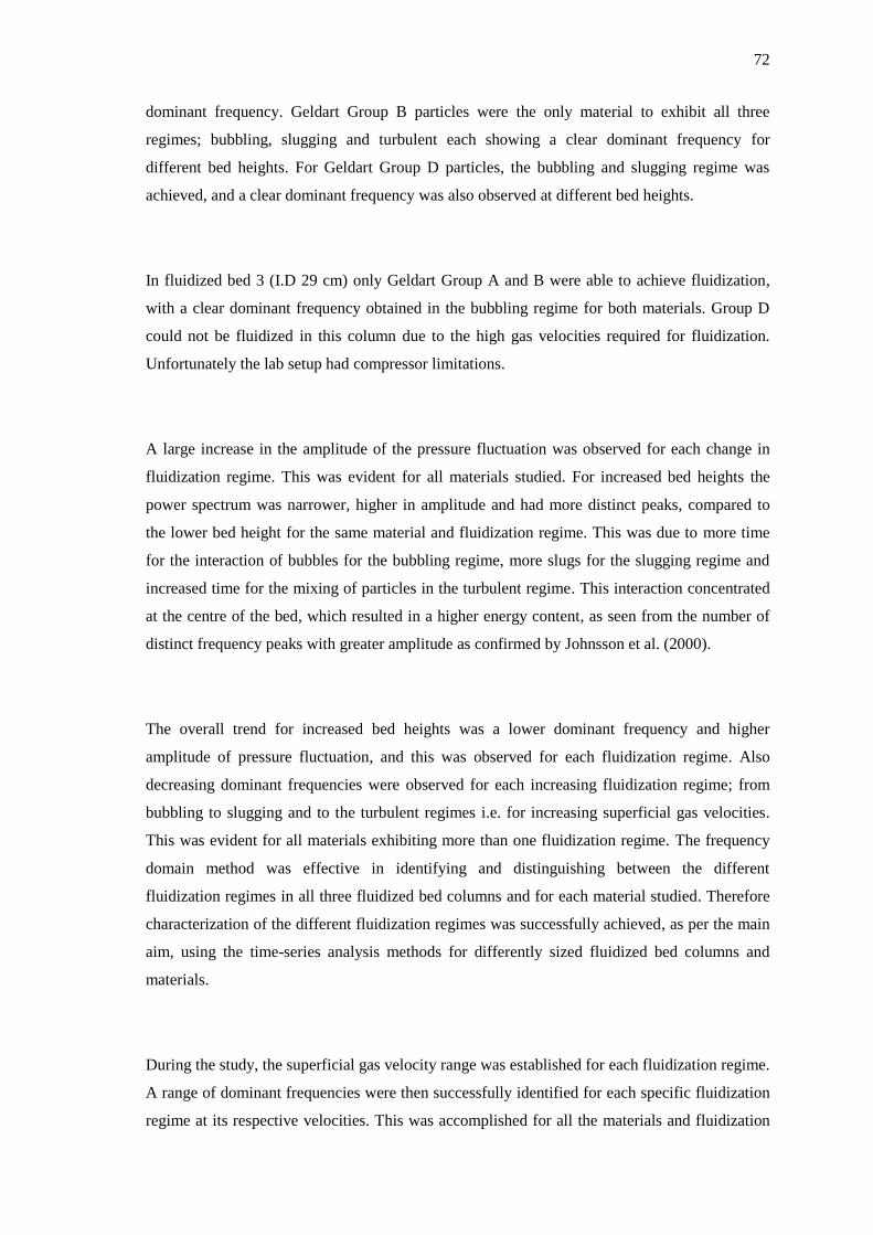
72

dominant frequency. Geldart Group B particles were the only material to exhibit all three

regimes; bubbling, slugging and turbulent each showing a clear dominant frequency for

different bed heights. For Geldart Group D particles, the bubbling and slugging regime was

achieved, and a clear dominant frequency was also observed at different bed heights.

In fluidized bed 3 (I.D 29 cm) only Geldart Group A and B were able to achieve fluidization,

with a clear dominant frequency obtained in the bubbling regime for both materials. Group D

could not be fluidized in this column due to the high gas velocities required for fluidization.

Unfortunately the lab setup had compressor limitations.

A large increase in the amplitude of the pressure fluctuation was observed for each change in

fluidization regime. This was evident for all materials studied. For increased bed heights the

power spectrum was narrower, higher in amplitude and had more distinct peaks, compared to

the lower bed height for the same material and fluidization regime. This was due to more time

for the interaction of bubbles for the bubbling regime, more slugs for the slugging regime and

increased time for the mixing of particles in the turbulent regime. This interaction concentrated

at the centre of the bed, which resulted in a higher energy content, as seen from the number of

distinct frequency peaks with greater amplitude as confirmed by Johnsson et al. (2000).

The overall trend for increased bed heights was a lower dominant frequency and higher

amplitude of pressure fluctuation, and this was observed for each fluidization regime. Also

decreasing dominant frequencies were observed for each increasing fluidization regime; from

bubbling to slugging and to the turbulent regimes i.e. for increasing superficial gas velocities.

This was evident for all materials exhibiting more than one fluidization regime. The frequency

domain method was effective in identifying and distinguishing between the different

fluidization regimes in all three fluidized bed columns and for each material studied. Therefore

characterization of the different fluidization regimes was successfully achieved, as per the main

aim, using the time-series analysis methods for differently sized fluidized bed columns and

materials.

During the study, the superficial gas velocity range was established for each fluidization regime.

A range of dominant frequencies were then successfully identified for each specific fluidization

regime at its respective velocities. This was accomplished for all the materials and fluidization

73

columns studied. Therefore the research contribution was realized for the different fluidization

regimes. In addition, these results for the dominant frequencies were plotted against the

superficial gas velocity and the transition phase for each fluidization was identified. However

the accuracy of the predicted transition phases, were constrained by the limited number of data

points, since no trend line could be established. A clear dominant frequency could not be

identified in the transition phase between the fluidization regimes using the frequency domain

method. Nevertheless the second aim, to identify the transition phase regime could be realized

with low accuracy from the research contribution.

Correlations used to predict the minimum fluidization velocity (umf) and the minimum slugging

velocity (ums) were overestimated. Operating conditions such as column diameter, type of

material and bed height had a significant influence on the hydrodynamics of the bed. This was

evident from the change in amplitude of the pressure fluctuation and shift in dominant

frequency seen for each parameter studied. The dominant frequency component was different

for each fluidization regimes achieved in the three fluidized bed columns and specific materials

studied. For fluidized bed 2, a decreasing dominant frequency range was observed for the same

bed height for each material; from Group A to Group B and to Group D. This was regardless of

the operating fluidization regime. Also noted was an increase in gas velocity required for

fluidization for each material; from Group A to Group B and to Group D in the same fluidized

bed column. The analysis showed that the change in dominant frequency was greater between

the bubbling and slugging regime, compared to the turbulent and slugging regime. The third

aim, to assess system variables impact on fluidization, was achieved as the dominant frequency

was significantly impacted by the choice of material and the bed height. This was evident as

each material showed different dominant frequencies, for the same fluidization regime and bed

height.

The forth aim was attained, as the optimum pressure probe measuring location was confirmed at

the plenum chamber. Only this location allowed for accurate data, as the other locations along

the column resulted in unusable data, due to the obstruction of the measurement point by solid

particles.

The largest column (fluidized bed 3, I.D 29 cm) was used to determine the possibility of scale

up. The poor alignment of the distribution plate on this column played a significant role in the

quality of data acquired. In addition, measurements located in the plenum chamber for the large

74

column were not reliable. This was due to the developed fluidization states occurring at a large

distance away from the measuring point. Therefore the comparison of the power spectra

obtained from this column was not possible. No conclusive results could be drawn, hence the

final aim for scale up was not realized.

In conclusion, four out of five aims were successful and the advantageous research contribution

proved to be fruitful. The learning‟s were noted and recommendations were proposed for the

unsuccessful aims for future improved studies.

75

7

CHAPTER SEVEN

7. RECOMMENDATIONS

Areas of improvement were uncovered during this study. The following recommendations are

therefore proposed to enhance further studies in gas-solid fluidized beds:

With the current experimental setup, significant fluctuations in flow readings were

displayed at higher gas velocities. Investigate another method of controlling higher gas

velocities into the fluidized bed, in order to facilitate the acquisition of more data points

for the dominant frequencies experienced at each fluidization regime. This will enable

the identification of predicted dominant frequencies at specific gas velocities.

Higher experimental gas velocities were hindered by the laboratory compressor which

was rated at 6 bar. Coupled with a standard and fixed distributor design, the largest

studied fluidized bed was negatively impacted by these constraints. It is recommended

to use a larger capacity compressor to obtain more data for larger columns. The use of

different distributor designs can be investigated to determine the effect on the

fluidization regimes.

Only one material from each of three Geldart classifications was investigated. Therefore

no intra-dependent relationships within a specific Geldart classification could be

identified. More materials from the same Geldart classification should be studied, to

compare the range of dominant frequencies obtained, for the each specific fluidization

regimes.

76

Absolute pressure measurements were employed in this study; however data accuracy

was limited in large column applications. Differential pressure measurements should be

used along larger columns to increase the accuracy of data achieved; thereby permitting

the comparison of useable power spectra results for scale-up.

77

REFERENCES

Alberto, C., Felipe, S., & Rocha, S. (2004). Time series analysis of pressure fluctuation in gas-

solid fluidized beds. Brazilian Journal of Chemical Engineering, 21(03), 497-507.

Andreux, R., Gauthier, T., Chaouki, J., & Simonin, O. (2005). New description of fluidization

regimes. AlChE Journal, 51, 1125-1130.

Baeyens, J., & Geldart, D. (1974). An investigation into slugging fluidized beds. Chemical

Engineering Science, 29, 255.

Basu, P. (2006). Combustion and Gasification in Fluidized Beds. Taylor & Francis Group.

Bi, H. T., Grace, J. R., & Lim, K. S. (1995). Transition from bubbling to turbulent fluidization.

Industrial and Engineering Chemistry Research, 34, 4003-4008.

Bi, H., Ellis, N., Abba, I., & Grace, J. (2000). A state of the art review of gas-solid turbulent

fluidization. Chemical Engineering Science, 55, 4789-4825.

Bourgeois, P., & Grenier, P. (1968). The ratio of terminal velocity to minimum fluidizing

velocity for spherical particles. Canadian Journal of Chemical Engineering, 46, 325-

328.

Cai, P., Chen, S. P., Jin, Z. Q., & Wang, Z. W. (1989). Effect of operating temperature and

pressure on the transition from bubbling to turbulent fluidization. American Institute of

Chemical Engineers, 85(270), 37-43.

Chitester, D., Kornosky, R., Fan, L., & Danko, J. (1984). Characteristics of fluidization at high

pressure. Chemical Engineering Science, 39, 253-261.

Darby, R. (2001). Chemical Engineering Fluid Mechanics (2nd ed.). New York: Marcel

Dekker.

Davidson, J. F., Clift, R., & Harrison, D. (1985). Fluidization (2nd ed.). London: Academic

Press.

Davies, C., Carroll, A., & Flemmer, R. (2008). Particle size monitoring in a fluidized bed using

pressure fluctuations. Powder Technology, 180, 307-311.

Fan, L., Ho, T., & Hiraoka, S. (1981). Pressure fluctuations in a fluidized bed. AIChE Journal,

27, 388.

78

Geankoplis, C. (2003). Transport Processes and Separation Processes Principles (Includes Unit

Operations) (Vol. IV).

Geldart, D. (1973). Types of gas fluidization. Powder Technology, 7, 285-292.

Geldart, D. (1986). Gas Fluidization Technology. New York: John Wiley & Sons.

Geldart, D., & Abrahamsen, A. (1978). Powder Technology, 19, 133.

Geldart, D., & Abrahamsen, A. (1980). Powder Technology, 26(35).

Geldart, D., & Baeyens, J. (1985). The design of distributors for gas-fluidized beds. Powder

Technology, 42, 67.

Glicksman, L., Hyre, M., & Woloshun, K. (1993). Simplified scaling relationships for fluidized

beds. Powder Technology, 77, 177-199.

Grace, J. (1982). Fluidized bed hydrodynamics. In G. Hestroni, Handbook of Multiphase

Systems (pp. 25-30). Washington D.C: Hemisphere.

Gyan, R. (2015). Time-series analysis of pressure fluctuation in gas-solid fluidized beds.

Durban: University of KwaZulu Natal.

Hilal, N., Ghannam, M., & Anabtawi, M. (2001). Effect of bed diameter, distributor and inserts

on minimum fluidization velocity. Chemical Engineering Technology, 24(2), 161-165.

Horio, M., Notaka, A., Sawa, Y., & Muchi, I. (1986). A similarity rule of fluidized bed for scale

up. AICE, 32.

Jin, Y., Yu, Z. Q., Wang, Z. W., & Cai, P. (1986). A criterion for transition from bubbling to

turbulent fluidization. Engineering Foundation.

Johnsson, F., Zijerveld, R., Schouten, J., van den Bleek, C., & Leckner, B. (2000).

Characterization of fluidization regimes by time-series analysis of pressure fluctuations.

International Journal of Multiphase Flow, 26, 663-715.

Kage, H., Agari, M., Ogura, H., & Matsuno, Y. (2000). Frequency analysis of pressure

fluctuations in fluidized bed plenum. Advanced Powder Technology, 11, 459.

Kunii, D., & Levenspiel, O. (1991). Fluidization Engineering (2nd ed.). Butterworth-

Heinemann.

Lee, G. S., & Kim, S. D. (1990). Bed expansion characteristics and transition velocity in

turbulent fluidized beds. Powder Technology, 62, 207-215.

79

Leva, M., Weintraub, M., Grummer, M., Pollchik, M., & Storch, H. H. (1951). Fluid flow

through packed and fluidized systems. U.S. Bureau of Mines Bull.

McCabe, W., Smith, J., & Harriot, P. (1985). Unit Operations of Chemical Engineering. New

York: McGraw Hill.

Nakajima, M. e. (1991). Bubble fraction and voidage in an emulsion phase in the transition to a

turbulent fluidized bed. In P. Basu, H. M., & M. Horio, Circulating Fluidized Bed (pp.

79-84). Pergamon Press.

Nicastro, M., & Glicksman, L. (1984). Experimental verification of scaling relationships for

fluidized bed. Chemical Engineering Science, 39, 1381-1391.

Pell, M. (1990). Gas Fluidization (7th ed.). New York: Elsevier Science.

Perry, R., & Green, D. (1997). Perry's Chemical Engineers' Handbook (7th ed.). New York:

McGraw Hill.

Reina, J., Velo, E., & Puigjaner, L. (2000). Predicting the minimum fluidzation velocity of

polydisperse mixtures of scrap-wood particles. Powder Technology, 111, 245-251.

Singh, R., & Roy, G. (2008). Prediction of minimum slugging velocity, bubbling index and

range of bubbling fluidization in cylindrical and non-cylindrical gas-solid fluidized

beds. Indian Journal of Chemical Engineering, 15, 85-89.

Stewart, P. S., & Davidson, J. F. (1967). Slug flow in fluidized beds. Powder Technology, 61,

61-80.

van Ommen, J. R., & Mudde, R. F. (2007). Measuring the gas-solids distribution in fluidized

beds - a review. Engineering Conferences International.

van Ommen, J., Sasic, S., Van der Schaaf, J., Gheorghiu, S., & Johnsson, F. (2011). Time-series

analysis of pressure fluctuations in gas-solid fluidized beds - A review. International

Journal of Multiphase Flow, 37, 403-428.

Wen, C., & Yu, Y. (1966). A generalized method for predicting the minimum fluidization

velocity. American Institute of Chemical Engineeers, 12, 610-612.

Yang, W. (2003). Bubbling Fluidized Beds. In W. Yang, Handbook of Fluidization and Fluid-

Particle Systems (pp. 53-112). New York: Marcel Dekker.

Yang, W. C. (1976). BHRA Fluid Engineering. In Proceedings of the pneumotransport 3 (pp. 5-

49). Bedford.

80

A

APPENDIX A

ADDITIONAL TIME DOMAIN RESULTS

The results presented in this appendix are an extension of chapter 5.2.1 for fluidized bed 2 since

all materials and their respective regimes and transition regimes were able to be established in

this column. The results illustrate the time-series of the pressure fluctuations measured in each

of the different regimes; bubbling, slugging and turbulent as well as the transition regimes using

the three fluidizing materials; spent FCC, sand and plastic beads in fluidized bed 2 at a bed

height of 11 cm and 21 cm. These results indicate the influence of bed height, which in all cases

show that a higher amplitude is achieved at increased bed heights.


spent FCC in fluidized bed 2 at the indicated bed heights

101000

101500

102000

102500

103000

0 2 4 6 8 10

Pre

ssu

re (

Pa)

Time (s)

Bubbling Height 11 cm


81

Figure A.2: Time-series of the pressure fluctuations measured in the bubbling regime using sand

in fluidized bed 2 at the indicated bed heights

Figure A.3: Time-series of the pressure fluctuations measured in the slugging regime using sand

in fluidized bed 2 at the indicated bed heights

102000

103000

104000

105000

106000

107000

108000

0 2 4 6 8 10

Pre

ssu

re (

Pa

)

Time (s)



102000

104000

106000

108000

110000

112000

0 2 4 6 8 10

Pre

ssu

re (

Pa)

Time (s)

Slugging Height 11 cm

Slugging Height 21 cm

82

Figure A.4: Time-series of the pressure fluctuations measured in the turbulent regime using

sand in fluidized bed 2 at the indicated bed heights


slugging regime using sand in fluidized bed 2 at the indicated bed heights

104000

108000

112000

116000

0 2 4 6 8 10

Pre

ssu

re (

Pa

)

Time (s)

Turbulent Height 11 cm

Turbulent Height 21 cm

103000

104000

105000

106000

107000

108000

109000

0 2 4 6 8 10

Pre

ssu

re (

Pa)

Time (s)

Bubbling to Slugging Height 11cm

Bubbling to Slugging Height 21cm

83

Figure A.6: Time-series of the pressure fluctuations measured in the transition from slugging to

turbulent regime using sand in fluidized bed 2 at the indicated bed heights


plastic beads in fluidized bed 2 at the indicated bed heights

104000

105000

106000

107000

108000

109000

110000

111000

112000

0 2 4 6 8 10

Pre

ssu

re (

Pa

)

Time (s)

Slugging to Turbulent Height 11cm

Slugging to Turbulent Height 21cm

112000

114000

116000

0 2 4 6 8 10

Pre

ssu

re (

Pa)

Time (s)



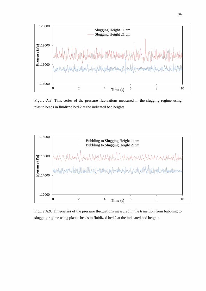
84

Figure A.8: Time-series of the pressure fluctuations measured in the slugging regime using

plastic beads in fluidized bed 2 at the indicated bed heights


slugging regime using plastic beads in fluidized bed 2 at the indicated bed heights

114000

116000

118000

120000

0 2 4 6 8 10

Pre

ssu

re (

Pa

)

Time (s)

Slugging Height 11 cmSlugging Height 21 cm

112000

114000

116000

118000

0 2 4 6 8 10

Pre

ssu

re (

Pa)

Time (s)

Bubbling to Slugging Height 11cmBubbling to Slugging Height 21cm

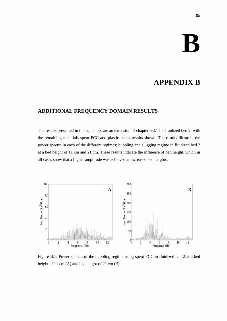
85

B

APPENDIX B

ADDITIONAL FREQUENCY DOMAIN RESULTS

The results presented in this appendix are an extension of chapter 5.3.1 for fluidized bed 2, with

the remaining materials spent FCC and plastic beads results shown. The results illustrate the

power spectra in each of the different regimes; bubbling and slugging regime in fluidized bed 2

at a bed height of 11 cm and 21 cm. These results indicate the influence of bed height, which in

all cases show that a higher amplitude was achieved at increased bed heights.

Figure B.1: Power spectra of the bubbling regime using spent FCC in fluidized bed 2 at a bed

height of 11 cm (A) and bed height of 21 cm (B)

0 2 4 6 8 10 120

20

40

60

80

100

Frequency (Hz)

Am

pli

tud

e (

Pa2

/Hz)

A

0 2 4 6 8 10 120

50

100

150

200

250

300

Frequency (Hz)

Am

pli

tud

e (

Pa2

/Hz)

B

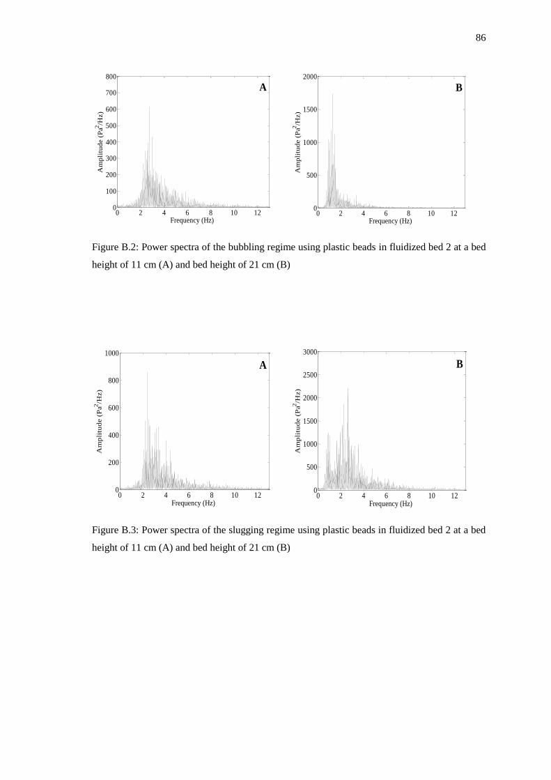
86

Figure B.2: Power spectra of the bubbling regime using plastic beads in fluidized bed 2 at a bed


Figure B.3: Power spectra of the slugging regime using plastic beads in fluidized bed 2 at a bed


0 2 4 6 8 10 120

100

200

300

400

500

600

700

800

Frequency (Hz)

Am

pli

tud

e (

Pa2

/Hz)

A

0 2 4 6 8 10 120

500

1000

1500

2000

Frequency (Hz)

Am

pli

tud

e (

Pa2

/Hz)

B

0 2 4 6 8 10 120

200

400

600

800

1000

Frequency (Hz)

Am

pli

tud

e (

Pa2

/Hz)

A

0 2 4 6 8 10 120

500

1000

1500

2000

2500

3000

Frequency (Hz)

Am

pli

tud

e (

Pa2

/Hz)

B

87

C

APPENDIX C

MATLAB CODE FOR IMPLEMENTATION OF THE FAST

FOURIER TRANSFORM

The Fast Fourier Transform (FFT) is a mathematical tool that is used to transform a signal from

a function of time to a signal of a function of frequency thus enabling the analysis in the

frequency domain. MATLAB has a built in function that is capable of computing large amounts

of data to calculate the FFT. A simulation code for a single run broken up into eight segments is

given below. The same code is implemented for additional runs and different operating

conditions; with the Microsoft Excel data file changed each time.

clc

% Specify experimental data file and sheet from Microsoft Excel

File = 'C:\MATLAB7\work\Sand ID2 H1.xls';

Sheet = 'B Run1';

% Specify number of data points and interval time per segment

N = 6000;

T = 225;

% Calculate the FFT for each segment

Data1='A3:A6003';

Press1 = xlsread(File,Sheet,Data1);

Pressure1 = Press1;

88

P1 = abs(fft(Pressure1))/(N/2);

P1 = P1(2:N/2).^2;

Data2='A6004:A12004';


Pressure2 = Press2;


P2 = P2(2:N/2).^2;

Data3='A12005:A18005';


Pressure3 = Press3;


P3 = P3(2:N/2).^2;

Data4='A18006:A24006';


Pressure4 = Press4;


P4 = P4(2:N/2).^2;

Data5='A24007:A30007';


Pressure5 = Press5;


P5 = P5(2:N/2).^2;

Data6='A30008:A36008';


Pressure6 = Press6;


P6 = P6(2:N/2).^2;

Data7='A36009:A42009';


Pressure7 = Press7;


P7 = P7(2:N/2).^2;

Data8='A42010:A48010';


Pressure8 = Press8;


P8 = P8(2:N/2).^2;

% Calculate the frequency

freq = [1:N/2-1]/T;

% Plot the power spectrum for each segment

figure

subplot(2,4,1)

plot(freq,P1,'k')

axis([0 13 0 500])

set(get(gcf,'CurrentAxes'),'FontName','Times New Roman','FontSize',20)

xlabel('Frequency (Hz) ')

89


ylabel('Amplitude (Pa^2/Hz)')

subplot(2,4,2)

plot(freq,P2,'k')

axis([0 13 0 500])

set(get(gcf,'CurrentAxes'),'FontName''Times New Roman','FontSize',20)




subplot(2,4,3)

plot(freq,P3,'k')

axis([0 13 0 500])





subplot(2,4,4)

plot(freq,P4,'k')

axis([0 13 0 500])





subplot(2,4,5)

plot(freq,P5,'k')

axis([0 13 0 500])





subplot(2,4,6)

plot(freq,P6,'k')

axis([0 13 0 500])





subplot(2,4,7)

plot(freq,P7,'k')

axis([0 13 0 500])





subplot(2,4,8)

plot(freq,P8,'k')

axis([0 13 0 500])





90

D

APPENDIX D

PARTICLE SIZE RESULTS

The results presented in this appendix are an extension of chapter 4.1.2.2. The results are

illustrated for Geldart Group A particles (spent FCC), in which a Shimadzu SALD-3101 laser

diffraction particle size analyser was used to determine the particle size.

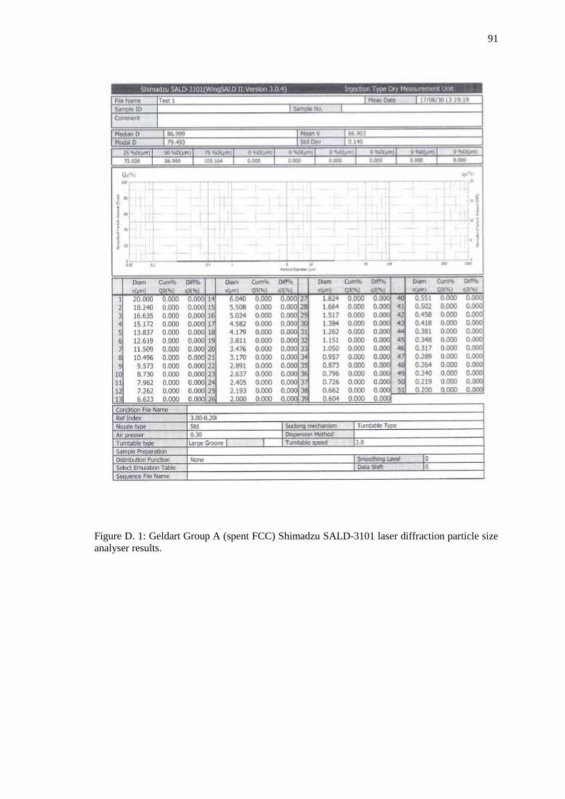
91

Figure D. 1: Geldart Group A (spent FCC) Shimadzu SALD-3101 laser diffraction particle size

analyser results.

characterization of fluidization regimes by analysis …

Documents