chapter8 learning to reason about distributionreed/instructors/math 10041... · 166 8 learning to...

Chapter 8Learning to Reason About Distribution

Statisticians look at variation through a lens which is“distribution”.

(Wild, 2006, p. 11)

Snapshot of a Research-Based Activity on Distribution

Groups of three to four students are each given an envelope containing 21 differ-ent pieces of paper, each with a different histogram printed on it. Students sort thegraphs into piles, so that the graphs in each pile have a similar shape. After sortingthem into the piles (e.g., normal/bell-shaped, left-skewed, right-skewed, bimodal,and uniform), students choose one histogram from each pile that best representsthat category, and these selections are shared and discussed as a class. Students usetheir own informal language to “name” each shape: bell-shaped, bunched to oneside, like a ski slope, camel humps, flat, etc. These informal names are matched tothe formal statistical terms such as normal, skewed, bimodal, and uniform. Finally,students consider which terms are characteristics (e.g., skewness) that can apply tographs in more than one category (e.g., a distribution that is skewed and bimodal)vs. those that can only be labeled by one name (e.g., uniform or normal distribution).

Rationale for This Activity

Although this activity may seem like a game for elementary school students, theactivity involves some important challenges and learning outcomes for high schooland college students in a first statistics course. First of all, this activity helps studentslook at histograms as an entity, rather than as a set of data values and cases, whichresearch has shown to be a key problem in reasoning about distributions. Secondly,students often fail to see the general shape of distributions, because of the effects ofrandomness (the “noise”); and expect to see perfect shapes like the models given intheir textbooks. This activity helps them see that there are many types of “normal”distributions or skewed distributions. They learn to look beyond the individual fea-tures of the graph and see the more general or global characteristics. Finally, thisactivity focuses on the language used to describe distributions, which can often beconfusing to students. The word “normal” in statistics refers to a bell-shaped curve

J.B. Garfield, D. Ben-Zvi, Developing Students’ Statistical Reasoning,C© Springer Science+Business Media B.V. 2008

165

166 8 Learning to Reason About Distribution

that has certain characteristics while in everyday life it means typical or not unusual.Students can take an informal name of a shape (e.g., ski slope for a right-skeweddistribution) and map them to the correct statistical labels, which can then be usedto help remind them of the statistical term (e.g., a teacher talking about a skewedcurve can say, “remember it is like a ski slope”).

The Importance of Understanding Distribution

We begin this section with a poignant illustration, offered by Bill Finzer to par-ticipants at the Fourth International Research Forum on Statistical Reasoning,Thinking, and Literacy, the focus of which was on “Reasoning about Distribution”(Makar, 2005)

The Little Prince, by de Saint-Exupery (2000) begins with this drawing.

To adults, the drawing looked exactly like a hat.To the child artist who drew it and to the little prince, it was a drawing of aboa that had eaten an elephant.

If the little prince showed this picture to a statistician, he would say: “Thisrepresents a distribution of data.”

We like this example because it shows how statisticians look at irregular shapes ofdata sets and look beyond the details to see a general shape and structure. This isusually a first step in any data analysis and leads to important questions about the

The Place of Distribution in the Curriculum 167

data to be analyzed, such as: What mechanism or process might have led to thisshape? Are there any values that need to be investigated (e.g., possible outliers)?

A graph of a distribution reveals variation of a quantitative variable. Accordingto Wild (2006), statisticians respond to the “omnipresence of variability” in data(Cobb & Moore, 1997) by investigating, disentangling, and modeling patterns ofvariation represented by distributions of data. He suggests that statisticians look atvariation through a lens that is “distribution.”

Students encounter two main types of “distribution” in an introductory statisticsclass. The first type is distributions of sample data that students learn to graph, de-scribe, and interpret. These are empirical distributions of some particular measuredquantity. The second type of distribution encountered is a theoretical one, e.g., nor-mal or binomial distributions, which are actually probability models (Wild, 2006).

Although the two types share many common features (e.g., they can be describedin terms of shape, center, and spread), it is important to help students distinguish be-tween them because of the way in which we use them. The distinction that underliesempirical versus theoretical distributions relates to variation. When examining anempirical distribution, the focus is on description and interpretation of the messagein the data, and thinking about what model may fit or explain the variation of thedata. Theoretical distributions are models to fit to data, to help explain, estimate,or make predictions about the variability of empirical data. Yet, a third type ofdistribution, students encounter in a statistics course is a distribution made up ofsample statistics, which again has both empirical and theoretical versions. Thesesampling distributions are discussed in detail in Chapter 12.

The Place of Distribution in the Curriculum

Empirical distributions are the foundation of students’ work in an introductorystatistics course, either beginning a course or following a unit on collecting andproducing data (experiments and surveys, Chapter 6). This chapter focuses mainlyon teaching and learning issues related to empirical distributions, while Chapters 7and 12, respectively, also discuss theoretical distributions. In addition, this chapterfocuses on understanding a single distribution, primarily in the form of dotplotsand histograms, while Chapter 11 examines these graphs along with boxplots in thecomparison of two or more distributions.

The methods of Exploratory Data Analysis introduced by Tukey (1977) have hada big impact on the way distributions are taught in today’s courses. Students usemany ideas and tools to explore data and learn to think of data analysis as detectivework. Students usually learn multiple ways to graph data sets by hand and on thecomputer. These methods include dotplots (also called line plots), stem and leafplots, histograms, and boxplots. Students learn that different graphs of a data setreveal different characteristics of the data. For example, a histogram or dotplot givesa better idea of the shape of a data set, while a boxplot is often better at revealingan outlier. A stem-and-leaf plot or dotplot may give a better idea of where there areclumps or gaps in the distribution.


Current statistical software programs (e.g., TinkerPlots, Fathom) allow studentsto easily manipulate data representations, for example, to transform one graph ofa data set to another, display several interlinked graphs of the same data set onone screen (a change in one will show in the others), and some allow students tohighlight particular data values and see where they are located in each graph. Theseexplorations are used to ask questions about the data: What causes gaps and clusters?Are outliers real data values or errors in data collection or coding? What factors mayhelp explain the features revealed in a graph of a distribution? In most introductorycourses along with learning how to graph distributions of data, students are taughtto look for specific features of distributions and begin to describe them informally(e.g., estimate center and range) and then more formally (e.g., shape, center, andspread).

Distribution is one of the most important “big ideas” in a statistics class. Ratherthan introduce this idea early in a class and then leave it behind, today’s more inno-vative curriculum and courses have students constantly revisit and discuss graphicalrepresentations of data, before any data analysis or inferential procedure. In a similarvein, the ideas of distributions having characteristics of shape, center, and spread canbe revisited when students encounter theoretical distributions and sampling distri-butions later in the statistics course.

Review of the Literature Related to ReasoningAbout Distribution

The research literature provides a strong case that understanding of distributions,even in the simplest forms, is much more complex and difficult than many statisticsteachers believe. Although little of the research includes college students, the resultsof studies on precollege level students and precollege level teachers demonstrate thedifficulty of learning this concept, some common misconceptions, and incompleteor shallow understandings that we believe also apply to college students.

Much of the research on distribution emerged because of the consensus in thestatistics education community that it is a basic building block for a web of key sta-tistical ideas, such as variability, sampling, and inference (e.g., Garfield & Ben-Zvi,2004; Pfannkuch & Reading, 2006). Other studies (e.g., Reading & Shaughnessy,2004; Watson, 2004) focused on broader questions than how students reason aboutdistribution, but yielded relevant results. For example, Chance et al. (2004) assertthat the knowledge of distribution and understanding of histograms are necessaryprerequisites to learning and understanding sampling distributions.

Developing an Aggregate View of Distribution

A major outcome of several studies on how students solve statistical problems isthat they tend not to see a data set (statistical distribution) as aggregate, but rather

Review of the Literature Related to ReasoningAbout Distribution 169

as individual values (e.g., Hancock, Kaput, & Goldsmith, 1992). Konold & Higgins(2003) claimed that, “students need to make a conceptual leap to move from seeingdata as an amalgam of individuals each with its own characteristics to seeing thedata as an aggregate, a group with emergent properties that often are not evident inany individual member” (p. 202). They explained this challenging transition in thefollowing way:

With the individuals as the foci, it is difficult to see the forest for the trees. If the data valuesstudents are considering vary, however, why should they regard or think about those valuesas a whole? Furthermore, the answers to many of the questions that interested students—for instance, Who is tallest? Who has the most? Who else is like me?—require locatingindividuals, especially themselves, within the group. We should not expect students to beginfocusing on group characteristics until they have a reason to do so, until they have a questionwhose answer requires describing features of the distribution. (Konold and Higgins, 2003,p. 203)

To explore the emergence of second graders’ informal reasoning about distribution,Ben-Zvi and Amir (2005) studied the ways in which three second grade students(age 7) started to develop informal views of distributions while investigating realdata sets. They described what it may mean to begin reasoning about distribution byyoung students, including two contrasting distributional conceptions: “flat distribu-tion” and “distributional sense”. In the “flat distribution” students focused just on thevalues of distribution and did not refer at all to their frequencies, while students whostarted acquiring a “distribution sense” showed an appreciation and understandingthat a distribution of a variable tells us what values it takes and how often it takesthese values. The gradual transfer from the incomplete perception of a distributiontowards the more formal sense of distribution presented an immense challenge tothese students.

In a teaching experiment with older students (seventh grade students in Israel),Ben-Zvi and Arcavi (2001) show how students were able to make a transition fromlocal to global reasoning, from individual-based to aggregate-based reasoning.The researchers found that carefully designed tasks (e.g., comparing distributions,handling outliers), teachers’ guidance and challenging questions, along with mo-tivating data sets and appropriate technological tools helped students to make thistransition.

Konold, Pollatsek, Well, and Gagnon (1997) interviewed two pairs of high-school students who had just completed a year-long course in probability and statis-tics. Using software and a large data set students had used as part of the course,these students were asked to explore the data and respond to different questionsabout the data and to support their answers with data summaries and graphs. Theresults suggest that students had difficulty in thinking about distributions and insteadfocused on individual cases. They did not use the methods and statistics learned inthe course when comparing two distributions, but instead relied on more intuitivemethods involving comparisons of individual cases or homogeneous groups of casesin each group. Results were re-analyzed along with results from two other studies(Konold, Higgins, Russell, & Khalil, 2003) and the following types of responseswere suggested as ways students reason about a distribution of data.


1. Seeing data as Pointers (to the larger event from which the data came).2. Seeing data as Case-values (values of an attribute for each case in the data set).3. Seeing data as Classifiers (giving frequency of cases for a particular value).4. Seeing data as an Aggregate (the distribution as an entity with characteristics

such as shape, center, and spread).

The authors note that although an important goal in statistics is to help students seea distribution as an aggregate, they feel it is important to pay attention to students’initial views of data and to carefully help them gradually develop the aggregate view(Konold et al., 2003).

Understanding the Characteristics of a Distribution

Several studies focused on how students come to conceive of shape, center, andspread as characteristics of a distribution and look at data with a notion of distribu-tion as an organizing structure or a conceptual entity. For example, based on theiranalysis of students’ responses on the National Assessment of Educational Progress(NAEP) over the past 15 years, Zawojewski and Shaughnessy (2000) suggest thatstudents have some difficulty finding the mean and the median as well as difficultyselecting appropriate statistics. They explain that one of the reasons that studentsdo not find the concepts of mean and median easy may be that they have not hadsufficient opportunities to make connections between centers and spreads; that is,they have not made the link between the measures of central tendency and thedistribution of the data set. Mokros and Russell (1995) claim that students needa notion of distribution before they can sensibly choose between measures of centerand perceive them as “representatives” of a distribution.

Reasoning About Graphical Representations of Distributions

One of the difficulties in learning about graphical representations of distributionsis confusion with bar graphs. In elementary school, students may use bars to rep-resent the value of an individual case (e.g., number of family pets), or a bar canrepresent the frequency of a value (e.g., number of families with one pet). Today,some statistics educators distinguish between these two types of representations,referring to case-value plots as the graphs where a line or bar represents the valueof an individual case, or student. In contrast, the bars of a histogram represent aset of data points in an interval of values. While case-value and bar graphs canbe arranged in any order (e.g., from smallest to largest or alphabetical by label),bars in a histogram have a fixed order, based on the numerical (horizontal) scale.Furthermore, while the vertical scale of a histogram is used to indicate frequencyor proportion of values in a bar (interval), the vertical scale for a bar graph mayrepresent either a frequency or proportion for a category of categorical data, or itmay represent magnitude (value of a case presented by that bar). These differencescan cause confusion in students, leading them to try to describe shape, center, and


spread of bar graphs or to think that bars in a histogram indicate the magnitude ofsingle values (Bright & Friel, 1998).

Establishing connections among data representations is critical for developingunderstanding of graphs; however, students cannot make these connections easilyand quickly. To find instructional strategies that help learners understand the impor-tant features of data representations and the connections among them, Bright andFriel (1998) studied ways that students in grades 6, 7, and 8 make sense of informa-tion in graphs and connections between pairs of graphs. They report that studentsbenefited from these activities by recognizing the importance of “the changing rolesof plot elements and axes across representations”, and, therefore, suggest that teach-ers need to “provide learners with opportunities to compare multiple representationsof the same data set” (p. 87). They also suggest to promote rich discourse about dis-tributions of data in the classroom to help students understand the important aspectsof each representation.

Students’ recognition of graphical aspects of a distribution as an entity wasstudied by Ainley, Nardi, and Pratt (2000). They observed young students (8–12years) who collected data during ongoing simple experiments and entered themin spreadsheets. They noted that despite limited knowledge about graphs, studentswere able to recognize abnormalities (such as measurement errors) in graphs andto take remedial action by adjusting the graphs toward some perceived norm. Theresearchers have labeled this behavior, “normalizing,” an activity in which childrenconstruct meanings for a trend in data and in graphs. Ainley and her colleagues claimthat children gained this intuitive sense of regularity from everyday experience,experience gained during the activity, their sense of pattern, or from an emergingperception of an underlying mathematical model. The researchers recommend theuse of computer-rich pedagogical settings to change the way in which knowledgeabout data graphs is constructed.

Helping Students to Reason with Graphs of Distributions

Students often see and use graphs as illustrations rather than as reasoning tools tolearn something about a data set or gain new information about a particular prob-lem or context (Wild & Pfannkuch, 1999; Konold & Pollatsek, 2002). Current re-search on students’ statistical understanding of distribution (e.g., Pfannkuch, 2005a;Watson, 2005) recommends a shift of instructional focus from drawing various kindsof graphs and learning graphing skills to making sense of the data, for detecting anddiscovering patterns, for confirming or generating hypotheses, for noticing the unex-pected, and for unlocking the stories in the data. It has been suggested that reasoningwith shapes forms the basis of reasoning about distributions (Bakker, 2004a; Bakkerand Gravemeijer, 2004).

Others refer to developing skills of visual decoding, judgment, and contextas three critical factors in helping students derive meaning from graphs (Friel,Curcio and Bright, 2001). Reasoning about distributions is more than reasoningabout shapes. It is about decoding the shapes by using deliberate strategies to


comprehend the distributions and by being cognizant of the many referents, whichare bound within the distributions. Furthermore, students have to weigh the evidenceto form an opinion on and inference from the information contained in the distribu-tions (Friel et al., 2001). Such informal decision-making under uncertainty requiresqualitative judgments, which are much harder than the quantitative judgments madeby statistical tests (Pfannkuch, 2005a).

In one of the rare studies at the college level, delMas, Garfield, and Ooms(2005) analyzed student performance on a series of multiple-choice items assess-ing students’ statistical literacy and reasoning about graphical representations ofdistribution. They found that college students, like younger peers in middle schooldescribed above, confused bar graphs and histograms, thinking that a bar graph ofindividual cases, with categories on the horizontal scale, could be used to estimateshape, center, and spread. They also thought that such a bar graph might look likethe normal distribution. They tended to view flat, rectangular-shaped histograms asa time series plot showing no variation, when these graphs typically show muchvariation in values. The researchers also identified errors students make in readingand interpreting horizontal and vertical axes. Based on the difficulties students ap-peared to have reading and interpreting histograms, the authors questioned whetherstudents should be taught to use only dotplots and boxplots to represent data sets.After questioning colleagues, they concluded that there were important reasons tokeep histograms in the curriculum as a way of representing distributions of data,because of the need for students to understand the ideas of area and density requiredfor understanding theoretical distributions, and because dotplots are not feasible forvery large data sets.

Technological Tools to Develop the Concept of Distribution

Technology can play an important role in developing distributional reasoning byproviding easy access to multiple representations and endless opportunities to in-teractively manipulate and compare representations of the same data set. However,this is not a simple task. Biehler (1997b) reports that despite using an innovativesoftware tool to generate and move between different graphs of data, interpretingand verbally describing these graphs were profoundly difficult for high school andcollege students, unless they had a conceptual understanding of the foundationalconcepts.

To study the impact of technology on distributional understanding, Cobb (1999),McClain & Cobb (2001), and Bakker & Gravemeijer (2004) examined how a hy-pothetical learning trajectory, translated into a particular instructional sequence,involving the use of Minitools (Cobb et al., 1997) supported the development ofstudents’ statistical reasoning about distribution. Minitools are simple but inno-vative Web applets that were designed and used to assist students to develop theconcept of distribution. Results of these teaching experiments suggest that students’development of relatively deep understandings of univariate distribution are feasiblegoals at the middle school level, when activities, discussion, and tools are used inparticular ways.


Fig. 8.1 Life span ofbatteries displayed by acase-value bar graph inMinitool 1 (sorted by size).Each horizontal barrepresents the life span inhours for a particular battery

For example, one aspect of distribution, shape, can be seen by looking athistograms or dotplots. To understand what dots in a dotplot represent, studentsneed to realize that a dot corresponds to a value of a particular variable, and eachdot represents one case that has that particular value. To help students develop thisinsight, a tool shows them case-value bars (Minitool 1, see Fig. 8.1). These barsseem to correspond to students’ intuitive ways of organizing and displaying a set ofdata. Students then are helped to make a transition to a second Minitool (Fig. 8.2),which takes the end points of the case-value bars and stacks them in a dotplot. Whileeach case in Minitool 1 is represented by a bar whose relative length corresponds tothe value of the case, each case in Minitool 2 is represented by a dot in a dotplot.Figures 8.1 and 8.2 display just one data set at a time; however, all given data setsin Minitools include two groups (e.g., comparing two brands of batteries), whichbetter help students develop distributional reasoning.

Minitool 2 has options to organize data in ways that can help students developtheir understanding of distributions. For example, the dotplot can be divided intoequal groups or into equal intervals, which support the development of an under-standing of the median and quartiles, boxplot, density, and histogram, respectively

Fig. 8.2 The same data set oflife span of batteriesdisplayed by a dotplot inMinitool 2


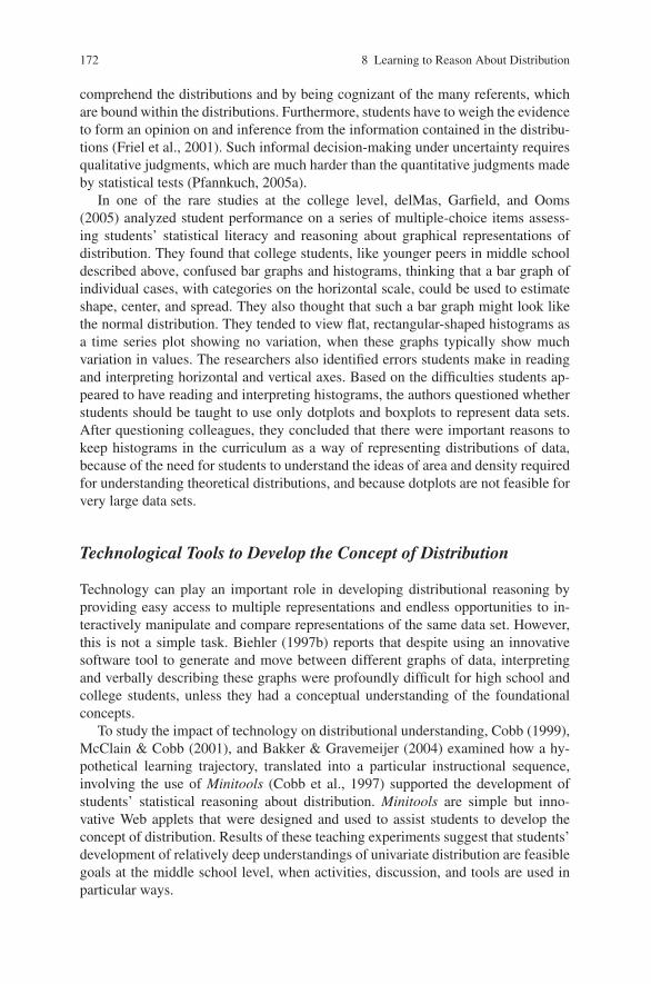
Fig. 8.3 (a) Four equal group and boxplot overlay option with and without data. (b) Fixed intervalwidth and histogram overlay options with and without data

(see Fig. 8.3). Many of the features of the Minitools have been incorporated into therecently published TinkerPlots software (Konold & Miller, 2005).

The combination of the two Minitools graphs was found to be useful in helpingstudents develop the idea of distribution. Bakker and Gravemeijer (2004) identifiedpatterns of student answers and categorized an evolving learning trajectory that hadthree stages: Working with graphs in which data were represented by horizontal bars(Minitool 1, Fig. 8.1), working with dotplots (Minitool 2, Fig. 8.2), and focusingon characteristics of the data set, such as bumps, clusters, and outliers using bothMinitools.

Based on their research, Bakker and Gravemeijer (2004) suggest several promis-ing instructional heuristics to support students’ aggregate reasoning of distributions:(1) Letting students invent their own data sets could stimulate them to think of adata set as a whole instead of individual data points. (2) Growing samples, i.e.,

Implications of the Research: Teaching Students to Reason About Distribution 175

letting students reason with stable features of variable processes, and compare theirconjectured graphs with those generated from real graphs of data. (3) Predictionsabout the shape and location of distributions in hypothetical situations. All thesemethods can help students to look at global features of distributions and foster amore global view.

Implications of the Research: Teaching Students to ReasonAbout Distribution

The results of these studies suggest in general that it takes time for students to de-velop the idea of distribution as an entity, and that they need repeated practicing inexamining, interpreting, discussing, and comparing graphs of data. It is important toprovide opportunities for students to build on their own intuitive ideas about waysto graph distributions of data. Some of the research suggests that students use theirown informal language (e.g., talking about ‘bumps’ and ‘clumps’ of data) beforelearning more formal ones (e.g., mode, skewness). The research also suggests thatteachers begin having students use graphical representations of data that show all thedata values (e.g., dotplots or stem-and-leaf plots) and carefully move from these tomore abstract and complex graphs that hide the data (e.g., histograms and boxplots),showing how different graphs represent the same data. Several studies suggest asequence of activities that leads students from individual cases (case-value bars) todotplots to groups of data points (clusters in intervals) to histograms. This sequencecan later be used to develop the idea of a boxplot (see Chapter 11). New computertools (e.g., Minitools, TinkerPlots, and Fathom) show promise for helping to guidestudents through this process and to allow them to connect different graphical rep-resentations of distributions.

Teaching Students the Concept of Distribution

The strongest message in the research on understanding graphs and distributionsis that statistics teachers need to be aware of the difficulties students have devel-oping the concept of distribution as an entity, with characteristics such as shape,center, and spread. While most textbooks begin a unit on descriptive statistics withgraphs of data, when to use them, how to construct them and how to determineshape, estimate center and spread, we believe that there are some important steps toprecede this. We think it is best to begin data explorations with case-value barsthat represent individual cases, a type of graph students are very familiar withand that is more intuitive for them to understand and interpret. Then, this type ofgraph can be transformed to a dotplot using diagrams or a tool such as Tinker-Plots. For example, a diagram of case-value bars such as the one shown below(Fig. 8.4), for a set of students test scores, can be converted by the students toa dotplot (Fig. 8.5), taking the end point of each case-value and plotting it on adotplot.


Fig. 8.4 Exam scores displayed by a case-value bar plot in TinkerPlots

We then suggest having students talk about categories that are useful for groupingthe data, such as students who scored in the 40s, 50s, 60s, etc. (Fig. 8.6). Thesegroupings could lead to bars of a histogram (Fig. 8.7). Students should be encour-aged to compare the three types of graphs of the same data, discussing what eachgraph does and does not show them, how they compare, and how they are different.We also suggest moving from small samples of data to large samples, to continu-ous curves drawn over these graphs to help students see that plots often have somecommon shapes. This can also be done by giving students sets of graphs to sort andclassify, as described in the snapshot of an activity in the beginning of this chapter,so that students can abstract general shapes for a category of graphs of distributions.

Another way to help students develop ideas of distribution is to help them dis-cover characteristics of distribution. Giving them sets of graphs to compare can help

Fig. 8.5 The same exam scores displayed by a dotplot in TinkerPlots

Implications of the Research: Teaching Students to Reason About Distribution 177

Fig. 8.6 Exam scores grouped by bins of 10 in TinkerPlots

do this. For example, an activity originally developed by Rossman et al. (2001) giv-ing students a set of graphs that are similar in shape and spread, but have differentcenters can allow students to discover these characteristics. This can be repeatedwith distributions that have similar shapes and centers but differ in spread. Weprovide examples of these activities in Lesson 1. We focus on characteristics ofdistribution first using dotplots, which are easier for students to read and interpretthan histograms.

The research suggests that having students make conjectures about what a set ofdata might look like for a particular variable and sample, can help students developtheir reasoning about distribution. Rossman and Chance (2005) have also built onthese ideas in their activities that have students match different dotplots to variables,forcing students to reason about what shape to expect for a particular variable, (e.g.,a rectangular distribution for a set of random numbers or a skewed distribution fora set of scores on an easy test). We think it is important to have students do bothactivities: Draw conjectured distributions for variables and match distributions tovariable descriptions. After students have studied measures of center and spread,

Fig. 8.7 Exam scores displayed by a histogram in TinkerPlots


it is suggested that they try to match graphs of distributions to a set of summarystatistics, as in the histogram matching activity by Scheaffer, Watkins, Witmer andGnanadesikan (2004b, pp. 19–21). An even more challenging version of this activityis to have students match two different representations of the same data set, such ashistograms to boxplots (also found in Scheaffer et al., 2004b, pp. 21–22), which weinclude in Chapter 11 on Comparing Groups.

Finally, the research suggests that technology can be used to help students seethe connections between different graphical representations of data, helping stu-dents to build the idea of distribution as an entity. We see three important usesof technology:

1. To visualize the transition from case-value graphs to dotplots to histograms, allbased on the same data set.

2. To illustrate the ways that different graphs of the same data reveal different as-pects of the data, by flexibly having multiple representations on the screen at thesame time, allowing students to identify where one or more cases is in a graph.

3. To flexibly change a graph (e.g., making bins wider or narrower for histograms)so that a pattern or shape is more distinct, or to add and remove values to see theeffect on the resulting graph.

Fortunately, today’s software tools and Web applets readily provide each of thesedifferent types of functions.

Progression of Ideas: Connecting Research to Teaching

Introduction to the Sequence of Activities to Develop Reasoningabout Distribution

Although most statistics textbooks introduce the idea of distribution very quickly,amidst learning how to construct graphs such as dotplots, stem and leaf plots, andhistograms, the research literature suggests a learning trajectory with many stepsthat students go through in order to develop a conceptual understanding of distri-bution as an entity. Students need to begin with an understanding of the conceptof variable, and that measurements of variables yield data values that usually vary.A set of data values can be visually displayed in different ways, the most intuitiveway being individual cases, e.g., case-value graphs. After students understand howto interpret case-value graphs, they can be guided to understand dotplots, and thenhistograms, as one representation is mapped or transformed to the next, showingtheir correspondence. In this process, it is important to emphasize the role of group-ing the data into different intervals (bin size), which has an effect on the graph shape,and the possible interpretations that can be drawn from it.

When first looking at dotplots and histograms, students should be encouraged touse their own language to describe characteristics, and to move from small samples ofdata to larger ones, as they move from empirical distributions (dotplots) to theoreticaldistributions (density curves). Throughout each of these phases, students should make

Progression of Ideas: Connecting Research to Teaching 179

conjectures about data sets and graphs for particular sets of data where they can reasonabout the context, and then should be allowed to test these conjectures by comparingtheir graphs to real graphs of data. The ideas of distribution are explicitly revisitedin every subsequent unit in the course: in studying measures of center and spread,in reasoning about boxplots when comparing groups, when studying the normal dis-tribution as a model for a univariate data set, when studying sampling distributions,understanding P-values, and reasoning about bivariate distributions.

Table 8.1 shows the steps of this learning trajectory and what corresponding ac-tivities may be used for each step.

Table 8.1 Sequence of activities to develop reasoning about distribution1

Milestones: ideas and concepts Suggested activities

Informal ideas prior to formal study of distribution

� Understand that variables have values that varyand can be represented with graphs of data

� Variables on Back Activity (Lesson 1,Data unit, Chapter 6)

� Understand simple graphs of data where eachcase is represented with a bar (e.g., case-valuegraphs)

❖ An activity where students summarizeand interpret data sets that are of inter-est to them, such as class survey datagiven in case-value plots. Have stu-dents arranged the points on the hor-izontal scale in different orders. (Thesymbol ❖ indicates that this activity isnot included in these lessons.)

� A distribution is a way to collect and examinestatistics from samples

� Gettysburg Address Activity

(Lesson 3, Data unit, Chapter 6)� A distribution can be generated by simulating

data

� Taste Test Activity (Lesson 4,

Data unit, Chapter 6)� Understanding a dotplot ❖ An activity where students see how the

data can be represented in a dotplot,and how this plot gives a different pic-ture than a case value plot

Formal ideas of distribution

� Characteristics of shape, center, and spread for adistribution

� Distinguishing Distributions Activity(Lesson 1: “Distributions”)

� Features of graphs, clustering, gaps, and outliersof data

� Distinguishing Distributions Activity(Lesson 1)

� A continuous curve as representing a distributionof a large population of data

� Growing a Distribution Activity

(Lesson 1)� An understanding of histogram by changing one

data set from a dotplot to a histogram, byforming equal intervals of data. Recognizing thedifference between these two types of graphs

� What is a Histogram Activity

(Lesson 2: “Reasoning about

Histograms”)

� The abstract idea of shape of histogram andrecognition of some typical shapes

� Sorting Histograms Activity

(Lesson 2)

1 See page 391 for credit and reference to authors of activities on which these activities are based.


Table 8.1 (continued)

Milestones: ideas and concepts Suggested activities

� Understand that histograms may bemanipulated to reveal different aspects of adata set

� Stretching Histograms Activity(Lesson 2)

� Recognize where majority of data are, andmiddle half of data

❖ An activity where students describegraphs in terms of middle half of dataand overall spread

� Recognize the difference between bar graphsof categorical data, case value graphs, andhistograms of quantitative data

❖ An activity where students examineand compare these three types ofgraphs that all use bars in differentways

� Only certain types of graphs (e.g., dotplots andhistograms) reveal the shape of a distribution

� Exploring Different Representationsof the Same Data Activity (Lesson 2)

� Reason about what a histogram/dotplot wouldlook like for a variable (integrate ideas ofshape, center, and spread) given a verbaldescription or sample statistics

� Matching Histograms to VariableDescriptions Activity (Lesson 2)

Building on formal ideas of distribution in subsequent topics� Idea of center of a distribution and how

appropriate measures of center depend oncharacteristics of the distribution

� Activities in Lessons 2 (Center Unit,Chapter 9)

� Idea of variability of a distribution and howappropriate measures of variability depend oncharacteristics of the distribution

� Activities in Lessons 1 and 2(Variability Unit, Chapter 10)

� How a boxplot provides a graphicalrepresentation of a distribution

� Activities in Lessons 1, 2, 3, and 4(Comparing Groups unit, Chapter 11)

� How boxplots and histograms reveal differentaspects of the same distribution

� Matching Histograms to BoxplotsActivity (Lesson 3, ComparingGroups Unit, Chapter 11)

� Probability distribution as a distribution of arandom variable that has characteristics ofshape, center, and spread

� Coins, Cards, and Dice Activity(Lesson 2, Modeling Unit, Chapter 7)

� The normal distribution as a model ofunivariate data that has specific characteristicsof shape, center, and spread

� Activities in Lesson 3, The NormalDistribution as Model (Models Unit,Chapter 7)

� The idea of sampling distribution asdistributions of sample statistics that can bedescribed in terms of shape, center, and spread

� Activities in Lessons 1, 2, and 3(Samples and Sampling Unit,Chapter 12)

� How statistical inferences may involvecomparing an observed sample statistic to asampling distribution

� Activities in Lessons 1 and 2,(Inference Unit, Chapter 13)

� Bivariate distribution as represented in ascatterplot

� Activities in Lesson 1 (CovariationUnit, Chapter 14)

� Characteristics of a bivariate distribution suchas linearity, clusters, and outliers

� Activities in Lesson 1 (CovariationUnit, Chapter 14)

Lesson 1: Distinguishing Distributions 181

Introduction to the Lessons

The two lessons on distribution contain many small activities, which together leadstudents from exploring one set of data in a simple, intuitive form, to more sophis-ticated activities that involve comparing and matching graphs. While it is not at all“traditional” to spend two full class sessions on the idea of distribution and basicgraphs, we feel strongly that unless students understand this idea early on, they willnot understand most of the subsequent course material at a deep level.

Lesson 1: Distinguishing Distributions

In the first activity of this lesson, students are given several different groups of dot-plots and asked to determine the distinguishing feature that distinguishes each of thedotplots in a group. In this way, the students discover the characteristics of shape,center, and spread, and features such as clusters, gaps, and outliers. The activity alsohelps students see distributions as a single entity with identifiable characteristics.The second activity has students make predictions about graphs for a variable mea-sured on their class survey and then make and test predictions about what wouldhappen if the sample size were increased. Student learning goals for this lessoninclude:

1. To develop the idea of a distribution as a single entity rather than individualpoints.

2. To recognize different characteristics of a distribution and understand these char-acteristics in an intuitive, informal way.

3. To recognize differences between graphs of small and large samples, and howgraphs of distributions stabilize as more data from the same population is added.

4. To develop an understanding of a density curve as it represents a population.

Description of the Lesson

The lesson begins with a discussion of the term “distribution” and how this differsin everyday usage and in statistics. Students reason about and discuss pattern, whatwe need to know to draw a reasonable graph without knowing the data values.

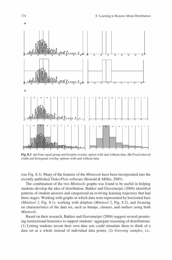
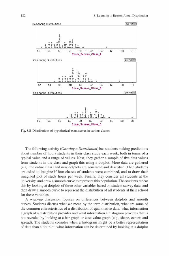
Next, in the Distinguishing Distributions activity, students are given a series ofdotplots that depict the distributions of hypothetical exam scores in various classes.For example, they are asked:

For classes A, B, and C, what is the main characteristic that distinguishes these three graphsfrom each other? What might explain this difference? (Fig. 8.8)

Each set of graphs reveals a different characteristic of distribution: e.g., center,spread, shape, and outliers. Students are then asked what features are importantto examine when describing distributions, what to look for, features that are alwayspresent such as shape, center and spread, and ones that might be present or absent,depending on the data set.


Fig. 8.8 Distributions of hypothetical exam scores in various classes

The following activity (Growing a Distribution) has students making predictionsabout number of hours students in their class study each week, both in terms of atypical value and a range of values. Next, they gather a sample of five data valuesfrom students in the class and graph this using a dotplot. More data are gathered(e.g., the entire class) and new dotplots are generated and described. Then studentsare asked to imagine if four classes of students were combined, and to draw theirimagined plot of study hours per week. Finally, they consider all students at theuniversity, and draw a smooth curve to represent this population. The students repeatthis by looking at dotplots of three other variables based on student survey data, andthen draw a smooth curve to represent the distribution of all students at their schoolfor these variables.

A wrap-up discussion focuses on differences between dotplots and smoothcurves. Students discuss what we mean by the term distribution, what are some ofthe common characteristics of a distribution of quantitative data, what informationa graph of a distribution provides and what information a histogram provides that isnot revealed by looking at a bar graph or case value graph (e.g., shape, center, andspread). The students consider when a histogram might be a better representationof data than a dot plot, what information can be determined by looking at a dotplot

Lesson 2: Exploring and Sorting Distributions 183

more easily than in a histogram, and what information is lost or not shown by ahistogram.

Lesson 2: Exploring and Sorting Distributions

This lesson begins with a data set of body measurements gathered from a set ofstudents that includes kneeling heights. After students make some predictions aboutthis variable, they examine and describe a dotplot of class data on kneeling heights.The students are led through a transformation of this dot plot into a histogram, usingTinkerPlots software. They compare different representations of the same data to seehow different features are hidden or revealed in different types of graphs.

In the third activity, students sort a set of histograms into different piles accord-ing to general shape, which leads students to recognize and label typical shapes,guiding them to see these distributions as entities, rather than as sets of individualvalues. The students further develop the idea of shape by changing bin widths onhistograms using Fathom software to manipulate and reveal how the size of the binsused affects the stability of the shape. In the fifth and final activity, students matchhistograms to variable descriptions, reasoning about the connections between visualcharacteristics of distributions and variable contexts.

Student learning goals for this lesson include:

1. To understand how a distribution is represented by a histogram and that a his-togram (or dotplot) allows us to describe shape, center, and spread of a quantita-tive variable in contrast to a bar graph (bar chart).

2. To understand the differences between case value graphs, bar graphs (case-valuebars) of individual data values and graphs displaying distributions of data suchas histograms.

3. To understand how graphical representations of data reveal the variability andshape of a data set.

4. To recognize and label typical shapes of distribution, using common statisticalterms (normal, skewed, bimodal, and uniform).

5. To understand that the shape of a graph may seem different depending on thegraphing technique used, so it may be important to manipulate a graph to seewhat the shape seems to be.

Description of the Lesson

In the What is a Histogram activity, students begin by making conjectures aboutwhat they would expect to see in the distribution of kneeling height data. This dataset is then used to help students develop an understanding of a histogram, by usingTinkerPlots to sort the data into sequential intervals, and then fuse the intervalsinto bars.


Fig. 8.9 Kneeling heights scattered dots in TinkerPlots

They begin with a graph of the data values, scattered as shown in Fig. 8.9, andafter playing with and examining the data, are guided to arrange the dots into case-value bars, to sort the smaller values of kneeling heights as shown in Fig. 8.10.

Students are then guided to use the Separate operation in TinkerPlots to separatethe cases into intervals that are then fused into a histogram, as shown in Figs. 8.11and 8.12.

In the Stretching Histograms activity, students use a histogram applet to ex-amine the effect of bin width on shape, seeing that larger and smaller bin widthsmay obscure shape and details (such as gaps, clusters, and outliers). Students arethen encouraged to think about the difference between the different types of plotsthey have seen (Exploring Different Representations of Data activity). These plots

Fig. 8.10 A case-value graph ordered by kneeling heights

Lesson 2: Exploring and Sorting Distributions 185

Fig. 8.11 Stacked kneeling height data with frequencies noted in each interval

include the dotplot, the case-value graph (value bar graph), and the histogram. Theyare then asked to consider which graphs help them better estimate the lowest fivevalues, where “most” of the kneeling heights are clustered, the middle or typicalvalue of kneeling heights, the spread, and the shape of the data. Students discusshow to determine the best representation to answer a particular question and whyone representation may be better than another.

In the next activity (Sorting Histogram), students work in small groups to sorta set of 21 different graphs, representing different data sets. Students sort the stackof graphs into piles, according to those that look the same or similar, then describewhat is similar about the graphs in each group, pick one representative graph for

Fig. 8.12 A histogram presenting the kneeling height in seven bins


each group, and come up with their own term to describe the general shape of eachgroup. A whole class discussion follows where group results are compared and thenthe correct statistical terms for the graphs (uniform, normal, right- and left-skewed,bimodal) can be introduced or reinforced. Models (uniform, normal) are describedin terms of symmetry and shape (bell-shape or rectangular). Other distributions thatdo not fit these models can be described in terms of their characteristics (skewness,bimodality or unimodality, etc.). A discussion of which descriptors can and cannotgo together may follow. For example, normal and skewed cannot go together.

During this discussion, some important points are addressed:

� Ideal shapes: density curves vs. histograms (theoretical vs. empirical distribu-tions)

� Different versions of ideal shapes� Idea of models, characteristics of distributions� Statistical words vs. informal descriptors� Other ways to describe a distribution� Why is it important to describe a distribution?� Normal, skewed, uniform, bimodal, and symmetric: which can be used together?

How well do they fit the graphs? Which fit best?

Next, students work in groups to discuss and sketch what they expect for the generalshape for some new data sets, and use the statistical terms to describe the shape ofeach. For example, the salaries of all persons employed at the University or gradeson an easy test. There is another whole class discussion to compare answers andexplanations.

The final activity (Matching Histograms to Variable Descriptions) has studentsmatch descriptions of variables to graphs of distributions, helping to develop stu-dents’ reasoning about behavior of data in different contexts and how this is relatedto different types of shapes of graphs. A wrap-up discussion focuses on the charac-teristics of distributions and how they are revealed in different types of graphs.

Summary

Understanding the idea of distribution is an important first step for students whowill encounter distributions of data and later distributions of sample statistics asthey proceed through their statistics course. While most textbooks ask students tolook at a histogram or stem plot and describe the shape, center, and spread, manystudents never understand the idea of distribution as an entity with characteristicsthat reveal important aspects of the variation of the data. The focus of the activitiesdescribed in this chapter is on developing a conceptual understanding of distribu-tion, and we have not included activities where students learn to construct differentgraphs, a topic well covered in most textbooks. We encourage instructors to repeat-edly have students interpret and describe distributions as they move through thecourse, whether plots of sample data or distributions of sample statistics.

chapter8 learning to reason about distributionreed/instructors/math 10041... · 166 8 learning to...

Documents