chapter6 combinatorialmotionplanning - university of illinoisplanning.cs.uiuc.edu/ch6.pdf ·...
TRANSCRIPT
Chapter 6
Combinatorial Motion Planning
Steven M. LaValle
University of Illinois
Copyright Steven M. LaValle 2006
Available for downloading at http://planning.cs.uiuc.edu/
Published by Cambridge University Press

Chapter 6
Combinatorial Motion Planning
Combinatorial approaches to motion planning find paths through the continuousconfiguration space without resorting to approximations. Due to this property,they are alternatively referred to as exact algorithms. This is in contrast to thesampling-based motion planning algorithms from Chapter 5.
6.1 Introduction
All of the algorithms presented in this chapter are complete, which means thatfor any problem instance (over the space of problems for which the algorithm isdesigned), the algorithm will either find a solution or will correctly report that nosolution exists. By contrast, in the case of sampling-based planning algorithms,weaker notions of completeness were tolerated: resolution completeness and prob-abilistic completeness.
Representation is important When studying combinatorial motion planningalgorithms, it is important to carefully consider the definition of the input. Whatis the representation used for the robot and obstacles? What set of transforma-tions may be applied to the robot? What is the dimension of the world? Arethe robot and obstacles convex? Are they piecewise linear? The specification ofpossible inputs defines a set of problem instances on which the algorithm will op-erate. If the instances have certain convenient properties (e.g., low dimensionality,convex models), then a combinatorial algorithm may provide an elegant, practicalsolution. If the set of instances is too broad, then a requirement of both complete-ness and practical solutions may be unreasonable. Many general formulations ofgeneral motion planning problems are PSPACE-hard1; therefore, such a hope ap-pears unattainable. Nevertheless, there exist general, complete motion planningalgorithms. Note that focusing on the representation is the opposite philosophyfrom sampling-based planning, which hides these issues in the collision detectionmodule.
1This implies NP-hard. An overview of such complexity statements appears in Section 6.5.1.
249
250 S. M. LaValle: Planning Algorithms
Reasons to study combinatorial methods There are generally two goodreasons to study combinatorial approaches to motion planning:
1. In many applications, one may only be interested in a special class of plan-ning problems. For example, the world might be 2D, and the robot mightonly be capable of translation. For many special classes, elegant and ef-ficient algorithms can be developed. These algorithms are complete, donot depend on approximation, and can offer much better performance thansampling-based planning methods, such as those in Chapter 5.
2. It is both interesting and satisfying to know that there are complete algo-rithms for an extremely broad class of motion planning problems. Thus,even if the class of interest does not have some special limiting assumptions,there still exist general-purpose tools and algorithms that can solve it. Thesealgorithms also provide theoretical upper bounds on the time needed to solvemotion planning problems.
Warning: Some methods are impractical Be careful not to make the wrongassumptions when studying the algorithms of this chapter. A few of them are ef-ficient and easy to implement, but many might be neither. Even if an algorithmhas an amazing asymptotic running time, it might be close to impossible to im-plement. For example, one of the most famous algorithms from computationalgeometry can split a simple2 polygon into triangles in O(n) time for a polygonwith n edges [19]. This is so amazing that it was covered in the New York Times,but the algorithm is so complicated that it is doubtful that anyone will ever imple-ment it. Sometimes it is preferable to use an algorithm that has worse theoreticalrunning time but is much easier to understand and implement. In general, though,it is valuable to understand both kinds of methods and decide on the trade-offsfor yourself. It is also an interesting intellectual pursuit to try to determine howefficiently a problem can be solved, even if the result is mainly of theoretical in-terest. This might motivate others to look for simpler algorithms that have thesame or similar asymptotic running times.
Roadmaps Virtually all combinatorial motion planning approaches construct aroadmap along the way to solving queries. This notion was introduced in Section5.6, but in this chapter stricter requirements are imposed in the roadmap definitionbecause any algorithm that constructs one needs to be complete. Some of thealgorithms in this chapter first construct a cell decomposition of Cfree from whichthe roadmap is consequently derived. Other methods directly construct a roadmapwithout the consideration of cells.
Let G be a topological graph (defined in Example 4.6) that maps into Cfree.Furthermore, let S ⊂ Cfree be the swath, which is set of all points reached by G,
2A polygonal region that has no holes.

6.2. POLYGONAL OBSTACLE REGIONS 251
as defined in (5.40). The graph G is called a roadmap if it satisfies two importantconditions:
1. Accessibility: From any q ∈ Cfree, it is simple and efficient to compute apath τ : [0, 1] → Cfree such that τ(0) = q and τ(1) = s, in which s may beany point in S. Usually, s is the closest point to q, assuming C is a metricspace.
2. Connectivity-preserving: Using the first condition, it is always possibleto connect some qI and qG to some s1 and s2, respectively, in S. The secondcondition requires that if there exists a path τ : [0, 1] → Cfree such thatτ(0) = qI and τ(1) = qG, then there also exists a path τ ′ : [0, 1] → S, suchthat τ ′(0) = s1 and τ
′(1) = s2. Thus, solutions are not missed because G failsto capture the connectivity of Cfree. This ensures that complete algorithmsare developed.
By satisfying these properties, a roadmap provides a discrete representation ofthe continuous motion planning problem without losing any of the original con-nectivity information needed to solve it. A query, (qI , qG), is solved by connectingeach query point to the roadmap and then performing a discrete graph search onG. To maintain completeness, the first condition ensures that any query can beconnected to G, and the second condition ensures that the search always succeedsif a solution exists.
6.2 Polygonal Obstacle Regions
Rather than diving into the most general forms of combinatorial motion plan-ning, it is helpful to first see several methods explained for a case that is easy tovisualize. Several elegant, straightforward algorithms exist for the case in whichC = R2 and Cobs is polygonal. Most of these cannot be directly extended to higherdimensions; however, some of the general principles remain the same. Therefore,it is very instructive to see how combinatorial motion planning approaches work intwo dimensions. There are also applications where these algorithms may directlyapply. One example is planning for a small mobile robot that may be modeled asa point moving in a building that can be modeled with a 2D polygonal floor plan.
After covering representations in Section 6.2.1, Sections 6.2.2–6.2.4 presentthree different algorithms to solve the same problem. The one in Section 6.2.2first performs cell decomposition on the way to building the roadmap, and theones in Sections 6.2.3 and 6.2.4 directly produce a roadmap. The algorithm inSection 6.2.3 computes maximum clearance paths, and the one in Section 6.2.4computes shortest paths (which consequently have no clearance).
252 S. M. LaValle: Planning Algorithms
Figure 6.1: A polygonal model specified by four oriented simple polygons.
6.2.1 Representation
Assume that W = R2; the obstacles, O, are polygonal; and the robot, A, is apolygonal body that is only capable of translation. Under these assumptions, Cobswill be polygonal. For the special case in which A is a point inW , O maps directlyto Cobs without any distortion. Thus, the problems considered in this section mayalso be considered as planning for a point robot. If A is not a point robot, thenthe Minkowski difference, (4.37), of O and A must be computed. For the casein which both A and each component of O are convex, the algorithm in Section4.3.2 can be applied to compute each component of Cobs. In general, both A andO may be nonconvex. They may even contain holes, which results in a Cobs modelsuch as that shown in Figure 6.1. In this case, A and O may be decomposedinto convex components, and the Minkowski difference can be computed for eachpair of components. The decompositions into convex components can actually beperformed by adapting the cell decomposition algorithm that will be presentedin Section 6.2.2. Once the Minkowski differences have been computed, they needto be merged to obtain a representation that can be specified in terms of simplepolygons, such as those in Figure 6.1. An efficient algorithm to perform thismerging is given in Section 2.4 of [28]. It can also be based on many of the sameprinciples as the planning algorithm in Section 6.2.2.
To implement the algorithms described in this section, it will be helpful tohave a data structure that allows convenient access to the information contained
6.2. POLYGONAL OBSTACLE REGIONS 253
in a model such as Figure 6.1. How is the outer boundary represented? How areholes inside of obstacles represented? How do we know which holes are insideof which obstacles? These questions can be efficiently answered by using thedoubly connected edge list data structure, which was described in Section 3.1.3for consistent labeling of polyhedral faces. We will need to represent models, suchas the one in Figure 6.1, and any other information that planning algorithms needto maintain during execution. There are three different records:
Vertices: Every vertex v contains a pointer to a point (x, y) ∈ C = R2 anda pointer to some half-edge that has v as its origin.
Faces: Every face has one pointer to a half-edge on the boundary thatsurrounds the face; the pointer value is nil if the face is the outermostboundary. The face also contains a list of pointers for each connected com-ponent (i.e., hole) that is contained inside of that face. Each pointer in thelist points to a half-edge of the component’s boundary.
Half-edges: Each half-edge is directed so that the obstacle portion is alwaysto its left. It contains five different pointers. There is a pointer to its originvertex. There is a twin half-edge pointer, which may point to a half-edge thatruns in the opposite direction (see Section 3.1.3). If the half-edge borders anobstacle, then this pointer is nil. Half-edges are always arranged in circularchains to form the boundary of a face. Such chains are oriented so that theobstacle portion (or a twin half-edge) is always to its left. Each half-edgestores a pointer to its internal face. It also contains pointers to the next andprevious half-edges in the circular chain of half-edges.
For the example in Figure 6.1, there are four circular chains of half-edges thateach bound a different face. The face record of the small triangular hole pointsto the obstacle face that contains the hole. Each obstacle contains a pointerto the face represented by the outermost boundary. By consistently assigningorientations to the half-edges, circular chains that bound an obstacle always runcounterclockwise, and chains that bound holes run clockwise. There are no twinhalf-edges because all half-edges bound part of Cobs. The doubly connected edgelist data structure is general enough to allow extra edges to be inserted that slicethrough Cfree. These edges will not be on the border of Cobs, but they can bemanaged using twin half-edge pointers. This will be useful for the algorithm inSection 6.2.2.
6.2.2 Vertical Cell Decomposition
Cell decompositions will be defined formally in Section 6.3, but here we use thenotion informally. Combinatorial methods must construct a finite data structurethat exactly encodes the planning problem. Cell decomposition algorithms achieve
254 S. M. LaValle: Planning Algorithms
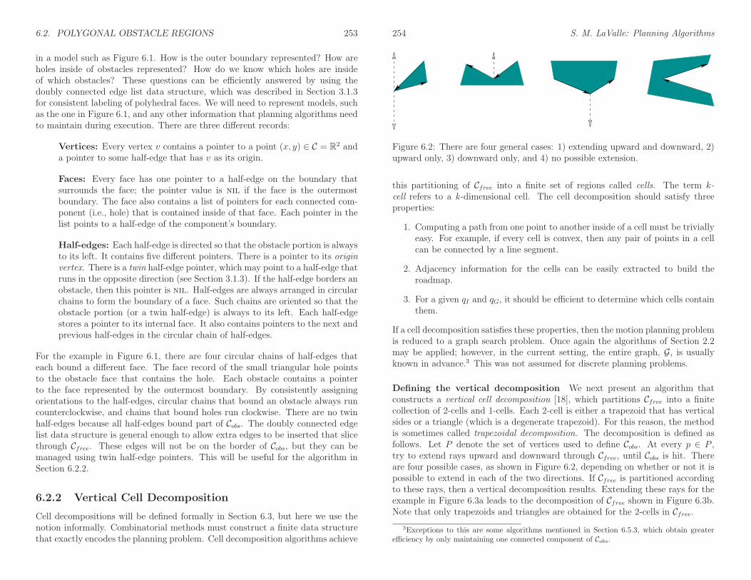
Figure 6.2: There are four general cases: 1) extending upward and downward, 2)upward only, 3) downward only, and 4) no possible extension.
this partitioning of Cfree into a finite set of regions called cells. The term k-cell refers to a k-dimensional cell. The cell decomposition should satisfy threeproperties:
1. Computing a path from one point to another inside of a cell must be triviallyeasy. For example, if every cell is convex, then any pair of points in a cellcan be connected by a line segment.
2. Adjacency information for the cells can be easily extracted to build theroadmap.
3. For a given qI and qG, it should be efficient to determine which cells containthem.
If a cell decomposition satisfies these properties, then the motion planning problemis reduced to a graph search problem. Once again the algorithms of Section 2.2may be applied; however, in the current setting, the entire graph, G, is usuallyknown in advance.3 This was not assumed for discrete planning problems.
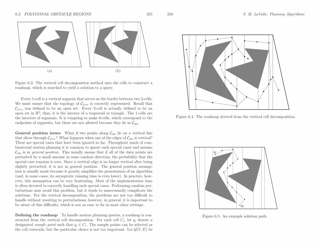
Defining the vertical decomposition We next present an algorithm thatconstructs a vertical cell decomposition [18], which partitions Cfree into a finitecollection of 2-cells and 1-cells. Each 2-cell is either a trapezoid that has verticalsides or a triangle (which is a degenerate trapezoid). For this reason, the methodis sometimes called trapezoidal decomposition. The decomposition is defined asfollows. Let P denote the set of vertices used to define Cobs. At every p ∈ P ,try to extend rays upward and downward through Cfree, until Cobs is hit. Thereare four possible cases, as shown in Figure 6.2, depending on whether or not it ispossible to extend in each of the two directions. If Cfree is partitioned accordingto these rays, then a vertical decomposition results. Extending these rays for theexample in Figure 6.3a leads to the decomposition of Cfree shown in Figure 6.3b.Note that only trapezoids and triangles are obtained for the 2-cells in Cfree.
3Exceptions to this are some algorithms mentioned in Section 6.5.3, which obtain greaterefficiency by only maintaining one connected component of Cobs.
6.2. POLYGONAL OBSTACLE REGIONS 255
(a) (b)
Figure 6.3: The vertical cell decomposition method uses the cells to construct aroadmap, which is searched to yield a solution to a query.
Every 1-cell is a vertical segment that serves as the border between two 2-cells.We must ensure that the topology of Cfree is correctly represented. Recall thatCfree was defined to be an open set. Every 2-cell is actually defined to be anopen set in R2; thus, it is the interior of a trapezoid or triangle. The 1-cells arethe interiors of segments. It is tempting to make 0-cells, which correspond to theendpoints of segments, but these are not allowed because they lie in Cobs.
General position issues What if two points along Cobs lie on a vertical linethat slices through Cfree? What happens when one of the edges of Cobs is vertical?These are special cases that have been ignored so far. Throughout much of com-binatorial motion planning it is common to ignore such special cases and assumeCobs is in general position. This usually means that if all of the data points areperturbed by a small amount in some random direction, the probability that thespecial case remains is zero. Since a vertical edge is no longer vertical after beingslightly perturbed, it is not in general position. The general position assump-tion is usually made because it greatly simplifies the presentation of an algorithm(and, in some cases, its asymptotic running time is even lower). In practice, how-ever, this assumption can be very frustrating. Most of the implementation timeis often devoted to correctly handling such special cases. Performing random per-turbations may avoid this problem, but it tends to unnecessarily complicate thesolutions. For the vertical decomposition, the problems are not too difficult tohandle without resorting to perturbations; however, in general, it is important tobe aware of this difficulty, which is not as easy to fix in most other settings.
Defining the roadmap To handle motion planning queries, a roadmap is con-structed from the vertical cell decomposition. For each cell Ci, let qi denote adesignated sample point such that qi ∈ Ci. The sample points can be selected asthe cell centroids, but the particular choice is not too important. Let G(V,E) be
256 S. M. LaValle: Planning Algorithms
Figure 6.4: The roadmap derived from the vertical cell decomposition.
qI
qG
Figure 6.5: An example solution path.

6.2. POLYGONAL OBSTACLE REGIONS 257
a topological graph defined as follows. For every cell, Ci, define a vertex qi ∈ V .There is a vertex for every 1-cell and every 2-cell. For each 2-cell, define an edgefrom its sample point to the sample point of every 1-cell that lies along its bound-ary. Each edge is a line-segment path between the sample points of the cells. Theresulting graph is a roadmap, as depicted in Figure 6.4. The accessibility condi-tion is satisfied because every sample point can be reached by a straight-line paththanks to the convexity of every cell. The connectivity condition is also satisfiedbecause G is derived directly from the cell decomposition, which also preservesthe connectivity of Cfree. Once the roadmap is constructed, the cell informationis no longer needed for answering planning queries.
Solving a query Once the roadmap is obtained, it is straightforward to solvea motion planning query, (qI , qG). Let C0 and Ck denote the cells that contain qIand qG, respectively. In the graph G, search for a path that connects the samplepoint of C0 to the sample point of Ck. If no such path exists, then the planningalgorithm correctly declares that no solution exists. If one does exist, then let C1,C2, . . ., Ck−1 denote the sequence of 1-cells and 2-cells visited along the computedpath in G from C0 to Ck.
A solution path can be formed by simply “connecting the dots.” Let q0, q1, q2,. . ., qk−1, qk, denote the sample points along the path in G. There is one samplepoint for every cell that is crossed. The solution path, τ : [0, 1] → Cfree, is formedby setting τ(0) = qI , τ(1) = qG, and visiting each of the points in the sequencefrom q0 to qk by traveling along the shortest path. For the example, this leads tothe solution shown in Figure 6.5. In selecting the sample points, it was importantto ensure that each path segment from the sample point of one cell to the samplepoint of its neighboring cell is collision-free.4
Computing the decomposition The problem of efficiently computing the de-composition has not yet been considered. Without concern for efficiency, theproblem appears simple enough that all of the required steps can be computed bybrute-force computations. If Cobs has n vertices, then this approach would take atleast O(n2) time because intersection tests have to be made between each verticalray and each segment. This even ignores the data structure issues involved infinding the cells that contain the query points and in building the roadmap thatholds the connectivity information. By careful organization of the computation,it turns out that all of this can be nicely handled, and the resulting running timeis only O(n lg n).
Plane-sweep principle The algorithm is based on the plane-sweep (or line-sweep) principle from computational geometry [12, 28, 29], which forms the basis
4This is the reason why the approach is defined differently from Chapter 1 of [47]. In thatcase, sample points were not placed in the interiors of the 2-cells, and collision could result forsome queries.
258 S. M. LaValle: Planning Algorithms
of many combinatorial motion planning algorithms and many other algorithms ingeneral. Much of computational geometry can be considered as the developmentof data structures and algorithms that generalize the sorting problem to multipledimensions. In other words, the algorithms carefully “sort” geometric information.
The word “sweep” is used to refer to these algorithms because it can be imag-ined that a line (or plane, etc.) sweeps across the space, only to stop where somecritical change occurs in the information. This gives the intuition, but the sweep-ing line is not explicitly represented by the algorithm. To construct the verticaldecomposition, imagine that a vertical line sweeps from x = −∞ to x = ∞, using(x, y) to denote a point in C = R2.
From Section 6.2.1, note that the set P of Cobs vertices are the only data in R2
that appear in the problem input. It therefore seems reasonable that interestingthings can only occur at these points. Sort the points in P in increasing order bytheir X coordinate. Assuming general position, no two points have the same Xcoordinate. The points in P will now be visited in order of increasing x value.Each visit to a point will be referred to as an event. Before, after, and in betweenevery event, a list, L, of some Cobs edges will be maintained. This list must bemaintained at all times in the order that the edges appear when stabbed by thevertical sweep line. The ordering is maintained from lower to higher.
Algorithm execution Figures 6.6 and 6.7 show how the algorithm proceeds.Initially, L is empty, and a doubly connected edge list is used to represent Cfree.Each connected component of Cfree yields a single face in the data structure.Suppose inductively that after several events occur, L is correctly maintained.For each event, one of the four cases in Figure 6.2 occurs. By maintaining L in abalanced binary search tree [24], the edges above and below p can be determinedin O(lg n) time. This is much better than O(n) time, which would arise fromchecking every segment. Depending on which of the four cases from Figure 6.2occurs, different updates to L are made. If the first case occurs, then two differentedges are inserted, and the face of which p is on the border is split two timesby vertical line segments. For each of the two vertical line segments, two half-edges are added, and all faces and half-edges must be updated correctly (thisoperation is local in that only records adjacent to where the change occurs needto be updated). The next two cases in Figure 6.2 are simpler; only a single facesplit is made. For the final case, no splitting occurs.
Once the face splitting operations have been performed, L needs to be updated.When the sweep line crosses p, two edges are always affected. For example, inthe first and last cases of Figure 6.2, two edges must be inserted into L (themirror images of these cases cause two edges to be deleted from L). If the middletwo cases occur, then one edge is replaced by another in L. These insertion anddeletion operations can be performed in O(lg n) time. Since there are n events,the running time for the construction algorithm is O(n lg n).
The roadmap G can be computed from the face pointers of the doubly con-

6.2. POLYGONAL OBSTACLE REGIONS 259
1 2 3 4 5 6 7 8 9 10 11 12 130
a
d
f
b
i
m
nh
gc
e
l
j
k
Figure 6.6: There are 14 events in this example.
Event Sorted Edges in L Event Sorted Edges in L0 a, b 7 d, j, n, b1 d, b 8 d, j, n,m, l, b2 d, f, e, b 9 d, j, l, b3 d, f, i, b 10 d, k, l, b4 d, f, g, h, i, b 11 d, b5 d, f, g, j, n, h, i, b 12 d, c6 d, f, g, j, n, b 13
Figure 6.7: The status of L is shown after each of 14 events occurs. Before thefirst event, L is empty.
260 S. M. LaValle: Planning Algorithms
One closestpoint
Two closestpoints
One closestpoint
Figure 6.8: The maximum clearance roadmap keeps as far away from the Cobs aspossible. This involves traveling along points that are equidistant from two ormore points on the boundary of Cobs.
Edge-Edge Vertex-Vertex Vertex-Edge
Figure 6.9: Voronoi roadmap pieces are generated in one of three possible cases.The third case leads to a quadratic curve.
nected edge list. A more elegant approach is to incrementally build G at eachevent. In fact, all of the pointer maintenance required to obtain a consistent dou-bly connected edge list can be ignored if desired, as long as G is correctly builtand the sample point is obtained for each cell along the way. We can even goone step further, by forgetting about the cell decomposition and directly buildinga topological graph of line-segment paths between all sample points of adjacentcells.
6.2.3 Maximum-Clearance Roadmaps
A maximum-clearance roadmap tries to keep as far as possible from Cobs, as shownfor the corridor in Figure 6.8. The resulting solution paths are sometimes pre-ferred in mobile robotics applications because it is difficult to measure and controlthe precise position of a mobile robot. Traveling along the maximum-clearanceroadmap reduces the chances of collisions due to these uncertainties. Other namesfor this roadmap are generalized Voronoi diagram and retraction method [60]. It isconsidered as a generalization of the Voronoi diagram (recall from Section 5.2.2)from the case of points to the case of polygons. Each point along a roadmap edgeis equidistant from two points on the boundary of Cobs. Each roadmap vertex
6.2. POLYGONAL OBSTACLE REGIONS 261
corresponds to the intersection of two or more roadmap edges and is thereforeequidistant from three or more points along the boundary of Cobs.
The retraction term comes from topology and provides a nice intuition aboutthe method. A subspace S is a deformation retract of a topological space X if thefollowing continuous homotopy, h : X × [0, 1] → X, can be defined as follows [35]:
1. h(x, 0) = x for all x ∈ X.
2. h(x, 1) is a continuous function that maps every element of X to some ele-ment of S.
3. For all t ∈ [0, 1], h(s, t) = s for any s ∈ S.
The intuition is that Cfree is gradually thinned through the homotopy process,until a skeleton, S, is obtained. An approximation to this shrinking process canbe imagined by shaving off a thin layer around the whole boundary of Cfree. Ifthis is repeated iteratively, the maximum-clearance roadmap is the only part thatremains (assuming that the shaving always stops when thin “slivers” are obtained).
To construct the maximum-clearance roadmap, the concept of features fromSection 5.3.3 is used again. Let the feature set refer to the set of all edges andvertices of Cobs. Candidate paths for the roadmap are produced by every pairof features. This leads to a naive O(n4) time algorithm as follows. For everyedge-edge feature pair, generate a line as shown in Figure 6.9a. For every vertex-vertex pair, generate a line as shown in Figure 6.9b. The maximum-clearancepath between a point and a line is a parabola. Thus, for every edge-point pair,generate a parabolic curve as shown in Figure 6.9c. The portions of the paths thatactually lie on the maximum-clearance roadmap are determined by intersectingthe curves. Several algorithms exist that provide better asymptotic running times[48, 50], but they are considerably more difficult to implement. The best-knownalgorithm runs in O(n lg n) time in which n is the number of roadmap curves [71].
6.2.4 Shortest-Path Roadmaps
Instead of generating paths that maximize clearance, suppose that the goal is tofind shortest paths. This leads to the shortest-path roadmap, which is also calledthe reduced visibility graph in [47]. The idea was first introduced in [58] and mayperhaps be the first example of a motion planning algorithm. The shortest-pathroadmap is in direct conflict with maximum clearance because shortest paths tendto graze the corners of Cobs. In fact, the problem is ill posed because Cfree is anopen set. For any path τ : [0, 1] → Cfree, it is always possible to find a shorterone. For this reason, we must consider the problem of determining shortest pathsin cl(Cfree), the closure of Cfree. This means that the robot is allowed to “touch”or “graze” the obstacles, but it is not allowed to penetrate them. To actuallyuse the computed paths as solutions to a motion planning problem, they needto be slightly adjusted so that they come very close to Cobs but do not make
262 S. M. LaValle: Planning Algorithms
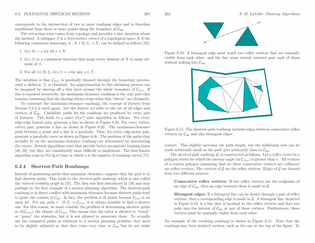
Figure 6.10: A bitangent edge must touch two reflex vertices that are mutuallyvisible from each other, and the line must extend outward past each of themwithout poking into Cobs.
Figure 6.11: The shortest-path roadmap includes edges between consecutive reflexvertices on Cobs and also bitangent edges.
contact. This slightly increases the path length, but the additional cost can bemade arbitrarily small as the path gets arbitrarily close to Cobs.
The shortest-path roadmap, G, is constructed as follows. Let a reflex vertex be apolygon vertex for which the interior angle (in Cfree) is greater than π. All verticesof a convex polygon (assuming that no three consecutive vertices are collinear)are reflex vertices. The vertices of G are the reflex vertices. Edges of G are formedfrom two different sources:
Consecutive reflex vertices: If two reflex vertices are the endpoints ofan edge of Cobs, then an edge between them is made in G.
Bitangent edges: If a bitangent line can be drawn through a pair of reflexvertices, then a corresponding edge is made in G. A bitangent line, depictedin Figure 6.10, is a line that is incident to two reflex vertices and does notpoke into the interior of Cobs at any of these vertices. Furthermore, thesevertices must be mutually visible from each other.
An example of the resulting roadmap is shown in Figure 6.11. Note that theroadmap may have isolated vertices, such as the one at the top of the figure. To

6.2. POLYGONAL OBSTACLE REGIONS 263
qG
qI
Figure 6.12: To solve a query, qI and qG are connected to all visible roadmapvertices, and graph search is performed.
qG
qI
Figure 6.13: The shortest path in the extended roadmap is the shortest pathbetween qI and qG.
solve a query, qI and qG are connected to all roadmap vertices that are visible;this is shown in Figure 6.12. This makes an extended roadmap that is searchedfor a solution. If Dijkstra’s algorithm is used, and if each edge is given a cost thatcorresponds to its path length, then the resulting solution path is the shortestpath between qI and qG. The shortest path for the example in Figure 6.12 isshown in Figure 6.13.
If the bitangent tests are performed naively, then the resulting algorithm re-quires O(n3) time, in which n is the number of vertices of Cobs. There are O(n2)pairs of reflex vertices that need to be checked, and each check requires O(n) timeto make certain that no other edges prevent their mutual visibility. The plane-sweep principle from Section 6.2.2 can be adapted to obtain a better algorithm,which takes only O(n2 lg n) time. The idea is to perform a radial sweep from each
264 S. M. LaValle: Planning Algorithms
p1 p3
p4p6
p5
p2
Figure 6.14: Potential bitangents can be identified by checking for left turns,which avoids the use of trigonometric functions and their associated numericalproblems.
reflex vertex, v. A ray is started at θ = 0, and events occur when the ray touchesvertices. A set of bitangents through v can be computed in this way in O(n lg n)time. Since there are O(n) reflex vertices, the total running time is O(n2 lg n). SeeChapter 15 of [28] for more details. There exists an algorithm that can computethe shortest-path roadmap in time O(n lg n+m), in which m is the total numberof edges in the roadmap [30]. If the obstacle region is described by a simple poly-gon, the time complexity can be reduced to O(n); see [56] for many shortest-pathvariations and references.
To improve numerical robustness, the shortest-path roadmap can be imple-mented without the use of trigonometric functions. For a sequence of three points,p1, p2, p3, define the left-turn predicate, fl : R
2 × R2 × R2 → true, false, asfl(p1, p2, p3) = true if and only if p3 is to the left of the ray that starts at p1 andpierces p2. A point p2 is a reflex vertex if and only if fl(p1, p2, p3) = true, in whichp1 and p3 are the points before and after, respectively, along the boundary of Cobs.The bitangent test can be performed by assigning points as shown in Figure 6.14.Assume that no three points are collinear and the segment that connects p2 andp5 is not in collision. The pair, p2, p5, of vertices should receive a bitangent edgeif the following sentence is false:
(
fl(p1, p2, p5)⊕ fl(p3, p2, p5))
∨(
fl(p4, p5, p2)⊕ fl(p6, p5, p2))
, (6.1)
in which ⊕ denotes logical “exclusive or.” The fl predicate can be implementedwithout trigonometric functions by defining
M(p1, p2, p3) =
1 x1 y11 x2 y21 x3 y3
, (6.2)
in which pi = (xi, yi). If det(M) > 0, then fl(p1, p2, p3) = true; otherwise,fl(p1, p2, p3) = false.
6.3 Cell Decompositions
Section 6.2.2 introduced the vertical cell decomposition to solve the motion plan-ning problem when Cobs is polygonal. It is important to understand, however, that

6.3. CELL DECOMPOSITIONS 265
this is just one choice among many for the decomposition. Some of these choicesmay not be preferable in 2D; however, they might generalize better to higherdimensions. Therefore, other cell decompositions are covered in this section, toprovide a smoother transition from vertical cell decomposition to cylindrical alge-braic decomposition in Section 6.4, which solves the motion planning problem inany dimension for any semi-algebraic model. Along the way, a cylindrical decom-position will appear in Section 6.3.4 for the special case of a line-segment robotin W = R2.
6.3.1 General Definitions
In this section, the term complex refers to a collection of cells together with theirboundaries. A partition into cells can be derived from a complex, but the complexcontains additional information that describes how the cells must fit together. Theterm cell decomposition still refers to the partition of the space into cells, whichis derived from a complex.
It is tempting to define complexes and cell decompositions in a very generalmanner. Imagine that any partition of Cfree could be called a cell decomposition.A cell could be so complicated that the notion would be useless. Even Cfree itselfcould be declared as one big cell. It is more useful to build decompositions outof simpler cells, such as ones that contain no holes. Formally, this requires thatevery k-dimensional cell is homeomorphic to Bk ⊂ Rk, an open k-dimensionalunit ball. From a motion planning perspective, this still yields cells that are quitecomplicated, and it will be up to the particular cell decomposition method toenforce further constraints to yield a complete planning algorithm.
Two different complexes will be introduced. The simplicial complex is ex-plained because it is one of the easiest to understand. Although it is useful inmany applications, it is not powerful enough to represent all of the complexes thatarise in motion planning. Therefore, the singular complex is also introduced. Al-though it is more complicated to define, it encompasses all of the cell complexesthat are of interest in this book. It also provides an elegant way to representtopological spaces. Another important cell complex, which is not covered here, isthe CW-complex [34].
Simplicial Complex For this definition, it is assumed that X = Rn. Let p1, p2,. . ., pk+1, be k+1 linearly independent5 points in Rn. A k-simplex, [p1, . . . , pk+1],is formed from these points as
[p1, . . . , pk+1] =
k+1∑
i=1
αipi ∈ Rn∣
∣
∣ αi ≥ 0 for all i andk+1∑
i=1
αi = 1
, (6.3)
5Form k vectors by subtracting p1 from the other k points for some positive integer k suchthat k ≤ n. Arrange the vectors into a k × n matrix. For linear independence, there must beat least one k × k cofactor with a nonzero determinant. For example, if k = 2, then the threepoints cannot be collinear.
266 S. M. LaValle: Planning Algorithms
Not a simplicial complex A simplicial complex
Figure 6.15: To become a simplicial complex, the simplex faces must fit togethernicely.
in which αipi is the scalar multiplication of αi by each of the point coordinates.Another way to view (6.3) is as the convex hull of the k + 1 points (i.e., all waysto linearly interpolate between them). If k = 2, a triangular region is obtained.For k = 3, a tetrahedron is produced.
For any k-simplex and any i such that 1 ≤ i ≤ k + 1, let αi = 0. This yieldsa (k − 1)-dimensional simplex that is called a face of the original simplex. A 2-simplex has three faces, each of which is a 1-simplex that may be called an edge.Each 1-simplex (or edge) has two faces, which are 0-simplexes called vertices.
To form a complex, the simplexes must fit together in a nice way. This yieldsa high-dimensional notion of a triangulation, which in R2 is a tiling composedof triangular regions. A simplicial complex, K, is a finite set of simplexes thatsatisfies the following:
1. Any face of a simplex in K is also in K.
2. The intersection of any two simplexes in K is either a common face of bothof them or the intersection is empty.
Figure 6.15 illustrates these requirements. For k > 0, a k-cell of K is defined tobe interior, int([p1, . . . , pk+1]), of any k-simplex. For k = 0, every 0-simplex is a0-cell. The union of all of the cells forms a partition of the point set covered byK. This therefore provides a cell decomposition in a sense that is consistent withSection 6.2.2.
Singular complex Simplicial complexes are useful in applications such as ge-ometric modeling and computer graphics for computing the topology of models.Due to the complicated topological spaces, implicit, nonlinear models, and de-composition algorithms that arise in motion planning, they are insufficient for themost general problems. A singular complex is a generalization of the simplicialcomplex. Instead of being limited to Rn, a singular complex can be defined onany manifold, X (it can even be defined on any Hausdorff topological space). Themain difference is that, for a simplicial complex, each simplex is a subset of Rn;

6.3. CELL DECOMPOSITIONS 267
however, for a singular complex, each singular simplex is actually a homeomor-phism from a (simplicial) simplex in Rn to a subset of X.
To help understand the idea, first consider a 1D singular complex, which hap-pens to be a topological graph (as introduced in Example 4.6). The interval [0, 1]is a 1-simplex, and a continuous path τ : [0, 1] → X is a singular 1-simplex be-cause it is a homeomorphism of [0, 1] to the image of τ in X. Suppose G(V,E) isa topological graph. The cells are subsets of X that are defined as follows. Eachpoint v ∈ V is a 0-cell in X. To follow the formalism, each is considered as theimage of a function f : 0 → X, which makes it a singular 0-simplex, because0 is a 0-simplex. For each path τ ∈ E, the corresponding 1-cell is
x ∈ X | τ(s) = x for some s ∈ (0, 1). (6.4)
Expressed differently, it is τ((0, 1)), the image of the path τ , except that theendpoints are removed because they are already covered by the 0-cells (the cellsmust form a partition).
These principles will now be generalized to higher dimensions. Since all ballsand simplexes of the same dimension are homeomorphic, balls can be used insteadof a simplex in the definition of a singular simplex. Let Bk ⊂ Rk denote a closed,k-dimensional unit ball,
Dk = x ∈ Rn | ‖x‖ ≤ 1, (6.5)
in which ‖·‖ is the Euclidean norm. A singular k-simplex is a continuous mappingσ : Dk → X. Let int(Dk) refer to the interior of Dk. For k ≥ 1, the k-cell, C,corresponding to a singular k-simplex, σ, is the image C = σ(int(Dk)) ⊆ X.The 0-cells are obtained directly as the images of the 0 singular simplexes. Eachsingular 0-simplex maps to the 0-cell in X. If σ is restricted to int(Dk), then itactually defines a homeomorphism between Dk and C. Note that both of theseare open sets if k > 0.
A simplicial complex requires that the simplexes fit together nicely. The sameconcept is applied here, but topological concepts are used instead because theyare more general. Let K be a set of singular simplexes of varying dimensions. LetSk denote the union of the images of all singular i-simplexes for all i ≤ k.
A collection of singular simplexes that map into a topological space X is calleda singular complex if:
1. For each dimension k, the set Sk ⊆ X must be closed. This means that thecells must all fit together nicely.
2. Each k-cell is an open set in the topological subspace Sk. Note that 0-cellsare open in S0, even though they are usually closed in X.
Example 6.1 (Vertical Decomposition) The vertical decomposition of Sec-tion 6.2.2 is a nice example of a singular complex that is not a simplicial complex
268 S. M. LaValle: Planning Algorithms
because it contains trapezoids. The interior of each trapezoid and triangle formsa 2-cell, which is an open set. For every pair of adjacent 2-cells, there is a 1-cell ontheir common boundary. There are no 0-cells because the vertices lie in Cobs, notin Cfree. The subspace S2 is formed by taking the union of all 2-cells and 1-cellsto yield S2 = Cfree. This satisfies the closure requirement because the complexis built in Cfree only; hence, the topological space is Cfree. The set S2 = Cfree isboth open and closed. The set S1 is the union of all 1-cells. This is also closedbecause the 1-cell endpoints all lie in Cobs. Each 1-cell is also an open set.
One way to avoid some of these strange conclusions from the topology re-stricted to Cfree is to build the vertical decomposition in cl(Cfree), the closure ofCfree. This can be obtained by starting with the previously defined vertical de-composition and adding a new 1-cell for every edge of Cobs and a 0-cell for everyvertex of Cobs. Now S3 = cl(Cfree), which is closed in R2. Likewise, S2, S1, and S0,are closed in the usual way. Each of the individual k-dimensional cells, however,is open in the topological space Sk. The only strange case is that the 0-cells areconsidered open, but this is true in the discrete topological space S0.
6.3.2 2D Decompositions
The vertical decomposition method of Section 6.2.2 is just one choice of manycell decomposition methods for solving the problem when Cobs is polygonal. Itprovides a nice balance between the number of cells, computational efficiency,and implementation ease. It is usually possible to decompose Cobs into far fewerconvex cells. This would be preferable for multiple-query applications becausethe roadmap would be smaller. It is unfortunately quite difficult to optimize thenumber of cells. Determining the decomposition of a polygonal Cobs with holesthat uses the smallest number of convex cells is NP-hard [44, 52]. Therefore, weare willing to tolerate nonoptimal decompositions.
Triangulation One alternative to the vertical decomposition is to perform atriangulation, which yields a simplicial complex over Cfree. Figure 6.16 shows anexample. Since Cfree is an open set, there are no 0-cells. Each 2-simplex (triangle)has either one, two, or three faces, depending on how much of its boundary isshared with Cobs. A roadmap can be made by connecting the samples for 1-cellsand 2-cells as shown in Figure 6.17. Note that there are many ways to triangulateCfree for a given problem. Finding good triangulations, which for example meanstrying to avoid thin triangles, is given considerable attention in computationalgeometry [12, 28, 29].
How can the triangulation be computed? It might seem tempting to run thevertical decomposition algorithm of Section 6.2.2 and split each trapezoid intotwo triangles. Even though this leads to triangular cells, it does not produce asimplicial complex (two triangles could abut the same side of a triangle edge).

6.3. CELL DECOMPOSITIONS 269
Figure 6.16: A triangulation of Cfree.
Figure 6.17: A roadmap obtained from the triangulation.
270 S. M. LaValle: Planning Algorithms
A naive approach is to incrementally split faces by attempting to connect twovertices of a face by a line segment. If this segment does not intersect othersegments, then the split can be made. This process can be iteratively performedover all vertices of faces that have more than three vertices, until a triangulationis eventually obtained. Unfortunately, this results in an O(n3) time algorithmbecause O(n2) pairs must be checked in the worst case, and each check requiresO(n) time to determine whether an intersection occurs with other segments. Thiscan be easily reduced to O(n2 lg n) by performing radial sweeping. Chapter 3 of[28] presents an algorithm that runs in O(n lg n) time by first partitioning Cfreeintomonotone polygons, and then efficiently triangulating each monotone polygon.If Cfree is simply connected, then, surprisingly, a triangulation can be computedin linear time [19]. Unfortunately, this algorithm is too complicated to use inpractice (there are, however, simpler algorithms for which the complexity is closeto O(n); see [10] and the end of Chapter 3 of [28] for surveys).
Cylindrical decomposition The cylindrical decomposition is very similar tothe vertical decomposition, except that when any of the cases in Figure 6.2 occurs,then a vertical line slices through all faces, all the way from y = −∞ to y = ∞.The result is shown in Figure 6.18, which may be considered as a singular complex.This may appear very inefficient in comparison to the vertical decomposition;however, it is presented here because it generalizes nicely to any dimension, anyC-space topology, and any semi-algebraic model. Therefore, it is presented here toease the transition to more general decompositions. The most important propertyof the cylindrical decomposition is shown in Figure 6.19. Consider each verticalstrip between two events. When traversing a strip from y = −∞ to y = ∞,the points alternate between being Cobs and Cfree. For example, between events4 and 5, the points below edge f are in Cfree. Points between f and g lie inCobs. Points between g and h lie in Cfree, and so forth. The cell decompositioncan be defined so that 2D cells are also created in Cobs. Let S(x, y) denote thelogical predicate (3.6) from Section 3.1.1. When traversing a strip, the value ofS(x, y) also alternates. This behavior is the main reason to construct a cylindricaldecomposition, which will become clearer in Section 6.4.2. Each vertical strip isactually considered to be a cylinder, hence, the name cylindrical decomposition(i.e., there are not necessarily any cylinders in the 3D geometric sense).
6.3.3 3D Vertical Decomposition
It turns out that the vertical decomposition method of Section 6.2.2 can be ex-tended to any dimension by recursively applying the sweeping idea. The methodrequires, however, that Cobs is piecewise linear. In other words, Cobs is representedas a semi-algebraic model for which all primitives are linear. Unfortunately, mostof the general motion planning problems involve nonlinear algebraic primitivesbecause of the nonlinear transformations that arise from rotations. Recall the

6.3. CELL DECOMPOSITIONS 271
1 2 3 4 5 6 7 8 9 10 11 12 130
a
b
i
h
gc
e
l
f
j
k
nm
d
Figure 6.18: The cylindrical decomposition differs from the vertical decompositionin that the rays continue forever instead of stopping at the nearest edge. Comparethis figure to Figure 6.6.
1 2 3 4 5 6 7 8 9 10 11 12 130
a
b
i
h
gc
e
l
mn
d
k
f
j
Figure 6.19: The cylindrical decomposition produces vertical strips. Inside of astrip, there is a stack of collision-free cells, separated by Cobs.
272 S. M. LaValle: Planning Algorithms
y y y
z z z
y
z
x
Figure 6.20: In higher dimensions, the sweeping idea can be applied recursively.
complicated algebraic Cobs model constructed in Section 4.3.3. To handle genericalgebraic models, powerful techniques from computational algebraic geometry areneeded. This will be covered in Section 6.4.
One problem for which Cobs is piecewise linear is a polyhedral robot that cantranslate in R3, and the obstacles in W are polyhedra. Since the transformationequations are linear in this case, Cobs ⊂ R3 is polyhedral. The polygonal faces ofCobs are obtained by forming geometric primitives for each of the Type FV, TypeVF, and Type EE cases of contact between A and O, as mentioned in Section4.3.2.
Figure 6.20 illustrates the algorithm that constructs the 3D vertical decompo-sition. Compare this to the algorithm in Section 6.2.2. Let (x, y, z) denote a pointin C = R3. The vertical decomposition yields convex 3-cells, 2-cells, and 1-cells.Neglecting degeneracies, a generic 3-cell is bounded by six planes. The cross sec-tion of a 3-cell for some fixed x value yields a trapezoid or triangle, exactly as inthe 2D case, but in a plane parallel to the yz plane. Two sides of a generic 3-cellare parallel to the yz plane, and two other sides are parallel to the xz plane. The3-cell is bounded above and below by two polygonal faces of Cobs.
6.3. CELL DECOMPOSITIONS 273
Initially, sort the Cobs vertices by their x coordinate to obtain the events. Nowconsider sweeping a plane perpendicular to the x-axis. The plane for a fixed valueof x produces a 2D polygonal slice of Cobs. Three such slices are shown at thebottom of Figure 6.20. Each slice is parallel to the yz plane and appears to lookexactly like a problem that can be solved by the 2D vertical decomposition method.The 2-cells in a slice are actually slices of 3-cells in the 3D decomposition. Theonly places in which these 3-cells can critically change is when the sweeping planestops at some x value. The center slice in Figure 6.20 corresponds to the case inwhich a vertex of a convex polyhedron is encountered, and all of the polyhedronlies to right of the sweep plane (i.e., the rest of the polyhedron has not beenencountered yet). This corresponds to a place where a critical change must occurin the slices. These are 3D versions of the cases in Figure 6.2, which indicate howthe vertical decomposition needs to be updated. The algorithm proceeds by firstbuilding the 2D vertical decomposition at the first x event. At each event, the 2Dvertical decomposition must be updated to take into account the critical changes.During this process, the 3D cell decomposition and roadmap can be incrementallyconstructed, as in the 2D case.
The roadmap is constructed by placing a sample point in the center of each3-cell and 2-cell. The vertices are the sample points, and edges are added tothe roadmap by connecting the sample points for each case in which a 3-cell isadjacent to a 2-cell.
This same principle can be extended to any dimension, but the applicationsto motion planning are limited because the method requires linear models (or atleast it is very challenging to adapt to nonlinear models; in some special cases, thiscan be done). See [32] for a summary of the complexity of vertical decompositionsfor various geometric primitives and dimensions.
6.3.4 A Decomposition for a Line-Segment Robot
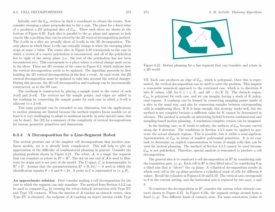
This section presents one of the simplest cell decompositions that involves non-linear models, yet it is already fairly complicated. This will help to give anappreciation of the difficulty of combinatorial planning in general. Consider theplanning problem shown in Figure 6.21. The robot, A, is a single line segmentthat can translate or rotate in W = R2. The dot on one end of A is used to illus-trate its origin and is not part of the model. The C-space, C, is homeomorphic toR2 × S1. Assume that the parameterization R2 × [0, 2π]/ ∼ is used in which theidentification equates θ = 0 and θ = 2π. A point in C is represented as (x, y, θ).
An approximate solution First consider making a cell decomposition for thecase in which the segment can only translate. The method from Section 4.3.2 canbe used to compute Cobs by treating the robot-obstacle interaction with Type EVand Type VE contacts. When the interior of A touches an obstacle vertex, thenType EV is obtained. An endpoint of A touching an object interior yields Type
274 S. M. LaValle: Planning Algorithms
Figure 6.21: Motion planning for a line segment that can translate and rotate ina 2D world.
VE. Each case produces an edge of Cobs, which is polygonal. Once this is repre-sented, the vertical decomposition can be used to solve the problem. This inspiresa reasonable numerical approach to the rotational case, which is to discretize θinto K values, i∆θ, for 0 ≤ i ≤ K, and ∆θ = 2π/K [3]. The obstacle region,Cobs, is polygonal for each case, and we can imagine having a stack of K polyg-onal regions. A roadmap can be formed by connecting sampling points inside ofa slice in the usual way, and also by connecting samples between correspondingcells in neighboring slices. If K is large enough, this strategy works well, but themethod is not complete because a sufficient value for K cannot be determined inadvance. The method is actually an interesting hybrid between combinatorial andsampling-based motion planning. A resolution-complete version can be imagined.
In the limiting case, as K tends to infinity, the surfaces of Cobs become curvedalong the θ direction. The conditions in Section 4.3.3 must be applied to gen-erate the actual obstacle regions. This is possible, but it yields a semi-algebraicrepresentation of Cobs in terms of implicit polynomial primitives. It is no easytask to determine an explicit representation in terms of simple cells that can beused for motion planning. The method of Section 6.3.3 cannot be used becauseCobs is not polyhedral. Therefore, special analysis is warranted to produce a celldecomposition.
The general idea is to construct a cell decomposition in R2 by considering onlythe translation part, (x, y). Each cell in R2 is then lifted into C by considering θ asa third axis that is “above” the xy plane. A cylindrical decomposition results inwhich each cell in the xy plane produces a cylindrical stack of cells for different θvalues. Recall the cylinders in Figures 6.18 and 6.19. The vertical axis correspondsto θ in the current setting, and the horizontal axis is replaced by two axes, x andy.
To construct the decomposition in R2, consider the various robot-obstacle con-tacts shown in Figure 6.22. In Figure 6.22a, the segment swings around from afixed (x, y). Two different kinds of contacts arise. For some orientation (value of
6.3. CELL DECOMPOSITIONS 275
v1
e3
e2
e1
v1
e3e3
e2
(a) (b)
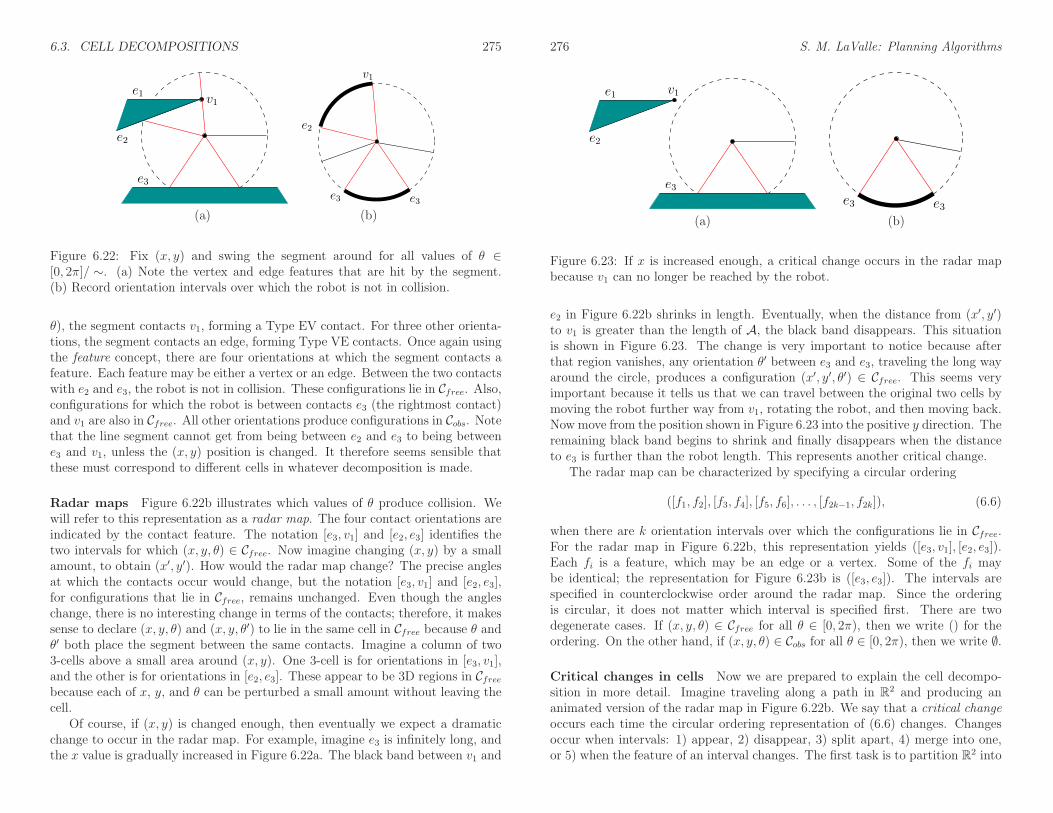
Figure 6.22: Fix (x, y) and swing the segment around for all values of θ ∈[0, 2π]/ ∼. (a) Note the vertex and edge features that are hit by the segment.(b) Record orientation intervals over which the robot is not in collision.
θ), the segment contacts v1, forming a Type EV contact. For three other orienta-tions, the segment contacts an edge, forming Type VE contacts. Once again usingthe feature concept, there are four orientations at which the segment contacts afeature. Each feature may be either a vertex or an edge. Between the two contactswith e2 and e3, the robot is not in collision. These configurations lie in Cfree. Also,configurations for which the robot is between contacts e3 (the rightmost contact)and v1 are also in Cfree. All other orientations produce configurations in Cobs. Notethat the line segment cannot get from being between e2 and e3 to being betweene3 and v1, unless the (x, y) position is changed. It therefore seems sensible thatthese must correspond to different cells in whatever decomposition is made.
Radar maps Figure 6.22b illustrates which values of θ produce collision. Wewill refer to this representation as a radar map. The four contact orientations areindicated by the contact feature. The notation [e3, v1] and [e2, e3] identifies thetwo intervals for which (x, y, θ) ∈ Cfree. Now imagine changing (x, y) by a smallamount, to obtain (x′, y′). How would the radar map change? The precise anglesat which the contacts occur would change, but the notation [e3, v1] and [e2, e3],for configurations that lie in Cfree, remains unchanged. Even though the angleschange, there is no interesting change in terms of the contacts; therefore, it makessense to declare (x, y, θ) and (x, y, θ′) to lie in the same cell in Cfree because θ andθ′ both place the segment between the same contacts. Imagine a column of two3-cells above a small area around (x, y). One 3-cell is for orientations in [e3, v1],and the other is for orientations in [e2, e3]. These appear to be 3D regions in Cfreebecause each of x, y, and θ can be perturbed a small amount without leaving thecell.
Of course, if (x, y) is changed enough, then eventually we expect a dramaticchange to occur in the radar map. For example, imagine e3 is infinitely long, andthe x value is gradually increased in Figure 6.22a. The black band between v1 and
276 S. M. LaValle: Planning Algorithms
e2
e1
e3
v1
e3e3
(a) (b)
Figure 6.23: If x is increased enough, a critical change occurs in the radar mapbecause v1 can no longer be reached by the robot.
e2 in Figure 6.22b shrinks in length. Eventually, when the distance from (x′, y′)to v1 is greater than the length of A, the black band disappears. This situationis shown in Figure 6.23. The change is very important to notice because afterthat region vanishes, any orientation θ′ between e3 and e3, traveling the long wayaround the circle, produces a configuration (x′, y′, θ′) ∈ Cfree. This seems veryimportant because it tells us that we can travel between the original two cells bymoving the robot further way from v1, rotating the robot, and then moving back.Now move from the position shown in Figure 6.23 into the positive y direction. Theremaining black band begins to shrink and finally disappears when the distanceto e3 is further than the robot length. This represents another critical change.
The radar map can be characterized by specifying a circular ordering
([f1, f2], [f3, f4], [f5, f6], . . . , [f2k−1, f2k]), (6.6)
when there are k orientation intervals over which the configurations lie in Cfree.For the radar map in Figure 6.22b, this representation yields ([e3, v1], [e2, e3]).Each fi is a feature, which may be an edge or a vertex. Some of the fi maybe identical; the representation for Figure 6.23b is ([e3, e3]). The intervals arespecified in counterclockwise order around the radar map. Since the orderingis circular, it does not matter which interval is specified first. There are twodegenerate cases. If (x, y, θ) ∈ Cfree for all θ ∈ [0, 2π), then we write () for theordering. On the other hand, if (x, y, θ) ∈ Cobs for all θ ∈ [0, 2π), then we write ∅.
Critical changes in cells Now we are prepared to explain the cell decompo-sition in more detail. Imagine traveling along a path in R2 and producing ananimated version of the radar map in Figure 6.22b. We say that a critical changeoccurs each time the circular ordering representation of (6.6) changes. Changesoccur when intervals: 1) appear, 2) disappear, 3) split apart, 4) merge into one,or 5) when the feature of an interval changes. The first task is to partition R2 into

6.3. CELL DECOMPOSITIONS 277
e
L
v
L
(a) (b)
ev
L
Lv1
v2
(c) (d)
Figure 6.24: Four of the five cases that produce critical curves in R2.
maximal 2-cells over which no critical changes occur. Each one of these 2-cells,R, represents the projection of a strip of 3-cells in Cfree. Each 3-cell is defined asfollows. Let R, [fi, fi+1] denote the 3D region in Cfree for which (x, y) ∈ R andθ places the segment between contacts fi and fi+1. The cylinder of cells above Ris given by R, [fi, fi+1] for each interval in the circular ordering representation,(6.6). If any orientation is possible because A never contacts an obstacle while inR, then we write R.
What are the positions in R2 that cause critical changes to occur? It turnsout that there are five different cases to consider, each of which produces a set ofcritical curves in R2. When one of these curves is crossed, a critical change occurs.If none of these curves is crossed, then no critical change can occur. Therefore,these curves precisely define the boundaries of the desired 2-cells in R2. Let Ldenote the length of the robot (which is the line segment).
Consider how the five cases mentioned above may occur. Two of the five caseshave already been observed in Figures 6.22 and 6.23. These appear in Figures6.24a and Figures 6.24b, and occur if (x, y) is within L of an edge or a vertex.The third and fourth cases are shown in Figures 6.24c and 6.24d, respectively. Thethird case occurs because crossing the curve causes A to change between beingable to touch e and being able to touch v. This must be extended from any edgeat an endpoint that is a reflex vertex (interior angle is greater than π). The fourthcase is actually a return of the bitangent case from Figure 6.10, which arose for
278 S. M. LaValle: Planning Algorithms
v
eA
L
Figure 6.25: The fifth case is the most complicated. It results in a fourth-degreealgebraic curve called the Conchoid of Nicomedes.
R1 R2 R3 R4
R6R7
R9
R10
R11
R12
R13
A
R8
R5
e3
e2
x2
x1
e4
e1
Figure 6.26: The critical curves form the boundaries of the noncritical regions inR2.
the shortest path graph. If the vertices are within L of each other, then a linearcritical curve is generated because A is no longer able to touch v2 when crossing itfrom right to left. Bitangents always produce curves in pairs; the curve above v2is not shown. The final case, shown in Figure 6.25, is the most complicated. It is afourth-degree algebraic curve called the Conchoid of Nicomedes, which arises fromA being in simultaneous contact between v and e. Inside of the teardrop-shapedcurve, A can contact e but not v. Just outside of the curve, it can touch v. If thexy coordinate frame is placed so that v is at (0, 0), then the equation of the curveis
(x2 − y2)(y + d)2 − y2L2 = 0, (6.7)
in which d is the distance from v to e.Putting all of the curves together generates a cell decomposition of R2. There
are noncritical regions, over which there is no change in (6.6); these form the2-cells. The boundaries between adjacent 2-cells are sections of the critical curvesand form 1-cells. There are also 0-cells at places where critical curves intersect.

6.3. CELL DECOMPOSITIONS 279
xy planeR R′
θ
Figure 6.27: Connections are made between neighboring 3-cells that lie aboveneighboring noncritical regions.
Figure 6.26 shows an example adapted from [47]. Note that critical curves are notdrawn if their corresponding configurations are all in Cobs. The method still workscorrectly if they are included, but unnecessary cell boundaries are made. Just forfun, they could be used to form a nice cell decomposition of Cobs, in addition toCfree. Since Cobs is avoided, is seems best to avoid wasting time on decomposingit. These unnecessary cases can be detected by imagining that A is a laser withrange L. As the laser sweeps around, only features that are contacted by the laserare relevant. Any features that are hidden from view of the laser correspond tounnecessary boundaries.
After the cell decomposition has been constructed in R2, it needs to be liftedinto R2× [0, 2π]/ ∼. This generates a cylinder of 3-cells above each 2D noncriticalregion, R. The roadmap could easily be defined to have a vertex for every 3-celland 2-cell, which would be consistent with previous cell decompositions; however,vertices at 2-cells are not generated here to make the coming example easier tounderstand. Each 3-cell, R, [fi, fi+1], corresponds to the vertex in a roadmap.The roadmap edges connect neighboring 3-cells that have a 2-cell as part of theircommon boundary. This means that in R2 they share a one-dimensional portionof a critical curve.
Constructing the roadmap The problem is to determine which 3-cells areactually adjacent. Figure 6.27 depicts the cases in which connections need to bemade. The xy plane is represented as one axis (imagine looking in a directionparallel to it). Consider two neighboring 2-cells (noncritical regions), R and R′,in the plane. It is assumed that a 1-cell (critical curve) in R2 separates them. Thetask is to connect together 3-cells in the cylinders above R and R′. If neighbor-ing cells share the same feature pair, then they are connected. This means thatR, [fi, fi+1] and R′, [fi, fi+1] must be connected. In some cases, one feature
280 S. M. LaValle: Planning Algorithms
R7
R5
e3
e2
x2
x1
e4
e1
R10
R9
R8
R13
R11
R12
R2 R3R1 R6R4
Figure 6.28: A depiction of the 3-cells above the noncritical regions. Samplerod orientations are shown for each cell (however, the rod length is shortened forclarity). Edges between cells are shown in Figure 6.29.
may change, while the interval of orientations remains unchanged. This may hap-pen, for example, when the robot changes from contacting an edge to contactinga vertex of the edge. In these cases, a connection must also be made. One caseillustrated in Figure 6.27 is when a splitting or merging of orientation intervalsoccurs. Traveling from R to R′, the figure shows two regions merging into one. Inthis case, connections must be made from each of the original two 3-cells to themerged 3-cell. When constructing the roadmap edges, sample points of both the3-cells and 2-cells should be used to ensure collision-free paths are obtained, asin the case of the vertical decomposition in Section 6.2.2. Figure 6.28 depicts thecells for the example in Figure 6.26. Each noncritical region has between one andthree cells above it. Each of the various cells is indicated by a shortened robot thatpoints in the general direction of the cell. The connections between the cells arealso shown. Using the noncritical region and feature names from Figure 6.26, theresulting roadmap is depicted abstractly in Figure 6.29. Each vertex represents a3-cell in Cfree, and each edge represents the crossing of a 2-cell between adjacent3-cells. To make the roadmap consistent with previous roadmaps, we could inserta vertex into every edge and force the path to travel through the sample point ofthe corresponding 2-cell.
Once the roadmap has been constructed, it can be used in the same way asother roadmaps in this chapter to solve a query. Many implementation details havebeen neglected here. Due to the fifth case, some of the region boundaries in R2 arefourth-degree algebraic curves. Ways to prevent the explicit characterization ofevery noncritical region boundary, and other implementation details, are coveredin [7]. Some of these details are also summarized in [47].

6.4. COMPUTATIONAL ALGEBRAIC GEOMETRY 281
R1, [e1, e3] R2, [e1, e3] R3, [e1, e3] R4, [e1, e3] R9, [e1, e3] R10, [v1, e3]
R5, [e1, e3]
R8, [v1, e3]R6, [e1, e3]
R7, [e4, e3]R6, [e4, e2]R5, [e4, v1]
R8, [e4, e2]
R4, [e4, v1] R9, [e4, e2] R10, [e4, e2] R11, [e4, e2] R12, [e4, e2] R13, [e4, e2]
R1, [e3, e1] R2, [e3, v1] R3, [e3, e4]
R9, [e3, e4]
R10, [e3, e4]R11, [e3, e4]R12, [v1, e4]R13, [e2, e4]
R4, [e3, e4]
Figure 6.29: The roadmap corresponding to the example in Figure 6.26.
Complexity How many cells can there possibly be in the worst case? Firstcount the number of noncritical regions in R2. There are O(n) different ways togenerate critical curves of the first three types because each corresponds to a singlefeature. Unfortunately, there are O(n2) different ways to generate bitangents andthe Conchoid of Nicomedes because these are based on pairs of features. Assumingno self-intersections, a collection of O(n2) curves in R2, may intersect to generateat most O(n4) regions. Above each noncritical region in R2, there could be acylinder of O(n) 3-cells. Therefore, the size of the cell decomposition is O(n5)in the worst case. In practice, however, it is highly unlikely that all of theseintersections will occur, and the number of cells is expected to be reasonable.In [67], an O(n5)-time algorithm is given to construct the cell decomposition.Algorithms that have much better running time are mentioned in Section 6.5.3,but they are more complicated to understand and implement.
6.4 Computational Algebraic Geometry
This section presents algorithms that are so general that they solve any prob-lem of Formulation 4.1 and even the closed-chain problems of Section 4.4. Itis amazing that such algorithms exist; however, it is also unfortunate that theyare both extremely challenging to implement and not efficient enough for mostapplications. The concepts and tools of this section were mostly developed inthe context of computational real algebraic geometry [9, 25]. They are powerful
282 S. M. LaValle: Planning Algorithms
enough to conquer numerous problems in robotics, computer vision, geometricmodeling, computer-aided design, and geometric theorem proving. One of theseproblems happens to be motion planning, for which the connection to computa-tional algebraic geometry was first recognized in [68].
6.4.1 Basic Definitions and Concepts
This section builds on the semi-algebraic model definitions from Section 3.1 andthe polynomial definitions from Section 4.4.1. It will be assumed that C ⊆ Rn,which could for example arise by representing each copy of SO(2) or SO(3) in its2× 2 or 3× 3 matrix form. For example, in the case of a 3D rigid body, we knowthat C = R3 ×RP3, which is a six-dimensional manifold, but it can be embeddedin R12, which is obtained from the Cartesian product of R3 and the set of all3× 3 matrices. The constraints that force the matrices to lie in SO(2) or SO(3)are polynomials, and they can therefore be added to the semi-algebraic models ofCobs and Cfree. If the dimension of C is less than n, then the algorithm presentedbelow is sufficient, but there are some representation and complexity issues thatmotivate using a special parameterization of C to make both dimensions the samewhile altering the topology of C to become homeomorphic to Rn. This is discussedbriefly in Section 6.4.2.
Suppose that the models in Rn are all expressed using polynomials fromQ[x1, . . . , xn], the set of polynomials6 over the field of rational numbers Q. Letf ∈ Q[x1, . . . , xn] denote a polynomial.
Tarski sentences Recall the logical predicates that were formed in Section 3.1.They will be used again here, but now they are defined with a little more flexibility.For any f ∈ Q[x1, . . . , xn], an atom is an expression of the form f ⊲⊳ 0, in which ⊲⊳may be any relation in the set =, 6=, <,>,≤,≥. In Section 3.1, such expressionswere used to define logical predicates. Here, we assume that relations other than≤ can be used and that the vector of polynomial variables lies in Rn.
A quantifier-free formula, φ(x1, . . . , xn), is a logical predicate composed ofatoms and logical connectives, “and,” “or,” and “not,” which are denoted by ∧,∨, and ¬, respectively. Each atom itself is considered as a logical predicate thatyields true if and only if the relation is satisfied when the polynomial is evaluatedat the point (x1, . . . , xn) ∈ Rn.
Example 6.2 (An Example Predicate) Let φ be a predicate over R3, definedas
φ(x1, x2, x3) = (x21x3 − x42 < 0)∨(
¬(3x2x3 6= 0)∧ (2x23 − x1x2x3 + 2 ≥ 0))
. (6.8)
The precedence order of the connectives follows the laws of Boolean algebra.
6It will be explained shortly why Q[x1, . . . , xn] is preferred over R[x1, . . . , xn].

6.4. COMPUTATIONAL ALGEBRAIC GEOMETRY 283
Let a quantifier Q be either of the symbols, ∀, which means “for all,” or ∃,which means “there exists.” A Tarski sentence Φ is a logical predicate that mayadditionally involve quantifiers on some or all of the variables. In general, a Tarskisentence takes the form
Φ(x1, . . . , xn−k) = (Qz1)(Qz2) . . . (Qzk) φ(z1, . . . , zk, x1, . . . , xn−k), (6.9)
in which the zi are the quantified variables, the xi are the free variables, and φ isa quantifier-free formula. The quantifiers do not necessarily have to appear at theleft to be a valid Tarski sentence; however, any expression can be manipulatedinto an equivalent expression that has all quantifiers in front, as shown in (6.9).The procedure for moving quantifiers to the front is as follows [55]: 1) Eliminateany redundant quantifiers; 2) rename some of the variables to ensure that thesame variable does not appear both free and bound; 3) move negation symbols asfar inward as possible; and 4) push the quantifiers to the left.
Example 6.3 (Several Tarski Sentences) Tarski sentences that have no freevariables are either true or false in general because there are no arguments onwhich the results depend. The sentence
Φ = ∀x∃y (x2 − y < 0), (6.10)
is true because for any x ∈ R, some y ∈ R can always be chosen so that y > x2.In the general notation of (6.9), this example becomes Qz1 = ∀x, Qz2 = ∃y, andφ(z1, z2) = (x2 − y < 0).
Swapping the order of the quantifiers yields the Tarski sentence
Φ = ∃y∀x (x2 − y < 0), (6.11)
which is false because for any y, there is always an x such that x2 > y.Now consider a Tarski sentence that has a free variable:
Φ(z) = ∃y∀x (x2 − zx2 − y < 0). (6.12)
This yields a function Φ : R → true, false, in which
Φ(z) =
true if z ≥ 1false if z < 1.
(6.13)
An equivalent quantifier-free formula φ can be defined as φ(z) = (z > 1), whichtakes on the same truth values as the Tarski sentence in (6.12). This might makeyou wonder whether it is always possible to make a simplification that eliminatesthe quantifiers. This is called the quantifier-elimination problem, which will beexplained shortly.
284 S. M. LaValle: Planning Algorithms
The decision problem The sentences in (6.10) and (6.11) lead to an interestingproblem. Consider the set of all Tarski sentences that have no free variables. Thesubset of these that are true comprise the first-order theory of the reals. Canan algorithm be developed to determine whether such a sentence is true? Thisis called the decision problem for the first-order theory of the reals. At firstit may appear hopeless because Rn is uncountably infinite, and an algorithmmust work with a finite set. This is a familiar issue faced throughout motionplanning. The sampling-based approaches in Chapter 5 provided one kind ofsolution. This idea could be applied to the decision problem, but the resultinglack of completeness would be similar. It is not possible to check all possible pointsin Rn by sampling. Instead, the decision problem can be solved by constructinga combinatorial representation that exactly represents the decision problem bypartitioning Rn into a finite collection of regions. Inside of each region, only onepoint needs to be checked. This should already seem related to cell decompositionsin motion planning; it turns out that methods developed to solve the decisionproblem can also conquer motion planning.
The quantifier-elimination problem Another important problem was exem-plified in (6.12). Consider the set of all Tarski sentences of the form (6.9), whichmay or may not have free variables. Can an algorithm be developed that takesa Tarski sentence Φ and produces an equivalent quantifier-free formula φ? Letx1, . . . , xn denote the free variables. To be equivalent, both must take on thesame true values over Rn, which is the set of all assignments (x1, . . . , xn) for thefree variables.
Given a Tarski sentence, (6.9), the quantifier-elimination problem is to find aquantifier-free formula φ such that
Φ(x1, . . . , xn) = φ(x1, . . . , xn) (6.14)
for all (x1, . . . , xn) ∈ Rn. This is equivalent to constructing a semi-algebraic modelbecause φ can always be expressed in the form
φ(x1, . . . , xn) =k∨
i=1
mi∧
j=1
(fi,j(x1, . . . , xn) ⊲⊳ 0) , (6.15)
in which ⊲⊳ may be either <, =, or >. This appears to be the same (3.6), exceptthat (6.15) uses the relations <, =, and > to allow open and closed semi-algebraicsets, whereas (3.6) only used ≤ to construct closed semi-algebraic sets for O andA.
Once again, the problem is defined on Rn, which is uncountably infinite, butan algorithm must work with a finite representation. This will be achieved by thecell decomposition technique presented in Section 6.4.2.

6.4. COMPUTATIONAL ALGEBRAIC GEOMETRY 285
(−1,−1, 1, 1) (−1, 1,−1, 1)
(−1, 1, 1, 0)
(−1, 1, 0, 1)(−1, 0, 1, 1)
(1, 1, 1, 1)
(0, 1, 1, 1)(−1, 1, 1,−1)
(−1, 1, 1, 1)
Figure 6.30: A semi-algebraic decomposition of the gingerbread face yields 9 sign-invariant regions.
Semi-algebraic decomposition As stated in Section 6.3.1, motion planninginside of each cell in a complex should be trivial. To solve the decision andquantifier-elimination problems, a cell decomposition was developed for whichthese problems become trivial in each cell. The decomposition is designed so thatonly a single point in each cell needs to be checked to solve the decision problem.
The semi-algebraic set Y ⊆ Rn that is expressed with (6.15) is
Y =k⋃
i=1
mi⋂
j=1
(x1, . . . , xn) ∈ Rn | sgn(fi,j(x1, . . . , xn)) = si,j , (6.16)
in which sgn is the sign function, and each si,j ∈ −1, 0, 1, which is the rangeof sgn. Once again the nice relationship between set-theory and logic, which wasdescribed in Section 3.1, appears here. We convert from a set-theoretic descriptionto a logical predicate by changing ∪ and ∩ to ∨ and ∧, respectively.
Let F denote the set ofm =∑k
i=1mi polynomials that appear in (6.16). A signassignment with respect to F is a vector-valued function, sgnF : Rn → −1, 0, 1m.Each f ∈ F has a corresponding position in the sign assignment vector. Atthis position, the sign, sgn(f(x1, . . . , xn)) ∈ −1, 0, 1, appears. A semi-algebraicdecomposition is a partition of Rn into a finite set of connected regions that are eachsign invariant. This means that inside of each region, sgnF must remain constant.The regions will not be called cells because a semi-algebraic decomposition is notnecessarily a singular complex as defined in Section 6.3.1; the regions here maycontain holes.
Example 6.4 (Sign assignment) Recall Example 3.1 and Figure 3.4 from Sec-tion 3.1.2. Figure 3.4a shows a sign assignment for a case in which there is only
286 S. M. LaValle: Planning Algorithms
one polynomial, F = x2 + y2 − 4. The sign assignment is defined as
sgnF(x, y) =
−1 if x2 + y2 − 4 < 00 if x2 + y2 − 4 = 01 if x2 + y2 − 4 > 0.
(6.17)
Now consider the sign assignment sgnF , shown in Figure 6.30 for the gin-gerbread face of Figure 3.4b. The polynomials of the semi-algebraic model areF = f1, f2, f3, f4, as defined in Example 3.1. In order, these are the “head,” “lefteye,” “right eye,” and “mouth.” The sign assignment produces a four-dimensionalvector of signs. Note that if (x, y) lies on one of the zeros of a polynomial in F ,then a 0 appears in the sign assignment. If the curves of two or more of thepolynomials had intersected, then the sign assignment would produce more thanone 0 at the intersection points.
For the semi-algebraic decomposition for the gingerbread face in Figure 6.30,there are nine regions. Five 2D regions correspond to: 1) being outside of theface, 2)inside of the left eye, 3) inside of the right eye, 4) inside of the mouth,and 5) inside of the face but outside of the mouth and eyes. There are four 1Dregions, each of which corresponds to points that lie on one of the zero sets of apolynomial. The resulting decomposition is not a singular complex because the(−1, 1, 1, 1) region contains three holes.
A decomposition such as the one in Figure 6.30 would not be very usefulfor motion planning because of the holes in the regions. Further refinement isneeded for motion planning, which is fortunately produced by cylindrical algebraicdecomposition. On the other hand, any semi-algebraic decomposition is quiteuseful for solving the decision problem. Only one point needs to be checked insideof each region to determine whether some Tarski sentence that has no free variablesis true. Why? If the polynomial signs cannot change over some region, thenthe true/false value of the corresponding logical predicate, Φ, cannot change.Therefore, it sufficient only to check one point per sign-invariant region.
6.4.2 Cylindrical Algebraic Decomposition
Cylindrical algebraic decomposition is a general method that produces a cylin-drical decomposition in the same sense considered in Section 6.3.2 for polygonsin R2 and also the decomposition in Section 6.3.4 for the line-segment robot. Itis also referred to as Collins decomposition after its original developer [4, 22, 23].The decomposition in Figure 6.19 can even be considered as a cylindrical alge-braic decomposition for a semi-algebraic set in which every geometric primitive isa linear polynomial. In this section, such a decomposition is generalized to anysemi-algebraic set in Rn.
The idea is to develop a sequence of projections that drops the dimensionof the semi-algebraic set by one each time. Initially, the set is defined over Rn,

6.4. COMPUTATIONAL ALGEBRAIC GEOMETRY 287
and after one projection, a semi-algebraic set is obtained in Rn−1. Eventually,the projection reaches R, and a univariate polynomial is obtained for which thezeros are at the critical places where cell boundaries need to be formed. A celldecomposition of 1-cells (intervals) and 0-cells is formed by partitioning R. Thesequence is then reversed, and decompositions are formed from R2 up to Rn. Eachiteration starts with a cell decomposition in Ri and lifts it to obtain a cylinder ofcells in Ri+1. Figure 6.35 shows how the decomposition looks for the gingerbreadexample; since n = 2, it only involves one projection and one lifting.
Semi-algebraic projections are semi-algebraic The following is implied bythe Tarski-Seidenberg Theorem [9]:
A projection of a semi-algebraic set from dimension n to dimensionn− 1 is a semi-algebraic set.
This gives a kind of closure of semi-algebraic sets under projection, which is re-quired to ensure that every projection of a semi-algebraic set in Ri leads to asemi-algebraic set in Ri−1. This property is actually not true for (real) algebraicvarieties, which were introduced in Section 4.4.1. Varieties are defined using onlythe = relation and are not closed under the projection operation. Therefore, it isa good thing (not just a coincidence!) that we are using semi-algebraic sets.
Real algebraic numbers As stated previously, the sequence of projections endswith a univariate polynomial over R. The sides of the cells will be defined basedon the precise location of the roots of this polynomial. Furthermore, representinga sample point for a cell of dimension k in a complex in Rn for k < n requiresperfect precision. If the coordinates are slightly off, the point will lie in a differentcell. This raises the complicated issue of how these roots are represented andmanipulated in a computer.
For univariate polynomials of degree 4 or less, formulas exist to compute allof the roots in terms of functions of square roots and higher order roots. FromGalois theory [39, 62], it is known that such formulas and nice expressions forroots do not exist for most higher degree polynomials, which can certainly arisein the complicated semi-algebraic models that are derived in motion planning.The roots in R could be any real number, and many real numbers require infiniterepresentations.
One way of avoiding this mess is to assume that only polynomials inQ[x1, . . . , xn]are used, instead of the more general R[x1, . . . , xn]. The field Q is not alge-braically closed because zeros of the polynomials lie outside of Qn. For example, iff(x1) = x21 − 2, then f = 0 for x1 = ±
√2, and
√2 6∈ Q. However, some elements
of R can never be roots of a polynomial in Q[x1, . . . , xn].The set A of all real roots to all polynomials in Q[x] is called the set of real
algebraic numbers. The set A ⊂ R actually represents a field (recall from Section4.4.1). Several nice algorithmic properties of the numbers in A are 1) they all have
288 S. M. LaValle: Planning Algorithms
finite representations, 2) addition and multiplication operations on elements of Acan be computed in polynomial time, and 3) conversions between different repre-sentations of real algebraic numbers can be performed in polynomial time. Thismeans that all operations can be computed efficiently without resorting to somekind of numerical approximation. In some applications, such approximations arefine; however, for algebraic decompositions, they destroy critical information bypotentially confusing roots (e.g., how can we know for sure whether a polynomialhas a double root or just two roots that are very close together?).
The details are not presented here, but there are several methods for rep-resenting real algebraic numbers and the corresponding algorithms for manipu-lating them efficiently. The running time of cylindrical algebraic decompositionultimately depends on this representation. In practice, a numerical root-findingmethod that has a precision parameter, ǫ, can be used by choosing ǫ small enoughto ensure that roots will not be confused. A sufficiently small value can be de-termined by applying gap theorems, which give lower bounds on the amount ofreal root separation, expressed in terms of the polynomial coefficients [16]. Somemethods avoid requiring a precision parameter. One well-known example is thederivation of a Sturm sequence of polynomials based on the given polynomial.The polynomials in the Sturm sequence are then used to find isolating intervalsfor each of the roots [9]. The polynomial, together with its isolating interval, canbe considered as an exact root representation. Algebraic operations can even beperformed using this representation in time O(d lg2 d), in which d is the degreeof the polynomial [68]. See [9, 16, 68] for detailed presentations on the exactrepresentation and calculation with real algebraic numbers.
One-dimensional decomposition To explain the cylindrical algebraic decom-position method, we first perform a semi-algebraic decomposition of R, which isthe final step in the projection sequence. Once this is explained, then the multi-dimensional case follows more easily.
Let F be a set of m univariate polynomials,
F = fi ∈ Q[x] | i = 1, . . . ,m, (6.18)
which are used to define some semi-algebraic set in R. The polynomials in F couldcome directly from a quantifier-free formula φ (which could even appear inside ofa Tarski sentence, as in (6.9)).
Define a single polynomial as f =∏m
i=1 fi. Suppose that f has k distinct, realroots, which are sorted in increasing order:
−∞ < β1 < β2 < · · · < βi−1 < βi < βi+1 < · · · < βk < ∞. (6.19)
The one-dimensional semi-algebraic decomposition is given by the followingsequence of alternating 1-cells and 0-cells:
(−∞, β1), [β1, β1], (β1, β2), . . . , (βi−1, βi), [βi, βi],
(βi, βi+1), . . . , [βk, βk], (βk,∞).(6.20)

6.4. COMPUTATIONAL ALGEBRAIC GEOMETRY 289
f1(x) = x2 − 2x f2(x) = x2 − 4x + 3
2 310R
−1
Figure 6.31: Two parabolas are used to define the semi-algebraic set [1, 2].
R0
[3, 3](2, 3)(1, 2)[1, 1] [2, 2](0, 1)[0, 0](−∞, 0) (3,∞)
2 31
Figure 6.32: A semi-algebraic decomposition for the polynomials in Figure 6.31.
Any semi-algebraic set that can be expressed using the polynomials in F canalso be expressed as the union of some of the 0-cells and 1-cells given in (6.20).This can also be considered as a singular complex (it can even be considered as asimplicial complex, but this does not extend to higher dimensions).
Sample points can be generated for each of the cells as follows. For the un-bounded cells [−∞, β1) and (βk,∞], valid samples are β1 − 1 and βk + 1, respec-tively. For each finite 1-cell, (βi, βi+1), the midpoint (βi + βi+1)/2 produces asample point. For each 0-cell, [βi, βi], the only choice is to use βi as the samplepoint.
Example 6.5 (One-Dimensional Decomposition) Figure 6.31 shows a semi-algebraic subset of R that is defined by two polynomials, f1(x) = x2 − 2x andf2(x) = x2 − 4x+ 3. Here, F = f1, f2. Consider the quantifier-free formula
φ(x) = (x2 − 2x ≥ 0) ∧ (x2 − 4x+ 3 ≥ 0). (6.21)
The semi-algebraic decomposition into five 1-cells and four 0-cells is shown inFigure 6.32. Each cell is sign invariant. The sample points for the 1-cells are −1,1/2, 3/2, 5/2, and 4, respectively. The sample points for the 0-cells are 0, 1, 2,and 3, respectively.
A decision problem can be nicely solved using the decomposition. Supposea Tarski sentence that uses the polynomials in F has been given. Here is onepossibility:
Φ = ∃x[(x2 − 2x ≥ 0) ∧ (x2 − 4x+ 3 ≥ 0)] (6.22)
The sample points alone are sufficient to determine whether Φ is true or false.Once x = 1 is attempted, it is discovered that Φ is true. The quantifier-elimination problem cannot yet be considered because more dimensions are needed.
290 S. M. LaValle: Planning Algorithms
Folding over Intersection
Figure 6.33: Critical points occur either when the surface folds over in the verticaldirection or when surfaces intersect.
The inductive step to higher dimensions Now consider constructing a cylin-drical algebraic decomposition for Rn (note the decomposition is actually semi-algebraic). Figure 6.35 shows an example for R2. First consider how to iterativelyproject the polynomials down to R to ensure that when the decomposition of Rn
is constructed, the sign-invariant property is maintained. The resulting decompo-sition corresponds to a singular complex.
There are two cases that cause cell boundaries to be formed, as shown in Figure6.33. Let Fn denote the original set of polynomials inQ[x1, . . . , xn] that are used todefine the semi-algebraic set (or Tarski sentence) in Rn. Form a single polynomialf =
∏m
i=1 fi. Let f ′ = ∂f/∂xn, which is also a polynomial. Let g = GCD(f, f ′),which is the greatest common divisor of f and f ′. The set of zeros of g is the set ofall points that are zeros of both f and f ′. Being a zero of f ′ means that the surfacegiven by f = 0 does not vary locally when perturbing xn. These are places wherea cell boundary needs to be formed because the surface may fold over itself inthe xn direction, which is not permitted for a cylindrical decomposition. Anotherplace where a cell boundary needs to be formed is at the intersection of two ormore polynomials in Fn. The projection technique from Rn to Rn−1 generatesa set, Fn−1, of polynomials in Q[x1, . . . , xn−1] that satisfies these requirements.The polynomials Fn−1 have the property that at least one contains a zero pointbelow every point in x ∈ Rn for which f(x) = 0 and f ′(x) = 0, or polynomialsin Fn intersect. The projection method that constructs Fn−1 involves computingprinciple subresultant coefficients, which are covered in [9, 69]. Resultants, ofwhich the subresultants are an extension, are covered in [25].
The polynomials in Fn−1 are then projected to Rn−2 to obtain Fn−2. Thisprocess continues until F1 is obtained, which is a set of polynomials in Q[x1]. Aone-dimensional decomposition is formed, as defined earlier. From F1, a singlepolynomial is formed by taking the product, and R is partitioned into 0-cells and1-cells. We next describe the process of lifting a decomposition over Ri−1 up toRi. This technique is applied iteratively until Rn is reached.

6.4. COMPUTATIONAL ALGEBRAIC GEOMETRY 291
Assume inductively that a cylindrical algebraic decomposition has been com-puted for a set of polynomials Fi−1 in Q[x1, . . . , xi−1]. The decomposition consistsof k-cells for which 0 ≤ k ≤ i. Let p = (x1, . . . , xi−1) ∈ Ri−1. For each one of thek-cells Ci−1, a cylinder over Ci−1 is defined as the (k + 1)-dimensional set
(p, xi) ∈ Ri | p ∈ Ci−1. (6.23)
The cylinder is sliced into a strip of k-dimensional and k+ 1-dimensional cells byusing polynomials in Fi. Let fj denote one of the ℓ slicing polynomials in thecylinder, sorted in increasing xi order as f1, f2, . . ., fj, fj+1, . . ., fℓ. The followingkinds of cells are produced (see Figure 6.34):
1. Lower unbounded sector:
(p, xi) ∈ Ri | p ∈ Ci−1 and xi < f1(p) . (6.24)
2. Section:(p, xi) ∈ Ri | p ∈ Ci−1 and xi = fj(p) . (6.25)
3. Bounded sector:
(p, xi) ∈ Ri | p ∈ Ci−1 and fj(p) < xi < fj+1(p) . (6.26)
4. Upper unbounded sector:
(p, xi) ∈ Ri | p ∈ Ci−1 and fℓ(p) < xi . (6.27)
There is one degenerate possibility in which there are no slicing polynomials andthe cylinder over Ci−1 can be extended into one unbounded cell. In general, thesample points are computed by picking a point in p ∈ Ci−1 and making a verticalcolumn of samples of the form (p, xi). A polynomial in Q[xi] can be generated,and the samples are placed using the same assignment technique that was usedfor the one-dimensional decomposition.
Example 6.6 (Mutilating the Gingerbread Face) Figure 6.35 shows a cylin-drical algebraic decomposition of the gingerbread face. Observe that the resultingcomplex is very similar to that obtained in Figure 6.19.
Note that the cells do not necessarily project onto a rectangular set, as in thecase of a higher dimensional vertical decomposition. For example, a generic n-cellCn for a decomposition of Rn is described as the open set of (x1, . . . , xn) ∈ Rn
such that
• C0 < xn < C ′
0 for some 0-cells C0, C′
0 ∈ R, which are roots of some f, f ′ ∈ F1.
292 S. M. LaValle: Planning Algorithms
f1
fj
Ci−1
fj+1
fℓ
Figure 6.34: A cylinder over every k-cell Ci−1 is formed. A sequence of poly-nomials, f1, . . ., fℓ, slices the cylinder into k-dimensional sections and (k + 1)-dimensional sectors.
• (xn−1, xn) lies between C1 and C ′
1 for some 1-cells C1, C′
1, which are zerosof some f, f ′ ∈ F2.
...
• (xn−i+1, . . . , xn) lies between Ci−1 and C′
i−1 for some i-cells Ci−1, C′
i−1, whichare zeros of some f, f ′ ∈ Fi.
...
• (x1, . . . , xn) lies between Cn−1 and C ′
n−1 for some (n − 1)-cells Cn−1, C′
n−1,which are zeros of some f, f ′ ∈ Fn.
The resulting decomposition is sign invariant, which allows the decision andquantifier-elimination problems to be solved in finite time. To solve a decisionproblem, the polynomials in Fn are evaluated at every sample point to deter-mine whether one of them satisfies the Tarski sentence. To solve the quantifier-elimination problem, note that any semi-algebraic sets that can be constructedfrom Fn can be defined as a union of some cells in the decomposition. For thegiven Tarski sentence, Fn is formed from all polynomials that are mentioned in

6.4. COMPUTATIONAL ALGEBRAIC GEOMETRY 293
3
5
6
7
9
10
11
12
1 13
14
15
16
17
18
19
20
21
22
23
24
25
26
27
28
29
328
33
342
35
30
364
37
31
R
Figure 6.35: A cylindrical algebraic decomposition of the gingerbread face. Thereare 37 2-cells, 64 1-cells, and 28 0-cells. The straight 1-cells are intervals of thevertical lines, and the curved ones are portions of the zero set of a polynomial inF . The decomposition of R is also shown.
the sentence, and the cell decomposition is performed. Once obtained, the signinformation is used to determine which cells need to be included in the union.The resulting union of cells is designed to include only the points in Rn at whichthe Tarski sentence is true.
Solving a motion planning problem Cylindrical algebraic decompositionis also capable of solving any of the motion planning problems formulated inChapter 4. First assume that C = Rn. As for other decompositions, a roadmap isformed in which every vertex is an n-cell and edges connect every pair of adjacentn-cells by traveling through an (n − 1)-cell. It is straightforward to determineadjacencies inside of a cylinder, but there are several technical details associatedwith determining adjacencies of cells from different cylinders (pages 152–154 of[9] present an example that illustrates the problem). The cells of dimension lessthan n− 1 are not needed for motion planning purposes (just as vertices were notneeded for the vertical decomposition in Section 6.2.2). The query points qI andqG are connected to the roadmap depending on the cell in which they lie, and adiscrete search is performed.
294 S. M. LaValle: Planning Algorithms
If C ⊂ Rn and its dimension is k for k < n, then all of the interesting cells are oflower dimension. This occurs, for example, due to the constraints on the matricesto force them to lie in SO(2) or SO(3). This may also occur for problems fromSection 4.4, in which closed chains reduce the degrees of freedom. The cylindricalalgebraic decomposition method can still solve such problems; however, the exactroot representation problem becomes more complicated when determining the celladjacencies. A discussion of these issues appears in [68]. For the case of SO(2)and SO(3), this complication can be avoided by using stereographic projection tomap S1 or S3 to R or R3, respectively. This mapping removes a single point fromeach, but the connectivity of Cfree remains unharmed. The antipodal identificationproblem for unit quaternions represented by S3 also does not present a problem;there is a redundant copy of C, which does not affect the connectivity.
The running time for cylindrical algebraic decomposition depends on manyfactors, but in general it is polynomial in the number of polynomials in Fn, poly-nomial in the maximum algebraic degree of the polynomials, and doubly expo-nential in the dimension. Complexity issues are covered in more detail in Section6.5.3.
6.4.3 Canny’s Roadmap Algorithm
The doubly exponential running time of cylindrical algebraic decomposition in-spired researchers to do better. It has been shown that quantifier eliminationrequires doubly exponential time [27]; however, motion planning is a differentproblem. Canny introduced a method that produces a roadmap directly from thesemi-algebraic set, rather than constructing a cell decomposition along the way.Since there are doubly exponentially many cells in the cylindrical algebraic de-composition, avoiding this construction pays off. The resulting roadmap methodof Canny solves the motion planning problem in time that is again polynomial inthe number of polynomials and polynomial in the algebraic degree, but it is onlysingly exponential in dimension [14, 16]; see also [9].
Much like the other combinatorial motion planning approaches, it is based onfinding critical curves and critical points. The main idea is to construct linearmappings from Rn to R2 that produce silhouette curves of the semi-algebraicsets. Performing one such mapping on the original semi-algebraic set yields aroadmap, but it might not preserve the original connectivity. Therefore, linearmappings from Rn−1 to R2 are performed on some (n−1)-dimensional slices of theoriginal semi-algebraic set to yield more roadmap curves. This process is appliedrecursively until the slices are already one-dimensional. The resulting roadmapis formed from the union of all of the pieces obtained in the recursive calls. Theresulting roadmap has the same connectivity as the original semi-algebraic set[16].
Suppose that C = Rn. Let F = f1, . . . , fm denote the set of polynomialsthat define the semi-algebraic set, which is assumed to be a disjoint union of

6.4. COMPUTATIONAL ALGEBRAIC GEOMETRY 295
manifolds. Assume that each fi ∈ Q[x1, . . . , xn]. First, a small perturbation tothe input polynomials F is performed to ensure that every sign-invariant set of Rn
is a manifold. This forces the polynomials into a kind of general position, whichcan be achieved with probability one using random perturbations; there are alsodeterministic methods to solve this problem. The general position requirementson the input polynomials and the 2D projection directions are fairly strong, whichhas stimulated more recent work that eliminates many of the problems [9]. Fromthis point onward, it will be assumed that the polynomials are in general position.
Recall the sign-assignment function from Section 6.4.1. Each sign-invariantset is a manifold because of the general position assumption. Canny’s methodcomputes a roadmap for any k-dimensional manifold for k < n. Such a manifoldhas precisely n − k signs that are 0 (which means that points lie precisely onthe zero sets of n − k polynomials in F). At least one of the signs must be 0,which means that Canny’s roadmap actually lies in ∂Cfree (this technically is notpermitted, but the algorithm nevertheless correctly decides whether a solutionpath exists through Cfree).
Recall that each fi is a function, fi : Rn → R. Let x denote (x1, . . . , xn) ∈ Rn.
The k polynomials that have zero signs can be put together sequentially to producea mapping ψ : Rn → Rk. The ith component of the vector ψ(x) is ψi(x) = fi(x).This is closely related to the sign assignment function of Section 6.4.1, except thatnow the real value from each polynomial is directly used, rather than taking itssign.
Now introduce a function g : Rn → Rj, in which either j = 1 or j = 2 (thegeneral concepts presented below work for other values of j, but 1 and 2 are theonly values needed for Canny’s method). The function g serves the same purposeas a projection in cylindrical algebraic decomposition, but note that g immediatelydrops from dimension n to dimension 2 or 1, instead of dropping to n − 1 as inthe case of cylindrical projections.
Let h : Rn → Rk+j denote a mapping constructed directly from ψ and g asfollows. For the ith component, if i ≤ k, then hi(x) = ψi(x) = fi(x). Assumethat k + j ≤ n. If i > k, then hi(x) = gi−k(x). Let Jx(h) denote the Jacobian ofh and be defined at x as
Jx(h) =
∂h1(x)
∂x1· · · ∂h1(x)
∂xn...
...∂hm+k(x)
∂x1· · · ∂hm+k(x)
∂xn
=
∂f1(x)
∂x1· · · ∂f1(x)
∂xn...
...∂fk(x)
∂x1· · · ∂fk(x)
∂xn
∂g1(x)
∂x1· · · ∂g1(x)
∂xn...
...∂gj(x)
∂x1· · · ∂gj(x)
∂xn
. (6.28)
296 S. M. LaValle: Planning Algorithms
A point x ∈ Rn at which Jx(h) is singular is called a critical point. The matrix isdefined to be singular if every (m+k)×(m+k) subdeterminant is zero. Each of thefirst k rows of Jx(h) calculates the surface normal to fi(x) = 0. If these normalsare not linearly independent of the directions given by the last j rows, then thematrix becomes singular. The following example from [13] nicely illustrates thisprinciple.
Example 6.7 (Canny’s Roadmap Algorithm) Let n = 3, k = 1, and j = 1.The zeros of a single polynomial f1 define a 2D subset of R3. Let f1 be the unitsphere, S2, defined as the zeros of the polynomial
f1(x1, x2, x3) = x21 + x22 + x23 − 1. (6.29)
Suppose that g : R3 → R is defined as g(x1, x2, x3) = x1. The Jacobian, (6.28),becomes
(
2x1 2x2 2x31 0 0
)
(6.30)
and is singular when all three of the possible 2 × 2 subdeterminants are zero.This occurs if and only if x2 = x3 = 0. This yields the critical points (−1, 0, 0)and (1, 0, 0) on S2. Note that this is precisely when the surface normals of S2 areparallel to the vector [1 0 0].
Now suppose that j = 2 to obtain g : R3 → R2, and suppose g(x1, x2, x3) =(x1, x2). In this case, (6.28) becomes
2x1 2x2 2x31 0 00 1 0
, (6.31)
which is singular if and only if x3 = 0. The critical points are therefore the x1x2plane intersected with S3, which yields the equator points (all (x1, x2) ∈ R2 suchthat x21 + x22 = 1). In this case, more points are generated because the matrixbecomes degenerate for any surface normal of S2 that is parallel to [1 0 0], [0 1 0]or any linear combination of these.
The first mapping in Example 6.7 yielded two isolated critical points, and thesecond mapping yielded a one-dimensional set of critical points, which is referredto as a silhouette. The union of the silhouette and the isolated critical pointsyields a roadmap for S2. Now consider generalizing this example to obtain thefull algorithm for general n and k. A linear mapping g : Rn → R2 is constructedthat might not be axis-aligned as in Example 6.7 because it must be chosen ingeneral position (otherwise degeneracies might arise in the roadmap). Define ψ tobe the set of polynomials that become zero on the desired manifold on which toconstruct a roadmap. Form the matrix (6.28) and determine the silhouette. Thisis accomplished in general using subresultant techniques that were also needed for
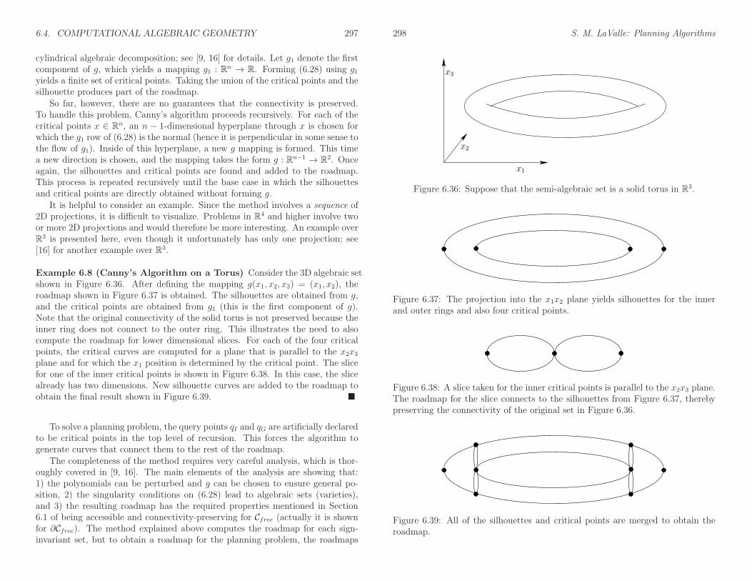
6.4. COMPUTATIONAL ALGEBRAIC GEOMETRY 297
cylindrical algebraic decomposition; see [9, 16] for details. Let g1 denote the firstcomponent of g, which yields a mapping g1 : Rn → R. Forming (6.28) using g1yields a finite set of critical points. Taking the union of the critical points and thesilhouette produces part of the roadmap.
So far, however, there are no guarantees that the connectivity is preserved.To handle this problem, Canny’s algorithm proceeds recursively. For each of thecritical points x ∈ Rn, an n − 1-dimensional hyperplane through x is chosen forwhich the g1 row of (6.28) is the normal (hence it is perpendicular in some sense tothe flow of g1). Inside of this hyperplane, a new g mapping is formed. This timea new direction is chosen, and the mapping takes the form g : Rn−1 → R2. Onceagain, the silhouettes and critical points are found and added to the roadmap.This process is repeated recursively until the base case in which the silhouettesand critical points are directly obtained without forming g.
It is helpful to consider an example. Since the method involves a sequence of2D projections, it is difficult to visualize. Problems in R4 and higher involve twoor more 2D projections and would therefore be more interesting. An example overR3 is presented here, even though it unfortunately has only one projection; see[16] for another example over R3.
Example 6.8 (Canny’s Algorithm on a Torus) Consider the 3D algebraic setshown in Figure 6.36. After defining the mapping g(x1, x2, x3) = (x1, x2), theroadmap shown in Figure 6.37 is obtained. The silhouettes are obtained from g,and the critical points are obtained from g1 (this is the first component of g).Note that the original connectivity of the solid torus is not preserved because theinner ring does not connect to the outer ring. This illustrates the need to alsocompute the roadmap for lower dimensional slices. For each of the four criticalpoints, the critical curves are computed for a plane that is parallel to the x2x3plane and for which the x1 position is determined by the critical point. The slicefor one of the inner critical points is shown in Figure 6.38. In this case, the slicealready has two dimensions. New silhouette curves are added to the roadmap toobtain the final result shown in Figure 6.39.
To solve a planning problem, the query points qI and qG are artificially declaredto be critical points in the top level of recursion. This forces the algorithm togenerate curves that connect them to the rest of the roadmap.
The completeness of the method requires very careful analysis, which is thor-oughly covered in [9, 16]. The main elements of the analysis are showing that:1) the polynomials can be perturbed and g can be chosen to ensure general po-sition, 2) the singularity conditions on (6.28) lead to algebraic sets (varieties),and 3) the resulting roadmap has the required properties mentioned in Section6.1 of being accessible and connectivity-preserving for Cfree (actually it is shownfor ∂Cfree). The method explained above computes the roadmap for each sign-invariant set, but to obtain a roadmap for the planning problem, the roadmaps
298 S. M. LaValle: Planning Algorithms
x1
x3
x2
Figure 6.36: Suppose that the semi-algebraic set is a solid torus in R3.
Figure 6.37: The projection into the x1x2 plane yields silhouettes for the innerand outer rings and also four critical points.
Figure 6.38: A slice taken for the inner critical points is parallel to the x2x3 plane.The roadmap for the slice connects to the silhouettes from Figure 6.37, therebypreserving the connectivity of the original set in Figure 6.36.
Figure 6.39: All of the silhouettes and critical points are merged to obtain theroadmap.

6.5. COMPLEXITY OF MOTION PLANNING 299
from each sign-invariant set must be connected together correctly; fortunately, thishas been solved via the Linking Lemma of [13]. A major problem, however, is thateven after knowing the connectivity of the roadmap, it is a considerable challengeto obtain a parameterization of each curve on the roadmap. For this and manyother technical reasons, no general implementation of Canny’s algorithm appearsto exist at present. Another problem is the requirement of a Whitney stratifica-tion (which can be fixed by perturbation of the input). The Basu-Pollack-Royroadmap algorithm overcomes this problem [9].
6.5 Complexity of Motion Planning
This section summarizes theoretical work that characterizes the complexity ofmotion planning problems. Note that this is not equivalent to characterizing therunning time of particular algorithms. The existence of an algorithm serves asan upper bound on the problem’s difficulty because it is a proof by example thatsolving the problem requires no more time than what is needed by the algorithm.On the other hand, lower bounds are also very useful because they give an indica-tion of the difficulty of the problem itself. Suppose, for example, you are given analgorithm that solves a problem in time O(n2). Does it make sense to try to finda more efficient algorithm? Does it make sense to try to find a general-purposemotion planning algorithm that runs in time that is polynomial in the dimension?Lower bounds provide answers to questions such as this. Usually lower boundsare obtained by concocting bizarre, complicated examples that are allowed by theproblem definition but were usually not considered by the person who first for-mulated the problem. In this line of research, progress is made by either raisingthe lower bound (unless it is already tight) or by showing that a narrower versionof the problem still allows such bizarre examples. The latter case occurs often inmotion planning.
6.5.1 Lower Bounds
Lower bounds have been established for a variety of motion planning problemsand also a wide variety of planning problems in general. To interpret these boundsa basic understanding of the theory of computation is required [38, 73]. This fas-cinating subject will be unjustly summarized in a few paragraphs. A problem is aset of instances that are each carefully encoded as a binary string. An algorithm isformally considered as a Turing machine, which is a finite-state machine that canread and write bits to an unbounded piece of tape. Other models of computationalso exist, such as integer RAM and real RAM (see [11]); there are debates as towhich model is most appropriate, especially when performing geometric compu-tations with real numbers. The standard Turing machine model will be assumedfrom here onward. Algorithms are usually formulated to make a binary output,which involves accepting or rejecting a problem instance that is initially written to
300 S. M. LaValle: Planning Algorithms
P NP PSPACE EXPTIME
Figure 6.40: It is known that P ⊂ EXPTIME is a strict subset; however, it is notknown precisely how large NP and PSPACE are.
the tape and given to the algorithm. In motion planning, this amounts to decidingwhether a solution path exists for a given problem instance.
Languages A language is a set of binary strings associated with a problem. Itrepresents the complete set of instances of a problem. An algorithm is said todecide a language if in finite time it correctly accepts all strings that belong toit and rejects all others. The interesting question is: How much time or space isrequired to decide a language? This question is asked of the problem, under theassumption that the best possible algorithm would be used to decide it. (We caneasily think of inefficient algorithms that waste resources.)
A complexity class is a set of languages that can all be decided within somespecified resource bound. The class P is the set of all languages (and henceproblems) for which a polynomial-time algorithm exists (i.e., the algorithm runsin time O(nk) for some integer k). By definition, an algorithm is called efficientif it decides its associated language in polynomial time.7 If no efficient algorithmexists, then the problem is called intractable. The relationship between severalother classes that often emerge in theoretical motion planning is shown in Figure6.40. The class NP is the set of languages that can be solved in polynomialtime by a nondeterministic Turing machine. Some discussion of nondeterministicmachines appears in Section 11.3.2. Intuitively, it means that solutions can beverified in polynomial time because the machine magically knows which choicesto make while trying to make the decision. The class PSPACE is the set oflanguages that can be decided with no more than a polynomial amount of storagespace during the execution of the algorithm (NPSPACE=PSPACE, so there isno nondeterministic version). The class EXPTIME is the set of languages thatcan be decided in time O(2n
k
) for some integer k. It is known that EXPTIMEis larger than P, but it is not known precisely where the boundaries of NP andPSPACE lie. It might be the case that P = NP = PSPACE (although hardlyanyone believes this), or it could be that NP = PSPACE = EXPTIME.
7Note that this definition may be absurd in practice; an algorithm that runs in time O(n90125)would probably not be too efficient for most purposes.

6.5. COMPLEXITY OF MOTION PLANNING 301
Figure 6.41: Even motion planning for a bunch of translating rectangles inside ofa rectangular box in R2 is PSPACE-hard (and hence, NP-hard).
Hardness and completeness Since an easier class is included as a subset ofa harder one, it is helpful to have a notion of a language (i.e., problem) beingamong the hardest possible within a class. Let X refer to either P, NP, PSPACE,or EXPTIME. A language A is called X-hard if every language B in class X ispolynomial-time reducible to A. In short, this means that in polynomial time,any language in B can be translated into instances for language A, and then thedecisions for A can be correctly translated back in polynomial time to correctlydecide B. Thus, if A can be decided, then within a polynomial-time factor, everylanguage in X can be decided. The hardness concept can even be applied toa language (problem) that does not belong to the class. For example, we candeclare that a language A is NP-hard even if A 6∈NP (it could be harder and lie inEXPTIME, for example). If it is known that the language is both hard for someclass X and is also a member of X, then it is called X-complete (i.e., NP-complete,PSPACE-complete, etc.).8 Note that because of this uncertainty regarding P, NP,and PSPACE, one cannot say that a problem is intractable if it is NP-hard orPSPACE-hard, but one can, however, if the problem is EXPTIME-hard. Oneadditional remark: it is useful to remember that PSPACE-hard implies NP-hard.
Lower bounds for motion planning The general motion planning problem,Formulation 4.1, was shown in 1979 to be PSPACE-hard by Reif [64]. In fact, the
8If you remember hearing that a planning problem is NP-something, but cannot rememberwhether it was NP-hard or NP-complete, then it is safe to say NP-hard because NP-completeimplies NP-hard. This can similarly be said for other classes, such as PSPACE-complete vs.PSPACE-hard.
302 S. M. LaValle: Planning Algorithms
problem was restricted to polyhedral obstacles and a finite number of polyhedralrobot bodies attached by spherical joints. The coordinates of all polyhedra areassumed to be in Q (this enables a finite-length string encoding of the probleminstance). The proof introduces a fascinating motion planning instance that in-volves many attached, dangling robot parts that must work their way through acomplicated system of tunnels, which together simulates the operation of a sym-metric Turing machine. Canny later established that the problem in Formulation4.1 (expressed using polynomials that have rational coefficients) lies in PSPACE[16]. Therefore, the general motion planning problem is PSPACE-complete.
Many other lower bounds have been shown for a variety of planning prob-lems. One famous example is the Warehouseman’s problem shown in Figure 6.41.This problem involves a finite number of translating, axis-aligned rectangles ina rectangular world. It was shown in [37] to be PSPACE-hard. This exampleis a beautiful illustration of how such a deceptively simple problem formulationcan lead to such a high lower bound. More recently, it was even shown thatplanning for Sokoban, which is a warehouseman’s problem on a discrete 2D grid,is also PSPACE-hard [26]. Other general motion planning problems that wereshown to be PSPACE-hard include motion planning for a chain of bodies in theplane [36, 40] and motion planning for a chain of bodies among polyhedral obsta-cles in R3. Many lower bounds have been established for a variety of extensionsand variations of the general motion planning problem. For example, in [15] itwas established that a certain form of planning under uncertainty for a robot ina 3D polyhedral environment is NEXPTIME-hard, which is harder than any ofthe classes shown in Figure 6.40; the hardest problems in this NEXPTIME arebelieved to require doubly exponential time to solve.
The lower bound or hardness results depend significantly on the precise repre-sentation of the problem. For example, it is possible to make problems look easierby making instance encodings that are exponentially longer than they should be.The running time or space required is expressed in terms of n, the input size. Ifthe motion planning problem instances are encoded with exponentially more bitsthan necessary, then a language that belongs to P is obtained. As long as theinstance encoding is within a polynomial factor of the optimal encoding (this canbe made precise using Kolmogorov complexity [51]), then this bizarre behavioris avoided. Another important part of the representation is to pay attention tohow parameters in the problem formulation can vary. We can redefine motionplanning to be all instances for which the dimension of C is never greater than21000. The number of dimensions is sufficiently large for virtually any application.The resulting language for this problem belongs to P because cylindrical algebraicdecomposition and Canny’s algorithm can solve any motion planning problem inpolynomial time. Why? This is because now the dimension parameter in thetime-complexity expressions can be replaced by 21000, which is a constant. Thisformally implies that an efficient algorithm is already known for any motion plan-ning problem that we would ever care about. This implication has no practical

6.5. COMPLEXITY OF MOTION PLANNING 303
X
f4(x)
f5(x)
f3(x)
f2(x)
f1(x)
Figure 6.42: The lower envelope of a collection of functions.
value, however. Thus, be very careful when interpreting theoretical bounds.
The lower bounds may appear discouraging. There are two general directionsto go from here. One is to weaken the requirements and tolerate algorithmsthat yield some kind of resolution completeness or probabilistic completeness.This approach was taken in Chapter 5 and leads to many efficient algorithms.Another direction is to define narrower problems that do not include the bizarreconstructions that lead to bad lower bounds. For the narrower problems, it maybe possible to design interesting, efficient algorithms. This approach was takenfor the methods in Sections 6.2 and 6.3. In Section 6.5.3, upper bounds for somealgorithms that address these narrower problems will be presented, along withbounds for the general motion planning algorithms. Several of the upper boundsinvolve Davenport-Schinzel sequences, which are therefore covered next.
6.5.2 Davenport-Schinzel Sequences
Davenport-Schinzel sequences provide a powerful characterization of the structurethat arises from the lower or upper envelope of a collection of functions. The lowerenvelope of five functions is depicted in Figure 6.42. Such envelopes arise in manyproblems throughout computational geometry, including many motion planningproblems. They are an important part of the design and analysis of many modernalgorithms, and the resulting algorithm’s time complexity usually involves termsthat follow directly from the sequences. Therefore, it is worthwhile to understandsome of the basics before interpreting some of the results of Section 6.5.3. Muchmore information on Davenport-Schinzel sequences and their applications appearsin [72]. The brief introduction presented here is based on [71].
For positive integers n and s, an (n, s) Davenport-Schinzel sequence is a se-quence (u1, . . . , um) composed from a set of n symbols such that:
304 S. M. LaValle: Planning Algorithms
1. The same symbol may not appear consecutively in the sequence. In otherwords, ui 6= ui+1 for any i such that 1 ≤ i < m.
2. The sequence does not contain any alternating subsequence that uses twosymbols and has length s+2. A subsequence can be formed by deleting anyelements in the original sequence. The condition can be expressed as: Theredo not exist s+ 2 indices i1 < i2 < · · · < is+2 for which ui1 = ui3 = ui5 = aand ui2 = ui4 = ui6 = b, for some symbols a and b.
As an example, an (n, 3) sequence cannot appear as (a · · · b · · · a · · · b · · · a), inwhich each · · · is filled in with any sequence of symbols. Let λs(n) denote themaximum possible length of an (n, s) Davenport-Schinzel sequence.
The connection between Figure 6.42 and these sequences can now be explained.Consider the sequence of function indices that visit the lower envelope. In theexample, this sequence is (5, 2, 3, 4, 1). Suppose it is known that each pair offunctions intersects in at most s places. If there are n real-valued continuousfunctions, then the sequence of function indices must be an (n, s) Davenport-Schinzel sequence. It is amazing that such sequences cannot be very long. For afixed s, they are close to being linear.
The standard bounds for Davenport-Schinzel sequences are [71]9
λ1(n) = n (6.32)
λ2(n) = 2n− 1 (6.33)
λ3(n) = Θ(nα(n)) (6.34)
λ4(n) = Θ(n · 2α(n)) (6.35)
λ2s(n) ≤ n · 2α(n)s−1+C2s(n) (6.36)
λ2s+1(n) ≤ n · 2α(n)s−1 lgα(n)+C′
2s+1(n) (6.37)
λ2s(n) = Ω(n · 2 1(s−1)!
α(n)s−1+C′
2s(n)). (6.38)
In the expressions above Cr(n) and C ′
r(n) are terms that are smaller than theirleading exponents. The α(n) term is the inverse Ackerman function, which isan extremely slow-growing function that appears frequently in algorithms. TheAckerman function is defined as follows. Let A1(m) = 2m and An+1(m) rep-resent m applications of An. Thus, A1(m) performs doubling, A2(m) performsexponentiation, and A3(m) performs tower exponentiation, which makes a stackof 2’s,
22...
22
, (6.39)
that has height m. The Ackerman function is defined as A(n) = An(n). Thisfunction grows so fast that A(4) is already an exponential tower of 2’s that has
9The following asymptotic notion is used: O(f(n)) denotes an upper bound, Ω(f(n)) denotesa lower bound, and Θ(f(n)) means that the bound is tight (both upper and lower). This notationis used in most books on algorithms [24].

6.5. COMPLEXITY OF MOTION PLANNING 305
height 65536. Thus, the inverse Ackerman function, α, grows very slowly. If n isless than or equal to an exponential tower of 65536 2’s, then α(n) ≤ 4. Even whenit appears in exponents of the Davenport-Schinzel bounds, it does not representa significant growth rate.
Example 6.9 (Lower Envelope of Line Segments) One interesting applica-tion of Davenport-Schinzel applications is to the lower envelope of a set of linesegments in R2. Since segments in general position may appear multiple timesalong the lower envelope, the total number of edges is Θ(λ3(n)) = Θ(nα(n)),which is higher than one would obtain from infinite lines. There are actually ar-rangements of segments in R2 that reach this bound; see [72].
6.5.3 Upper Bounds
The upper bounds for motion planning problems arise from the existence of com-plete algorithms that solve them. This section proceeds by starting with the mostgeneral bounds, which are based on the methods of Section 6.4, and concludeswith bounds for simpler motion planning problems.
General algorithms The first upper bound for the general motion planningproblem of Formulation 4.1 came from the application of cylindrical algebraicdecomposition [68]. Let n be the dimension of C. Let m be the number ofpolynomials in F , which are used to define Cobs. Recall from Section 4.3.3 howquickly this grows for simple examples. Let d be the maximum degree among thepolynomials in F . The maximum degree of the resulting polynomials is boundedby O(d2
n−1), and the total number of polynomials is bounded by O((md)3
n−1). The
total running time required to use cylindrical algebraic decomposition for motionplanning is bounded by (md)O(1)n .10 Note that the algorithm is doubly exponentialin dimension n but polynomial in m and d. It can theoretically be declared to beefficient on a space of motion planning problems of bounded dimension (although,it certainly is not efficient for motion planning in any practical sense).
Since the general problem is PSPACE-complete, it appears unavoidable thata complete, general motion planning algorithm will require a running time thatis exponential in dimension. Since cylindrical algebraic decomposition is dou-bly exponential, it led many in the 1980s to wonder whether this upper boundcould be lowered. This was achieved by Canny’s roadmap algorithm, for whichthe running time is bounded by mn(lgm)dO(n4). Hence, it is singly exponential,which appears very close to optimal because it is up against the lower boundthat seems to be implied by PSPACE-hardness (and the fact that problems exist
10It may seem odd for O(·) to appear in the middle of an expression. In this context, it meansthat there exists some c ∈ [0,∞) such that the running time is bounded by (md)c
n
. Note thatanother O is not necessary in front of the whole formula.
306 S. M. LaValle: Planning Algorithms
that require a roadmap with (md)n connected components [9]). Much of the algo-rithm’s complexity is due to finding a suitable deterministic perturbation to putthe input polynomials into general position. A randomized algorithm can alter-natively be used, for which the randomized expected running time is bounded bymn(lgm)dO(n2). For a randomized algorithm [57], the randomized expected runningtime is still a worst-case upper bound, but averaged over random “coin tosses”that are introduced internally in the algorithm; it does not reflect any kind ofaverage over the expected input distribution. Thus, these two bounds representthe best-known upper bounds for the general motion planning problem. Canny’salgorithm may also be applied to solve the kinematic closure problems of Section4.4, but the complexity does not reflect the fact that the dimension, k, of thealgebraic variety is less than n, the dimension of C. A roadmap algorithm thatis particularly suited for this problem is introduced in [8], and its running timeis bounded by mk+1dO(n2). This serves as the best-known upper bound for theproblems of Section 4.4.
Specialized algorithms Now upper bounds are summarized for some narrowerproblems, which can be solved more efficiently than the general problem. All ofthe problems involve either two or three degrees of freedom. Therefore, we expectthat the bounds are much lower than those for the general problem. In manycases, the Davenport-Schinzel sequences of Section 6.5.2 arise. Most of the boundspresented here are based on algorithms that are not practical to implement; theymainly serve to indicate the best asymptotic performance that can be obtainedfor a problem. Most of the bounds mentioned here are included in [71].
Consider the problem from Section 6.2, in which the robot translates in W =R2 and Cobs is polygonal. Suppose that A is a convex polygon that has k edges andO is the union ofm disjoint, convex polygons with disjoint interiors, and their totalnumber of edges is n. In this case, the boundary of Cfree (computed by Minkowskidifference; see Section 4.3.2) has at most 6m − 12 nonreflex vertices (interiorangles less than π) and n + km reflex vertices (interior angles greater than π).The free space, Cfree, can be decomposed and searched in time O((n+ km) lg2 n)[43, 71]. Using randomized algorithms, the bound reduces to O((n+km)·2α(n) lg n)randomized expected time. Now suppose that A is a single nonconvex polygonalregion described by k edges and that O is a similar polygonal region described byn edges. The Minkowski difference could yield as many as Ω(k2n2) edges for Cobs.This can be avoided if the search is performed within a single connected componentof Cfree. Based on analysis that uses Davenport-Schinzel sequences, it can beshown that the worst connected component may have complexity Θ(knα(k)), andthe planning problem can be solved in time O(kn lg2 n) deterministically or fora randomized algorithm, O(kn · 2α(n) lg n) randomized expected time is needed.More generally, if Cobs consists of n algebraic curves in R2, each with degreeno more than d, then the motion planning problem for translation only can besolved deterministically in time O(λs+2(n) lg
2 n), or with a randomized algorithm

6.5. COMPLEXITY OF MOTION PLANNING 307
in O(λs+2(n) lg n) randomized expected time. In these expressions, λs+2(n) isthe bound (6.37) obtained from the (n, s + 2) Davenport-Schinzel sequence, ands ≤ d2.
For the case of the line-segment robot of Section 6.3.4 in an obstacle regiondescribed with n edges, an O(n5)-time algorithm was given. This is not thebest possible running time for solving the line-segment problem, but the methodis easier to understand than others that are more efficient. In [59], a roadmapalgorithm based on retraction is given that solves the problem in O(n2 lg n lg∗ n)time, in which lg∗ n is the number of times that lg has to be iterated on n toyield a result less than or equal to 1 (i.e., it is a very small, insignificant term;for practical purposes, you can imagine that the running time is O(n2 lg n)). Thetightest known upper bound is O(n2 lg n) [49]. It is established in [42] that thereexist examples for which the solution path requires Ω(n2) length to encode. Forthe case of a line segment moving in R3 among polyhedral obstacles with a totalof n vertices, a complete algorithm that runs in time O(n4 + ǫ) for any ǫ > 0 wasgiven in [46]. In [42] it was established that solution paths of complexity Ω(n4)exist.
Now consider the case for which C = SE(2), A is a convex polygon with kedges, and O is a polygonal region described by n edges. The boundary of Cfreehas no more than O(knλ6(kn)) edges and can be computed to solve the motionplanning problem in time O(knλ6(kn) lg kn) [1, 2]. An algorithm that runs in timeO(k4nλ3(n) lg n) and provides better clearance between the robot and obstacles isgiven in [20]. In [6] (some details also appear in [47]), an algorithm is presented,and even implemented, that solves the more general case in which A is nonconvexin time O(k3n3 lg(kn)). The number of faces of Cobs could be as high as Ω(k3n3)for this problem. By explicitly representing and searching only one connectedcomponent, the best-known upper bound for the problem is O((kn)2+ǫ), in whichǫ > 0 may be chosen arbitrarily small [33].
In the final case, suppose that A translates in W = R3 to yield C = R3.For a polyhedron or polyhedral region, let its complexity be the total number offaces, edges, and vertices. If A is a polyhedron with complexity k, and O is apolyhedral region with complexity n, then the boundary of Cfree is a polyhedralsurface of complexity Θ(k3n3). As for other problems, if the search is restrictedto a single component, then the complexity is reduced. The motion planningproblem in this case can be solved in time O((kn)2+ǫ) [5]. If A is convex andthere are m convex obstacles, then the best-known bound is O(kmn lg2m) time.More generally, if Cobs is bounded by n algebraic patches of constant maximumdegree, then a vertical decomposition method solves the motion planning problemwithin a single connected component of Cfree in time O(n2+ǫ).
Further Reading
Most of the literature on combinatorial planning is considerably older than the sampling-based planning literature. A nice collection of early papers appears in [70]; this includes
308 S. M. LaValle: Planning Algorithms
[36, 59, 60, 64, 67, 68, 69]. The classic motion planning textbook of Latombe [47] coversmost of the methods presented in this chapter. The coverage here does not follow [47],which makes separate categories for cell decomposition methods and roadmap methods.A cell decomposition is constructed to produce a roadmap; hence, they are unified in thischapter. An excellent reference for material in combinatorial algorithms, computationalgeometry, and complete algorithms for motion planning is the collection of survey papersin [31].
Section 6.2 follows the spirit of basic algorithms from computational geometry. For agentle introduction to computational geometry, including a nice explanation of verticalcomposition, see [28]. Other sources for computational geometry include [12, 29, 63]. Tounderstand the difficulties in computing optimal decompositions of polygons, see [61].See [53, 56, 65] for further reading on computing shortest paths.
Cell decompositions and cell complexes are very important in computational geom-etry and algebraic topology. Section 6.3 provided a brief perspective that was tailoredto motion planning. For simplicial complexes in algebraic topology, see [41, 45, 66]; forsingular complexes, see [66]. In computational geometry, various kinds of cell decom-positions arise. Some of the most widely studied decompositions are triangulations [10]and arrangements [32], which are regions generated by a collection of primitives, such aslines or circles in the plane. For early cell decomposition methods in motion planning,see [70]. A survey of computational topology appears in [74].
The most modern and complete reference for the material in Section 6.4 is [9]. Agentle introduction to computational algebraic geometry is given in [25]. For detailsregarding algebraic computations with polynomials, see [54]. A survey of computa-tional algebraic geometry appears in [55]. In addition to [9], other general referencesto cylindrical algebraic decomposition are [4, 22]. For its use in motion planning, see[47, 68]. The main reference for Canny’s roadmap algorithm is [16]. Alternative high-level overviews to the one presented in Section 6.4.3 appear in [21, 47]. Variations andimprovements to the algorithm are covered in [9]. A potential function-based extensionof Canny’s roadmap algorithm is developed in [17].
For further reading on the complexity of motion planning, consult the numerousreferences given in Section 6.5.
Exercises
1. Extend the vertical decomposition algorithm to correctly handle the case in whichCobs has two or more points that lie on the same vertical line. This includes thecase of vertical segments. Random perturbations are not allowed.
2. Fully describe and prove the correctness of the bitangent computation methodshown in Figure 6.14, which avoids trigonometric functions. Make certain thatall types of bitangents (in general position) are considered.
3. Develop an algorithm that uses the plane-sweep principle to efficiently computea representation of the union of two nonconvex polygons.
4. Extend the vertical cell decomposition algorithm of Section 6.2.2 to work forobstacle boundaries that are described as chains of circular arcs and line segments.

6.5. COMPLEXITY OF MOTION PLANNING 309
y
x
Figure 6.43: Determine the cylindrical algebraic decomposition obtained by pro-jecting onto the x-axis.
5. Extend the shortest-path roadmap algorithm of Section 6.2.4 to work for obstacleboundaries that are described as chains of circular arcs and line segments.
6. Derive the equation for the Conchoid of Nicomedes, shown in Figure 6.24, for thecase of a line-segment robot contacting an obstacle vertex and edge simultane-ously.
7. Propose a resolution-complete algorithm for motion planning of the line-segmentrobot in a polygonal obstacle region. The algorithm should compute exact C-space obstacle slices for any fixed orientation, θ; however, the algorithm shoulduse van der Corput sampling over the set [0, 2π) of orientations.
8. Determine the result of cylindrical algebraic decomposition for unit spheres S1,S2, S3, S4, . . .. Each Sn is expressed as a unit sphere in Rn+1. Graphically depictthe cases of S1 and S2. Also, attempt to develop an expression for the number ofcells as a function of n.
9. Determine the cylindrical algebraic decomposition for the three intersecting circlesshown in Figure 6.43. How many cells are obtained?
10. Using the matrix in (6.28), show that the result of Canny’s roadmap for the torus,shown in Figure 6.39, is correct. Use the torus equation
(x21 + x22 + x23 − (r21 + r22))2 − 4r21(r
22 − x23) = 0, (6.40)
in which r1 is the major circle, r2 is the minor circle, and r1 > r2.
11. Propose a vertical decomposition algorithm for a polygonal robot that can trans-late in the plane and even continuously vary its scale. How would the algorithmbe modified to instead work for a robot that can translate or be sheared?
12. Develop a shortest-path roadmap algorithm for a flat torus, defined by identifyingopposite edges of a square. Use Euclidean distance but respect the identificationswhen determining the shortest path. Assume the robot is a point and the obstaclesare polygonal.
6.5. COMPLEXITY OF MOTION PLANNING i
Implementations
13. Implement the vertical cell decomposition planning algorithm of Section 6.2.2.
14. Implement the maximum-clearance roadmap planning algorithm of Section 6.2.3.
15. Implement a planning algorithm for a point robot that moves in W = R3 amongpolyhedral obstacles. Use vertical decomposition.
16. Implement an algorithm that performs a cylindrical decomposition of a polygonalobstacle region.
17. Implement an algorithm that computes the cell decomposition of Section 6.3.4 forthe line-segment robot.
18. Experiment with cylindrical algebraic decomposition. The project can be greatlyfacilitated by utilizing existing packages for performing basic operations in com-putational algebraic geometry.
19. Implement the algorithm proposed in Exercise 7.
ii S. M. LaValle: Planning Algorithms
Bibliography
[1] P. K. Agarwal, N. Amenta, B. Aronov, and M. Sharir. Largest placements andmotion planning of a convex polygon. In J.-P. Laumond and M. Overmars,editors, Robotics: The Algorithmic Perspective. A.K. Peters, Wellesley, MA,1996.
[2] P. K. Agarwal, B. Aronov, and M. Sharir. Motion planning for a convexpolygon in a polygonal environment. Discrete and Computational Geometry,22:201–221, 1999.
[3] H. Alt, R. Fleischer, M. Kaufmann, K. Mehlhorn, S. Naher, S. Schirra, andC. Uhrig. Approximate motion planning and the complexity of the boundaryof the union of simple geometric figures. In Proceedings ACM Symposium onComputational Geometry, pages 281–289, 1990.
[4] D. S. Arnon. Geometric reasoning with logic and algebra. Artificial Intelli-gence Journal, 37(1-3):37–60, 1988.
[5] B. Aronov and M. Sharir. On translational motion planning of a convex poly-hedron in 3-space. SIAM Journal on Computing, 26(6):1875–1803, December1997.
[6] F. Avnaim, J.-D. Boissonnat, and B. Faverjon. A practical exact planningalgorithm for polygonal objects amidst polygonal obstacles. In ProceedingsIEEE International Conference on Robotics & Automation, pages 1656–1660,1988.
[7] J. Banon. Implementation and extension of the ladder algorithm. In Pro-ceedings IEEE International Conference on Robotics & Automation, pages1548–1553, 1990.
[8] S. Basu, R. Pollack, and M. F. Roy. Computing roadmaps of semi-algebraicsets on a variety. Journal of the American Society of Mathematics, 3(1):55–82, 1999.
[9] S. Basu, R. Pollack, and M.-F. Roy. Algorithms in Real Algebraic Geometry.Springer-Verlag, Berlin, 2003.
iii

iv BIBLIOGRAPHY
[10] M. Bern. Triangulations and mesh generation. In J. E. Goodman andJ. O’Rourke, editors, Handbook of Discrete and Computational Geometry,2nd Ed., pages 563–582. Chapman and Hall/CRC Press, New York, 2004.
[11] L. Blum, F. Cucker, and M. Schub abd S. Smale. Complexity and RealComputation. Springer-Verlag, Berlin, 1998.
[12] J.-D. Boissonnat and M. Yvinec. Algorithmic Geometry. Cambridge Univer-sity Press, Cambridge, U.K., 1998.
[13] J. Canny. Constructing roadmaps of semi-algebraic sets I. Artificial Intelli-gence Journal, 37:203–222, 1988.
[14] J. Canny. Computing roadmaps of general semi-algebraic sets. The ComputerJournal, 36(5):504–514, 1993.
[15] J. Canny and J. Reif. New lower bound techniques for robot motion planningproblems. In Proceedings IEEE Symposium on Foundations of ComputerScience, pages 49–60, 1987.
[16] J. F. Canny. The Complexity of Robot Motion Planning. MIT Press, Cam-bridge, MA, 1988.
[17] J. F. Canny and M. Lin. An opportunistic global path planner. Algorithmica,10:102–120, 1993.
[18] B. Chazelle. Approximation and decomposition of shapes. In J. T. Schwartzand C. K. Yap, editors, Algorithmic and Geometric Aspects of Robotics, pages145–185. Lawrence Erlbaum Associates, Hillsdale, NJ, 1987.
[19] B. Chazelle. Triangulating a simple polygon in linear time. Discrete andComputational Geometry, 6(5):485–524, 1991.
[20] L. P. Chew and K. Kedem. A convex polygon among polygonal obstacles:Placement and high-clearance motion. Computational Geometry: Theory andApplications, 3:59–89, 1993.
[21] H. Choset, K. M. Lynch, S. Hutchinson, G. Kantor, W. Burgard, L. E.Kavraki, and S. Thrun. Principles of Robot Motion: Theory, Algorithms,and Implementations. MIT Press, Cambridge, MA, 2005.
[22] G. E. Collins. Quantifier elimination for real closed fields by cylindrical al-gebraic decomposition. In Proceedings Second GI Conference on AutomataTheory and Formal Languages, pages 134–183, Berlin, 1975. Springer-Verlag.Lecture Notes in Computer Science, 33.
BIBLIOGRAPHY v
[23] G. E. Collins. Quantifier elimination by cylindrical algebraic decomposition–twenty years of progress. In B. F. Caviness and J. R. Johnson, editors,Quantifier Elimination and Cylindrical Algebraic Decomposition, pages 8–23.Springer-Verlag, Berlin, 1998.
[24] T. H. Cormen, C. E. Leiserson, R. L. Rivest, and C. Stein. Introduction toAlgorithms (2nd Ed.). MIT Press, Cambridge, MA, 2001.
[25] D. Cox, J. Little, and D. O’Shea. Ideals, Varieties, and Algorithms. Springer-Verlag, Berlin, 1992.
[26] J. C. Culberson. Sokoban is PSPACE-complete. In Proceedings Interna-tional Conference on Fun with Algorithms (FUN98), pages 65–76, Waterloo,Ontario, Canada, June 1998. Carleton Scientific.
[27] J. Davenport and J. Heintz. Real quantifier elimination is doubly exponential.Journal of Symbolic Computation, 5:29–35, 1988.
[28] M. de Berg, M. van Kreveld, M. Overmars, and O. Schwarzkopf. Compu-tational Geometry: Algorithms and Applications, 2nd Ed. Springer-Verlag,Berlin, 2000.
[29] H. Edelsbrunner. Algorithms in Combinatorial Geometry. Springer-Verlag,Berlin, 1987.
[30] S. K. Ghosh and D. M. Mount. An output sensitive algorithm for computingvisibility graphs. SIAM Journal on Computing, 20:888–910, 1991.
[31] J. E. Goodman and J. O’Rourke (eds). Handbook of Discrete and Computa-tional Geometry, 2nd Ed. Chapman and Hall/CRC Press, New York, 2004.
[32] D. Halperin. Arrangements. In J. E. Goodman and J. O’Rourke, editors,Handbook of Discrete and Computational Geometry, 2nd Ed., pages 529–562.Chapman and Hall/CRC Press, New York, 2004.
[33] D. Halperin and M. Sharir. A near-quadratic algorithm for planning themotion of a polygon in a polygonal environment. Discrete and ComputationalGeometry, 16:121–134, 1996.
[34] A. Hatcher. Algebraic Topology. Cambridge Uni-versity Press, Cambridge, U.K., 2002. Available athttp://www.math.cornell.edu/∼hatcher/AT/ATpage.html.
[35] J. G. Hocking and G. S. Young. Topology. Dover, New York, 1988.
[36] J. Hopcroft, D. Joseph, and S. Whitesides. Movement problems for 2-dimensional linkages. In J .T .Schwartz, M. Sharir, and J. Hopcroft, editors,Planning, Geometry, and Complexity of Robot Motion, pages 282–329. Ablex,Norwood, NJ, 1987.

vi BIBLIOGRAPHY
[37] J. E. Hopcroft, J. T. Schwartz, and M. Sharir. On the complexity of motionplanning for multiple independent objects: PSPACE-hardness of the “ware-houseman’s problem”. International Journal of Robotics Research, 3(4):76–88, 1984.
[38] J. E. Hopcroft, J. D. Ullman, and R. Motwani. Introduction to AutomataTheory, Languages, and Computation. Addison-Wesley, Reading, MA, 2000.
[39] T. W. Hungerford. Algebra. Springer-Verlag, Berlin, 1984.
[40] D. A. Joseph and W. H. Plantiga. On the complexity of reachability and mo-tion planning questions. In Proceedings ACM Symposium on ComputationalGeometry, pages 62–66, 1985.
[41] D. W. Kahn. Topology: An Introduction to the Point-Set and Algebraic Areas.Dover, New York, 1995.
[42] Y. Ke and J. O’Rourke. Lower bounds on moving a ladder in two and threedimensions. Discrete and Computational Geometry, 3:197–217, 1988.
[43] K. Kedem, R. Livne, J. Pach, and M. Sharir. On the union of Jordan regionsand collision-free translational motion amidst polygonal obstacles. Discreteand Computational Geometry, 1:59–71, 1986.
[44] J. M. Keil. Polygon decomposition. In J. R. Sack and J. Urrutia, editors,Handbook on Computational Geometry. Elsevier, New York, 2000.
[45] C. L. Kinsey. Topology of Surfaces. Springer-Verlag, Berlin, 1993.
[46] V. Koltun. Pianos are not flat: Rigid motion planning in three dimensions.In Proceedings ACM-SIAM Symposium on Discrete Algorithms, 2005.
[47] J.-C. Latombe. Robot Motion Planning. Kluwer, Boston, MA, 1991.
[48] D. T. Lee and R. L. Drysdale. Generalization of Voronoi diagrams in theplane. SIAM Journal on Computing, 10:73–87, 1981.
[49] D. Leven and M. Sharir. An efficient and simple motion planning algorithmfor a ladder moving in a 2-dimensional space amidst polygonal barriers. Jour-nal of Algorithms, 8:192–215, 1987.
[50] D. Leven and M. Sharir. Planning a purely translational motion for a convexobject in two-dimensional space using generalized Voronoi diagrams. Discreteand Computational Geometry, 2:9–31, 1987.
[51] M. Li and P. Vitanyi. An Introduction to Kolmogorov Complexity and ItsApplications. Springer-Verlag, Berlin, 1997.
BIBLIOGRAPHY vii
[52] A. Lingas. The power of non-rectilinear holes. In Proceedings 9th Interna-tional Colloquium on Automata, Languange, and Programming, pages 369–383. Springer-Verlag, 1982. Lecture Notes in Computer Science, 140.
[53] Y. Liu and S. Arimoto. Path planning using a tangent graph for mobile robotsamong polygonal and curved obstacles. International Journal of RoboticsResearch, 11(4):376–382, 1992.
[54] B. Mishra. Algorithmic Algebra. Springer-Verlag, New York, 1993.
[55] B. Mishra. Computational real algebraic geometry. In J. E. Goodman andJ. O’Rourke, editors, Handbook of Discrete and Computational Geometry,pages 537–556. CRC Press, New York, 1997.
[56] J. S. B. Mitchell. Shortest paths and networks. In J. E. Goodman andJ. O’Rourke, editors, Handbook of Discrete and Computational Geometry,2nd Ed., pages 607–641. Chapman and Hall/CRC Press, New York, 2004.
[57] R. Motwani and P. Raghavan. Randomized Algorithms. Cambridge UniversityPress, Cambridge, U.K., 1995.
[58] N. J. Nilsson. A mobile automaton: An application of artificial intelligencetechniques. In 1st International Conference on Artificial Intelligence, pages509–520, 1969.
[59] C. O’Dunlaing, M. Sharir, and C. K. Yap. Retraction: A new approachto motion planning. In J .T .Schwartz, M. Sharir, and J. Hopcroft, editors,Planning, Geometry, and Complexity of Robot Motion, pages 193–213. Ablex,Norwood, NJ, 1987.
[60] C. O’Dunlaing and C. K. Yap. A retraction method for planning the motionof a disc. Journal of Algorithms, 6:104–111, 1982.
[61] J. O’Rourke and S. Suri. Polygons. In J. E. Goodman and J. O’Rourke,editors, Handbook of Discrete and Computational Geometry, 2nd Ed., pages583–606. Chapman and Hall/CRC Press, New York, 2004.
[62] A. Papantonopoulou. Algebra: Pure and Applied. Prentice Hall, EnglewoodCliffs, NJ, 2002.
[63] F. P. Preparata and M. I. Shamos. Computational Geometry. Springer-Verlag,Berlin, 1985.
[64] J. H. Reif. Complexity of the mover’s problem and generalizations. In Pro-ceedings IEEE Symposium on Foundations of Computer Science, pages 421–427, 1979.

viii BIBLIOGRAPHY
[65] H. Rohnert. Shortest paths in the plane with convex polygonal obstacles.Information Processing Letters, 23:71–76, 1986.
[66] J. J. Rotman. Introduction to Algebraic Topology. Springer-Verlag, Berlin,1988.
[67] J. T. Schwartz and M. Sharir. On the Piano Movers’ Problem: I. The caseof a two-dimensional rigid polygonal body moving amidst polygonal barriers.Communications on Pure and Applied Mathematics, 36:345–398, 1983.
[68] J. T. Schwartz and M. Sharir. On the Piano Movers’ Problem: II. Gen-eral techniques for computing topological properties of algebraic manifolds.Communications on Pure and Applied Mathematics, 36:345–398, 1983.
[69] J. T. Schwartz and M. Sharir. On the Piano Movers’ Problem: III. Coor-dinating the motion of several independent bodies. International Journal ofRobotics Research, 2(3):97–140, 1983.
[70] J. T. Schwartz, M. Sharir, and J. Hopcroft. Planning, Geometry, and Com-plexity of Robot Motion. Ablex, Norwood, NJ, 1987.
[71] M. Sharir. Algorithmic motion planning. In J. E. Goodman and J. O’Rourke,editors, Handbook of Discrete and Computational Geometry, 2nd Ed., pages1037–1064. Chapman and Hall/CRC Press, New York, 2004.
[72] M. Sharir and P. K. Agarwal. Davenport-Schinzel Sequences and Their Geo-metric Applications. Cambridge University Press, Cambridge, U.K., 1995.
[73] M. Sipser. Introduction to the Theory of Computation. PWS, Boston, MA,1997.
[74] G. Vegter. Computational topology. In J. E. Goodman and J. O’Rourke,editors, Handbook of Discrete and Computational Geometry, 2nd Ed., pages719–742. Chapman and Hall/CRC Press, New York, 2004.