integer and combinatorial optimization:...
TRANSCRIPT

Integer and Combinatorial Optimization:Introduction
John E. Mitchell
Department of Mathematical SciencesRPI, Troy, NY 12180 USA
November 2018
Mitchell Introduction 1 / 18
Integer and Combinatorial Optimization
Outline
1 Integer and Combinatorial OptimizationComplexitySolution techniquesQuadratic constraints and objective functions
2 Cutting planes
3 Branch-and-bound: An example
Mitchell Introduction 2 / 18
Integer and Combinatorial Optimization
Combinatorial optimization
An optimization problem is a problem of the form
minx f (x)subject to x 2 S
where f (x) is the objective function and S is the feasible region.
A combinatorial optimization problem is one where there is only afinite number of points in S.
For example: colorings of the countries of a map, so that no
two adjacent coutries have the same color.
Mitchell Introduction 3 / 18

Integer and Combinatorial Optimization
Integer optimization
In an integer optimization problem, the variables are constrained totake integer values.
In a mixed integer optimization problem, some of the variables arerequired to take integer values, and the remainder can take fractionalvalues.
Mitchell Introduction 4 / 18
Integer and Combinatorial Optimization
Integer optimizationFor example, a mixed integer linear optimization problem has theform
minx2Rn,y2Rp cT x + dT y
subject to Ax + By g
x , y � 0, y integer
Here, A and B are given matrices, A 2 Rm⇥n, B 2 Rm⇥p.
The remaining parameters c, d , g are vectors, c 2 Rn, d 2 Rp, g 2 Rm.
All vectors are understood to be column vectors in this course.
Transpose is denoted by the superscript T .
The dot product between two vectors c and x can be denoted cT x .
In a mixed integer nonlinear optimization problem, the objectivefunction and/or the constraints may be nonlinear functions.
Mitchell Introduction 5 / 18
Integer and Combinatorial Optimization Complexity
Outline
1 Integer and Combinatorial OptimizationComplexitySolution techniquesQuadratic constraints and objective functions
2 Cutting planes
3 Branch-and-bound: An example
Mitchell Introduction 6 / 18

Integer and Combinatorial Optimization Complexity
Computational complexity
Linear optimization problems can be solved in polynomial time. Thisimplies the required runtime doesn’t grow too quickly as the problemsize grows.
By contrast, integer optimization problems are often NP-hard (to bedefined later), which means that the runtime can grow very quickly inthe problem size in the worst case.
So mixed integer linear optimization problems are a lot harder to solveto global optimality than linear optimization problems.
Mitchell Introduction 7 / 18
Integer and Combinatorial Optimization Solution techniques
Outline
1 Integer and Combinatorial OptimizationComplexitySolution techniquesQuadratic constraints and objective functions
2 Cutting planes
3 Branch-and-bound: An example
Mitchell Introduction 8 / 18
Integer and Combinatorial Optimization Solution techniques
Solution techniques
Our emphasis will be on methods for finding global optimal solutionsto integer optimization problems. If we have a global minimizer x⇤ thenthere is no other feasible point x 2 S with f (x) < f (x⇤).
In order to prove optimality, we will look at relaxations.
The simplest relaxation of a mixed integer linear optimization problemis to ignore integrality, giving a linear optimization problem. Theprincipal solution techniques we then examine are
cutting planes: try to improve the relaxationbranching: subdivide the feasible region.
Mitchell Introduction 9 / 18
Integer and Combinatorial Optimization Quadratic constraints and objective functions
Outline
1 Integer and Combinatorial OptimizationComplexitySolution techniquesQuadratic constraints and objective functions
2 Cutting planes
3 Branch-and-bound: An example
Mitchell Introduction 10 / 18

Integer and Combinatorial Optimization Quadratic constraints and objective functions
Quadratic constraints and objective functions
Some combinatorial optimization problems can be formulated withquadratic constraints and/or a quadratic objective function. For otherproblems, it can be helpful to look at a quadratic relaxation.
These problems can sometimes be attacked as semidefiniteoptimization problems, which have a matrix of variables that must besymmetric and positive semidefinite.
A useful observation: we can replace the requirement that x is a binaryvariable by the requirement that x = x2.
Mitchell Introduction 11 / 18
f (x) = I x t I x t Q x
: : : : : : : : : : - 1¥
Cutting planes
Outline
1 Integer and Combinatorial OptimizationComplexitySolution techniquesQuadratic constraints and objective functions
2 Cutting planes
3 Branch-and-bound: An example
Mitchell Introduction 12 / 18
Cutting planes
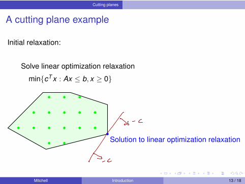
A cutting plane example
Initial relaxation:
Solve linear optimization relaxation
min{cT x : Ax b, x � 0}
Solution to linear optimization relaxation
Mitchell Introduction 13 / 18
¥- c

Cutting planes
A cutting plane example
Initial relaxation:
Solve linear optimization relaxation
min{cT x : Ax b, x � 0}
Solution to linear optimization relaxation
Cutting plane aT
1 x = b1
Mitchell Introduction 13 / 18
Cutting planes
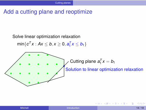
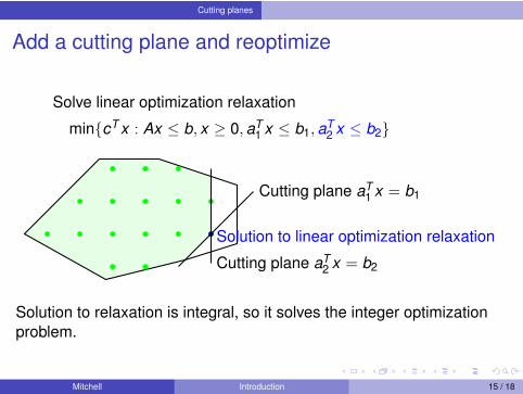
Add a cutting plane and reoptimize
Solve linear optimization relaxation
min{cT x : Ax b, x � 0, aT
1 x b1}
Solution to linear optimization relaxation
Cutting plane aT
1 x = b1
Mitchell Introduction 14 / 18
Cutting planes
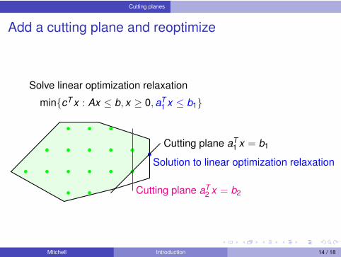
Add a cutting plane and reoptimize
Solve linear optimization relaxation
min{cT x : Ax b, x � 0, aT
1 x b1}
Solution to linear optimization relaxation
Cutting plane aT
1 x = b1
Cutting plane aT
2 x = b2
Mitchell Introduction 14 / 18
Cutting planes
Add a cutting plane and reoptimize
Solve linear optimization relaxation
min{cT x : Ax b, x � 0, aT
1 x b1, aT
2 x b2}
Solution to linear optimization relaxation
Cutting plane aT
1 x = b1
Cutting plane aT
2 x = b2
Solution to relaxation is integral, so it solves the integer optimizationproblem.
Mitchell Introduction 15 / 18
Branch-and-bound: An example
Outline
1 Integer and Combinatorial OptimizationComplexitySolution techniquesQuadratic constraints and objective functions
2 Cutting planes
3 Branch-and-bound: An example
Mitchell Introduction 16 / 18

Branch-and-bound: An example
An exampleWe look at the integer optimization problem
minx2R3 5x1 + 5x2 � 13x3subject to x1 + x2 + x3 6
10x1 � 8x2 15 (IOP)�6x1 � x2 + 9x3 9
xi � 0, xi integer, i = 1, 2, 3
It’s easy to find a feasible solution for this problem: x = (0, 0, 0).
Hence we can initialize with zu = 0.
We let
F = {x 2 R3 : x1 + x2 + x3 6, 10x1 � 8x2 15,�6x1 � x2 + 9x3 9,
x1, x2, x3 � 0}.
Mitchell Introduction 17 / 18

Branch-and-bound: An example
The tree for the example
Root node:min{c
Tx :
x 2 F}
x0 = (1.5, 0, 2),z
0 = �18.5
Mitchell Introduction 18 / 18

Branch-and-bound: An example
The tree for the example
Root node:min{c
Tx :
x 2 F}
x0 = (1.5, 0, 2),z
0 = �18.5
x2 = (2, 5
8 , 22972 ),
z2 = �18 1
9
x1 1x1 � 2
Mitchell Introduction 18 / 18

Branch-and-bound: An example
The tree for the example
Root node:min{c
Tx :
x 2 F}
x0 = (1.5, 0, 2),z
0 = �18.5
x1 = (1, 0, 1 2
3 ),z
1 = �16 23
x2 = (2, 5
8 , 22972 ),
z2 = �18 1
9
x1 1x1 � 2
Mitchell Introduction 18 / 18

Branch-and-bound: An example
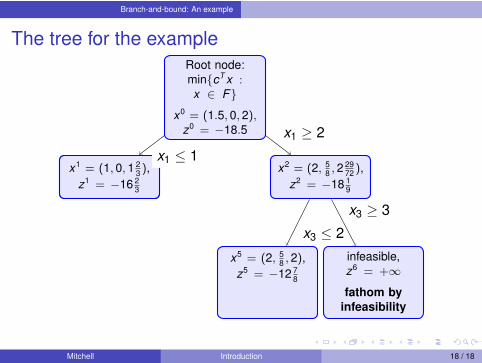
The tree for the exampleRoot node:min{c
Tx :
x 2 F}
x0 = (1.5, 0, 2),z
0 = �18.5
x1 = (1, 0, 1 2
3 ),z
1 = �16 23
x2 = (2, 5
8 , 22972 ),
z2 = �18 1
9
infeasible,z
6 = +1
fathom byinfeasibility
x1 1x1 � 2
x3 � 3
Mitchell Introduction 18 / 18
Branch-and-bound: An example
The tree for the exampleRoot node:min{c
Tx :
x 2 F}
x0 = (1.5, 0, 2),z
0 = �18.5
x1 = (1, 0, 1 2
3 ),z
1 = �16 23
x2 = (2, 5
8 , 22972 ),
z2 = �18 1
9
x5 = (2, 5
8 , 2),z
5 = �12 78
infeasible,z
6 = +1
fathom byinfeasibility
x1 1x1 � 2
x3 2x3 � 3
Mitchell Introduction 18 / 18

Branch-and-bound: An example
The tree for the exampleRoot node:min{c
Tx :
x 2 F}
x0 = (1.5, 0, 2),z
0 = �18.5
x1 = (1, 0, 1 2
3 ),z
1 = �16 23
x2 = (2, 5
8 , 22972 ),
z2 = �18 1
9
x3 = (0, 0, 1),z
3 = �13
fathom byintegrality
x5 = (2, 5
8 , 2),z
5 = �12 78
fathom bybounds
infeasible,z
6 = +1
fathom byinfeasibility
x1 1x1 � 2
x3 1 x3 2x3 � 3
Mitchell Introduction 18 / 18
¥*.
Branch-and-bound: An example
The tree for the exampleRoot node:min{c
Tx :
x 2 F}
x0 = (1.5, 0, 2),z
0 = �18.5
x1 = (1, 0, 1 2
3 ),z
1 = �16 23
x2 = (2, 5
8 , 22972 ),
z2 = �18 1
9
x3 = (0, 0, 1),z
3 = �13
fathom byintegrality
x4 = (1, 3, 2),z
4 = �6
fathom bybounds
x5 = (2, 5
8 , 2),z
5 = �12 78
fathom bybounds
infeasible,z
6 = +1
fathom byinfeasibility
x1 1x1 � 2
x3 1x3 � 2
x3 2x3 � 3
Mitchell Introduction 18 / 18

Branch-and-bound: An example
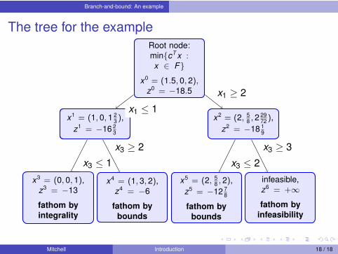
The tree for the exampleRoot node:min{c
Tx :
x 2 F}
x0 = (1.5, 0, 2),z
0 = �18.5
x1 = (1, 0, 1 2
3 ),z
1 = �16 23
x2 = (2, 5
8 , 22972 ),
z2 = �18 1
9
x3 = (0, 0, 1),z
3 = �13
fathom byintegrality
x4 = (1, 3, 2),z
4 = �6
fathom bybounds
x5 = (2, 5
8 , 2),z
5 = �12 78
fathom bybounds
infeasible,z
6 = +1
fathom byinfeasibility
x1 1x1 � 2
x3 1x3 � 2
x3 2x3 � 3
The optimal solution to (IOP) is x⇤ = (0, 0, 1), with value z⇤ = �13.Mitchell Introduction 18 / 18