chapter onestep metho ds - computer science | …flaherje/pdf/ode3.pdfsolution has form k n f t ch y...
TRANSCRIPT

Chapter �
One�Step Methods
��� Introduction
The explicit and implicit Euler methods for solving the scalar IVP
y� � f�t� y�� y��� � y�� �������
have an O�h� global error which is too low to make them of much practical value� With
such a low order of accuracy� they will be susceptible to round o� error accumulation�
Additionally� the region of absolute stability of the explicit Euler method is too small�
Thus� we seek higherorder methods which should provide greater accuracy than either
the explicit or implicit Euler methods for the same step size� Unfortunately� there is
generally a trade o� between accuracy and stability and we will typically obtain one at
the expense of the other�
Since we were successful in using Taylors series to derive a method� let us proceed
along the same lines� this time retaining terms of O�hk��
y�tn� � y�tn��� � hy��tn��� �h�
�y���tn��� � � � ��
hk
k y�k��tn��� �O�hk���� �������
Clearly� methods of this type will be explicit� Using �������
y��tn��� � f�tn��� y�tn����� ������a�
Di�erentiating �������
y���tn��� � �ft � fyy���tn���y�tn���� � �ft � fyf ��tn���y�tn����� ������b�
�

Continuing in the same manner
y����tn��� � �ftt � �ftyf � ftfy � fyyf� � f �
y f ��tn���y�tn����� ������c�
etc�
Speci�c methods are obtained by truncating the Taylors series at di�erent values of
k� For example� if k � � we get the method
yn � yn�� � hf�tn��� yn��� �h�
��ft � fyf ��tn�� �yn���� ������a�
From the Taylors series expansion �������� the local error of this method is
dn �h�
�y�����n�� ������b�
Thus� we succeeded in raising the order of the method� Unfortunately� methods of this
type are of little practical value because the partial derivatives are di�cult to evaluate
for realistic problems� Any software would also have to be problem dependent� By way
of suggesting an alternative� consider the special case of ������� when f is only a function
of t� i�e��
y� � f�t�� y��� � y��
This problem� which is of little interest� can be solved by quadrature to yield
y�t� � y� �
Z t
�
f���d��
We can easily construct highorder approximate methods for this problem by using nu
merical integration� Thus� for example� the simple leftrectangular rule would lead to
Eulers method� The midpoint rule with a step size of h would give us
y�h� � y� � hf�h��� �O�h���
Thus� by shifting the evaluation point to the center of the interval we obtained a higher
order approximation� Neglecting the local error term and generalizing the method to the
interval tn�� � t � tn yields
yn � yn�� � hf�tn�� � h����
�

Runge ���� sought to extend this idea to true di�erential equations having the form
of �������� Thus� we might consider
yn � yn�� � hf�tn � h��� yn�����
as an extension of the simple midpoint rule to �������� The question of how to de�ne
the numerical solution yn���� at the center of the interval remains unanswered� A simple
possibility that immediately comes to mind is to evaluate it by Eulers method� This
gives
yn���� � yn�� �h
�f�tn��� yn����
however� we must verify that this approximation provides an improved order of accuracy�
After all� Eulers method has an O�h�� local error and not an O�h�� error� Lets try to
verify that the combined scheme does indeed have an O�h�� local error by considering
the slightly more general scheme
yn � yn�� � h�b�k� � b�k��� ������a�
where
k� � f�tn��� yn���� ������b�
k� � f�tn�� � ch� yn�� � hak��� ������c�
Schemes of this form are an example of Runge�Kutta methods� We see that the proposed
midpoint scheme is recovered by selecting b� � �� b� � �� c � ���� and a � ���� We
also see that the method does not require any partial derivatives of f�t� y�� Instead� �the
potential� highorder accuracy is obtained by evaluating f�t� y� at an additional time�
The coe�cients a� b�� b�� and c will be determined so that a Taylors series expansion
of ������� using the exact ODE solution matches the Taylors series expansion �������
������ of the exact ODE solution to as high a power in h as possible� To this end� recall
the formula for the Taylors series of a function of two variables
F ��t� �� �y � �� � F ��t� �y� � ��Ft � �Fy���t��y� ��
��� �Ftt � ���Fty � ��Fyy���t��y� � � � �
�������
�

The expansion of ������� requires substitution of the exact solution y�t� into the formula
and the use of ������� to construct an expansion about �tn��� y�tn����� The only term
that requires any e�ort is k�� which� upon insertion of the exact ODE solution� has the
form
k� � f�tn�� � ch� y�tn��� � haf�tn��� y�tn������
To construct an expansion� we use ������� with F �t� y� � f�t� y�� �t � tn��� �y � y�tn����
� � ch� and � � haf�tn��� y�tn����� This yields
k� � f � chft � haffy ��
���ch��ftt � �ach�ffty � �ha��f �fyy� � O�h���
All arguments of f and its derivatives are �tn��� y�tn����� We have suppressed these to
simplify writing the expression�
Substituting the above expansion into ������a� while using ������b� with the exact
ODE solution replacing yn�� yields
y�tn� � y�tn��� � h�b�f � b��f � chft � haffy �O�h����� �������
Similarly� substituting ������� into �������� the Taylors series expansion of the exact
solution is
y�tn� � y�tn��� � hf �h�
��ft � ffy� �O�h��� �������
All that remains is a comparison of terms of the two expansions ������� and �������� The
constant terms agree� The O�h� terms will agree provided that
b� � b� � �� ������a�
The O�h�� terms of the two expansions will match if
cb� � ab� � ���� ������b�
A simple analysis would reveal that higher order terms in ������� and ������� cannot be
matched� Thus� we have three equations ������� to determine the four parameters a� b��
b�� and c� Hence� there is a one parameter family of methods and well examine two
speci�c choices�
�

�� Select b� � �� then a � c � ��� and b� � �� Using �������� this RungeKutta
formula is
yn � yn�� � hk� �������a�
with
k� � f�tn��� yn���� k� � f�tn�� � h��� yn�� � hk����� �������b�
Eliminating k� and k�� we can write �������� as
yn � yn�� � hf�tn�� � h��� yn�� � hf�tn��� yn������� �������a�
or
�yn���� � yn�� �h
�f�tn��� yn���� �������b�
yn � yn�� � hf�tn�� � h��� �yn������ �������c�
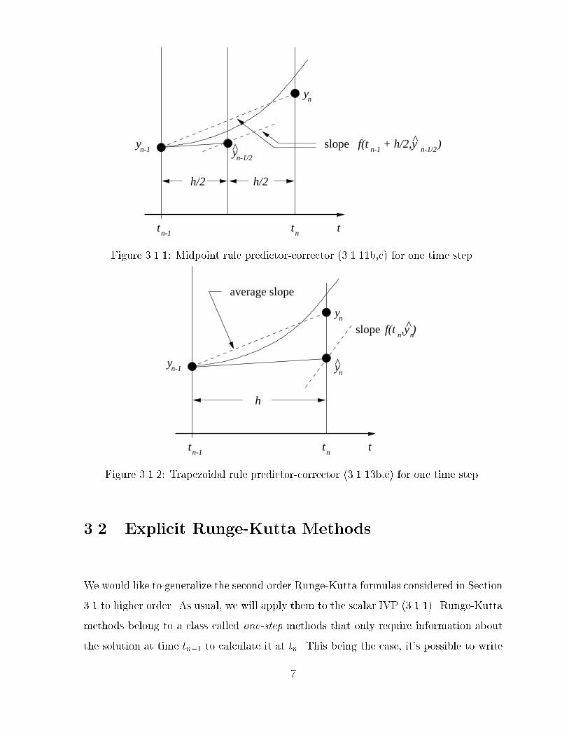
This is the midpoint rule integration formula that we discussed earlier� The � on
yn���� indicates that it is an intermediate rather than a �nal solution� As shown
in Figure ������ we can regard the twostage process �������b�c� as the result of two
explicit Euler steps� The intermediate solution �yn���� is computed at tn � h�� in
the �rst �predictor� step and this value is used to generate an approximate slope
f�tn � h��� �yn����� for use in the second �corrector� Euler step� According to Gear
����� this method has been called the EulerCauchy� improved polygon� Heun� or
modi�ed Euler method� Since there seems to be some disagreement about its name
and because of its similarity to midpoint rule integration� well call it the midpoint
rule predictorcorrector�
�� Select b� � ���� then a � c � � and b� � ���� According to �������� this Runge
Kutta formula is
yn � yn�� �h
��k� � k�� �������a�
�

with
k� � f�tn��� yn���� k� � f�tn�� � h� yn�� � hk��� �������b�
Again� eliminating k� and k��
yn � yn�� �h
��f�tn��� yn��� � f�tn� yn�� � hf�tn��� yn������ �������a�
This too� can be written as a twostage formula
�yn � yn�� � hf�tn��� yn���� �������b�
yn � yn�� �h
��f�tn��� yn��� � f�tn� �yn��� �������c�
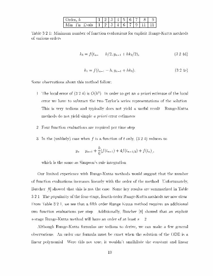
The formula �������a� is reminiscent of trapezoidal rule integration� The combined
formula �������b�c� can� once again� be interpreted as a predictorcorrector method�
Thus� as shown in Figure ������ the explicit Euler method is used to predict a
solution at tn and the trapezoidal rule is used to correct it there� Well call ��������
������� the trapezoidal rule predictorcorrector� however� it is also known as the
improved tangent� improved polygon� modi�ed Euler� or EulerCauchy method
������ Chapter ���
Using De�nition ������ we see that the Taylors series method ������� and the Runge
Kutta methods �������� and �������� are consistent to order two since their local errors
are all O�h�� �hence� their local discretization errors are O�h����
Problems
�� Solve the IVP
y� � f�t� y� � y � t� � �� y��� � ���
on � � t � � using the explicit Euler method and the midpoint rule� Use several
step sizes and compare the error at t � � as a function of the number of evaluations
of f�t� y�� The midpoint rule has twice the number of function evaluations of the
Euler method but is higher order� Which method is preferred�
�
t t t
y
n-1 n
n
yn-1/2
h/2 h/2
yn-1
slopen-1 n-1/2
f(t + h/2,y )^
Figure ������ Midpoint rule predictorcorrector �������b�c� for one time step�
t t t
y
n-1 n
n
yn-1
h
yn
^
slopen n
f(t ,y )^
average slope
Figure ������ Trapezoidal rule predictorcorrector �������b�c� for one time step�
��� Explicit Runge�Kutta Methods
We would like to generalize the second order RungeKutta formulas considered in Section
��� to higher order� As usual� we will apply them to the scalar IVP �������� RungeKutta
methods belong to a class called one�step methods that only require information about
the solution at time tn�� to calculate it at tn� This being the case� its possible to write
�

them in the general form
yn � yn�� � h��tn��� yn��� h�� �������
This representation is too abstract and well typically consider an sstage RungeKutta
formula for the numerical solution of the IVP ������� in the form
yn � yn�� � hsX
i��
biki� ������a�
where
ki � f�tn�� � cih� yn�� � hsX
j��
aijkj�� i � �� �� � � � � s� ������b�
These formulas are conveniently expressed as a tableau or a �Butcher diagram�
c� a�� a�� � � � a�sc� a�� a�� � � � a�s���
������
� � ����
cs as� as� � � � assb� b� � � � bs
or more compactly as
c A
b
We can also write ������� in the form
yn � yn�� � hsX
i��
bif�tn�� � cih� Yi�� ������a�
where
Yi � yn�� � hsX
j��
aijf�tn�� � cjh� Yj�� i � �� �� � � � � s� ������b�
In this form� Yi� i � �� �� � � � � s� are approximations of the solution at t � tn � cih that
typically do not have as high an order of accuracy as the �nal solution yn�
An explicit RungeKutta formula results when aij � � for j � i� Historically� all
RungeKutta formulas were explicit� however� implicit formula are very useful for sti�
systems and problems where solutions oscillate rapidly� Well study explicit methods in
this section and take up implicit methods in the next�
RungeKutta formulas are derived in the same manner as the secondorder methods
of Section ���� Thus� we
�

�� expand the exact solution of the ODE in a Taylors series about� e�g�� tn���
�� substitute the exact solution of the ODE into the RungeKutta formula and ex
panded the result in a Taylors series about� e�g�� tn��� and
�� match the two Taylors series expansions to as high an order as possible� The
coe�cients are usually not uniquely determined by this process� thus� there are
families of methods having a given order�
A RungeKutta method that is consistent to order k �or simply of order k� will match
the terms of order hk in both series� Clearly the algebra involved in obtaining these for
mulas increases combinatorically with increasing order� A symbolic manipulation system�
such as MAPLE or MATHEMATICA� can be used to reduce complexity� Fortunately�
the derivation is adequately demonstrated by the secondorder methods presented in
Section ��� and� for the most part� we will not need to present detailed derivations of
higherorder methods�
There are three oneparameter families of threestage� thirdorder explicit Runge
Kutta methods ��� ���� However� the most popular explicit methods are of order four�
Their tableau has the general form
� � � � �c� a�� � � �c� a�� a�� � �c a� a� a� �
b� b� b� b
The Taylors series produce eleven equations for the thirteen nonzero parameters listed
above� The classical RungeKutta method has the following form�
yn � yn�� �h
��k� � �k� � �k� � k�� ������a�
where
k� � f�tn��� yn���� ������b�
k� � f�tn�� � h��� yn�� � hk����� ������c�
�
Order� k � � � � � � � � �Min� Fn� Evals� � � � � � � � �� ��
Table ������ Minimum number of function evaluations for explicit RungeKutta methodsof various orders�
k� � f�tn�� � h��� yn�� � hk����� ������d�
k � f�tn�� � h� yn�� � hk��� ������e�
Some observations about this method follow�
�� The local error of ������� is O�h�� In order to get an a priori estimate of the local
error we have to subtract the two Taylors series representations of the solution�
This is very tedious and typically does not yield a useful result� RungeKutta
methods do not yield simple a priori error estimates�
�� Four function evaluations are required per time step�
�� In the �unlikely� case when f is a function of t only� ������� reduces to
yn � yn�� �h
��f�tn��� � �f�tn����� � f�tn���
which is the same as Simpsons rule integration�
Our limited experience with RungeKutta methods would suggest that the number
of function evaluations increases linearly with the order of the method� Unfortunately�
Butcher ��� showed that this is not the case� Some key results are summarized in Table
������ The popularity of the fourstage� fourthorder RungeKutta methods are now clear�
From Table ������ we see that a �fth order RungeKutta method requires an additional
two function evaluations per step� Additionally� Butcher ��� showed that an explicit
sstage RungeKutta method will have an order of at least s� ��
Although RungeKutta formulas are tedious to derive� we can make a few general
observations� An order one formula must be exact when the solution of the ODE is a
linear polynomial� Were this not true� it wouldnt annihilate the constant and linear
��

terms in a Taylors series expansion of the exact ODE solution and� hence� could not
have the requisite O�h�� local error to be �rstorder accurate� Thus� the RungeKutta
method should produce exact solutions of the di�erential equations y� � � and y� � ��
The constantsolution condition is satis�ed identically by construction of the Runge
Kutta formulas� Using ������a�� the latter �linearsolution� condition with y�t� � t and
f�t� y� � � implies
tn � tn�� � hsX
i��
bi
or
sXi��
bi � �� ������a�
If we also require the intermediate solutions Yi to be �rst order� then the use of ������b�
with Yi � tn�� � cih gives
ci �sX
j��
aij� i � �� �� � � � � s� ������b�
This condition does not have to be satis�ed for loworder RungeKutta methods �����
however� its satisfaction simpli�es the task of obtaining order conditions for higherorder
methods� Methods that satisfy ������b� also treat autonomous and nonautonomous
systems in a symmetric manner �Problem ���
We can continue this process to higher orders� Thus� the RungeKutta method will
be of order p if it is exact when the di�erential equation and solution are
y� � �t� tn���l��� y�t� �
�
l�t� tn���
l� l � �� �� � � � � p�
�The use of t � tn�� as a variable simpli�es the algebraic manipulations�� Substituting
these solutions into ������a� implies that
hl
l� h
sXj��
bi�cih�l��
or
sXi��
bicl��i �
�
l� l � �� �� � � � � p� ������c�
��

Conditions ������c� are necessary for a method to be order p� but may not be su�cient�
Note that there is no dependence on the coe�cients aij i� j � �� �� � � � � s� in formulas
������a�c�� This is because our strategy of examining simple di�erential equations is
not matching all possible terms in a Taylors series expansion of the solution� This� as
noted� is a tedious operation� Butcher developed a method of simplifying the work by
constructing rooted trees that present the order conditions in a graphical way� They
are discussed in many texts �e�g�� ���� ����� however� they are still complex and we will
not pursue them here� Instead� well develop additional necessary order conditions by
considering the simple ODE
y� � y�
Replacing f�t� y� in ������� by y yields
yn � yn�� � hsX
i��
biYi�
Yi � yn�� � hsX
j��
aijYj� i � �� �� � � � � s�
Its simpler to use vector notation
yn � yn�� � hbTY� Y � yn��l� hAY
where
Y � �Y�� Y�� � � � � Ys�T � ������a�
l � ��� �� � � � � ��T � ������b�
A �
�����a�� a�� � � � a�sa�� a�� � � � a�s���
���� � �
���as� as� � � � ass
����� � ������c�
and
b � �b�� b�� � � � � bs�T � ������d�
��

Eliminating Y� we have
Y � yn���I� hA���l
and
yn � yn�� � hyn��bT �I� hA���l�
Assuming that yn�� is exact� the exact solution of this test equation is yn � ehyn���
Expanding this solution and �I� hA��� in series
� � h� � � ��hk
k � � � � � � � hbT �I� hA� � � �� hkAk � � � � �l�
Equating like powers of h yields the order condition
bTAk��l ��
k � k � �� �� � � � � p� �������
We recognize that this condition with k � � is identical to ������a�� Letting c �
�c�� c�� � � � � cs�T � we may write ������c� with l � � in the form bTc � ���� The
vector form of ������b� is Al � c� Thus� bTAl � ���� which is the same as ������� with
k � �� Beyond k � �� the order conditions ������c� and ������� are independent�
Although conditions ������� and ������� are only necessary for a method to be of order
p� they are su�cient in many cases� The actual number of conditions for a RungeKutta
method of order p are presented in Table ����� ����� These results assume that ������b�
has been satis�ed�
Order� p � � � � � � � � � ��No� of Conds� � � � � �� �� �� ��� ��� ����
Table ������ The number of conditions for a RungeKutta method of order p �����
Theorem ������ The necessary and su�cient conditions for a Runge�Kutta method
������� to be of second order are ������c�� l � �� �� and ������� k � �� If ������b� is
satised then �������� k � �� �� are necessary and su�cient for second�order accuracy�
Proof� We require numerous Taylors series expansions� To begin� we expand f�tn�� �
cih� Yi� using ������� to obtain
f�tn�� � cih� Yi� � f � ftcih� fy�Yi � y�tn���� ��
��ftt�cih�
� � �fty�cih��Yi � y�tn�����
��

fyy�Yi � y�tn������ �O�h���
All arguments of f and its derivatives are at �tn��� y�tn����� They have been suppressed
for simplicity�
Substituting the exact ODE solution and the above expression into ������a� yields
y�tn� � y�tn��� � hsX
i��
bi�f � ftcih� fy�Yi � y�tn���� �O�h����
The expansion of Yi�y�tn��� will� fortunately� only require the leading term� thus� using
������b�
Yi � y�tn��� � hsX
j��
aijf �O�h���
Hence� we have
y�tn� � y�tn��� � hsX
i��
bi�f � ftcih� hffy
sXj��
aij �O�h����
Equating terms of this series with the Taylors series ������� of the exact solution yields
������c� with l � �� ������c� with l � �� and ������� with k � �� We have demonstrated
the equivalence of these conditions when ������b� is satis�ed�
Remark �� The results of Theorem ����� and conditions ������� and ������� apply to
both explicit and implicit methods�
Let us conclude this section with a brief discussion of the absolute stability of explicit
methods� We will present a more detailed analysis in Section ���� however� the present
material will serve to motivate the need for implicit methods� Thus� consider an sstage
explicit RungeKutta method applied to the test equation
y� � �y� �������
Using ������� in ������� with the simpli�cation that aij � �� j � i� for explicit methods
yields
yn � yn�� � zsX
i��
biYi � yn�� � zbTY ������a�
��

where
Yi � yn�� � zi��Xj��
aijYj� i � �� �� � � � � s� ������b�
and
z � h�� ������c�
The vector form of ������� is
Y � yn��l� zAY� ������d�
Using this to eliminate Y in ������a�� we have
yn � yn���� � zbT �I� zA���l��
Expanding the inverse
yn � yn���� � zbT �I� zA� � � �� zkAk � � � � �l�
Using �������
yn � R�z�yn�� �������a�
where
R�z� � � � z �z�
�� � � ��
zp
p �
�Xj�p��
zjbTAj��l�
The matrix A is strictly lower triangular for an sstage explicit RungeKutta method�
thus� Aj�� � �� j s� Therefore�
R�z� � � � z �z�
�� � � ��
zp
p �
sXj�p��
zjbTAj��l� �������b�
In particular� for explicit sstage methods with p � s � �� we have
R�z� � � � z �z�
�� � � ��
zp
p � s � p � �� �������c�
The exact solution of the test equation ������� is
y�tn� � eh�y�tn����
��

thus� as expected� a pthorder RungaKutta formula approximates a Taylors series ex
pansion of the exact solution through terms of order p�
Using De�nition ����� and ��������� the region of absolute stability of an explicit
RungeKutta method is
jR�z�j ������� � z �
z�
�� � � ��
zp
p �
sXj�p��
zjbTAj��l
����� � �� �������a�
In particular�
jR�z�j ������ � z �
z�
�� � � ��
zp
p
���� � �� s � p � �� �������b�
Since no RungeKutta coe�cients appear in �������b�� we have the interesting result�
Lemma ������ All p�stage explicit Runge�Kutta methods of order p � � have the same
region of absolute stability�
Since jei�j � �� � � � ��� we can determine the boundary of the absolute stability
regions �������a�b� by solving the nonlinear equation
R�z� � ei�� ��������
Clearly� �������� implies that jyn�yn��j � �� For p � � �i�e�� for Eulers method�� the
boundary of the absolutestability region is determined as
� � z � ei��
which can easily be recognized as the familiar unit circle centered at z � �� � �i� For
real values of z the intervals of absolute stability for methods with p � s � � are shown
in Table ������ Absolute stability regions for complex values of z are illustrated for the
same methods in Figure ������ Methods are stable within the closed regions shown� The
regions of absolute stability grow with increasing p� When p � �� �� they also extend
slightly into the right half of the complex zplane�
Problems
�� Instead of solving the IVP �������� many software systems treat an autonomous
ODE y� � f�y�� Nonautonomous ODEs can be written as autonomous systems
��

Order� p Interval ofAbsolute Stability
� ������ ������ ��������� ��������
Table ������ Interval of absolute stability for pstage explicit RungeKutta methods oforder p � �� �� �� ��
−5 −4 −3 −2 −1 0 1−3
−2
−1
0
1
2
3
Re(z)
Im(z)
Figure ������ Region of absolute stability for pstage explicit RungeKutta methods oforder p � �� �� �� � �interiors of smaller closed curves to larger ones��
��

by letting t be a dependent variable satisfying the ODE t� � �� A RungeKutta
method for an autonomous ODE can be obtained from� e�g�� ������� by dropping
the time terms� i�e��
yn � yn�� � hsX
i��
bif�Yi��
with
Yi � yn�� � hsX
j��
aijf�Yj�� i � �� �� � � � � s�
The RungeKutta evaluation points ci� i � �� �� � � � � s� do not appear in this form�
Show that RungeKutta formulas ������� and the one above will handle autonomous
and nonautonomous systems in the same manner when ������b� is satis�ed�
��� Implicit Runge�Kutta Methods
Well begin this section with a negative result that will motivate the need for implicit
methods�
Lemma ������ No explicit Runge�Kutta method can have an unbounded region of abso�
lute stability�
Proof� Using ��������� the region of absolute stability of an explicit RungeKutta method
satis�es
jyn�yn��j � jR�z�j � �� z � h��
where R�z� is a polynomial of degree s� the number of stages of the method� Since R�z�
is a polynomial� jR�z�j � � as jzj � � and� thus� the stability region is bounded�
Hence� once again� we turn to implicit methods as a means of enlarging the region of
absolute stability�
Necessary order conditions for sstage implicit RungeKutta methods are given by
������c� ������ �with su�cient conditions given in Hairer et al� ����� Section II���� A
condition on the maximum possible order follows�
Theorem ������ The maximum order of an implicit s�stage Runge�Kutta method is �s�
��

Proof� cf� Butcher ����
The derivations of implicit RungeKutta methods follow those for explicit methods�
Well derive the simplest method and then give a few more examples�
Example ������ Consider the implicit �stage method obtained from ������� with s � �
as
yn � yn�� � hb�f�tn�� � c�h� Y��� ������a�
Y� � yn�� � ha��f�tn�� � c�h� Y��� ������b�
To determine the coe�cients c�� b�� and a��� we substitute the exact ODE solution into
������a�b� and expand ������a� in a Taylors series
y�tn� � y�tn��� � hb��f � c�hft � fy�Y� � y�tn���� �O�h����
where f �� f�tn��� y�tn����� etc� Expanding ������b� in a Taylors series and substituting
the result into the above expression yields
y�tn� � y�tn��� � hb��f � c�hft � ha��ffy �O�h����
Comparing the terms of the above series with the Taylors series
y�tn� � y�tn��� � hf �h�
��ft � ffy� �O�h��
of the exact solution yields
b� � �� a�� � c� ��
��
Substituting these coe�cients into �������� we �nd the method to be an implicit midpoint
rule
yn � yn�� � hf�tn�� � h��� Y��� ������a�
Y� � yn�� �h
�f�tn�� � h��� Y��� ������b�
The tableau for this method is
��

��
��
�
The formula has similarities to the midpoint rule predictorcorrector ��������� however�
there are important di�erences� Here� the backward Euler method �rather than the
forward Euler method� may be regarded as furnishing a predictor ������b� with the
midpoint rule providing the corrector ������a�� However� formulas ������a� and ������b�
are coupled and must be solved simultaneously rather than sequentially�
Example ������ The twostage method having maximal order four presented in the
following tableau was developed by Hammer and Hollingsworth �����
���
p��
�
��
p��
���
p��
��
p��
�
��
��
This method is derived in Gear ����� Section ����
Example ������ Let us examine the region of absolute stability of the implicit midpoint
rule �������� Thus� applying ������� to the test equation ������� we �nd
Y� � yn�� �h�
�Y�
and
yn � yn�� � h�Y��
Solving for Y�
Y� �yn��
�� h����
and eliminating it in order to explicitly determine yn as
yn �
�� �
h�
�� h���
�yn�� �
�� � h���
�� h���
�yn���
Thus� the region of absolute stability is interior to the curve
� � z��
�� z��� ei�� z � h��
Solving for z
z � ��� ei�
� � ei�� ��e
i��� � e�i���
ei��� � e�i���� ��i tan ���
��

λ)Re(h
Im(h λ)
Figure ������ Region of absolute stability for the implicit midpoint rule ��������
Since z is imaginary� the implicit midpoint rule is absolutely stable in the entire negative
half of the complex z plane �Figure �������
Let us generalize the absolute stability analysis presented in Example ����� before
considering additional methods� This analysis will be helpful since we will be interested
in developing methods with very large regions of absolute stability� Thus� we apply the
general method ������� to the test equation ������� to obtain
yn � yn�� � zbTY� ������a�
�I� zA�Y � yn��l� ������b�
where Y� l� A� and b and are de�ned by ������� and z � h��
Eliminating Y in ������a� by using ������b� we �nd
yn � R�z�yn��� ������a�
where
R�z� � � � zbT �I� zA���l� ������b�
The region of absolute stability is the set of all complex z where jR�z�j � �� While R�z�
is a polynomial for an explicit method� it is a rational function for an implicit method�
��

Hence� the region of absolute stability can be unbounded� As shown in Section ���� a
method of order p will satisfy
R�z� � ez �O�zp����
Rationalfunction approximations of the exponential are called Pad�e approximations�
De�nition ������ The �j� k� Pad�e approximation Rjk�z� is the maximum�order approx�
imation of ez having the form
Rjk�z� �Pk�z�
Qj�z��
p� � p�z � � � �� pkzk
q� � q�z � � � �� qjzj� ������a�
where Pk and Qj have no common factors�
Qj��� � q� � �� ������b�
and
Rjk�z� � ez �O�zk�j���� ������c�
With Rjk normalized by ������b�� there are k � j � � undetermined parameters in
������a� that can be determined by matching the �rst k � j � � terms in the Taylors
series expansion of ez� Thus� the error of the approximation should be O�zk�j���� Using
������c�� we have
k�jXi��
zi
i �
Pki�� piz
iPji�� qiz
i�O�zk�j��� �������
Equating the coe�cients of like powers of z determines the parameters pi� i � �� �� � � � � k
and qi� i � �� �� � � � � j�
Example ���� � Find the ����� Pad�e approximation of ez� Setting j � � and k � � in
������� gives
�� � z �z�
���� � q�z � q�z
�� � p��
Equating the coe�cients of zi� i � �� �� �� gives
p� � �� � � q� � ���
�� q� � q� � ��
��

Thus�
p� � �� q� � ��� q� � ����
Using �������� the ����� Pad�e approximation is
R���z� ��
�� z � z����
Additionally�
ez � R���z� �O�z���
Some other Pad�e approximations are presented in Table ������ We recognize that
the ����� approximation corresponds to Eulers method� the ����� method corresponds
to the backward Euler method� and the ����� approximation corresponds to the mid
point rule� �The ����� approximation also corresponds to the trapezoidal rule�� Methods
corresponding to the �s� s� diagonal Pad�e approximations are Butchers maximum order
implicit RungeKutta methods �Theorem �������
k � � � �j � � � � � z � � z � z���
� ���z
��z����z��
���z���z�����z��
� ���z�z���
��z�����z���z���
��z���z������z���z����
Table ������ Some Pad�e approximations of ez�
Theorem ������ There is one and only one �s�order s�stage implicit Runge�Kutta for�
mula and it corresponds to the �s� s� Pad�e approximation�
Proof� cf� Butcher ����
Well be able to construct several implicit RungeKutta methods having unbounded
absolutestability regions� Well want to characterize these methods according to their
behavior as jzj � � and this requires some additional notions of stability�
De�nition ������ A numerical method is A�stable if its region of absolute stability in�
cludes the entire left�half plane Re�h�� � ��
��

The relationship between Astability and the Pad�e approximations is established by
the following theorem�
Theorem ������ Methods that lead to a diagonal or one of the rst two sub�diagonals
of the Pad�e table for ez are A�stable�
Proof� The proof appears in Ehle ����� Without introducing additional properties of Pad�e
approximations� well make some observations using the results of Table ������
�� We have shown that the regions of absolute stability of the backward Euler method
and the midpoint rule include the entire lefthalf of the h� plane� hence� they are
Astable�
�� The coe�cients of the highestorder terms of Ps�z� and Qs�z� are the same for
diagonal Pad�e approximations Rss�z�� hence� jRss�z�j � � as jzj � � and these
methods are Astable �Table �������
�� For the subdiagonal ����� and ����� Pad�e approximations� jR�z�j � � as jzj � �and these methods will also be Astable�
It is quite di�cult to �nd highorder Astable methods� Implicit RungeKutta meth
ods provide the most viable approach� Examining Table ������ we see that we can intro
duce another stability notion�
De�nition ������ A numerical method is L�stable if it is A�stable and if jR�z�j � � as
jzj � ��
The backward Euler method and� more generally� methods corresponding to sub
diagonal Pad�e approximations in the �rst two bands are Lstable ������ Section IV����
Lstable methods are preferred for sti� problems where Re��� � � but methods where
jR�z�j � � are more suitable when Re��� � � but jIm���j � �� i�e�� when solutions
oscillate rapidly�
Explicit RungeKutta methods are easily solved� but implicit methods will require
an iterative solution� Since implicit methods will generally be used for sti� systems�
��

Newtons method will be preferred to functional iteration� To emphasize the di�culty�
well illustrate RungeKutta methods of the form ������� for vector IVPs
y� � f�t�y�� y��� � y�� �������
where y� etc� are mvectors� The application of ������� to vector systems just requires
the use of vector arithmetic� thus�
Yi � yn�� � hsX
j��
aijf�tn�� � cjh�Yj�� i � �� �� � � � � s� ������a�
yn � yn�� � hsX
i��
bif�tn�� � cih�Yi�� ������b�
Once again� yn etc� are mvectors�
To use Newtons method� we write the nonlinear system ������a� in the form
Fi�Y��Y�� � � � �Ys� � Yi � yn�� � hsX
j��
aijf�tn�� � hcj�Yj� � �� j � �� �� � � � � s�
������a�
and get
�����I� a��J
���� �ha��J���
� �ha�sJ���s
�ha��J���� I� ha��J
���� �ha�sJ���
s
������
� � ����
�has�J���� �has�J���
� I� hassJ���s
�����������Y
����
�Y�������
�Y���s
����� � �
�����F
����
F�������
F���s
����� � ������b�
Y�����i � Y
���i � �Y���
i � i � �� �� � � � � s� � �� �� � � � � ������c�
where
J���j � fy�tn�� � hcj�Y
���j �� F
���j � Fj�Y
���� �Y
���� � � � � �Y���
s �� j � �� �� � � � � s�
������d�
For an sstage RungeKutta method applied to an mdimensional system ��������
the Jacobian in ������b� has dimension sm sm� This will be expensive for highorder
methods and highdimensional ODEs and will only be competitive with� e�g�� implicit
��

multistep methods �Chapter �� under special conditions� Some simpli�cations are possi
ble and these can reduce the work� For example� we can approximate all of the Jacobians
as
J � fy�tn���yn���� �������a�
In this case� we can even shorten the notation by introducing the Kronecker or direct
product of two matrices as
A J �
�����a��J a��J a�sJa��J a��J a�sJ���
���� � �
���as�J as�J assJ
����� � �������b�
Then� ������b� can be written concisely as
�I� hA J��Y��� � �F��� �������c�
where A was given by ������c� and
�Y��� �
������Y
����
�Y�������
�Y���s
����� � F��� �
�����F
����
F�������
F���s
����� � �������d�
The approximation of the Jacobian does not change the accuracy of the computed solu
tion� only the convergence rate of the iteration� As long as convergence remains good�
the same Jacobian can be used for several time step and only be reevaluated when
convergence of the Newton iteration slows�
Even with this simpli�cation� with m ranging into the thousands� the solution of
�������� is clearly expensive and other ways of reducing the computational cost are nec
essary� Diagonally implicit Runge�Kutta �DIRK� methods o�er one possibility� A DIRK
method is one where aij � �� i � j and at least one aii �� �� i� j � �� �� � � � � s� If� in
addition� a�� � a�� � � � � � ass � a� the technique is known as a singly diagonally implicit
Runge�Kutta �SDIRK� method� Thus� the coe�cient matrix of an SDIRK method has
��

the form
A �
�����
aa�� a���
���� � �
as� as� a
����� � ��������
Thus� with the approximation ��������� the system Jacobian in �������c� is
�I� hA J� �
�����I� haJ ��ha��J I� haJ �
������
� � ����
�has�J �has�J I� haJ
����� �
The Newton system �������� is lower block triangular and can be solved by forward
substitution� Thus� the �rst block of �������c� is solved for �Y���� � Knowing Y� the
second equation is solved for �Y���� � etc� The Jacobian J is the same for all stages� thus�
the diagonal blocks need only be factored once by Gaussian elimination and forward and
backward substitution may be used for each solution�
The implicit midpoint rule ������� is a onestage� secondorder DIRK method� Well
examine a twostage DIRK method momentarily� but �rst we note that the maximum
order of an sstage DIRK method is s� � ����
Example ������ A twostage DIRK formula has the tableau
c� a�� �c� a�� a��
b� b�
and it could be of third order� According to Theorem ������ the conditions for second
order accuracy are ������c� with l � �� � when ������b� is satis�ed� i�e��
b� � b� � �� c� � a��� c� � a�� � a��� b�c� � b�c� � ����
�As noted earlier� satisfaction of ������b� is not necessary� but it simpli�es the algebraic
manipulations�� We might guess that the remaining conditions necessary for third order
accuracy are ������c� with l � � and ������� with k � �� i�e��
b�c�� � b�c
�� � ���
and
bTA�l � bAc � b�a��c� � b��a��c� � a��c�� � ����
��

where ������b� was used to simplify the last expression� After some e�ort� this system of
six equations in seven unknowns can be solved to yield
c� ��� �c��� �c�
� b� �c� � ���
c� � c�� b� �
���� c�c� � c�
�
a�� � c�� a�� ����� b�c
��
b��c� � c��� a�� � c� � a���
As written� the solution is parameterized by c�� Choosing c� � ��� gives
� � � � �� � � � �
� � � �
Using �������� the method is
Y� � yn�� �h
�f�tn�� �
h
�� Y��� Y� � yn�� �
h
��f�tn�� �
h
�� Y�� � f�tn� Y����
yn � yn�� �h
���f�tn�� �
h
�� Y�� � f�tn� Y����
We can check by constructing a Taylors series that this method is indeed third order�
Hairer et al� ����� Section II��� additionally show that our necessary conditions for third
order accuracy are also su�cient in this case�
The computation of Y� can be recognized as the backward Euler method for onethird
of the time step h� The computation of Y� and yn are not recognizable in terms of simple
quadrature rules� Since the method is thirdorder� its local error is O�h��
We can also construct an SDIRK method by insisting that a�� � a��� Enforcing this
condition and using the previous relations gives two methods having the tableau
� � ��� � �� �� �
��� ���
where
� ��
���� �p
���
The method with � � �� � ��p���� is Astable while the other method has a bounded
stability region� Thus� this would be the method of choice�
��

Let us conclude this Section by noting a relationship between implicit RungeKutta
and collocationmethods� With u�t� a polynomial of degree s in t for t � tn��� a collocation
method for the IVP
y� � f�t� y�� y�tn��� � yn�� �������a�
consists of solving
u�tn��� � yn�� �������b�
u��tn�� � cih� � f�tn�� � cih� u�tn�� � cih��� i � �� �� � � � � s� �������c�
where ci� i � �� �� � � � � s� are nonnegative parameters� Thus� the collocation method
consists of satisfying the ODE exactly at s points� The solution u�tn���h� may be used
as the initial condition yn for the next time step�
Usually� the collocation points tn�� � cih are such that ci ��� ��� i � �� �� � � � � s� but
this need not be the case ��� ��� ����
Generally� the ci� i � �� �� � � � � s� are distinct and we shall assume that this is the case
here� �The coe�cients need not be distinct when the approximation u�t� interpolates
some solution derivatives� e�g�� as with Hermite interpolation�� Approximating u��t��
t � tn��� by a Lagrange interpolating polynomial of degree s� �� we have
u��t� �sX
j��
kjLj�t� tn��
h� �������a�
where
Lj��� �sY
i���i��j
� � cicj � ci
� �������b�
� �t� tn��
h� �������c�
The polynomials Lj���� j � �� �� � � � � s� are a product of s � � linear factors and are�
hence� of degree s� �� They satisfy
Lj�ci� � �ji� j� i � �� �� � � � � s� �������d�
��

where �ji is the Kronecker delta� Using �������a�� we see that u��t� satis�es the interpo
lation conditions
u��tn�� � cih� � ki� i � �� �� � � � � s� �������e�
Transforming variables in �������a� using �������c�
u�tn�� � �h� � yn�� � h
Z �
�
u��tn�� � �h�d�� ��������
By construction� �������� satis�es �������b�� Substituting �������e� and �������� into
�������c�� we have
ki � f�tn�� � cih� yn�� � h
sXj��
kj
Z ci
�
Lj���d���
This formula is identical to the typical RungeKutta formula ������b� provided that
aij �
Z ci
�
Lj���d�� �������a�
Similarly� using �������a� in �������� and evaluating the result at � � � yields
u�tn�� � h� � yn � yn�� � hsX
j��
kj
Z �
�
Lj���d��
This formula is identical to ������a� provided that
bj �
Z �
�
Lj���d�� �������b�
This view of a RungeKutta method as a collocation method is useful in many situations�
Let us illustrate one result�
Theorem ������ A Runge�Kutta method with distinct ci� i � �� �� � � � � s� and of order
at least s is a collocation method satisfying ��������� �������� if and only if it satises
the order conditions
sXj��
aijcq��j �
cqiq� i� q � �� �� � � � � s� ��������
Remark �� The order conditions �������� are related to the previous conditions ������c�
������ �cf� ����� Section II����
��

Proof� We use the Lagrange interpolating polynomial �������� to represent any polyno
mial P ��� of degree s� � as
P ��� �sX
j��
P �cj�Lj����
Regarding P ��� as u��tn � �h�� integrate to obtain
u�tn�� � cih�� yn�� �Z ci
�
P ���d� �sX
j��
P �cj�
Z ci
�
Lj���d�� i � �� �� � � � � s�
Assuming that �������a� is satis�ed� we haveZ ci
�
P ���d� �sX
j��
aijP �cj�� i � �� �� � � � � s�
Now choose P ��� � � q��� q � �� �� � � � � s� to obtain ��������� The proof of the converse
follows the same arguments �cf� ����� Section II����
Now� we might ask if there is an optimal way of selecting the collocation points� Ap
propriate strategies would select them so that accuracy and or stability are maximized�
Lets handle accuracy �rst� The following theorems discuss relevant accuracy issues�
Theorem ������ �Alekseev and Gr�obner� Let x� y� and z satisfy
x��t� �� z���� � f�t� x�t� �� z������ x��� �� z���� � z���� �������a�
y��t� � f�t� y�t��� y��� � y�� �������b�
z��t� � f�t� z�t�� � g�t� z�t��� z��� � y�� �������c�
with fy�t� y� C�� t �� Then�
z�t�� y�t� �
Z t
�
�x�t� �� z����
�zg��� z����d�� �������d�
Remark �� Formula �������d� is often called the nonlinear variation of parameters�
Remark �� The parameter � identi�es the time that the initial conditions are applied
in �������a�� A prime� as usual� denotes t di�erentiation�
Remark � Observe that y�t� � x�t� �� y���
��

Proof� cf� Hairer et al� ����� Section I���� and Problem ��
Theorem ����� makes it easy for us to associate the collocation error with a quadrature
error as indicated below�
Theorem ������ Consider the quadrature ruleZ tn
tn��
F �t�dt � h
Z �
�
F �tn�� � �h�d� � hsX
i��
biF �tn�� � cih� � Ep �������a�
where
Ep � Chp��F �p���n�� �n �tn��� tn�� �������b�
F Cp�tn��� tn�� and C is a constant� Then the collocation method �������� has order p�
Proof� Consider the identity
u� � f�t� u� � �u� � f�t� u��
and use Theorem ����� on �tn��� tn� with z�t� � u�t� and g�t� u� � u� � f�t� u� to obtain
u�tn�� y�tn� �
Z tn
tn��
xu�tn� �� u�����u����� f��� u�����d��
Replace this integral by the quadrature rule �������� to obtain
u�tn�� y�tn� � hsX
i��
bixu�tn� tn�� � cih� u�tn�� � cih���u��tn�� � cih��
f�tn�� � cih� u�tn�� � cih��� � Ep�
All terms in the summation vanish upon use of the collocation equations ��������� thus�
ju�tn�� y�tn�j � jEpj � jCjhp�� max���tn�� �tn
j �p
��pxu�tn� �� u�����u
����� f��� u��j�
It remains to show that the derivatives in the above expression are bounded as h � ��
Well omit this detail which is proven in Hairer et al� ����� Section II��� Thus�
jy�tn�� u�tn�j � �Chp�� ��������
and the collocation method �������� is of order p�
��

At last� our task is clear� We should select the collocation points ci� i � �� �� � � � � s�
to maximize the order p of the quadrature rule ��������� Well review some of the details
describing the derivation of ��������� Additional material appears in most elementary
numerical analysis texts ���� Let �F ��� � F �tn�� � �h� and approximate it by a Lagrange
interpolating polynomial of degree s� � to obtain
�F ��� �sX
j��
�F �cj�Lj��� �Ms���
s �F �s����� � ��� ��� �������a�
where
Ms��� �sY
i��
�� � ci�� �������b�
�Di�erentiation in �������a� is with respect to � � not t��
Integrate �������a� and use �������b� to obtain
Z �
�
�F ���d� �sX
j��
bj �F �cj� � �Es �������a�
where
�Es ��
s
Z �
�
Ms��� �F�s�������d� �
�
s
Z �
�
sYi��
�� � ci� �F�s�������d�� �������b�
In NewtonCotes quadrature rules� such as the trapezoidal and Simpsons rules� the
evaluation points ci� i � �� �� � � � � s� are speci�ed a priori� With Gaussian quadrature�
however� the points are selected to maximize the order of the rule� This can be done by
expanding �F �s������� in a Taylors series and selecting the ci� i � �� �� � � � � s� to annihilate
as many terms as possible� Alternatively� and equivalently� the quadrature rule can be
designed to integrate polynomials exactly to as high a degree as possible� The actual
series expansion is complicated by the fact that �F �s� is evaluated at ���� in �������b��
Isaacson and Keller ���� provide additional details on this matter� however� well sidestep
the subtleties by assuming that all derivatives of ���� are bounded so that �F �s� has an
expansion in powers of � of the form
�F �s���� � �� � ��� � � � �� �r���r�� �O�� r��
��

d Pd�x�
� �
� x
� x� � ��
� x� � �x
� x � �x�
�� �
�
� x � ��x�
�� x
��
Table ������ Legendre polynomials Pd�x� of degree d ��� �� on �� � x � ��
The �rst r terms of this series will be annihilated by �������b� if Ms��� is orthogonal
to polynomials of degree r � �� i�e�� ifZ �
�
M���� q��d� � �� q � �� �� � � � � r� ��������
Under these conditions� were we to transform the integrals in �������� and �������� back
to t dependence using �������c�� we would obtain the error of �������b� with p � s � r�
With the s coe�cients ci� i � �� �� � � � � s� we would expect the maximum value of r to
be s� According to Theorem ������ this choice would lead to a collocation method of
order �s� i�e�� a method having p � r � s � �s and an O�h�s��� local error� These are
Butchers maximal order formulas �Theorem ������ corresponding to the diagonal Pad�e
approximations�
The maximumorder coe�cients identi�ed above are the roots of the s thdegree
Legendre polynomial scaled to the interval ��� ��� The �rst six Legendre polynomials are
listed in Table ������ Additional polynomials and their roots appear in Abromowitz and
Stegun ���� Chapter ���
Example ������ According to Table ������ the roots of P��x� are x��� � ���p� on
���� ��� Mapping these to ��� �� by the linear transformation � � �� � x���� we obtain
the collocation points for the maximalorder twostage method as
c� ��
���� �p
��� c� �
�
��� �
�p���
��

Since this is our �rst experience with these techniques� let us verify our results by a direct
evaluation of �������� using �������b�� thus�Z �
�
�� � c���� � c��d� � ��
Z �
�
�� � c���� � c���d� � ��
Integrating�
�� c� � c�
�� c�c� � ��
�
�� c� � c�
��c�c��
� ��
These may easily be solved to con�rm the collocation points obtained by using the roots
of P��x�� In this case� we recognize c� and c� as the evaluation points of the Hammer
Hollingsworth formula of Example ������
With the collocation points ci� i � �� �� � � � � s� determined� the coe�cients aij and bj�
i� j � �� �� � � � � s� may be determined from �������a�b�� These maximal order collocation
formulas are Astable since they correspond to diagonal Pad�e approximations �Theorem
�������
We may not want to impose the maximal order conditions to obtain� e�g�� better
stability and computational properties� With Radau quadrature� we �x one of the coef
�cients at an endpoint� thus� we set either c� � � or cs � �� The choice c� � � leads to
methods with bounded regions of absolute stability� Thus� the methods of choice have
cs � �� They correspond to the subdiagonal Pad�e approximations and are� hence� A
and Lstable �Theorem ������� They have orders of p � �s � � ����� Section IV��� Such
excellent stability and accuracy properties makes these methods very popular for solving
sti� systems�
The Radau polynomial of degree s on �� � x � � is
Rs�x� � Ps�x�� s
�s� �Ps���x��
The roots of Rs transformed to ��� �� �using � � ��� x���� are the ci� i� �� �� � � � � s� All
values of ci� i � �� �� � � � � s� are on ��� �� with� as designed� cs � �� The onestage Radau
method is the backward Euler method� The tableau of the twostage Radau method is
�Problem ��
��
��
���
� �
�
�
�
��

Well conclude this Section with a discussion of singly implicit RungeKutta �SIRK�
methods� These methods are of order s� which is less than the Legendre ��s�� Radau
��s � ��� and DIRK �s � �� techniques� They still have excellent A and Lstability
properties and� perhaps� o�er a computational advantage�
A SIRK method is one where the coe�cient matrix A has a single sfold real eigen
value� These collocation methods were Originally developed by Butcher ��� and have
been subsequently extended ��� ��� �� ���� Collocating� as described� leads to the system
��������������� The intermediate solutions Yi� i � �� �� � � � � s� have the vector form spec
i�ed by ������d� with the elements of A given by �������a�� Multiplying ������d� by a
nonsingular matrix T��� we obtain
T��Y � ynT��l� hT��ATT��f
where Y� l� A� and f are� respectively� given by ������ac� and
f �
�����f�tn�� � c�h�f�tn�� � c�h�
���f�tn�� � csh�
����� � ��������
Let
�Y � T��Y� �l � T��l� �A � T��AT� �f � T��f � ��������
Butcher ��� chose the collocation points ci � ��i� i � �� �� � � � � s� where �i is the i th
root of the s thdegree Laguerre polynomial Ls�t� and � is chosen so that the numerical
method has favorable stability properties� butcher also selected T to have elements
Tij � Li����j��
Then
�A �
�������
�� �
�� � �
�
������� � ��������
��

Thus� �A is lower bidiagonal with the single eigenvalue �� The linearized system �������
is easily solved in the transformed variables� �A similar transformation also works with
Radau methods ������ Butcher ��� and Burrage ��� show that it is possible to �nd A
stable SIRK methods for s � �� These methods are also Lstable with the exception of
the sevenstage method�
Problems
�� Verify that �������d� is correct when f�t� y� � ay with a a constant�
�� Consider the method
yn � yn�� � h���� �f�tn��� yn��� � f�tn� yn��
with ��� ��� The method corresponds to the Euler method with � �� the
trapezoidal rule with � ���� and the backward Euler method and when � ��
���� Write the RungeKutta tableau for this method�
���� For what values of is the method Astable� Justify your answer�
�� Radau or Lobatto quadrature rules have evaluation points at one or both endpoints
of the interval of integration� respectively� Consider the two twostage RungeKutta
methods based on collocation at Radau points� In one� the collocation point c� � �
and in the other the collocation point c� � �� In each case� the other collocation
point �c� for the �rst method and c� for the second method� is to be determined so
that the resulting method has as high an order of accuracy as possible�
���� Determine the parameters aij� bj� and ci� i� j � �� � for the two collocation
methods and identify their orders of accuracy�
���� To which elements of the Pad�e table do these methods correspond�
���� Determine the regions of absolute stability for these methods� Are the meth
ods A and or Lstable�
��

��� Convergence� Stability� Error Estimation
The concepts of convergence� stability� and a priori error estimation introduced in Chap
ter � readily extend to a general class of �explicit or implicit� onestep methods having
the form
yn � yn�� � h��tn��� yn��� h�� ������a�
Again� consider the scalar IVP
y� � f�t� y�� y��� � y�� ������b�
and� to begin� well show that onestep methods are stable when � satis�es a Lipschitz
condition on y�
Theorem ������ If ��t� y� h� satises a Lipschitz condition on y then the one�step method
��� ��a� is stable�
Proof� The analysis follows the lines of Theorem ������ Let yn and zn satisfy method
������� and
zn � zn�� � h��tn��� zn��� h�� z� � y� � ��� �������
respectively� Subtracting ������� from �������
yn � zn � yn�� � zn�� � h���tn��� yn��� h�� ��tn��� zn��� h���
Using the Lipschitz condition
jyn � znj � �� � hL�jyn�� � zn��j�
Iterating the above inequality leads to
jyn � znj � �� � hL�njy� � z�j�
Using ��������
jyn � znj � enhLj��j � eLT � � k��
since nh � T and j��j � ��
��

Example �� ��� The function � satis�es a Lipschitz condition whenever f does� Con
sider� for example� the explicit midpoint rule which has the form of ������a� with
��t� y� h� � f�t� h��� y � hf�t� y�����
Then�
j��t� y� h�� ��t� z� h�j � jf�t� h��� y � hf�t� y����� f�t� h��� z � hf�t� z����j
Using the Lipschitz condition on f
j��t� y� h�� ��t� z� h�j � Ljy � hf�t� y���� z � hf�t� z���j
or
j��t� y� h�� ��t� z� h�j � L�jy � zj � �h���jf�t� y�� f�t� z�j�
or
j��t� y� h�� ��t� z� h�j � L�� � hL���jy � zj�
Thus� we can take the Lipschitz constant for � to be L�� � �hL��� for h ��� �h��
In addition to a Lipschitz condition� convergence of the onestep method ������a�
requires consistency� Recall �De�nition ������� that consistency implies that the local
discretization error limh�� �n � �� Consistency is particularly simple for a onestep
method�
Lemma ������ The one�step method ��� ��a� is consistent with the ODE y� � f�t� y� if
��t� y� �� � f�t� y�� �������
Proof� The local discretization error of ������a� satis�es
�n �y�tn�� y�tn���
h� ��tn��� y�tn���� h��
Letting h tend to zero
limh��
�n � y��tn���� ��tn��� y�tn���� ���
Using the ODE to replace y� yields the result�
��

Theorem ������ Let ��t� y� h� be a continuous function of t� y� and h on � � t � T �
�� � y � �� and � � h � �h� respectively� and satisfy a Lipschitz condition on y�
Then the one�step method ��� ��a� converges to the solution of ��� ��b� if and only if it
is consistent�
Proof� Let z�t� satisfy the IVP
z� � ��t� z� ��� z��� � y�� �������
and let zn� n � �� satisfy
zn � zn�� � h��tn��� zn��� h�� n � �� z� � y�� �������
Using the mean value theorem and �������
z�tn�� z�tn��� � hz��tn�� � hn� � h��tn�� � hn� z�tn�� � hn�� ��� �������
where n ��� ��� Let
en � z�tn�� zn �������
and subtract ������� from ������� to obtain
en � en�� � h���tn�� � hn� z�tn�� � hn�� ��� ��tn��� zn��� h���
Adding and subtracting similar terms
en � en�� � h���tn�� � hn� z�tn�� � hn�� ��� ��tn��� z�tn���� ��
� ��tn��� z�tn���� h�� ��tn��� zn��� h�
� ��tn��� z�tn���� ��� ��tn��� z�tn���� h��� ������a�
Using the Lipschitz condition
j��tn��� z�tn���� h�� ��tn��� zn��� h�j � Ljenj� ������b�
Since ��t� y� h� C�� it is uniformly continuous on the compact set t ��� T �� y � z�t��
h ��� �h�� thus�
��h� � maxt����T
j��tn��� z�tn���� ��� ��tn��� z�tn���� h�j � O�h�� ������c�
��

Similarly�
��h� � maxt����T
j��tn�� � hn� z�tn�� � hn�� ��� ��tn��� z�tn���� ��j � O�h�� ������d�
Substituting ������b�c�d� into ������a�
jenj � jen��j� h�Ljen��j� ��h� � ��h��� �������
Equation ������� is a �rst order di�erence inequality with constant �independent of n�
coe�cients having the general form
jenj � Ajen��j�B �������a�
where� in this case�
A � � � hL� �������b�
B � h���h� � ��h��� �������c�
The solution of �������a� is
jenj � Anje�j��An � �
A� �
�B� n � ��
Since e� � �� we have
jenj ���� � hL�n � �
hL
�h���h� � ��h���
or� using ��������
jenj ��eLT � �
L
����h� � ��h���
Both ��h� and ��h� approach zero as h� �� therefore�
limh��� n�� Nh�T
zn � z�tn��
Thus� zn converges to z�tn�� where z�t� is the solution of �������� If the onestep method
satis�es the consistency condition �������� then z�t� � y�t�� Thus� yn converges to y�tn��
n � �� This establishes su�ciency of the consistency condition for convergence�
��

In order to show that consistency is necessary for convergence� assume that the one
step method ������a� converges to the solution of the IVP ������b�� Then� yn � y�tn�
for all t ��� T � as h � � and N � �� Now� zn� de�ned by �������� is identical to yn�
so zn must also converge to y�tn�� Additionally� we have proven that zn converges to
the solution z�t� of the IVP �������� Uniqueness of the solutions of ������� and ������b�
imply that z�t� � y�t�� This is impossible unless the consistency condition ������� is
satis�ed�
Global error bounds for general onestep methods ������� have the same form that we
saw in Chapter � for Eulers method� Thus� a method of order p will converge globally
as O�hp��
Theorem ������ Let � satisfy the conditions of Theorem �� �� and let the one�step
method be of order p� Then� the global error en � y�tn�� yn is bounded by
jenj � Chp
L�eLT � ��� ��������
Proof� Since the onestep method is of order p� there exists a positive constant C such
that the local error dn satis�es
jdnj � Chp���
The remainder of the proof follows the lines of Theorem ������
Problems
�� Prove Theorem ������
��� Implementation� Error and Step Size Control
We would like to design software that automatically adjusts the step size so that some
measure of the error� ideally the global error� is less than a prescribed tolerance� While
automatic variation of the step size is easy with onestep methods� it is very di�cult to
compute global error measures� A priori bounds� such as ��������� tend to be too conser
vative and� hence� use very small step sizes �cf� ����� Section II���� Other more accurate
procedures �cf� ����� pp� ����� tend to be computationally expensive� Controlling a
��

measure of the local �or local discretization� error� on the other hand� is fairly straight
forward and this is the approach that we shall study in this section�
A pseudocode segment illustrating the structure of a onestep method
yn � yn�� � h��tn���yn��� h� ������a�
that performs a single integration step of the vector IVP
y� � f�t�y�� y��� � y�� ������b�
is shown in Figure ������ On input� y contains an approximation of the solution at time
t� On output� t is replaced by t � h and y contains the computed approximate solution
at t � h� The step size must be de�ned on input� but may be modi�ed each time the
computed error measure fails to satisfy the prescribed tolerance ��
procedure onestep �f vector function� � real� var t� h real� var y vector��
begin
repeat
Integrate ������b� from t to t � h using ������a��Compute errormeasure at t � h�if errormeasure � then Calculate a new step size h�
until errormeasure � ��t � t� h�Suggest a step size h for the next step
end�
Figure ������ Pseudocode segment of a onestep numerical method with error controland automatic step size adjustment�
In addition to supplying a onestep method� the procedure presented in Figure �����
will require routines to compute an error measure and to vary the step size� Well
concentrate on the error measure �rst�
Example ������ Let us calculate an estimate of the local discretization error of the
midpoint rule predictorcorrector� We do this by subtracting the Taylor Taylors series
expansion of the exact solution ������� ������ from the expansion of the RungeKutta
formula ������� with a � c � ���� b� � �� and b� � �� The result is
dn �h�
����ftt � �ffty � f �fyy�� �ftfy � ff �
y ���tn�� �y�tn��� �O�h��
��

Clearly this is too complicated to be used as a practical error estimation scheme�
Two practical approaches to estimating the local and local discretization errors of
RungeKutta methods are �i� Richardsons extrapolation �or step doubling� and �ii� em
bedding� Well study Richardsons extrapolation �rst�
For simplicity� consider a scalar onestep method of order p having the following form
and local error
yn � yn�� � h��tn��� yn��� h�� ������a�
dn � Cnhp�� �O�hp���� ������b�
The coe�cient Cn may depend on tn�� and y�tn��� but is independent of h� Typically�
Cn is proportional to y�p����tn���� Of course� the ODE solution must have derivatives of
order p� � for this formula to exist�
Let yhn be the solution obtained from ������a� using a step size h� Calculate a second
solution yh��n at t � tn using two steps with a step size h�� and an �initial condition�
of yn�� at tn��� �Well refer to the solution computed at tn���� � tn�� � h�� as yh��n�����
Assuming that the error after two steps of size h�� is twice that after one step �i�e��
Cn���� � Cn�� the local errors of both solutions are
yhn � y�tn� � Cnhp�� �O�hp���
and
yh��n � y�tn� � �Cn�h���p�� �O�hp���
Subtracting the two solutions to eliminate the exact solution gives
yhn � yhn�� � Cnhp����� ��p� �O�hp����
Neglecting the O�hp��� term� we estimate the local error in the solution of ������a� as
jdnj � jCnjhp�� �jyhn � yh��n j�� ��p
� ������a�
Computation of the error estimate requires �s additional function evaluations �to
compute yn���� and yn� for an sstage RungeKutta method� If s � p then approximately
��

�p extra function evaluations �for scalar systems�� This cost for mdimensional vector
problems is approximately �pm function evaluations per step� Richardsons extrapolation
is particularly expensive when used with implicit methods because the change of step
size requires another Jacobian evaluation and �possible� factorization� It may� however�
be useful with DIRK methods because of their lower triangular coe�cient matrices�
Its possible to estimate the error of the solution yh��n as
jdh��n j � jCnjhp��
�p�jyhn � y
h��n j
�p � �� ������b�
Proceeding in this manner seems better than accepting yhn as the solution� however� it
is a bit risky since we do not have an estimate of the error of the intermediate solution
yh��n�����
Finally� the local error estimate ������a� or ������b� may be added to yhn or yh��n �
respectively� to obtain a higherorder method� For example� using ������b��
y�tn� � yh��n �yhn � yh��n
�p � ��O�hp����
Thus� we could accept
�yh��n � yh��n �yhn � yh��n
�p � �
as an O�hp��� approximation of y�tn�� This technique� called local extrapolation� is also
a bit risky since we do not have an error estimate of �yh��n � Well return to this topic in
Chapter ��
Embedding� the second popular means of estimating local �or local discretization�
errors� involves using two onestep methods having di�erent orders� Thus� consider cal
culating two solutions using the p th and p� � storder methods
ypn � yn�� � h�p�tn��� yn��� h�� dpn � Cpnh
p�� ������a�
and
yp��n � yn�� � h�p���tn��� yn��� h�� dp��
n � Cp��n hp��� ������b�
�The superscripts on yn and dn are added to distinguish solutions of di�erent order�� The
local error of the porder solution is
jdpnj � jypn � y�tn�j � jypn � yp��n � yp��
n � y�tn�j�
��

Using the triangular inequality
jdpnj � jypn � yp��n j� jyp��
n � y�tn�j�
The last term on the right is the local error of the order p � � method ������b� and is
O�hp���� thus�
jdpnj � jypn � yp��n j� jdp��
n j�
The higherorder error term on the right may be neglected to get an error estimate of
the form
jdpnj � jypn � yp��n j� �������
Embedding� like Richardsons extrapolation� is also an expensive way of estimating errors�
If the number of RungeKutta stages s � p� then embedding requires approximately
m�p� �� additional function evaluations per step for a system of m ODEs�
The number of function evaluations can be substantially reduced by embedding the
p thorder method within an �s���stage method of order p��� For explicit RungeKutta
methods� the tableau of the �s � ��stage method would have the form
�c� a��c� a�� a�����
������
� � �
cs�� as���� as���� � � � as���s
�b� �b� � � � �bs �bs��
�Zeros on an above the diagonal in A are not shown�� Assuming that the p thorder
RungeKutta method has s stages� it would be required to have the form
�c� a��c� a�� a�����
������
� � �
cs as� as� � � � as�s��b� b� � � � bs�� bs
With this form� only one additional function evaluation is needed to estimate the
error in the �lower� p thorder method� However� the derivation of such formula pairs is
��

not simple since the order conditions are nonlinear� Additionally� it may be impossible
to obtain a p��order method by adding a single stage to an sstage method� Formulas�
nevertheless� exist�
Example ������ The forward Euler method is embedded in the trapezoidal rule
predictorcorrector method� The tableaux for these methods are
� � �� � �
� � � �
� ��
The two methods are
k� � f�tn��� yn���� k� � f�tn�� � h� yn�� � hk��
y�n � yn�� � hk�
y�n � yn�� �h
��k� � k���
Example ������ There is a threestage� secondorder method embedded in the classical
fourthorder RungeKutta method� Their tableaux are
�� � � �� � � � �� � � �
� � � � � � � �
�� � � �� � � � �
� � �
These formulas are
k� � f�tn��� yn���� k� � f�tn�� � h��� yn�� � hk�����
k� � f�tn�� � h��� yn�� � hk����� k � f�tn�� � h� yn�� � hk���
y�n � yn�� � hk��
��

yn � yn�� �h
��k� � �k� � �k� � k��
Example ���� � Fehlberg ���� constructed pairs of explicit RungeKutta formulas for
nonsti� problems� His fourth and �fthorder formula pair is
�
�
�
��
���
���
����
��������
���������
��������
� �����
� ������
� ���
��� �
��� ��
�������
����
����
� �����
������
��
�
� ����
� �������
�������
� ��
�
The � denotes the coe�cients in the higher �fthorder formula� Thus� after determining
ki� i � �� �� � � � � �� the solutions are calculated as
yn � yn�� � h���
���k� �
����
����k� �
����
����k � �
�k�
and
yn � yn�� � h���
���k� �
����
�����k� �
�����
�����k � �
��k �
�
��k���
Hairer et al� ����� Section II�� give several Fehlberg formulas� Their fourth and �fthorder
pair is slightly di�erent than the one presented here�
Example ������ Dormand and Prince ���� develop another fourth and �fthorder pair
that has been designed to minimize the error coe�cient of the higherorder method so
that it may be used with local extrapolation� Its tableau follows�
��

�
�
�
���
��
��
���
���
��
��������
���������
�����
�������
� ��������
����
������
����
� �������
� ���
� ������
�����
��������
���
���
� ������
�����
��������
���
�
� �������
� �������
�����
� �����������
�������
��
Having procedures for estimating local �or local discretization� errors� we need to
develop practical methods of using them to control step sizes� This will involve the
selection of an appropriate �i� error measure� �ii� error test� and �iii� re�nement strategy�
As indicated in Figure ������ we will concentrate on step changing algorithms without
changing the order of the method� Techniques that automatically vary the order of the
method with the step size are more di�cult and are not generally used with RungeKutta
methods �cf�� however� Moore and Flaherty ������
For vector IVPs ������b�� we will measure the �size� of the solution or error estimate
by using a vector norm� Many such metrics are possible� Some that suit our needs are
�� the maximum norm
ky�t�k� � max��i�m
jyi�t�j� ������a�
�� the L� or sum norm
ky�t�k� �mXi��
jyi�t�j� ������b�
�� and the L� or Euclidean norm
ky�t�k� �
mXi��
jyi�t�j����
� ������c�
��

The two most common error tests are control of the absolute and relative errors� An
absolute error test would specify that the chosen measure of the local error be less than
a prescribed tolerance� thus�
k!dnk � �A�
where the ! signi�es the local error estimate rather than the actual error� Using a relative
error test� we would control the error measure relative to the magnitude of the solution�
e�g��
k!dnk � �Rkynk�
It is also common to base an error test on a combination of an absolute and a relative
tolerance� i�e��
k!dnk � �Rkynk� �A�
When some components of the solution are more important than others it may be
appropriate to use a weighted norm with yi�t� in ������� replaced by yi�t��wi� where
w � �w�� w�� � � � � wm�T ������a�
is a vector of positive weights� As an example� consider the weighted maximum norm of
the local error estimate
k!dnkw�� � max��i�m
�����!dn�iwi
����� � ������b�
where !dn�i denotes the local error estimate of the i th component of dn�
Use of a weighted test such as
k!dnkw � � ������c�
adds "exibility to the software� Users may assign weights prior to the integration in
proportion to the importance of a variable� The weighted norm may also be used to
simulate a variety of standard tests� Thus� for example� an absolute error test would be
obtained by setting wi � �� i � �� �� � � � � m� and � � �A� A mixed error test where the
integration step is accepted if the local error estimate of the i th ODE does not exceed
�Rjyn�ij� �A
��

may be speci�ed by using the maximum norm and selecting
� � max��A� �R�
and
wi � ��Rjyn�ij� �A����
Present RungeKutta software controls�
�� the local error
k!dnkw � �� ������a�
�� the local error per unit step
k!dnkw � h�� ������b�
�� or the indirect �extrapolated� local error per unit step
k!dnkw � Ch�� ������c�
where C is a constant depending on the method�
The latter two formulas are attempts to control a measure of the global error�
Let us describe a step size selection process for controlling the local error per unit
step in a p th order RungeKutta method� Suppose that we have just completed an
integration from tn�� to tn� We have computed an estimate of the local error !dn using
either Richardsons extrapolation or order embedding� We compare k!dnkw with the
prescribed tolerance and
�� if k!dnkw � we reject the step and repeat the integration with a smaller step size�
�� otherwise we accept the step and suggest a step size for the subsequent step�
In either case�k!dnkw
h� Cnh
p�
��

Ideally� we would like to compute a step size hOPT so that
� � CnhpOPT �
Eliminating the coe�cient Cn between the two equations
�
k!dnkw� hpOPT
hp���
or
hOPTh
��
h�
k!dnkw
���p
� ������a�
The error estimates are based upon an asymptotic analysis and are� thus� not com
pletely reliable� Therefore� it is best to include safety factors such as
hOPT � hmin
��MAX �max
�MIN � �s
��
k!dnkw
���p�
� ������b�
The factors �MAX and �MIN limit the maximum step size increase and decrease� respec
tively� while �s tends to make step size changes more conservative� Possible choices of the
parameters are �MAX � �� �MIN � ���� and �s � ���� Step size control based on either
������a� or ������c� works similarly� In general� the user must also provide a maximum
step size hMAX so that the code does not miss interesting features in the solution�
Selection of the initial step size is typically left to the user� This can be somewhat
problematical and several automatic initial step size procedures are under investigation�
One automatic procedure that seems to be reasonably robust is to select the initial step
size as
h �
��
��T p� � kf���y����kp����p�
�
where T is the �nal time and p� � p� � for local error control and p� � p for local error
per unit step control�
Example ������ ������ Section II���� We report results when several explicit fourth
order explicit RungeKutta codes were applied to
y�� � �ty� log�max�y�� ������� y���� � ��
y�� � ��ty� log�max�y�� ������� y���� � e�
��

�
��
��
��
��
�
��
���
��
� ���
�� �
��
����
��
��� �
������
����
���
���
� � ����
����
���
������
����
����
�����
� ���
���
�
�
�����
Table ������ Butchers sevenstage sixthorder explicit RungeKutta method�
The exact solution of this problem is
y��t� � esin t�
� y��t� � ecos t�
�
Hairer et al� ���� solved the problem on � � t � � using tolerances ranging from ����
to ����� The results presented in Figure ����� compare the base �� logarithms of the
maximum global error and the number of function evaluations�
The several methods that are not identi�ed in Figure ����� are the more traditional
formulas� including the classical RungeKutta method �solid line�� All of these are listed
in Hairer et al� ����� Section II��� �Fehlbergs method� is the fourth and �fthorder pair
given in Example ������ The �DormandPrince� method is the fourth and �fthorder
pair of Example ������ �Butchers method� is the sixthorder sevenstage formula shown
in Table ������ It is the only formula that is beyond fourth or �fth order� Results in the
lower graph of Figure ����� use local extrapolation� thus� the higherorder solution of the
pair is kept� even though it has no local error estimate�
Of all the methods shown in Figure ������ the DormandPrince and Fehlberg methods
appear to have the greatest accuracy for a given cost� The higherorder Butcher formula
gains appeal as accuracy increases� The DormandPrince method has a distinct advantage
relative to the Fehlberg method when local extrapolation is used� As noted� the Dormand
Prince method was designed for this purpose� For this problem� which has a smooth
��

Figure ������ Accuracy vs� e�ort for several explicit RungeKutta methods �����
��

solution� the DormandPrince method is nearly a factor of �� more accurate with local
extrapolation than without it�
Numerous other implementation details have not been addressed� These include �i�
Newton iteration for implicit systems and �ii� portability� We will return to these topics
when discussing multistep methods in Chapter �� While we have not discussed compet
ing methods� well nevertheless conclude that explicit RungeKutta formulas should be
considered when
�� the functions de�ning the di�erential system are simple or
�� the solution has discontinuities�
The latter case is interesting� Discontinuities can be ignored and treated with the au
tomatic stepsize selection procedures� This is easier to do with RungeKutta methods
than with competing approaches such as multistep methods� Explicit treatment of dis
continuities by locating the discontinuity and restarting the solution there is also simpler
with RungeKutta methods than with competing methods�
Implicit RungeKutta methods are useful when high accuracy and A or Lstability
are needed simultaneously� This occurs with problems where fy�t�y� has eigenvalues with
large �neagative� real or imaginary parts� We will postpone a comparison of methods
for these problems until examining multistep methods in Chapter �� At this time� well
note that software based on �fth� seventh and ninthorder Radau methods ���� has
done extremely well when solving sti� IVPs� The STRIDE software ��� based on SIRK
methods has been successful� but less so than the Radau methods�
Problems
�� The aim of this problem is to write a subroutine or procedure for performing one
step of a fourthorder variable step RungeKutta method applied to vector IVPs of
the form
y� � f�t�y�� y�t�� � y��
���� Write a subroutine or procedure to perform one step of a fourthorder explicit
RungeKutta method� You may use the classical� Fehlberg� Dormand and
Prince� or other formula as long as it is fourth order�
��

���� Test your procedure using �xed step integration with step sizes h � � �� � ��
� �� � � � using the test IVPs
y� � y� y��� � �� � �� �
andd�y
dt�� �k
dy
dt� n�y � �� � � t � ��
y��� � �� dyoverdt��� � ��
For the second example use n � ��� k � � and n � ��� k � �� In each
case� present results �tables and or graphs� of the global error and number of
function evaluations as functions of h� Estimate the rate of convergence of the
method and compare it with the theoretical rate�
���� Replace the �xed step size strategy above with a variable step size technique of
your choice� Base step size selection on control of the local error� which may be
estimated using either step doubling or embedding� Compare the performance
of your code on the above problems with the �xed step performance�
��

Bibliography
��� M� Abromowitz and I� Stegun� Handbook of Mathematical Functions� Dover� New
York� �����
��� R� Alexander� Diagonally implicit rungekutta methods for sti� o�d�e�s� SIAM J�
Numer� Anal�� �������#����� �����
��� U�M� Ascher and L�R� Petzold� Computer Methods for Ordinary Di�erential Equa�
tions and Di�erential�Algebraic Equations� SIAM� Philadelphia� �����
��� R�L� Burden and J�D� Faires� Numerical Analysis� PWSKent� Boston� �fth edition�
�����
��� K� Burrage� A special family of rungekutta methods for solving sti� di�erential
equations� BIT� ����� # ��� �����
��� K� Burrage� J�C� Butcher� and R�H� Chipman� An implementation of singlyimplicit
rungekutta methods� BIT� ������ # ���� �����
��� J�C� Butcher� Implicit rungekutta processes� Maths� Comp�� �����#��� �����
��� J�C� Butcher� On the attainable order of rungekutta methods� Maths� Comp��
������ # ���� �����
��� J�C� Butcher� On the implementation of implicit rungekutta methods� BIT� ������
# ���� �����
���� J�C� Butcher� A transformed implicit rungekutta method� J� Assoc� Comput� Mach��
������ # ���� �����
��

���� J�C� Butcher� The Numerical Analysis of Ordinary Di�erential Equations� John
Wiley and Sons� New York� �����
���� J�R� Dormand and P�J� Prince� A family of embedded rungekutta formulae� J�
Comput� Appl� Math�� ���� # ��� �����
���� B�L� Ehle� High order astable methods for numerical solution of systems of di�er
ential equations� BIT� �����#���� �����
���� E� Fehlberg� Klassische rungekutta formeln vierter und niedrigerer ordnung mit
schrittweitenkontrolle und ihre andwendung auf warmeleitungsprobleme� Comput�
ing� ����#��� �����
���� C�W� Gear� Numerical Initial Value Problems in Ordinary Di�erential Equations�
Prentice Hall� Englewood Cli�s� �����
���� E� Hairer� S�P� Norsett� and G� Wanner� Solving Ordinary Di�erential Equations I�
Nonsti� Problems� SpringerVerlag� Berlin� second edition� �����
���� E� Hairer and G� Wanner� Solving Ordinary Di�erential Equations II� Sti� and
Di�erential Algebraic Problems� SpringerVerlag� Berlin� �����
���� P�C� Hammer and J�W� Hollingsworth� Trapezoidal methods of approximating so
lutions of di�erential equations� Math� Tables Aids Comp�� ����#��� �����
���� E� Isaacson and H�B� Keller� Analysis of Numerical Methods� John Wiley and Sons�
New York� �����
���� P�K� Moore and J�E� Flaherty� Highorder adaptive �nite elementsingly implicit
rungakutta methods for parabolic di�erential equations� BIT� ������#���� �����
���� C� Runge� Uber die numerishce au" osung von di�erentialgleichungen� Math� Ann��
������ # ���� �����
��