WHY ECONOMICS

INTRODUCTION

How do we decide to spend our money? Normally we compare the benefits of the purchase or investment to its costs. Someone considering the purchase of a new car might see better gas mileage and fewer repairs as benefits. Costs might include higher car payments and higher insurance premiums. Someone wanting a computer might be comparing benefits that a computer would give them in business or at home to the cost of giving up other activities or items currently enjoyed.

In agriculture, producers must go through the same thought process when deciding whether to purchase or invest in conservation. Will the benefits from conservation outweigh the costs? Because these producers are the Natural Resource Conservation Service's (NRCS) major clients, it is important that we understand the benefits and costs of conservation. Economics is just one more tool to help us do a better job and to help the land user make more informed decisions.

BENEFITS OF CONSERVATION

Benefits from conservation are numerous and may occur offsite as well as onsite. This material examines onsite benefits in three parts: (1) productivity maintenance, (2) decreased production costs and offsite benefits as a whole, and (3) changes in yields. Much more detailed records of conservation effects can be found in Sections III and V of the South Dakota Technical Guide (SDTG).

ONSITE BENEFITS

Productivity Maintenance

When we speak of maintaining productivity we're really referring to maintaining crop yields by protecting the soil from erosion. In order to maintain yields, crops need sufficient nutrients and water, and a soil profile that allows adequate root growth with sufficient tilth and organic matter. When erosion occurs, crops are denied these basic needs to some extent. Wind erosion causes loss of soil moisture and degradation of the soil profile through removal of topsoil. Water erosion causes loss of topsoil that reduces the quality and quantity of the soil and causes loss of nutrients. Water erosion can also cause onsite crop damage through gullies and sediment deposits within the field. Both voided areas and sediment deposits lower productivity by reducing or even eliminating crop stands in certain areas.

Productivity maintenance occurs as conservation measures are used to reduce soil loss and conserve moisture. Yields are maintained and sometimes enhanced with conservation. These measures serve to sustain the basic needs of the crop by keeping soiI nutrients and water where they are needed.

Decreased Production Costs Some conservation measures are beneficial to producers because they reduce costs of growing a crop. Certain tillage practices like conservation tillage and no-till reduce the number of trips over the field. This reduces time, fuel, and machinery wear. Other measures that convert row crops to other land uses allow the farmer to use less fertilizer and chemical inputs on these areas. Examples of this type of measure are field borders and grassed waterways. Both measures involve converting low yielding row crop areas

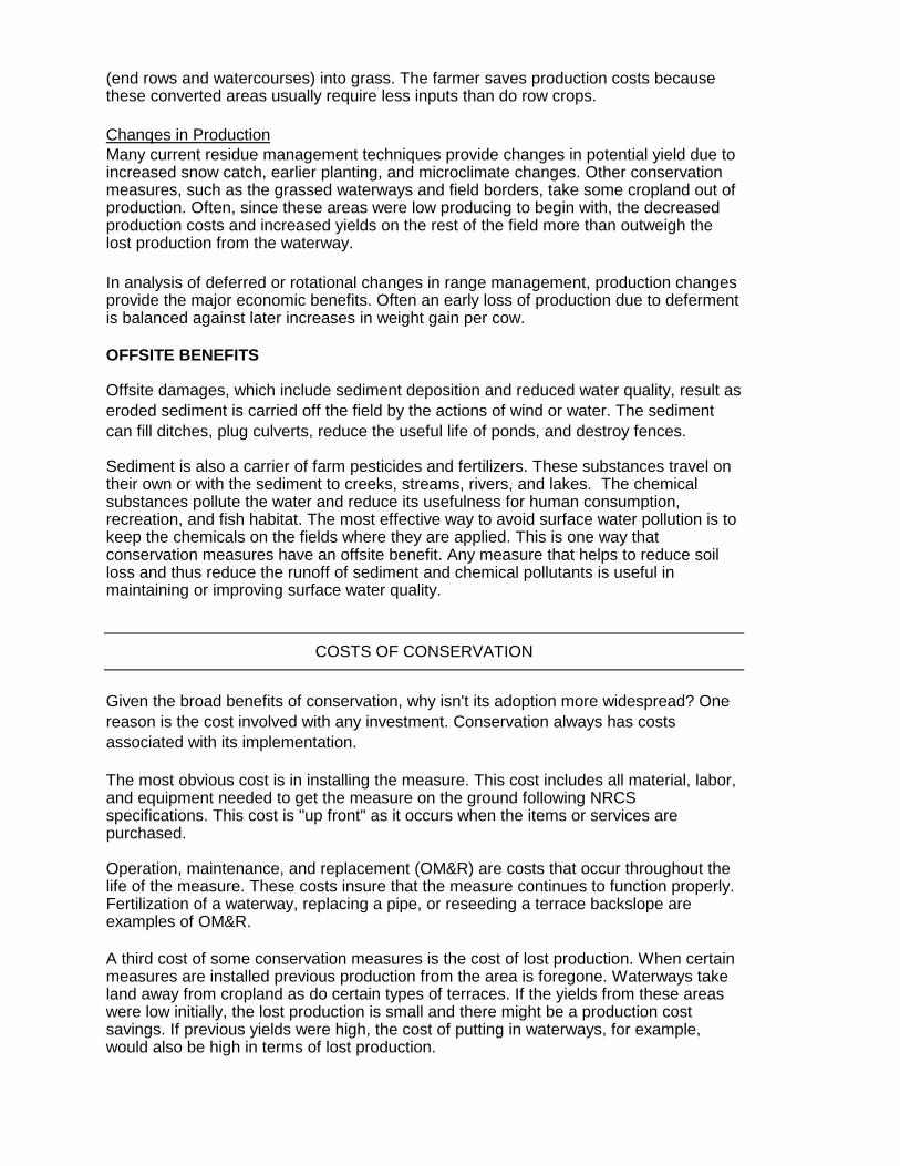
(end rows and watercourses) into grass. The farmer saves production costs because these converted areas usually require less inputs than do row crops.

Chanqes in Production Many current residue management techniques provide changes in potential yield due to increased snow catch, earlier planting, and microclimate changes. Other conservation measures, such as the grassed waterways and field borders, take some cropland out of production. Often, since these areas were low producing to begin with, the decreased production costs and increased yields on the rest of the field more than outweigh the lost production from the waterway.

In analysis of deferred or rotational changes in range management, production changes provide the major economic benefits. Often an early loss of production due to deferment is balanced against later increases in weight gain per cow.

OFFSITE BENEFITS

Offsite damages, which include sediment deposition and reduced water quality, result as eroded sediment is carried off the field by the actions of wind or water. The sediment can fill ditches, plug culverts, reduce the useful life of ponds, and destroy fences.

Sediment is also a carrier of farm pesticides and fertilizers. These substances travel on their own or with the sediment to creeks, streams, rivers, and lakes. The chemical substances pollute the water and reduce its usefulness for human consumption, recreation, and fish habitat. The most effective way to avoid surface water pollution is to keep the chemicals on the fields where they are applied. This is one way that conservation measures have an offsite benefit. Any measure that helps to reduce soil loss and thus reduce the runoff of sediment and chemical pollutants is useful in maintaining or improving surface water quality.

COSTS OF CONSERVATION

Given the broad benefits of conservation, why isn't its adoption more widespread? One reason is the cost involved with any investment. Conservation always has costs associated with its implementation.

The most obvious cost is in installing the measure. This cost includes all material, labor, and equipment needed to get the measure on the ground following NRCS specifications. This cost is "up front" as it occurs when the items or services are purchased.

Operation, maintenance, and replacement (OM&R) are costs that occur throughout the life of the measure. These costs insure that the measure continues to function properly. Fertilization of a waterway, replacing a pipe, or reseeding a terrace backslope are examples of OM&R.

A third cost of some conservation measures is the cost of lost production. When certain measures are installed previous production from the area is foregone. Waterways take land away from cropland as do certain types of terraces. If the yields from these areas were low initially, the lost production is small and there might be a production cost savings. If previous yields were high, the cost of putting in waterways, for example, would also be high in terms of lost production.

Another cost occurs with some tillage practices. It is possible that applications of fertilizers and chemicals must be increased in some solIs when switchlng to conservatlon tlllage or no-till. Increased production costs must be accounted for in these situations.

HOW THE TOTAL AGRICULTURAL ENVIRONMENT AFFECTS CONSERVATIONPURCHASES

Now that some benefits and costs of conservation have been discussed, how does the agricultural environment (interest rates, farm program, politics, etc.) affect a producer's decision to apply conservation? During times of prosperity, farmers can invest in long-term conservation. In fact, in years of high profit, farmers are searching for ways to reduce their tax burden. Under current tax laws, conservation is an intelligent investment for this purpose. In bad times, taxes are not a problem because profits are low. Since benefits from conservation sometimes take time to materialize while most costs are up front, lack of cash flow becomes a major problem for many farmers.

We need to be aware of a farmer's economic situation as we make our recommendations. Measures with high installation costs and benefits that take time to appear may be a good alternative from NRCS’s standpoint but not feasible for the producer. In times of economic stress, applying part of a system, although it may not completely solve the resource problem, is better than not applying any measures at all. At least the door remains open for the farmer when times get better to apply remaining practices of the resource management system and reap the full benefit of conservation.

ECONOMICS AND THE PLANNING PROCESS

The NRCS National Planning Procedures Manual (NPPH) describes planning as a flexible, continuing process of identifying problems and opportunities, determining objectives, inventorying resources, analyzing resource information, and developing and evaluating alternatives to help landusers make and carry out decisions toward management of their soil, water, and related resources.

To accomplish the goal of effective planning, NRCS uses a specific planning and implementation process consisting of nine elements in the delivery of assistance. This process is used in all instances where assistance is provided to decision makers whatever the expected outcome or scope of the planning effort, type of conservation treatments that are expected to be accomplished, and source of funding to be used for implementation.

The degree of detail used in the planning process will vary with the type, method, scope of assistance, complexity of the planning situation, and the recipient of assistance. Using the nine elements in the process in sequence creates a consistent method of providing assistance nationwide. The nine elements in planning and implementation are:

1. Identify the problem 2. Determine the objectives 3. Inventory the resource data 4. Analyze the resource data 5. Formulate alternative solutions 6. Evaluate alternative solutions

7. Client determines a course of action 8. Client implements the plan 9. Evaluation of the results of the plan

This process requires the use of interdisciplinary skills to achieve the highest quality of assistanc. Economics can and must play an important role in the plannlng process.

BASIC CONSIDERATIONS AND ECONOMIC PRINCIPLES

INTRODUCTION

This chapter deals with defining and illustrating economic principles and procedures that can contribute to efficient conservation planning and effective decision making. Emphasis is placed on the identification of basic effects for purposes of comparison and selection. A secondary purpose is to define levels of sophistication in analysis and incorporate consideration of factors that significantly impact the relative attractiveness of alternatives to decision makers. Contents of this chapter are based on the belief that economics is inseparable from planning and that the role of economics, like planning, is ultimately aimed at providing responsible information that allows landusers to make informed decisions about: 1) what to do, and 2) how to do it.

FUTURE CONDITIONS, WITH AND WITHOUT CONSERVATION

The need for conservation planning is based on the premise that some physical situation, such as erosion or yield level, is currently or is expected to be at a condition that is undesirable or unacceptable. The effects of present and future situations without taking any action should be compared to those expected with implementation of an action. This difference between the with and without action conditions is the measure of change.

Estimating effects into the future is important. Effects should neither be overstated nor understated. Reference must be made to time. Consider an example where current mismanagement of grazing resources is causing a decline in range condition. Without

Future AUM Production

150

100

50

0 0 5 10 15 20 25

Years

Present Condition Future, No Treatment Future, with Treatment

change in management continued overgrazing will cause range production to decline from 100 animal unit months (AUMs) today to 90 AUMs in 25 years. With adoption of a planned grazing system, range condition will tend to improve. Potential production will improve from the 100 AUM today to 135 AUMs in 25 years. The following graph illustrates the differences.

Estimates of future conditions with and without treatment are commonly made by using an inventory of current conditions as a beginning point; then, historical trends are projected while considering current relationships and foreseeable developments (the upper and lower lines above). Projections should reflect the views of the decision-makers, research, and other published data such as soil surveys. Most important, expectations of future conditions with and without treatment must be tempered by local judgment.

The economic benefit in the above example would be the actual area between the lower and upper lines; between 90 AUMs and 135 AUMs at 25 years, not between the original 100 AUMs and 135 AUMs.

DECISIONMAKING

Effective conservation planning must have involvement of both the planner and decision-maker. The decision-maker must identify the important physical and/or economic factors that should be examined for change between expected future with and without conditions. In addition, the decision-maker must also identify the relevant time horizon.

Ultimately, the decision-maker must also place relative value on the gains and losses to find their individual choice.

Balancing gains against losses in decision making often involves comparing factors that are not compatible in kind, place, or time. Some effects may have a common denominator such as a market price while others do not. Wildlife availability and landscape appearance are two examples where commonly held absolute values do not exist.

LEVELS OF DETAIL

Assistance is normally provided up to the point where landusers can comfortably make an informed decision leading to conservation actions. The kind and amount of information will be different for every individual and every situation.

The simplest level of evaluation may consist only of identifying the most obvious physical impacts stemming from the problem and estimating the costs of the conservation practices that address these problems. A vast majority of the questions posed by owner/operators can be answered with this approach.

An intermediate level of evaluation could be used where more specific questions on the resource problems require more detailed answers. The chapter on Evaluation Techniques will discuss these options at length.

Where an individual cooperator requests an advanced level of analysis, field personnel involved may need to request direct assistance from the state economist.

PERIOD OF ANALYSIS OR PLANNING HORIZON

Two analytical concerns in decision making are figuring out the length of time over which effects are considered and converting these effects to a common time basis. The length of time over which effects are considered is called the period of analysis or planning horizon. The decision-maker is responsible for identifying the planning horizon. General factors affecting the decision maker in the determination of planning horizons are age of the cooperator and intergeneration transfer (whether the children will farm), etc. Economic factors which decide the period of analysis include physical deterioration of capital investment (i.e., farm equipment, conservation practices, etc.) and obsolescence due to improvements in technology. The planning horizon may exceed the economic life of the alternative. If the planning horizon is shorter than the economic life of the alternative, take care to account for the benefits that accrue beyond the period analyzed and any costs that may be recoverable at the end of the period.

LEAST COST ALTERNATIVE

From an economic viewpoint, any conservation practice selected for installation should satisfy the requirement that it not be more costly than any reasonable alternative means of accomplishing the same specified objective. Comparison of costs for all alternatives considered is essential and should include the estimate of operation, maintenance, and replacement expenditures besides the annual installation costs. Any costs occurring in the future need to be identified and converted to a common time base.

MAXIMIZATION OF NET INCOME (PROFIT)

The optimum scale of economic output from application of conservation practices is the point at which net income is at a maximum. This occurs when the income added by the last increment of input is equal to the cost of adding that increment. The increments to be considered are those smallest units in which there is a practical choice as to inclusion or omission from the proposed package of conservation practices. This process is best described as equating the marginal returns (income) and the marginal costs (expense).

TIME AND MONEY

INTRODUCTION

Modern American agriculture is a complex business. As farms get bigger and investments higher, more knowledge is required to figure out costs and returns and analyze alternatives. An understanding and proper use of interest and annuities is necessary in analyzing and comparing the many investments and alternatives available.

Money can be used either to satisfy immediate wants or be invested in capital goods with present or future productive capacity. Demand, time, and risk determine rates of interest (payment for the use of money). If funds are borrowed, the rate must be applicable to the type and length of loan needed. If funds are not borrowed, the rate used will depend on the desire for and opportunity of obtaining returns from using the funds in other productive uses (opportunity cost).

The intent of this chapter is to provide a basic understanding of interest and annuities and how they can be used to compare and analyze investments and alternatives. This

chapter will also use the financial functions in computer spreadsheets, and small financial calculators. An older method for the noncomputer literate uses interest and annuity factor tables in Chapter 4. Contact your state resource conservationist or economist for tables of other interest rates needed. This chapter also gives formulas and examples for calculating the interest factors. To help put things in proper perspective, it is sometimes helpful to draw a sketch or diagram of the situation being analyzed.

TIME VALUE OF MONEY AND OPPORTUNITY COST

Money can be invested and used to make more money over time. Thus, the dollar received today could be put into a bank or invested elsewhere. It would be worth more than one dollar a year from now. This concept, the time value of money, is dealt with in home and business finance every day. For example, landusers may make decisions about purchasing one piece of equipment versus another or no purchase at all, based on the use of money over time.

The time value of money can be thought of in two ways. First, if the landuser borrows money for a purchase, the time value of money is the interest paid on the loan. If the landuser uses his own money for a conservation measure, the time value of money would be the return he gave up from another investment (savings account, certificates of deposit (CD), IRA, etc.). He has an “opportunity cost." The interest he could have received from a CD is now a lost opportunity because he used the funds for conservation.

When a landuser considers purchasing conservation, the idea of time value of money applies. There is a cost above and beyond the purchase of the conservation measure. If the landuser borrows to pay for the measure, that additional cost will be equal to the interest he must pay on the loan. If he uses his own money, the additional cost is equal to the return that money would have earned in another investment.

ONE-TIME VALUES, ANNUAL FLOWS (ANNUITIES) AND LAGS

The benefits and costs of conservation do not necessarily occur simultaneously. Certain costs and benefits may occur at one point in time while others occur over several years. Some occur today while others occur in the future.

Those values that occur at one point in time are called one-time values. Installation costs are an example of a value that occurs at one time. Values that occur over time are called annual flows or annuities. Annuities can be generalized into constant, decreasing, and increasing over time, depending on their characteristics. Many benefits from conservation fall into the annuity category.

A one-time value can occur today or at some point in the future. If it occurs at some point in the future it is said to be "lagged" or delayed. The replacement cost of a practice is a good example of a lagged one-time value. Annuities too can be lagged. If benefits from a terrace do not start until one year after installation, then those benefits are said to be lagged one year. The benefits from deferred grazing following range seeding are another common occurrence of a lagged annuity.

Table 1 illustrates examples of one-time values, annual flows, and lags.

Table 1

ONE-TIME VALUE ANNUAL FLOW – AVERAGE LAGGED VALUES ANNUAL VALUES

Installation Cost Conservation Benefits Replacement Cost

Replacement Cost

Average Returns

Average Costs

Any value not starting this year

O&M Costs (Average)

AVERAGE ANNUAL VALUES

To compare benefits and costs, they must be considered in the same period; otherwise we are comparing apples and oranges. A standard term has been developed called average annual values. Average annual values are nonlagged annual flows. In Table 1, the middle column gives four examples.

One significance of average annual values is that most businesses, including farming, have accounting systems that are based on average annual values. Therefore, the costs and benefits of conservation, once converted to average annual values, can be added to the costs and returns of the farm business.

Average annual and amortization values are often confused. The amortization value is the value that is required to payoff a loan or investment with interest in constant amounts during a period. Amortizing a $50,000 mortgage on a house at 9 percent over 30 years calculates out to a $402 monthly mortgage payment. However, the average monthly cost of owning that house would also include allowances for the downpayment, taxes, insurance, and the cost of a new roof in 10 years.

TOOLS FOR INTEREST CALCULATIONS

There are four types of useful tools for converting benefits and costs of conservation into average annual values that we will consider. All these tools require knowledge of four of the five variables to solve the missing variable. In problems that need only three variables, one variable is assumed to be zero. These five variables are:

N = Number of periods, whether years for most SCS problems or months for your home mortgage payment.

I or r = Interest rate for each period. Make sure when doing monthly interest, to enter the interest per month, not the interest per year.

PV = Present Value = Value of the money today.

FV = Future Value = How much money left at the end of the analysis.

PMT = Payment made or income received per period.

1. A calculator with financial functions should be used. All NRCS employees are encouraged to have financial functions on any new calculators. They are the

handiest and the fastest tool for financial calculations. All business calculators will take any four of the following five variables and solve for the missing variable:

For example, to buy a tractor for $50,000 today, borrowing all money at 10 percent in a 5-year loan, what would your annual loan payment be?

PV = $50,000 Initial loan N = 5 years FV = 0 (The loan will be paid off after five years). I = 10%

Now press PMT to calculate the annual payment of $13,190. To figure the average annual cost, assume that the tractor sells for $35,000 after 5 years. Change FV to $35,000 and press PMT to get $7,457 annual cost.

2. Computer spreadsheets; such as EXCEL or LOTUS 123 are good tools for economic analysis. All spreadsheets have the following financial functions. Note how each of these functions needs three of the above variables, assumes the fourth equals zero, and solves for the fifth number.

FV returns the future value of a series of equal payments (pmt) earning interest for a number of terms (n), if the payments are invested at an interest rate (r).

PV returns the present value of a series of equal payments (pmt) that are received for a number of terms (n), if the payments are invested at an interest rate (r).

PMT returns the equal payment on a loan of principal (PV) with interest (r) and payment period (n).

RATE returns the interest rate that will enable an investment of present value (PV), to grow into a future value (FV), over terms (n).

TERM returns the number of payment periods needed to reach a future value (FV) given payments (PMT) and an interest rate (r).

3. Amortization key (discussed later in this chapter)

4. Using Interest and Annuity (I&A) Tables. The conversion of costs and benefits of conservation to average annual values without the help of I&A tables would involve the use of many difficult formulas and calculations. These tables were constructed to simplify the process by presenting coefficients developed from the formulas, thus providing much simpler calculations. Formulas and examples are provided for those who would like to use them.

Interest and annuity tables are available for a wide range of interest rates. An interest rate of 10 percent has been used in the following examples. The table that NRCS in South Dakota uses has eight columns: (1) number of years hence, (2) compounded value of one, (3) present value of one, (4) amortization, (5) present value of an annuity of one per year, (6) amount of an annuity of one per year, (7) present value of an increasing annuity, and (8) present value of a decreasing annuity. All these items are discussed in detail below.

"Number of years hence" is the number of years in which calculations are considered. This is n in the spreadsheets and financial calculators. Several factors may influence this determination: (1) the period may last a year or indefinitely (perpetuity), (2) the measures may have a short or long useful life, or (3) an individual may want to recover his/her costs in a certain time period.

Two items that are discussed in detail but are not found directly in the tables are: (1)simple interest and (2) sinking fund. These will be illustrated and procedures shown to arrive at the correct factor. Note that compounded interest has been added to the tables. This assumes interest is compounded once per year, not monthly as in home mortgages, or daily as in some bank accounts.

SIMPLE AND COMPOUND INTEREST

Interest is the earning power of money, or the rent of the use of money. Interest is usually expressed as an annual percentage rate (APR) and may be either simple interest or compound interest.

1. Simple Interest: Money paid or received for the use of money generally calculated over a base period of one year at a set interest rate.

Formula: i = (p) (r) (n), where i = interest, p = principal, r = interest rate and n = number of periods (years).

Example: $7,000 is borrowed at 10 percent interest (APR) for 1 year. How much money will be needed to payoff this loan when it is due?

i = 7,000 x .10 x 1 = $700 of interest will be due $7,000 of principal will be due $7,700 to payoff loan

Example: $3,000 is put into a savings account for 6 months at 10 percent interest (APR), how much interest will be earned?

I = 3,000 x .10 x .5 = $150 will be earned.

2. Compound Interest: Interest that is earned for one period and immediately added to the principal, thus, resulting in a larger principal on which interest is computed for the following period.

Formula: (1 + i)n, where n = number of periods, i = periodic rate of interest, and one represents $1 since the formula results in a factor that is multiplied by the principal dollar amount.

If the interest rate is 10 percent (APR) compounded quarterly for 5 years, then i = .10/4 (four payments in a year) or .025; n = 5 x 4 (4 payments in a year) or 20. One factor to be multiplied by the principal amount is (1 + .025)2 = 1.63862.

Example: $2,500 is put into a savings account paying 10 percent interest compounded ANNUALLY. How much will be in the account of this depositor at the end of seven years?

(1 + .10)7 = 1.9487171; 1.9487171 x $2,500 = $4,871.79

i

$2,750 $3,025

$3,660

$4,429

$4,872

$-

$1,000

$2,000

$3,000

$4,000

$5,000

$6,000

0 1 2 3 4 5 6 7

Compounding Example $2,500 Sav ngs over 7 years at 10%

$2,500

$3,328

$4,026

Years

For comparative purposes, compounding gives these results:

Compounded SEMIANNUALLY (1 + .05)14 * $2,500 = $4,949.83

Compounded QUARTERLY (1 + .025)28 * $2,500 = $4,991.24

Compounded MONTHLY (1 + .0083333)84 * $2,500 = $5,019.79

Compounded DAILY (1 + .0002740)2555 * $2,500 = $5,034.25

Compound interest factors are shown in the tables. Also, the same answer can be obtained by dividing one by the appropriate "present" value of one dollar factor since the present value of one is the reciprocal of the compound interest factor. Since these are "annual" tables, this method will work only if compounding on an annual basis.

Example: Using the preceding problem, what will $2,500.00 grow to in 7 years at 10 percent interest compounded annually. 1/.51316 (from the interest tables, present value of 1, 7 years hence at 10 percent) = 1.948710 the same factor was obtained by using the formula 1.948710 x $2,500.00 = $4,871.78.

PRESENT VALUE OF 1

The present value of one is the amount that must be invested now at compound interest to have a value of one in a given length of time, or what $1 due in the future is worth today. It is also known as the present worth of one or the discount factor.

Formula: 1 (The "present value of 1" factor is the reciprocal of the "compound interest"

n (1 + i) factor.)

Example: $4,000 will be needed 5 years from now. How much would need to be invested today at 10 percent interest .compounded annually to reach that goal?

1 1 (1 + 0.10) 5 = 1.61051 = .62092

This amount would need to be invested now at 10 percent interest compounded annually to be worth $4,000.00 in 5 years 0.62092 x $4,000.00 = $2,483.68.

The factor can also be found in the 10 percent interest table in the "present value of 1" column for five years hence.

Example: What is the discounted value of $10,000 at 10 percent interest for 25 years?

From the table 0.09230 X $10,000 = $923. Looking at it another way, if you invested $923.00 at 10 percent interest compounded annually and left it alone for 25 years, you will have $10,000 at the end of the 25 years (the power of compounding). Ten thousand dollars to be received in 25 years is worth $923 today.

AMORTIZATION

Amortization is also called the partial payment or capital recovery factor. It is the extinguishing of a financial obligation in equal installments over time. The amortization factor will find what annual payment must be made to payoff the principal and interest over a given number of years (average annual cost).

nFormula: i(1 + i) i (1 + i)n-1 or 1- 1

n (1 + i)

Example: A farmer borrows $7,000 to install a resource management system. The interest rate is 10 percent and the repayment schedule is set up for 10 years. What is his average annual cost, the amount he must pay each year, for 10 years to payoff the loan and interest?

.10 1 - 1 = .10 = .10 = .16275 (1 + .10)10 1 - .38554 .61446

.16275 x $7,000 = $1,139.25 this amount must be paid each year for 10 years to payoff the $7,000 loan and interest. A total of $11,392.50 will have been paid to close out this loan ($7,000 of principal and $4,392.50 of interest).

The following table displays what occurs each year during the 10-year period.

Year Loan

Annual Balance

Amount of Payment

Principal Interest Remaining

1 2 3 4 5 6 7 8 9

10 $0 l - -

i ii

i=

Amortization Problem

0 $0

0 1 2 3 4 5 6 7 8 9

Loan

$7,000.00 $1,139.25 $439.25 $700.00 $6,560.75 $6,560.75 $1,139.25 $483.17 $656.08 $6,077.58 $6,077.58 $1,139.25 $531.49 $607.76 $5,546.09 $5,546.09 $1,139.25 $584.64 $554.61 $4,961.45 $4,961.45 $1,139.25 $643.11 $496.14 $4,318.34 $4,318.34 $1,139.25 $707.42 $431.83 $3,610.92 $3,610.92 $1,139.25 $778.16 $361.09 $2,832.76 $2,832.76 $1,139.25 $855.97 $283.28 $1,976.79 $1,976.79 $1,139.25 $941.57 $197.68 $1,035.22 $1,035.22 $1,139.25 $1,035.73 $103.52

Tota $11,392.50 $7,000.00 $4,392.50

The factor can also be found in the 10 percent interest table in the "amortization" column for 10 years hence.

NOTE: The amort zat on factor is the reciprocal of the "present value of an annuity of one per year" factor. This same answer can be obtained by div ding by the "present value of an annuity of one per year" factor. Using the above problem, the solut on is as follows:

$7,000 / 6.14457 $1,139.22

$7,000 loan paid off at 10% over 10 years

$1,139 $1,139 $1,139 $1,139 $1,139 $1,139 $1,139 $1,139 $1,139 $1,139

$7,000

$1,000

$2,000

$3,000

$4,000

$5,000

$6,000

$7,000

$8,000

10

Years

Loan Payment

AMORTIZATION KEY

Many plant science or botany courses, a tool called a "Key" is used to identify plant species by answering a series of questions. This "keying out" process is useful because it allows nonexperts to identify species of plants that are unknown to them. By

answering a series of questions, the amortization key serves as a guide for using the interest and annuity tables to convert benefits and costs of conservation to average annual values. The first question on the key is whether the value is an annuity, like benefits from a terrace that flow over time, or if it is a one time value like terrace installation costs. If it happens to be a one-time value, move down the key to the question, "Is it lagged?" A value that will be realized some time in the future is considered lagged because there is a lag period between now and the time the value takes place. Assuming the value is not lagged, then the only adjustment needed is to amortize the value over the life of the project or evaluation period.

This is accomplished by multiplying the amortization factor found in the tables times the one time value. This results in an average annual value. Had it been lagged, the one time value would first have to be multiplied by the "present value of one" factor for the lag period, then multiplied by the amortization factor to convert to average annual.

To convert an annuity to an average annual value, it is important to decide if the annuity is constant, increasing, or decreasing. If the annuity is a constant flow of value, then it should be multiplied by the "present value of a constant annuity" factor for the period (years) of the annuity. This factor is found in the I&A tables under the column called "present value of an annuity of one per year."

The result of this multiplication would then be multiplied by the amortization factor if the annuity was not lagged. If the annuity period was lagged, it would be multiplied by the "present value of one" factor for the lag period before being amortized.

For increasing or decreasing annuities, recall that the value used to multiply all the factors by, is the yearly average increase or decrease. For example, for an increasing annuity that begins at 0 and rises to $500 after 5 years, the yearly average increase would be 500 divided by 5, or 100. That value would be taken times the "present value of an increasing annuity" factor five years. Locate the factor in the 5-year row under the present value of an increasing annuity column and take it times 100. If the annuity is lagged, that answer is multiplied by the "present value of one" factor over the lag period or just amortized if the annuity begins in the first year. The same steps would be taken for a decreasing annuity using the appropriate factors.

To summarize, the first step in the process is to convert any annuity into a one-time value. Then we adjust for any lags that are present. Finally, we amortize. Thus, we have three basic steps in our process:

1. Convert annuities to one-time values

2. Adjust for lags

3. Amortize

Note: Not all steps are used each time. The key guides you through the proper process. For example, if a one-time value is considered, the key moves you past step one. If the annuity or one-time value is not lagged, the key moves you past step two. Remember, this process is necessary to convert benefits and costs of conservation into values that can easily be incorporated into a farmer's records and decision-making system.

AMORTIZATION KEY

Annuity ( )

over time

Type of Annuity

Constant Increasing

PV of constant annuity over life of annuity

PV of increasover life of an

s

PV

Amo

AVERAGE A

Type of Value

1 Ti

STEP 1

me Value

Decreasing

ing annuity nuity

PV of decreasing annuity over life of annuity

Is it lagged?

STEP 2

Ye

of 1 over lag period

rtize over life of project

NNUAL VALUE

No

STEP 3

PRESENT VALUE OF AN ANNUITY OF ONE PER YEAR

Present value of an annuity of one per year is also called a constant annuity, present worth of an annuity, or capitalization factor.

This factor represents the present value or worth of a series of equal payments or deposits over a period. It tells us what an annual deposit of $1 is worth today. If a fixed sum is to be deposited or earned annually for "n" years, this factor will find the present worth of those deposits or earnings.

l ( n-1

i (l n Formu a: 1 + I)

+ i)

Example: You want to provide someone with $1,200 a year for 10 years. The interest rate is 10 percent. How much do you need to deposit to produce $1,200 a year for 10 years?

) (1 + .10 10-1 = (1.10)10-1 = 1.59374 = 6.14457 .10(1 + .10)10 .10 (2.59374) .259374 6.14457 x $1,200.00 = $7,373.48 this amount must be deposited now to produce an annuity of $1,200 for 10 years. A total of $12,000 will have been received from this one­time deposit of $7,373.48. The interest amounts to $4,626.52.

Present Value of an Annuity $1,139 Annual Payment over 10 years

$8,000

$7,000 $7,000

$6,000

$5,000

$4,000

$3,000

$1,000

$2,000 $1,139 $1,139 $1,139 $1,139 $1,139 $1,139 $1,139 $1,139 $1,139 $1,139

$0 0 1 2 3 4 5 6

Years 7 8 9 10

lAnnual Income Present Va ue

The factor can also be found in the 10 percent interest table in the "present value of an annuity of one per year" column for 10 years hence.

i i iNOTE: the factor is the reciprocal of the “amortization: factor. Therefore, the same

answer can be obtained by div ding by the amort zat on factor

AMOUNT OF ANNUITY OF ONE PER YEAR

The amount of an annuity of one per year is the amount that an investment of $1 per year will accumulate in a certain period at compound interest.

l )n -1 i

Formu a: (1 + i

Example: $2,000 per year will be invested in an individual retirement account (IRA) for 30 years paying 10 percent interest compounded annually. What will be the value of this account at the end of the 30 years?

.10 (1 + .10) 30 –1 =

.10 16.449402 = 164.49402

164.49402 x $2,000 = $328,988.04; value of the IRA account at the end of 30 years.

Future Value of an Annuity $1,139 Annual Payment over 10 Years

$8,000

$7,000

$6,000

$5,000

$4,000

$3,000

$2,000

$1,000

$­1 2 3 4 5 6 7 8 9 10 11

$1,139 $1,139 $1,139 $1,139 $1,139 $1,139 $1,139 $1,139 $1,139 $1,139

$7,000

Years

lAnnual Income Total Future Va ue

The factor can also be found in the 10 percent interest table in the “amount of an annuity of 1 per year” column for 30 years hence.

SINKING FUND

The sinking fund factor is used to find what size annual deposit will be required to accumulate a certain amount of money in a certain number of years at compound interest.

Formula: i (1 + i)n - 1

Example: $6,300 will be needed in 4 years. What amount will need to be deposited each year at 10 percent compound interest to reach this goal?

.10 = .10 = .21547 (1 + .10)4 -1 .4641

0.21547 x $6,300 = $1,357.46; this amount must be deposited annually for 4 years at 10 percent interest, compounded annually to accumulate the $6,300.

Sinking Fund Example $1,139 saved for 10 years at 10% to reach $18,156 College Fund

$-

$1,139 $1,139 $1,139 $1,139 $1,139 $1,139 $1,139 $1,139 $1,139 $1,139

$18,156

$2,000

$4,000

$6,000

$8,000

$10,000

$12,000

$14,000

$16,000

$18,000

$20,000

1 2 3 4 5 6 7 8 9 10 11 Years

l ll iTota Co ege Fund Annual Savngs

i

i i i

NOTE: The sinking fund factor is not shown in the tables but the same answer can be obtained by div ding by the appropriate "amount of an annuity of one per year" factor. This is because the amount of an annuity of one per year factor is the reciprocal of the sinking fund factor.

NOTE: The sinking fund factor is also equal to the amort zat on factor m nus the interest rate.

.31547 - .10 = .21547; .21547 x $6,300 = $1,357.46 )

PRESENT VALUE OF AN INCREASING ANNUITY

The present value of an increasing annuity is a measure of present value of an annuity that is not constant but increases uniformly over a period. When using this factor, it is important to note that the value of $1 (which is multiplied by the factor) is the annual rate of increase and not the total increase during the period.

l )n (I)2

Formu a: (1 + i n+1 – (1 + i) –n(i) (1 + I)

Example: A farmer renovates a pasture and estimates that it will reach full production in four years. The improvement will increase uniformly over the 4-year period and at full production will improve net income $20 per year per acre. Using an interest rate of 10 percent, what is the present value of this increasing annuity?

(1 + .10)5 – ( 1 + .10) –4 (.10) = 1.61051 - 1.1 - .4 = .11051 = 7.54798

.10)2 (1 + .10)4 ( 1.46410 x .01 .014641

We now need to find the annual rate of increase. The annual rate of increase is $20/4 or $5.

lPresent Va ue of Income Stream This Year's Income Past years Income + 10% Interest Future Value of an Increasing Annuity

Adding an extra $5 per year at 10%

$60.00

$50.00

$40.00

$30.00

$20.00

$10.00

$­

$37.74

$5.00 $10.00

$15.00 $20.00

$5.50

$17.05

$35.26

0 1 2 3 4

Years

This is to say that the annuity is not constant each year but increase income of $5 the first year, $10 the second year, $15 the third, and $20 the fourth year (increases uniformly at $5 per year). The present value of this increasing annuity or income stream is then 7.54798 .x $5 or $37.74. This also means that if $37.74 was deposited in an account paying 10 percent interest

compounded annually, $5 could be withdrawn after year I, $10 after year 2, $15 after year 3, and $20 after year 4, leaving a balance of $0.

The factor can also be found in the 10 percent interest tables in the "present value of an increasing annuity" column for 4 years hence.

PRESENT VALUE OF A DECREASING ANNUITY

The present value of a decreasing annuity factor is used to find how much something is presently worth that will provide an annuity that decreases uniformly each year. Again, it is important to note that the value of $1 (which is multiplied by the factor) is the annual rate of decrease and not the total decrease during the period.

1 nFormula: n(i) – 1 + (1 + i)

(i)2

Example: A gravel pit is producing $28,000 income annually. Due to a decreasing supply that is costlier to remove, income will drop at a steady rate until it equals zero in seven years. At 10 percent interest, what is the present value of the gravel?

1 1 7(.10) – 1 + (1 +.10)7 = -0.3 + 1.17 = -.03 + 0.513158 = .0213158 = 21.31581 (10)2 .01 .01 .01

Future Value of a Decreasing Annuity Declining Income from Gravel Pit

$200,000

$180,000

$160,000

$140,000

$120,000

$100,000

$80,000

$60,000

$40,000

$20,000

$­0 1 2 3 4 5 6

$-$28,000 $24,000 $20,000 $16,000 $12,000 $8,000 $4,000

$30,800 $60,280

$88,308 $114,739

$139,413 $162,154

$182,769

Years

This Years Income Past Years Income + 10%

7

We now need to find the annual rate of decrease. The annual rate of decrease is $28,000/7 or $4,000. The annuity is not constant each year. He will receive income of $28,000 the first year, $24,000 the second, $20,000 the third, etc., until the supply runs out on the 7th year and becomes $0.

The present value of this decreasing annuity or income stream is then 21.31581 x $4,000 or $85,263.24; this is the amount that would need to be deposited now to produce the identified decreasing annuity.

The factor can also be found in the 10 percent interest table in the "present value of a decreasing annuity" column for 7 years hence.

RULE OF 72

The rule of 72 states that 72 divided by the interest rate received will result in the number of years it will take to double your money at compound interest.

Example: At 8 percent compound interest how long will it take to double an investment of $150?

72.8 = 9 years to double your money ($300)

PROOF: PV of one, nine years hence, at 8% = .50025 (from I & A Tables). .50025 x $300 = $150

OR

Dividing 72 by the number of years you want to double your money in will result in the interest rate needed to double the investment.

EXAMPLE: At compound interest, what interest rate would you need to receive to double $150 in nine years?

72 / 9 = 8% return needed to double your investment in nine years.

PROOF: $150 / .50025 = $300

NOTE: Compound interest factors are not shown by column heading in the I&A tables. However, the answer can be obtained by dividing by the appropriate "present value of one" factor (0.50025) since the present value of one factor is the reciprocal of the compound interest factor. Since these are "annual" tables, this method will work only if compounding on an annual basis.

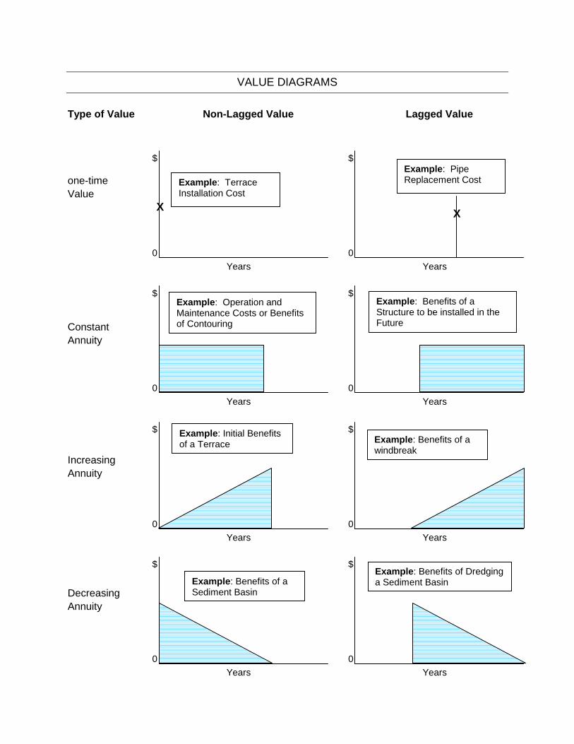
VALUE DIAGRAMS

Type of Value Non-Lagged Value Lagged Value

iValue

0

$

0

$

:

X

: Pipe

X

one-t me Example Terrace Installation Cost

ExampleReplacement Cost

Years Years

0

$

0

$ : :

Constant Annuity

Example Operation and Maintenance Costs or Benefits of Contouring

Example Benefits of a Structure to be installed in the Future

Years Years

0

$

0

$

wiIncreasing Annuity

Example: Initial Benefits of a Terrace Example: Benefits of a

ndbreak

Years Years

$

Decreasing Annuity

0 Years Years

0

$

in inExample: Benefits of a

Sediment Bas

Example: Benefits of Dredging a Sediment Bas

INTEREST RATE SELECTION ADVICE

The biggest single factor in any long-term economic calculation is the selection of which interest rate to use. The interest rate to be used should correspond to an opportunity cost equal to the best current investment available, plus any added risk charge, minus expected inflation in the price of the product.

Here is an example installing a $10,000 well to better utilize rangeland. Assume that this will create an additional $1,000 of income per year over the next 25 years. The following shows the cash flow, net return, and benefit/cost ratio at various interest rates. To simplify the examples no risk premium is included.

Rancher A has the $10,000 sitting in a 6 percent CD. He figures that cattle prices will increase over time by four percent annually. He calculates his opportunity cost as six percent interest minus the four percent expected increase in cattle prices for a net two percent opportunity cost.

Rancher B has the $10,000 sitting in a 7 percent CD. However, he does not assume any increase in the price of cattle nor increased production efficiency over the next 25 years. He uses the seven percent interest rate.

Rancher C will borrow the money on a 10 percent loan. He balances the risk premium against probable long-term increases in cattle prices.

Rancher D really wants to develop the well. However, he is mortgaged to the hilt. He borrows the $10,000 on his credit cards at 20 percent.

Finally, we will calculate the net internal rate of return, that interest rate at which the investment will break even. This calculation can easily be made only with a computer. LOTUS 1-2-3 and EXCEL, GRAZING LAND APPLICATION (GLA), and other NRCS programs will make this calculation.

The following example was produced in a few minutes using EXCEL. The formula used for each row is included in the rightmost column. Note that the Net Internal Rate of Return is only 8.78 percent for this example, despite delivering $25,000 of income for a $10,000 investment. That is a 2.5:1 B/C ratio without considering interest; 1.95:1 B/C with a low 2 percent interest rate; but the investment does not even break even at a 10 percent interest rate.

Water Development Example

Cash Present Value at: Year Income 2% 7% 10% 20%

0 ($10,000) Investment 1 $1,000 $ 980 $ 935 $ 909 $ 833 2 $1,000 $ 961 $ 873 $ 826 $ 694 3 $1,000 $ 942 $ 816 $ 751 $ 579 4 $1,000 $ 924 $ 763 $ 683 $ 482 5 $1,000 $ 906 $ 713 $ 621 $ 402 6 $1,000 $ 888 $ 666 $ 564 $ 335 7 $1,000 $ 871 $ 623 $ 513 $ 279 8 $1,000 $ 853 $ 582 $ 467 $ 233 9 $1,000 $ 837 $ 544 $ 424 $ 194 10 $1,000 $ 820 $ 508 $ 386 $ 162 11 $1,000 $ 804 $ 475 $ 350 $ 135 12 $1,000 $ 788 $ 444 $ 319 $ 112 13 $1,000 $ 773 $ 415 $ 290 $ 93 14 $1,000 $ 758 $ 388 $ 263 $ 78 15 $1,000 $ 743 $ 362 $ 239 $ 65 16 $1,000 $ 728 $ 339 $ 218 $ 54 17 $1,000 $ 714 $ 317 $ 198 $ 45 18 $1,000 $ 700 $ 296 $ 180 $ 38 19 $1,000 $ 686 $ 277 $ 164 $ 31 20 $1,000 $ 673 $ 258 $ 149 $ 26 21 $1,000 $ 660 $ 242 $ 135 $ 22 22 $1,000 $ 647 $ 226 $ 123 $ 18 23 $1,000 $ 634 $ 211 $ 112 $ 15 24 $1,000 $ 622 $ 197 $ 102 $ 13 25 $1,000 $ 610 $ 184 $ 92 $ 10

Sum of PV $25,000 $19,522 $11,654 $9,078 $4,948

Cost $10,000 $10,000 $10,000 $10,000 $10,000

Net Return $15,000 $9,522 $1,654 ($922) ($5,052)

Benefit/Cost 2.5 1.9522 1.1654 0.9078 0.4948 Ratio

Net Internal rate of Return: 8.78%

CONCEPT OF REAL INTEREST RATES

In the 1920's, an economist named Irving Fisher tried to prove that there was no connection between interest rates and the rate of inflation. However, he found that statistically there was a direct relationship. The prime lending rate over a century of data was close to a base rate of two to three percent plus the expected inflation rate. The expected inflation rate is the rate of inflation that lenders expect to occur over the life of the loan based on their recent history of inflation. The Real Interest Rate is the normal interest rate minus the expected inflation rate.

The logic of this is simple. When you buy a 10-year bond or CD you expect that money 10 years from now to be worth less due to inflation. Since 1940 this country has had almost continual inflation. Since 1982 inflation has stayed between 3 and 6 percent annually. The Federal Reserve Board in the 1980's regulated the money supply to achieve a stable 4 percent inflation rate. If you lend out money for 10 years, you need a 4 percent interest rate just to maintain purchasing power. The real interest rate would be any additional interest received over the four percent expected inflation rate.

For most of the last 200 years, real interest rates have averaged about 3 percent. Additional percentages were added for risk premiums and bank profits for farm, home, and commercial loans. Four percent expected inflation plus three percent real interest equals seven percent; which is about the Treasury bond rate today.

A form of the real interest rate should be used for most long-term investments today if the price of the product is expected to grow over time. Overall construction costs have increased roughly with the inflation rate. Thus house prices, based on increasing replacement costs, should eventually increase in stable or growing communities. The value of recreation trends to increase at a greater rate than the CPl. Agricultural input prices generally go up with inflation. A real interest rate could be used with most investments that reduce input costs.

Grain and livestock prices are highly variable to supply and demand fluctuations and have little relation to general inflation. However, both grain and livestock production have continual efficiency gains that economically have a similar function. Corn yields in South Dakota were over 54 bushels an acre for only 1 year before 1977. They have not been below 54 bushels an acre since then. Soybean and wheat yields have similar patterns. Hog, beef, and dairy production are also continually increasing in productivity, whether on a per animal or feed efficiency basis. From an economic perspective, an increase in general efficiency has the same effect as an increase in prices over the long-term. These efficiency gains are the main reason that farmers can continue to sell corn for half parity price and still stay in business.

FEDERAL WATER AND RELATED LAND RESOURCES DISCOUNT RATE

NRCS and other federal agencies following Economic and Environmental Principles and Guidelines for Water and Related Land Resources Implementation Studies must use the current federal project discount rate for watershed planning. This rate is mandated for PL566 watersheds and advisable for other long-term planning.

The discount rate is based on a moving five-year average of long term treasury bond rates, and limited to vary up to one quarter percent per year. The discount rate for FY 2002 is 6.125 percent.