chapter four (continued) - biostatistics for the health ... · chapter four (continued) ......

Chapter Four (continued)

1/40

Introduction

The two basic forms of inference are hypothesis testing andconfidence intervals.

Hypothesis tests pose the question as to whether a populationparameter or parameters differs from some hypothesized value(s).

Confidence intervals inquire as to the value of a parameter orparameters.

4.4 Confidence Intervals 2/40

Two-Sided Confidence Intervals

Two-sided confidence intervals are used to estimate the value of someunknown parameter.

This is done by constructing an interval whose upper and lower limitsare symbolized U and L respectively.

U and L are constructed in such manner as to allow the researcher toassert with a given level of confidence that the unknown parameteris a value between U and L.

In general, U is calculated by adding a certain number of standarderrors to some statistic (termed the point estimate) while L isobtained by subtracting the same number of standard errors from thepoint estimate. (See Panel B of Figure 4.28 on text page 139 for arationale.)


Calculating U and L For µ When σ Is Known

When σ is known, the normal curve may be used as a model of thesampling distribution of x̄ so that L and U are obtained as follows.

L = x̄ − Zσ√n

U = x̄ + Zσ√n

Z is obtained from Appendix A as explained below.


Two-Sided CI For µ When σ Is Known - Example

Given the information provided below, use two-sided 90, 95, and 99%confidence intervals to estimate the mean IQ of a population ofchildren whose mothers received inadequate prenatal care. Whathappens to the confidence interval as the level of confidence isincreased?

σ = 16 n = 60 x̄ = 90.1


Solution

The appropriate Z values to be used in the computations can befound by dividing the desired level of confidence in half, locating thisvalue or the closest value thereto in column two of Appendix A, andnoting the associated Z score in column one.

Thus, the appropriate values of Z to be used in the computations ofthe two-sided 90, 95, and 99% CIs would be respectively, 1.65, 1.96and 2.58.


Solution (continued)

We note that the standard error of the mean ( σ√n) is 16√

60= 2.066. Using

this value in Equations 4.12 and 4.13 yields the following.

For a 90% CI

L = x̄ − Zσ√n

= 90.1− (1.65) (2.066) = 86.69

andU = x̄ + Z

σ√n

= 90.1 + (1.65) (2.066) = 93.51



For a 95% CI

L = 90.1− (1.96) (2.066) = 86.05

andU = 90.1 + (1.96) (2.066) = 94.15

For a 99% CI

L = 90.1− (2.58) (2.066) = 84.77

andU = 90.1 + (2.58) (2.066) = 95.43

As these results show, confidence is gained at the expense of longerintervals.


One-Sided Confidence Intervals

One-sided confidence intervals are used to estimate the upper boundor lower bound (not both) of an unknown parameter.

This is done by constructing an interval whose upper or lower limit issymbolized by U or L respectively.

U and L are constructed in such manner as to allow the researcher toassert with a given level of confidence that the upper bound orlower bound of the unknown parameter is a value less than U orgreater than L.

In general, U is calculated by adding a certain number of standarderrors to some statistic (termed the point estimate) while L isobtained by subtracting a given number of standard errors from thepoint estimate. (See Panel B of Figure 4.28 on text page 139 for arationale.)


A Note of Caution

When asked to interpret a two-sided 95% confidence interval, someinstructors object to statements of the form, “The probability that µis between L and U is .95.”

A more acceptable statement would be ‘Ninety-five percent of allconfidence intervals constructed in this fashion will capture µ.”


Calculating U or L For µ When σ Is Known

One-sided confidence intervals are calculated using the sameequations as were used for two-sided intervals.

Calculation of one-sided intervals differs from calculation of two-sidedintervals in the following ways.

While both L and U are calculated for two-sided intervals, either L orU is calculated for a one-sided interval with the choice depending onthe question posed by the researcher.Two-sided and one-sided CIs use different Z values to attain the samelevel of confidence.


One-Sided CI For µ When σ Is Known - Example

Use the information provided below to construct 86 and 94%confidence intervals for the upper bound value of µ.

σ = 4.5 n = 80 x̄ = 12.0


Solution

The appropriate Z values to be used in the computations can befound by subtracting .5 from the desired level of confidence, thenlocating this value or the closest value thereto in column two ofAppendix A, and noting the associated Z score in column one.

Thus, the appropriate values of Z to be used in the computations ofthe one-sided 86 and 94% CIs would be respectively, 1.08 and 1.56.



We note that the standard error of the mean ( σ√n) is 4.5√

80= .503. Using

this value in Equations 4.12 and 4.13 yields the following.

For an 86% CI

U = x̄ + Zσ√n

= 12.0 + (1.08) (.503) = 12.5.

and for 94%

U = x̄ + Zσ√n

= 12.0 + (1.56) (.503) = 12.8.

Thus, we can be 86% confident that µ is a value less than or equal to12.5 and 94% confident that µ is less than or equal to 12.8.


Assumptions

Assumptions underlying confidence intrvals for µ when σ is known are thesame as those underlying the one mean Z test. Namely,

normality.

independence of observations.

Violating either or both of these assumptions may result in the level ofconfidence (coverage) actually realized being different from the intendedlevel.


Confidence Intervals For µ When σ Is Not Known

In most research settings σ is not known so that confidence intervalsbased on knowledge of σ cannot be employed.

As with the one mean t test, when σ is not known it can beestimated by calculating s.

When s is used to estimate σ, the appropriate distribution model isbased on the t distribution rather than the normal curve.


Calculating U and L For µ When σ Is Not Known

When σ is not known, the t distribution may be used so that L and Uare obtained as follows.

L = x̄ − ts√n

U = x̄ + ts√n

t is obtained from Appendix B as explained below.


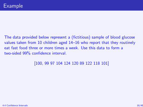
Example

The data provided below represent a (fictitious) sample of blood glucosevalues taken from 10 children aged 14–16 who report that they routinelyeat fast food three or more times a week. Use this data to form atwo-sided 99% confidence interval.

[100, 99 97 104 124 120 89 122 118 101]


Solution

Application of Equations 2.1 and 2.16 yield

x̄ =

∑x

n=

1074

10= 107.4

s =

√∑x2 − (

Px)2

n

n − 1=

√116732− (1074)2

10

10− 1=

√1384.4

9= 12.403.



Appendix B shows that the appropriate t value for a two-sided 99%confidence interval based on 10− 1 = 9 degrees of freedom is 3.250.Then by Equations 414 and 415

L = x̄ − ts√n

= 107.4− 3.25012.403√

10= 94.65

U = x̄ + ts√n

= 107.4 + 3.25012.403√

10= 120.15.


Assumptions

Assumptions underlying confidence intrvals for µ when σ is not known arethe same as those underlying the one mean t test which are the same asthose underlying the one mean Z test. Namely,

normality.

independence of observations.

Violating either or both of these assumptions may result in the level ofconfidence (coverage) actually realized being different from the intendedlevel.


Confidence Intervals For π

There are a number of approximate methods for constructingconfidence limits for a population proportion (π). However, thesemethods are often not sufficiently accurate for many applicationsespecially when the sample size (n) is not large or when p̂ is near zeroor one.

There is an exact method that overcomes this difficulty.


An Approximate Method

An approximation for L and U is given by the following.

L = p̂ − Z

√p̂q̂

n

U = p̂ + Z

√p̂q̂

n

Where p̂ is the proportion of successes in the sample of size n and q̂is the proportion of failures so that q̂ = 1− p̂. Z determines the levelof confidence and is found in the manner described in Section 4.4.4.


Example

Suppose a health policy researcher wishes to estimate the proportionof adults living in a rural southern county who have some form ofhealth insurance.

To this end, a sample of 350 adults living in the county areinterviewed.

Of the 350 persons interviewed, 112 or 112/350 = .32 report thatthey currently have some form of health insurance.

Form a two-sided 95% confidence interval to estimate the proportionof adults in the county who have health insurance.


Solution

L = p̂ − Z

√p̂q̂

n= .32− 1.96

√(.32) (.68)

350= .27

U = p̂ + Z

√p̂q̂

n= .32 + 1.96

√(.32) (.68)

350= .37.

Thus, the researcher can then be 95% confident that the proportionof adults living in the county who have health insurance is between.27 and .37.


Assumptions

Independence.

Normally distributed population (always violated).

A commonly invoked rule of thumb maintains that the normal curvemodel will be satisfactory so long as both nπ and n (1− π) aregreater than or equal to five. A more conservative rule states that thecriterion should be ten rather than five.


Exact Method

An exact confidence interval for the estimation of π can be formed asfollows.

L =S

S + (n − S + 1) FL

U =(S + 1) FU

n − S + (S + 1) FU

S is the number of successes in the sample, n is the number ofobservations in the sample and FL and FU are the appropriate valuesfrom an F distribution. FL and FU can be obtained from Appendix C.


Exact Method (continued)

The following notation is used for the degrees of freedom associated withthe F values used to calculate L and U.

dfLN – numerator degrees of freedom for calculating L.

dfLD – denominator degrees of freedom for calculating L.

dfUN – numerator degrees of freedom for calculating U.

dfUD – denominator degrees of freedom for calculating U.


Example

A random sample of 10 children with normal blood glucose levels whohave one or more siblings with diabetes are tested for antibodiesassociated with that disease.

Forty percent of these children test positive for the specified antibody.

Use the exact method to construct a two-sided 95% confidenceinterval to estimate the proportion of children of this type in thepopulation who will test positive for the antibody.


Solution

The degrees of freedom necessary to find FL can be found by noting thatthe number of successes (S) is np̂ = (10) (.4) = 4 and calculating,

dfLN = 2 (n − S + 1) = 2 (10− 4 + 1) = 14

dfLD = 2S = (2) (4) = 8.

Appendix C shows that with numerator degrees of freedom of 14 anddenominator degrees of freedom of 8, the appropriate F value to beused for the construction of a two-sided 95% confidence interval is4.13. Using this value gives

L =S

S + (n − S + 1) FL=

4

4 + (10− 4 + 1) 4.13= .122.


Solution (continuee)

The degrees of freedom for FU are

dfUN = 2 (S + 1) = 2 (4 + 1) = 10

dfUD = 2 (n − S) = 2 (10− 4) = 12.

The F value with numerator and denominator degrees of freedom of10 and 12 respectively to be used in the construction of a two-sided95% confidence interval is, by AppendixC, 3.37. Then,

U =(S + 1) FU

n − S + (S + 1) FU=

(4 + 1) 3.37

10− 4 + (4 + 1) 3.37= .737.

The exact two-sided 95% confidence interval is then .122 to .737.The sizable length of this interval is due to the small sample size.


Comparison Of HTs And CIs

Hypothesis tests and confidence intervals are closely related.

Confidence intervals can be used to perform hypothesis tests.

For this reason, and others, confidence intervals are usually preferableto hypothesis tests in situations where both might be employed.

4.5 Comparison Of HTs And CIs 32/40

Two-Tailed HT And Two-Sided CI

In general, a two-tailed hypothesis test to be conducted at level α canbe conducted by means of a two-sided confidence interval with levelof confidence level (1− α)× 100%.

Thus, to conduct a two-tailed test at α = .05 one can construct atwo-sided 95% CI.

If the value specified by the null hypothesis is between L and U, thenull hypothesis is not rejected. Otherwise, the null hypothesis isrejected.


Example

Suppose a researcher constructs a 99% CI to estimate µ in a situationwhere σ iis not known and finds L = 4 and U = 8.

Suppose the researcher, using the same data were to conduct atwo-tailed t test of the null hypothesis H0 : µ = 4.5 at α = .01, wouldthe t test reject or fail to reject the null hypothesis. Why?


Solution

We first note that level of confidence for the two-sided CI is(1− .01)× 100% = 99% which varifies that the CI can be used toconduct the hypothesis test.

Because µ0 = 4.5 is between L = 4 and U = 8, the null hypothesis ofthe hypothesis test would not be rejected.


One-Tailed HT And One-Sided CI

Just as two-sided confidence intervals can be used to performtwo-tailed hypothesis tests, so one-sided intervals can be used toconduct one-tailed tests.

For example, a test of a null hypothesis against an alternative of theform

HA : µ > µ0

can be conducted by forming a one-sided confidence interval for thelower bound of the estimated parameter.

If µ0 ≤ L the null hypothesis is rejected, otherwise it is not rejected.


One-Tailed HT And One-Sided CI (continued)

What form would a one-sided CI take if it were to be used as a test ofa null hypothesis against the alternative

HA : µ < µ0

Reversing the logic shown in Figure 4.31 on page 154, we see that thetest can be conducted by forming a one-sided confidence interval forthe upper bound of the estimated parameter. If µ0 ≥ U the nullhypothesis is rejected, otherwise it is not rejected.


Example

Use the information provided to perform the indicated hypothesis testvia the confidence interval method rather than the by the standardhypothesis test. How does this result compare with the resultobtained on page 95?

H0 : µ = 1000 σ = 235 x̄ = 985HA : µ < 1000 n = 180 α = .025


Solution

Because the test is one-tailed with an alternative that specifiesµ < 1000 we will perform the test by constructing a one-sidedconfidence interval for an upper bound estimate of µ.

By equation 4.13 on page 142,U = x̄ + Z σ√

n= 985 + 1.96 235√

180= 1019.33

Because U = 1019.33 > µ0 = 1000, the null hypothesis is notrejected. This is the same result obtained when the tes was done as aconventional test of hypothesis.


Some Additional Comments

Confidence intervals are generally more useful than are hypothesis testswhen both are applicable to a problem for the following reasons.

Confidence intervals can be used to perform hypothesis tests buthypothesis tests don’t produce confidence intervals.

Confidence intervals typically answer more interesting questions thando hypothesis tests. For example, what is µ rather than is µ differentfrom 12?

Hypothesis tests do not alert the researcher when sample sizes are toosmall (i.e. tests lack power) but confidence intervals do so byproducing unacceptably long intervals.


chapter four (continued) - biostatistics for the health ... · chapter four (continued) ......

Documents