chapter 8, sampling designs: random sampling, adaptive...
TRANSCRIPT

CHAPTER 8
SAMPLING DESIGNS - RANDOM SAMPLING, ADAPTIVE AND SYSTEMATIC
SAMPLING (Version 4, 14 March 2013) Page
8.1 SIMPLE RANDOM SAMPLING ....................................................................... 325
8.1.1 Estimation of Parameters ................................................................... 328 8.1.2 Estimation of a Ratio ........................................................................... 334 8.1.3 Proportions and Percentages............................................................ 337
8.2 STRATIFIED RANDOM SAMPLING ................................................................ 341
8.2.1 Estimates of Parameters ..................................................................... 343 8.22 Allocation of Sample Size .................................................................... 348 8.2.2.1 Proportional Allocation ................................................................ 348 8.2.2.2 Optimal Allocation ........................................................................ 350 8.2.3 Construction of Strata ......................................................................... 356 8.2.4 Proportions and Percentages............................................................. 359
8.3 ADAPTIVE SAMPLING .................................................................................... 360
8.3.1 Adaptive cluster sampling .................................................................. 361 8.3.2 Stratified Adaptive Cluster Sampling ................................................ 365
8.4 SYSTEMATIC SAMPLING ............................................................................... 365
8.5 MULTISTAGE SAMPLING ............................................................................... 369
8.5.1 Sampling Units of Equal Size ............................................................. 370 8.5.2 Sampling Units of Unequal Size ......................................................... 373
8.6 SUMMARY ....................................................................................................... 375
SELECTED REFERENCES ................................................................................... 377
QUESTIONS AND PROBLEMS ............................................................................. 378
Ecologists sample whenever they cannot do a complete enumeration of the population.
Very few plant and animal populations can be completely enumerated, and so most of
our ecological information comes from samples. Good sampling methods are critically

Chapter 8 Page 325
important in ecology because we want to have our samples be representative of the
population under study. How do we sample representatively? This chapter will attempt
to answer this question by summarizing the most common sampling designs that
statisticians have developed over the last 80 years. Sampling is a practical business
and there are two parts of its practicality. First, the gear used to gather the samples
must be designed to work well under field conditions. In all areas of ecology there has
been tremendous progress in the past 40 years to improve sampling techniques. I will
not describe these improvements in this book - they are the subject of many more
detailed handbooks. So if you need to know what plankton sampler is best for
oligotrophic lakes, or what light trap is best for nocturnal moths, you should consult the
specialist literature in your subject area. Second, the method of placement and the
number of samples must be decided, and this is what statisticians call sampling
design. Should samples be placed randomly or systematically? Should different
habitats be sampled separately or all together? These are the general statistical
questions I will address in this and the next chapter. I will develop a series of guidelines
that will be useful in sampling plankton with nets, moths with light traps, and trees with
distance methods. The methods discussed here are addressed in more detail by
Cochran (1977), Jessen (1978), and Thompson (1992).
8.1 SIMPLE RANDOM SAMPLING The most convenient starting point for discussing sampling designs is simple random
sampling. Like many statistical concepts, "random sampling" is easier to explain on
paper than it is to apply in the field. Some background is essential before we can
discuss random sampling. First, you must specify very clearly what the statistical
population is that you are trying to study. The statistical population may or may not be
a biological population, and the two ideas should not be confused. In many cases the
statistical population is clearly specified: the white-tailed deer population of the
Savannah River Ecological Area, or the whitefish population of Brooks Lake, or the
black oaks of Warren Dunes State Park. But in other cases the statistical population
has poorly defined boundaries: the mice that will enter live traps, the haddock
population of George’s Bank, the aerial aphid population over southern England, the
seed bank of Erigeron canadensis. Part of this vagueness in ecology depends on

Chapter 8 Page 326
spatial scale and has no easy resolution. Part of this vagueness also flows from the
fact that biological populations also change over time (Van Valen 1982). One strategy
for dealing with this vagueness is to define the statistical population very sharply on a
local scale, and then draw statistical inferences about it. But the biological population
of interest is usually much larger than a local population, and one must then
extrapolate to draw some general conclusions. You must think carefully about this
problem. If you wish to draw statistical inferences about a widespread biological
population, you should sample the widespread population. Only this way can you avoid
extrapolations of unknown validity. The statistical population you wish to study is a
function of the question you are asking. This problem of defining the statistical
population and then relating it to the biological population of interest is enormous in
field ecology, and almost no one discusses it. It is the first thing you should think about
when designing your sampling scheme.
Second, you must decide what the sampling unit, is in your population. The
sampling unit could be simple, like an individual oak tree or an individual deer, or it can
be more complex like a plankton sample, or a 4 m2 quadrat, or a branch of an apple
tree. The sample units must potentially cover the whole of the population and they
must not overlap. In most areas of ecology there is considerable practical experience
available to help decide what sampling unit to use.
The third step is to select a sample, and a variety of sampling plans can be
adopted. The aim of the sampling plan is to maximize efficiency - to provide the best
statistical estimates with the smallest possible confidence limits at the lowest cost. To
achieve this aim we need some help from theoretical statistics so that we can estimate
the precision and the cost of the particular sampling design we adopt. Statisticians
always assume that a sample is taken according to the principles of probability
sampling, as follows:
1. Define a set of distinct samples S1, S2, S3 ... in which certain specific sampling
units are assigned to S1, some to S2, and so on.
2. Each possible sample is assigned a probability of selection.

Chapter 8 Page 327
3. Select one of the Si samples by the appropriate probability and a random number
table.
If you collect a sample according to these principles of probability sampling, a
statistician can determine the appropriate sampling theory to apply to the data you
gather.
Some types of probability sampling are more convenient than others, and simple
random sampling is one. Simple random sampling is defined as follows:
1. A statistical population is defined that consists of N sampling units;
2. n units are selected from the possible samples in such a way that every unit
has an equal chance of being chosen.
The usual way of achieving simple random sampling is that each possible sample unit
is numbered from 1 to N. A series of random numbers between 1 and N is then drawn
either from a table of random numbers or from a set of numbers in a hat. The sample
units which happen to have these random numbers are measured and constitute the
sample to be analyzed. It is hard in ecology to follow these simple rules of random
sampling if you wish the statistical population to be much larger than the local area you
are actually studying.
Usually, once a number is drawn in simple random sampling it is not replaced, so
we have sampling without replacement. Thus, if you are using a table of random
numbers and you get the same number twice, you ignore it the second time. It is
possible to replace each unit after measuring so that you can sample with replacement
but this is less often used in ecology. Sampling without replacement is more precise
than sampling with replacement (Caughley 1977).
Simple random sampling is sometimes confused with other types of sampling that
are not based on probability sampling. Examples abound in ecology:
1. Accessibility sampling: the sample is restricted to those units that are readily
accessible. Samples of forest stands may be taken only along roads, or deer may be
counted only along trails.

Chapter 8 Page 328
2. Haphazard sampling: the sample is selected haphazardly. A bottom sample
may be collected whenever the investigator is ready, or ten dead fish may be picked up
for chemical analysis from a large fish kill.
3. Judgmental sampling: the investigator selects on the basis of his or her
experience a series of "typical" sample units. A botanist may select 'climax' stands of
grassland to measure.
4. Volunteer sampling: the sample is self-selected by volunteers who will
complete some questionnaire or be used in some physiological test. Hunters may
complete survey forms to obtain data on kill statistics.
The important point to remember is that all of these methods of sampling may give the
correct results under the right conditions. Statisticians, however, reject all of these
types of sampling because they can not be evaluated by the theorems of probability
theory. Thus the universal recommendation: random sample! But in the real world it is
not always possible to use random sampling, and the ecologist is often forced to use
non-probability sampling if he or she wishes to get any information at all. In some
cases it is possible to compare the results obtained with these methods to those
obtained with simple random sampling (or with known parameters) so that you could
decide empirically if the results were representative and accurate. But remember that
you are always on shaky ground if you must use non-probability sampling, so that the
means and standard deviations you calculate may not be close to the true values.
Whenever possible use some conventional form of random sampling.
8.1.1 Estimation of Parameters
In simple random sampling, one or more characteristics are measured on each
experimental unit. For example, in quadrat sampling you might count the number of
individuals of Solidago spp. and the number of individuals of Aster spp. In sampling
deer, you might record for each individual its sex, age, weight, and fat index. In
sampling starling nests you might count the number of eggs and measure their length.

Chapter 8 Page 329
In all these cases and in many more, ecological interest is focused on four
characteristics of the population1:
1. Total = X ; for example, the total number of Solidago individuals in the entire
100 ha study field.
2. Mean = x ; for example, the average number of Solidago per m2.
3. Ratio of two totals = R = x y ; for example, the number of Solidago per Aster in
the study area.
4. Proportion of units in some defined class; for example, the proportion of male
deer in the population.
We have seen numerous examples of characteristics of these types in the previous
seven chapters, and their estimation is covered in most introductory statistics books.
We cover them again here briefly because we need to add to them an idea that is not
usually considered in introductory books - the finite population correction. For any
statistical population consisting of N units, we define the finite population correction
(fpc) as:
fpc 1-N n nN N−
= = (8.1)
where:
fpc Finite population correction Total population size Sample size
Nn
===
and the fraction of the population sampled (n/N) is sometimes referred to as f. In a very
large population the finite population correction will be 1.0, and when the whole
population is measured, the fpc will be 0.0.
Ecologists working with abundance data such as quadrat counts of plant density
immediately run into a statistical problem at this point. Standard statistical procedures
1 We may also be interested in the variance of the population, and the same general
procedures apply.

Chapter 8 Page 330
deal with normally distributed raw data in which the standard deviation is independent
of the mean. But ecological abundance data typically show a positive skew (e.g. Figure
4.6 page 000) with the standard deviation increasing with the mean. These
complications violate the assumptions of parametric statistics, and the simplest way of
correcting ecological abundance data is to transform all counts by a log transformation:
( )logY X= (8.2)
where Y = transformed data
X = original data
All analysis is now done on these Y-values which tend to satisfy the assumptions of
parametric statistics1. In the analyses that follow with abundance data we effectively
replace all the observed X values with their Y transformed counterpart and use the
conventional statistical formulas found in most textbooks that define the variable of
interest as X.
Cochran (1977) demonstrates that unbiased estimates of the population mean
and total for normally distributed data are given by the following formulas. For the
mean:
ixx
n= ∑ (8.3)
where:
= Population mean = Observed value of in sample = Sample size
i
xx x in
For the variance2 of the measurements we have the usual formula:
( )2
2
1ix x
sn
−=
−∑ (8.4)
1 This transformation will be discussed in detail in Chapter 15, page 000.
2 If the data are compiled in a frequency distribution, the appropriate formulas are supplied in Appendix 1, page 000.

Chapter 8 Page 331
and the standard error of the population mean x is given by:
( )2
1xss fn
= − (8.5)
where:
2 Standard error of the mean Variance of the measurements as defined above (8.4) Sample size Sampling fraction /
xs xsnf n N
==== =
These formulas are similar to those you have always used, except for the introduction
of the finite population correction. Note that when the sampling fraction (n/N) is low, the
finite population correction is nearly 1.0 and so the size of the population has no effect
on the size of the standard error. For example, if you take a sample of 500
measurements from two populations with the same variance ( 2s = 484.0) and
population A is small (N = 10,000) and population B is a thousand times larger (N =
10,000,000), the standard errors of the mean differ by only 2.5% because of the finite
population correction. For this reason, the finite population correction is usually ignored
whenever the sampling fraction (n/N) is less than 5% (Cochran 1977).
Estimates of the population total are closely related to these formulas for the
population mean. For the population total:
X̂ N x= (8.6)
where: ˆ Estimated population total
Total size of population Mean value of population
XNx
===
The standard error of this estimate is given by:
X xs N s= (8.7)
where:
= Standard error of the population total = Total size of the population = Standard error of the mean from equation (8.4)
X
x
sNs
Confidence limits for both the population mean and the population total are usually
derived by the normal approximation:

Chapter 8 Page 332
xx t sα± (8.8)
where:
( ) = Student's value for - 1 degrees of freedom for the
1- level of confidencet t nα
α
This formula is used all the time in statistics books with the warning not to use it except
with "large" sample sizes. Cochran (1977, p.41) gives a rule-of-thumb that is useful for
data that has a strong positive skew (like the negative binomial curves in Figure 4.8,
page 000). First, define Fisher’s measure of skewness:
( )1
33
Fisher's measure of skewness1
g
x xns
=
= −∑ (8.9)
Cochran’s rule is that you have a large enough sample to use the normal
approximation (equation 8.8) if –
2125n g> (8.10)
where:
= Sample size = Standard deviation
ns
Sokal and Rohlf (1995, p. 116) show how to calculate g1 from sample data and many
statistical packages provide computer programs to do these calculations.
Box 8.1 (page 000) illustrates the use of these formulae for simple random
sampling.
Box 8.1 ESTIMATION OF POPULATION MEAN AND POPULATION TOTAL FROM SIMPLE RANDOM SAMPLING OF A FINITE POPULATION
A biologist obtained body weights of male reindeer calves from a herd during the seasonal roundup. He obtained weights on 315 calves out of a total of 1262 in the herd, checked the assumption of a normal distribution, and summarized the data:
Body weight class (kg)
Midpoint, x Observed frequency, fx
29.5-34.5 32 4 34.5-39.5 37 13 39.5-44.5 42 20 44.5-49.5 47 49 49.5-54.5 52 61

Chapter 8 Page 333
54.5-59.5 57 72 59.5-64.5 62 57 64.5-69.5 67 25 69.5-74.5 72 12 74.5-79.5 77 2
The observed mean is, from the grouped version of equation (8.3),
(4)(32) + (13)(37) + (20)(42) + 315
17,255 = = 54.78 kg315
xf xx
n= =∑
The observed variance is, from the grouped version of equation (8.4),
( )222
2
/ - 1
969,685 - (17,255) / 315 78.008314
x xf x f x ns
n−
=
= =
∑ ∑
The standard error of the mean weight, from equation (8.5): 2
1
78.008 315 1- 0.4311315 1262
xss fn
= −
= =
From equation (8.8) we calculate g1 = ( ) ( )331/ ns x x−∑ = -0.164. Hence, applying equation (8.10)
21
225
315 25( 0.164) 0.67n g>
>> − =
so that we have a “large” sample according to Cochran’s rule of thumb. Hence we can compute normal confidence limits from equation (8.8): for α = .05 the t value for 315 d.f. is 1.97
xx t sα±
54.78 1.97(0.431)±
or 95% confidence limits of 53.93 to 55.63 kg. To calculate the population total biomass, we have from equation (8.6):

Chapter 8 Page 334
ˆ 1262 (54.78) 69,129.6 kgX N x= = =
and the standard error of this total biomass estimate for the herd is, from equation (8.7),
ˆ 1262(0.4311) 544.05xXs N s= = =
and normal 95% confidence limits can be calculated as above to give for the population total:
69,130 1072 kg±
It is important to remember that if you have carried out a log transform on
abundance data, all of these estimates are in the log-scale. You may wish to transform
them back to the original scale of measurement, and this procedure is not immediately
obvious (i.e. do not simply take anti-logs) and is explained in Chapter 15, Section
15.1.1 (page 000).
8.1.2 Estimation of a Ratio
Ratios are not as commonly used in ecological work as they are in taxonomy, but
sometimes ecologists wish to estimate from a simple random sample a ratio of two
variables, both of which vary from sampling unit to sampling unit. For example, wildlife
managers may wish to estimate the wolf/moose ratio for several game management
zones, or behavioral ecologists may wish to measure the ratio of breeding females to
breeding males in a bird population. Ratios are peculiar statistical variables with
strange properties that few biologists appreciate (Atchley et al. 1976). Ratios of two
variables are not just like ordinary measurements and to estimate means, standard
errors, and confidence intervals for ecological ratios, you should use the following
formulae from Cochran (1977):
For the mean ratio:
ˆ xRy
= (8.11)
where:

Chapter 8 Page 335
ˆ Estimated mean ratio of to Observed mean value of Observed mean value of
R x yx xy y
===
The standard error of this estimated ratio is:
2 2 2
ˆ
ˆ ˆ211R
x R xy R yfs
nn y− +−
=−
∑ ∑ ∑ (8.12)
where:
ˆ Estimated standard error of the ratio Sampling fraction / Sample size Observed mean of measurement (denominator of ratio)
Rs R
f n Nny Y
== ===
and the summation terms are the usual ones defined in Appendix 1 (page 000).
The estimation of confidence intervals for ratios from the usual normal
approximation (eq. 8.8) is not valid unless sample size is large as defined above (page
332) (Sukhatme and Sukhatme 1970). Ratio variables are often skewed to the right
and not normally distributed, particularly when the coefficient of variation of the
denominator is relatively high (Atchley et al. 1976). The message is that you should
treat the computed confidence intervals of a ratio as only an approximation unless
sample size is large.
Box 8.2 illustrates the use of these formulas for calculating a ratio estimate.
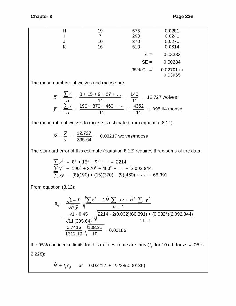
Box 8.2 ESTIMATION OF A RATIO OF TWO VARIABLES FROM SIMPLE RANDOM SAMPLING OF A FINITE POPULATION
Wildlife ecologists interested in measuring the impact of wolf predation on moose populations in British Columbia obtained estimates by aerial counting of the population size of wolves and moose and 11 subregions which constituted 45% of the total game management zone.
Subregion No. of wolves No. of moose Wolves/moose A 8 190 0.0421 B 15 370 0.0405 C 9 460 0.0196 D 27 725 0.0372 E 14 265 0.0528 F 3 87 0.0345 G 12 410 0.0293
Chapter 8 Page 336
H 19 675 0.0281 I 7 290 0.0241 J 10 370 0.0270 K 16 510 0.0314
x = 0.03333 SE = 0.00284 95% CL = 0.02701 to
0.03965
The mean numbers of wolves and moose are
8 + 15 + 9 + 27 + 140 12.727 wolves11 11
190 + 370 + 460 + 4352 395.64 moose11 11
xx
ny
yn
= = = =
= = = =
∑
∑
The mean ratio of wolves to moose is estimated from equation (8.11):
12.727ˆ 0.03217 wolves/moose395.64
xRy
= = =
The standard error of this estimate (equation 8.12) requires three sums of the data:
2 2 2 2
2 2 2 2 8 + 15 + 9 + 2214
y 190 + 370 + 460 + 2,092,844 (8)(190) + (15)(370) + (9)(460) + 66,391
x
xy
= == == =
∑∑∑
From equation (8.12):
2 2 2
ˆ
2
ˆ ˆ211
1 - 0.45 2214 - 2(0.032)(66,391) + (0.032 )(2,092,844) 11 - 111 (395.64)
0.7416 108.31 0.001861312.19 10
R
x R xy R yfs
nn y− +−
=−
=
= =
∑ ∑ ∑
the 95% confidence limits for this ratio estimate are thus ( tα for 10 d.f. for α = .05 is
2.228):
ˆ or 0.03217 2.228(0.00186)RR t sα± ±

Chapter 8 Page 337
or 0.02803 to 0.03631 wolves per moose.
8.1.3 Proportions and Percentages
The use of proportions and percentages is common in ecological work. Estimates of
the sex ratio in a population, the percentage of successful nests, the incidence of
disease, and a variety of other measures are all examples of proportions. In all these
cases we assume there are 2 classes in the population, and all individuals fall into one
class or the other. We may be interested in either the number or the proportion of type
X individuals from a simple random sample:
Population Sample
No. of total individuals N n
No. of individuals of type X A a
Proportion of type X individuals
AP N= ˆ ap n=
In statistical work the binomial distribution is usually applied to samples of this type, but
when the population is finite the more proper distribution to use is the hypergeometric
distribution1 (Cochran 1977). Fortunately, the binomial distribution is an adequate
approximation for the hypergeometric except when sample size is very small.
For proportions, the sample estimate of the proportion P is simply:
ˆ ap n= (8.13)
where:
ˆ Proportion of type individuals Number of type individuals in sample Sample size
p Xa Xn
===
The standard error of the estimated proportion p̂ is from Cochran (1977),
ˆˆ ˆ
11P
pqs fn
= −−
(8.14)
1 Zar (1996, pg. 520) has a good brief description of the hypergeometric distribution.

Chapter 8 Page 338
where:
ˆ = Standard error of the estimated population Sampling fraction /
ˆ Estimated proportion of typesˆ ˆ 1 -
Sample size
Ps pf n Np Xq pn
= ====
For example, if in a population of 3500 deer, you observe a sample of 850 of which
400 are males:
ˆ
ˆ 400/850 0.4706850 (0.4706)(1 - 0.4706) 1 0.0149
3500 849P
p
s
= =
= − =
To obtain confidence limits for the proportion of x-types in the population several
methods are available (as we have already seen in Chapter 2, page 000). Confidence
limits can be read directly from graphs such as Figure 2.2 (page 000), or obtained
more accurately from tables such as Burnstein (1971) or from Program EXTRAS
(Appendix 2, page 000). For small sample sizes the exact confidence limits can be
read from tables of the hypergeometric distribution in Lieberman and Owen (1961).
If sample size is large, confidence limits can be approximated from the normal
distribution. Table 8.1 lists sample sizes that qualify as "large". The normal
approximation to the binomial gives confidence limits of:
ˆ ˆ 1ˆ 11 2
pqp z fn nα
± − + −
or
ˆ1ˆ
2Pp z s
nα ± +
(8.15)
where:

Chapter 8 Page 339
ˆ
ˆ = Estimated proportion of types = Standard normal deviate (1.96 for 95% confidence intervals, 2.576
for 99% confidence intervals) Standard error of the estimated proportion (equat
P
p Xz
s
α
= ion 8.13) Sampling fraction /
ˆ ˆ 1 - proportion of types in sample Sample size
f n Nq p Yn
= == ==
TABLE 8.1 SAMPLE SIZES NEEDED TO USE THE NORMAL APPROXIMATION (EQUATION 8.15) FOR CALCULATING CONFIDENCE INTERVALS FOR PROPORTIONSa
Proportion, p
Number of individuals in the smaller class,
np
Total sample size, N
0.5 15 30 0.4 20 50 0.3 24 80 0.2 40 200 0.1 60 600
0.05 70 1400
a For a given value of p do not use the normal approximation unless you have a sample size this large or larger. Source: Cochran, 1977.
The fraction (1/2n) is a correction for continuity, which attempts to correct partly for the
fact that individuals come in units of one, so it is possible, for example, to observe 216
male deer or 217, but not 216.5. Without this correction the normal approximation
usually gives a confidence belt that is too narrow.
For the example above, the 95% confidence interval would be:
10.4706 1.96(0.0149)2(850)
or 0.4706 0.0298 (0.44 to 0.50 males)
± + ±
Note that the correction for continuity in this case is very small and if ignored would not
change the confidence limits except in the fourth decimal place.
Chapter 8 Page 340
Not all biological attributes come as two classes like males and females of
course, and we may wish to estimate the proportion of organisms in three or four
classes (instar I, II, III and IV in insects for example). These data can be treated most
simply by collapsing them into two-classes, instar II vs. all other instars for example,
and using the methods described above. A better approach is described in Section
13.4.1 for multinomial data.
One practical illustration of the problem of estimating proportions comes from
studies of disease incidence (Ossiander and Wedemeyer 1973). In many hatchery
populations of fish, samples need to be taken periodically and analyzed for disease.
Because of the cost and time associated with disease analysis, individual fish are not
always the sampling unit. Instead, groups of 5, 10 or more fish may be pooled and the
resulting pool analyzed for disease. One diseased fish in a group of 10 will cause that
whole group to be assessed as disease-positive. Worlund and Taylor (1983)
developed a method for estimating disease incidence in populations when samples are
pooled. The sampling problem is acute here because disease incidence will often be
only 1-2%, and at low incidences of disease, larger group sizes are more efficient in
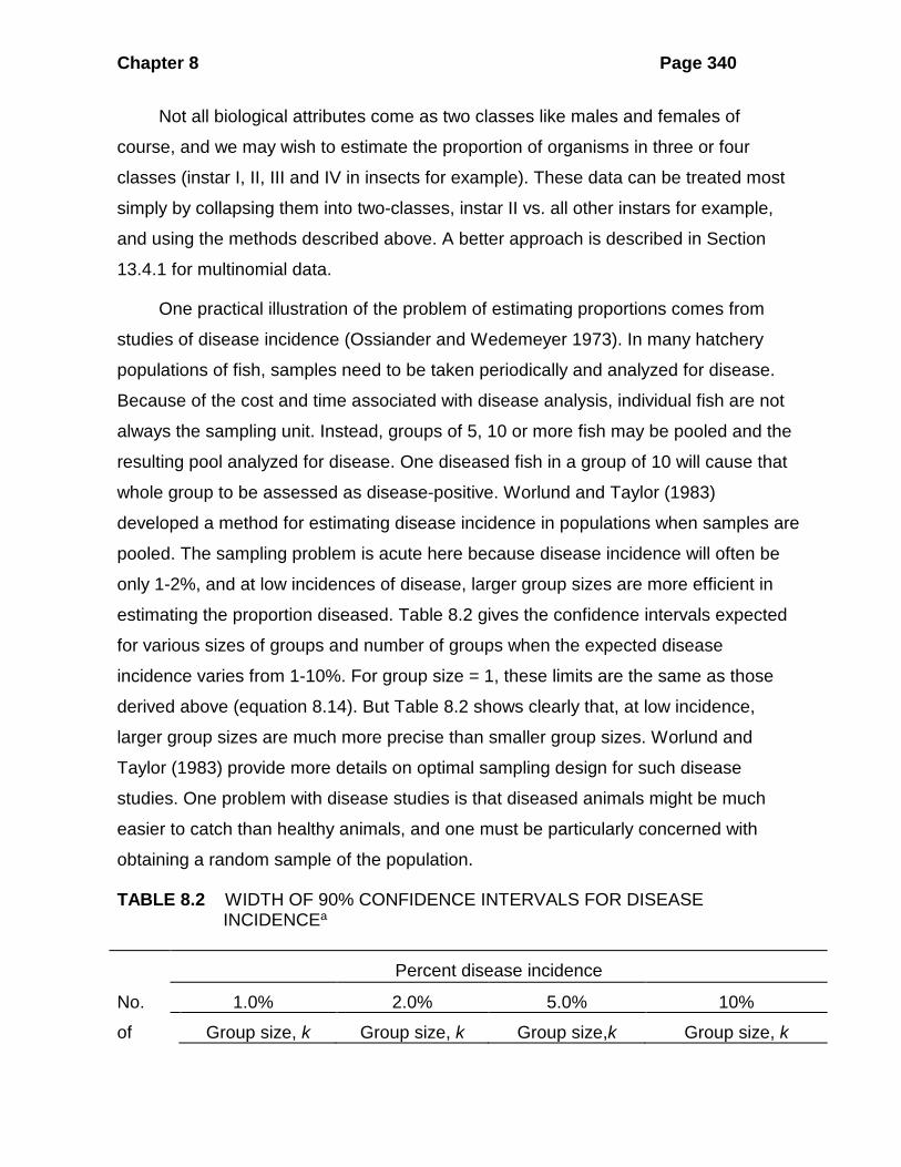
estimating the proportion diseased. Table 8.2 gives the confidence intervals expected
for various sizes of groups and number of groups when the expected disease
incidence varies from 1-10%. For group size = 1, these limits are the same as those
derived above (equation 8.14). But Table 8.2 shows clearly that, at low incidence,
larger group sizes are much more precise than smaller group sizes. Worlund and
Taylor (1983) provide more details on optimal sampling design for such disease
studies. One problem with disease studies is that diseased animals might be much
easier to catch than healthy animals, and one must be particularly concerned with
obtaining a random sample of the population.
TABLE 8.2 WIDTH OF 90% CONFIDENCE INTERVALS FOR DISEASE INCIDENCEa
Percent disease incidence
No. 1.0% 2.0% 5.0% 10%
of Group size, k Group size, k Group size,k Group size, k

Chapter 8 Page 341
groups,
n 1 5 10 159 1 5 10 79 1 5 10 31 1 5 10 15 12 4.7 2.1 1.5 - 6.6 3.0 2.2 - 10.3 4.9 3.7 - 14.2 7.1 - -
20 3.6 1.6 1.2 - 5.1 2.3 1.7 - 8.0 3.8 2.8 - 11.0 5.5 4.5 -
30 3.0 1.3 1.0 0.4 4.2 1.9 1.4 0.7 6.5 3.1 2.3 1.8 9.0 4.5 3.7 3.5
60 2.1 1.0 0.7 0.3 3.0 1.4 1.0 0.5 4.6 2.2 1.6 1.3 6.4 3.2 2.6 2.5
90 1.7 0.8 0.6 0.2 2.4 1.1 0.8 0.4 3.8 1.8 1.3 1.0 5.2 2.6 2.1 2.0
120 1.5 0.7 0.5 0.2 2.1 1.0 0.7 0.4 3.3 1.5 1.2 0.8 4.5 2.2 1.8 1.8
150 1.3 0.6 0.4 0.2 1.9 0.8 0.6 0.3 2.9 1.4 1.0 0.8 4.0 2.0 1.6 1.6
250 1.0 0.5 0.3 0.1 1.4 0.7 0.5 0.2 2.3 1.1 0.8 0.6 3.1 1.6 1.3 1.2
350 0.9 0.4 0.3 0.1 1.2 0.6 0.4 0.2 1.9 0.9 0.7 0.5 2.6 1.3 1.1 1.0
450 0.8 0.3 0.2 0.1 1.1 0.5 0.4 0.2 1.7 0.8 0.6 0.5 2.3 1.2 1.0 0.9
a A number of groups (n) of group size k are tested for disease. If one individual in a group has a disease, the whole group is diagnosed as disease positive. The number in the table should be read as “ %d± ,” that is, as one-half of the width of the confidence interval. Source: Worlund and Taylor, 1983.
8.2 STRATIFIED RANDOM SAMPLING One of the most powerful tools you can use in sampling design is to stratify your
population. Ecologists do this all the time intuitively. Figure 8.1 gives a simple example.
Population density is one of the most common bases of stratification in ecological
work. When an ecologist recognizes good and poor habitats, he or she is implicitly
stratifying the study area.
In stratified sampling the statistical population of N units is divided into
subpopulations which do not overlap and which together comprise the entire
population. Thus:
N = N1 + N2 + N3 + ..... NL
where L = total number of subpopulations

Chapter 8 Page 342
Stratum C
Stratum B
Stratum A
Figure 8.1 The idea of stratification in estimating the size of a plant or animal population. Stratification is made on the basis of population density. Stratum A has about ten times the density of Stratum C.
The subpopulations are called strata by statisticians. Clearly if there is only one
stratum, we are back to the kind of sampling we have discussed earlier in this chapter.
To obtain the full benefit from stratification you must know the sizes of all the strata
(N1, N2, ...). In many ecological examples, stratification is done on the basis of
geographical area, and the sizes of the strata are easily found in m2 or km2, for
example. There is no need for the strata to be of the same size.
Once you have determined what the strata are, you sample each stratum
separately. The sample sizes for each stratum are denoted by subscripts:
n1 = sample size in stratum 1 n2 = sample size in stratum 2 and so on. If within each stratum you sample using the principles of simple random
sampling outlined above (page 327), the whole procedure is called stratified random
sampling. It is not necessary to sample each stratum randomly, and you could, for
example, sample systematically within a stratum. But the problems outlined above
would then mean that it would be difficult to estimate how reliable such sampling is. So
it is recommended to sample randomly within each stratum.

Chapter 8 Page 343
Ecologists have many different reasons for wishing to stratify their sampling. Four
general reasons are common (Cochran 1977):
1. Estimates of means and confidence intervals may be required separately for each subpopulation.
2. Sampling problems may differ greatly in different areas. Animals may be easier or harder to count in some habitats than they are in others. Offshore samples may require larger boats and be more expensive to get than nearshore samples.
3. Stratification may result in a gain in precision in the estimates of the parameters of the whole population. Confidence intervals can be narrowed appreciably when strata are chosen well.
4. Administrative convenience may require stratification if different field laboratories are doing different parts of the sampling.
Point 3 is perhaps the most critical one on this list, and I will now discuss how
estimates are made from stratified sampling and illustrate the gains one can achieve.
8.2.1 Estimates of Parameters
For each of the subpopulations (N1, N2, ...) all of the principles and procedures of
estimation outlined above can be used. Thus, for example, the mean for stratum 1 can
be estimated from equation (8.2) and the variance from equation (8.3). New formulas
are however required to estimate the mean for the whole population N. It will be
convenient, before I present these formulae, to outline one example of stratified
sampling so that the equations can be related more easily to the ecological framework.
Table 8.3 gives information on a stratified random sample taken on a caribou
herd in central Alaska by Siniff and Skoog (1964). They used as their sampling unit a
quadrat of 4 sq. miles, and they stratified the whole study zone into six strata, based on
a pilot survey of caribou densities in different regions. Table 8.3 shows that the 699
total sampling units were divided very unequally into the six strata, so that the largest
stratum (A) was 22 times the size of the smallest stratum (D).

Chapter 8 Page 344
TABLE 8.3 STRATIFIED RANDOM SAMPLING OF THE NELCHINA CARIBOU HERD IN ALASKA BY SINIFF AND SKOOG (1964)a
Stratum Stratum size, Nh Stratum weight, Wh
Sample size, nh Mean no. of caribou counted
per sampling unit, hx
Variance of Caribou counts,
2hs
A 400 0.572 98 24.1 5575 B 30 0.043 10 25.6 4064 C 61 0.087 37 267.6 347,556 D 18 0.026 6 179.0 22,798 E 70 0.100 39 293.7 123,578 F 120 0.172 21 33.2 9795
Total 699 1.000 211 a Six strata were delimited in preliminary surveys based on the relative caribou density. Each sampling unit was 4 square miles. A random sample was selected in each stratum and counts were made from airplanes. Source: Siniff and Skoog, 1964.
We define the following notation for use with stratified sampling:
Stratum weight = = hh
NWN
(8.16)
where:
Nh = Size of stratum h (number of possible sample units in stratum h)
N = Size of entire statistical population
The stratum weights are proportions and must add up to 1.0 (Table 8.3). Note that the
Nh must be expressed in "sample units". If the sample unit is 0.25 m2, the sizes of the
strata must be expressed in units of 0.25 m2 (not as hectares, or km2).
Simple random sampling is now applied to each stratum separately and the
means and variances calculated for each stratum from equations (8.2) and (8.3). We
will defer until the next section a discussion on how to decide sample size in each
stratum. Table 8.3 gives sample data for a caribou population.
Chapter 8 Page 345
The overall mean per sampling unit for the entire population is estimated as
follows (Cochran 1977):
1ST =
L
h hh
N xx
N=∑
(8.17)
where:
ST = Stratified population mean per sampling unit = Size of stratum = Stratum number (1, 2, 3, , ) = Observed mean for stratum = Total population size =
h
h
h
xN h
h Lx hN N∑
Note that STx is a weighted mean in which the stratum sizes are used as weights.
For the data in Table 8.3, we have:
ST(400)(24.1) + (30)(25.6) + (61)(267.6 + =
699 = 77.96 caribou/sample unit
x
Given the density of caribou per sampling unit, we can calculate the size of the entire
caribou population from the equation:
ST STˆ = X N x (8.18)
where:
ST
ST
ˆ Population total Number of sample units in entire population
x Stratified mean per sampling unit (equation 8.17)
XN
===
For the caribou example:
STˆ = 699(77.96) = 54,497 caribouX
so the entire caribou herd is estimated to be around 55 thousand animals at the time of
the study.
The variance of the stratified mean is given by Cochran (1977, page 92) as:

Chapter 8 Page 346
( ) ( )2 2
ST1
Variance of 1L
h hh
h h
w sx fn=
= −
∑ (8.19)
where:
2
/
Stratum weight (equation 8.16) Observed variance of stratum (equation 8.4) Sample size in stratum Sampling fraction in stratum /
h
h
h
h h h
Ws hn hf h n N
==== =
The last term in this summation is the finite population correction and it can be ignored
if you are sampling less that 5% of the sample units in each stratum. Note that the
variance of the stratified means depends only on the size of the variances within each
stratum. If you could divide a highly variable population into homogeneous strata such
that all measurements within a stratum were equal, the variance of the stratified mean
would be zero, which means that the stratified mean would be without any error! In
practice of course you cannot achieve this but the general principle still pertains: pick
homogeneous strata and you gain precision.
For the caribou data in Table 8.3 we have:
( )
( )
2
ST
2
(0.572) (5575) 98Variance of = 1 - 98 400
(0.043) 4064 10 + 1 - + 10 30
= 69.803
x
The standard error of the stratified mean is the square root of its variance:
( )ST STStandard error of = Variance of = 69.803 = 8.355x x
Note that the variance of the stratified mean cannot be calculated unless there are at
least 2 samples in each stratum. The variance of the population total is simply:
( ) ( ) ( )2ST ST
ˆVariance of = variance of X N x (8.20)
For the caribou the variance of the total population estimate is:
( ) 2ST
ˆVariance of = 699 (69.803) 34,105,734X =

Chapter 8 Page 347
and the standard error of the total is the square root of this variance, or 5840.
The confidence limits for the stratified mean and the stratified population total are
obtained in the usual way:
ST ST (standard error of )x t xα± (8.21)
ST STˆ ˆ (standard error of )X t Xα± (8.22)
The only problem is what value of Student's t to use. The appropriate number of
degrees of freedom lies somewhere between the lowest of the values (nh - 1) and the
total sample size ( 1hn −∑ ). Cochran (1977, p.95) recommends calculating an effective
number of degrees of freedom from the approximate formula:
( )
22
12 4
1
d.f.
1
L
h hh
Lh h
hh
g s
g sn
−
−
≈ −
∑
∑ (8.23)
where:
( )2
d.f. Effective number of degrees of freedom for the confidence limits in equations (8.21) and (8.22)
/ Observed variance in stratum Sample size in stratum S
h h h h h
h
h
h
g N N n ns hn hN
=
= −=== ize of stratum h
For example, from the data in Table 8.3 we obtain
Stratum gh
A 1232.65
B 60.00
C 39.57
D 36.00
E 55.64
F 565.71

Chapter 8 Page 348
and from equation (8.22):
2
12(34,106,392)d.f. = 134.38.6614 X 10
≈
and thus for 95% confidence intervals for this example tα = 1.98. Thus for the
population mean from equation (8.20) the 95% confidence limits are:
77.96 1.98(8.35)±
or from 61.4 to 94.5 caribou per 4 sq. miles. For the population total from equation
(8.21) the 95% confidence limits are:
54,497 1.98(5840)±
or from 42,933 to 66,060 caribou in the entire herd.
8.22 Allocation of Sample Size
In planning a stratified sampling program you need to decide how many sample units
you should measure in each stratum. Two alternate strategies are available for
allocating samples to strata - proportional allocation or optimal allocation.
8.2.2.1 Proportional Allocation
The simplest approach to stratified sampling is to allocate samples to strata on the
basis of a constant sampling fraction in each stratum. For example, you might decide
to sample 10% of all the sample units in each stratum. In the terminology defined
above:
h hn Nn N
= (8.24)
For example, in the caribou population of Table 8.3, if you wished to sample 10% of
the units, you would count 40 units in stratum A, 3 in stratum B, 6 in stratum C, 2 in
stratum D, 7 in E and 12 in F. Note that you should always constrain this rule so that at
least 2 units are sampled in each stratum so that variances can be estimated.
Equation (8.23) tells us what fraction of samples to assign to each stratum but we
still do not know how many samples we need to take in total (n). In some situations this
Chapter 8 Page 349
is fixed and beyond control. But if you are able to plan ahead you can determine the
sample size you require as follows.
• Decide on the absolute size of the confidence interval you require in the final estimate. For example, in the caribou case you may wish to know the density to ±10 caribou/4 sq. miles with 95% confidence.
• Calculate the estimated total number of samples needed for an infinite population from the approximate formula (Cochran 1977 p. 104):
2
2
4 h hW sn
d≈ ∑ (8.25)
where:
2
Total sample size required (for large population) Stratum weight Observed variance of stratum Desired absolute precision of stratified mean (width of confidence
interval
h
h
nWs hd
====
is )d±
This formula is used when 95% confidence intervals are specified in d. If 99%
confidence intervals are specified, replace 4 in equation (8.24) with 7.08, and for 90%
confidence intervals, use 2.79 instead of 4. For a finite population correct this
estimated n by equation (7.6), page 000:
* = 1
nn nN+
where:
* = Total sample size needed in finite population of size n N
For the caribou data in Table 8.3, if an absolute precision of ± 10 caribou / 4 square
miles is needed:
[ ]2
4 (0.572)(5575) + (0.043)(4064) + 1 = 1933.6
10n ≈
Note that this recommended sample size is more than the total sample units available!
For a finite population of 699 sample units:

Chapter 8 Page 350
1933.6 513.4 sample units1933.61 + 699n∗ ≈ =
These 514 sample units would then be distributed to the six strata in proportion to the
stratum weight. Thus, for example, stratum A would be given (0.572)(514) or 294
sample units. Note again the message that if you wish to have high precision in your
estimates, you will have to take a large sample size.
8.2.2.2 Optimal Allocation
When deciding on sample sizes to be obtained in each stratum, you will find that
proportional allocation is the simplest procedure. But it is not the most efficient, and if
you have prior information on the sampling methods, more powerful allocation plans
can be specified. In particular, you can minimize the cost of sampling with the following
general approach developed by Cochran (1977).
Assume that you can specify the cost of sampling according to a simple cost
function:
O h hC c c n= + ∑ (8.26)
where:
O
Total cost of sampling Overhead cost Cost of taking one sample in stratum Number of samples taken in stratum
h
h
Ccc hn h
====
Of course the cost of taking one sample might be equal in all strata but this is not
always true. Costs can be expressed in money or in time units. Economists have
developed much more complex cost models but we shall stick to this simple model
here.
Cochran (1977 p. 95) demonstrates that, given the cost function above, the
standard error of the stratified mean is at a minimum when:
is proportional to h hh
h
N snc

Chapter 8 Page 351
This means that we should apportion samples among the strata by the ratio:
//
h h hh
h h h
N s cnn N s c
= ∑
(8.27)
This formula leads to three useful rules-of-thumb in stratified sampling: in a given
stratum, take a larger sample if
1. The stratum is larger
2. The stratum is more variable internally
3. Sampling is cheaper in the stratum
Once we have done this we can now go in one of two ways:
(1) minimize the standard error of the stratified mean for a fixed total cost. If the
cost is fixed, the total sample size is dictated by:
( ) ( )( )
O /h h h
h h h
C c N s cn
N s c
−=
∑∑
(8.28)
where:
O
Total sample size to be used in stratified sampling for all strata combined Total cost (fixed in advance) Overhead cost Size of stratum standard deviation of stratum cost to
h
h
h
nC
cN hs hc
====== take one sample in stratum h
Box 8.3 illustrates the use of these equations for optimal allocation.
Box 8.3 OPTIMAL AND PROPORTIONAL ALLOCATION IN STRATIFIED RANDOM SAMPLING
Russell (1972) sampled a clam population using stratified random sampling and obtained the following data: Stratum Size of
stratum, Nh Stratum
weight, Wh Sample size,
nh Mean
(bushels), xh Variance, 2
hs
A 5703.9 0.4281 4 0.44 0.068 B 1270.0 0.0953 6 1.17 0.042 C 1286.4 0.0965 3 3.92 2.146

Chapter 8 Page 352
D 5063.9 0.3800 5 1.80 0.794 N = 13,324.2 1.0000 18
Stratum weights are calculated as in equation (8.16). I use these data to illustrate hypothetically how to design proportional and optimal allocation sampling plans. Proportional Allocation If you were planning this sampling program based on proportional allocation, you would allocate the samples in proportion to stratum weight (equation 8.24): Stratum Fraction of samples to be
allocated to this stratum
A 0.43 B 0.10 C 0.10 D 0.38
Thus, if sampling was constrained to take only 18 samples (as in the actual data), you would allocate these as 7, 2, 2, and 7 to the four strata. Note that proportional allocation can never be exact in the real world because you must always have two samples in each stratum and you must round off the sample sizes. If you wish to specify a level of precision to be attained by proportional allocation, you proceed as follows. For example, assume you desire an absolute precision of the stratified mean of d = ± 0.1 bushels at 95% confidence. From equation (8.25):
[ ]2
2 2
4 4 (0.4281)(0.068) (0.0953)(0.042) + (0.1)
217 samples
h hW sn
d+
≈ =
≈
∑
(assuming the sampling fraction is negligible in all strata). These 217 samples would be distributed to the four strata according to the fractions given above - 43% to stratum A, 10% to stratum B, etc. Optimal Allocation In this example proportional allocation is very inefficient because the variances are very different in the four strata, as well as the means. Optimal allocation is thus to be preferred. To illustrate the calculations, we consider a hypothetical case in which the cost per sample varies in the different strata. Assume that the overhead cost in equation (8.25) is $100 and the coasts per sample are
c1 = $10 c2 = $20 c3 = $30 c4 = $40
Apply equation (8.27) to determine the fraction of samples in each stratum:

Chapter 8 Page 353
//
h h hh
h h h
N s cnn N s c
=∑
These fractions are calculated as follows: Stratum Nh sh
hc /h hN s c
Estimated fraction, nh/n
A 5703.9 0.2608 3.162 470.35 0.2966 B 1270.0 0.2049 4.472 58.20 0.0367 C 1286.4 1.4649 5.477 344.06 0.2169 D 5063.9 0.8911 6.325 713.45 0.4498
Total = 1586.06 1.0000 We can now proceed to calculate the total sample size needed for optimal allocation under two possible assumptions: Minimize the Standard Error of the Stratified Mean In this case cost is fixed. Assume for this example that $200 is available. Then, from equation (8.28),
( )
( )O /
/(2000 - 100)(1586.06) 70.9 (rounded to 71 samples)
44,729.745
h h h
h h h
C c N s cn
N s c
− =
= =
∑
∑
Note that only the denominator needs to be calculated, since we have already computed the numerator sum. We allocate these 71 samples according to the fractions just established: Stratum Fraction of
samples Total no. samples
allocation of 68 total
A 0.2966 21.1 (21) B 0.0367 2.6 (3) C 0.2169 15.4 (15) D
0.4498 31.9 (32)
Minimize the Total cost for a Specified Standard Error In this case you must decide in advance what level of precision you require. In this hypothetical calculation, use the same value as above, d = ± 0.1 bushels (95% confidence limit). In this case the desired variance (V) of the stratified mean is

Chapter 8 Page 354
2 20.1 = = =0.00252
dVt
Applying formula (8.29):
( )( )2
/ =
(1/ )( )h h h h h h
h h
W s c W s cn
V N W s+∑ ∑
∑
We need to compute three sums:
2
(0.4281)(0.2608)(3.162) + (0.0953)(0.2049)(4.472)+ 3.3549
(0.4281)(0.068) (0.0953)(0.2049)/ + + 3.162 4.472
0.1191(0.4281)(0.06
h h h
h h h
h h
W s c
W s c
W s
==
=
==
∑
∑
∑
8) + (0.0953)(0.042) + 0.5419=
Thus: (3.3549)(0.1191) = = 157.3 (rounded to 157 samples)
0.0025 (0.5419 / 13,324.2)n
+
We allocate these 157 samples according to the fractions established for optimal allocation Stratum Fraction of
samples Total no. of samples allocated of
157 total
A 0.2966 46.6 (47) B 0.0367 5.8 (6) C 0.2169 34.1 (34) D 0.4498 70.6 (71)
Note that in this hypothetical example, many fewer samples are required under optimal allocation (n = 157) than under proportional allocation (n = 217) to achieve the same confidence level ( d = ± 0.1 bushels). Program SAMPLE (Appendix 2, page 000) does these calculations. (2) minimize the total cost for a specified value of the standard error of the
stratified mean. If you specify in advance the level of precision you need in the
stratified mean, you can estimate the total sample size by the formula:
( )( )( )2
/
(1/ )h hh h h h
h h
W s c W s cn
V N W s=
+
∑ ∑∑
(8.29)

Chapter 8 Page 355
where:
Total sample size to be used in stratified sampling Stratum weight Standard deviation in stratum
Cost to take one sample in stratum Total number of sample units in entire populat
h
h
h
nWs hc hN
=====
( )2ion
Desired variance of the stratified mean / Desired absolute width of the confidence interval for 1-
V d td
α
α= ==
Student's value for 1- confidence limits ( 2 for 95% confidence limits, 2.66 for 99% confidence limits, 1.67 for 90% of confidence limits)
t t tt t
α α= ≈≈ ≈
Box 8.3 illustrates the application of these formulas.
If you do not know anything about the cost of sampling, you can estimate the
sample sizes required for optimal allocation from the two formulae:
1. To estimate the total sample size needed (n):
( )( )
2
2(1/ )h h
h h
W sn
V N W s=
+∑
∑ (8.30)
where : Desired variance of the stratified meanV =
and the other terms are defined above.
2. To estimate the sample size in each stratum:
h hh
h h
N sn nN s
=
∑ (8.31)
where:
Total sample size estimated in equation (8.29)n =
and the other terms are defined above. These two formulae are just variations of the
ones given above in which sampling costs are presumed to be equal in all strata.
Proportional allocation can be applied to any ecological situation. Optimal
allocation should always be preferred, if you have the necessary background

Chapter 8 Page 356
information to estimate the costs and the relative variability of the different strata. A
pilot survey can give much of this information and help to fine tune the stratification.
Stratified random sampling is almost always more precise than simple random
sampling. If used intelligently, stratification can result in a large gain in precision, that
is, in a smaller confidence interval for the same amount of work (Cochran 1977). The
critical factor is always to chose strata that are relatively homogeneous. Cochran (1977
p. 98) has shown that with optimal allocation, the theoretical expectation is that:
S.E.(optimal) ≤ S.E.(proportional) ≤ S.E.(random)
where:
S.E.(optimal) = Standard error of the stratified mean obtained with optimal allocation of sample sizes
S.E.(proportional) = Standard error of the stratified mean obtained with proportional allocation
S.E.(random) = Standard error of the mean obtained for the whole population using simple random sampling
Thus comes the simple recommendation: always stratify your samples! Unless you are
perverse or very unlucky and choose strata that are very heterogeneous, you will
always gain by using stratified sampling.
8.2.3 Construction of Strata
How many strata should you use, if you are going to use stratified random sampling?
The answer to this simple question is not easy. It is clear in the real world that a point
of diminishing returns is quickly reached, so that the number of strata should normally
not exceed 6 (Cochran 1977, p. 134). Often even fewer strata are desirable (Iachan
1985), but this will depend on the strength of the gradient. Note that in some cases
estimates of means are needed for different geographical regions and a larger number
of strata can be used. Duck populations in Canada and the USA are estimated using
stratified sampling with 49 strata (Johnson and Grier 1988) in order to have regional
estimates of production. But in general you should not expect to gain much in precision
by increasing the number of strata beyond about 6.

Chapter 8 Page 357
Given that you wish to set up 2-6 strata, how can you best decide on the
boundaries of the strata? Stratification may be decided a priori from your ecological
knowledge of the sampling situation in different microhabitats. If this is the case, you
do not need any statistical help. But sometimes you may wish to stratify on the basis of
the variable being measured (x) or some auxiliary variable (y) that is correlated with x.
For example, you may be measuring population density of clams (x) and you may use
water depth (y) as a stratification variable. Several rules are available for deciding
boundaries to strata (Iachan 1985) and only one is presented here, the cum f rule.
This is defined as:
cumulative square-root of frequency of quadratscum f =
This rule is applied as follows:
1. Tabulate the available data in a frequency distribution based on the stratification variable. Table 8.4 gives some data for illustration.
2. Calculate the square root of the observed frequency and accumulate these square roots down the table.
3. Obtain the upper stratum boundaries for L strata from the equally spaced points:
Maximum cumulative Boundary of stratum = fi i
L
(8.32)
For example, in Table 8.4 if you wished to use five strata the upper boundaries of
strata 1 and 2 would be:
41.624Boundary of stratum 1 = (1) = 8.325
41.624Boundary of stratum 2 (2) 16.655
= =
These boundaries are in units of cum f . In this example, 8.32 is between depths 20
and 21, and the boundary 20.5 meters can be used to separate samples belonging to
stratum 1 from those in stratum 2. Similarly, the lower boundary of the second stratum
is 16.65 cum f units which falls between depths 25 and 26 meters in Table 8.4.

Chapter 8 Page 358
Using the cum f rule, you can stratify your samples after they are collected, an
important practical advantage in sampling. You need to have measurements on a
stratification variable (like depth in this example) in order to use the cum f rule.
TABLE 8.4 DATA ON THE ABUNDANCE OF SURF CLAMS OFF THE COAST OF NEW JERSEY IN 1981 ARRANGED IN ORDER BY DEPTH OF SAMPLESa
Class Depth, y (m)
No,. of samples, f
f cum f Observed no. of clams, x
1 14 4 2.00000 2.000 34, 128, 13, 0 2 15 1 1.00000 3.000 27 3 18 2 1.41421 4.414 361, 4 Stratum 1 4 19 3 1.73205 6.146 0, 5, 363 5 20 4 2.00000 8.146 176, 32, 122, 41
6 21 1 1.00000 9.146 21 7 22 2 1.41421 10.560 0, 0 8 23 5 2.23607 12.796 9, 112, 255, 3, 65 Stratum 2 9 24 4 2.00000 14.796 122, 102, 0, 7
10 25 2 1.41421 16.210 18, 1
11 26 2 1.41421 17.625 14, 9 12 27 1 1.00000 18.625 3 13 28 2 1.41421 20.039 8, 30 Stratum 3 14 29 3 1.73205 21.771 35, 25, 46 15 30 1 1.00000 22.771 15 16 32 1 1.00000 23.771 11
17 33 4 2.00000 25.771 9, 0, 4, 19 18 34 2 1.41421 27.185 11, 7 19 35 3 1.73205 28.917 2, 10, 97 Stratum 4 20 36 2 1.41421 30.332 0, 10 21 37 3 1.73205 32.064 2, 1, 10
22 38 2 1.41421 33.478 4, 13 23 40 3 1.73205 35.210 0, 1, 2 24 41 4 2.00000 37.210 0, 2, 2, 15 25 42 1 1.00000 38.210 13 Stratum 5

Chapter 8 Page 359
26 45 2 1.41421 39.624 0, 0 27 49 1 1.00000 40.624 0 28 52 1 1.00000 41.624 0
a Stratification is carried out on the basis of the auxiliary variable depth in order to increase the precision of the estimate of clam abundance for this region. Source: Iachan, 1985.
8.2.4 Proportions and Percentages
Stratified random sampling can also be applied to the estimation of a proportion like
the sex ratio of a population. Again the rule-of-thumb is to construct strata that are
relatively homogeneous, if you are to achieve the maximum benefit from stratification.
Since the general procedures for proportions are similar to those outlined above for
continuous and discrete variables, I will just present the formulae here that are specific
for proportions. Cochran (1977 p. 106) summarizes these and gives more details.
We estimate the proportion of x-types in each of the strata from equation (8.12)
(page 000). Then, we have for the stratified mean proportion:
ST
ˆˆ = h hN pp
N∑ (8.33)
where:
ST
ˆ Stratified mean proportion Size of stratum
ˆ Estimated proportion for stratum (from equation 8.13) Total population size (total number of sample units)
h
h
pN hp hN
====
The standard error of this stratified mean proportion is:
( ) ( )2
ST
ˆ ˆ1ˆS.E. = 1 1
h h h h h
n h
N N n p qpN N n
− − −
∑ (8.34)
where:
( )STˆS.E. Standard error of the stratified mean proportionˆ ˆ 1 -
Sample size in stratum h h
h
pq pn h
===
and all other terms are as defined above.

Chapter 8 Page 360
Confidence limits for the stratified mean proportion are obtained using the t-
distribution as outlined above for equation 8.20 (page 347).
Optimal allocation can be achieved when designing a stratified sampling plan for
proportions using all of the equations given above (8.26-8.30) and replacing the
estimated standard deviation by:
ˆ ˆ
1h h
hh
p qsn
=−
(8.35)
where:
Standard deviation of the proportion in stratum ˆ Fraction of types in stratum ˆ ˆ 1-
Sample size in stratum
h
h
h h
h
s p hp x hq pn h
====
Program SAMPLE in Appendix 2 (page 000) does all these calculations for
stratified random sampling, and will compute proportional and optimal allocations from
specified input to assist in planning a stratified sampling program.
8.3 Adaptive Sampling
Most of the methods discussed in sampling theory are limited to sampling designs in
which the selection of the samples can be done before the survey, so that none of the
decisions about sampling depend in any way on what is observed as one gathers the
data. A new method of sampling that makes use of the data gathered is called
adaptive sampling. For example, in doing a survey of a rare plant, a botanist may feel
inclined to sample more intensively in an area where one individual is located to see if
others occur in a clump. The primary purpose of adaptive sampling designs is to take
advantage of spatial pattern in the population to obtain more precise measures of
population abundance. In many situations adaptive sampling is much more efficient for
a given amount of effort than the conventional random sampling designs discussed
above. Thompson (1992) presents a summary of these methods.

Chapter 8 Page 361
8.3.1 Adaptive cluster sampling
When organisms are rare and highly clustered in their geographical distribution, many
randomly selected quadrats will contain no animals or plants. In these cases it may be
useful to consider sampling clusters in a non-random way. Adaptive cluster sampling
begins in the usual way with an initial sample of quadrats selected by simple random
sampling with replacement, or simple random sampling without replacement. When
one of the selected quadrats contains the organism of interest, additional quadrats in
the vicinity of the original quadrat are added to the sample. Adaptive cluster sampling
is ideally suited to populations which are highly clumped. Figure 8.2 illustrates a
hypothetical example.
Figure 8.2 A study area with 400 possible quadrats from which a random sample of n = 10 quadrats (shaded) has been selected using simple random sampling without replacement. Of the 10 quadrats, 7 contain no organisms and 3 are occupied by one individual. This hypothetical population of 60 plants is highly clumped.
To use adaptive cluster sampling we must first make some definitions of the
sampling universe:
Chapter 8 Page 362
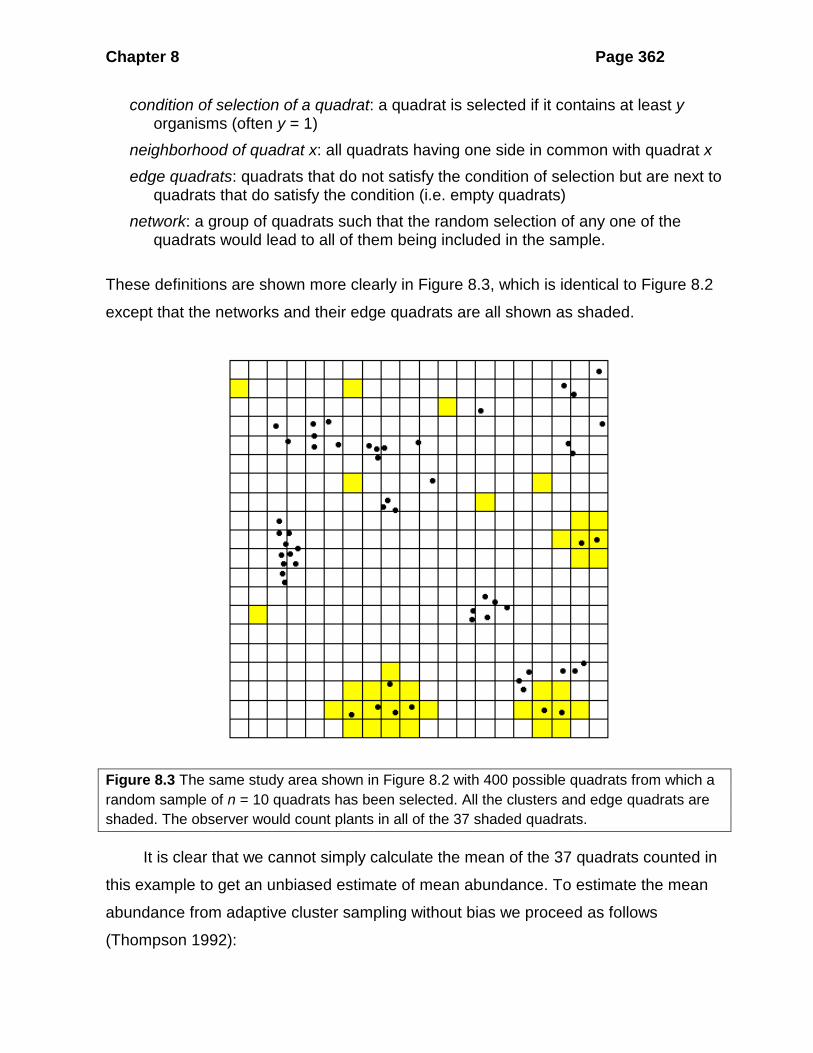
condition of selection of a quadrat: a quadrat is selected if it contains at least y organisms (often y = 1)
neighborhood of quadrat x: all quadrats having one side in common with quadrat x
edge quadrats: quadrats that do not satisfy the condition of selection but are next to quadrats that do satisfy the condition (i.e. empty quadrats)
network: a group of quadrats such that the random selection of any one of the quadrats would lead to all of them being included in the sample.
These definitions are shown more clearly in Figure 8.3, which is identical to Figure 8.2
except that the networks and their edge quadrats are all shown as shaded.
Figure 8.3 The same study area shown in Figure 8.2 with 400 possible quadrats from which a random sample of n = 10 quadrats has been selected. All the clusters and edge quadrats are shaded. The observer would count plants in all of the 37 shaded quadrats.
It is clear that we cannot simply calculate the mean of the 37 quadrats counted in
this example to get an unbiased estimate of mean abundance. To estimate the mean
abundance from adaptive cluster sampling without bias we proceed as follows
(Thompson 1992):

Chapter 8 Page 363
(1) Calculate the average abundance of each of the networks:
kk
ii
yw
m=∑
(8.36)
where wi = Average abundance of the i-th network yj = Abundance of the organism in each of the k-quadrats in the i-th network mi = Number of quadrats in the i-th network
(2) From these values we obtain an estimator of the mean abundance as follows:
ii
wx
n=∑
(8.37)
where x = Unbiased estimate of mean abundance from adaptive cluster sampling n = Number of initial sampling units selected via random sampling If the initial sample is selected with replacement, the variance of this mean is given by:
( )( )
( )
2
1ˆvar x1
n
ii
w x
n n=
−=
−
∑ (8.38)
where ( )ˆvar x = estimated variance of mean abundance for sampling with replacement and all other terms are defined above.
If the initial sample is selected without replacement, the variance of the mean is given
by:
( )( ) ( )
( )
2
1ˆvar x1
n
ii
N n w x
N n n=
− −=
−
∑ (8.39)
where N = total number of possible sample quadrats in the sampling universe
We can illustrate these calculations with the simple example shown in Figure 8.3.
From the initial random sample of n = 10 quadrats, three quadrats intersected networks
in the lower and right side of the study area. Two of these networks each have 2 plants
Chapter 8 Page 364
in them and one network has 5 plants. From these data we obtain from equation
(8.36):
2 2 5 0 07 8 15 1 1 0.08690 plants per quadrat
10
ii
wx
n
+ + + + + = = =
∑
Since we were sampling without replacement we use equation (8.39) to estimate the
variance of this mean:
( )( ) ( )
( )
( )
( )( )( )
2
1
2 2
ˆvar x12 2400 10 0.0869 0.08697 8
400 10 10 10.0019470
n
ii
N n w x
N n n=
− −=
− − − + − + =
−=
∑
We can obtain confidence limits from these estimates in the usual way:
( )ˆvarx t xα±
For this example with n = 10, for 95% confidence limits tα = 2.262 and the confidence
limits become:
( )( )0.0869 2.262 0.0019470 0.0869 0.0983± = ±
or from 0.0 to 0.185 plants per quadrat. The confidence limits extend below 0.0 but
since this is biologically impossible, the lower limit is set to 0. The wide confidence
limits reflect the small sample size in this hypothetical example.
When should one consider using adaptive sampling? Much depends on the
abundance and the spatial pattern of the animals or the plants being studied. In
general the more clustered the population and the rarer the organism, the more
efficient it will be to use adaptive cluster sampling. Thompson (1992) shows, for
example, from the data in Figure 8.2 that adaptive sampling is about 12% more
efficient than simple random sampling for n = 10 quadrats and nearly 50% more

Chapter 8 Page 365
efficient when n = 30 quadrats. In any particular situation it may well pay to conduct a
pilot experiment with simple random sampling and adaptive cluster sampling to
determine the size of the resulting variances.
8.3.2 Stratified Adaptive Cluster Sampling
The general principle of adaptive sampling can also be applied to situations that are
well enough studied to utilize stratified sampling. In stratified adaptive sampling random
samples are taken from each stratum in the usual way with the added condition that
whenever a sample quadrat satisfies some initial conditions (e.g. an animal is present),
additional quadrats from the neighborhood of that quadrat are added to the sample.
This type of sampling design would allow one to take advantage of the fact that a
population may be well stratified but clustered in each stratum in an unknown pattern.
Large gains in efficiency are possible if the organisms are clustered within each
stratum. Thompson (1992, Chap. 26) discusses the details of the estimation problem
for stratified adaptive cluster sampling. The conventional stratified sampling estimators
cannot be used for this adaptive design since the neighborhood samples are not
selected randomly.
8.4 SYSTEMATIC SAMPLING Ecologists often use systematic sampling in the field. For example, mouse traps may
be placed on a line or a square grid at 50 m intervals. Or the point-quarter distance
method might be applied along a compass line with 100 m between points. There are
many reasons why systematic sampling is used in practice, but the usual reasons are
simplicity of application in the field, and the desire to sample evenly across a whole
habitat.
The most common type of systematic sampling used in ecology is the centric
systematic area-sample illustrated in Figure 8.4. The study area is subdivided into
equal squares and a sampling unit is taken from the center of each square. The
samples along the outer edge are thus half the distance to the boundary as they are to
the nearest sample (Fig. 8.4). Note that once the number of samples has been
specified, there is only one centric sample for any area - all others would be eccentric
samples (Milne 1959).

Chapter 8 Page 366
Figure 8.4 Example of a study area subdivided into 20 equal-size squares with one sample taken at the center of each square. This is a centric systematic area-sample.
Statisticians have usually condemned systematic sampling in favor of random
sampling and have cataloged all the pitfalls that may accompany systematic sampling
(Cochran 1977). The most relevant problem for an ecologist is the possible existence
of periodic variation in the system under analysis. Figure 8.5 illustrates a hypothetical
example in which an environmental variable (soil water content, for example) varies in
a sine-wave over the study plot. If you are unlucky and happen to sample at the same
periodicity as the sine wave, you can obtain a biased estimate of the mean and the
variance (A in Fig. 8.5).
Obs
erve
d Va
lue
of X
Distance along transect line
A A AB
B
BB
BA AA
B

Chapter 8 Page 367
Figure 8.5 Hypothetical illustration of periodic variation in an ecological variable and the effects of using systematic sampling on estimating the mean of this variable. If you are unlucky and sample at A, you always get the same measurement and obtain a highly biased estimate of the mean. If you are lucky and sample at B, you get exactly the same mean and variance as if you had used random sampling. The important question is whether such periodic variation exists in the ecological world.
But what is the likelihood that these problems like periodic variation will occur in
actual field data? Milne (1959) attempted to answer this question by looking at
systematic samples taken on biological populations that had been completely
enumerated (so that the true mean and variance were known). He analyzed data from
50 populations and found that, in practice, there was no error introduced by assuming
that a centric systematic sample is a simple random sample, and using all the
appropriate formulae from random sampling theory.
Periodic variation like that in Figure 8.5 does not seem to occur in ecological
systems. Rather, most ecological patterns are highly clumped and irregular, so that in
practice the statistician's worry about periodic influences (Fig. 8.5) seems to be a
misplaced concern (Milne 1959). The practical recommendation is thus: you can use
systematic sampling but watch for possible periodic trends.
Caughley (1977) discusses the problems of using systematic sampling in aerial
surveys. He simulated a computer population of kangaroos, using some observed
aerial counts, and then sampled this computer population with several sampling
designs, as outlined in Chapter 4 (pp. 000-000). Table 8.5 summarizes the results
based on 20,000 replicate estimates done by a computer on the hypothetical kangaroo
population. All sampling designs provided equally good estimates of the mean
kangaroo density and all means were unbiased. But the standard error estimated from
systematic sampling was underestimated, compared with the true value. This bias
would reduce the size of the confidence belt in systematic samples, so that confidence
limits based on systematic sampling would not be valid because they would be too
narrow. The results of Caughley (1977) should not to be generalized to all aerial
surveys but they inject a note of warning into the planning of aerial counts if systematic
sampling is used.

Chapter 8 Page 368
TABLE 8.5 SIMULATED COMPUTER SAMPLING OF AERIAL TRANSECTS OF EQUAL LENGTH FOR A KANGAROO POPULATION IN NEW SOUTH WALESa
Sampling system
Method of analysis PPSb with replacement
Random with replacement
Random without
replacement
Systematic
Coefficient of variation 2% sampling rate (n = 10 transects)
9 9 9 9 20% sampling rate (n = 100 transects)
3 3 2 3
Bias in standard error (%) 2% sampling rate (n = 10 transects) 20% sampling rate (n = 100 transects)
0 0 0 -23 a Data from actual transects were used to set up the computer population, which was then sampled 20,000 times at two different levels of sampling. The percentage coefficient of variation of the population estimates and the relative bias of the calculated standard errors of the population estimates were compared for random and systematic sampling. b PPS, Probability-proportional-to-size sampling, discussed previously in Chapter 4. Source: Caughley, 1977b.
There is probably no issue on which field ecologists and statisticians differ more
than on the use of random vs. systematic sampling in field studies. If gradients across
the study area are important to recognize, systematic sampling like that shown in
Figure 8.4 will be more useful than random sampling to an ecologist. This decision will
be strongly affected by the exact ecological questions being studied. Some
combination of systematic and random sampling may be useful in practice and the
most important message for a field ecologist is to avoid haphazard or judgmental
sampling.
The general conclusion with regard to ecological variables is that systematic
sampling can often be applied, and the resulting data treated as random sampling
data, without bias. But there will always be a worry that periodic effects may influence
the estimates, so that if you have a choice of taking a random sample or a systematic

Chapter 8 Page 369
one, always choose random sampling. But if the cost and inconvenience of
randomization is too great, you may lose little by sampling in a systematic way.
8.5 MULTISTAGE SAMPLING Ecologists often subsample. For example, a plankton sample may be collected by
passing 100 liters of water through a net. This sample may contain thousands of
individual copepods or cladocerans and to avoid counting the whole sample, a
limnologist will count 1/100 or 1/1000 of the sample.
Statisticians describe subsampling in two ways. We can view the sampling unit in
this case to be the 100 liter sample of plankton and recognize that this sample unit can
be divided into many smaller samples, called subsamples or elements.
Figure 8.6 shows schematically how subsampling can be viewed. The technique
of subsampling has also been called two-stage sampling because the sample is taken
in two steps:
1. Select a sample of units (called the primary units) 2. Select a sample of elements within each unit.
Figure 8.6 Schematic illustration of two-stage sampling. In this example seven primary sampling units occur in the study area, and they contain different number of elements (from 4 to 49). For example, the 7 primary units could be 7 lakes of varying size and the elements could be benthic areas of 10 cm2. Alternatively they could be 7 woodlands varying in size from 4 to 49 ha. (• ) Sample elements selected for counting.

Chapter 8 Page 370
Many examples can be cited:
Type of data Primary sample unit Subsamples or Elements
Aphid infestation Sycamore tree Leaves within a tree
DDT contamination Clutch of eggs Individual eggs
Plankton 100-liter sample 1 ml subsample
Pollen profiles in peat 1 cm3 peat at given depth Microscope slides of pollen grains
Fish population in streams Entire stream
Habitat section of stream
If every primary sampling unit contains the same number of elements, subsampling is
relatively easy and straightforward (Cochran, 1977, Chapter 10). But in most ecological
situations, the primary sample units are of unequal size, and sampling is more
complex. For example, different sycamore trees will have different numbers of leaves.
It is important in ecological multistage sampling that the elements are of equal size–
only the primary sampling units can vary in size. For example, if you are surveying
different size woodlands, you should use a constant quadrat size in all of the
woodlands.
Clearly subsampling could be done at several levels and thus two-stage sampling
can be generalized to 3-stage sampling, and the general term multistage sampling is
used to describe any design in which there are two or more levels of sample selection
(Hankin 1984).
8.5.1 Sampling Units of Equal Size
Consider first the simplest case of multistage sampling in which n primary sample units
are picked and m subsamples are taken in each unit. For example, you might take 20
plankton samples (each of 100 liters of lake water) and from each of these 20 samples
count four subsamples (elements) of 1 ml each. We adopt this notation:
xij = measured value for the j element in primary unit i
xi = mean value per element in primary unit I = 1
mij
j
xm=
∑
The mean of the total sample is given by:
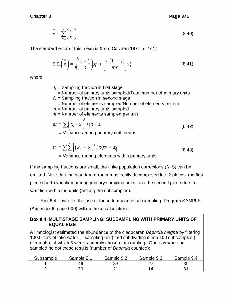
Chapter 8 Page 371
1 =
ni
i
xxn=
=
∑ (8.40)
The standard error of this mean is (from Cochran 1977 p. 277):
( )1 22 211 2
11S.E. = f ffx s s
n mn
= −− + (8.41)
where:
1
2
= Sampling fraction in first stage = Number of primary units sampled/Total number of primary units = Sampling fraction in second stage
= Number of elements sampled/Number of elements per unit
f
f
n = Number of primary units sampled = Number of elements sampled per unitm
( )2n
21 = / 1
= Variance among primary unit meansis x x n
= − −
∑ (8.42)
( )222 = / ( 1)
= Variance among elements within primary units
n m
ij is x x n m − − ∑∑ (8.43)
If the sampling fractions are small, the finite population corrections (f1, f2) can be
omitted. Note that the standard error can be easily decomposed into 2 pieces, the first
piece due to variation among primary sampling units, and the second piece due to
variation within the units (among the subsamples).
Box 8.4 illustrates the use of these formulae in subsampling. Program SAMPLE
(Appendix 6, page 000) will do these calculations.
Box 8.4 MULTISTAGE SAMPLING: SUBSAMPLING WITH PRIMARY UNITS OF EQUAL SIZE
A limnologist estimated the abundance of the cladoceran Daphnia magna by filtering 1000 liters of lake water (= sampling unit) and subdividing it into 100 subsamples (= elements), of which 3 were randomly chosen for counting. One day when he sampled he got these results (number of Daphnia counted):
Subsample Sample 9.1 Sample 9.2 Sample 9.3 Sample 9.4 1 46 33 27 39 2 30 21 14 31

Chapter 8 Page 372
3 42 56 65 45
Mean 39.33 36.67 35.33 38.33 In this example, n = 4 primary units sampled and N is very large (> 105) so the sampling fraction in the first stage (f1 ) is effectively 0.0. In the second stage m = 3 of a total of M = 100 possible elements, so the sampling fraction f2 is 0.03.
The mean number of Daphnia per 10 liters is given by equation (8.40):
139.33 36.67 35.33 38.33 + + + 37.42
4 4 4 4
ni
i
xxn
Daphnia=
= =
= =
∑
Note that this is the same as the mean that would be estimated if the entire data set were treated as a simple random sample. This would not be the case if the number of subsamples varied from primary sample unit to unit. The standard error of the estimated mean is from equation (8.41):
( ) ( )1 22 211 2
= 11S.E.f ffx s s
n mn−−
= +
First, calculate 2 21 2 and s s :
( ) ( )
2
2 221
2 2 222
(39.33 - 37.42) (36.67 - 37.42) + + 1 3 3
3.1368 (variance among primary unit means)46 39.33 (30 39.33)
( 1) 4(2) 4(2) 284.333 (variance among s
i
ij i
x xs
n
x xs
n m
= − = =
−=
− − −= = + +
− =
∑
∑∑
ubsamples)
It is clear from the original data that there is much more variation among the subsamples than there is among the primary samples. Since f1 is nearly zero, the second term disappears and
( )= 1S.E. = (3.1368) = 0.8856
4x
The 95% confidence interval would be ( tα = 2.20 for 11 d.f.):
( )=
S.E.37.42 2.20(0.8856)x t xα
=±
±

Chapter 8 Page 373
or from 35.5 to 39.4 Daphnia per 10 liters of lake water. If you wish to express these values in terms of the original sampling unit of 1000 liters, multiply them by 100 Program SAMPLE (Appendix 6) will do these calculations.
8.5.2 Sampling Units of Unequal Size
If the sampling units are of varying size, calculations of the estimated means and
variances are more complex. I will not attempt to summarize the specific details in this
book because they are too complex to be condensed simply (cf. Cochran 1977,
Chapter 11).
There are two basic choices that you must make in selecting a multistage
sampling design model - whether to chose the primary sampling units with equal
probability or with probability proportional to size (PPS). For example, in Figure 8.6 we
could choose two of the 7 primary sampling units at random, assigning probability of 1
in 7 to each. Alternatively, we could note that there are 123 elements in the study area
in Figure 8.6, and that the largest unit has 49 elements, so its probability of selection
should be 49/123 or 0.40, while the smallest unit has only 4 elements, so its probability
of selection should be 0.03.
It is usually more efficient to sample a population with some type of PPS sampling
design (Cochran 1977). But the problem is that, before you can use PPS sampling, you
must know (or have a good estimate of) all the numbers of elements in each of the
primary units in the population (the equivalent to the information in Figure 8.6). If you
do not know this, (as is often the case in ecology), you must revert to simple random
sampling or stratified sampling, or do a pilot study to get the required information.
Cochran (1977) shows that often there is little loss in precision by making a rough
estimate of the size of each primary unit, and using probability-proportional-to-
estimated-size (PPES) sampling.
Cochran (1977, Chapter 11) has a clear discussion of the various methods of
estimation that are applied to multistage sampling designs. Hankin (1984) discusses
the application of multistage sampling designs to fisheries research, and notes the
need for a computer to calculate estimates from the more complex models (Chao
1982). We have already applied a relatively simple form of PPS sampling to aerial

Chapter 8 Page 374
census (pp. 000-000). Ecologists with more complex multistage sampling designs
should consult a statistician. Program SAMPLE (Appendix 6, page 000) will do the
calculations in Cochran (1977, Chapter 11) for unequal size sampling units for equal
probability, PPS, or PPES sampling.
With multistage sampling you must choose the sample sizes to be taken at each
stage of sampling. How many sycamore trees should you choose as primary sampling
units? How many leaves should you sample from each tree? The usual
recommendation is to sample the same fraction of elements in each sampling unit,
since this will normally achieve a near-optimal estimate of the mean (Cochran 1977 p.
323). To choose the number of primary units to sample in comparison to the number of
elements to sample within units, you need to know the relative variances of the two
levels. For example, the total aphid population per sycamore tree may not be very
variable from tree to tree, but there may be great variability from leaf to leaf in aphid
numbers. If this is the case, you should sample relatively few trees and sample more
leaves per tree. Cochran (1977) should be consulted for the detailed formulae, which
depend somewhat on the relative costs of sampling more units compared with
sampling more elements. Schweigert and Sibert (1983) discuss the sample size
problem in multistage sampling of commercial fisheries. One useful rule-of-thumb is to
sample an average of m elements per primary sampling unit where:
222U
sms
≈ (8.44)
where:
( ) ( ) [ ]( )
22
2
2 2 21 2
Optimal number of elements to sample per primary unit Variance among elements within primary units
/ 1 as defined in equation (8.43)
/ = component of va
n mij i
U
ms
x x n m
s s s M
==
= − − = −
∑ ∑
( ) [ ]
21
2
1
riance among unit means Variance among primary units
/ 1 as defined in equation (8.41)n
ii
s
x x n=
== = − −
∑

Chapter 8 Page 375
For example, from the data in Box 8.4, 21s = 3.14 and 2
2s = 284.3 and M = 100 possible
subsamples per primary unit: thus -
2 284.3 = 3.14 - = 0.29100
284.3 = 31.3 elements0.29
Us
m
≈
There are 100 possible subsamples to be counted, and this result suggests you should
count 31 of the 100. This result reflects the large variance between subsample counts
in the data of Box 8.4.
Once you have an estimate of the optimal number of subsamples (m in equation
8.44) you can determine the sample size of the primary units (n) from knowing what
standard error you desire in the total mean x=
(equation 8.39) from the approximate
formula:
22 2 221 2 1
1 1 1S.E. = sx s s sn M mn N
= − + − (8.45)
where:
( )2122
=S.E. x Desired standard error of mean
Sample size of primary units needed Variance among primary units (equation 8.41) Variance among elements (equation 8.38) Total number of element
nssM
===== s per primary unit
Optimal number of elements to subsample (equation 8.43)m =
This equation can be solved for n if all the other parameters have been estimated in a
pilot survey or guessed from prior knowledge.
8.6 SUMMARY If you cannot count or measure the entire population, you must sample. Several types
of sampling designs can be used in ecology. The more complex the design, the more
efficient it is, but to use complex designs correctly you must already know a great deal
about your population.

Chapter 8 Page 376
Simple random sampling is the easiest and most common sampling design. Each
possible sample unit must have an equal chance of being selected to obtain a random
sample. All the formulas of statistics are based on random sampling, and probability
theory is the foundation of statistics. Thus you should always sample randomly when
you have a choice.
In some cases the statistical population is finite in size and the idea of a finite
population correction must be added into formulae for variances and standard errors.
These formulas are reviewed for measurements, ratios, and proportions.
Often a statistical population can be subdivided into homogeneous
subpopulations, and random sampling can be applied to each subpopulation
separately. This is stratified random sampling, and represents the single most powerful
sampling design that ecologists can adopt in the field with relative ease. Stratified
sampling is almost always more precise than simple random sampling, and every
ecologist should use it whenever possible.
Sample size allocation in stratified sampling can be determined using proportional
or optimal allocation. To use optimal allocation you need to have rough estimates of
the variances in each of the strata and the cost of sampling each strata. Optimal
allocation is more precise than proportional allocation, and is to be preferred.
Some simple rules are presented to allow you to estimate the optimal number of
strata you should define in setting up a program of stratified random sampling.
If organisms are rare and patchily distributed, you should consider using adaptive
cluster sampling to estimate abundance. When a randomly placed quadrat contains a
rare species, adaptive sampling adds quadrats in the vicinity of the original quadrat to
sample the potential cluster. This additional non-random sampling requires special
formulas to estimate abundance without bias.
Systematic sampling is easier to apply in the field than random sampling, but may
produce biased estimates of means and confidence limits if there are periodicities in
the data. In field ecology this is usually not the case, and systematic samples seem to
be the equivalent of random samples in many field situations. If a gradient exists in the

Chapter 8 Page 377
ecological community, systematic sampling will be better than random sampling for
describing it.
More complex multistage sampling designs involve sampling in two or more
stages, often called subsampling. If all the sample units are equal in size, calculations
are simple. But in many ecological situations the sampling units are not of equal size,
and the sampling design can become very complex so you should consult a
statistician. Multistage sampling requires considerable background information and
unless this is available, ecologists are usually better off using stratified random
sampling.
It is always useful to talk to a professional statistician about your sampling design
before you begin a large research project. Many sampling designs are available, and
pitfalls abound.
SELECTED REFERENCES Abrahamson, I.L., Nelson, C.R., and Affleck, D.L.R. 2011. Assessing the performance
of sampling designs for measuring the abundance of understory plants. Ecological Applications 21(2): 452-464.
Anganuzzi, A.A. & Buckland, S.T. 1993. Post-stratification as a bias reduction technique. Journal of Wildlife Management 57: 827-834.
Cochran, W.G. 1977. Sampling Techniques, 3rd ed. John Wiley and Sons, New York.
Legendre, P., Dale, M.R.T., Fortin, M.J., Gurevitch, J., Hohn, M., and Myers, D. 2002. The consequences of spatial structure for the design and analysis of ecological field surveys. Ecography 25(5): 601-615.
Milne, A. 1959. The centric systematic area-sample treated as a random sample. Biometrics 15: 270-297.
Morin, A. 1985. Variability of density estimates and the optimization of sampling programs for stream benthos. Canadian Journal of Fisheries and Aquatic Sciences 42: 1530-1534.Peterson, C.H., McDonald, L.L., Green, R.H., and
Erickson, W.P. 2001. Sampling design begets conclusions: the statistical basis for detection of injury to and recovery of shoreline communities after the 'Exxon Valdez¹ oil spill. Marine Ecology Progress Series 210: 255-283.
Thompson, S.K. 2012. Sampling. 3rd ed. John Wiley and Sons, Holboken, New Jersey.

Chapter 8 Page 378
Underwood, A.J., and Chapman, M.G. 2003. Power, precaution, Type II error and sampling design in assessment of environmental impacts. Journal of Experimental Marine Biology and Ecology 296(1): 49-70.
QUESTIONS AND PROBLEMS 8.1. Reverse the ratio calculations for the wolf-moose data in Box 8.2 (page 000) and
calculate the estimated ratio of moose to wolves for these data, along with the 95% confidence interval. Are these limits the reciprocal of those calculated in Box 8.2? Why or why not? (a) How would these estimates change if the population was considered infinite instead of finite?
8.2. Assume that the total volume of the lake in the example in Box 8.4 (page 000) is 1 million liters (N). Calculate the confidence limits that occur under this assumption and compare them with those in Box 8.4 which assumes N is infinite.
8.3. In the wood lemming (Myopus schisticolor) in Scandinavia there are two kinds of females - normal females that produce equal numbers of males and females, and special females that produce only female offspring. In a spruce forest with an estimated total population of 72 females, a geneticist found in a sample of 41 females, 15 individuals were female-only types. What is the estimate of the fraction of normal females in this population? What are the 95% confidence limits?
8.4. Hoisaeter and Matthiesen (1979) report the following data for the estimation of seaweed (Ulva) biomass for a reef flat in the Philippines: (quadrat size 0.25 m2)
Stratum Area (m2) Sample size Mean (g) Variance
I (near shore) 2175 9 0.5889 0.1661
II 3996 14 19.3857 179.1121
III 1590 7 2.1429 3.7962
IV
1039 6 0.2000 0.1120
Estimate the total Ulva biomass for the study zone, along with its 95% confidence limits. Calculate proportional and optimal allocations of samples for these data, assuming the cost of sampling is equal in all strata, and you require a confidence belt of ±25% of the mean.
8.5. Tabulate the observed no. of clams (x) in column 6 of Table 8.4 (page 000) in a cumulative frequency distribution. Estimate the optimal strata boundaries for this variable, based on 3 strata, using the cum f procedure. How do the results of

Chapter 8 Page 379
this stratification differ from those stratified on the depth variable (as in Table 8.4)?
8.6. A plant ecologist subsampled 0.25 m2 areas within 9 different deer-exclosures of 16 m2. She subsampled 2 areas within each exclosure, and randomly selected 9 of 18 exclosures that had been established in the study area. She got these results for herb biomass (g dry weight per 0.25 m2): Exclosure no.
Subsample 3 5 8 9 12 13 15 16 18
A 2 5 32 23 19 16 23 25 13
B 26 3 6 9 8 7 9 3 9
Estimate the mean biomass per 0.25 m2 for these exclosures, along with 95% confidence limits. How would the confidence limits for the mean be affected if you assumed all these estimates were replicates from simple random sampling with n = 18? What recommendation would you give regarding the optimal number of subsamples for these data?
8.7. Describe an ecological sampling situation in which you would not recommend using stratified random sampling. In what situation would you not recommend using adaptive cluster sampling?
8.8. How does multistage sampling differ from stratified random sampling?
8.9. Use the marked 25 x 25 grid on Figure 6.2 of the redwood seedlings (page 000) to set out an adaptive sampling program to estimate density of these seedlings. From a random number table select 15 of the possible 625 plots and apply adaptive cluster sampling to estimate density. Compare your results with simple random sampling of n = 15 quadrats.