chapter 7 the theory and estimation of production of production.pdf · the theory and estimation of...

Chapter 6Chapter 6The Theory and Estimation of

Production Managerial Economics: Economic

Tools for Today’s Decision Makers, 5/e By Paul Keat and Philip Young

2006 Prentice Hall Business Publishing Managerial Economics, 5/e Keat/Young

The Theory and Estimation of Production

• Chris Lim: VP Manufacturing.• What’s Bothering Him ???

• Key Factors: Marketing versus Manufacturing.

• Marketing/Production Differences ???• Up-Scale Niche Market versus Volume

Required for Low Costs.• Glass versus Cans and Plastics.


The Theory and Estimation of Production

• The Production Function• Short-Run Analysis

of Total, Average,

and Marginal Product• Long-Run Production Function• Estimation of Production Functions• Importance of Production Functions in

Managerial Decision Making


Learning Objectives

• Define production function and explain difference between short-run and long-run production function

• Explain “law of diminishing returns”

and how it relates to the Three Stages of Production

• Define the Three Stages of Production and explain why a rational firm always tries to operate in Stage II


Learning Objectives• Provide examples of types of inputs that might

go into a production function for a manufacturing or service company

• Describe various forms of a production function that are used in statistical estimation of these functions

• Briefly describe the Cobb-Douglas (Log Log) function and cite a few statistical studies that used this particular functional form in their analysis


The Production Function• Production function:

defines the relationship

between inputs and the maximum amount that can be produced within a given period of time with a given level of technology.

• Mathematically, the production function can be expressed as

Q=f(X1

, X2

, ..., Xk

)• Q: level of output• X1

, X2

, ..., Xk

: inputs used in the production process


The Production Function

• Key assumptions:• Some given “state of the art”

in the

production technology.• Whatever input or input combinations are

included in a particular function, the output resulting from their utilization is at the maximum level.• Technically Efficient Production.



• For simplicity we will often consider a production function of two inputs:

Q=f(X, Y)• Q: output• X: Labor (SR “proxy”)• Y: Capital (LR “proxy”)



• The short-run production function

shows the maximum quantity of good or service that can be produced by a set of inputs, assuming the amount of at least one of the inputs used remains unchanged.

• The long-run production function

shows the maximum quantity of good or service that can be produced by a set of inputs, assuming the firm is free to vary the amount of all the inputs being used.


Short-Run Analysis of Total, Average, and Marginal Product

• Alternative terms in reference to inputs• Inputs• Factors• Factors of production• Resources

• Alternative terms in reference to outputs• Output• Quantity (Q)• Total product (TP)• Product



• Marginal product (MP):

change in output (or Total Product) resulting from a unit change in a variable input.

Average Product (AP):

Total Product per unit of input used.

XQMPX Δ

Δ=

XQAP X =



8 37 60 83 96 107 117 127 1287 42 64 78 90 101 110 119 1206 37 52 64 73 82 90 97 1045 31 47 58 67 75 82 89 954 24 39 52 60 67 73 79 853 17 29 41 52 58 64 69 732 8 18 29 39 47 52 56 521 4 8 14 20 27 24 21 17

1 2 3 4 5 6 7 8

UN

ITS

OF

Y (K

= L

R)

Table 6.1: Soft Drink Bottling

UNITS OF X (L = SR)



X Q APP MPP1 8 8.0 --2 18 9.0 10.03 29 9.7 11.04 39 9.8 10.05 47 9.4 8.06 52 8.7 5.07 56 8.0 4.08 52 6.5 -4.0

Short Run Production Function (Y = K = 2 = FIXED)



• If MP > AP then AP is rising.

• If MP < AP then AP is falling.

• MP=AP when AP is maximized.• Show this

mathematically !!!• MAX AP F.O.C. !!!



SUMMARY OUTPUT CUBIC

Regression Statistics QUADMultiple R 1.000 0.996R Square 0.999 0.991Adjusted R Square 0.998 0.988Standard Error 0.732 1.957Observations 8 8

ANOVA

df SS MS FSignificance

FRegression 3 2,176 725.24 1,352 0.000Residual 4 2.15 0.54Total 7 2,178

CoefficientsStandard

Error t Stat P-value Lower 95%Upper 95%

Lower 99.0%

Upper 99.0%

Intercept -0.79 1.80 -0.44 68.57% -5.80 4.22 -9.09 7.52X 7.72 1.63 4.73 0.91% 3.19 12.25 0.20 15.24X SQ 1.22 0.41 2.98 4.09% 0.08 2.36 -0.67 3.10X CUBE -0.17 0.03 -5.63 0.49% -0.25 -0.09 -0.31 -0.03



PRODUCTION DATA

y = -0.1692x3 + 1.2186x2 + 7.7211x - 0.7857R2 = 0.999

y = -1.0655x2 + 16.435x - 9.1607R2 = 0.9912

-10

0

10

20

30

40

50

60

0 1 2 3 4 5 6 7 8 9

INPUTS (X)

QU

AN

TITY

QAPPMPPPoly. (Q)Poly. (Q)



PRODUCTION DATA

-6.0

-4.0

-2.0

0.0

2.0

4.0

6.0

8.0

10.0

12.0

0 1 2 3 4 5 6 7 8 9

INPUTS (X)

QU

AN

TITY

APPMPP

STAGE I STAGE I I STAGE III

MAX MPP !!!



• Law of Diminishing Returns:

As additional units of a variable input are combined with a fixed input, at some point the additional output (i.e., marginal product) starts to diminish.• Nothing says when diminishing returns will start

to take effect, only that it will happen at some point.

• All inputs added to the production process are exactly the same in individual productivity.

• Homogeneous Inputs.• MAY NOT be TRUE in “Real Life”

!!!



• The Three Stages of Production in the Short Run:• Stage I:

From zero units of the variable

input to where AP is maximized (where MP=AP)

• Stage II:

From the maximum AP to where MP=0

• Stage III:

From where MP ≤

0.


Three Stages of Production



• In the short run, rational firms should only be operating in Stage II.

• Why not Stage III?• Firm uses more variable inputs to produce less

output (can produce same with less

!!!).• Why not Stage I?

• Underutilizing fixed capacity: “not working to your potential”, “underachieving”

!!!

• Can increase output per unit by increasing the amount of the variable input (i.e., work harder

!!!)



• What level of input usage within Stage II is best for the firm?

• The answer depends upon how many units of output the firm can sell, the price of the product, and the monetary costs of employing the variable input.



• Profit = π

= P*Q –

PL

*L –

Pk

*K • where Q = f(L,K) = f(X,Y).• And ∂Q/∂L = MPL

, ∂Q/∂K = MPK

.• Profit MAX FOC w.r.t. (L,K):

• ∂π/∂L = P*∂Q/∂L –

PL

= 0.• ∂π/∂K = P*∂Q/∂K –

PK

= 0.• With K = Fixed (Short Run):

• P*MPL

= PL

or

MPL

= PL

/P or

P = PL

/MPL

.• Example: Cost or Ration/Price of Milk (or meat).



• Profit = π

= P*Q –

PL

*L –

Pk

*K • Profit MAX FOC w.r.t. (L,K):

• ∂π/∂L = P*∂Q/∂L –

PL

= 0.• With K = Fixed (Short Run):

• P*MPL

= PL

or

MPL

= PL

/P or

P = PL

/MPL

.• OR (Input):

MRL

= P*MPL

= MCL

= PL

• OR (Output):

MRQ

= P = MCQ

= PL

/MPL



• Profit = π

= P*Q –

PL

*L –

Pk


, ∂Q/∂K = MPK

.

• NOTE: MRQ

= ∂(P*Q)/∂Q = P.• NOTE: MCQ

= PL

/MPL = PK

/MPK

.• This demonstrates that MC = Inverse Function of MP

!!!



• Total Revenue Product (TRP):

market value of the firm’s output, computed by multiplying the total product by the market price.• TRP = Q · P

• Marginal Revenue Product (MRP):

change in the firm’s TRP resulting from a unit change in the number of inputs used.• MRP = = MP · PX

TRPΔΔ



• Total Labor Cost (TLC):

total cost of using the variable input, labor, computed by multiplying the wage rate by the number of variable inputs employed.• TLC = w · X

• Marginal Labor Cost (MLC):

change in total labor cost resulting from a unit change in the number of variable inputs used. Because the wage rate is assumed to be constant regardless of the number of inputs used, MLC is the same as the wage rate (w).



• Summary of relationship between demand for output and demand for input: SR• A profit-maximizing firm operating in perfectly

competitive output and input markets will be using the optimal amount of an input at the point at which the monetary value of the input’s marginal product is equal to the additional cost of using that input.

• MRP = MLC• MRL

= P*MPL

= WAGE = MCL



0 0 0 0 0 01 10,000 10,000 10,000 20,000 20,000 10,000 10,000 10,000 10,0002 25,000 12,500 15,000 50,000 30,000 20,000 10,000 30,000 20,0003 45,000 15,000 20,000 90,000 40,000 30,000 10,000 60,000 30,0004 60,000 15,000 15,000 120,000 30,000 40,000 10,000 80,000 20,0005 70,000 14,000 10,000 140,000 20,000 50,000 10,000 90,000 10,0006 75,000 12,500 5,000 150,000 10,000 60,000 10,000 90,000 07 78,000 11,143 3,000 156,000 6,000 70,000 10,000 86,000 -4,0008 80,000 10,000 2,000 160,000 4,000 80,000 10,000 80,000 -6,000

Product Price 2.00 Factor cost/unit 10000.00

TOTAL PROD.

TP

REVENUE PRODUCT AND LABOR COST

VAR. INPUT

X

Sample data have been entered as an example.

MAR. REV.

PROD. MRP

TOTAL REV.

PROD. TRP

MAR. PROD.

MP

AVE. PROD.

AP

MRP MINUS

MLC

TRP MINUS

TLC

MAR. LABOR COST MLC

TOTAL LABOR COST TLC



Optimum @ P =$2

Optimum @ P =$4

MRL = MCL



• Multiple variable inputs• Consider the relationship between the ratio of the

marginal product of one input and its cost to the ratio of the marginal product of the other input(s) and their cost.

• This is the EXPANSION PATH !!!• Other factors may outweigh this relationship

• Political/Economic risk factors.

k

k

wMP

wMP

wMP

==2

2

1

1



• Profit = π

= P*Q –

PL

*L –

Pk


, ∂Q/∂K = MPK

.• Profit MAX FOC w.r.t. (L,K):

• ∂π/∂L = P*∂Q/∂L –

PL

= 0 P = PL/MPL.• ∂π/∂K = P*∂Q/∂K –

PK

= 0 P = PK/MPK.• Rearranging/Combining these FOCs:

• P = PL

/MPL

= PK

/MPK

.• MPL

/MPK = PL

/PK

.• This is the EXPANSION PATH: Ratio of Optimal

Input Usage = f(Price

Ratios) !!!


Short-Run Analysis: Multiple InputsIsoquants !!!



8 37 60 83 96 107 117 127 1287 42 64 78 90 101 110 119 1206 37 52 64 73 82 90 97 1045 31 47 58 67 75 82 89 954 24 39 52 60 67 73 79 853 17 29 41 52 58 64 69 732 8 18 29 39 47 52 56 521 4 8 14 20 27 24 21 17

1 2 3 4 5 6 7 8

UN

ITS

OF

Y

UNITS OF X


Short-Run Analysis: Multiple Inputs



EXPANSION PATH:

PY /MPY =PX /MPX

PX /PY = MPX /MPY

Iso-Cost Function !!!



EXPANSION PATH:

PY /MPY =PX /MPX

PX /PY = MPX /MPY

Iso-Cost Functions !!!


The Long-Run Production Function

• In the long run, a firm has enough time to change the amount of all its inputs.• Effectively, all inputs are variable.

• The long run production process is described by the concept of returns to scale.



• If all

inputs into the production process are doubled, three things can happen:• output can more than double

• increasing returns to scale (IRTS).• output can exactly double

• constant returns to scale (CRTS).• output can less than double

• decreasing returns to scale (DRTS).


The Long-Run Production Function• One way to measure returns to scale is to use a

coefficient of output elasticity:

• If EQ

> 1 then IRTS.• If EQ

= 1 then CRTS.• If EQ

< 1 then DRTS.

inputsallinchangePercentageQinchangePercentage

=QE



Y X Q %Chg IP %Chg OP Scale ε Scale1 1 4 -- -- -- --2 2 18 100% 350% 3.5 IRTS3 3 41 50% 128% 2.6 IRTS4 4 60 33% 46% 1.4 IRTS5 5 75 25% 25% 1.0 CRTS6 6 90 20% 20% 1.0 CRTS7 7 119 17% 32% 1.9 IRTS8 8 128 14% 8% 0.5 DRTS



• Returns to scale can also be described using the following equation

hQ = f(kX, kY)

• If h > k then IRTS.• If h = k then CRTS.• If h < k then DRTS.


The Long-Run Production FunctionEXPANSION PATH:

PY /MPY =PX /MPX

PX /PY = MPX /MPY


Estimation of Production Functions• Forms of Production Functions

• Short run: existence of a fixed factor to which is added a variable factor

• One variable, one fixed factor.• Q = f(L)K

.• Increasing marginal returns followed by

decreasing marginal returns• Cubic function.• Q = a + bL

+ cL2

– dL3.• Diminishing marginal returns, but no Stage I

• Quadratic function.• Q = a + bL

-

cL2.


Forms of Production Functions


Estimation of Production Functions

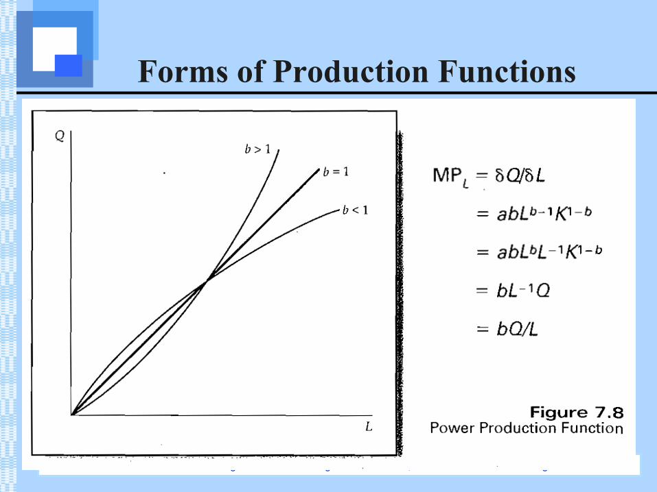
• Forms of Production Functions• Power function

• Q = aLbKc

• If b > 1, MP increasing• If b = 1, MP constant• If b < 1, MP decreasing• Can be transformed into a linear equation

when expressed in logarithmic terms• Ln(Q) = ln(a) + b*Ln(L)


Forms of Production Functions



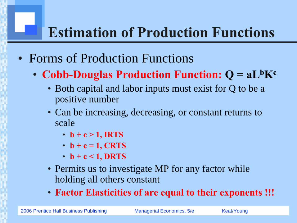
• Forms of Production Functions• Cobb-Douglas Production Function:

Q = aLbKc

• Both capital and labor inputs must exist for Q to be a positive number

• Can be increasing, decreasing, or constant returns to scale

• b + c > 1, IRTS• b + c = 1, CRTS• b + c < 1, DRTS

• Permits us to investigate MP for any factor while holding all others constant

• Factor Elasticities

of are equal to their exponents !!!


Production Functions: Cobb Douglas

Regression Statistics Q = aLbKc

Multiple R 0.990 ln(Q) = ln(a) + b*ln(L) + c*ln(K)R Square 0.981Adjusted R Square 0.979 0.986Standard Error 0.048Observations 20 a = exp(ln(Intercept)) = 15.136ANOVA

df SS MS F Significance FRegression 2 2.013 1.007 438.1 0.0%Residual 17 0.039 0.002Total 19 2.052

CoefficientsStandard

Errort Stat P-value Lower 95% Upper 95%

Intercept 2.717 0.221 12.29 0.0% 2.25 3.18lnL 0.664 0.075 8.81 0.0% 0.51 0.82lnK 0.321 0.147 2.19 4.3% 0.01 0.63

SUMMARY OUTPUT: Cobb-Douglas for Soft Drink Bottling (Table 7-6)

RTS: b+c =


Estimation of Production Functions1)

1a&2a:

1b&2b:

1c&2c: The expansion path: K = f(Pk, Pl, a, b c, L)

Q = a*(K^b)*(L^c)

The iso-quant equation: K = f(a, b c, Q, L).

The iso-cost equation: K = f(C, Pk, Pl, L).

P(l)/P(k) = MP(l)/MP(k) or P(l)/MP(l) = P(k)/MP(k) or MP(l)/P(l) = MP(k)/P(k)

K = C/P(k) - P(l)/P(k) * L

K = (Q/a)^(1/b)*L^(-c/b)

MP(l) = c*a*(K^b)*(L^(c-1))MP(l) = c*a*(K^b)*(L^c)*L^-1)

MP(k) = b*a*(K^(b-1)*(L^c)MP(k) = b*a*(K^b)*(K^-1)*(L^c)MP(k) = (b/K)*a*(K^b)*(L^c)MP(k) = (b/K)*Q

MP(l) = (c/L)*a*(K^b)*(L^c)MP(l) = (c/L)*Q

MP(l)/MP(k) = {(c/L)*Q}/{(b/K)*Q} = (c/b)*(K/L)

K = (b/c)*P(l)/P(k) * L



AAE421 Chapter 6 Bottling Data

0123456789

101112131415

0 2 4 6 8 10 12Labor

Kap

ital

Q = 60Q = 90Orig CostNew CostExp Path


Estimation of Production FunctionsCobb-Douglas Production Function

• Strengths:• Can be estimated by linear regression analysis.• Can accommodate any number of independent

variables.• Does not require that technology be held constant.

• Shortcomings:• Cannot show MP going through all three stages in

one specification.• Cannot show a firm or industry passing through

increasing, constant, and decreasing returns to scale.• Specification of data to be used in empirical

estimates.



• Statistical Estimation of Production Functions• Inputs should be measured as “flow”

rather than “stock”

variables, which is not always possible.

• Usually,

the most important input is labor.• Most difficult input variable is capital.• Must choose between

time series and

cross-sectional analysis.



• Aggregate Production Functions• Many studies using Cobb-Douglas did not deal

with individual firms, rather with aggregations of industries or an economy.

• Gathering data for aggregate functions can be difficult.

• For an economy: GDP could be used.• For an industry: data from Census of Manufactures

or production index from Federal Reserve Board.• For labor: data from Bureau of Labor Statistics.


Importance of Production Functions in Managerial Decision Making

• Production levels do not depend on how much a company wants to produce, but on how much its customers want to buy !!!

• Capacity Planning: planning the amount of fixed inputs that will be used along with the variable inputs. Good capacity planning requires:• Accurate forecasts

of demand.

• Effective communication

between the production and marketing functions.


Production Functions & Managerial Decision Making: Capacity Planning



Optimum @ MP1

Optimum @ MP2

MRL = MCL

chapter 7 the theory and estimation of production of production.pdf · the theory and estimation of...

Documents