chapter 7 periodicity - smithcallahan/cic/ch7.pdf · 7.1 periodic behavior example 1: populations....
TRANSCRIPT

DVI file created at 9:40, 28 January 2008Copyright 1994, 2008 Five Colleges, Inc.
Chapter 7
Periodicity
In seeking to describe and understand natural processes, we search for pat-terns. Patterns that repeat are particularly useful, because we can predictwhat they will do in the future. The sun rises every day and the seasons Many patterns
are periodicrepeat every year. These are the most obvious examples of cyclic, or peri-odic, patterns, but there are many more of scientific interest, too. Periodicbehavior is the subject of this chapter. We shall take up the questions of de-scribing and measuring it. To begin, let’s look at some intriguing examplesof periodic or near-periodic behavior.
7.1 Periodic Behavior
Example 1: Populations. In chapter 4 we studied several models thatdescribe how interacting populations might change over time. Two of thosemodels—one devised by May and the other by Lotka and Volterra—predictthat when one species preys on another, both predator and prey populationswill fluctuate periodically over time. How can we tell if that actually happensin nature? Ecologists have examined data for a number of species. Some of Predator and
prey populationsfluctuate periodically
the best evidence is found in the records of Hudson’s Bay Company, whichtrapped fur-bearing animals in Canada for almost 200 years. The graph onthe next page gives the data for the numbers of lynx pelts harvested in theMackenzie River region of Canada during the years 1821 to 1934 (Finerty,1980). (The lynx is a predator; its main prey is the snowshoe hare.) Clearlythe numbers go up and down every 10 years in something like a periodicpattern. There is even a more complex pattern, with one large bulge and
419

DVI file created at 9:40, 28 January 2008Copyright 1994, 2008 Five Colleges, Inc.
420 CHAPTER 7. PERIODICITY
three smaller ones, that repeats about every 40 years. Data sets like thisappear frequently in scientific inquiries, and they raise important questions.Here is one: If a quantity we are studying really does fluctuate in a periodicway, why might that happen? Here is another: If there appear to be severalperiodic influences, what are they, and how strong are they? To explorethese questions we will develop a language to describe and analyze periodicfunctions.
1820 1840 1860 1880 1900 1920
2000
4000
6000
year
Annual harvest of lynx pelts
pelts
Example 2: The earth’s orbit. The earth orbits the sun, returning to itsThe position and theshape of the earth’sorbit both fluctuateperiodically
original position after one year. This is the most obvious periodic behavior; itexplains the cycle of seasons, for example. But there are other, more subtle,periodicities in the earth’s orbital motion. The orbit is an ellipse which turnsslowly in space, returning to its original position after about 23,000 years.This movement is called precession. The orbit fluctuates in other ways thathave periods of 41,000 years (the obliquity cycle) and 95,000, 123,000, and413,000 years (the eccentricity cycles).
Example 3: The climate. In 1941 the Serbian geophysicist Milutin Mi-lankovitch proposed that all the different periodicities in the earth’s orbitFluctuations in the
climate appear in thegeological record
affect the climate—that is, the long-term weather patterns over the entireplanet. Therefore, he concluded, there should also be periodic fluctuations inthe climate, with the same periods as the earth’s orbit. In fact, it is possibleto test this hypothesis, because there are features of the geological recordthat tell us about long-term weather patterns. For example, in a year whenthe weather is warm and wet, rains will fill streams and rivers with mud thatis eventually carried to lake bottoms. The result is a thick sediment layer. In

DVI file created at 9:40, 28 January 2008Copyright 1994, 2008 Five Colleges, Inc.
7.1. PERIODIC BEHAVIOR 421
a dry year, the sediment layer will be thinner. Over geological time, lakes dryout and their beds turn to clay or shale. By measuring the annual layers overthousands of years, we can see how the climate has varied. Other featuresthat have been analyzed the same way are the thickness of annual ice layersin the Antarctic ice cap, the fluctuations of CO2 concentrations in the icecaps, changes in the O18/O16 ratio in deep-sea sediments and ice caps. Inchapter 12 we will look at the results of one such study.
1820 1840 1860 1880 1900 1920
25
50
75
100
125
year
Daily average number of sunspots
suns
pots
Example 4: Sunspot cycles. The number of sunspots fluctuates, reachinga peak every 11 years or so. The graph above shows the average daily numberof sunspots during each year from 1821 to 1934. Compare this with the lynxgraph which covers the same years. Some earthbound events (e.g., auroras,television interference) seem to follow the same 11-year pattern. Accordingto some scientists, other meteorological phenomena—such as rainfall, averagetemperature, and CO2 concentrations in the atmosphere—are also “sunspotcycles,” fluctuating with the same 11-year period. It is difficult to get firm Data can have
both periodic andrandom influences
evidence, though, because many fluctuations with different possible causescan be found in the data. Even if there is an 11-year cycle, it may be“drowned out” by the effects of these other causes.
The problem of detecting periodic fluctuations in “noisy” data is onethat scientists often face. In chapter 12 we will introduce a mathematicaltool called the power spectrum, and we will use it to detect and measureperiodic behavior—even when it is swamped by random fluctuations.

DVI file created at 9:40, 28 January 2008Copyright 1994, 2008 Five Colleges, Inc.
422 CHAPTER 7. PERIODICITY
7.2 Period, Frequency, and
the Circular Functions
We are familiar with the notions of period and frequency from everydayexperience. For example, a full moon occurs every 28 days, which meansthat a lunar cycle has a period of 28 days and a frequency of once per 28days. Moreover, whatever phase the moon is in today, it will be in the samephase 28 days from now. Let’s see how to extend these notions to functions.
The function y = g(x) whose graph is sketched below has a patternDefining aperiodic function that repeats. The space T between one high point and the next tells us the
period of this repeating pattern. There is nothing special about the highpoint, though. If we take any two points x and x + T that are spaced oneperiod apart, we find that g has the same value at those point.
x x + T
g(x) g(x + T)
x
y
y = g(x)
T
(This is analogous to saying that the moon is in the same phase on any twodays that are 28 days apart.) The condition g(x + T ) = g(x) for every xguarantees that g will be periodic. We make it the basis of our definition.
Definition. We say that a function g(x) is periodic
if there is a positive or negative number T for which
g(x + T ) = g(x) for all x.
We call T a period of g(x).

DVI file created at 9:40, 28 January 2008Copyright 1994, 2008 Five Colleges, Inc.
7.2. PERIOD, FREQUENCY, AND THE CIRCULAR FUNCTIONS 423
Since the graph of g repeats after x increases by T , it also repeats after A periodic functionhas many periods. . .x increases by 2T , or −3T , or any integer multiple (positive or negative) of
T . This means that a periodic function always has many periods. (That’swhy the definition refers to “a period” rather than “the period.”) The sameis true of the moon; its phases also repeat after 2× 28 days, or 3× 28, days. . . . but we call the
smallest positive onethe period
Nevertheless, we think of 28 days as the period of the lunar cycle, because wesee the entire pattern precisely once. We can say the same for any periodicfunction:
Definition. The period of a periodic function is itssmallest positive period. It is the size of a single cycle.
Another measure of a periodic function is its frequency. Consider first the Frequency
lunar cycle. Its frequency is the number of cycles—or fractions of a cycle—that occur in unit time. If we measure time in days, then the frequency is1/28-th of a cycle per day. If we measure time in years, though, then thefrequency is about 13 cycles per year. Here is the calculation:
365 days/year
28 days/cycle≈ 13 cycles/year.
Using this example as a pattern, we make the following definition.
Definition. If the function g(x) is periodic, then itsfrequency is the number of cycles per unit x.
Notice that the period and the frequency of the lunar cycle are reciprocals: The frequency ofa cycle is the
reciprocal of its periodthe period is 28 days—the time needed to complete one cycle—while thefrequency is 1/28-th of a cycle per day. In the example below, t is measuredin seconds and g has a period of .2 seconds. Its frequency is therefore 5 cyclesper second.
0 1 2 3
secondst
yy = g(t)
Period: .2 seconds per cycle Frequency: 5 cycles per second
.2 seconds

DVI file created at 9:40, 28 January 2008Copyright 1994, 2008 Five Colleges, Inc.
424 CHAPTER 7. PERIODICITY
In general, if f is the frequency of a periodic function g(x) and T is itsperiod, then we have
f =1
Tand T =
1
f.
The units are also related in a reciprocal fashion: if the period is measuredin seconds, then the frequency is measured in cycles per second.
Because many quantities fluctuate periodically over time, the input vari-able of a periodic function will often be time. If time is measured in seconds,The units for
measuring frequencyover time
then frequency is measured in “cycles per second.” The term Hertz is aspecial unit used to measure time frequencies; it equals one cycle per sec-ond. Hertz is abbreviated Hz; thus a kilohertz (kHz) and a megahertz
(MHz) are 1,000 and 1,000,000 cycles per second, respectively. This unit iscommonly used to describe sound, light, radio, and television waves. Forexample, an orchestra tunes to an A at 440 Hz. If an FM radio stationbroadcasts at 88.5 MHz, this means its carrier frequency is 88,500,000 cyclesper second.
Quantities may also be periodic in other dimensions. For instance, ascientist studying the phenomenon of ripple formation in a river bed mightFunctions can be
periodic over otherunits as well
be interested in the function h(x) measuring the height of a ripple as afunction of its distance x along the river bed. This would lead to a functionof period, say, 10 inches and corresponding frequency of .1 cycle per inch.
x
yt
(cos t , sin t )
1
Circular functions. While there are innumerableexamples of periodic functions, two in particular areconsidered basic: the sine and the cosine. They are calledcircular functions because they are defined by means of acircle. To be specific, take the circle of radius 1 centeredat the origin in the x, y-plane. Given any real number t,measure a distance of t units around the circumferenceof the circle. Start on the positive x-axis, and measure
counterclockwise if t is positive, clockwise if t is negative. The coordinatesof the point you reach this way are, by definition, the cosine and the sinefunctions of t, respectively:
x = cos(t),
y = sin(t).

DVI file created at 9:40, 28 January 2008Copyright 1994, 2008 Five Colleges, Inc.
7.2. PERIOD, FREQUENCY, AND THE CIRCULAR FUNCTIONS 425
The whole circumference of the circle measures 2π units. Therefore, if we Why cos t and sin t
are periodicadd 2π units to the t units we have already measured, we will arrive backat the same point on the circle. That is, we get to the same point on thecircle by measuring either t or t + 2π units around the circumference. Wecan describe the coordinates of this point two ways:
(cos(t), sin(t)) or (cos(t + 2π), sin(t + 2π)).
Thuscos(t + 2π) = cos(t) sin(t + 2π) = sin(t),
so cos(t) and sin(t) are both periodic, and they have the same period, 2π.Here are their graphs. By reading their slopes we can see (sin t)′ = cos t and(cos t)′ = − sin t.
t
xx = cos( t)
−π π 2π 3π 4π−1
1
t
yy = sin( t)
−π π2π
3π4π
−1
1
t
1
The circular functions are constructed without reference to angles; the Radian measure
variable t is measured around the circumference of a circle (of radius 1).Nevertheless, we can think of t as measuring an angle, as shown at the right.In this case, t is called the radian measure of the angle. The units are verydifferent from the degree measurement of an angle: an angle of 1 radian ismuch larger than an angle of 1 degree. The radian measure of a 90◦ angle isπ/2 ≈ 1.57, for instance. If we thought of t as an angle measured in degrees,the slope of sin(t) would equal .017 cos t! (See the exercises.) Only when wemeasure t in radians do we get a simple result: (sin t)′ = cos t. This is whywe always measure angles in radians in calculus.
Compare the graph of y = sin(t) above with that of y = sin(4t), below. Changing thefrequency
t
yy = sin(4t)
−π π 2π 3π 4π−1
1

DVI file created at 9:40, 28 January 2008Copyright 1994, 2008 Five Colleges, Inc.
426 CHAPTER 7. PERIODICITY
Their scales are identical, so it is clear that the frequency of sin(4t) is fourtimes the frequency of sin(t). The general pattern is described in the followingtable.
function period frequency
sin(t) cos(t) 2π 1/2πsin(4t) cos(4t) 2π/4 4/2πsin(bt) cos(bt) 2π/b b/2π
Notice that it is the frequency—not the period—that is increased by a factorof b when we multiply the input variable by b.
By using the information in the table, we can construct circular functionsConstructing acircular function witha given frequency
with any period or frequency whatsoever. For instance, suppose we wanteda cosine function x = cos(bt) with a frequency of 5 cycles per unit t. Thismeans
5 = frequency =b
2π,
which implies that we should set b = 10π and x = cos(10πt). In order to seethe high-frequency behavior of this function better, we magnify the graph abit. In the figure below, you can compare the graphs of x = cos(10πt) andx = cos(t) directly. We still have equal scales on the horizontal and verticalaxes. Finally, notice that cos(10πt) has exactly 5 cycles on the interval0 ≤ t ≤ 1.
t
x
x = cos(10πt)
x = cos(t)
1 2
−1
1

DVI file created at 9:40, 28 January 2008Copyright 1994, 2008 Five Colleges, Inc.
7.2. PERIOD, FREQUENCY, AND THE CIRCULAR FUNCTIONS 427
We will denote the frequency by ω, the lower case letter omega from the Frequency ω
Greek alphabet. If
ω = frequency =b
2π,
then b = 2πω. Therefore, the basic circular functions of frequency ω arecos(2πωt) and sin(2πωt).
Suppose we take the basic sine function sin(2πωt) of frequency ω and Amplitude
multiply it by a factor A:
y = A sin(2πωt).
The graph of this function oscillates between y = −A and y = +A. Thenumber A is called the amplitude of the function.
t
yy = Asin(2πωt)
amplitude
−1/ω 1/ω 2/ω 3/ω
−A
A
The sine function of amplitude A and frequency ω
Physical interpretations. Sounds are transmitted to our ears as fluctu-ations in air pressure. Light is transmitted to our eyes as fluctuations in amore abstract medium—the electromagnetic field. Both kinds of fluctuationscan be described using circular functions of time t. The amplitude and thefrequency of these functions have the physical interpretations given in thefollowing table.
frequencyamplitude frequency range
sound loudness pitch 10–15000 Hz
light intensity color 4 × 10¹⁴ – 7.5 × 10¹⁴ Hz

DVI file created at 9:40, 28 January 2008Copyright 1994, 2008 Five Colleges, Inc.
428 CHAPTER 7. PERIODICITY
Exercises
Circular functions
1. Choose ω so that the function cos(2πωt) has each of the following periods.
a) 1 b) 5 c) 2π d) π e) 1/3
2. Determine the period and the frequency of the following functions.
a) sin(x), sin(2x), sin(x) + sin(2x)
b) sin(2x), sin(3x), sin(2x) + sin(3x)
c) sin(6x), sin(9x), sin(6x) + sin(9x)
3. Suppose a and b are positive integers. Describe how the periods ofsin(ax), sin(bx), sin(ax) + sin(bx) are related. (As the previous exerciseshows, the relation between the periods depends on the relation between aand b. Make this clear in your explanation.)
4. a) What are the amplitude and frequency of g(x) = 5 cos(3x)?
b) What are the amplitude and frequency of g′(x)?
5. a) Is the antiderivative
∫
x
0
5 cos(3t) dt periodic?
b) If so, what are its amplitude and frequency?
6. Use the definition of the circular functions to explain why
sin(−t) = − sin(t), sin(π
2− t
)
= cos(t),
cos(−t) = + cos(t), sin(π − t) = sin(t),
hold for all values of t. Describe how these properties are reflected in thegraphs of the sine and cosine functions.
7. a) What is the average value of the function sin(s) over the interval0 ≤ s ≤ π? (This is a half-period.)
b) What is the average value of sin(s) over π/2 ≤ s ≤ 3π/2? (This is also ahalf-period.)
c) What is the average value of sin(s) over 0 ≤ s ≤ 2π? (This is a fullperiod.)

DVI file created at 9:40, 28 January 2008Copyright 1994, 2008 Five Colleges, Inc.
7.2. PERIOD, FREQUENCY, AND THE CIRCULAR FUNCTIONS 429
d) Let c be any number. Find the average value of sin(s) over the full periodc ≤ s ≤ c + 2π.
e) Your work should demonstrate that the average value of sin(s) over a fullperiod does not depend on the point c where you begin the period. Does it?Is the same true for the average value over a half period? Explain.
8. a) What is the period T of P (t) = A sin(bt)?
b) Let c be any number. Find the average value of P (t) over the full periodc ≤ t ≤ c + T . Does this value depend on the choice of c?
c) What is the average value of P (t) over the half-period 0 ≤ t ≤ T/2?
Phase
There is still another aspect of circular functions to consider besides am-plitude and frequency. It is called phase difference. We can illustrate thiswith the two functions graphed below. They have the same amplitude andfrequency, but differ in phase.
t
y
y = Asin(bt − ϕ)
y = Asin(bt )
ϕ/b
ϕ/b : phase shift
Specifically, the variable u in the expression sin(u) is called the phase. Inthe dotted graph the phase is u = bt, while in the solid graph it is u = bt−ϕ.They differ in phase by bt − (bt − ϕ) = ϕ. In the exercises you will see whya phase difference of ϕ produces a shift—which we call a phase shift—ofϕ/b in the graphs. (ϕ is the Greek letter phi.)
9. The functions sin(x) and cos(x) have the same amplitude and frequency;they differ only in phase. In other words,
cos(x) = sin(x − ϕ)

DVI file created at 9:40, 28 January 2008Copyright 1994, 2008 Five Colleges, Inc.
430 CHAPTER 7. PERIODICITY
for an appropriately chosen phase difference ϕ. What is the value of ϕ?
10. The functions sin(x) and − sin(x) also differ only in phase. What istheir phase difference? In other words, find ϕ so that
sin(x − ϕ) = − sin(x).
[Note: A circular function and its negative are sometimes said to be “180degrees out of phase.” The value of ϕ you found here should explain thisphrase.]
11. What is the phase difference between sin(x) and − cos(x)?
12. a) Graph y = sin(t) and y = sin(t − π/3) on the same plane.
b) What is the phase difference between these two functions?
c) What is the phase shift between their graphs?
13. a) Graph together on the same coordinate plane y = cos(t) and y =cos(t + π/4).
b) What is the phase difference between these two functions?
c) What is the phase shift between their graphs?
14. We know y = cos(t) has a maximum at the origin. Determine thepoint closest to the origin where y = cos(t + π/4) has its maximum. Is thesecond maximum shifted from the first by the amount of the phase shift youidentified in the previous question?
15. Repeat the last two exercises for the pair of functions y = cos(2t) andcos(2t + π/4). Is the phase difference equal to the phase shift in this case?
16. Verify that the graph of y = A sin(bt−ϕ) crosses the t-axis at the pointt = ϕ/b. This shows that A sin(bt−ϕ) is “phase-shifted” by the amount ϕ/bin relation to A sin(bt). (Refer to the graph on page 429.)
17. a) At what point nearest the origin does the function A cos(bt − ϕ)reach its maximum value?
b) Explain why this shows A cos(bt − ϕ) is “phase-shifted” by the amountϕ/b in relation to A cos(bt).

DVI file created at 9:40, 28 January 2008Copyright 1994, 2008 Five Colleges, Inc.
7.2. PERIOD, FREQUENCY, AND THE CIRCULAR FUNCTIONS 431
18. a) Let f(x) = sin(x) − .7 cos(x). Using a graphing utility, sketch thegraph of f(x).
b) The function f(x) is periodic. What is its period? From your graph,estimate its amplitude.
c) In fact, f(x) can be viewed as a “phase-shifted” sine function:
f(x) = A sin(bx − ϕ).
From your graph, estimate the phase difference ϕ and the amplitude A.
19. a) For each of the values ϕ = 0, π/4, π/2, 3π/4, π, sketch the graphy = sin(x) · sin(x − ϕ) over the interval 0 ≤ x ≤ 2π. Put the five graphs onthe same coordinate plane.
b) For which graphs is the average value positive, for which is it negative,and for which is it 0? Estimate by eye.
20. The purpose of this exercise is to determine the average value
F (ϕ) =1
2π
∫
2π
0
sin(x) sin(x − ϕ) dx
for an arbitrary value of the parameter ϕ. To stress that the average valueis actually a function of ϕ, we have written it as F (ϕ). Here is one wayto determine a formula for F (ϕ) in terms of ϕ. First, using a “sum of twoangles” formula and exercise 6, above, write
sin(x − ϕ) = cos(ϕ) sin(x) − sin(ϕ) cos(x)
Then consider
1
2π
[
cos(ϕ)
∫
2π
0
(sin(x))2dx − sin(ϕ)
∫
2π
0
sin(x) cos(x) dx
]
,
and determine the values of the two integrals separately.
21. a) Sketch the graph of the average value function F (ϕ) you found inthe previous exercise. Use the interval 0 ≤ ϕ ≤ π.
b) In exercise 19 you estimated the value of F (ϕ) for five specific values ofϕ. Compare your estimates with the exact values that you can now calculateusing the formula for F (ϕ).

DVI file created at 9:40, 28 January 2008Copyright 1994, 2008 Five Colleges, Inc.
432 CHAPTER 7. PERIODICITY
22. Sketch the graph of y = cos(x) sin(x−ϕ) for each of the following valuesof ϕ: 0, π/2, 2π/3, π. Use the interval 0 ≤ x ≤ 2π. Estimate by eye theaverage value of each function over that interval.
23. a) Obtain a formula for the average value function
G(ϕ) =1
2π
∫
2π
0
cos(x) sin(x − ϕ) dx.
and sketch the graph of G(ϕ) over the interval 0 ≤ ϕ ≤ π.
b) Use your formula for G(ϕ) to compute the average value of the functioncos(x) sin(x−ϕ) exactly for ϕ = 0, π/2, 2π/3, π. Compare these values withyour estimates in the previous exercise.
24. How large a phase difference ϕ is needed to make the graphs of y =sin(3x) and y = sin(3x − ϕ) coincide?
25. Sketch the graphs of the following functions.
a) y = 3 sin(2x − π/6) − 1
b) y = 4 sin(2x − π) + 2.
c) y = 4 sin(2x + π) + 2.
26. The function whose graph is sketchedat the right has the form
G(x) = A sin(bx − ϕ) + C.
Determine the values of A, b, C, and ϕ.t
y y = Asin(bt - ϕ) + c
−2
5
−2 2 4 6
27. Write equations for three different functions that all have amplitude 4,period 5, and whose graphs pass through the point (6, 7). Be sure the func-tions are really different—if g(t) is one solution, then h(t) = g(t + 5) wouldreally be just the same solution.
Derivatives with degrees
28. a) In this exercise measure the angle θ in degrees. Estimate the deriva-tive of sin(θ) at θ = 0◦ by calculating sin(θ)/θ for θ = 2◦, 1◦, .5◦.

DVI file created at 9:40, 28 January 2008Copyright 1994, 2008 Five Colleges, Inc.
7.3. DIFFERENTIAL EQUATIONS WITH PERIODIC SOLUTIONS 433
b) Estimate the derivative of sin(θ) at θ = 60◦ in a similar way. Is (sin(30◦))′ =cos(30◦)?
29. a) Your calculations in the previous exercise should support the claimthat (sin(θ))′ = k cos(θ) for a particular value of k, when θ is measured indegrees. What is k, approximately?
b) If t is the radian measure of an angle, and if θ is its degree measure, thenθ will be a function of t. What is it? Now use the chain rule to get a preciseexpression for the constant k.
7.3 Differential Equations with Periodic Solutions
The models of predator–prey interactions constructed by Lotka–Volterra andMay (see chapter 4) provide us with examples of systems of differential equa-tions that have periodic solutions. Similar examples can be found in manyareas of science. We shall analyze some of them in this section. In particu-lar, we will try to understand how the frequency and the amplitude of theperiodic solutions depend on the parameters given in the model.
Oscillating Springs
We want to study the motion of a weight that hangs from the endof a spring. First let the weight come to rest. Then pull down onit. You can feel the spring pulling it back up. If you push up onthe weight, the spring (and gravity) push it back down. The forceyou feel is called the spring force. Now release the weight; it will
m x
cm
0restposition
move. We’ll assume that the only influence on the motion is the spring force.(In particular, we will ignore the force of friction.) With this assumption wecan construct a model to describe the motion. We’ll suppose the weight hasa mass of m grams, and it is x centimeters above its rest position after tseconds. (If the weight goes below the rest position, then x will be negative.)
The linear spring
The simplest assumption we can reasonably make is that the spring force is A linear spring
proportional to the amount x that the spring has been displaced:
force = −c x.

DVI file created at 9:40, 28 January 2008Copyright 1994, 2008 Five Colleges, Inc.
434 CHAPTER 7. PERIODICITY
In this case the spring is said to be linear. The multiplier c is called thespring constant. It is a positive number that varies from one spring toanother. The minus sign tells us the force pushes down if x > 0, and it pushesup if x < 0. Because this model describes an oscillating spring governed bya linear spring force, it is called the linear oscillator.
To see how the spring force affects the motion of the weight, we useNewton’s laws ofmotion Newton’s laws. In their simplest form, they say that the force acting on a
body is the product of its mass and its acceleration. Suppose v = dx/dt isthe velocity of the weight in cm/sec, and dv/dt is its acceleration in cm/sec2.Then
force = mdv
dtgm-cm/sec2.
If we equate our two expressions for the force, we get
mdv
dt= −c x or
dv
dt= −b2x cm/sec2,
where we have set c/m = b2. It is more convenient to write c/m as b2 here,because then b =
√
c/m itself will be measured in units of 1/sec. (To seewhy, note that −b2x is measured in units of cm/sec2.)
Suppose we move the weight to the point x = a cm on the scale, hold it
The linear oscillator motionless for a moment, and then release it at time t = 0 sec. This gives usthe initial value problem
x′ = v, x(0) = a,
v′ = −b2x, v(0) = 0.
If we give the parameters a and b specific values, we can solve this initialThe solution withfixed parameters value problem using Euler’s method. The figure below shows the solution
x(t) for two different sets of parameter values:
a = 4 cm, a = −5 cm,
b = 5 per sec, b = 9 per sec.
t
x
sec
cma = −5 cmb = 9 /sec
a = 4 cmb = 5 /sec−5
4
1 2 3

DVI file created at 9:40, 28 January 2008Copyright 1994, 2008 Five Colleges, Inc.
7.3. DIFFERENTIAL EQUATIONS WITH PERIODIC SOLUTIONS 435
The graphs were made in the usual way, with the differential equation solverof a computer. They indicate that the weight bounces up and down in aperiodic fashion. The amplitude of the oscillation is precisely a, and thefrequency appears to be linked directly to the value of b. For instance, whenb = 9 /sec, the motion completes just under 3 cycles in 2 seconds. This is afrequency of slightly less than 1.5 cycles per second. When b = 5 /sec, themotion undergoes roughly 2 cycles in 2.5 seconds, a frequency of about .8cycles per second. If the frequency is indeed proportional to b, the multipliermust be about 1/6:
frequency ≈ b
6cycles/sec.
We can get a better idea how the parameters in a problem affect the solu- The solutionfor arbitrary
parameter valuestion if we solve the problem with a method that doesn’t require us to fix thevalues of the parameters in advance. This point is discussed in chapter 4.2,pages 214–218. It is particularly useful if we can express the solution by aformula, which it turns out we can do in this case. To get a formula, let usbegin by noticing that
(x′)′ = v′ = −b2x.
In other words, x(t) is a function whose second derivative is the negative ofitself (times the constant b2). This suggests that we try
x(t) = sin(bt) or x(t) = cos(bt).
You should check that x′′ = −b2x in both cases.Turn now to the initial conditions. Since sin(0) = 0, there is no way to
modify sin(bt) to make it satisfy the condition x(0) = a. However,
x(t) = a cos(bt)
does satisfy it. Finally, we can use the differential equation x′ = v to definev(t):
v(t) = (a cos(bt))′ = −ab sin(bt).
Notice that v(0) = −ab sin(0) = 0, so the second initial condition is satisfied.In summary, we have a formula for the solution that incorporates the The formula proves the
motion is periodicparameters. With this formula we see that the motion is really periodic—afact that Euler’s method could only suggest. Furthermore, the parametersdetermine the amplitude and frequency of the solution in the following way:
position : a cos(bt) cm from rest after t secamplitude : a cmfrequency : b/2π cycles/sec

DVI file created at 9:40, 28 January 2008Copyright 1994, 2008 Five Colleges, Inc.
436 CHAPTER 7. PERIODICITY
We can see the relation between the motion and the parameters in the graphbelow (in which we take a > 0).
Graph of the generallinear oscillator
t
x
sec
cm
a x = acos(bt )
2π/b 4π/b 6π/b
Here are some further properties of the motion that follow from our for-mula for the solution. Recall that the parameter b depends on the mass mof the weight and the spring constant c: b2 = c/m.
• The amplitude depends only on the initial conditions, not on the massm or the spring constant c.
• The frequency depends only on the mass and the spring constant, noton the initial amplitude.
These properties are a consequence of the fact that the spring force is linear.As we shall see, a non-linear spring and a pendulum move differently.
The non-linear spring
The harder you pull on a spring, the more it stretches. If the stretchis exactly proportional to the pull (i.e., the force), the spring is linear.
x
forcenon-linear
(hard) spring
linearspring
force = −cx
linearrange
In other words, to double the stretch you mustdouble the force. Most springs behave this waywhen they are stretched only a small amount.This is called their linear range. Outside thatrange, the relation is more complicated. One pos-sibility is that, to double the stretch, you mustincrease the force by more than double. A springthat works this way is called a hard spring. Thegraph at the left shows the relation between theapplied force and the displacement (or stretch x)of a hard spring.

DVI file created at 9:40, 28 January 2008Copyright 1994, 2008 Five Colleges, Inc.
7.3. DIFFERENTIAL EQUATIONS WITH PERIODIC SOLUTIONS 437
In a nonlinear spring, force is no longer proportional to displacement.Thus, if we write
force = −c x
we must allow the multiplier c to depend on x. One simple way to achievethis is to replace c by c + γx2. (We use x2 rather than just x to ensure that−x will have the same effect as +x. The multiplier γ is the Greek lettergamma.) Then
force = −c x − γx3.
Since force = m dv/dt as well, we have
mdv
dt= −c x − γx3 or
dv
dt= −b2x − βx3 cm/sec2.
Here b2 = c/m and β = γ/m. By taking the same initial conditions as before,we get the following initial value problem:
A non-linear oscillatorx′ = v, x(0) = a,
v′ = −b2x − βx3, v(0) = 0.
To solve this problem using Euler’s method, we must fix the values of thethree parameters. For the two parameters that determine the spring force,we choose:
b = 5 per sec β = .2 per cm2-sec2.
We have deliberately chosen b to have the same value it did for our firstsolution to the linear problem. In this way, we can compare the non-linear Comparing a hard
spring to a linear springspring to the linear spring that has the same spring constant. We do this inthe figure below. The dashed graph shows the linear spring when its initialamplitude is a = 4 cm. The solid graph shows the hard spring when itsinitial amplitude is a = 1.5 cm. Note that the two oscillations have the samefrequency.
t
x
sec
cm
1.5
4
1 2 3hard spring
linear spring

DVI file created at 9:40, 28 January 2008Copyright 1994, 2008 Five Colleges, Inc.
438 CHAPTER 7. PERIODICITY
The non-linear spring behaves like the linear one because the amplitudesThe effect of amplitudeon acceleration are small. To understand this reason, we must compare the accelerations
of the two springs. For the linear spring we have v′ = −25x, while forthe non-linear spring, v′ = −25x − .2x3. As the following graph shows,these expressions are approximately equal when the amplitude x lies between+2 cm and −2 cm. In other words, the linear range of the hard spring is
x
cm
v′cmsec2
linear: = −25x
non-linear: = −25x − .2x3
−8 −4 4 8
200
−200
−2 ≤ x ≤ 2 cm. Since the initial amplitude was 1.5 cm—well within thelinear range—the hard spring acts like a linear one. In particular, its fre-quency is approximated closely by the formula b/2π cycles per second. Thisis 5/2π ≈ .8 Hz.
A different set of circumstances is reflected in the following graph. TheLarge-amplitudeoscillations hard spring has been given an initial amplitude of 8 cm. As the graph of
v′ shown above indicates, the hard spring experiences an acceleration about50% greater than the linear spring at the that amplitude.
t
x
sec
cm
4
8
1 2 3
linear spring ≈ 21/2 cycles
hard spring ≈ 3 cycles

DVI file created at 9:40, 28 January 2008Copyright 1994, 2008 Five Colleges, Inc.
7.3. DIFFERENTIAL EQUATIONS WITH PERIODIC SOLUTIONS 439
As a consequence, the hard spring oscillates with a noticeably higher fre- The frequency of anon-linear spring
depends onits amplitude
quency! It completes 3 cycles in the time it takes the linear spring to com-plete 21
2—or 6 cycles while the linear spring completes 5. The frequency of
the hard spring is therefore about 6/5-th the frequency of the linear spring,or 6/5 × 5/2π = 3/π ≈ .95 Hz.
The solutions of the non-linear spring problem still look like cosine func-tions, but they’re not. It’s easier to see the difference if we take a largeamplitude solution, and look at velocity instead of position. In the graphbelow you can see how the velocity of a hard spring differs from a pure sine A mathematical
commentfunction of the same period and amplitude. Since there are no sine or cosinefunctions here, we can’t even yet be sure that the motion of a non-linearspring is truly periodic! We will prove this, though, in the next section byusing the notion of a first integral.
time
velocity
sec
cmsec
pure sine functionvelocity of hard spring
There are other ways we might have modified the basic equation v′ = Other non-linearsprings−b2x to make the spring non-linear. The formula v′ = −b2x − βx3 is only
one possibility. Incidentally, our study of a hard spring was based on choosingβ > 0 in this formula. Suppose we choose β < 0 instead. As you will seein the exercises, this is a soft spring: we can double the stretch in a softspring by using less than double the force. The pendulum, which we willstudy next, behaves like a soft spring.
Although we can use sine and cosine functions to solve the linear oscillatorproblem, there are, in general, no formulas for the solutions to the non-linearoscillator problems. We must use numerical methods to find their graphs—aswe have done in the last three pages.
The basic differential equation for a linear spring is also used to model avibrating string. Think of a tightly-stretched wire, like a piano string or a The harmonic oscillator
guitar string. Let x be the distance the center of the string has moved from

DVI file created at 9:40, 28 January 2008Copyright 1994, 2008 Five Colleges, Inc.
440 CHAPTER 7. PERIODICITY
rest at any instant t. The larger x is, the more strongly the tension on thestring will pull it back towards its rest position. Since x is usually very small,it makes sense to assume that this “restoring force” is a linear function of x:−c x. If v is the velocity of the string, then mv′ = −c x by Newton’s laws ofmotion. Because of the connection between vibrating strings and music, thisdifferential equation is called the harmonic oscillator.
The Sine and Cosine Revisited
The sine and cosine functions first appear in trigonometry, where they aredefined for the acute angles of a right triangle. Negative angles and angleslarger than 90◦, are outside their domain. This is a serious limitation. Toovercome it, we redefine the sine and cosine on a circle. The main conse-quence of this change is that the sine and cosine become periodic.
However, neither circles nor triangles are particularly useful if we wantA computabledefinition of thesine and cosine
to calculate the values of the sine or the cosine. (How would you use one ofthem to determine sin(1) to four—or even two—decimal places accuracy?)Our experience with the harmonic oscillator gives yet another way to definethe sine and the cosine functions—a way that conveys computational power.
The idea is simple. With hindsight we know that u = sin(t) and v = cos(t)are the solutions to the initial value problem
u′ = v, u(0) = 0,
v′ = −u v(0) = 1.
Now make a fresh start with this initial value problem, and define u = sin(t)and v = cos(t) to be its solution! Then we can calculate sin(1), for instance,by Euler’s method. Here is the result.
number estimate ofof steps sin(1)
1001 000
10 000100 000
1 000 000
.845671
.841892
.841513
.841475
.841471
So we can say sin(1) = .8415 to four decimal places accuracy.

DVI file created at 9:40, 28 January 2008Copyright 1994, 2008 Five Colleges, Inc.
7.3. DIFFERENTIAL EQUATIONS WITH PERIODIC SOLUTIONS 441
Our point of view here is that differential equations define functions. Inchapter 10, we shall consider still another method for defining and calculatingthese important functions, using infinite series.
The Pendulum
x
v
0
1
We are going to study the motion of a pendulum that can swing in a full 360◦
circle. To keep the physical details as simple as possible, we’ll assume its massis 1 unit, and that all the mass is concentrated in the center of the pendulumbob, 1 unit from the pivot point. Assume that the pendulum is x units fromits rest position at time t, where x is measured around the circular paththat the bob traces out. Assume the velocity is v. Take counterclockwisepositions and velocities to be positive, clockwise ones to be negative. Whenthe pendulum is at rest we have x = v = 0.
x
xG
F
G sinx = F
When the pendulum is moving, there must be forces at work. Let’s ignorefriction, as we did with the spring. The force that pulls the pendulum backtoward the rest position is gravity. However, gravity itself—G in the figureat the right—pulls straight down. Part of the pull of G works straight alongthe arm of the pendulum, and is resisted by the pivot. (If not, the pendulumwould be pulled out of the pivot and fall to the floor!) It is the other part,labelled F, that moves the pendulum sideways.
The size of F depends on the position x of the pendulum. When x = 0,the sideways force F is zero. When x = π/2 (the pendulum is horizontal),the entire pull of G is “sideways”, so F = G. To see how F depends on xin general, note first that we can think of x as the radian measure of theangle between the pendulum and the vertical (because x is measured arounda circle of radius 1). In the small right triangle, the hypotenuse is G andthe side opposite the angle x is exactly as long as F. By trigonometry, F =G sin x.
Let’s choose units which make the size of G equal to 1. Then the size Newton’s lawsproduce a modelof the pendulum
of F is simply sin x. Since F points in the clockwise (or negative) directionwhen x is positive, we must write F = − sin x. According to Newton’s lawsof motion, the force F is the product of the mass and the acceleration of thependulum. Since the mass is 1 unit and the acceleration is v′ = x′′, we finallyget x′′ = − sin x, or
x′ = v v′ = − sin x.

DVI file created at 9:40, 28 January 2008Copyright 1994, 2008 Five Colleges, Inc.
442 CHAPTER 7. PERIODICITY
Now that we have an explicit description of the restoring force, we canThe pendulum isa soft spring see that the pendulum behaves like a non-linear spring. However, it is true
that doubling the displacement x always less than doubles the force, as thegraph below demonstrates. Thus the pendulum is like a soft spring.
x
v′
1 2 3−1−2−3
a linear spring
the penduluma soft spring
v′ = −sin x
v′ = −x
Because a swinging pendulum is used keep time, it is important to controlthe period of the swing. Physics analyzes how the period depends on thependulum’s length and mass. We will confine ourselves to analyzing how theperiod depends on its amplitude.
Let’s draw on our experience with springs. According to the graph above,Small-amplitudeoscillations the restoring force of the pendulum is essentially linear for small amplitudes—
say, for −.5 ≤ x ≤ .5 radians. Therefore, if the amplitude stays small, it isreasonable to expect that the pendulum will behave like a linear oscillator.As the graph indicates, the differential equation of the linear oscillator isv′ = −x. This is of the form v′ = −b2x with b = 1. The period of sucha linear oscillator is 2π/b = 2π ≈ 6.28. Let’s see if the pendulum has thisperiod when it swings with a small amplitude. We use Euler’s method tosolve the initial value problem
x′ = v, x(0) = a,
v′ = − sin x, v(0) = 0,
for several small values of a. The results appear in the graph below.
t
x
6 12−.4
.2
.5
As you can see, small amplitude oscillations have virtually the same period.Thus, we would not expect the fluctuations in the amplitude of the pendulumon a grandfather’s clock to affect the timekeeping.

DVI file created at 9:40, 28 January 2008Copyright 1994, 2008 Five Colleges, Inc.
7.3. DIFFERENTIAL EQUATIONS WITH PERIODIC SOLUTIONS 443
What happens to the period, though, if the pendulum swings in a large Large-amplitudeoscillationsarc? The largest possible initial amplitude we can give the pendulum would
point it straight up. The pendulum is then 180◦ from the rest position,corresponding to a value of x = π = 3.14159 . . .. In the graph below wesee the solution that has an initial amplitude of x = 3, which is very nearthe maximum possible. Its period is much larger than the period of thesolution with x = .5, which has been carried over from the previous graph forcomparison. Even the solution with x = 2 has a period which is significantlylarger that the solution with x = .5.
t
x
3 6 9 12
.5
2
3
x = .5
x = 2
x = 3
We saw that the period of a hard spring got shorter (its frequency increased)when its amplitude increased. But the pendulum is a soft spring and showsmotions of longer period as its initial amplitude is increased. Notice howflat the large-amplitude graph is. This means that the pendulum lingersat the top of its swing for a long time. That’s why the period becomes solarge. Check the graph now and confirm that the period of the large swingis about 17.
DVI file created at 9:40, 28 January 2008Copyright 1994, 2008 Five Colleges, Inc.
444 CHAPTER 7. PERIODICITY
Although we can’t get formulas to describe the motion of the pendulumThe pendulum at rest
for most initial conditions, there are two special circumstances when we can.Consider a pendulum that is initially at rest: x = 0 and v = 0 when t = 0.It will remain at rest forever: x(t) = 0, v(t) = 0 for all t ≥ 0. What we reallymean is that the constant functions x(t) = 0 and v(t) = 0 solve the initialvalue problem
x′ = v, x(0) = 0,
v′ = − sin x, v(0) = 0.
There is another way for the pendulum to remain at rest. The key is thatThe pendulumbalanced on end v must not change. But v′ = − sin x, so v will remain fixed if v′ = − sin x = 0.
Now, sin x = 0 if x = 0. This yields the rest solution we have just identified.But sin x is also zero if x = π. You should check that the constant functionsx(t) = π, v(t) = 0 solve this initial value problem:
x′ = v, x(0) = π,
v′ = − sin x, v(0) = 0.
Since the pendulum points straight up when x = π radians, this motionlesssolution corresponds to the pendulum balancing on its end.
These two solutions are called equilibrium solutions (from the LatinStable and unstableequilibrium solutions æqui-, equal + libra, a balance scale). If the pendulum is disturbed from its
rest position, it tends to return to rest. For this reason, rest is said to bea stable equilibrium. Contrast what happens if the pendulum is disturbedwhen it is balanced upright. This is said to be an unstable equilibrium. Wewill take a longer look at equilibria in chapter 8.
Predator–Prey Ecology
Many animal populations undergo nearly periodic fluctuations in size. It isWhy do populationsfluctuate? even more remarkable that the period of those fluctuations varies little from
species to species. This fascinates ecologists and frustrates many who hunt,fish, and trap those populations to make their livelihood. Why should therebe fluctuations, and can something be done to alter or eliminate them?
There are models of predator-prey interaction that exhibit periodic be-havior. Consequently, some researchers have proposed that the fluctuationsobserved in a real population occur because that species is either the preda-tor or the prey for another species. The models themselves have differentproperties; we will study one proposed by R. May. As we did with the spring

DVI file created at 9:40, 28 January 2008Copyright 1994, 2008 Five Colleges, Inc.
7.3. DIFFERENTIAL EQUATIONS WITH PERIODIC SOLUTIONS 445
and the pendulum, we will ask how the frequency and amplitude of periodicsolutions depend on the initial conditions.
May’s model involves two populations that vary in size over time: thepredator y and the prey x. The numbers x and y have been set to anarbitrary scale; they lie between 0 and 20. The model also has six adjustableparameters, but we will simply fix their values:
prey: x′ = .6 x(
1 − x
10
)
− .5 xy
x + 1,
predator: y′ = .1 y(
1 − y
2x
)
.
These equations will be our starting point. However, if you wish to learnmore about the premises behind May’s model, you can refer to chapter 4.1(page 191).
To begin to explore the model, let’s see what happens to the prey popu- A predator-freeequilibrium . . .lation when there are no predators (y = 0). Then the size of x is governed by
the simpler differential equation x′ = .6x(1 − x/10). This is logistic growth,and x will eventually approach the carrying capacity of the environment,which in this case is 10. (See chapter 4.1, pages 183–185.) In fact, youshould check that
x(t) = 10, y(t) = 0,
is an equilibrium solution of May’s original differential equations. Now sup-pose we introduce a small number of predators: y = .1. Then the equilibrium . . . upset by predators
is lost, and the predator and prey populations fall into cyclic patterns withthe same period:
t
x, y
10
.10 50 100 150 200
x: prey
y: predator
period ≈ 39

DVI file created at 9:40, 28 January 2008Copyright 1994, 2008 Five Colleges, Inc.
446 CHAPTER 7. PERIODICITY
In the other models of periodic behavior we have studied, the frequencySolutions with variousinitial conditions . . . and amplitude have depended on the initial conditions. Is the same true
here? The following graphs illustrate what happens if the initial populationsare either
x = 8, y = 2, or x = 1.1, y = 2.2.
For the sake of comparison, the solution with x = 10, y = .1 is also carriedover from the previous page.
t
x, y
8
2
0 50 100 150 200
x: prey
y: predator
t
x, y
1.12.2
0 50 100 150 200
x: prey
y: predator
t
x, y
10
.10 50 100 150 200
x: prey
y: predator
In all of these graphs, periodic behavior eventually emerges. What ismost striking, though, is that it is the same behavior in all cases. The. . . all have the
same amplitudeand frequency
amplitude and the period do not depend on the initial conditions. Moreover,even though the populations peak at different times on the three graphs (i.e.,the phases are different), the y peak always comes about 14 time units afterthe x peak.

DVI file created at 9:40, 28 January 2008Copyright 1994, 2008 Five Colleges, Inc.
7.3. DIFFERENTIAL EQUATIONS WITH PERIODIC SOLUTIONS 447
Proving a Solution Is Periodic
The graphs in the last ten pages provide strong evidence that non-linear Can we prove thatsystems have periodic
oscillations?springs, pendulums, and predator-prey systems can oscillate in a periodicway. The evidence is numerical, though. It is based on Euler’s method,which gives us only approximate solutions to differential equations. Can wenow go one step further and prove that the solutions to these and othersystems are periodic?
Notice that we already have a proof in the case of a linear spring. Thesolutions are given by formulas that involve sines and cosines, and these are The virtue
of a formulaperiodic by their very design as circular functions. But we have no formulasfor the solutions of the other systems. In particular, we are not able to sayanything about the general properties of the solutions (the way we can aboutsine and cosine functions). The approach we take now does not depend onhaving a formula for the solution.
It may seem that what we should do is develop more methods for finding formulas for solutions.In fact, two hundred years of research was devoted to this goal, and much has been accomplished.However, it is now clear that most solutions simply have no representation “in closed form” (thatis, as formulas). This isn’t a confession that we can’t find the solutions. It just means theformulas we have are inadequate to describe the the solutions we can find.
The pendulum—a qualitative approach
x = a
v = 0
Stage 1:
Let’s work with the pendulum and model it by the following initial valueproblem:
x′ = v, x(0) = a,
v′ = − sin x, v(0) = 0.
We’ll assume 0 < a < π. Thus, at the start the pendulum is motionless andraised to the right. Call this stage 1. We’ll analyze what happens to x andv in a qualitative sense. That is, we’ll pay attention to the signs of thesequantities, and whether they’re increasing or decreasing, but not their exactnumerical values.
x = 0
v = −V1
Stage 2:
According to the differential equations, v determines the rate at which xchanges, and x determines the rate at which v changes. In particular, sincewe start with 0 < x < π, the expression − sin x must be negative. Thus v′ isnegative, so v decreases, becoming more and more negative as time goes on.Consequently, x changes at an ever increasing negative rate, and eventually
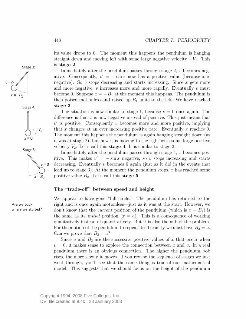
DVI file created at 9:40, 28 January 2008Copyright 1994, 2008 Five Colleges, Inc.
448 CHAPTER 7. PERIODICITY
its value drops to 0. The moment this happens the pendulum is hangingstraight down and moving left with some large negative velocity −V1. Thisis stage 2.
Immediately after the pendulum passes through stage 2, x becomes neg-ative. Consequently, v′ = − sin x now has a positive value (because x isnegative). So v stops decreasing and starts increasing. Since x gets moreand more negative, v increases more and more rapidly. Eventually v mustbecome 0. Suppose x = −B1 at the moment this happens. The pendulum isthen poised motionless and raised up B1 units to the left. We have reachedstage 3.
x = −B1
v = 0
Stage 3:
x = 0
v = V2
Stage 4:
x = B2
v = 0
Stage 5:
The situation is now similar to stage 1, because v = 0 once again. Thedifference is that x is now negative instead of positive. This just means thatv′ is positive. Consequently v becomes more and more positive, implyingthat x changes at an ever increasing positive rate. Eventually x reaches 0.The moment this happens the pendulum is again hanging straight down (asit was at stage 2), but now it is moving to the right with some large positivevelocity V2. Let’s call this stage 4. It is similar to stage 2.
Immediately after the pendulum passes through stage 4, x becomes pos-itive. This makes v′ = − sin x negative, so v stops increasing and startsdecreasing. Eventually v becomes 0 again (just as it did in the events thatlead up to stage 3). At the moment the pendulum stops, x has reached somepositive value B2. Let’s call this stage 5.
The “trade-off” between speed and height
We appear to have gone “full circle.” The pendulum has returned to theright and is once again motionless—just as it was at the start. However, weAre we back
where we started? don’t know that the current position of the pendulum (which is x = B2) isthe same as its initial position (x = a). This is a consequence of workingqualitatively instead of quantitatively. But it is also the nub of the problem.For the motion of the pendulum to repeat itself exactly we must have B2 = a.Can we prove that B2 = a?
Since a and B2 are the successive positive values of x that occur whenv = 0, it makes sense to explore the connection between x and v. In a realpendulum there is an obvious connection. The higher the pendulum bobrises, the more slowly it moves. If you review the sequence of stages we justwent through, you’ll see that the same thing is true of our mathematicalmodel. This suggests that we should focus on the height of the pendulum

DVI file created at 9:40, 28 January 2008Copyright 1994, 2008 Five Colleges, Inc.
7.3. DIFFERENTIAL EQUATIONS WITH PERIODIC SOLUTIONS 449
bob and the magnitude of the velocity. This is called the speed; it is justthe absolute value |v| of the velocity.
x 11
cos x
h
A little trigonometry shows us that when the pendu-lum makes an angle of x radians with the vertical, theheight of the pendulum bob is
h = 1 − cos x.
When x is a function of time t, then h is too and we have
h(t) = 1 − cos(x(t)).
Our intuition about the pendulum tells us that every change in heightis offset by a change in speed. (This is the “trade-off.”) It makes sense,therefore, to compare the rates at which the height and the speed changeover time. However, the speed |v(t)| involves an absolute value, and this Changes in speed
. . . modifiedis difficult to deal with in calculus. (The absolute value function is notdifferentiable at 0.) Since we are using |v| simply as a way to ignore thedifference between positive and negative velocities, we can replace |v| by v2.Then we find
d
dt(v(t))2 = 2 · v(t) · v′(t) = −2 · v · sin x.
Notice that we needed the chain rule to differentiate (v(t))2. After that weused the differential equations of the pendulum to replace v′ by − sin x.
The height of the pendulum changes at this rate: Changes in height
d
dth(t) = sin(x(t)) · x′(t) = sin x · v.
We needed the chain rule again, and we used the differential equations of thependulum to replace x′ by v.
The two derivatives are almost exactly the same; except for sign, theydiffer only by a factor 2. If we use 1
2v2 instead of v2, then the trade-off is
exact: every increase in 1
2v2 is exactly matched by a decrease in h, and vice
versa. Therefore, if we combine 1
2v2 and h to make the new quantity
E = 1
2v2 + h = 1
2v2 + 1 − cos x,
then we can say that the value of E does not change as the pendulum moves.Since E depends on v and h, and these are functions of the time t, E Showing E is a
constantitself is a function of t. To say that E doesn’t change as the pendulum movesis to say that this function is a constant—in other words, that its derivative

DVI file created at 9:40, 28 January 2008Copyright 1994, 2008 Five Colleges, Inc.
450 CHAPTER 7. PERIODICITY
is 0. This was, in fact, the way we constructed E in the first place. Let’sremind ourselves of why this worked. Since E = 1
2v2 + h,
dE
dt= v · v′ + h′ = v · (− sin x) + sin x · v = 0.
To get the second line we used the fact that v′ = − sin x and x′ = v whenx(t) and v(t) describe pendulum motion.
The quantity E is called the energy of the pendulum. The fact that Edoesn’t change is called the conservation of energy of the pendulum. Anumber of problems in physics can be analyzed starting from the fact thatthe energy of many systems is constant.
Let’s calculate the value of E at the five different stages of our pendulum:
stage v x h E
1 0 a 1 − cos a 1 − cos a2 −V1 0 0 1
2(−V1)
2
3 0 −B1 1 − cos B1 1 − cos B1
4 V2 0 0 1
2V2
2
5 0 B2 1 − cos B2 1 − cos B2
By the conservation of energy, all the quantities in the right-hand columnhave the same value. Looking at the value for E in stages 2 and 4, we see thatV1 = V2—whenever the pendulum is at the bottom of its swing (x = 0), it ismoving with the same speed, the velocity being positive when the pendulumis swinging to the right, negative when it is swinging to the left. Similarly,if we look at the value of E at stages 1, 3, and 5, we see that
1 − cos a = 1 − cos B1 = 1 − cos B2.
We can put this another way: whenever the pendulum is motionless, it mustbe back at its starting height h = 1 − cos a.
In particular, we have thus shown that B2 (the position of the pendulumafter it’s gone over and back) = a (the position of the pendulum at the be-ginning). Thus the value for x and the value for v are the same in stage 5 andin stage 1—the two stages are mathematically indistinguishable. Since the. . . and that the
oscillations are periodic solution to an initial value problem depends only on the differential equationand the initial values, what happens after stage 5 must be identical to whathappens after stage 1—the second swing of the pendulum must be identicalto the first! Thus the motion is periodic, which completes our proof.

DVI file created at 9:40, 28 January 2008Copyright 1994, 2008 Five Colleges, Inc.
7.3. DIFFERENTIAL EQUATIONS WITH PERIODIC SOLUTIONS 451
You can also use the fact that the value of E doesn’t change to determinethe velocities −V1 and V2 that the pendulum achieves at the bottom of itsswing. In the exercises you are asked to show that
V1 = V2 =√
2 − 2 cos a.
First Integrals
Notice in what we have just done that we haven’t solved the differentialequation for the pendulum in the sense of finding explicit formulas giving xand v in terms of t. Instead we found a combination of x and v that remainedconstant over time and used this to deduce some of the behavior of x and v.Such a combination of the variables that remains constant is called a first First integrals
integral of the differential equation. A surprising amount of informationabout a system can be inferred from first integrals (when they exist). Theyplay an important role in many branches of physics, giving rise to the basicconservation laws for energy, momentum, and angular momentum. We willhave more to say about first integrals and conservation laws in chapter 8.
In the exercises you are asked to explore first integrals for linear and non-linear springs—and to prove thereby that (frictionless) non-linear springshave periodic motions.
Exercises
Linear springs
In the text we always assumed that the weight on the spring was motionlessat t = 0 seconds. The first four exercises explore what happens if the weight isgiven an initial impulse. For example, instead of simply releasing the weight,you could hit it out of your hand with a hammer. This means v(0) 6= 0. Thegeneral initial value problem is
x′ = v, x(0) = a,
v′ = −b2x, v(0) = p.
The aim is to see how the period, amplitude, and phase of the solution dependon this new condition.
1. Pure impulse. Take b = 5 per second, as in the first example in thetext, but suppose
a = 0 cm, p = 20 cm/sec.

DVI file created at 9:40, 28 January 2008Copyright 1994, 2008 Five Colleges, Inc.
452 CHAPTER 7. PERIODICITY
(In other words, you strike the weight with a hammer as it sits motionlessat the rest position x = 0 cm.)
a) Use the differential equation solver on a computer to solve the initialvalue problem numerically and graph the result.
b) From the graph, estimate the period and the amplitude of the solution.
c) Find a formula for this solution, using the graph as a guide.
d) From the formula, determine the period and amplitude of the solution.Does the period depend the initial impulse p, or only on the spring constantb? Does the amplitude depend on p?
2. Impulse and displacement. Take a = 4 cm and b = 5 per second, asin the first example on page 434. But assume now that the weight is givenan initial downward impulse of p = −20 cm/sec.
a) Solve the initial value problem numerically and graph the result.
b) From the graph, estimate the period and the amplitude of the solution.Compare these with the period and the amplitude of the solution obtainedin the text for p = 0 cm/sec.
3. Let a and b have the values they did in the last exercise, but change pto +20 cm/sec. Graph the solution, and compare the amplitude and phaseof this solution with the solution of the previous exercise.
4. Let a, b, and p have arbitrary values. The last two exercises suggest thatthe solution to the general initial value problem for a linear spring can begiven by the formula x(t) = A sin(bt − ϕ). The amplitude A and the phasedifference ϕ depend on the initial conditions. Show that the formula for x(t)is correct by expressing A and ϕ in terms of the initial conditions.
5. Strength of the spring. Take two springs, and suppose the second istwice as strong as the first. That is, assume the second spring constant istwice the first. Put equal weights on the ends of the two springs, and usethe initial value v(0) = 0 in both cases. Which weight oscillates with thehigher frequency? How are the frequencies of the two related—e.g., is thefrequency of the second equal to twice the frequency of the first, or shouldthe multiplier be a different number?
6. a) Effect of the weight. Hang weights from two identical springs (i.e.,springs with the same spring constant). Suppose the mass of the second

DVI file created at 9:40, 28 January 2008Copyright 1994, 2008 Five Colleges, Inc.
7.3. DIFFERENTIAL EQUATIONS WITH PERIODIC SOLUTIONS 453
weight is twice that of the first. Which weight oscillates with the higherfrequency? How much higher—twice as high, or some other multiplier?
b) Do this experiment in your head. Measure the frequency of the oscilla-tions of a 200 gram weight on a spring. Suppose a second weight oscillatesat twice the frequency; what is its mass?
A reality check. Do your results in the last two exercises agree with yourintuitions about the way springs operate?
7. a) First integral. Show that E = 1
2v2 + 1
2b2x2 is a first integral for the
linear spring
x′ = v, x(0) = a,
v′ = −b2x, v(0) = p.
In other words, if the functions x(t) and v(t) solve this initial value problem,you must show that the combination
E = 1
2(v(t))2 + 1
2b2 (x(t))2
does not change as t varies.
b) What value does E have in this problem?
c) If x is measured in cm and t in sec, what are the units for E?
8. a) This exercise concerns the initial value problem in the previous ques-tion. When x = 0, what are the possible values that v can have?
b) At a moment when the weight on the spring is motionless, how far is itfrom the rest position?
9. You already know that initial value problem in exercise 7 has a solutionof the form x(t) = A sin(bt − ϕ) and therefore must be periodic. Given adifferent proof of periodicity using the first integral from the same exercise,following the approach used by the book in the case of the pendulum.
Non-linear springs
10. a) Suppose the acceleration v′ of the weight on a hard spring dependson the displacement x of the weight according to the formula v′ = −16x−x3

DVI file created at 9:40, 28 January 2008Copyright 1994, 2008 Five Colleges, Inc.
454 CHAPTER 7. PERIODICITY
cm/sec2. If you pull the weight down a = 2 cm, hold it motionless (so p = 0cm/sec) and then release it, what will its frequency be?
b) How far must you pull the weight so that its frequency will be doublethe frequency in part (a)? (Assume p = 0 cm/sec, so there is still no initialimpulse.)
11. Suppose the acceleration of the weight on a hard spring is given by v′ =−16x− .1 x3 cm/sec2. If the weight is oscillating with very small amplitude,what is the frequency of the oscillation?
12. a) Suppose a weight on a spring accelerates according to the formula
dv
dt= − 25x
1 + x2cm/sec2.
This is a soft spring. Explain why. [Graph v′ as a function of x.]
b) If the initial amplitude of the weight is a = 4 cm, and there is no initialimpulse (so p = 0 cm/sec), what is the frequency of the oscillation?
c) Double the initial amplitude, making a = 8 cm but keeping p = 0 cm/sec.What happens to the frequency?
d) Suppose you make the initial amplitude a = 100 cm. Now what happensto the frequency?
13. First integrals. Suppose the acceleration on a non-linear spring is
v′ = −b2x − βx3, where v = x′.
Show that the function
E = 1
2v2 + 1
2b2x2 + 1
4βx4
is a first integral. (See the text (page 451) and exercise 7, above.)
14. Suppose the acceleration on a non-linear spring is v′ = −16x − x3
cm/sec2, and initially x = 2 cm and v = 0 cm/sec.
a) The first integral of the preceding exercise must have a fixed value forthis spring. What is that value?
b) How fast is the spring moving when it passes through the rest position?

DVI file created at 9:40, 28 January 2008Copyright 1994, 2008 Five Colleges, Inc.
7.3. DIFFERENTIAL EQUATIONS WITH PERIODIC SOLUTIONS 455
c) Can the spring ever be more than 2 cm away from the rest position?Explain your answer.
15. Construct a first integral for the initial value problem
x′ = v, x(0) = a,
v′ = −b2x − βx3, v(0) = p,
and use it to show that the solution to the problem is periodic.
16. a) Show that the function
E = 1
2v2 + 25
2ln(1 + x2)
is a first integral for the soft spring in exercise 12.
b) If the initial amplitude is a = 4 cm and the initial velocity is 0 cm/sec,what is the speed of the weight as it moves past the rest position?
c) Prove that the motion of this spring is periodic.
17. Suppose the acceleration on a non-linear spring has the general formv′ = −f(x). Can you find a first integral for this spring? In other words,you are being asked to show that a first integral always exists whenever therate of change of the velocity depends only on the position x (and not, forinstance, on v itself, or on the time t).
The pendulum
These questions deal with the initial value problem
x′ = v, x(0) = a,
v′ = − sin x, v(0) = p.
In particular, we want to allow an initial impulse p 6= 0.
18. Take a = 0 and given the pendulum three different initial impulses:p = .05, p = .1, p = .2. Use the differential equation solver on a computer tograph the three motions that result. Determine the period of the motion ineach case. Are the periods noticeably different?
19. What is the period of the motion if p = 1; if p = 2?

DVI file created at 9:40, 28 January 2008Copyright 1994, 2008 Five Colleges, Inc.
456 CHAPTER 7. PERIODICITY
20. By experiment, find how large an initial impulse p is needed to knock thependulum “over the top”, so it spins around its axis instead of oscillating?Assume x(0) = 0. (Note: when the pendulum spins, x just keeps gettinglarger and larger.) Of course any enormous value for p will guarantee thatthe pendulum spins. Your task is to find the threshold ; this is the smallestinitial impulse that will cause spinning.
21. a) Suppose the initial position is horizontal: a = +π/2. If you give thependulum an initial impulse p in the same direction (that is, p > 0), find byexperiment how large p must be to cause the pendulum to spin? Once again,the challenge is to find the threshold value.
b) Reverse the direction of the initial impulse: p < 0, and choose p so thependulum spins. What is the smallest |p| that will cause spinning?
22. First integrals. Consider the initial value problem described in thetext:
x′ = v, x(0) = a,
v′ = − sin x, v(0) = 0.
Use the first integral for this problem found on page 449 to show that v =√2 − 2 cos a when x = 0.
23. a) Suppose the pendulum described in the previous exercise is at rest(x(0) = 0), but given an initial impulse v(0) = p. What value does the firstintegral have in this case?
b) Redo exercise 20 using the information the first integral gives you. Youshould be able to find the exact threshhold value of the impulse that willpush the pendulum “over the top.”
24. Redo exercise 21 using an appropriate first integral. Find the threshholdvalue exactly.
Predator-prey ecology
25. a) The May model. The differential equations for this model are onpage 445. Show that the constant functions
x(t) = 10, y(t) = 0,

DVI file created at 9:40, 28 January 2008Copyright 1994, 2008 Five Colleges, Inc.
7.3. DIFFERENTIAL EQUATIONS WITH PERIODIC SOLUTIONS 457
are a solution to the equations. This is an equilibrium solution, as definedin the discussion of the pendulum (page 444).
b) Is x(t) = 0, y(t) = 0 an equilibrium solution?
c) Here is yet another equilibrium solution:
x(t) =−23 ±
√889
6, y(t) =
−23 ±√
889
3.
Either verify that it is an equilibrium, or explain how it was derived.
26. a) Use a computer differential equation solver to graph the solution tothe May model that is determined by the initial conditions
x(0) = 1.13, y(0) = 2.27.
These initial conditions are very close to the equilibrium solution in part (c)of the previous exercise. Does the solution you’ve just graphed suggest thatthis equilibrium is stable or that it is unstable (as described on page 444).
b) Change the initial conditions to
x(0) = 5, y(0) = 5,
and graph the solution. Compare this solution to those determined by theinitial conditions used in the text. In particular, compare the shapes of thegraphs, their periods, and the time interval between the peak of x and thepeak of y.
27. Consider this scenario. Imagine that the prey species x is an agriculturalpest, while the predator y does not harm any crops. Farmers would like toeliminate the pest, and they propose to do so by bringing in a large numberof predators. Does this strategy work, according to the May model? Supposethat we start with a relatively large number of predators:
x(0) = 5, y(0) = 50.
What happens? In particular, does the pest disappear?
28. The Lotka–Volterra model. We use the differential equations foundin chapter 4, page 193, modified so that relevant values of x and y will beroughly the same size:
x′ = .1x − .005xy,
y′ = .004xy − .04y.

DVI file created at 9:40, 28 January 2008Copyright 1994, 2008 Five Colleges, Inc.
458 CHAPTER 7. PERIODICITY
Take x(0) = 20 and y(0) = 10. Use a computer differential equation solver tograph the solution to this initial value problem. The solutions are periodic.What is the period? Which peaks first, the prey x or the predator y? Howmuch sooner?
29. Solve the Lotka–Volterra model with x(0) = 10 and y(0) = 5. Whatis the period of the solutions, and what is the difference between the timeswhen the two populations peak? Compare these results with those of theprevious exercise.
30. Show that x(t) = 0, y(t) = 0 is an equilibrium solution of the Lotka–Volterra equations. Test the stability of this solution, take these nearbyinitial conditions:
x(0) = .1, y(0) = .1,
and find the solution. Does it remain near the equilibrium? If so, the equi-librium is stable; if not, it is unstable.
31. Show that x(t) = 10, y(t) = 20 is another equilibrium solution of theseLotka–Volterra equations. Is this equilibrium stable? (We will have more tosay about stability of equilibria in chapter 8.)
32. This is a repeat of the biological pest control scenario you treated above,using the May model. Solve the Lotka–Volterra model when the initial pop-ulations are
x(0) = 5, y(0) = 50.
What happens? In particular, does the pest disappear?
33. First integrals. As remarkable as it may seem, the Lotka–Volterramodel has a first integral. Show that the function
E = a ln y + d lnx − by − cx
is a first integral of Lotka–Volterra model given in the general form
x′ = ax − bxy,
y′ = cxy − dy.
34. Prove that the solutions of the Lotka–Volterra equations are periodic.

DVI file created at 9:40, 28 January 2008Copyright 1994, 2008 Five Colleges, Inc.
7.4. CHAPTER SUMMARY 459
The van der Pol oscillator
One of the essential functions of the electronic circuits in a television or radiotransmitter is to generate a periodic “signal” that is stable in amplitude andperiod. One such circuit is described by the van der Pol differential equations.In this circuit x(t) represents the current, and y(t) the voltage, at time t.These functions satisfy the differential equations
x′ = y, y′ = Ay − By3 − x, with A, B > 0.
35. Take A = 4, B = 1. Make a sketch of the solution whose initial valuesare x(0) = .1, y(0) = 0. Your sketch should show that this solution is notperiodic at the outset, but becomes periodic after some time has passed.Determine the (eventual) period and amplitude of this solution.
36. Obtain the solution whose initial values are x(0) = 2, y(0) = 0, and thenthe one whose initial values are x(0) = 4, y(0) = 0. What are the periodsand amplitudes of these solutions? What effect does the initial current x(0)have on the period or the amplitude?
7.4 Chapter Summary
The Main Ideas
• There are many phenomena which exhibit periodic and near-periodicbehavior. They are modelled by differential equations with periodicsolutions.
• A periodic function repeats: the smallest number T for which g(x +T ) = g(x) for all x is the period of the function g. Its frequency isthe reciprocal of its period, ω = 1/T .
• The circular functions are periodic; they include the sine, cosineand tangent functions. The period of sin(t) and cos(t) is 2π and thefrequency is 1/2π. The frequency of A sin(bt) and A cos(bt) is b/2π,and the amplitude is A. In A sin(bt + ϕ), the phase is shifted by ϕ.
• A linear spring is one for which the spring force is proportional tothe amount that the spring has been displaced. The motion of a linear

DVI file created at 9:40, 28 January 2008Copyright 1994, 2008 Five Colleges, Inc.
460 CHAPTER 7. PERIODICITY
spring is periodic. Its amplitude depends only on the initial conditions,and its frequency only on the mass and the spring constant.
• In a non-linear spring, the force is no longer proportional to thedisplacement. The motion of a non-linear spring can still be periodic,although it is no longer described simply by sines and cosines. Its fre-quency depends on its amplitude. A pendulum in a non-linear spring.It has two equilibria, one stable and one unstable.
• Many quantities oscillate periodically, or nearly so. Frequently thebehavior of these quantities can be modelled by systems of differentialequations. Pendulums, electronic components, and animal populationsare some examples.
• In some initial value problems, it may still be possible to find a first
integral—a combination of the variables that remains constant—evenwhen we can’t find formulas for the variables separately. We can oftenderive important properties of the system (such as periodicity) fromthese constant combinations.
Expectations
• You should be able to find the period, frequency and amplitude ofsine and cosine functions.
• You should be able to convert between radian measure and degrees.
• You should be able to find a formula for the solution of the differentialequation describing a linear spring.
• You should be able to use Euler’s method to describe the motion of anon-linear spring.
• You should be able to analyze oscillations of various kinds to determinetheir periodicity.