chapter 7 mlc tactics and strategy - university of...

Chapter 7MLC tactics and strategy

“Heavy is the brick of reality on the strawberry cake of our illusions."

- Gilles "Boulet" Roussel, cartoonist, Translated from its Twitter account@Bouletcorp, December 10th 2013

If the ideal MLC experiment existed, this chapter would not be needed. The lit-erature contains many examples of control methods that fail the translation from anumerical study to the corresponding experimental demonstration. MLC removesone of the major obstacles: the discrepancy between the employed model and thephysical reality of the experiment. Nonetheless there still exist many pitfalls thatlead to disappointing results. Often, these results relate to the difference betweenthe idealized experiment and reality. Through our first applications of MLC in ex-periments we have explored many pitfalls and have developed a mitigation strategy.This chapter guides experimental control demonstrations with MLC. The advicemay also apply to numerical studies.

7.1 The ideal flow control experiment

The ideal flow control experiment — or any other control experiment — does notexist. If it existed, it would have the following properties:

Full knowledge about the dynamics: The evolution equation da/dt = F(a,b)and the parameters of the dynamics F, like the Reynolds or Mach number, areexactly known. A corollary is that reproducibility is guaranteed.

Accurate measurements: The measurement equation s = G(a,b) is known withperfect precision and the signals s(t) are accurately recorded.

Ideal cost function: The cost function J(a,b) describes the quantity which shallbe optimized and which can be measured in the experiment.

155

156 7 MLC tactics and strategy

Known noise: Any noise terms affecting the dynamics, the measurement equa-tion or the cost function are accurately modeled and accounted for. A corollaryis the reproducibility of arbitrary ensemble averages.

Controllability: Any desired final state a of the system can be reached with finiteactuation in finite time. At a minimum, the achieved change of cost function dueto MLC is so impressive, that the results merit a career promotion and convincethe funding agencies to invest more money.

Infinitely powerful computer: The control law b = K(s) is computed instan-taneously. At minimum, the actuation command is computed with predictablesmall time delay.

No aging: Of course, the ideal experiment never breaks, nor suffers slowly drift-ing external parameters such as atmospheric pressure and temperature, nor iseffected by opening and closing doors of the room, nor experiences any changeswhich are not reflected in the dynamics F, in the measurement function G and inthe cost function J.

Infinite resources: The perfect experiment can be operated until the cost functionvalue is converged and until MLC is converged to the globally optimal controllaw.

Arguably, the ideal flow control experiment is an instance of a direct Navier-Stokes simulation on an infinitely powerful computer. When building a MLC con-trol experiment the best degree of perfection shall be reached with given resources.In the following sections, we address different aspects that one needs to keep inmind when preparing an MLC experiment. Some decisions can be made to preparea perfect experiment. And other decisions deal with imperfections of an existingexperiment. This chapter can be considered as a checklist of important aspects thatneed to be taken into account in order to maximize the chances of success and thequality of the results.

7.2 Desiderata of the control problem — from the definition tohardware choices

In this section, we outline desiderata of the multi-input multi-output (MIMO) con-trol problem. This comprises the definition of the cost function (Sec. 7.2.1), thechoice of the actuators (Sec. 7.2.2), and the choice of the sensors (Sec. 7.2.3), in-cluding a pre-conditioning of the actuation command and sensor signals for MLC.In Section 7.2.4) we remind the reader that the search space for control laws is adesign choice as well. Many aspects are trivial. This does, however, not exclude thatone or the other aspect might be overlooked. Even the most sophisticated controlproblem can be decomposed in myriad of trivialities.

7.2 Desiderata of the control problem — from the definition to hardware choices 157

7.2.1 Cost function

The purpose of any actuation is to change the behavior of the plant to be more desir-able. The corresponding performance measure is generally called the cost functionin control theory and is generally a positive quantity to be minimized. A controlproblem may have a ‘natural’ cost function comprising the departure of the systemfrom the ideal state Ja and the associated cost Jb. We take the aerodynamic dragreduction of a car by unsteady actuators as an example. The propulsion power toovercome the drag FD at velocity U reads Ja = UFD and is ideally zero. The actu-ation power by blowing can be estimated by the energy flux Jb = rSbU3

b /2, wherer is the density of the fluid, Sb is the area of the actuator slot, and U3

b the thirdpower of the actuator velocity averaged over the slot area and time. The resultingcost function reads

J = FD U|{z}

Ja

+rSbU3b

| {z }

Jb

. (7.1)

Let Ju be the parasitic drag power without forcing. Then, the net energy saving readsDJ = Ja + Jb � Ju and shall be maximized, or, equivalently the total energy expen-diture Ja + Jb minimized. The ratio between energy saving and actuation energy(Ju � Ja)/Jb defines the efficiency of the actuators and should be much larger thanunity. We shall not pause to consider potential improvements on this particular costfunction.

Two common cases may obstruct the definition of a ‘natural’ cost function. First,the cost function cannot be measured in experiments. For instance, the test sectionof the wind tunnel may not have a scale and the drag force cannot be measured. Inthis case, a surrogate cost function needs to be defined. A good surrogate functionis expected to follow approximately — at least qualitatively — the changes of theintended quantity for all considered control laws. In case of the car example, thebase pressure coefficient is a possible choice.

A second challenge may be the incomparableness of control goal Ja and actu-ation cost Jb. This may, for instance, be manifested in different physical units ofJa and Jb. The control goal may be to improve mixing as quantified by an non-dimensional entropy and the actuation cost may be measured in Watts. In this case,cost function decomposition in a state and actuation contribution J = Ja +Jb is evendimensionally wrong and there is no a priori performance benefit Ja,u � Ja whichis worth Jb in actuation energy. In this case, the actuation cost is typically rescaledwith a penalization parameter g ,

J = Ja + g Jb. (7.2)

In the following, we assume that all quantities are non-dimensionalized and g > 0is a positive real number. Let us further assume that the experimentalist decides thatthe performance benefit J1 = Ju � Ja is worth the actuation cost J2. In this case, thecorresponding penalization parameter reads g = J1/J2. The reference values J1 andJ2 might be obtained from another control experiment. For instance J1 may be the


performance benefit from the actuation cost J2 from periodic forcing. In this case,the same choice of g leads to a lower J-value (7.2) for MLC if the actuation benefitJu �Ja is larger at the same actuation cost or if the same actuation benefit is achievedat lower actuation cost.

7.2.2 Actuators

The goal of actuation is to modify the system behavior to reduce the cost function.This self-evident goal may not be achieved by the actuators in real-world experi-ments, as the authors have witnessed a number of times.

The goal may be to reduce jet noise with plasma actuators at the jet nozzle exit.But these actuators may be orders of magnitude more noisy than the jet. Then, thebest control strategy is to keep actuation off. The goal may be to reduce the drag ofa bluff body, but the blowing actuators increase drag for all tested periodic forcing.The goal may be to mitigate flutter in a turbine, but the zero-net-mass-flux actua-tor in front the propeller has no perceivable effect. The goal may be to reduce skinfriction by mitigating incoming Tollmien-Schlichting waves, but the actuator onlytriggers three-dimensional transition, which is far worse for drag. An ill-chosen ac-tuation strategy can undermine the entire control campaign. Hence, it is very com-forting if there exists a control study in the considered plant for which the actuationhas been shown to have a beneficial affect on the cost function.

A second, much easier aspect to consider is the formulation of the regressionproblem for MLC. As the constants for genetic programming are chosen from a pa-rameter range, say [�5,5], the actuation command b and sensor signal s should alsobe of order one. Evidently, the learning of any regression technique is accelerated,if it has to find mappings between order-one quantities as opposed to translating aO(106) sensor signal into 1+O(10�6) actuation command. In the simple case, thatactuation may only be ‘on’ or ‘off’, as with some valves, and a good choice of theactuation command is 0 for ‘off’ and 1 for ‘on’.

7.2.3 Sensors

The purpose of the sensors is to infer control-relevant features of the flow state.In linear control theory, the sensors ideally allow one to estimate the controllablesubspace of the system. In a turbulent flow, the choice of the type, the locations,and the dynamic bandwidths of the sensors should reflect the assumed enablingactuation mechanism. We refer to [43] and references therein for correspondingguidelines.

Secondly, the sensor signals are ideally hardly correlated so that each sensorprovides new information about the state.

7.2 Desiderata of the control problem — from the definition to hardware choices 159

Thirdly, we reiterate that the sensor signals should be suitably centered and scaledto become of order unity. Let s⇤

i be the raw ith sensor signal. Let s⇤i,min and s⇤

i,max bethe minimal and maximal values, respectively. Then, learning of MLC is acceleratedby using the normalized signal,

si =s⇤

i � s⇤i,min

s⇤i,max � s⇤

i,min, (7.3)

as input in the control law.As discussed in the examples of Chapter 6, fluctuations may be a better input for

the control law than the raw signal which is affected by drifts. Frequency filtering ofthe raw signals may also improve performance of MLC. Yet, we strongly disadviseagainst any of such filtering — at least in the first applications of MLC. Any filteringis an expression of an a priori assumption about the enabling actuation mechanism.This bias may prevent MLC to find a more efficient unexpected control, as we havewitnessed in half of our studies.

7.2.4 Search space for control laws

The search space for control laws is a potentially important design parameter ofMLC. In Chapter 3, the linear-quadratic regulator b = Ka was shown to be optimalfor full-state feedback stabilizing a linear plant. This result has inspired the MLCsearch for full-state, autonomous, nonlinear feedback law b = K(a) stabilizing thenonlinear dynamical system of Chapter 5. Similarly, MLC has improved the perfor-mance of the experiments in Chapter 6 with a sensor-based, autonomous, nonlinearfeedback law b = K(s). However, the optimal control of a linear plant which per-turbed by noise involves filters of the sensor signals, as discussed in Chapter 4.

For the simple nonlinear plant in Chapter 5, we have made the case that closed-loop control is not necessarily more efficient than open-loop control. The gener-alized mean-field system of this chapter can easily be modified to make periodicforcing more optimal than full-state autonomous feedback. In some experiments, aperiodic high-frequency forcing b⇤(t) = B⇤ cosw⇤t may stabilize vortex sheddingmuch better than any sensor-based autonomous feedback. In this case, any deviationof the actuation command from a pure periodic clockwork might excite undesirablevortex pairing. A simple solution for the MLC strategy is to consider the optimalperiodic forcing as an additional ’artificial’ sensor sNs = b⇤ and, correspondingly, asinput in the feedback law b = K(s). Now, this law depends explicitly on time and isnot autonomous anymore. The plant sensors may help to adjust the forcing ampli-tude, like in extremum seeking control, or introduce other frequencies. The authorshave supervised MLC experiments in which this approach has lead to pure harmonicactuation, to multi-frequency forcing and to nonperiodic forcing as best actuation.The search space for optimal control laws may also include multi-frequency inputsand filters. Our preferred strategy is to start with direct sensor feedback b = K(s)


and integrate the best periodic periodic forcing as control input before exploringmore complex laws.

7.3 Time scales of MLC

The MLC experiment is affected by three time scales. First, the inner loop has atime delay from sensor signals to actuation commands. This time scale is dictatedby the employed hardware, for instance, the computating time for the control law(Sec. 7.3.1). Second, the inner loop has a plant-specific response time, i.e. a timedelay from the actuation to the sensed actuation response. This time scale is re-lated to the plant behavior, e.g. the choice of the actuators and sensors and the flowproperties (Sec. 7.3.2). Third, the outer MLC loop has a learning time governedby the number and duration of the cost function evaluations before convergence(Sec. 7.3.3). In this section, we provide recommendations how to deal with all threetime scales.

7.3.1 Controller

In the computational control studies of Chapters 2, 4 and 5, we write the control lawas

b(t) = K(s(t)), (7.4)

i.e. the actuation reacts immediately on the sensor signals. In a real-world experi-ment, there is a time delay tb from sensing to actuation leading to another optimalcontrol law,

b(t) = Ktb(s(t � tb)). (7.5)

This time scale comprises three delays: (1) the propagation time from the sensorlocation to the computational unit, e.g. the propagation of the pressure from thebody surface to the measurement device in tubes; (2) the computational time neededto compute Ktb(s); and (3) the time from the computed actuation command b to theactuator action. The times (1) and (3) would not occur in a computational study.One could argue that (1) and (3) belong to the physical response time of the plantor to the controller. In this section, we do something much simpler: We focus on thecomputational time and ignore the plant-related delays. In addition, we assume thattb is fixed and small with respect to the time scale of the plant dynamics, tb ⌧ t .The plant time scale might be quantified by or related to the first zero of the sensor-based correlation function,

Cs(t) = s(t) · s(t � t) = 0. (7.6)

7.3 Time scales of MLC 161

In fact, we can be less restrictive with respect to tb if the sensor signal at timet � tb allows a good prediction of the values at time t,

s(t) = ftb [s(t � tb)] . (7.7)

Here, ftb is the propagation map which may also be identified with the discussedregression techniques. This can, for instance, be expected for oscillatory dynamics.In this case, the instantaneous control law (7.4) can be recovered from Eq. (7.5)using the predictor (7.7).

In the sequel, tb will be considered as the computational time. This can easilybe estimated for a binary tree of genetic programming with single input (Nb = 1).Let us assume that the tree is maximally dense and has the depth 10. In this case,the evaluation requires 29 +28 + . . .+1 = 1023 operations. A cheap modern laptophas roughly 1 GFlop computing power, i.e. can compute 109 operations per second.Hence, the computation time for one actuation command is 1 µs, or one millionth ofa second. This is one order of magnitude faster than an ultra-fast sampling frequency100 kHz of modern measurement equipment. Typical time scales in wind tunnelsrange from 10 to 100 Hz. Thus, tb/t 10�4 and the computation time tb can beconsidered small if not tiny by a very comfortable margin. The computer in theTUCOROM experiment (Sec. 6.3) has 1 TFlop computing power, which would addanother factor of 1000 as safety margin. The computational time for the control lawis apparently not a major concern.

The real challenge is transferring the LISP expression of the control law to thecomputational unit. The LISP expression may be pre-compiled and transferred tothe computational unit before evaluation of the cost function. In this case, the com-putation time is minimal. The LISP expression may also be read from the hard diskevery computation cycle and interpreted by the computational unit. The correspond-ing time is orders of magnitude slower.

In other words, the potential bottleneck is the communication between the innerRT loop and the outer learning loop. Many communication protocols and architec-tures exist.1 We consider here two philosophies, the mentioned interpreter imple-mentation (LISP parser) and the pre-compiled solution.

RT LISP parser: This parser function takes the LISP expression and sensor read-ings as the inputs and outputs the control commands. The principle for this func-tion is simple but auto-regressive which means that the CPU and memory cost isbounded by 2l �1, where l represents the depth of the expression tree, i.e. func-tion complexity. Due to CPU and memory usage it can lead to low RT sched-uler frequency and overruns. This strategy is advisable only with Concurrent,DSpace or equivalent high-end RT systems. Functions of this type have alreadybeen written and tested in Simulink®, Labview®, Fortran, Matlab® and C++.This approach has been employed in the TUCOROM mixing layer experiment(see Sec. 6.3).

1 In principle, the file exchange can happen over different locations in a cloud, with a fast compu-tational unit close to the experiment and the MLC learning performed remotely.


Pre-compiled RT controller: In this case, MLC generates the code for the con-troller and compiles it. The code will contain the whole generation to be evalu-ated. The generated code will also make the update of the control law after eachevaluation and account for the transient time between evaluations. The cost func-tion values may be returned to the outer MLC loop either after each evaluation orafter grading the whole generation. The second communication protocol is evi-dently much faster than the RT LISP parser and advised for slower systems, likethe Arduino processors of Sec. 6.2.

The choice of the communication depends on the kind of RT system available: aparser allows one to update the control law on the fly but is more demanding inmemory and CPU resources. This strongly indicates the use of a proper RT dedi-cated computer with an efficient scheduler. On the other hand, a compiled micro-controller is less flexible: the change of control law is either a scheduled event orenforces a new compilation. The pre-compiled controller is not demanding in termsof programming skills and can be operated with low-cost hardware.

The code of the RT system and of MLC may be written different languages. Theauthors have successfully implemented the Matlab® code OpenMLC on:

• Matlab® and Simulink® (for ODE integration, as in Chapters 4 and 5);• C++, (Arduino) as in Sec. 6.2;• Fortran (CFD code) and• Labview® as in Sec. 6.3.

The use of any other language should not be more than a 3 hour exercise for a skilledprogrammer.

7.3.2 Response time of the plant

Fluid flows are convective in nature. This leads to a time delay between actuationand sensing. In feedforward control, actuators respond to oncoming perturbationsdetected by upstream sensors. The mitigation of Tollmien-Schlichting waves in lam-inar flows is one example for which this approach is shown to be successful. In afeedback arrangement, the sensors record the actuation effect with a time delay. Thistime delay can often be estimated by the convection time. Most turbulent flows fallin this category, in particular drag reduction or mixing enhancement in bluff-bodywakes.

In model-based control design, time delays are known to cause undesirable con-trol instabilities and lack of robustness. For model-free control, the time delay be-tween actuation and sensing is not a problem per se. Several MLC-based actuationstrategies have successfully worked with a time delay of 1 to 2 characteristic periods.Yet, a degrading control performance may be caused by the increasing uncertaintyof the flow state between actuation and sensing. Ideally the time delay between ac-tuation and sensing should be long enough so that the actuation effect is clearlyidentifiable beyond the noise threshold but short enough so that the state uncertainty

7.3 Time scales of MLC 163

is still acceptable. This aspect is beautifully demonstrated in wake stabilization ex-periment by Roussopoulos [226].

7.3.3 Learning time for MLC

The learning time TMLC of MLC using genetic programming with Ng generationsand Ni individuals reads:

TMLC = Ng ⇥Ni ⇥ (Ttransient +Tevaluation) (7.8)

where Ttransient is the transient time for a new control law and Tevaluation the evaluationtime of the cost function.

A proper planning of a MLC experiment includes good choices for the param-eters that determine TMLC in Eq. (7.8). A minimal transient time Ttransient is deter-mined by the flow physics. The time for a transient from an actuated to an unforcedstate (or the inverse process) is a good reference value. The evaluation time Tevaluationshould be large enough so that the approximate ordering of the J-values is right.This requirement is distinctly different from requiring a 1% or 5% accuracy of theJ-value. The evaluation time for MLC can be expected to be much shorter if highaccuracy is not required. One might want to invest in the evaluation time during thefinal generations when the explorative phase turns into an exploiting phase of MLC.

The next decision concerns the population size Ni and the number of generationsNg. In larger-scale experiments, the measurement time TMLC is expensive and givenas a side constraint. Thus, the decision is how to distribute a given number of runsNi ⇥ Ng among population size and convergence. Given, for instance, Ni ⇥ NG =1000 evaluations in a measurement campaign, one is left with several possibilities:

1 generation of 1000 individuals. The search space is explored as widely as pos-sible but no convergence is achieved: this is a Monte-Carlo process.

10 generations of 100 individuals. The search space is initially less explored,but the evolution will provide increasingly better individuals.

100 generations of 10 individuals. The search space is hardly explored initially.If the initial generations include winning individuals, the evolution may provideprogressively better values, like in gradient search. Otherwise, the evolution mayterminate in a suboptimal minimum for the cost function.

In other words, the choice depends on the assumed complexity of the cost functionvariation or number of local minima. The more complex the landscape of the costfunction is, the more MLC will profit from exploration with a large number of indi-viduals in a given generation. The more simple the landscape, the more MLC willbenefit from exploitation with large number of generations. A good strategy is tostart with a large population at the beginning for good exploration and switch to amuch smaller population for good exploitation. The degree of exploration and ex-ploitation is also determined by the MLC parameters as will be elaborated in thefollowing section.


7.4 MLC parameters and convergence

In this section, we discuss the convergence process of MLC based on genetic pro-gramming. The discussion is representative for other evolutionary algorithms aswell. The purpose is to minimize the MLC testing time (7.8), more precisely Ni ⇥Ng,for an acceptable control law.

Most regression techniques are based on iterations. Gradient search, like New-ton’s method, can be conceptualized as an iteration of a population with a single in-dividual Ni = 1 sliding down a single smooth local minimum. This process is calledexploitation. Evolutionary algorithms, like genetic programming, assume multipleminima and hence evolve a large number of individuals Ni � 1. The search for newminima is called exploration. Evidently, evolutionary algorithms need to make acompromise between exploring new minima and exploiting found ones.

In the following, we discuss diagnostics of the convergence process (Sec. 7.4.1),MLC parameters setting the balance between exploration and exploitation (Sec. 7.4.2),and pre-evaluation of individuals to avoid testing unpromising candidates (Sec. 7.4.3).

7.4.1 Convergence process and its diagnostics

We analyze a complete MLC run from the first to the last generation Ng with Niindividuals each. Focus is placed on the cost function values as performance metrics.Let J j

i be the cost function value of the ith individual in the jth generation. Thesevalues are sorted as outlined in Chapter 2. First, within one generation the costfunction values are numbered from best to worst value:

J j1 J j

2 . . . J jNi

where j = 1, . . . ,Ng. (7.9)

Second, elitism guarantees that the best individual is monotonically improving witheach generation, neglecting noise, uncertainty and other imperfections of the plant:

J11 � J2

1 � . . . � JNg1 . (7.10)

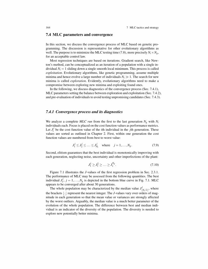
Figure 7.1 illustrates the J-values of the first regression problem in Sec. 2.3.1.The performance of MLC may be assessed from the following quantities. The bestindividual J j

1, j = 1, . . . ,Ng is depicted in the bottom blue curve in Fig. 7.1. MLCappears to be converged after about 30 generations.

The whole population may be characterized by the median value J jbNi/2c, where

the brackets b·c represent the nearest integer. The J-values vary over orders of mag-nitude in each generation so that the mean value or variances are strongly affectedby the worst outliers. Arguably, the median value is a much better parameter of theevolution of the whole population. The difference between best and median indi-vidual is an indicator of the diversity of the population. The diversity is needed toexplore new potentially better minima.

7.4 MLC parameters and convergence 165

— Minimal cost— Median cost— 1% limit— J(b = 0)

j

J

Fig. 7.1 MLC run for example in Sec. 2.3.1 featuring the best and median J-values In addition,the 1% limit indicates that all individuals above this line cumulate a 1% contribution to the geneticcontent of the next generation. The yellow line indicates the cost of all identically null individuals.

The diversity of the evolutionary process is also characterized by another J-value.The larger the J-value of an individual the less probable is the selection for anygenetic operation into the next generation. The J-value above which only 1% ofthe population is selected for an operation is called the 1% limit and displayed inFig. 7.1. This limit follows roughly the median in the presented example.

A peculiar feature of Fig. 7.1 is the yellow curve corresponding to the identicallyvanishing control function. This zero-individual can easily be produced from anyindividual by multiplying it with 0.

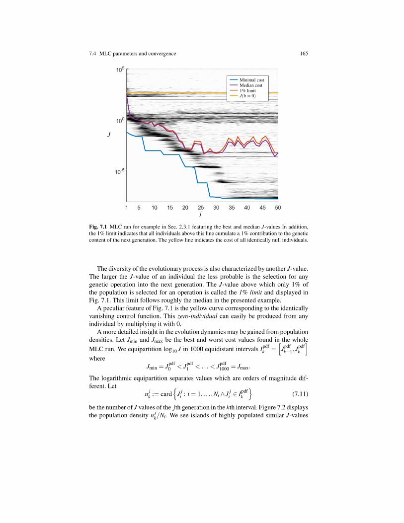
A more detailed insight in the evolution dynamics may be gained from populationdensities. Let Jmin and Jmax be the best and worst cost values found in the wholeMLC run. We equipartition log10 J in 1000 equidistant intervals Ipdf

k =h

Jpdfk�1,J

pdfk

i

whereJmin = Jpdf

0 < Jpdf1 < .. . < Jpdf

1000 = Jmax.

The logarithmic equipartition separates values which are orders of magnitude dif-ferent. Let

n jk := card

n

J ji : i = 1, . . . ,Ni ^ J j

i 2 Ipdfk

o

(7.11)

be the number of J values of the jth generation in the kth interval. Figure 7.2 displaysthe population density n j

k/Ni. We see islands of highly populated similar J-values


%of

pop.

j

J

(a)

Fig. 7.2 Same MLC run as in Fig. 7.1 but with a 3-dimensional view of the population den-sity (7.11).

over several generations. These islands tend to get initially increasingly populateduntil better islands are discovered.

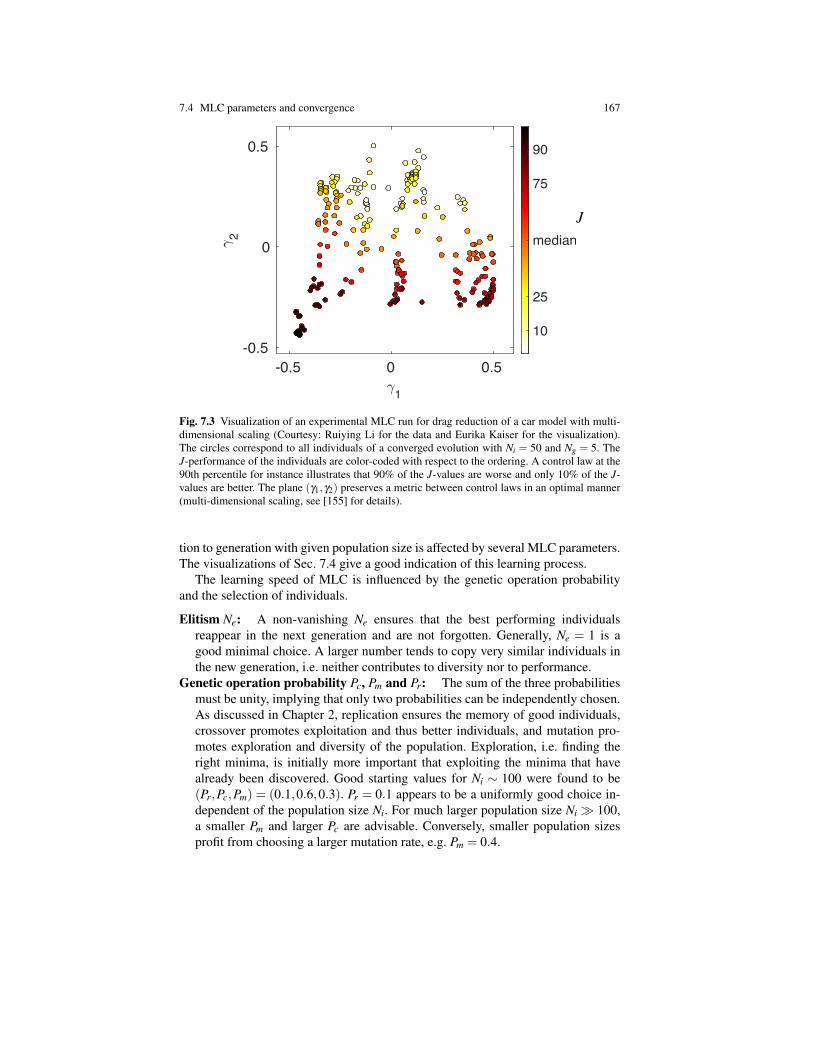
The evolution of the generations can be beautifully visualized with multi-dimen-sional scaling. This leads to a mathematically well-defined illustration of the princi-ple sketch of Fig. 2.12, i.e. indicates the landscape of J spanned by the population ofcontrol laws. Let Ki(s) denote the ith control law of an MLC run, i.e. i = 1, . . . ,Ni Ng.Let g i =

�

g i1,g i

2�

be a two-dimensional vector corresponding to the control law. LetDi j = hkKi(s)� K j(s)ki be a suitable metric between the ith and jth control law.Kaiser et al. suggest such a metric in [155]. Then multi-dimensional scaling pro-vides a configuration of g i which optimally preserves the metric kg i � g jk ⇡ Di j.Figure 7.3 shows an example of a closed-loop control experiment targeting dragreduction of a car model. The illustration indicates a clustering and scattering ofcontrol laws with an apparent minima in the lower left corner. Similar visualizationsof other MLC experiments showed far more complex topologies. The understandingof these topologies is still a subject of active research.

7.4.2 Parameters

As outlined in Sec. 7.3.3, a large population size Ni promotes exploration while along evolution Ng supports convergence. In addition, the learning rate from genera-

7.4 MLC parameters and convergence 167

.1

-0.5 0 0.5

.2

-0.5

0

0.5

10

25

median

75

90

J

Fig. 7.3 Visualization of an experimental MLC run for drag reduction of a car model with multi-dimensional scaling (Courtesy: Ruiying Li for the data and Eurika Kaiser for the visualization).The circles correspond to all individuals of a converged evolution with Ni = 50 and Ng = 5. TheJ-performance of the individuals are color-coded with respect to the ordering. A control law at the90th percentile for instance illustrates that 90% of the J-values are worse and only 10% of the J-values are better. The plane (g1,g2) preserves a metric between control laws in an optimal manner(multi-dimensional scaling, see [155] for details).

tion to generation with given population size is affected by several MLC parameters.The visualizations of Sec. 7.4 give a good indication of this learning process.

The learning speed of MLC is influenced by the genetic operation probabilityand the selection of individuals.

Elitism Ne: A non-vanishing Ne ensures that the best performing individualsreappear in the next generation and are not forgotten. Generally, Ne = 1 is agood minimal choice. A larger number tends to copy very similar individuals inthe new generation, i.e. neither contributes to diversity nor to performance.

Genetic operation probability Pc, Pm and Pr: The sum of the three probabilitiesmust be unity, implying that only two probabilities can be independently chosen.As discussed in Chapter 2, replication ensures the memory of good individuals,crossover promotes exploitation and thus better individuals, and mutation pro-motes exploration and diversity of the population. Exploration, i.e. finding theright minima, is initially more important that exploiting the minima that havealready been discovered. Good starting values for Ni ⇠ 100 were found to be(Pr,Pc,Pm) = (0.1,0.6,0.3). Pr = 0.1 appears to be a uniformly good choice in-dependent of the population size Ni. For much larger population size Ni � 100,a smaller Pm and larger Pc are advisable. Conversely, smaller population sizesprofit from choosing a larger mutation rate, e.g. Pm = 0.4.


Selection: The arguments of the genetic operations are determined by a stochasticselection process of the individuals. Like genetic operations, the selection maypromote exploitation or exploration. The harsher the bias towards best perform-ing individuals, the larger the probability that the local minima will be exploited.The individuals are chosen with equal probability in a tournament type selec-tion. The harshness of the selection is set by the tournament size. Setting Np = 7,enforces that the upper 50% of the current population accounts for the geneticcontent of 99% of the next generation for Ni = 100.

7.4.3 Pre-evaluation

The initial generation is composed of randomly chosen individuals. Evidently, onecan expect that most individuals are non-performing, probably performing worsethan the zero-individual b ⌘ 0. If random control laws would improve the cost func-tion, then control design would be simple.

Hence, a pre-evaluation of initial individuals is advised. Zero-individuals, for in-stance, should be replaced by other random individuals. Constant individuals mightalso be excluded, depending on the control problem. Non-trivial individuals maybe excluded if typical sensor readings lead to function values or function behaviorswhich are clearly out of bound in terms of amplitude or frequency content. The del-icate aspect is that the sensor readings change under actuation and a good guess ofthe probability distribution of sensor readings p(s) is required.

Another strategy to avoid the testing of non-promising individuals is to reducethe number of operations per individuals for instance by low initial tree depth forthe first generation.

Advanced material 7.1 Pre-evaluation in OpenMLC.

A more proactive measure can be undertaken by the use of a pre-evaluation function. Thisfunction takes the individual as an argument and returns a simple logical. If ‘false’ is re-turned, the individual is discarded and a new one is generated (or evolved). Detection ofzero-individuals can usually be easily achieved with a simple simplification of the LISPexpression (OpenMLC provides the function simplify_my_LISP.m). Saturated controllaws can be detected by providing random time series’ covering the whole sensor range forall sensors and discarding the control laws that stay constant (or keep the same value morethan a pre-determined percentage of the total samples).

7.5 The imperfect experiment 169

7.5 The imperfect experiment

Finally, we discuss the performance of MLC under imperfections of the experi-ments, like high-frequency noise (Sec. 7.5.1), low-frequency drift (Sec. 7.5.2), andthe need to monitor the experiment’s health status (Sec. 7.5.3).

7.5.1 Noise

In turbulence, noise is not an imperfection, but an intrinsic feature. For the purposeof control, we consider noise as the high-frequency fluctuations which are not rele-vant for the actuation mechanism. Noise impacts two aspects of MLC, the actuationcommand and the cost function. The actuation command b = K(s) is affected bynoise in the sensor signals. Every operation in the expression tree for K can act asnoise amplifier and at some complexity the control law may become a noise gen-erator. Hence, the number of operations or the depth of expression tree needs to belimited.

Second, the impact of noise on the cost function is far less critical, as the corre-sponding integrand is generally simple and the noise is largely integrated out.

The use of filters may improve MLC performance. Examples are low-pass, band-pass or single-frequency Morlet filters. We emphasize, again, that any predeter-mined filter introduces a bias towards the expected actuation mechanism which isnot necessarily the most effective one. The choice of the proper filter may also beintegrated in the MLC search algorithm like in Chapter 4.

7.5.2 Drift

Low-frequency drifts may arise due to changing operating conditions, e.g. changingoncoming velocity, temperature change or varying hot-wire anemometer readings.Drifts imply that effective individuals may degrade in performance and ineffectiveindividuals may improve. Drifts may also lead to the choice of different sensors inthe best control laws. However, within one or few generations, MLC will adjust tothe new operating conditions if the change in performance of a given individual isslow with respect to the testing time of one generation. If the change is significantlyfaster, the cost function values of a single generation are wrong and lead inevitablyto a poor ordering.

The cure for drifts depends on the cause. If the sensor readings drift, a re-calibration in regular intervals is advised. If the cost function drifts, the cure may bea normalization with the flow response to a periodic forcing. If the drifts are mea-sured, like the oncoming velocity, the parameter may be integrated into the controllaw. We shall not pause to give a more exhausting list of drifts and potential cures.


7.5.3 Monitoring

Finally, a MLC run may be a time-consuming experiment with complex instal-lations. Apart from slow drifts, there may be sudden unintended changes of theequipment. One or several hot-wire sensors may break. A pressure sensor may getclogged. An actuator may fail. Or there may be a sudden drop in the pressure reser-voir of the actuator leading to significantly reduced actuator efficiency. Parts ofequipment may unintentionally vibrate for some control laws. And the list can beindefinitely continued. Hence, an automatic extensive health monitoring of the plantis strongly advised to avoid extensive time on unsatisfying results. The authors haveexperienced several times that MLC has exploited weaknesses of problem defini-tion, the wind tunnel or the actuator setup. It is a common experience that controloptimization exploits the weakest links of the theoretical problem formulation / con-traints or imperfections of the plant.

chapter 7 mlc tactics and strategy - university of...

Documents