57

Chapter 6

Shear locking

In the preceding chapter, we saw a Ritz approximation of the Timoshenko beamproblem and noted that it was necessary to ensure a certain consistentrelationship between the trial functions to obtain accurate results. We shallnow take up the finite element representation of this problem, which isessentially a piecewise Ritz approximation. Our conclusions from the precedingchapter would therefore apply to this as well.

6.1 The linear Timoshenko beam element

An element based on elementary theory needs two nodes with 2 degrees of freedomat each node, the transverse deflection w and slope dw/dx and uses cubicinterpolation functions to meet the C1 continuity requirements of this theory(Fig. 6.1). A similar two-noded beam element based on the shear flexibleTimoshenko beam theory will need only C0 continuity and can be based on simplelinear interpolations. It was therefore very attractive for general purposeapplications. However, the element was beset with problems, as we shallpresently see.

6.1.1 The conventional formulation of the linear beam element

The strain energy of a Timoshenko beam element of length 2l can be written asthe sum of its bending and shear components as,

( )dxkGA21EI21 TT� + γγχχ (6.1)

where

x,θχ = (6.2a)

xw,−= θγ (6.2b)

In Equations (6.2a) and (6.2b), w is the transverse displacement and θ thesection rotation. E and G are the Young's and shear moduli and the shearcorrection factor used in Timoshenko's theory. I and A are the moment of inertiaand the area of cross-section, respectively.

(a) 1 2w ww,x w,x

(b) 1 2w wθ θ

Fig. 6.1 (a) Classical thin beam and (b) Timoshenko beam elements.

58

In the conventional procedure, linear interpolations are chosen for thedisplacement field variables as,

( ) 21N1 ξ−= (6.3a)

( ) 21N2 ξ+= (6.3b)

where the dimensionless coordinate ξ=x/l varies from -1 to +1 for an element oflength 2l. This ensures that the element is capable of strain free rigid bodymotion and can recover a constant state of strain (completeness requirement) andthat the displacements are continuous within the element and across the elementboundaries (continuity requirement). We can compute the bending and shearstrains directly from these interpolations using the strain gradient operatorsgiven in Equations (6.2a) and (6.2b). These are then introduced into the strainenergy computation in Equation (6.1), and the element stiffness matrix iscalculated in an analytically or numerically exact (a 2 point Gauss Legendreintegration rule) way.

For the beam element shown in Fig. 6.1, for a length h the stiffnessmatrix can be split into two parts, a bending related part and a shear relatedpart, as,

�������

�

�

�������

�

� −

=

������

�

�

������

�

�

−

−=

3h2h-6h2h

2h-12h-1-

6h2h-3h2h

2h12h1

hkGtk

1010

0000

1010

0000

hEIk

22

22

sb

We shall now model a cantilever beam under a tip load using this element,considering the case of a "thin" beam with E=1000, G=37500000, t=1, L=4, using afictitiously large value of G to simulate the "thin" beam condition. Table 6.1shows that the normalized tip displacements are dramatically in error. In factwith a classical beam element model, exact answers would have been obtained withone element for this case. We can carefully examine Table 6.1 to see the trendas the number of elements is increased. The tip deflections obtained, which areseveral orders of magnitude lower than the correct answer, are directly relatedto the square of the number of elements used for the idealization. In otherwords, the discretization process has introduced an error so large that the

resulting answer has a stiffness related to the inverse of N2. This is clearlyunrelated to the physics of the Timoshenko beam and also not the usual sort ofdiscretization errors encountered in the finite element method. It is this veryphenomenon that is known as shear locking.

Table 6.1 - Normalized tip deflections

No. of elements “Thin” beam1

2

4

816

0.200 × 10-5

0.800 × 10-5

0.320 × 10-4

0.128 × 10-3

0.512 × 10-3

59

The error in each element must be related to the element length, andtherefore when a beam of overall length L is divided into N elements of equallength h, the additional stiffening introduced in each element due to shearlocking is seen to be proportional to h2. In fact, numerical experiments showedthat the locking stiffness progresses without limit as the element depth tdecreases. Thus, we now have to look for a mechanism that can explain how this

spurious stiffness of (h/t)2 can be accounted for by considering the mathematicsof the discretization process.

The magic formula proposed to overcome this locking is the reducedintegration method. The bending component of the strain energy of a Timoshenkobeam element of length 2l shown in Equation (6.1) is integrated with a one-pointGaussian rule as this is the minimum order of integration required for exactevaluation of this strain energy. However, a mathematically exact evaluation ofthe shear strain energy will demand a two-point Gaussian integration rule. It isthis rule that resulted in the shear stiffness matrix of rank two that locked.An experiment with a one-point integration of the shear strain energy componentcauses the shear related stiffness matrix to change as shown below. Theperformance of this element was extremely good, showing no signs of locking atall (see Table 4.1 for a typical convergence trend with this element).

�������

�

�

�������

�

�

−

−−−

−

−

=

������

�

�

������

�

�

−

−=

4h2h4h2h

2h12h1

4h2h4h2h

2h12h1

hkGtk

1010

0000

1010

0000

hEIk

22

22

sb

6.1.2 The field-consistency paradigm

It is clear from the formulation of the linear Timoshenko beam element usingexact integration (we shall call it the field-inconsistent element) thatensuring the completeness and continuity conditions are not enough in someproblems. We shall propose a requirement for a consistent interpolation of theconstrained strain fields as the necessary paradigm to make our understanding ofthe phenomena complete.

If we start with linear trial functions for w and θ, as we had done inEquation 6.3 above, we can associate two generalized displacement constants witheach of the interpolations in the following manner

( )lxaaw 10 += (6.4a)

( )lxbb 10 +=θ (6.4b)

We can relate such constants to the field-variables obtaining in thiselement in a discretized sense; thus, a1/l=w,x at x=0, b0=θ and b1/l=θ,x at x=0.This denotation would become useful when we try to explain how thediscretization process can alter the infinitesimal description of the problem ifthe strain fields are not consistently defined.

60

If the strain-fields are now derived from the displacement fields given inEquation (6.4), we get

( )lb1=χ (6.5a)

( ) ( )lxblab 110 +−=γ (6.5b)

An exact evaluation of the strain energies for an element of length h=2l willnow yield the bending and shear strain energy as

( ) ( ) ( ){ } 21B lb2lEI21U = (6.6a)

( ) ( ) ( ){ }21

210s b31lab2lkGA21U +−= (6.6b)

It is possible to see from this that in the constraining physical limit of avery thin beam modeled by elements of length 2l and depth t, the shear strainenergy in Equation (6.6b) must vanish. An examination of the conditions producedby these requirements shows that the following constraints would emerge in sucha limit

0lab 10 →− (6.7a)

0b1 → (6.7b)

In the new terminology that we had cursorily introduced in Section 5.4,constraint (6.7a) is field-consistent as it contains constants from both thecontributing displacement interpolations relevant to the description of theshear strain field. These constraints can then accommodate the true Kirchhoffconstraints in a physically meaningful way, i.e. in an infinitesimal sense, thisis equal to the condition (θ-w,x)→0 at the element centroid. In direct

contrast, constraint (6.7b) contains only a term from the section rotation θ. Aconstraint imposed on this will lead to an undesired restriction on θ. In aninfinitesimal sense, this is equal to the condition θ,x→0 at the elementcentroid (i.e. no bending is allowed to develop in the element region). This isthe `spurious constraint' that leads to shear locking and violent disturbancesin the shear force prediction over the element, as we shall see presently.

6.1.3 An error model for the field-consistency paradigm

We must now determine that this field-consistency paradigm leads us to anaccurate error prediction. We know that the discretized finite element modelwill contain an error which can be recognized when digital computations madewith these elements are compared with analytical solutions where available. Theconsistency requirement has been offered as the missing paradigm for the error-free formulation of the constrained media problems. We must now devise anoperational procedure that will trace the errors due to an inconsistentrepresentation of the constrained strain field and obtain precise a priorimeasures for these. We must then show by actual numerical experiments with theoriginal elements that the errors are as projected by these a priori errormodels. Only such an exercise will complete the scientific validation of theconsistency paradigm. Fortunately, a procedure we shall call the functional re-constitution technique makes it possible to do this verification.

61

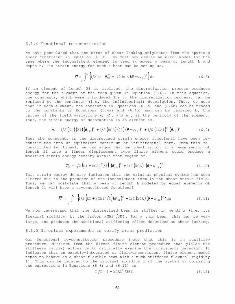
6.1.4 Functional re-constitution

We have postulated that the error of shear locking originates from the spuriousshear constraint in Equation (6.7b). We must now devise an error model for thecase where the inconsistent element is used to model a beam of length L anddepth t. The strain energy for such a beam can be set up as,

( ){ }� −+=L 2

x2x

0dxw,kGA21EI21 θθΠ , (6.8)

If an element of length 2l is isolated, the discretization process producesenergy for the element of the form given in Equation (6.6). In this equation,the constants, which were introduced due to the discretization process, can bereplaced by the continuum (i.e. the infinitesimal) description. Thus, we notethat in each element, the constants in Equations (6.6a) and (6.6b) can be tracedto the constants in Equations (6.4a) and (6.4b) and can be replaced by thevalues of the field variations θ, θ,x and w,x at the centroid of the element.Thus, the strain energy of deformation in an element is,

( ) ( ) ( ) ( ) ( ) ( ) ( ) ( )2x22

x2

xe ,kGAl61w,2lkGA21,2lEI21 θθθπ +−+= (6.9)

Thus the constants in the discretized strain energy functional have been re-constituted into an equivalent continuum or infinitesimal form. From this re-constituted functional, we can argue that an idealization of a beam region oflength 2l into a linear displacement type finite element would produce amodified strain energy density within that region of,

( ) ( ) ( ) ( )2x2

x2

e w,kGA21,3kGAlEI21 −++= θθπ (6.10)

This strain energy density indicates that the original physical system has beenaltered due to the presence of the inconsistent term in the shear strain field.Thus, we can postulate that a beam of length L modeled by equal elements oflength 2l will have a re-constituted functional

( ) ( ) ( ) ( ){ } dxw,kGA21,3kGAlEI21L 2

x2

x2

0� −++= θθΠ (6.11)

We now understand that the discretized beam is stiffer in bending (i.e. its

flexural rigidity) by the factor 3EIkGAl2 . For a thin beam, this can be very

large, and produces the additional stiffening effect described as shear locking.

6.1.5 Numerical experiments to verify error prediction

Our functional re-constitution procedure (note that this is an auxiliaryprocedure, distinct from the direct finite element procedure that yields thestiffness matrix) allows us to critically examine the consistency paradigm. Itindicates that an exactly-integrated or field-inconsistent finite element modeltends to behave as a shear flexible beam with a much stiffened flexural rigidityI’. This can be related to the original rigidity I of the system by comparingthe expressions in Equations (6.8) and (6.11) as,

3EIkGAL1II 2+=′ (6.12)

62

We must now show through a numerical experiment that this estimate for theerror, which has been established entirely a priori, starting from theconsistency paradigm and introducing the functional re-constitution technique,anticipates very accurately, the behavior of a field-inconsistent linearlyinterpolated shear flexible element in an actual digital computation. Exactsolutions are available for the static deflection W of a Timoshenko cantileverbeam of length L and depth t under a vertical tip load. If femW is the result

from a numerical experiment involving a finite element digital computation usingelements of length 2l, the additional stiffening can be described by a parameteras,

1WWe femfem −= (6.13)

From Equation (6.12), we already have an a priori prediction for this factor as,

3EIkGAl1IIe 2=−′= (6.14)

We can now re-interpret the results shown in Table 6.1 for the thin beamcase. Using Equations (6.13) and (6.14), we can argue a priori that theinconsistent element will produce normalized tip deflections ( ) ( )e11WWfem += .

Since e>>1, we have

( ) 52fem 105NWW −×= (6.15)

for the thin beam. Table 6.2 shows how the predictions made thus compare withthe results obtained from an actual finite element computation using the field-inconsistent element.

This has shown us that the consistency paradigm can be scientifically verified.Traditional procedures such as counting constraint indices, or computing therank or condition number of the stiffness matrices could offer only a heuristicpicture of how and why locking sets in.

It will be instructive to note here that conventional error analysis norms inthe finite element method are based on the percentage error or equivalent insome computed value as compared to the theoretically predicted value. We haveseen now that the error of shear locking can be exaggerated without limit, asthe structural parameter that acts as a penalty multiplier becomes indefinitely

Table 6.2 - Normalized tip deflections for the thin beam (Case 2) computed fromfem model and predicted from error model (Equation (6.15)).

N Computed (fem) Predicted

1

24

8

16

0.200 × 10-4

0.800 × 10-4

0.320 × 10-3

0.128 × 10-3

0.512 × 10-3

0.200 × 10-4

0.800 × 10-4

0.320 × 10-3

0.128 × 10-3

0.512 × 10-3

large. The percentage error norms therefore saturate quickly to a valueapproaching 100% and do not sensibly reflect the relationship between error andthe structural parameter even on a logarithmic plot. A new error norm called theadditional stiffening parameter, e can be introduced to recognize the manner inwhich the errors of locking kind can be blown out of proportion by a largevariation in the structural parameter. Essentially, this takes into account, thefact that the spurious constraints give rise to a spurious energy term andconsequently alters the rigidity of the system being modeled. In many otherexamples (e.g. Mindlin plates, curved beams etc.) it was seen that the rigidity,I, of the field consistent system and the rigidity, I’, of the inconsistent

system, were related to the structural parameters in the form, I’/I = α(l/t)2where l is an element dimension and t is the element thickness. Thus, if w isthe deflection of a reference point as predicted by an analytical solution tothe theoretical description of the problem and wfem is the fem deflectionpredicted by a field inconsistent finite element model, we would expect therelationship described by Equation 6.14. A logarithmic plot of the new errornorm against the parameter (l/t) will show a quadratic relationship that willcontinue indefinitely as (l/t) is increased. This was found to be true of themany constrained media problems. By way of illustration of the distinction made

Fig. 6.2 Variatcantil

63

ion of error norms e, E with structural parameter kGL2/Et2 for aever beam under tip shear force.

64

by this definition, we shall anticipate again, the results above. If werepresent the conventional error norm in the form ( ) WWWE fem−= , and plot both

E and the new error norm e from the results for the same problem using 4 FIelements against the penalty multiplier (l/t)2 on a logarithmic scale, thedependence is as shown in Fig. 6.2. It can be seen that E saturates quickly to avalue approaching 100% and cannot show meaningfully how the error propagates asthe penalty multiplier increases indefinitely. On the other hand, e capturesthis relationship, very accurately.

6.1.6 Shear Force Oscillations

A feature of inconsistently modeled constrained media problems is the presenceof spurious violently oscillating strains and stresses. It was not understoodfor a very long time that in many cases, stress oscillations originated from theinconsistent constraints. For a cantilever beam under constant bending momentmodeled using linear Timoshenko beam elements, the shear force (stresses)displays a saw-tooth pattern (we shall see later that a plane stress model using4-node elements will also give an identical pattern on the neutral bendingsurface). We can arrive at a prediction for these oscillations by applying thefunctional re-constitution technique.

If V is the shear force predicted by a field-consistent shear strainfield (we shall see soon how the field-consistent element can be designed) and Vthe shear force obtained from the original shear strain field, we can write fromEquation (6.5b),

( )labkGAV 10 −= (6.16a)

( )lxbkGAVV 1+= (6.16b)

We see that V has a linear term that relates directly to the constant thatappeared in the spurious constraint, Equation (6.7b). We shall see below fromEquation (6.17) that b1 will not be zero, in fact it is a measure of the bendingmoment at the centroid of the element. Thus, in a field-inconsistentformulation, this constant will activate a violent linear shear force variationwhen the shear forces are evaluated directly from the shear strain field givenin Equation (6.5b). The oscillation is self-equilibrating and does notcontribute to the force equilibrium over the element. However, it contributes afinite energy in Equation (6.9) and in the modeling of very slender beams, thisspurious energy is so large as to completely dominate the behavior of the beamand cause a locking effect.

Figure 6.3 shows the shear force oscillations in a typical problem - astraight cantilever beam with a concentrated moment at the tip. One to ten equallength field-inconsistent elements were used and shear forces were computed atthe nodes of each element. In each case, only the variation within the elementat the fixed end is shown, as the pattern repeats itself in a saw-tooth mannerover all other elements. At element mid-nodes, the correct shear force i.e. V=0is reproduced. Over the length of the element, the oscillations are seen to belinear functions corresponding to the kGA b1 (x/l) term. Also indicated by thesolid lines, is the prediction made by the functional re-constitution exercise.We shall explore this now.

Fig. 6.3 Shear forcemodels of a

Consider a straend. This should proshear force Q in thewill now respond in tthe average of the lelement. If the elem

after accounting forat the element centro

In a field-incoconsider the modified

to 1b ′ , that is,

where 3EIkGAle 2= .

Thus, in a fie

by the factor e; the

65

oscillations in element nearest the root, for N elementcantilever of length L = 60.

ight cantilever beam with a tip shear force Q at the freeduce a linearly varying bending moment M and a constantbeam. An element of length 2l at any station on the beamhe following manner. Since, a linear element is used, onlyinearly varying bending moment is expected in each finiteent is field-consistent, the constant b1 can be associated

discretization, to relate to the constant bending moment M0id as,

lbEIM 10 = or

EIlMb 01 = (6.17)

nsistent problem, due to shear locking, it is necessary toflexural rigidity I’ (see Equation 6.17) that modifies b1

IElMb 01 ′=′( ){ }e1EIlM0 +=

( )e1b1 += (6.18)

ld-inconsistent formulation, the constant b1 gets stiffened

constant bending moment M0 is also underestimated by the

66

same factor. Also, for a very thin beam where e>>1, the centroidal moment M0predicted by a field-consistent element diminishes in a t2 rate for a beam ofrectangular cross-section. These observations have been confirmed throughdigital computation.

The field-consistent element will respond with QVV 0 == over the entire

element length 2l. The field-inconsistent shear force V from Equations (6.16)and (6.18) can be written for a very thin beam (e>>1) as,

( ) ( )lxl3MQV 0+= (6.19)

These are the violent shear force linear oscillations within each element, whichoriginate directly from the field-inconsistency in the shear strain definition.

These oscillations are also seen if field-consistency had been achieved inthe element by using reduced integration for the shear strain energy. Unless theshear force is sampled at the element centroid (i.e. Gaussian point, x/l=0),these disturbances will be much more violent than in the exactly integratedversion.

6.1.7 The consistent formulation of the linear element

We can see that reduced integration ensures that the inconsistent constraintdoes not appear and so is effective in producing a consistent element, at leastin this instance. We must now satisfy ourselves that such a modification did notviolate any variational theorem.

The field-consistent element, as we now shall call an element version freeof spurious (i.e. inconsistent) constraints, can and has been formulated invarious other ways as well. The `trick' is to evaluate the shear strain energy,in this instance, in such a way that only the consistent term will contribute tothe shear strain energy. Techniques like addition of bubble modes, hybridmethods etc. can produce the same results, but in all cases, the need forconsistency of the constrained strain field must be absolutely met.

We explain now why the use of a trick like the reduced integrationtechnique, or the use of assumed strain methods allows the locking problem to beovercome. It is obvious that it is not possible to reconcile this within theambit of the minimum total potential principle only, which had been the startingpoint of the conventional formulation.

We saw in Chapter 2, an excellent example of a situation where it wasnecessary to proceed to a more general theorem (one of the so-called mixedtheorems) to explain why the finite element method computed strain and stressfields in a `best-fit' sense. We can now see that in the case of constrainedmedia problems, the mixed theorem such as the Hu-Washizu or Hellinger-Reissnertheorem can play a crucial role in proving that by modifying the minimum totalpotential based finite element formulation by using an assumed strain field toreplace the kinematically derived constrained field, no energy, or workprinciple or variational norms have been violated.

67

To eliminate problems such as locking, we look for a consistentconstrained strain field to replace the inconsistent kinematically derivedstrain field in the minimum total potential principle. By closely examining thestrain gradient operators, it is possible to identify the order up to which theconsistent strain field must be interpolated. In this case, for the lineardisplacement interpolations, Equations (6.5b), (6.7a) and (6.7b) tell us thatthe consistent interpolation should be a constant. At this point we shall stillnot presume what this constant should be, although past experience suggests itis the same constant term seen in Equation (6.7a). Instead, we bring in theHellinger-Reissner theorem in the following form to see the identity of theconsistent strain field clearly. For now, it is sufficient to note that theHellinger-Reissner theorem is a restricted case of the Hu-Washizu theorem. Inthis theorem, the functional is stated in the following form,

( )dxkGAkGA21EIEI21 TTTT� +−+− γγγγχχχχ (6.20)

where χ and γ are the new strain variables introduced into this multi-field

principle. Since we have difficulty only with the kinematically derived γ we canhave χχ = and recommend the use of a γ which is of consistent order to replace

γ. A variation of the functional in Equation (6.20) with respect to the as yetundetermined coefficients in the interpolation for γ yields

( )� =− 0dxT γγγδ (6.21)

This orthogonality condition now offers a means to constitute the coefficientsof the consistent strain field from the already known coefficients of thekinematically derived strain field. Thus, for γ given by Equation (6.5b), it ispossible to show that ( )lb 10 αγ −= . In this simple instance, the same result is

obtained by sampling the shear strain at the centroid, or by the use of one-point Gaussian integration. What is important is that, deriving the consistentstrain-field using this orthogonality relation and then using this to computethe corresponding strain energy will yield a field-consistent element which doesnot violate any of the variational norms, i.e. an exact equivalence to the mixedelement exists without having to go through the additional operations in a mixedor hybrid finite element formulation, at least in this simple instance. We saythat the variational correctness of the procedure is assured. The substitutestrain interpolations derived thus can therefore be easily coded in the form ofstrain function subroutines and used directly in the displacement type elementstiffness derivations.

6.1.8 Some concluding remarks on the linear beam element

So far we have seen the linear beam element as an example to demonstrate theprinciples involved in the finite element modeling of a constrained mediaproblem. We have been able to demonstrate that a conceptual framework thatincludes a condition that specifies that the strain fields which are to beconstrained must satisfy a consistency criterion is able to provide a completescientific basis for the locking problems encountered in conventionaldisplacement type modeling. We have also shown that a correctness criterion(which links the assumed strain variation of the displacement type formulation

68

to the mixed variational theorems) allows us to determine the consistent strainfield interpolation in a unique and mathematically satisfying manner.

It will be useful now to see how these concepts work if a quadratic beamelement is to be designed. This is a valuable exercise as later, the quadraticbeam element shall be used to examine problems such as encountered in curvedbeam and shell elements and in quadrilateral plate elements due to non-uniformmapping.

6.2 The quadratic Timoshenko beam element

We shall now very quickly see how the field-consistency rules explain thebehavior of a higher order element. We saw in Chapter 5 that the conventionalformulation with lowest order interpolation functions led to spuriousconstraints and a non-singular assembled stiffness matrix, which result inlocking. In a higher order formulation, the matrix was singular but the spuriousconstraints resulted in a system that had a higher rank than was felt to bedesirable. This resulted in sub-optimal performance of the approximation. We cannow use the quadratic beam element to demonstrate that this is true in finiteelement approximations as well.

6.2.1 The conventional formulation

Consider a quadratic beam element designed according to conventional principles,i.e. exact integration of all energy terms arising from a minimum totalpotential principle. As the beam becomes very thin, the element does not lock;in fact it produces reasonably meaningful results. Fig. 6.4 shows a typicalcomparison between the linear and quadratic beam elements in its application toa simple problem. A uniform cantilever beam of length 1.0 m, width 0.01 m anddepth 0.01 m has a vertical tip load of 100 N applied at the tip. For E=1010

N/m2 and µ=0.3, the engineering theory of beams predicts a tip deflection ofw=4.0 m. We shall consider three finite element idealizations of this problem -with the linear 2-node field-consistent element considered earlier in thissection (2C, on the Figure), the quadratic 3-node field-inconsistent elementbeing discussed now (3I, on the Figure) and the quadratic 3-node field-consistent element which we shall derive later (3C). It is seen that for thissimple problem, the 3C element produces exact results, as it is able to simulatethe constant shear and linear bending moment variation along the beam length.The 3I and 2C elements show identical convergence trends and behave as if theyare exactly alike. The curious aspects that call for further investigation are:the quadratic element (3I) behaves in exactly the same way as the field-consistent linear element (2C), giving exactly the same accuracy for the samenumber of elements although the system assembled from the former had nearlytwice as many nodes. It also produced moment predictions, which were identical,i.e., the quadratic beam element, instead of being able to produce linear-accurate bending moments could now yield only a constant bending moment withineach element, as in the field-consistent linear element. Further, there were nowquadratic oscillations in the shear force predictions for such an element. Notenow that these curious features cannot be explained from the old arguments,which linked locking to the non-singularity or the large rank or the spectralcondition number of the stiffness matrix. We shall now proceed to explain thesefeatures using the field-consistency paradigm.

Fig.conve

If quadraticand θ in the followi

the shear strain int

γ

Again, we emphasizeLegendre polynomialorthogonal nature obecomes the sum ofpolynomials. Indeed,

21Us =

Therefore, whbeam the shear straof the strain fieldseparately. In this

69

6.4 A uniform cantilever beam with tip shear force -rgence trends of linear and quadratic elements.

isoparametric functions are used for the field-variables wng manner

( ) ( )2210 lxalxaaw ++=

( ) ( )2210 lxblxbb ++=θ

erpolation will be,

( ) ( ) ( )2221120 313bl2abla3bb ξξ −−−+−+= (6.22)

the usefulness of expanding the strain field in terms of thes. When the strain energies are integrated, because of thef the Legendre polynomials the discretized energy expressionthe squares of the coefficients multiplying the Legendrethe strain energy due to transverse shear strain is,

( ) ( ) ( ) ( ){ }454bl2ab31la3bb2lkGA 22

221

2120 +−+−+ (6.23)

en we introduce the penalty limit condition that for a thinin energies must vanish, we can argue that the coefficientsexpanded in terms of the Legendre polynomials must vanishcase, three constraints emerge:

( ) 0la3bb 120 →−+ (6.24a)

70

( ) 0l2ab 21 →− (6.24b)

0b2 → (6.24c)

Equations (6.24a) and (6.24b) represent constraints having contributionsfrom the field interpolations for both w and θ. They can therefore reproduce, ina consistent manner, true constraints that reflect a physically meaningfulimposition of the thin beam Kirchhoff constraint. This is therefore the field-consistent part of the shear strain interpolation.

Equation (6.24c) however contains a constant only from the interpolationfor θ. This constraint, when enforced, is an unnecessary restriction on thefreedom of the interpolation for θ, constraining it in fact to behave only as a

linear interpolation as the constraint implies that θ,xx→0 in a discretizedsense over each beam element region. The spurious energy implied by such aconstraint does not contribute directly to the discretized bending energy,unlike the linear beam element seen earlier. Therefore, field-inconsistency inthis element would not cause the element to lock. However, it will diminish therate of convergence of the element and would induce disturbances in the form ofviolent quadratic oscillations in the shear force predictions, as we shall seein the next section.

6.2.2 Functional reconstitution

We can use the functional re-constitution technique to see how theinconsistent terms in the shear strain interpolation alter the description ofthe physics of the original problem (we shall skip most of the details, as thematerial is available in greater detail in Ref. 6.1).

The b2 term that appears in the bending energy also makes an appearance inthe shear strain energy, reflecting its origin through the spurious constraint.We can argue that this accounts for the poor behavior of the field-inconsistentquadratic beam element (the 3I of Fig. 6.4). Ref. 6.1 derives the effect moreprecisely, demonstrating that the following features can be fully accounted for:

i) the displacement predictions of the 3I element are identical to that made bythe 2C element on an element by element basis although it has an additional mid-node and has been provided with the more accurate quadratic interpolationfunctions.ii) the 3I element can predict only a constant moment within each element,exactly as the 2C element does.iii) there are quadratic oscillations in the shear force field within eachelement.

We have already discussed earlier that the 3I element (the field-inconsistent 3-noded quadratic) converges in exactly the same manner as the 2Celement (the field-consistent linear). This has been explained by showing using

the functional re-constitution technique, that the b2 term, which describes thelinear variation in the bending strain and bending moment interpolation, is"locked" to a vanishingly small value. The 3I element then effectively behavesas a 2C element in being able to simulate only a constant bending-moment in eachregion of a beam, which it replaces.

71

6.2.3 The consistent formulation of the quadratic element

As in the linear element earlier, the field-consistent element (3C) can beformulated in various ways. Reduced integration of the shear strain energy usinga 2-point Gauss-Legendre formula was the most popular method of deriving theelement so far. Let us now derive this element using the `assumed' strainapproach. We use the inverted commas to denote that the strain is not assumed inan arbitrary fashion but is actually uniquely determined by the consistency andthe variational correctness requirements. The re-constitution of the field is tobe done in a variationally correct way, i.e. we are required to replace γ inEquation (6.22) which had been derived from the kinematically admissibledisplacement field interpolations using the strain-displacement operators withan `assumed' strain field γ which contains terms only upto and including the

linear Legendre polynomial in keeping with the consistency requirement. Let uswrite this in the form

ξγ 10 cc += (6.25)

The orthogonality condition in Equation (6.21) dictates how γ should replace γover the length of the element. This determines how c0 and c1 should be

constituted from b0, b1 and b2. Fortunately, the orthogonal nature of theLegendre polynomials allows this to be done for this example in a very trivialfashion. The quadratic Legendre polynomial and its coefficient are simply

truncated and c0=b0 and c1=b1 represent the variationally correct field-consistent `assumed' strain field. The use of such an interpolation subsequentlyin the integration of the shear strain energy is identical to the use of reducedintegration or the use of a hybrid assumed strain approach. In a hybrid assumedstrain approach, such a consistent re-constitution is automatically implied inthe choice of assumed strain functions and the operations leading to thederivation of the flexibility matrix and its inversion leading to the finalstiffness matrix.

6.3 The Mindlin plate elements

A very large part of structural analysis deals with the estimation of stressesand displacements in thin flexible structures under lateral loads using what iscalled plate theory. Thus, plate elements are the most commonly used elements ingeneral purpose structural analysis. At first, most General Purpose Packages(GPPs) for structural analysis used plate elements based on what are called theC1 theories. Such theories had difficulties and limitations and a1so attention

turned to what are called the C0 theories.

The Mindlin plate theory [6.2] is now the most commonly used basis for thedevelopment of plate elements, especially as they can cover applications tomoderately thick and laminated plate and shell constructions. It has beenestimated that in large scale production runs using finite element packages, thesimple four-node quadrilateral plate element (the QUAD4 element) may account foras much as 80% of all usage. It is therefore important to understand that theevolution of the current generation of QUAD4 elements from those of yester-year,over a span of nearly three decades was made difficult by the presence of shearlocking. We shall now see how this takes place.

72

The history behind the discovery of shear locking in plate elements isquite interesting. It was first recognized when an attempt was made to representthe behavior of shells using what is called the degenerate shell approach [6.3].In this the shell behavior is modeled directly after a slight modification ofthe 3D equations and shell geometry and domain are represented by a 3D brickelement but its degrees of freedom are condensed to three displacements and twosection rotations at each node. Unlike classical plate or shell theory, thetransverse shear strain and its energy is therefore accounted for in thisformulation. Such an approach was therefore equivalent to a Mindlin theoryformulation. These elements behaved very poorly in representing even the trivialexample of a plate in bending and the errors progressed without limit, as theplates became thinner. The difficulty was attributed to shear locking. This isin fact the two-dimensional manifestation of the same problem that weencountered for the Timoshenko beam element; ironically it was noticed first inthe degenerate shell element and was only later related to the problems indesigning Timoshenko beam and Mindlin plate elements [6.4]. The remedy proposedat once was the reduced integration of the shear strain energy [6.5,6.6]. Thiswas only partially successful and many issues remained unresolved. Some of thesewere,

i) the 2×2 rule failed to remove shear locking in the 8-node serendipity plateelement,ii) the 2×2 rule in the 9-node Lagrangian element removed locking but introducedzero energy modes,iii) the selective 2×3 and 3×2 rule for the transverse shear strain energies

from γxz and γyz recommended for a 8-node element also failed to remove shearlocking,iv) the same selective 2×3 and 3×2 rule when applied to a 9-noded element isoptimal for a rectangular form of the element but not when the element wasdistorted into a general quadrilateral form,v) even after reduced integration of the shear energy terms, the degenerateshell elements performed poorly when trying to represent the bending of curvedshells, due to an additional factor, identified as membrane locking [6.7],originating now from the need for consistency of the membrane straininterpolations. We shall consider the membrane-locking phenomenon in anothersection.

We shall confine our study now to plate elements without going into thecomplexities of the curved shell elements.

In Kirchhoff-Love thin plate theory, the deformation is completelydescribed by the transverse displacement w of the mid-surface. In such adescription, the transverse shear deformation is ignored. To account fortransverse shear effects, it is necessary to introduce additional degrees offreedom. We shall now consider Mindlin's approximations, which have permittedsuch an improved description of plate behavior. The degenerate shell elementsthat we discussed briefly at the beginning of this section can be considered tocorrespond to a Mindlin type representation of the transverse shear effects.

In Mindlin's theory [6.2], deformation is described by three quantities,the section rotations θx and θy (i.e. rotations of lines normal to themidsurface of the undeformed plate) and the mid-surface deflection w. Thebending strains are now derived from the section rotations and do not cause any

73

difficulty when a finite element model is made. The shear strains are nowcomputed as the difference between the section rotations and the slopes of theneutral surfaces, thus,

xxxz w,−= θγ

yyyz w,−= θγ (6.26)

The stiffness matrix of a Mindlin plate element will now have terms from thebending strain energy and the shear strain energy. It is the inconsistentrepresentation of the latter that causes shear locking.

6.3.1 The 4-node plate element

The 4-node bi-linear element is the simplest element based on Mindlin theorythat could be devised. We shall first investigate the rectangular form of theelement [6.4] as it is in this configuration that the consistency requirementscan be easily understood and enforced. In fact, an optimum integration rule canbe found which ensures consistency if the element is rectangular. It wasestablished in Ref. 6.4 that an exactly integrated Mindlin plate element wouldlock even in its rectangular form. Locking was seen to vanish for therectangular element if the bending energy was computed with a 2×2 Gaussianintegration rule while a reduced 1-point rule was used for the shear strainenergy. This rectangular element behaved very well if the plate was thin but theresults deteriorated as the plate became thicker. Also, after distortion to aquadrilateral form, locking re-appeared. A spectral analysis of the elementstiffness matrix revealed a rank deficiency - there were two zero energymechanisms in addition to the usual three rigid body modes required for such anelement. It was the formation of these mechanisms that led to the deteriorationof element performance if the plate was too thick or if it was very looselyconstrained. It was not clear why the quadrilateral form locked even afterreduced integration. We can now demonstrate from our consistency view-point whythe 1-point integration of the shear strain energy is inadequate to retain allthe true Kirchhoff constraints in a rectangular thin plate element. However, weshall postpone the discussion on why such a strategy cannot preserve consistencyif the element was distorted to a later section.

Following Ref. [6.4], the strain energy for an isotropic, linear elasticplate element according to Mindlin theory can be constituted from its bendingand shear energies as,

SB UUU +=

( ) [{� � ++−

= yyxxy2yx

2x2

2

2,,124

Et ,, θθνθθν

( ) ( ) ] dydx21 2xy,yx, θθν +−+ (6.27)

( ) ( ) ( )[ ] }� � −+−−+ dydxw,w,t

16k 2yy

2xx2

θθν

74

Fig. 6.5 Cartesian and natural coordinate system for a four-node rectangularplate element.

where x, y are Cartesian co-ordinates (see Fig. 6.5), w is the transversedisplacement, θx and θy are the section rotations, E is the Young's modulus, νis the Poisson's ratio, k is the shear correction factor and t is the platethickness. The factor k is introduced to compensate for the error inapproximating the shear strain as a constant over the thickness direction of aMindlin plate.

Let us now examine the field-consistency requirements for one of the shearstrains, γxz, in the Cartesian system. The admissible displacement fieldinterpolations required for a 4-node element can be written in terms of theCartesian co-ordinates itself as,

xyayaxaaw 3210 +++= (6.28a)

xybybxbb 3210 +++=θ (6.28b)

The shear strain field derived from these kinematically admissible shapefunctions is,

( ) ( ) xybxbyabab 313210xz ++−+−=γ (6.29)

As the plate thickness is reduced to zero, the shear strains must vanish. Thediscretized constraints that are seen, to be enforced as 0xz →γ in Equation

(6.29) are,0ab 10 →− (6.30a)

0ab 32 →− (6.30b)

0b1 → (6.30c)

0b3 → (6.30d)

75

The constraints shown in Equations (6.30a) and (6.30b) are physically meaningfuland represent the Kirchhoff condition in a discretized form. Constraints (6.30c)and (6.30d) are the cause for concern here - these are the spurious or`inconsistent' constraints which lead to shear locking. Thus, in a rectangularelement, the requirement for consistency of the interpolations for the shearstrains in the Cartesian co-ordinate system is easily recognized as thepolynomials use only Cartesian co-ordinates. Let us now try to derive theoptimal element and also understand why the simple 1-point strategy of Ref. 6.4led to zero energy mechanisms.

It is clear from Equations (6.29) and (6.30) that the terms b1x and b3xyare the inconsistent terms which will contribute to locking in the form ofspurious constraints. Let us now look for optimal integration strategies forremoving shear locking without introducing any zero energy mechanisms. We shallconsider first, the part of the shear strain energy contributed by γxz. We must

integrate exactly, terms such as (b0-a1), (b2-a3)y, b1x, and b3xy. We now

identify terms such as (b0-a1), (b2-a3), b1, and b3 as being equivalent to the

quantities (θx-w,x)0, (θx-w,x),y0, (θx,x)0, and (θx,xy)0 where the subscript ‘0’denotes the values at the centroid of the element (for simplicity, we let thecentroid of the element lie at the origin of the Cartesian co-ordinate system).

An exact integration, that is a 2×2 Gaussian integration of the shearstrain energy leads to

( ) ( ) ( ) ( )[ ]� � ++−+−= 20xyx

2220xx

2y0

2xx

220xx

2xz ,9lh,3lw,3hw,4lhdydx θθθθγ , (6.31)

In the penalty limit of a thin plate, these four quantities act as constraints.The first two reproduce the true Kirchhoff constraints and the remaining two actas spurious constraints that cause shear locking by enforcing θx,x→0 and θx,xy→0in the element.

If a 1×2 Gaussian integration is used, we have,

( ) ( )[ ]� � −+−= y02

xx22

0xx2xz w,3hw,4lhdydx ,θθγ (6.32)

Thus, only the true constraints are retained and all spurious constraints areremoved. This strategy can also be seen to be variationally correct in thiscase; we shall see later that in a quadrilateral case, it is not possible toensure variational correctness exactly. By a very similar argument, we can showthat the part of the shear strain energy from γyz will require a 2×1 Gaussianintegration rule. This element would be the optimal rectangular bi-linearMindlin plate element.

Let us now look at the 1-point integration strategy used in Ref. 6.4. Thiswill give shear energy terms such as,

( )[ ]� � −= 20xx

2xz w,4lhdydx θγ (6.33)

76

We have now only one true constraint each for the shear energy from γxzand γyz respectively while the other Kirchhoff constraints ( ) 0w, y0xx →− ,θ and

( ) 0w, x0yy →− ,θ are lost. This introduces two zero energy modes and accounts for

the consequent deterioration in performance of the element when the plates arethick or are very loosely constrained, as shown in Ref. 6.4.

We have seen now that it is a very simple procedure to re-constitutefield-consistent assumed strain fields from the kinematically derived fieldssuch as shown in Equation (6.29) so that they are also variationally correct.This is not so simple in a general quadrilateral where the complication arisingfrom the isoparametric mapping from a natural co-ordinate system to a Cartesiansystem makes it very difficult to see the consistent form clearly. We shall seethe difficulties associated with this form in a later section.

6.3.2 The quadratic 8-node and 9-node plate elements

The 4-node plate element described above is based on bi-linear functions. Itwould seem that an higher order element based on quadratic functions would befar more accurate. There are now two possibilities, an 8-node element based onwhat are called the serendipity functions and a 9-node element based on theLagrangian bi-quadratic functions. There has been a protracted debate on whichversion is more useful, both versions having fiercely committed protagonists.By now, it is well known that the 9-node element in its rectangular form is freeof shear locking even with exact integration of shear energy terms and that itsperformance is vastly improved when its shear strain energies are integrated ina selective sense (2×3 and 3×2 rules for xzγ and yzγ terms respectively). It is

in fact analogous to the quadratic Timoshenko beam element, the field-inconsistencies not being severe enough to cause locking. This is however nottrue for the 8-node element which was derived from the Ahmad shell element [6.3]and which actually pre-dates the 4-node Mindlin element. An exact integration ofbending and shear strain energies resulted in an element that locked for mostpractical boundary suppressions even in its rectangular form. Many ad-hoctechniques e.g. the reduced and selective integration techniques, hybrid andmixed methods, etc. failed or succeeded only partially. It was thereforeregarded for some time as an unreliable element as no quadrature rule seemed tobe able to eliminate locking entirely without introducing other deficiencies. Itseems possible to attribute this noticeable difference in the performance of the8- and 9-node elements to the missing central node in the former. This makes itmore difficult to restore consistency in a simple manner.

6.3.3 Stress recovery from Mindlin plate elements

The most important information a structural analyst looks for in a typicalfinite element static analysis is the state of stress in the structure. It istherefore very important for one to know points of optimal stresses in theMindlin plate elements. It is known that the stress recovery at nodes fromdisplacement elements is unreliable, as the nodes are usually the points wherethe strains and stresses are least accurate. It is possible however to determinepoints of optimal stress recovery using an interpretation of the displacementmethod as a procedure that obtains strains over the finite element domain in aleast-squares accurate sense. In Chapter 2, we saw a basis for thisinterpretation. We can apply this rule to determine points of accurate stress

77

recovery in the Mindlin plate elements. For a field-consistent rectangular 4-node element, the points are very easy to determine [6.8] (note that in a field-inconsistent 4-node element, there will be violent linear oscillations in theshear stress resultants corresponding to the inconsistent terms). Thus, Ref. 6.8shows that bending moments and shear stress resultants Qxz and Qyz are accurate

at the centroid and at the 1×2 and 2×1 Gauss points in a rectangular element forisotropic or orthotropic material. It is coincidental, and therefore fortuitous,that the shear stress resultants are most accurate at the same points at whichthey must be sampled in a selective integration strategy to remove the field-inconsistencies! For anisotropic cases, it is safest to sample all stressresultants (bending and shear) at the centroid.

Such rules can be extended directly to the 9-node rectangular element. Thebending moments are now accurate at the 2×2 Gauss points and the shear stressresultants in an isotropic or orthotropic problem are optimal at the same 2×3and 3×2 Gauss points which were used to remove the inconsistencies from thestrain definitions. However, accurate recovery of stresses from the 8-nodeelement is still a very challenging task because of the difficulty informulating a robust element. The most efficient elements known today arevariationally incorrect even after being made field-consistent and need specialfiltering techniques before the shear stress resultants can be reliably sampled.

So far, discussion on stress sampling has been confined to rectangularelements. When the elements are distorted, it is no simple matter to determinethe optimal points for stress recovery - the stress analyst must then exercisecare in applying these rules to seek reliable points for recovering stresses.

6.4 Concluding remarks

We can conclude this section on shear locking by noting that the availableunderstanding was unable to resolve the phenomena convincingly. The proposedimprovement, which was the consistency paradigm, together with the functionalre-constitution procedure, allowed us to derive an error estimate for a caseunder locking and we could show through numerical (digital) experiments thatthese estimates were accurate. In this way we are convinced that a theory withthe consistency paradigm is more successful from the falsifiability point ofview than one without.

6.5 References

6.1 G. Prathap and C. R. Babu, Field-consistent strain interpolations for thequadratic shear flexible beam element, Int. J. Num. Meth. Engng. 23, 1973-1984, 1986.

6.2 R. D. Mindlin, Influence of rotary inertia and shear on flexural motion ofelastic plates, J. Appl. Mech. 18, 31-38, 1951.

6.3 S. Ahmad, B. M. Irons and O. C. Zienkiewicz, Analysis of thick and thinshell structures by curved finite elements, Int. J. Num. Meth. Engng. 2,419-451, 1970.

6.4 T. J. R. Hughes, R. L. Taylor and W. Kanoknukulchal, A simple and efficientfinite element for plate bending, Int. J. Num. Meth. Engng. 411, 1529-1543, 1977.

6.5 S. F. Pawsey and R. W. Clough, Improved numerical integration of thick shellfinite elements, Int. J. Num. Meth. Engng. 43, 575-586, 1971.

78

6.6 O. C. Zienkiewicz, R. L. Taylor and J. M. Too, Reduced integration techniquein general analysis of plates and shells, Int. J. Num. Meth. Engng. 43, 275-290, 1971.

6.7 H. Stolarski and T. Belytschko, Membrane locking and reduced ingression forcurved elements, J. Appl. Mech. 49, 172-178, 1982.

6.8 G. Prathap and C. R. Babu, Accurate force evaluation with a simple bi-linearplate bending element, Comp. Struct. 25, 259-270, 1987.