chapter 5 hashing - william & mary
TRANSCRIPT

Chapter 5
Hashing

Introduction
2
−hashing performs basic operations, such as insertion,
deletion, and finds in constant average time
−better than other ADTs we’ve seen so far

Hashing
3
−a hash table is merely an array of some fixed size
−hashing converts search keys into locations in a hash table
−searching on the key becomes something like array
lookup
−hashing is typically a many-to-one map: multiple keys are
mapped to the same array index
−mapping multiple keys to the same position results in a
collision that must be resolved
− two parts to hashing:
−a hash function, which transforms keys into array indices
−a collision resolution procedure

Hashing Functions
4
− let 𝐾 be the set of search keys
−hash functions map 𝐾 into the set of 𝑀 slots in the hash table
ℎ: 𝐾 → {0, 1, … ,𝑀 − 1}
− ideally, ℎ distributes 𝐾 uniformly over the slots of the hash table, to minimize collisions
− if we are hashing 𝑁 items, we want the number of items hashed to each location to be close to 𝑁/𝑀
−example: Library of Congress Classification System
−hash function if we look at the first part of the call numbers (e.g., E470, PN1995)
−collision resolution involves going to the stacks and looking through the books
−almost all of CS is hashed to QA75 and QA76 (BAD)
Hashing Functions
5
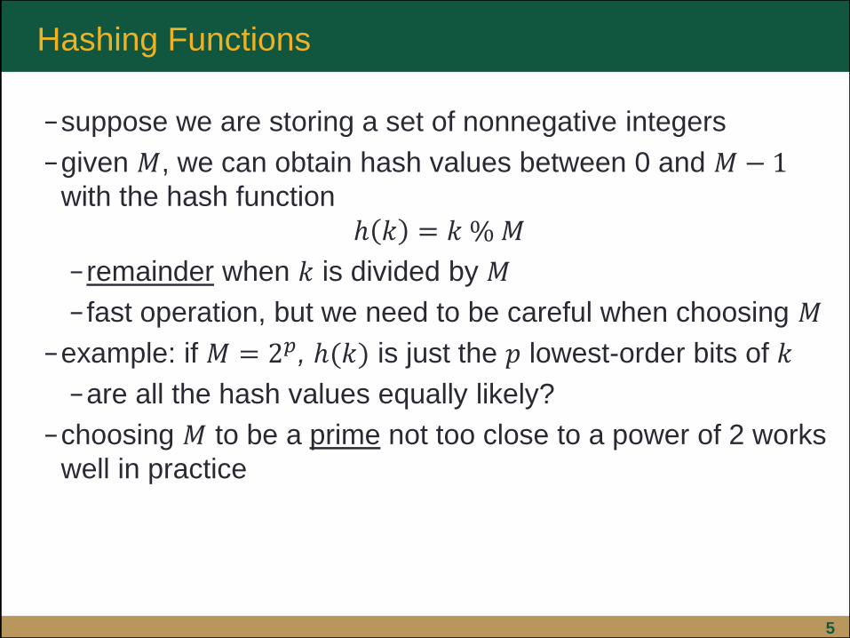
−suppose we are storing a set of nonnegative integers
−given 𝑀, we can obtain hash values between 0 and 𝑀 − 1
with the hash function
ℎ 𝑘 = 𝑘 % 𝑀
− remainder when 𝑘 is divided by 𝑀
− fast operation, but we need to be careful when choosing 𝑀
−example: if 𝑀 = 2𝑝, ℎ(𝑘) is just the 𝑝 lowest-order bits of 𝑘
−are all the hash values equally likely?
−choosing 𝑀 to be a prime not too close to a power of 2 works
well in practice

Hashing Functions
6
−we can also use the hash function below for floating point
numbers if we interpret the bits as an integer
ℎ 𝑘 = 𝑘 % 𝑀
− two ways to do this in C, assuming long int and double
types have the same length
− first method uses C pointers to accomplish this task
unsigned long *k;
double x;
k = (unsigned long *) &x;
long int hash = k % M;

Hashing Functions
7
−we can also use the hash function below for floating point
numbers if we interpret the bits as an integer (cont.)
−second uses a union, which is a variable that can hold
objects of different types and sizes
union {
long int k;
double x;
} u;
u.x = 3.1416;
long int hash = u.k % M;

Hashing Functions
8
−we can hash strings by combining a hash of each character
char *s = "hello!";
unsigned long hash = 0;
for (int i = 0; i < strlen(s); i++) {
unsigned char w = s[i];
hash = (R * hash + w) % M;
}
−𝑅 is an additional parameter we get to choose
− if 𝑅 is larger than any character value, then this approach is
what you would obtain if you treated the string as a base-𝑅
integer
Hashing Functions
9
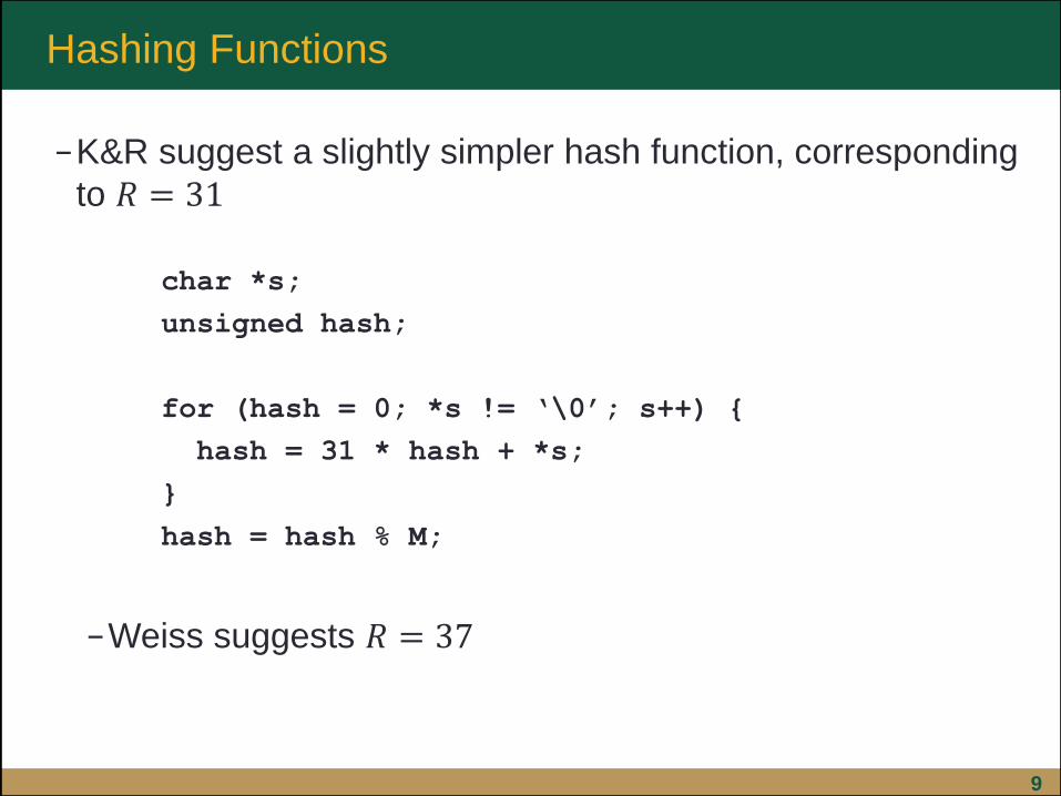
−K&R suggest a slightly simpler hash function, corresponding
to 𝑅 = 31
char *s;
unsigned hash;
for (hash = 0; *s != ‘\0’; s++) {
hash = 31 * hash + *s;
}
hash = hash % M;
−Weiss suggests 𝑅 = 37

Hashing Functions
10
−we can use the idea for strings if our search key has multiple
parts, say, street, city, state:
hash = ((street * R + city) % M) * R + state) % M;
−same ideas apply to hashing vectors
Hash Functions
11
− the choice of parameters can have a dramatic effect on the
results of hashing
−compare the text string’s hashing algorithm for different
pairs of 𝑅 and 𝑀
−plot histograms of the number of words hashed to each
hash table location; we use the American dictionary from
the aspell program as data (305,089 words)

Hash Functions
12
−example: 𝑅 = 31, 𝑀 = 1024
−good: words are evenly distributed

Hash Functions
13
−example: 𝑅 = 32, 𝑀 = 1024
−very bad

Hash Functions
14
−example: 𝑅 = 31, 𝑀 = 1000
−better

Hash Functions
15
−example: 𝑅 = 32,𝑀 = 1000
−bad

Collision Resolution
16
−hash table collision
−occurs when elements hash to the same location in the
table
−various strategies for dealing with collision
−separate chaining
−open addressing
− linear probing
−other methods

Separate Chaining
17
−separate chaining
−keep a list of all elements that hash to the same location
−each location in the hash table is a linked list
−example: first 10 squares

Separate Chaining
18
− insert, search, delete in lists
−all proportional to length of linked list
− insert
−new elements can be inserted at head of list
−duplicates can increment counter
−other structures could be used instead of lists
−binary search tree
−another hash table
− linked lists good if table is large and hash function is good

Separate Chaining
19
−how long are the linked lists in a hash table?
−expected value: 𝑁 𝑀 where 𝑁 is the number of keys
and 𝑀 is the size of the table
− is it reasonable to assume the hash table would exhibit
this behavior?
− load factor λ = 𝑁 𝑀
−average length of a list = λ
−time to search: constant time to evaluate the hash
function + time to traverse the list
−unsuccessful search: 1 + λ
−successful search: 1 + λ 2

Separate Chaining
20
−observations
− load factor more important than table size
−general rule: make the table as large as the number of
elements to be stored, λ ≈ 1
−keep table size prime to ensure good distribution

Separate Chaining
21
−declaration of hash structure

Separate Chaining
22
−hash member function

Separate Chaining
23
− routines for separate chaining

Separate Chaining
24
− routines for separate chaining

Open Addressing
25
− linked lists incur extra costs
− time to allocate space for new cells
−effort and complexity of defining second data structure
−a different collision strategy involves placing colliding keys in nearby empty slots
− if a collision occurs, try successive cells until an empty one is found
−bigger table size needed with 𝑀 > 𝑁
− load factor should be below λ = 0.5
− three common strategies
− linear probing
−quadratic probing
−double hashing

Linear Probing
26
− linear probing insert operation
−when 𝑘 is hashed, if slot ℎ 𝑘 is open, place 𝑘 there
− if there is a collision, then start looking for an empty slot
starting with location ℎ 𝑘 + 1 in the hash table, and
proceed linearly through ℎ 𝑘 + 2,…, 𝑚 − 1, 0, 1, 2, …,
ℎ 𝑘 − 1 wrapping around the hash table, looking for an
empty slot
−search operation is similar
−checking whether a table entry is vacant (or is one we
seek) is called a probe

Linear Probing
27
−example: add 89, 18, 49, 58, 69 with ℎ 𝑘 = 𝑘 % 10 and
𝑓 𝑖 = 𝑖

Linear Probing
28
−as long as the table is not full, a vacant cell can be found
−but time to locate an empty cell can become large
−blocks of occupied cells results in primary clustering
−deleting entries leaves holes
−some entries may no longer be found
−may require moving many other entries
−expected number of probes
− for search hits: ~1
21 +
1
1−λ
− for insertion and search misses: ~1
21 +
1
1−λ 2
− for λ = 0.5, these values are 3 2 and 5 2 , respectively
Linear Probing
29
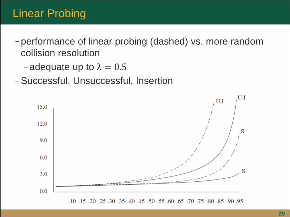
−performance of linear probing (dashed) vs. more random
collision resolution
−adequate up to λ = 0.5
−Successful, Unsuccessful, Insertion
Quadratic Probing
30
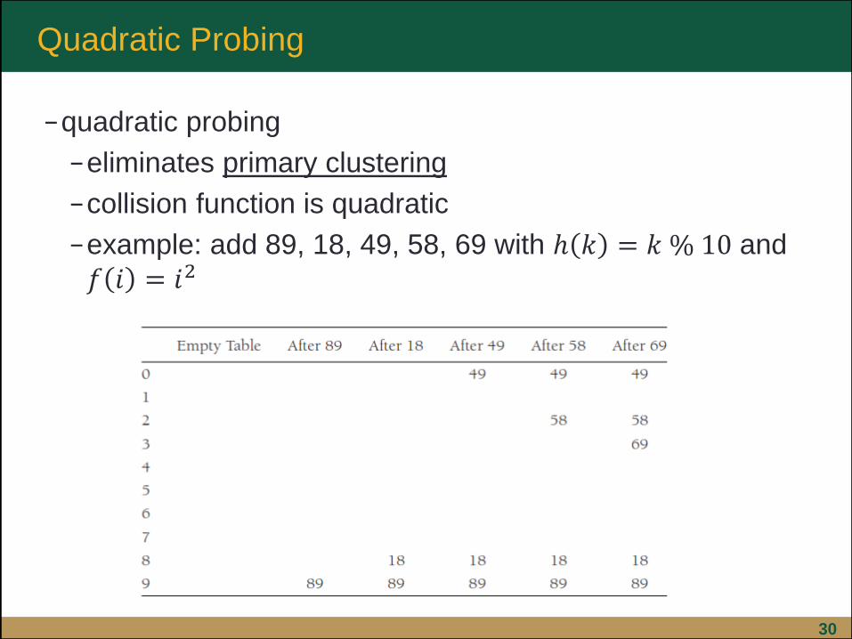
−quadratic probing
−eliminates primary clustering
−collision function is quadratic
−example: add 89, 18, 49, 58, 69 with ℎ 𝑘 = 𝑘 % 10 and
𝑓 𝑖 = 𝑖2

Quadratic Probing
31
− in linear probing, letting table get nearly full greatly hurts
performance
−quadratic probing
−no guarantee of finding an empty cell once the table gets
larger than half full
−at most, half of the table can be used to resolve
collisions
− if table is half empty and the table size is prime, then we
are always guaranteed to accommodate a new element
−could end up with situation where all keys map to the
same table location

Quadratic Probing
32
−quadratic probing
−collisions will probe the same alternative cells
−secondary clustering
−causes less than half an extra probe per search

Double Hashing
33
−double hashing
−𝑓 𝑖 = 𝑖 ∙ ℎ𝑎𝑠ℎ2 𝑥
−apply a second hash function to 𝑥 and probe across
longer distances
− function must never evaluate to 0
−make sure all cells can be probed
Double Hashing
34
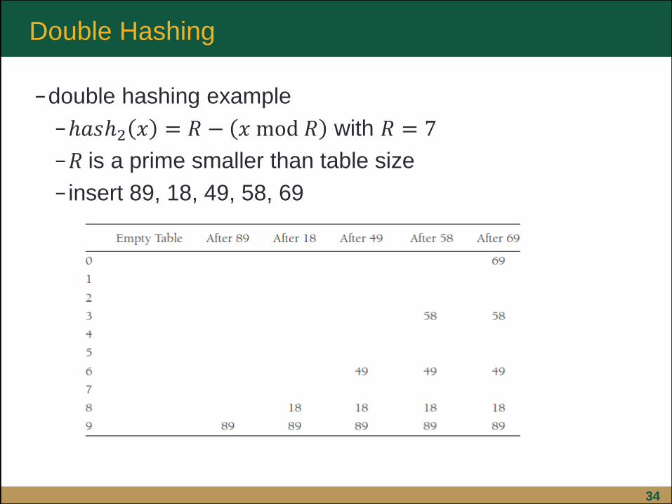
−double hashing example
−ℎ𝑎𝑠ℎ2 𝑥 = 𝑅 − 𝑥 mod 𝑅 with 𝑅 = 7
−𝑅 is a prime smaller than table size
− insert 89, 18, 49, 58, 69

Double Hashing
35
−double hashing example (cont.)
−note here that the size of the table (10) is not prime
− if 23 inserted in the table, it would collide with 58
−since ℎ𝑎𝑠ℎ2 23 = 7 − 2 = 5 and the table size is 10,
only one alternative location, which is taken

Rehashing
36
− table may get too full
− run time of operations may take too long
− insertions may fail for quadratic resolution
−too many removals may be intermixed with insertions
−solution: build a new table twice as big (with a new hash
function)
−go through original hash table to compute a hash value
for each (non-deleted) element
− insert it into the new table

Rehashing
37
−example: insert 13, 15, 24, 6 into a hash table of size 7
−with ℎ 𝑘 = 𝑘 % 7

Rehashing
38
−example (cont.)
− insert 23
− table will be over 70% full; therefore, a new table is
created

Rehashing
39
−example (cont.)
−new table is size 17
−new hash function ℎ 𝑘 = 𝑘 % 17
−all old elements are inserted into new
table

Rehashing
40
− rehashing run time 𝑂 𝑁 since 𝑁 elements and to rehash
the entire table of size roughly 2𝑁
−must have been 𝑁 2 insertions since last rehash
− rehashing may run OK if in background
− if interactive session, rehashing operation could produce
a slowdown
− rehashing can be implemented with quadratic probing
−could rehash as soon as the table is half full
−could rehash only when an insertion fails
−could rehash only when a certain load factor is reached
−may be best, as performance degrades as load factor
increases

Hash Tables with Worst-Case 𝑂(1) Access
41
−hash tables so far
−𝑂(1) average case for insertions, searches, and
deletions
−separate chaining: worst case ϴ log𝑁 log log𝑁
−some queries will take nearly logarithmic time
−worst-case 𝑂(1) time would be better
− important for applications such as lookup tables for
routers and memory caches
− if 𝑁 is known in advance, and elements can be
rearranged, worst-case 𝑂(1) time is achievable
Hash Tables with Worst-Case 𝑂(1) Access
42
−perfect hashing
−assume all 𝑁 items known in advance
−separate chaining
− if the number of lists continually increases, the lists will become shorter and shorter
−with enough lists, high probability of no collisions
−two problems
−number of lists might be unreasonably large
−the hashing might still be unfortunate
−𝑀 can be made large enough to have probability 1
2
of no collisions
−if collision detected, clear table and try again with a different hash function (at most done 2 times)

Hash Tables with Worst-Case 𝑂(1) Access
43
−perfect hashing (cont.)
−how large must 𝑀 be?
−theoretically, 𝑀 should be 𝑁2, which is impractical
−solution: use 𝑁 lists
−resolve collisions by using hash tables instead of
linked lists
−each of these lists can have 𝑛2 elements
−each secondary hash table will use a different hash
function until it is collision-free
−can also perform similar operation for primary hash
table
− total size of secondary hash tables is at most 2𝑁

Hash Tables with Worst-Case 𝑂(1) Access
44
−perfect hashing (cont.)
−example: slots 1, 3, 5, 7 empty; slots 0, 4, 8 have 1
element each; slots 2, 6 have 2 elements each; slot 9
has 3 elements

Hash Tables with Worst-Case 𝑂(1) Access
45
−cuckoo hashing
−ϴ log𝑁 log log𝑁 bound known for a long time
− researchers surprised in 1990s to learn that if one of two
tables were randomly chosen as items were inserted,
the size of the largest list would be ϴ log log𝑁 , which is
significantly smaller
−main idea: use 2 tables
−neither more than half full
−use a separate hash function for each
− item will be stored in one of these two locations
−collisions resolved by displacing elements

Hash Tables with Worst-Case 𝑂(1) Access
46
−cuckoo hashing (cont.)
−example: 6 items; 2 tables of size 5; each table has
randomly chosen hash function
−A can be placed at position 0 in Table 1 or position 2 in
Table 2
−a search therefore requires at most 2 table accesses in
this example
− item deletion is trivial

Hash Tables with Worst-Case 𝑂(1) Access
47
−cuckoo hashing (cont.)
− insertion
−ensure item is not already in one of the tables
−use first hash function and if first table location is
empty, insert there
− if location in first table is occupied
−displace element there and place current item in
correct position in first table
−displaced element goes to its alternate hash position
in the second table
Hash Tables with Worst-Case 𝑂(1) Access
48
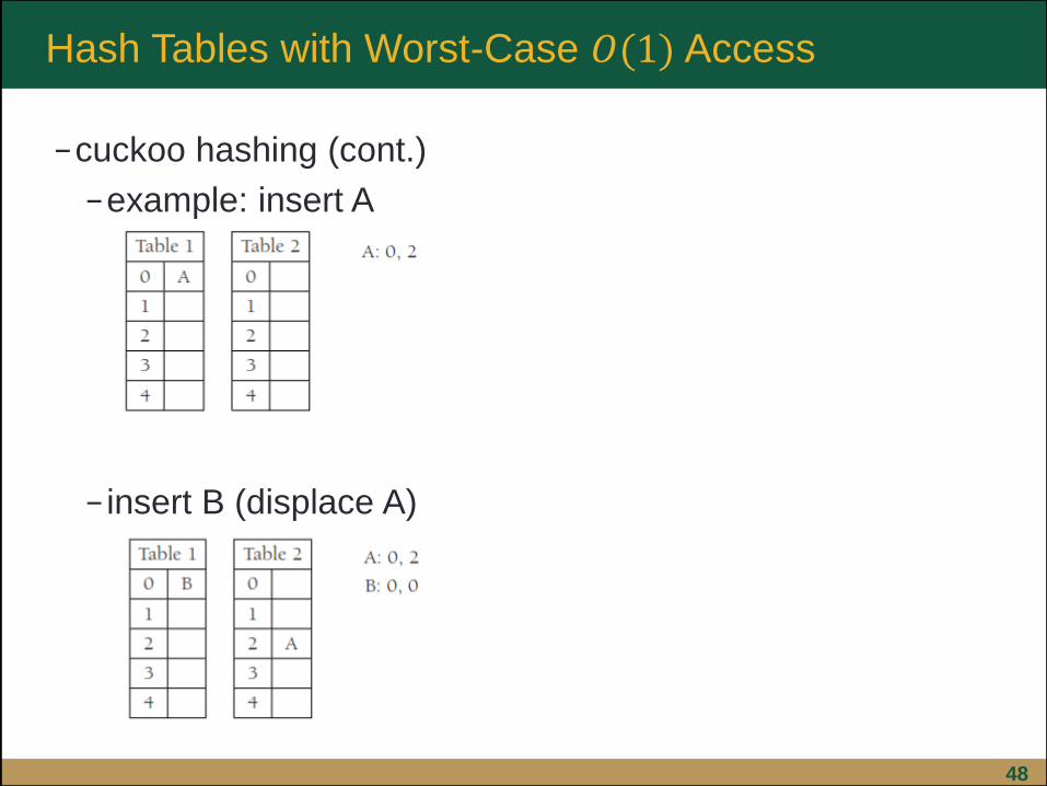
−cuckoo hashing (cont.)
−example: insert A
− insert B (displace A)

Hash Tables with Worst-Case 𝑂(1) Access
49
−cuckoo hashing (cont.)
− insert C
− insert D (displace C) and E

Hash Tables with Worst-Case 𝑂(1) Access
50
−cuckoo hashing (cont.)
− insert F (displace E) – (E displaces A)
− (A displaces B) – (B relocated)

Hash Tables with Worst-Case 𝑂(1) Access
51
−cuckoo hashing (cont.)
− insert G
−displacements are cyclical
−G D B A E F C G
−can try G’s second hash value in second table, but it
also results in a displacement cycle

Hash Tables with Worst-Case 𝑂(1) Access
52
−cuckoo hashing (cont.)
−cycles
− if table’s load value < 0.5, probability of a cycle is very
low
−insertions should require < 𝑂 log𝑁 displacements
− if a certain number of displacements is reached on an
insertion, tables can be rebuilt with new hash functions

Hash Tables with Worst-Case 𝑂(1) Access
53
−cuckoo hashing (cont.)
−variations
−higher number of tables (3 or 4)
−place item in second hash slot immediately instead of
displacing other items
−allow each cell to store multiple keys
−space utilization increased

Hash Tables with Worst-Case 𝑂(1) Access
54
−cuckoo hashing (cont.)
−benefits
−worst-case constant lookup and deletion times
−avoidance of lazy deletion
−potential for parallelism
−potential issues
−extremely sensitive to choice of hash functions
−time for insertion increases rapidly as load factor
approaches 0.5
Hash Tables with Worst-Case 𝑂(1) Access
55
−hopscotch hashing
− improves on linear probing algorithm
− linear probing tries cells in sequential order, starting
from hash location, which can be long due to primary
and secondary clustering
− instead, hopscotch hashing places a bound on
maximal length of the probe sequence
−results in worst-case constant-time lookup
−can be parallelized

Hash Tables with Worst-Case 𝑂(1) Access
56
−hopscotch hashing (cont.)
− if insertion would place an element too far from its
hash location, go backward and evict other elements
−evicted elements cannot be placed farther than the
maximal length
−each position in the table contains information about
the current element inhabiting it, plus others that hash
to it

Hash Tables with Worst-Case 𝑂(1) Access
57
−hopscotch hashing (cont.)
−example: MAX_DIST = 4
−each bit string provides 1 bit of information about the
current position and the next 3 that follow
−1: item hashes to current location; 0: no

Hash Tables with Worst-Case 𝑂(1) Access
58
−hopscotch hashing (cont.)
−example: insert H in 9
−try in position 13, but too far, so try candidates for eviction (10, 11, 12)
−evict G in 11

Hash Tables with Worst-Case 𝑂(1) Access
59
−hopscotch hashing (cont.)
−example: insert I in 6
−position 14 too far, so try positions 11, 12, 13
−G can move down one
−position 13 still too far; F can move down one

Hash Tables with Worst-Case 𝑂(1) Access
60
−hopscotch hashing (cont.)
−example: insert I in 6
−position 12 still too far, so try positions 9, 10, 11
−B can move down three
−now slot is open for I, fourth from 6

Hash Tables with Worst-Case 𝑂(1) Access
61
−universal hashing
− in principle, we can end up with a situation where all of
our keys are hashed to the same location in the hash
table (bad)
−more realistically, we could choose a hash function
that does not evenly distribute the keys
−to avoid this, we can choose the hash function
randomly so that it is independent of the keys being
stored
−yields provably good performance on average

Hash Tables with Worst-Case 𝑂(1) Access
62
−universal hashing (cont.)
− let 𝐻 be a finite collection of hash functions mapping
our set of keys 𝐾 to the range {0,1,…, 𝑀 − 1}
−𝐻 is a universal collection if for each pair of distinct
keys 𝑘, 𝑙 ∈ 𝐾, the number of hash functions ℎ ∈ 𝐻 for
which ℎ 𝑘 = ℎ(𝑙) is at most 𝐻 /𝑀
−that is, with a randomly selected hash function ℎ ∈ 𝐻,
the chance of a collision between distinct 𝑘 and 𝑙 is not
more than the probability 1 𝑀 of a collision if ℎ 𝑘
and ℎ 𝑙 were chosen randomly and independently
from {0,1,…, 𝑀 − 1}

Hash Tables with Worst-Case 𝑂(1) Access
63
−universal hashing (cont.)
−example: choose a prime 𝑝 sufficiently large that every
key 𝑘 is in the range 0 to 𝑝 − 1 (inclusive)
− let 𝐴 = 0, 1,… , 𝑝 − 1 and 𝐵 = 1,… , 𝑝 − 1
then the family
ℎ𝑎,𝑏 𝑘 = 𝑎𝑘 + 𝑏 𝑚𝑜𝑑 𝑝 𝑚𝑜𝑑 𝑀 𝑎 ∈ 𝐴, 𝑏 ∈ 𝐵
is a universal class of hash functions

Hash Tables with Worst-Case 𝑂(1) Access
64
−extendible hashing
−amount of data too large to fit in memory
−main consideration is then the number of disk
accesses
−assume we need to store 𝑁 records and 𝑀 = 4
records fit in one disk block
−current problems
−if probing or separate chaining is used, collisions
could cause several blocks to be examined during a
search
−rehashing would be expensive in this case

Hash Tables with Worst-Case 𝑂(1) Access
65
−extendible hashing (cont.)
−allows search to be performed in 2 disk accesses
−insertions require a bit more
−use B-tree
−as 𝑀 increases, height of B-tree decreases
−could make height = 1, but multi-way branching
would be extremely high
Hash Tables with Worst-Case 𝑂(1) Access
66
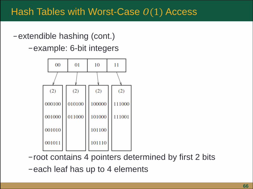
−extendible hashing (cont.)
−example: 6-bit integers
−root contains 4 pointers determined by first 2 bits
−each leaf has up to 4 elements
Hash Tables with Worst-Case 𝑂(1) Access
67
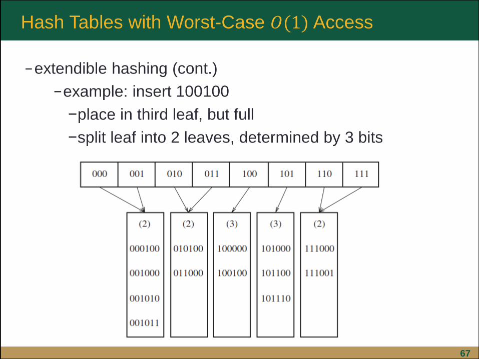
−extendible hashing (cont.)
−example: insert 100100
−place in third leaf, but full
−split leaf into 2 leaves, determined by 3 bits

Hash Tables with Worst-Case 𝑂(1) Access
68
−extendible hashing (cont.)
−example: insert 000000
−first leaf split

Hash Tables with Worst-Case 𝑂(1) Access
69
−extendible hashing (cont.)
−considerations
−several directory splits may be required if the
elements in a leaf agree in more than D+1 leading
bits
−number of bits to distinguish bit strings
−does not work well with duplicates ( > 𝑀 duplicates:
does not work at all)
Hash Tables with Worst-Case 𝑂(1) Access
70
− final points
−choose hash function carefully
−watch load factor
−separate chaining: close to 1
−probe hashing: 0.5
−hash tables have some limitations
−not possible to find min/max
−not possible to search for a string unless the exact
string is known
−binary search trees can do this, and 𝑂(log𝑁) is only
slightly worse than 𝑂(1)

Hash Tables with Worst-Case 𝑂(1) Access
71
− final points (cont.)
−hash tables good for
−symbol table
−gaming
−remembering locations to avoid recomputing
through transposition table
−spell checkers