chapter 5 – visualization 5.1 overview techniques for ... · chapter 5 – visualization...
TRANSCRIPT

© 2006 Burkhard Wuensche http://www.cs.auckland.ac.nz/~burkhard Slide 1
Chapter 5 – Visualization Techniques for Scalar Fields5.1 Overview5.2 Colour Mapping5.3 Height Fields5.4 Quick View Techniques5.5 “Marching Cubes” Algorithm5.6 Direct Volume Rendering 5.7 References
© 2006 Burkhard Wuensche http://www.cs.auckland.ac.nz/~burkhard Slide 2
5.1 Overview
Scalar data can be defined asContinuous field f(x,y,z) - defined for all (x,y,z)
Usually obtained as solution to a mathematically problem or by interpolating sampled data
Sampled volume data fijk - defined only at particular points (xi,yj,zk)
Most commonly on a cartesian gridSample values are called voxelsA cuboidal region with voxels at all 8 vertices is called a cell
Cell
Voxel
© 2006 Burkhard Wuensche http://www.cs.auckland.ac.nz/~burkhard Slide 3
Suitability of Visual Attributes for Displaying Quantitative Information
Highest accuracy of representation Position on scale
Interval length
Slope/angle
Area
Volume
ColourLowest accuracy of representation
0.0 1.0
© 2006 Burkhard Wuensche http://www.cs.auckland.ac.nz/~burkhard Slide 4
Visualisation MethodsColour mapping
Associate scalar field values with coloursVisualizes field over a surfacePerception of qualitative information limited
"Quick look" techniquesEasy to program & fast to computeWeak visualization
Surface-fitting methodsDefine surface(s) of constant field values f(x,y,z)=cCalled iso-level or iso-value surfaces, often abbreviated to isosurfacesChoose "interesting" values (isosurface levels)
e.g. between soft tissue and bone
© 2006 Burkhard Wuensche http://www.cs.auckland.ac.nz/~burkhard Slide 5
Visualization Methods (cont’d)
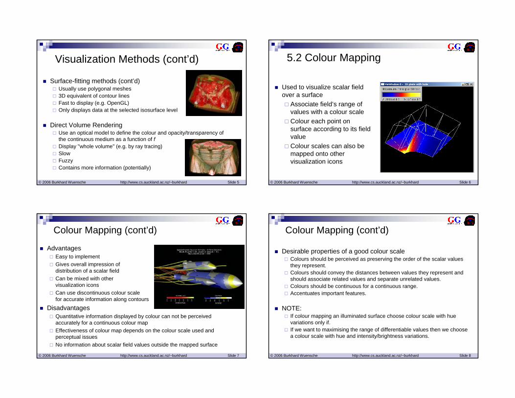
Surface-fitting methods (cont’d)Usually use polygonal meshes3D equivalent of contour linesFast to display (e.g. OpenGL)Only displays data at the selected isosurface level
Direct Volume RenderingUse an optical model to define the colour and opacity/transparency of the continuous medium as a function of fDisplay "whole volume" (e.g. by ray tracing)SlowFuzzyContains more information (potentially)
© 2006 Burkhard Wuensche http://www.cs.auckland.ac.nz/~burkhard Slide 6
5.2 Colour Mapping
Used to visualize scalar field over a surface
Associate field’s range of values with a colour scaleColour each point on surface according to its field valueColour scales can also be mapped onto other visualization icons
© 2006 Burkhard Wuensche http://www.cs.auckland.ac.nz/~burkhard Slide 7
Colour Mapping (cont’d)
AdvantagesEasy to implementGives overall impression of distribution of a scalar fieldCan be mixed with other visualization iconsCan use discontinuous colour scale for accurate information along contours
DisadvantagesQuantitative information displayed by colour can not be perceived accurately for a continuous colour mapEffectiveness of colour map depends on the colour scale used and perceptual issuesNo information about scalar field values outside the mapped surface
© 2006 Burkhard Wuensche http://www.cs.auckland.ac.nz/~burkhard Slide 8
Colour Mapping (cont’d)
Desirable properties of a good colour scaleColours should be perceived as preserving the order of the scalar values they represent.Colours should convey the distances between values they represent and should associate related values and separate unrelated values.Colours should be continuous for a continuous range.Accentuates important features.
NOTE:If colour mapping an illuminated surface choose colour scale with hue variations only if.If we want to maximising the range of differentiable values then we choose a colour scale with hue and intensity/brightness variations.

© 2006 Burkhard Wuensche http://www.cs.auckland.ac.nz/~burkhard Slide 9
Colour Mapping (cont’d)Common colour scales
E.g. H. Levkowitz and G. T. Herman. Colour scales for image data. IEEE Computer Graphics & Applicatios, 12(1):72-80, January 1992.
© 2006 Burkhard Wuensche http://www.cs.auckland.ac.nz/~burkhard Slide 10
Colour Mapping (cont’d)
Implemented using Gouraud shaded polygons (a) or 1D texture maps (b).
© 2006 Burkhard Wuensche http://www.cs.auckland.ac.nz/~burkhard Slide 11
5.3 Height Fields
Used to visualize a field over a (planar) surface
Visualize field’s values over the surface by constructing an offset surface.Height of offset surface at each point proportional to the field value at that point.Can colour map the height field to encode additional information.
© 2006 Burkhard Wuensche http://www.cs.auckland.ac.nz/~burkhard Slide 12
Height Fields (cont’d)Advantages
Accurate display of quantitative informationCan be colour mapped to display several scalar fields simultaneously – good for displaying correlation
DisadvantagesWorks best for planar surfaces.For curved surfaces height values difficult to perceive and offset surface might self-intersect Requires a large amount of screen space - might interfere with other visualization iconsOften not obvious for which surface the scalar field is visualizedNo information about scalar field values outside the mapped surface

© 2006 Burkhard Wuensche http://www.cs.auckland.ac.nz/~burkhard Slide 13
5.4 Quick-look TechniquesSlicing
May just display as images slices along coordinate axesBetter to allow arbitrary slicing planePerhaps animate motion of slicing plane to improve visualization
Wire-frame contoursTake the sampled data in slicesCompute iso-value contours in the slice planesDisplay those contours as lines in 3 spacePossibly do on more than one axisIs a simple example of "surface fitting"
© 2006 Burkhard Wuensche http://www.cs.auckland.ac.nz/~burkhard Slide 14
Surface FittingIs just contouring in 3D
Contours are now surfacesEasiest method – "Opaque Cubes"
For each cell in the volume
If cell's voxel values encompass the isolevel then Display the cell as a solid cube
Is really another "quick look" methodBuilds "Lego" approximation to object
© 2006 Burkhard Wuensche http://www.cs.auckland.ac.nz/~burkhard Slide 15
5.5 “Marching Cubes” Algorithm
Approximates isosurface through each cell with a set of polygons
Low resolution mesh Low resolution mesh rendered as Gouraud
shaded surface
High resolution mesh rendered as Gouraud
shaded surface
© 2006 Burkhard Wuensche http://www.cs.auckland.ac.nz/~burkhard Slide 16
“Marching Cubes” Algorithm (cont’d)
Easy in principleFor each cubical cellFor each edge of cellIf endpoint voxel values encompass the isosurfacevalue determine the intersection point
Connect all intersection points in cell to give one or more polygons representing surface through cell
Can make it fast by building look-up table of all possible cell configurationsEasier to understand by doing 2D case first
© 2006 Burkhard Wuensche http://www.cs.auckland.ac.nz/~burkhard Slide 17
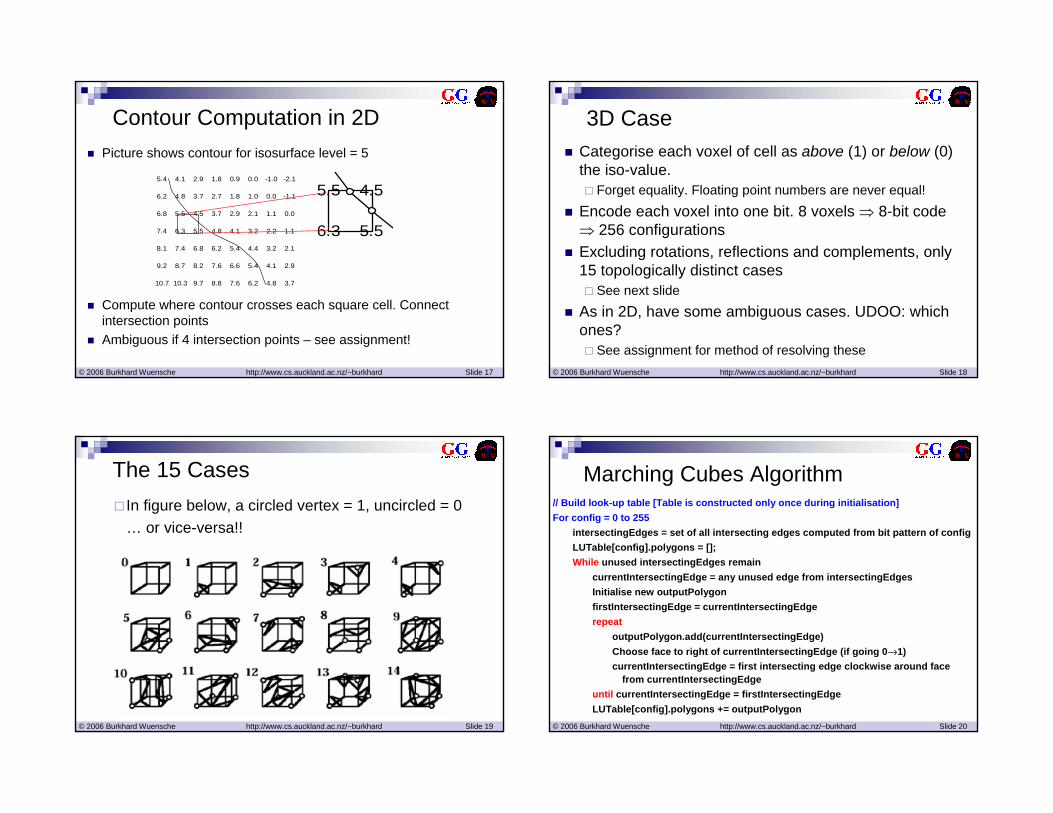
Contour Computation in 2DPicture shows contour for isosurface level = 5
Compute where contour crosses each square cell. Connect intersection pointsAmbiguous if 4 intersection points – see assignment!
5.4 4.1 2.9 1.8 0.9 0.0 -1.0 -2.1
6.2 4.8 3.7 2.7 1.8 1.0 0.0 -1.1
6.8 5.5 4.5 3.7 2.9 2.1 1.1 0.0
7.4 6.3 5.5 4.8 4.1 3.2 2.2 1.1
8.1 7.4 6.8 6.2 5.4 4.4 3.2 2.1
9.2 8.7 8.2 7.6 6.6 5.4 4.1 2.9
10.7 10.3 9.7 8.8 7.6 6.2 4.8 3.7
5.5 4.5
6.3 5.5
© 2006 Burkhard Wuensche http://www.cs.auckland.ac.nz/~burkhard Slide 18
3D CaseCategorise each voxel of cell as above (1) or below (0) the iso-value.
Forget equality. Floating point numbers are never equal!Encode each voxel into one bit. 8 voxels ⇒ 8-bit code ⇒ 256 configurationsExcluding rotations, reflections and complements, only 15 topologically distinct cases
See next slideAs in 2D, have some ambiguous cases. UDOO: which ones?
See assignment for method of resolving these
© 2006 Burkhard Wuensche http://www.cs.auckland.ac.nz/~burkhard Slide 19
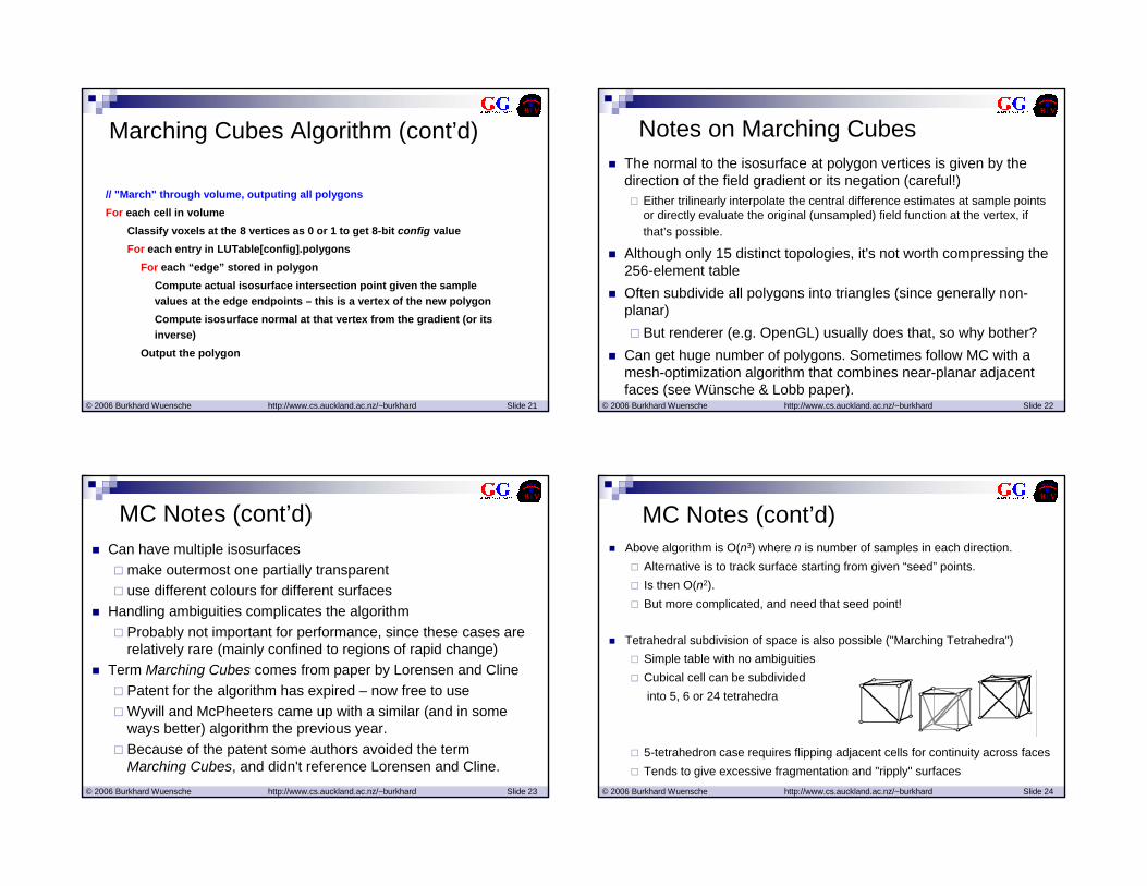
The 15 CasesIn figure below, a circled vertex = 1, uncircled = 0… or vice-versa!!
© 2006 Burkhard Wuensche http://www.cs.auckland.ac.nz/~burkhard Slide 20
Marching Cubes Algorithm// Build look-up table [Table is constructed only once during initialisation]For config = 0 to 255
intersectingEdges = set of all intersecting edges computed from bit pattern of configLUTable[config].polygons = [];While unused intersectingEdges remain
currentIntersectingEdge = any unused edge from intersectingEdgesInitialise new outputPolygonfirstIntersectingEdge = currentIntersectingEdgerepeat
outputPolygon.add(currentIntersectingEdge)Choose face to right of currentIntersectingEdge (if going 0→1)currentIntersectingEdge = first intersecting edge clockwise around face
from currentIntersectingEdgeuntil currentIntersectingEdge = firstIntersectingEdgeLUTable[config].polygons += outputPolygon
© 2006 Burkhard Wuensche http://www.cs.auckland.ac.nz/~burkhard Slide 21
Marching Cubes Algorithm (cont’d)
// "March" through volume, outputing all polygonsFor each cell in volume
Classify voxels at the 8 vertices as 0 or 1 to get 8-bit config valueFor each entry in LUTable[config].polygons
For each “edge” stored in polygonCompute actual isosurface intersection point given the sample values at the edge endpoints – this is a vertex of the new polygonCompute isosurface normal at that vertex from the gradient (or its inverse)
Output the polygon
© 2006 Burkhard Wuensche http://www.cs.auckland.ac.nz/~burkhard Slide 22
Notes on Marching CubesThe normal to the isosurface at polygon vertices is given by the direction of the field gradient or its negation (careful!)
Either trilinearly interpolate the central difference estimates at sample points or directly evaluate the original (unsampled) field function at the vertex, if that’s possible.
Although only 15 distinct topologies, it's not worth compressing the 256-element tableOften subdivide all polygons into triangles (since generally non-planar)
But renderer (e.g. OpenGL) usually does that, so why bother?Can get huge number of polygons. Sometimes follow MC with a mesh-optimization algorithm that combines near-planar adjacent faces (see Wünsche & Lobb paper).
© 2006 Burkhard Wuensche http://www.cs.auckland.ac.nz/~burkhard Slide 23
MC Notes (cont’d)Can have multiple isosurfaces
make outermost one partially transparentuse different colours for different surfaces
Handling ambiguities complicates the algorithmProbably not important for performance, since these cases are relatively rare (mainly confined to regions of rapid change)
Term Marching Cubes comes from paper by Lorensen and ClinePatent for the algorithm has expired – now free to useWyvill and McPheeters came up with a similar (and in some ways better) algorithm the previous year. Because of the patent some authors avoided the term Marching Cubes, and didn't reference Lorensen and Cline.
© 2006 Burkhard Wuensche http://www.cs.auckland.ac.nz/~burkhard Slide 24
MC Notes (cont’d)Above algorithm is O(n3) where n is number of samples in each direction.
Alternative is to track surface starting from given “seed” points. Is then O(n2). But more complicated, and need that seed point!
Tetrahedral subdivision of space is also possible ("Marching Tetrahedra")Simple table with no ambiguitiesCubical cell can be subdivided into 5, 6 or 24 tetrahedra
5-tetrahedron case requires flipping adjacent cells for continuity across facesTends to give excessive fragmentation and "ripply" surfaces

© 2006 Burkhard Wuensche http://www.cs.auckland.ac.nz/~burkhard Slide 25
Dividing CubesMarching cubes can give huge number of polygons.Can be very slow to render without special-purpose hardware –poor interactivityA faster method in such cases is Dividing Cubes. Not widely known/used.Simple idea – like opaque cubes but
recursively subdivide each cube that contains isosurface until its projection area is pixel-sized.then colour the pixel(s) it projects onto with a shade computed using a standard illumination model. Use the gradient at the centre of the cube as the surface normal.
Can get real-time frame rates on modern PCs if you're sufficiently cunning.
© 2006 Burkhard Wuensche http://www.cs.auckland.ac.nz/~burkhard Slide 26
5.6 Direct Volume Rendering
Regard scalar field values as densities of a gas-like materialGas emits light, and also attenuates light coming from behind.Let ελ be the emission per unit length along a ray for some wavelength λLet βλ be the attenuation coefficient along the ray, defined by
where Iλ is intensity.
dI Idt
λλ λβ= −
© 2003 Kitware Inc., Schroeder, Martin, Lorensen. The Visualization Toolkit
© 2006 Burkhard Wuensche http://www.cs.auckland.ac.nz/~burkhard Slide 27
The Emission-Absorption Model
Then can easily derive the emission-absorption model:
where ελdt is the light emitted by an element of the ray path, and e-thingo is the attenuation factor of the medium between the eye and the element. Iλ is just the integral over the whole ray path.Good reference: Nelson Max "Optical Models for Direct Volume Rendering", IEEE Trans. Vis. and Computer Graphics", 1(2) June 1995.
max
0
( )
0
( )
t
s
t s ds
t
I t e dtλβ
λ λε =
−
=
∫= ∫
© 2006 Burkhard Wuensche http://www.cs.auckland.ac.nz/~burkhard Slide 28
Opacity, Transparency and Colour
Papers often talk about opacity or transparency of the medium.Confusing. Defined only for a fixed distance through the medium
Usually a "slab" of the medium, i.e. the spacing between voxel slices
Transparency of a slab = Intensity Out / Intensity InSo transparency of two consecutive slabs with transparencies T1 and T2 is just T1 T2
Opacity α = 1 – Transparency
© 2006 Burkhard Wuensche http://www.cs.auckland.ac.nz/~burkhard Slide 29
Opacity, Transparency and Colour (cont’d)
UDOO: If the opacity of a 2 mm thick section of tissue in 0.8, what is the opacity of a 1mm thick section?
No, it is not 0.4.Should get 1 – Sqrt(1– 0.8) ≈ 0.55
The simple optical model assumes medium is populated with small opaque particles with emissive colour CFor a thin slab, α represents the probability that a photon will not pass through the slab.α C then represents the colour emitted by the slab (since α is a measure of "coverage")
© 2006 Burkhard Wuensche http://www.cs.auckland.ac.nz/~burkhard Slide 30
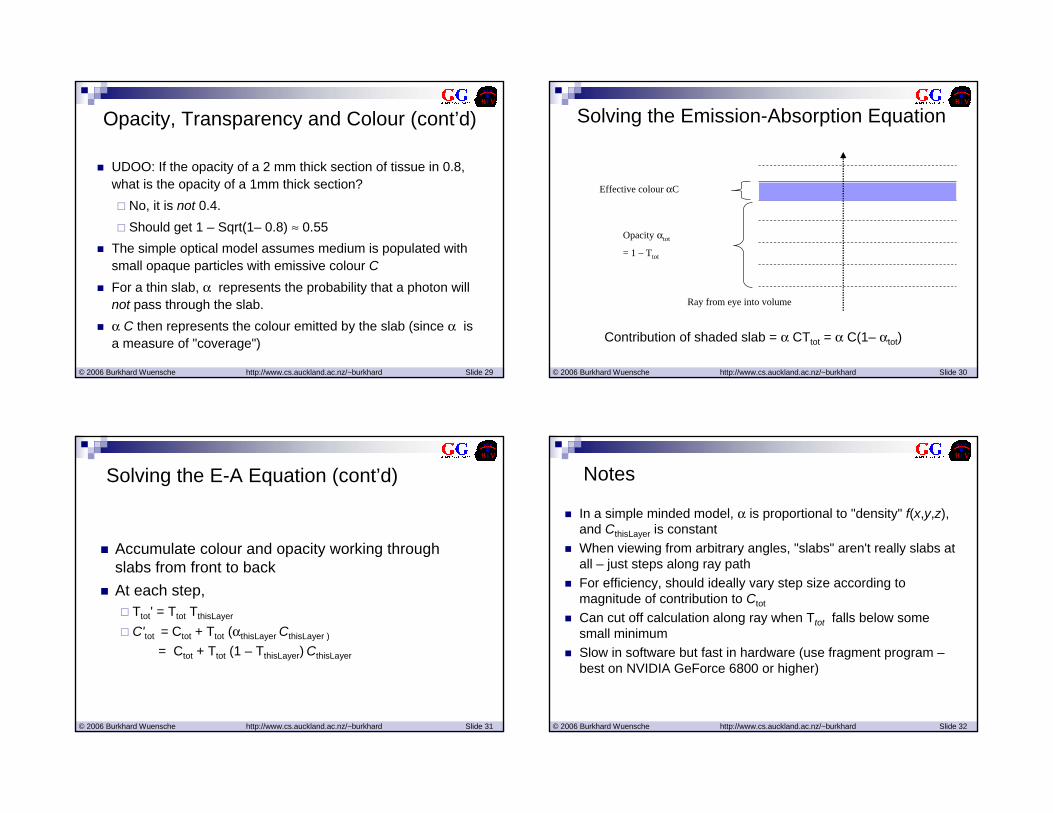
Solving the Emission-Absorption Equation
Contribution of shaded slab = α CTtot = α C(1– αtot)
Opacity αtot
= 1 – Ttot
Effective colour αC
Ray from eye into volume
© 2006 Burkhard Wuensche http://www.cs.auckland.ac.nz/~burkhard Slide 31
Solving the E-A Equation (cont’d)
Accumulate colour and opacity working through slabs from front to backAt each step,
Ttot' = Ttot TthisLayer
C'tot = Ctot + Ttot (αthisLayer CthisLayer )
= Ctot + Ttot (1 – TthisLayer) CthisLayer
© 2006 Burkhard Wuensche http://www.cs.auckland.ac.nz/~burkhard Slide 32
Notes
In a simple minded model, α is proportional to "density" f(x,y,z), and CthisLayer is constantWhen viewing from arbitrary angles, "slabs" aren't really slabs at all – just steps along ray pathFor efficiency, should ideally vary step size according to magnitude of contribution to Ctot
Can cut off calculation along ray when Ttot falls below some small minimumSlow in software but fast in hardware (use fragment program –best on NVIDIA GeForce 6800 or higher)

© 2006 Burkhard Wuensche http://www.cs.auckland.ac.nz/~burkhard Slide 33
Notes (cont’d)
Method as described so far just tends to produce a foggy mess. So:
Compute CthisLayer using a pseudo-surface reflection model, e.g. Lambert or Phong illuminationAssume some lighting configurationTake –grad f as the surface normalAlso possibly weight colour by | grad f | to emphasise high gradient regions, representing e.g. transitions between tissue types
Even with above, may still be a foggy mess unless pre-process dataset as in next slide
© 2006 Burkhard Wuensche http://www.cs.auckland.ac.nz/~burkhard Slide 34
ClassificationIf different density ranges represent different physical properties (e.g. different tissues, with CT scan), want different colours for those different rangesSo now α and C are more complex functions of density f(x,y,z)
© 2006 Burkhard Wuensche http://www.cs.auckland.ac.nz/~burkhard Slide 35
Results
© 2003 Kitware Inc., Schroeder, Martin, Lorensen. The Visualization Toolkit
Maximum Intensity projection Composite (unshaded) Composite (shaded)
© 2006 Burkhard Wuensche http://www.cs.auckland.ac.nz/~burkhard Slide 36
Direct Projection Methods
Ray tracing technique described above is an exact solution to Emission-Absorption equation.Called an “image order” method, since traverse volume one ray at a time, i.e. in an order determined by imageAlso have a range of “object order” methods, where we attempt to determine the contribution to the final image of each cell orvoxel in turn.Can do exactly ("Vbuffer algorithm" or similar) or approximately ("Splatting" algorithms).Nowadays hardware implemented methods are most common
Use 2D or 3D texture mapping

© 2006 Burkhard Wuensche http://www.cs.auckland.ac.nz/~burkhard Slide 37
GPU Based Volume Rendering
© 2004, Markus Hadwiger, Christof Rezk-Salama, Klaus Engel, Joe M. Kniss, Aaron E. Lefohn, Daniel Weiskopf, “Real-Time Volume Graphics”, ACM SIGGRAPH ’04, Course no. 28.
© 2006 Burkhard Wuensche http://www.cs.auckland.ac.nz/~burkhard Slide 38
Volume Visualization in VTK
Three steps:1. Classification
- Opacity transfer function (use vtkPiecewiseFunction)- Colour transfer function (use vtkColorTransferFunction)- Add to volume properties
2. Define a mapper (rendering technique)- Ray casting (vtkVolumeRayCastMapper and
vtkVolumeRayCastCompositeFunction)- Texture mapping (vtkVolumeTextureMapper2D)
3. Render- Add properties and mapper to the volume and add it to the render
© 2006 Burkhard Wuensche http://www.cs.auckland.ac.nz/~burkhard Slide 39
Example – Microscopy images of a sea sponge
Slice 0 Slice 1
(slices 2-37 not shown)
Slice 38 Slice 39
The resulting volume visualization with VTK
Data obtained with kind permission from the Biomedical Imaging Research Unit (BIRU), University of Auckland, New Zealand
© 2006 Burkhard Wuensche http://www.cs.auckland.ac.nz/~burkhard Slide 40
5.7 References
Marching Cubes references
Wyvill, G. and C. McPheeters, "Data structures for soft objects", The Visual Computer, 2(4), August 1986.Lorensen, W.E. & H.E. Cline, "A high-resolution 3D surface construction algorithm", Computer Graphics, 21(4):163-169, July 1987.12(10):515-526, 1996. Bloomenthal, J. "An Implicit Surface Polygonizer", in Graphics Gems IV, P324, Ed. P.S. Heckbert, Academic Press, 1994. Gives C code.Wuensche, B. "A Survey and Analysis of Common Polygonization Methods & Optimization Techniques. Machine Graphics & Vision, 6(4), 1997, pages 451-486.

© 2006 Burkhard Wuensche http://www.cs.auckland.ac.nz/~burkhard Slide 41
References (cont’d)Colour mapping references
Colin Ware. Color sequences for univariate maps: Theory, experiments, and principles. IEEE Computer Graphics & Applicatios, 8(5):41-49, September 1988.Haim Levkowitz and Gabor T. Herman. Colour scales for image data. IEEE Computer Graphics & Applicatios, 12(1):72-80, January 1992.Penny Rheingans and Chris Landreth. Perceptual principles of visualization. In Perceptual Issues in Visualization, pages 59-73, Springer Verlag, 1995.Christopher Healey, Victoria Interrante, and Penny Rheingans. Fundamental issues of visual perception for effective image generation, 1999. Course notes #6, SIGGRAPH 1999.Lawrence D. Bergman, Bernice E. Rogowitz, Lloyd A. Treinish. A rule-based tool for assisting color map selection. Proceedings of Visualization ’95, pp.118-125, 1995.
© 2006 Burkhard Wuensche http://www.cs.auckland.ac.nz/~burkhard Slide 42
References (cont’d)Volume Visualization references
Cline, H.E., Ludke, S., Lorensen, W.E., and Teeter, B.C., "A 3D Medical Imaging Research Workstation, "Volume Visualization Algorithms and Architectures, ACM SIGGRAPH ’90 Course Notes, Course no 11, ACM Press, August 1990, pp. 243-255. [This is the "Dividing Cubes" paper].Elvins, T. T., "A Survey of Algorithms for Volume Visualization," Computer Graphics, August, 1992. Volume 26, Number 3. Elvins, T.T., "Introduction to Volume Visualization: Imaging Multi-dimensional Scientific Data", ACM SIGGRAPH '94 Course # 10. M. Hadwiger, C. Rezk-Salama, K. Engel, J.M. Kniss, A.E. Lefohn, D.Weiskopf, “Real-Time Volume Graphics”, ACM SIGGRAPH ’04, Course #28, August 2004.Westover, L., "Footprint Evaluation for Volume Rendering," Computer Graphics, Vol. 24, No. 4, August 1990, pp. 367-376. [The original "splatting" paper]Kulka, P., “High-Resolution Splatting”, PhD Thesis, Univ. of Auckland, 2001