Chapter: 5Problem FormulationThis chapter provides an extended mathematical frame work for the formulatingthe problem of reconstruction for the different beam profiles along the variousapproaches to solve the problem. The results obtained after the implementation arealso discussed.5.1 Problem Formulation for Parallel Beam ScannerParallel Beam profile is most used beam profile for all generation of CT scanner.Hence, the problem for reconstruction needs to be modelled and implemented. [1,2]5.1.1. Geometry of Parallel beam ScannerFigure 5.1 shows pictorial representation of the parallel beam scanner, which is themoveable part of the scanner and is consisting of an emitter of X-rays and a screenon which radiation detectors are placed. This revolves around the body beingexamined. The detectors measure the attenuated intensity and it is evaluatedrelative to the original radiation intensity as defined in equation 3.13. This value ofprojection is represented by ( , ) where is the angle at which the projectionis carried out and is the position of a particular place on the screen.

Figure 5.1: Basic Geometry of Parallel Beam Scanner

55

This method of scanning allows obtaining the image of the attenuation coefficientdistribution for one cross-section of the body under examination. As shown in thefigure 5.2, the scanner geometry is in the plane x and y coordinates, that is in theplane perpendicular to z-axis. Using the standard definition of Radon transform [1]it can be derived:

Figure 5.2: Scanner Geometry in X-Y Plane

( , ) = (∞

∞− , sin + cos ) (5.1)

This allows easy interpretation of value at each point on the screen. The aboveequation in the frequency domain can be represented by:( , ) = { ( , )} = ( , )∞

∞(5.2)

As mentioned in equation 3.36, the practical implementation of the above problemcan be solved by using two approaches as below: Convolution and back projection method; Filtration and back projection method.

56

5.1.2. Convolution and Back projection methodOut of two approaches, reconstruction by convolution and back projection is mostpopular [3-5] due to its simplicity and its implementation. In this approach, filteringtakes place in s-domain and this can be mathematically expressed as:( , ) = ( ( , ). . ( )) (5.3)

By applying the Fourier transform, it is converted into form:( , ) = ( ( , ) ∗ ( . ) (5.4)

This will lead to: ( , ) = ( , ) ∗ ( . ) (5.5)Comparison of equation 3.36 and 5.5 will result into:

( cos + sin , ) = ( , ) ∗ ( . ) (5.6)By using Hebert transformation, it can be stated:

12 ( ̇, ) 1− ̇ ̇ = ( , ) (5.7)The values of ( , ) obtained in this process need to be subjected to the processof back-projection in order to reconstruct the final image. Mathematically, it can beexpressed as:

( , ) = ( ( , ( , ) ∗ {| |} (5.8)

57

Figure 5.3: Projection at various Angle

If it is assumed that ( , ) is a function approximating to the ( , ), then equation5.8 can be modified as:( , ) = ( ( ). 2 . ( ,∞

∞). . ( ). ). (5.9)

where is cut off frequency function. Hence, finally it can be written as:( , ) = ( , ) ∗ ℎ ( ). (5.10)

where ℎ ( ) is the point spread function of the selected convolution kernel.Considering the practical implementation, equation 5.10 needs to be converted intodiscreet form as there are limited number of projections which are carried outduring each revolution of X-ray tube and limited resolution, at which the radiationintensities are measured. The angles at which discreet projections are carried outare represented by:= Δα (5.11)

58

where = 0,… . ,Ψ − 1 and the detectors are placed at equal distance = .Δhence the index variable = − ,… , − . The equation 5.10 can beimplemented as shown in figure 5.4:

Figure 5.4: Flow chart for Convolution Back projection Method

5.1.3. Filtration and Back projection MethodIn this approach, the filtering is carried out in the frequency domain [6-8] ascontrast to s-domain in convolution approach. Applying Fourier transform toindividual projection, the equation 5.4 can be written as:( , ) = ( ( , ) . . ( ). (5.12)

So, ( cos + sin , ) = ( , ) . . ( ) (5.13)Hence, ( , ) = (| |. ( , ) (5.14)

ProjectionData

Filtration ins-domain

Backprojection

ImageReconstruction

ImageDisplay

( )Filter Form

59

Mathematically, it can be expressed as:( , ) = ( | |. ( , ) (5.15)As seen in section 5.1.2, for the limited band spectrum, we approximate ( , ) forthe function ( , ).mathematically, it can be written as:( , ) = ∞

∞( , ) ∗ ( ) ) (5.16)where ( ) is spectrum of selected convolution kernel. Hence, the sequence ofoperation to implement reconstruction algorithm can be written as:( , ) = { { ( , )}. ( )}} (5.17)For practical implementation, the above form is converted into discreet form asdiscussed in section 5.1.2 and flow chart for the implementation is shown in figure5.5.

Figure 5.5: Flow chart for Filtration Back projection Method

ProjectionData

FourierTransform

Filtration inf domain

Inverse FourierTransform

BackProjection

( )Filter Form

ImageReconstruction

ImageDisplay

60

5.2 Problem Formulation for Fan Beam ScannerOne of the major disadvantages of parallel beam scanner is the lateral movement ofthe source and detector which leads to artefacts in the reconstructed image. Thiscan be overcome by using fan beam shaped detectors array as discussed in chapter3. The reconstruction problem can be formulated on the same line as for theparallel beam scanner. Before problem formulation, it is necessary to understandthe geometry of scanner as discussed in the next section.5.2.1. Geometry of Fan beam ScannerAs the name suggests, the beam profile is in fan shaped as opposite to parallel beamas can be seen in figures 5.6. [9]

Figure 5.6: Basic shape of Fan Beam Profile

It is evident that axis of rotation of the system and the axis of symmetry of radiationbeam plays very vital role in geometrical relationship. The axis of rotation isdirected along the line perpendicular to the cross section. A ray emitted from thetube at a given angle of rotation and reaching a particular detector can be identified61

by parameter ( , ), where is the angle that the ray makes with the principalaxis of the radiation beam and is angle of rotation.As in the parallel beam, the motion of the tube detector arrangement is rotational.The angle will be in the range of [0,2 ) , and thus the corresponding range for thewill be:

= = arcsin( ) (5.18)where is the radius of the circle and is the radius of circle describing the focusof the tube. In most of cases, the lies within the range of [− , ]. The projectionfunction for the fan beam profile is mathematically represented as:

( , ) (5.19)

Figure 5.7: Basic Geometrical Relationship for Fan Beam

For the practical implementation, the problem must be addressed into the discreetdomain. Hence, the geometry of discreet projection system must be analysed. Thefan beam scanner can be divided into two broad categories; equiangular sampling62

and equidistance sampling. But, for practical reasons and due to limitation of the X-ray tube, equidistance sampling systems are widely used. In the equidistancesampling system, the projection is obtained at predetermined angles . Hence, theangular distance is determined by the location of the detectors. As the system isequidistance, the angular distance between the detectors is equal and is obtainedby Δ .The discreet angles at which projections are made can be given by:= ∆ (5.20)where ∆ is the angle through which tube screen system is rotated and =0, 1, … , Γ− 1 is the sample index for each projection. The location of the arc isdefined by an angle:

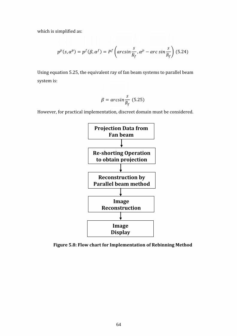
= Δ (5.21)where Δ is the distance between the radiation detector, is the index of detectormatrix. Hence, the projection value for the fan beam profile can be expressedmathematically as: ( , ) = Δ , ∆ (5.22)5.2.2 Rebinning Reconstruction MethodThis method uses re-shorting for [10-12] reconstruction of image. In this method,all the projections ( , ), which correspond to the hypothetical parallel beamprojection ( , ) are identified. The rays which would be equivalent to theparallel rays will be considered and collected. The projection data obtained willused for the reconstruction as per the methods described in section 5.1. The flowchart for the implementation of this method is shown in the figure 5.8.Mathematically, ( , ) = ( , ) = sin , + (5.23)

63

which is simplified as:( , ) = ( , ) = , − (5.24)

Using equation 5.25, the equivalent ray of fan beam systems to parallel beamsystem is:= (5.25)However, for practical implementation, discreet domain must be considered.

Figure 5.8: Flow chart for Implementation of Rebinning Method

Projection Data fromFan beam

Re-shorting Operationto obtain projection

Reconstruction byParallel beam method

ImageReconstruction

ImageDisplay

64

5.2.3 Direct Fan Beam Reconstruction MethodIn opposite to the using the reconstruction methods developed for the parallelbeam systems, here a direct approach is used to solve the problem [13,14]. Here,the formula for the parallel beam method is found in which the values obtainedfrom the fan beam can be directly used. In other words, this method can beconsidered as the extension of the parallel beam reconstruction method. Using theequation 5.5, the relationship between the quantities of two approaches can beexpressed as: = . (5.26)= + (5.27)

Converting the equation to polar form, using equation 5.26 and equation 5.27:( − ∅) − = ̇ sin( ̇ − ) (5.28)

where ̇ = arctan ( ∅ ∅ ) . The following sequence of equation based onRadon transforms can be derived:( , ) = (∞

∞

∞

∞, ). ( ) (5.29)

Converting above into polar form:( , ) = | | ( ,∞

∞). ( ) (5.30)

As the system is using fan beam profile, the limit of integration changes:( , ) = 12 | | ( ,∞

∞). ( ) (5.31)

Converting above equation 5.31 into frequency domain, it is reformulated to:65

( , ) = 12 | | ( ,∞

∞). ( ) (5.32)

As discussed in above sections, the above method can be implemented in discreetdomain. The implementation steps are shown in the figure 5.9

Figure 5.9: Flow chart for implementation of Direct Fan Beam Method

5.3 ImplementationAs discussed in previous sections most of CT scanner either uses the Parallel beamprofile or Fan beam profile. But it is evident that if scanner uses the fan beamprofile but in one form or other reconstruction problem is reformulated to parallelbeam reconstruction problem. Hence, it is logical to address parallel beamreconstruction problem and implement the same. As stated in Chapter 4,MATLAB®(R) platform is used to implement the research.In order to implement and test the reconstruction method user defined phantomwith the resolution 256X256 is used [15], the detail description is discussed inChapter 7 in detail. The user defined phantom is shown in the figure 5.10:

Projection Data fromFan beam

Direct Fan beammethod

ReconstructedImage

ImageDisplay

66

Figure 5.10: User defined Phantom.

Before applying the method discussed in previous section is interesting, to viewreconstructed image by only applying the back projection algorithm the resultobtained can be viewed in the figure 5.11:

Figure 5.11: Reconstructed User defined Phantom using Back projection

Implementing the method discussed in section 5.1.2 on the MATLAB®(R) platformthe phantom reconstructed is shown in the figure 5.12:

67

Figure 5.12: Reconstructed User defined Phantom using Convolution andBack projection

On similar lines the method discussed in section 5.1.3 the result obtained is shownin figure 5.12. From the result it can be concluded that by employing the methodsdiscussed in the chapter the quality of the image has improved significantly andthus making the diagnosis more accurate.

Figure 5.13: Reconstructed User defined Phantom using Filtration and Backprojection

68

The details analysis and comparative analysis of the results obtained by theimplementation of this work is being discussed in Chapter 8. The function files thatare developed to implement the existing techniques are listed in table 5.1:Sr.No

Name of Function File Purpose

01 ct_reconstruction It is main function file which takesrequired input from the user andproduces the output.02 phtantom_data It creates the phantom data as per thechoice of the user.02 radon It converts the generated phantomdata into projection data.03 simple_backprojection It performs back projection operationon the pre-processed image.04 filtered_backprojections_con It performs convolution operation onthe projection data05 filtered_backprojection_fd It performs filtration operation infrequency domain on projection data.

Table 5.1: Table listing the MATLAB® Function Files Developed forImplementation.

5.4 Concluding RemarksChapter discusses mathematical derivation for existing reconstruction techniquesand the step wise implementation and testing of these techniques was done onMALTLAB platform and corresponding results obtained as shown in the aboveshown figures.

69