Chapter 4 Notes and elaborations for Math 1125-Introductory Statistics

Assignment:

Chapter 4 is fairly well written, for the most part. You will want to read section 4.1, 4.2 and 4.3 very carefully.

Note that “subjective probability” as mentioned in section 4.1 isn’t mathematical probability at all and as such I

won’t be testing it.

Do the following exercises: 4.1: 1-5 all, 7, 8, 10-14, 17, 21, 23, 29, 31.

4.2: 1, 2, 3, 5, 7, 9, 15, 19.

4.3: 1, 5, 7, 21, 23, 25, 29, 31, 33, 35, 47.

This chapter introduces basic finite discrete probability theory. Most of the following material is covered in the

book, but please read through this as well. As usual, let’s start with some definitions.

______________________________

4.0 Definitions and some basic set theory

In this section, we give some basic definitions and set theory necessary for the discussion of probability.

Definition 4.0.0 The outcome of an experiment is the result of the experiment.

When you perform an experiment, you get a result. This result is an outcome. For example, if your experiment is

to roll a standard die, you will roll one of 1, 2, 3, 4, 5, or 6. Whatever you roll is the outcome of the experiment.

Definition 4.0.1 The sample space is the set of all possible outcomes of an experiment and is denoted as S.

The sample space is written as a set.

________________________________

Example 4.0.0

Your experiment is rolling a die: S = {1,2,3,4,5,6}.

Your experiment is planting ten seeds to count the number that germinate: S={0,1,2,3,4,5,6,7,8,9,10}, where the

numbers in the sample space represent the number of seeds that germinated.

Your experiment is to toss a coin three times: S ={ HHH, HHT, HTH, HTT, THH, THT, TTH, TTT}.

________________________________

By the way, there is no order in sets, e.g., {1, 4, 5} = {4, 5, 1} = {5, 1, 4}. It is important to be able to list the (basic)

outcomes clearly, for if we know all possible outcomes, determining probabilities of specific events is easy!

Definition 4.0.2 An event is a subset of the sample space.

Event are also written as sets. Before we give some examples of events, we need the concept of the empty set.

Definition 4.0.3 The empty set is a set that contains nothing and is denoted as {} or � (it depends on the author’s

preference).

Note that S is a subset of itself, and � is a subset of S, so an event can be all of S or it can be empty.

________________________________Example 4.0.1

The experiment is rolling a die. Let A be the event that the roll of a die is even. Let B be the event that the roll isgreater than 3. Let C be the event “roll greater than 7”. Let D be the event “roll a 1, or a 6, or a number between1 and 6”. Find A, B, C, and D.

A={2,4,6}, B = {4,5,6}, C = �, D = S

________________________________

Also note that an event must be well-defined. For example, the event “roll a nice number” isn’t well-definedbecause nice means different things for different people.

Definition 4.0.4 The complement of an event E is the event where E doesn’t happen.

We denote the complement of an event with a bar over the name of the event (not to be confused with notation forthe mean of a sample!).

________________________________Example 4.0.2

Suppose E={all red cars in the US}. The complement of E is E ={all cars in the US that are not red}.

From Example 4.0.1, the complement of A is A={1,3,5}, and the complement of B is B = {1,2,3}.

________________________________

Note that the complement of � is S and the complement of S is �. Some books use the notation EC instead of a

bar above.

We can build new events from old events using the and and or operators from set theory.

The event “E and F” means that both E and F happen. It’s what the two events have in common, i.e, their

intersection. Common notation for the and operator is �, the intersect symbol. We read E � F as “E intersect

F”. Notice that if S is our sample space and E is an event, then we have E � E = � and E � S = E.

The event “E or F” means that either E or F or both happen. It’s the combination of the sample spaces for both

events, i.e., their union. Common notation for the or operator is �, the union symbol. We read E � F as “E union

F”. Notice that if S is our sample space and E is an event, then E � E = S.

________________________________Example 4.0.3

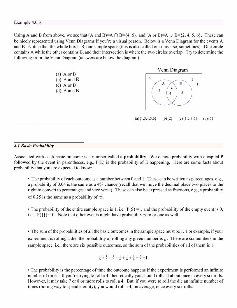
Using A and B from above, we see that (A and B)=A � B={4, 6}, and (A or B)=A � B={2, 4, 5, 6}. These can

be nicely represented using Venn Diagrams if you’re a visual person. Below is a Venn Diagram for the events Aand B. Notice that the whole box is S, our sample space (this is also called our universe, sometimes). One circlecontains A while the other contains B, and their intersection is where the two circles overlap. Try to determine thefollowing from the Venn Diagram (answers are below the diagram):

(a) A or B(b) A and B (c) A or B(d) A and B

(a){1,3,4,5,6} (b){2} (c){1,2,3,5} (d){5}

________________________________

______________________________4.1 Basic Probability

Associated with each basic outcome is a number called a probability. We denote probability with a capital Pfollowed by the event in parentheses, e.g., P(E) is the probability of E happening. Here are some facts aboutprobability that you are expected to know:

• The probability of each outcome is a number between 0 and 1. These can be written as percentages, e.g.,a probability of 0.04 is the same as a 4% chance (recall that we move the decimal place two places to theright to convert to percentages and vice versa). These can also be expressed as fractions, e.g., a probability

of 0.25 is the same as a probability of .

• The probability of the entire sample space is 1, i.e., P(S) =1, and the probability of the empty event is 0,i.e., P({}) = 0. Note that other events might have probability zero or one as well.

• The sum of the probabilities of all the basic outcomes in the sample space must be 1. For example, if your

experiment is rolling a die, the probability of rolling any given number is . There are six numbers in the

sample space, i.e., there are six possible outcomes, so the sum of the probabilities of all of them is 1:

+ + + + + = =1.

• The probability is the percentage of time the outcome happens if the experiment is performed an infinitenumber of times. If you’re trying to roll a 4, theoretically you should roll a 4 about once in every six rolls. However, it may take 7 or 8 or more rolls to roll a 4. But, if you were to roll the die an infinite number oftimes (boring way to spend eternity), you would roll a 4, on average, once every six rolls.

The probability of an event is calculated by adding up the probabilities of all the outcomes comprising the event.

For example, suppose your experiment is rolling a die. You probably know intuitively that the chance of rolling

an even number is 50% because half the numbers are even. This is given symbolically by

P({2,4,6})=P({2})+P({4})+P({6})= + + = = .

When the experiment is rolling a die, all the outcomes have equal probabilities. These are special types of

experiments.

Definition 4.1.1 Experiments where all outcomes have the same probability are called equally likely experiments.

Rolling a (fair) die is an equally likely experiment. So is drawing a single card from a deck, randomly choosing a

candy bar when there are three of each kind in a box, having a child (you have the same probability of having a boy

or a girl), etc. Equally likely experiments are very nice experiments.

The probability of an event when the experiment is equally likely is always the number of outcomes in E divided

by the number of outcomes in S, i.e.,

Equation 4.1.0 .

So, for E={roll an even number}, there are three possible outcomes in E. There are a total of six possible outcomes

in S. Thus we have P({roll an even number}) = , as we found above.

________________________________

Example 4.1.1

Suppose you have a box with three snickers, three milky ways, and two 3 musketeers. Suppose also that you can

not tell the type of candy bar by touch alone. The experiment is as follows: someone blindfolds you and you

randomly choose a candy bar from the box.

Let A={draw a snickers}, B={draw a milky way}, and C={draw a 3 musketeers}. Find the following probabilities.

(a) P(A), P(B), P(C) and (b) P(A or B), P(A or C), P(B or C)

This is an equally likely experiment! According to what’s above, we can find the probability of event A by adding

up all the probabilities comprising the event. Well, there are 3 snickers in the box and each has a 1/9 chance of

being drawn, so we get

P(A) = + + = = .

Note that there are 3 outcomes in event A and there are 9 outcomes in the sample space. Since this experiment is

an equally likely experiment, we could just use Equation 4.1.0 above to get

P(A) = = =

It should be clear that P(A) = P(B) = P(C).

To find P(A or B), we do the same thing. We add up the probabilities of all outcomes that make up the event “A

or B.” This event consists of drawing either a snickers or a milky way. Well, there are 6 outcomes in this event,

and there are 9 outcomes in the sample space. So we get

P(A or B) = = = .

And it should be clear that P(A or B) = P(A or C) = P(B or C).

________________________________

Not all experiments are equally likely so we can’t always use this formula! Here is an example of such a case.

________________________________

Example 4.1.2

Suppose your experiment is planting 5 seeds and checking two weeks after planting to see how many seeds

germinated. Our sample space is S = {0, 1, 2, 3, 4, 5}, where the numbers in the sample space represents the

number of seeds that germinated. Suppose also that we know the following probabilities:

S = s P(s)

0 .35

1 .05

2 .05

3 .25

4 .25

5 .05

So, the probability that 0 seeds germinate is .35, the probability that exactly 1 seed germinates is .05, the probability

that exactly 4 seeds germinate is .25, etc.

Use the table above to find the following probabilities:

(a) P({no more than 2 seeds germinated})

No more than two means either 0, 1, or 2 seeds germinated. This can be expressedas P({0,1,2}) and is calculated by adding the respective probabilities. So,

P({no more than 2 seeds germinated})=P({0,1,2})= .35+.05+.05 = .45.

(b) P({at least 4 seeds germinated})

At least four means either 4 or five seeds germinated. This can be expressed as

P({4,5}) = .25+.05 = .30

Notice that the complement of {4,5} is {0,1,2,3} and P({0,1,2,3}) = 1 - P({4,5}) = .70 (more on this next).

________________________________

Definition 4.1.1 Two events are said to be mutually exclusive or disjoint events if they cannot both occur together.

Consider, again, rolling a die. You cannot roll a 2 and a 4 in a single roll; the events are mutually exclusive. If A

and B are disjoint, then their intersection is empty, i.e., A �B = {}. It follows that P(A and B) = 0 if and only if

A and B are disjoint. If and only if, denoted �, means that if P(A and B) = 0, then A and B are disjoint, and if A

and B are disjoint, then P(A and B) = 0. (This is for finite discrete probability only.)

Sometimes, finding the probability of the complement of an event is less computationally tedious than calculating

the probability of the event itself. Note that for any event A, we have that A�A= S, where A and A are disjoint (an

event and its complement are disjoint by defintion). So, P(S) = P(A) +P(A). But we know P(S) = 1, so substitute1 in for P(S), do a little basic algebra, and we have the following formula for the probability of the complement

of an event:

Equation 4.1.1 P(A)=1- P(A), or equivalently, P(A) = 1-P(A).

________________________________Example 4.1.3

Consider again the experiment in Example 4.1.2. Find the probability that at least one seed germinated.

“At least one” means that 1, 2, 3, 4, or 5 seeds germinated. So, we add all the respective probabilities. However, it is much simpler to recognize that ‘at least one’ is the complement of ‘none’. So, the probabilitywe seek is given by

P({1,2,3,4,5}) = 1-P({0}) = 0.65.

Clearly, using the complement here is much easier than adding all the other probabilities.________________________________

Germinating plants

Now we are ready to find probabilities of combinations of events! We’ll start with the addition rule. Note that

the addition rule does not mean we are adding events themselves. It means we are finding the probability that the

union of the events happens.

For mutuallly exclusive events (defined above) A and B, the addition rule is

Equation 4.1.2 P(A or B) = P(A) + P(B).

Consider once more the experiment in Example 4.1.2. Let A be the event that exactly 1 seed germinates, and B be

the event that exactly 5 seeds germinate. These events are mutually exclusive, so P(A or B) = .05 +.05 = .10.

If events are not mutually exclusive, addition rule gets a little messier. Consider that when we take the union of

two events whose intersection is not empty, we are essentially counting the common outcomes twice. For example,

if we are rolling a die and A={1,2,3} and B={2,3,4}, then A�B = {1,2,3,2,3,4}={1,2,3,4}. When calculating

probabilities of union of events, we account for this ‘double counting’ by subtracting the probability of the

intersection. So, our formula becomes

Equation 4.1.3 P(A or B) = P(A) + P(B) - P(A and B).

________________________________

Example 4.1.4

Suppose our experiment is to draw one card from a standard deck of 52 cards. Find the probability of drawing a

diamond or a 5.

Symbolically, this looks like P({diamond or 5}). We know that there are 13 diamonds and four 5's in the

deck. We also know that one of the 5's is both a diamond and a 5, so there is a non-empty intersection

between the events ‘draw a diamond’ and ‘draw a 5', i.e., these are not mutually exclusive events. We must

add the probability of the events and subtract out their intersection. So, we have

P({diamond or 5}) = P({diamond })+P({5})-P({diamond and 5})

=

=

= .

________________________________

________________________________

Example 4.1.5

Instead of rolling a single die, let’s shake things up a bit and roll two dice at the same time. Suppose we are

considering the sums of the rolls, e.g., if you roll a 2 and a 4, the sum is 6. Our sample space is the shaded area of

the following table:

1 2 3 4 5 6

1 2 3 4 5 6 7

2 3 4 5 6 7 8

3 4 5 6 7 8 9

4 5 6 7 8 9 10

5 6 7 8 9 10 11

6 7 8 9 10 11 12

Each shaded cell has a probability of as each outcome is equally likely. Find the following probabilities:

(a) P(roll a sum of 8 or a sum of 5)

The events “roll a sum of 8” and “roll a sum of 5” are mutually exclusive, so we have

P({8,5}) = P({8}) + P({5}) = = .

(b) P(sum is even or sum is a multiple of 3)

The events “sum is even” and “sum is a multiple of 3” are not mutually exclusive, so we have

P({even, multiple of 3}) = P({even}) + P({multiple of 3}) - P({even and multiple of 3})

=

= .

________________________________

Now we move on to somewhat trickier stuff.

______________________________

4.2 Conditional Probability

Conditional probability is denoted P(A|B) and it is the probability of A given that B has already happened or will

happen before A. Sometimes common sense or intuition will easily provide the answer to these types of problems.

The trick to seeing conditional probability is that, if we know that we’re conditioning on B, then we simply reduce

the sample space to only the outcomes in B (because B has already happened, or will happen before A). Following

are pictures of what we just stated.

Here’s the original picture:

Here’s the picture using the knowledge that B will happen or has already happened:

So, when we say the probability of A given B, we mean we want the shaded area in the following diagram:

Provided that P(B) is not zero, the formula is

Equation 4.2.0 P(A|B) = ,

i.e., the probability of A given B is the probability of both A and B happening divided by the probability of B. As

stated previously, many times, intuition will help us find conditional probabilities.

________________________________

Example 4.2.0

Consider the experiment of Example 4.1.5. Let A be the event that we roll an even sum, and let B be the event that

we roll a sum of 6. Find the following conditional probabilities:

(a) P(A|B)

This is the probability of A given that B happened. Our intuition will work just fine here since we’re

considering the probability of rolling an even sum given that we’ve already rolled a 6. We know this

probability is 1 because 6 is an even number. However, let’s employ the formula for kicks! So we

need to find P(A and B) and P(B). We have

P(A and B) = P(sum is even and sum is 6) = P(sum is 6) = P(B).

Thus, we have P(A|B) = P(A and B) / P(B) = P(B) / P(B) = 1.

(b) P(B|A)

This is different. We’re looking for the probability of B given that A has happened. So, we need

to find the probability we rolled a sum of 6 given that we’ve rolled an even sum. This is not

intuitively clear. So, we must use the formula. Notice that we are conditioning on A, so P(A) will

be our denominator. Like before, we have

P(A and B) = P(sum is even and sum is 6) = P(sum is 6) = P(B) = .

We also have that P(A) = . So, employing the formula, we get

P(B|A) = P(A and B) / P(A) = / = * = .

Checking with the table from the example, we see that 18 outcomes are even numbers, and of those,

5 are the number 6. So, given that we’ve rolled an even number, the probability of it being a 6 is

5/18.

________________________________

________________________________

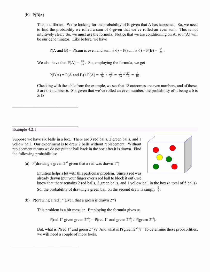
Example 4.2.1

Suppose we have six balls in a box. There are 3 red balls, 2 green balls, and 1

yellow ball. Our experiment is to draw 2 balls without replacement. Without

replacement means we do not put the ball back in the box after it is drawn. Find

the following probabilities:

(a) P(drawing a green 2nd given that a red was drawn 1st)

Intuition helps a lot with this particular problem. Since a red was

already drawn (put your finger over a red ball to block it out), we

know that there remains 2 red balls, 2 green balls, and 1 yellow ball in the box (a total of 5 balls).

So, the probability of drawing a green ball on the second draw is simply .

(b) P(drawing a red 1st given that a green is drawn 2nd)

This problem is a bit messier. Employing the formula gives us

P(red 1st given green 2nd) = P(red 1st and green 2nd) / P(green 2nd).

But, what is P(red 1st and green 2nd) ? And what is P(green 2nd)? To determine these probabilities,

we will need a couple of more tools.

________________________________

We already have the addition rule in our toolbox. Now we need the multiplication rule. Note that the

multiplication rule does not mean we are multiplying events themselves. It means we are finding the probability

that the intersection of the events happens.

The multiplication rule states that, for any two events A and B, we have

Equation 4.2.1 P(A and B) = P(A) P(B | A) or equivalently, P(A and B) = P(B) P(A | B).

Note that this formula is derived directly from Equation 4.2.0!

________________________________

Example 4.2.2

Consider part (b) of Example 4.2.1. Let A = {draw red 1st} and let B = {draw green 2nd}. Then, using the

multiplication rule, we have the following information:

P(A) = P({draw red 1st}) = = , and from part (a), P(B |A) = .

Thus, we have

P(A and B) = P(A) P(B | A) = * = .

Now all we need to complete part (b) of Example 15 is P(B). First, let’s look at the sample space. Since we are

drawing twice without replacement, our sample space is

S ={RR, RG, RY, YR, YG, GG, GR, GY}

={ }

where RR stands for draw red 1st and draw red 2nd, RG stands for draw red 1st and draw green 2nd, etc.

It is clear that B={RG, GG, YG}, i.e., B is the set of all outcomes where a green ball is drawn 2nd. So, we need to

find the probabilities of each of these outcomes and then add them to get P(B) (these are not mutually exclusive

events). We already know (from above) that P({RG})= . In the same manner, we find that P({GG})= and

P({YG})= . So, we have that

P(B)= + + = = .

Finally, we can compute

P(A | B) = / = * = .

________________________________

Are you thinking ‘what a pain in the butt!’? I agree. Some probability problems can be exceptionally tedious. So,

here’s a tool to help you through these more tedious problems.

________________

4.3 Tree Diagrams

Tree diagrams are a tool used to help calculate various probabilities for a given experiment. The following tree

diagram is for the experiment of Example 4.2.2. The first set of three ‘branches’ indicates all possible outcomes

of the first draw and the second set of branches indicates the second draw. Notice that there are only two branches

coming off the first yellow branch. This is because, if we draw a yellow on the first draw, there are none left in the

box for the second draw! The fraction next to each branch is the probability associated with that particular outcome.

From this tree diagram, we can write our sample space and the probabilities of all the outcomes in the sample space.

So, instead of going through the tedium of the previous page, we could have just drawn this tree and used it

accordingly. Let’s try it!

Although the sample space was fairly easy to ascertain without the diagram, it’s even less work for our brains with

the diagram in front of us. Just read down each set of branches and we get (as before):

S={RR, RG, RY, GR, GG, GY, YR, YG}.

Now, here’s the really cool part: we can just multiply down the branches to get the probabilities of all the outcomes

in the sample space. We get:

P({RR}) = = = , P({RG}) = = = , P({RY}) = = = ,

P({GR}) = = = , P({GG}) = = = , P({GY}) = = = ,

P({YR}) = = = , P({YG}) = = =

Let’s check this result. Recall that the probabilities of all outcomes in the sample space should sum to 1.

+ + + + + + + = 1

It checks! If you compare this with the results of Examples 4.2.1 and 4.2.2, hopefully you see that all the numbers

we need to answer the posed questions are right before our eyes.

________________________________

Example 4.3.0

Box 1 contains 4 marbles: 3 Blue, and 1 Red. Box 2 also contains 4 marbles: 2 Red and 2 Blue.

2 B 2 R3 B 1 R

Box 1 Box 2

The experiment is multistage. There are a total of 3 draws. First, draw twice from box 1 without replacement. Now

place the two marbles drawn from box 1 and put them into box 2. The third and final draw is made from box 2.

Notation: I’ll write “BBR” to mean Blue on 1st draw, Blue on 2nd draw and Red on 3rd draw.

Find the following probabilities:

a. P(BBR)

b. P(RRB)

c. P(exactly 2 reds out of the 3 draws)

d. P(R from box 2 | two blue were drawn from box 1)

e. P(exactly one R from box 1 | R was drawn from box 2)

Ponder what these mean for a moment. Try to figure them out on your own if you’d like.

The easiest way to do this problem is to draw a tree diagram to get the sample space and probabilities of each

outcome for the experiment.

1. Draw the tree diagram for this experiment.

Step 1. Here’s a tree for the first draw from box 1, complete with the probabilities for each outcome.

Step 2. The second draw from box 1. Notice that all the new probabilities are conditional, based on the first draw.

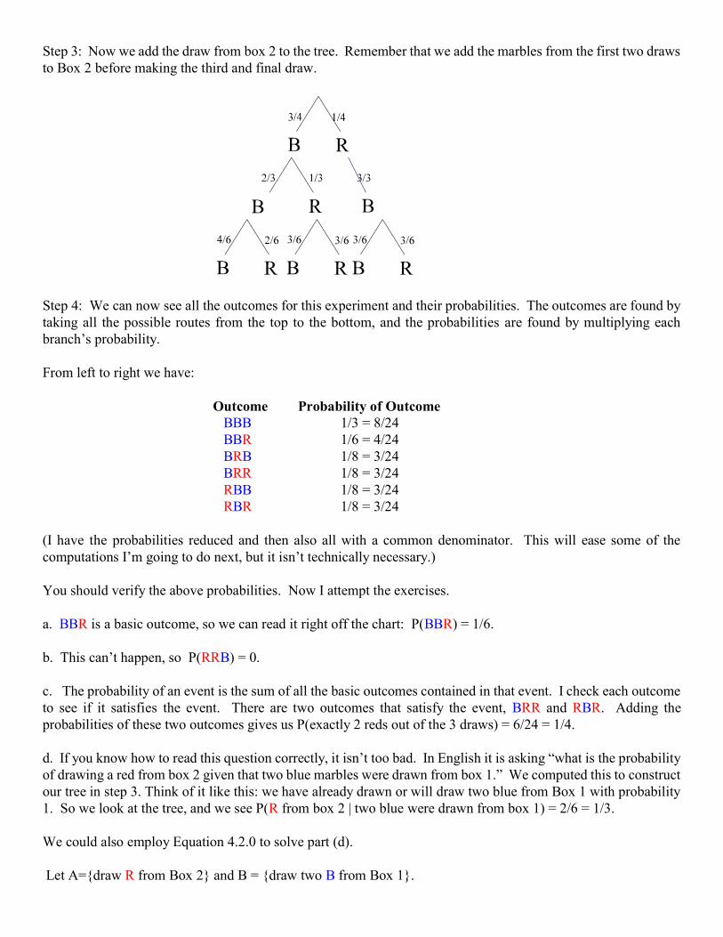
Step 3: Now we add the draw from box 2 to the tree. Remember that we add the marbles from the first two draws

to Box 2 before making the third and final draw.

Step 4: We can now see all the outcomes for this experiment and their probabilities. The outcomes are found by

taking all the possible routes from the top to the bottom, and the probabilities are found by multiplying each

branch’s probability.

From left to right we have:

Outcome Probability of Outcome

BBB 1/3 = 8/24

BBR 1/6 = 4/24

BRB 1/8 = 3/24

BRR 1/8 = 3/24

RBB 1/8 = 3/24

RBR 1/8 = 3/24

(I have the probabilities reduced and then also all with a common denominator. This will ease some of the

computations I’m going to do next, but it isn’t technically necessary.)

You should verify the above probabilities. Now I attempt the exercises.

a. BBR is a basic outcome, so we can read it right off the chart: P(BBR) = 1/6.

b. This can’t happen, so P(RRB) = 0.

c. The probability of an event is the sum of all the basic outcomes contained in that event. I check each outcome

to see if it satisfies the event. There are two outcomes that satisfy the event, BRR and RBR. Adding the

probabilities of these two outcomes gives us P(exactly 2 reds out of the 3 draws) = 6/24 = 1/4.

d. If you know how to read this question correctly, it isn’t too bad. In English it is asking “what is the probability

of drawing a red from box 2 given that two blue marbles were drawn from box 1.” We computed this to construct

our tree in step 3. Think of it like this: we have already drawn or will draw two blue from Box 1 with probability

1. So we look at the tree, and we see P(R from box 2 | two blue were drawn from box 1) = 2/6 = 1/3.

We could also employ Equation 4.2.0 to solve part (d).

Let A={draw R from Box 2} and B = {draw two B from Box 1}.

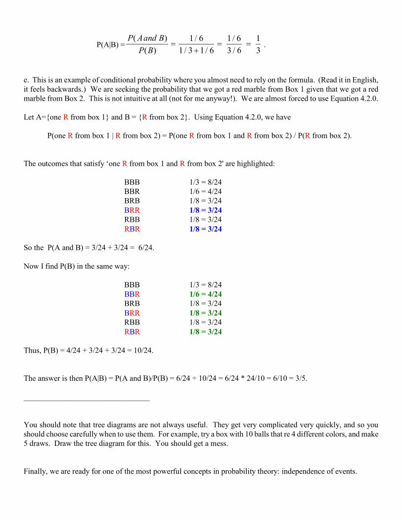
P(A|B) = .

e. This is an example of conditional probability where you almost need to rely on the formula. (Read it in English,

it feels backwards.) We are seeking the probability that we got a red marble from Box 1 given that we got a red

marble from Box 2. This is not intuitive at all (not for me anyway!). We are almost forced to use Equation 4.2.0.

Let A={one R from box 1} and B = {R from box 2}. Using Equation 4.2.0, we have

P(one R from box 1 | R from box 2) = P(one R from box 1 and R from box 2) / P(R from box 2).

The outcomes that satisfy ‘one R from box 1 and R from box 2' are highlighted:

BBB 1/3 = 8/24

BBR 1/6 = 4/24

BRB 1/8 = 3/24

BRR 1/8 = 3/24

RBB 1/8 = 3/24

RBR 1/8 = 3/24

So the P(A and B) = 3/24 + 3/24 = 6/24.

Now I find P(B) in the same way:

BBB 1/3 = 8/24

BBR 1/6 = 4/24

BRB 1/8 = 3/24

BRR 1/8 = 3/24

RBB 1/8 = 3/24

RBR 1/8 = 3/24

Thus, P(B) = 4/24 + 3/24 + 3/24 = 10/24.

The answer is then P(A|B) = P(A and B)/P(B) = 6/24 ÷ 10/24 = 6/24 * 24/10 = 6/10 = 3/5.

________________________________

You should note that tree diagrams are not always useful. They get very complicated very quickly, and so you

should choose carefully when to use them. For example, try a box with 10 balls that re 4 different colors, and make

5 draws. Draw the tree diagram for this. You should get a mess.

Finally, we are ready for one of the most powerful concepts in probability theory: independence of events.

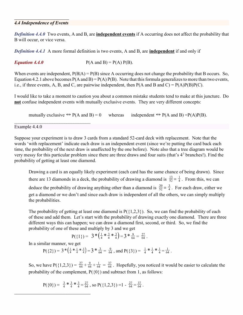
_______________________4.4 Independence of Events

Definition 4.4.0 Two events, A and B, are independent events if A occurring does not affect the probability that

B will occur, or vice versa.

Definition 4.4.1 A more formal definition is two events, A and B, are independent if and only if

Equation 4.4.0 P(A and B) = P(A) P(B).

When events are independent, P(B|A) = P(B) since A occurring does not change the probability that B occurs. So,

Equation 4.2.1 above becomes P(A and B) = P(A) P(B). Note that this formula generalizes to more than two events,

i.e., if three events, A, B, and C, are pairwise independent, then P(A and B and C) = P(A)P(B)P(C).

I would like to take a moment to caution you about a common mistake students tend to make at this juncture. Do

not confuse independent events with mutually exclusive events. They are very different concepts:

mutually exclusive � P(A and B) = 0 whereas independent � P(A and B) =P(A)P(B).

________________________________

Example 4.4.0

Suppose your experiment is to draw 3 cards from a standard 52-card deck with replacement. Note that the

words ‘with replacement’ indicate each draw is an independent event (since we’re putting the card back each

time, the probability of the next draw is unaffected by the one before). Note also that a tree diagram would be

very messy for this particular problem since there are three draws and four suits (that’s 43 branches!). Find the

probability of getting at least one diamond.

Drawing a card is an equally likely experiment (each card has the same chance of being drawn). Since

there are 13 diamonds in a deck, the probability of drawing a diamond is . From this, we can

deduce the probability of drawing anything other than a diamond is . For each draw, either we

get a diamond or we don’t and since each draw is independent of all the others, we can simply multiply

the probabilities.

The probability of getting at least one diamond is P({1,2,3}). So, we can find the probability of each

of these and add them. Let’s start with the probability of drawing exactly one diamond. There are three

different ways this can happen; we can draw a diamond first, second, or third. So, we find the

probability of one of these and multiply by 3 and we get

P({1}) = = = .

In a similar manner, we get

P({2}) = = = , and P({3}) = = .

So, we have P({1,2,3}) = + + = . Hopefully, you noticed it would be easier to calculate the

probability of the complement, P({0}) and subtract from 1, as follows:

P({0}) = = , so P({1,2,3}) =1 - = .

________________________________