Chapter 4 Manufacturing Process Control and Systems Control

4.1 Introduction(1) In this chapter, we will discuss manufacturing process control and manufacturing systems

control methods.

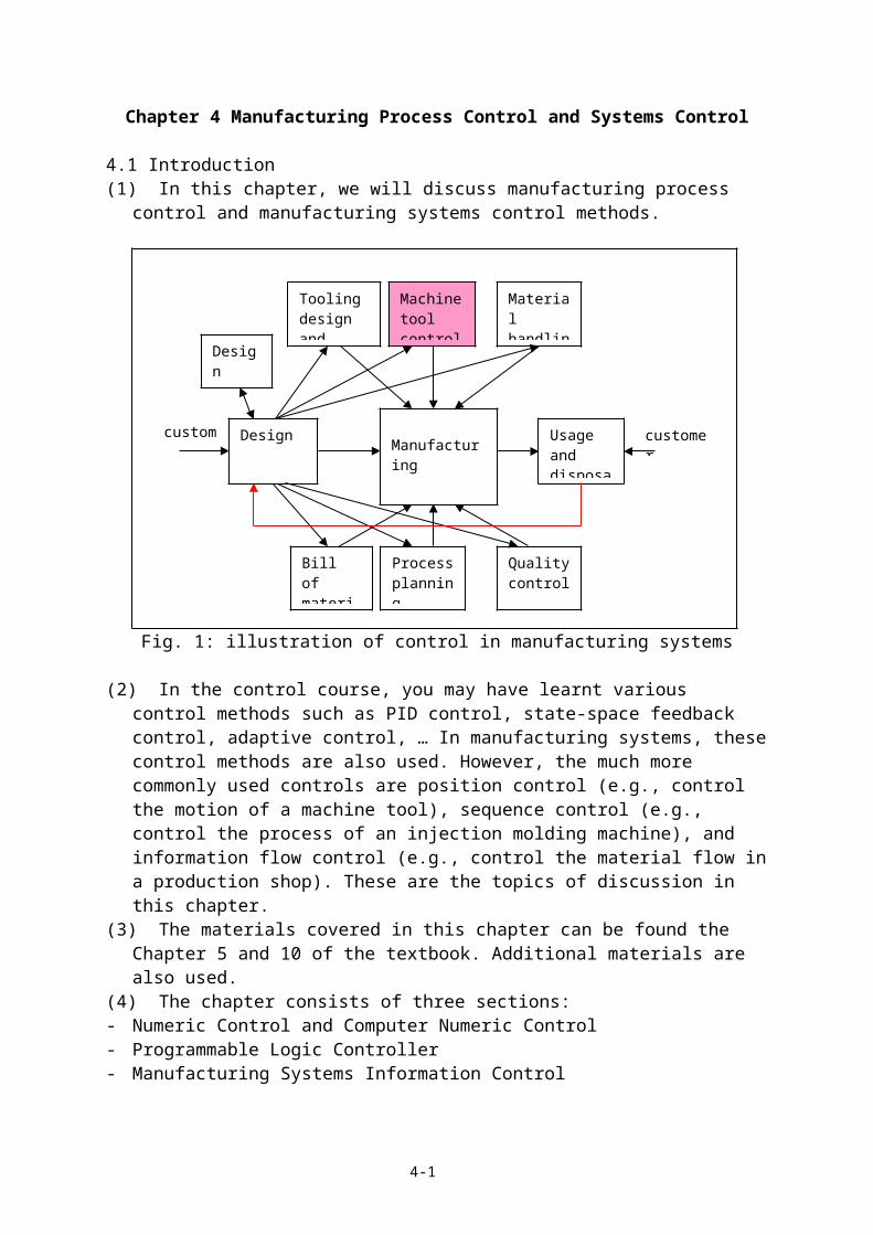
Fig. 1: illustration of control in manufacturing systems

(2) In the control course, you may have learnt various control methods such as PID control, state-space feedback control, adaptive control, … In manufacturing systems, these control methods are also used. However, the much more commonly used controls are position control (e.g., control the motion of a machine tool), sequence control (e.g., control the process of an injection molding machine), and information flow control (e.g., control the material flow in a production shop). These are the topics of discussion in this chapter.

(3) The materials covered in this chapter can be found the Chapter 5 and 10 of the textbook. Additional materials are also used.

(4) The chapter consists of three sections:- Numeric Control and Computer Numeric Control- Programmable Logic Controller- Manufacturing Systems Information Control

4.2 Numeric Control (NC) and Computer Numeric Control (CNC)(1) A brief history of NC- the objective of the NC and CNC: control the position of a mechanical device such as the

table of a machine tool- it was first developed in MIT for the Department of Defense (US)- the first generation of NC:

- program language: M code and G code- computer interface: tape puncher and tape reader- controller: special designed system

- the second generation of NC (CNC)

4-1

customer customer

Design analysis

Process planning

Bill of materials

Material handling

Tooling design and analysis

Machine tool control

Quality control

Manufacturing Usage and disposal

Design

- program language: M code and G code, Automatic Programming Tools (APT)- computer interface: keyboard and monitor- controller: special designed “closed” system

- the third generation of CNC- program language: Computer Aided Manufacturing (CAM) packages- computer interface: network- controller: PC based open architecture controller

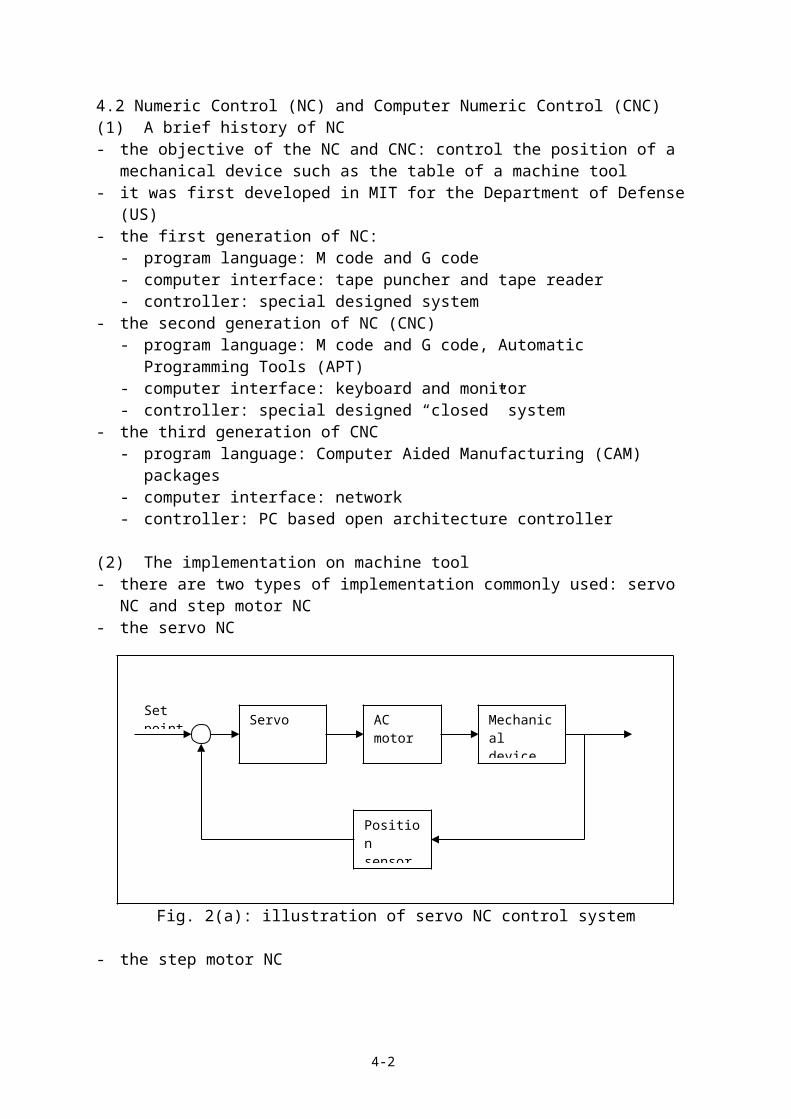
(2) The implementation on machine tool- there are two types of implementation commonly used: servo NC and step motor NC- the servo NC

Fig. 2(a): illustration of servo NC control system

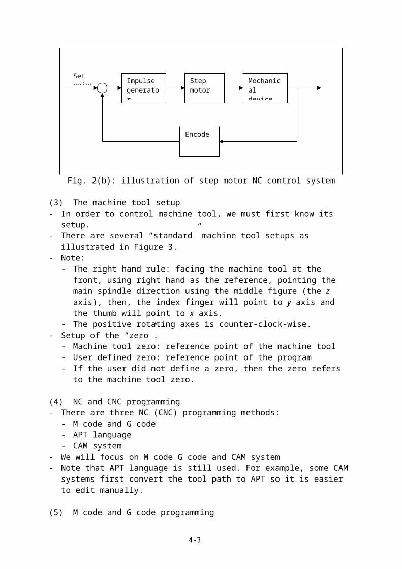
- the step motor NC

Fig. 2(b): illustration of step motor NC control system

(3) The machine tool setup- In order to control machine tool, we must first know its setup.- There are several “standard” machine tool setups as illustrated in Figure 3.- Note:

4-2

Servo AC motor Mechanical device

Position sensor

Set point

Impulse generator

Step motor

Mechanical device

Encode

Set point

- The right hand rule: facing the machine tool at the front, using right hand as the reference, pointing the main spindle direction using the middle figure (the z axis), then, the index finger will point to y axis and the thumb will point to x axis.

- The positive rotating axes is counter-clock-wise.- Setup of the “zero”.

- Machine tool zero: reference point of the machine tool- User defined zero: reference point of the program- If the user did not define a zero, then the zero refers to the machine tool zero.

(4) NC and CNC programming- There are three NC (CNC) programming methods:

- M code and G code- APT language- CAM system

- We will focus on M code G code and CAM system- Note that APT language is still used. For example, some CAM systems first convert the

tool path to APT so it is easier to edit manually.

(5) M code and G code programming- You may have learnt it in engineering practice- It is the “assembly language” of the CNC controller- the composition of a M code and G code command:

N0010 G00 X1.00 Z1.00 F0.1 S600where, N0010 is the block number, which is used to trace the program

G00 means incremental moveX1.00 is a geometric code meaning move to X = 1Z1.00 is a geometric code meaning move to Z = 1F0.1 means feed at 0.1 (its unit takes a default value)S600 mean spindle speed at 600 RMP

- Suppose the current tool position is (X, Z) = (0, 0) in a lathe, then the above command moves the tool to (X, Z) = (1, 1) in diagonal, i.e., the two axes move simultaneously with a spindle speed 600 RPM and feed rate 0.1 mm / rev.

- A list of M code and G code key words as shown below.

Table 4.1 Key words used in M code and G code programmingKey word Meaning

ABCFGIJKMNRSTU

Rotation about the x-axisRotation about the y-axisRotation about the z-axisFeed rate commandPreparatory function (refer to Table 4.2)Circular interpolation: x-axis offsetCircular interpolation: y-axis offsetCircular interpolation: z-axis offsetMiscellaneous commands (refer to Table 4.3)Block number of sequence number of the programRadius of arc or circleSpindle speedTool numberSupplemental coordinate parallel to x-axis

4-3

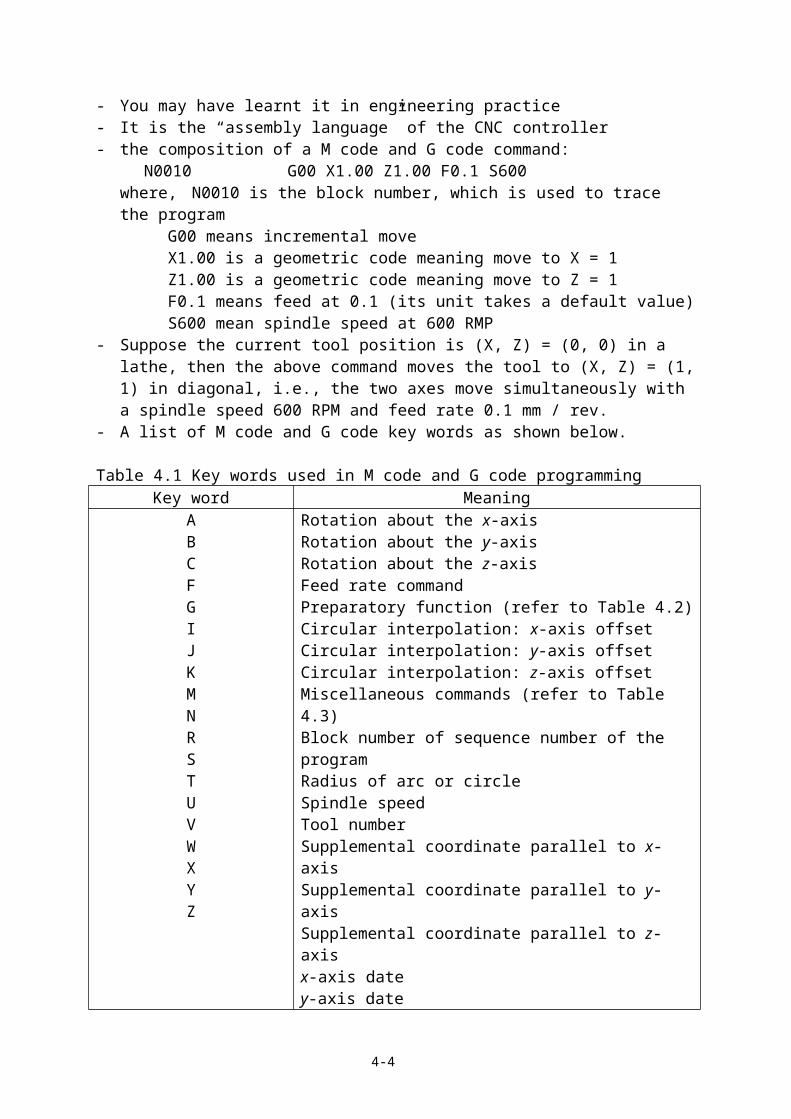
VWXYZ

Supplemental coordinate parallel to y-axisSupplemental coordinate parallel to z-axisx-axis datey-axis datez-axis date

Note: additional nonstandard keywords may also be used by individual manufacturers.

Table 4.2 Preparatory functionCode UsageG00G01G02G03G04G05G06G08G09G10G11G12

G13 – G16G17G18G19G20G21G30G31G33G34G35G40G41G42G43G44G53G54G55G56G57G58G59G62G63G64G70G71G80

Point-to-point positionLinear interpolationCircular interpolation (clockwise)Circular interpolation (counter-clockwise)Dwell for programmed durationDelay or hold (until resumed by operator)Parabolic interpolationControlled acceleration of feed rate to programmed valueControlled deceleration of feed rate to programmed valueLinear interpolation (long dimensions)Linear interpolation (short dimensions)Three-dimension interpolationAxis selection for machines with multiple headsx-y plane selectionz-y plane selectiony-z plane selectioncircular interpolation (clockwise, long dimensions)circular interpolation (clockwise, short dimensions)circular interpolation (counterclockwise, long dimensions)circular interpolation (counterclockwise, short dimensions)thread cutting, constant leadthread cutting, increasing leadthread cutting, decreasing leadcancel cutter compensation (see G41 and G42)cutter compensation, left (cutter to the left of the workpiece)cutter compensation, right (cutter to the right of the workpiece)cutter compensation, positive (re: radius of single-point lathe tool)cutter compensation, negative (re: radius of single-point lathe tool)cancel linear shift values (see G54-G59)linear shift, xlinear shift, ylinear shift, zlinear shift, xylinear shift, xzlinear shift, yzFast positioning (rarely used since advent of CNC)Tapping (rarely used since advent of CNC)Change feed rate (not required with CNC)Input dimension in inchesInput dimension in metric unitsCancel canned cycle (see G81-G89)

4-4

G81G82G83G84G85G86G87G88G89G90G91G92G94G95G96G97

Canned cycle for drillingCanned cycle for spot facing / counterboreCanned cycle for deep hole drillingCanned cycle for tappingCanned cycle for through boring (in and out)Canned cycle for through boring (in only)Canned cycle for chip breaker drillingCanned cycle for chip breaker drilling (with dwell)Canned cycle for through boring (with dwell)Input in absolute dimensionsInput in incremental dimensionsPreset in absolute registersFeed rate specified in millimeters (or inches) per minuteFeed rate specified in millimeters (or inches) per revolutionConstant cutting speed specified in millimeters (or inches) per minSpindle speed in revolutions per minute

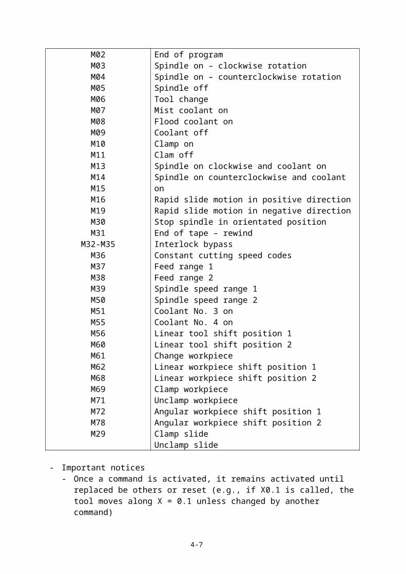
Table 4.3 Miscellaneous functionsCode UsageM00M01M02M03M04M05M06M07M08M09M10M11M13M14M15M16M19M30M31

M32-M35M36M37M38M39M50M51M55M56M60M61M62

Program stopOptional program stopEnd of programSpindle on – clockwise rotationSpindle on – counterclockwise rotationSpindle offTool changeMist coolant onFlood coolant onCoolant offClamp onClam offSpindle on clockwise and coolant onSpindle on counterclockwise and coolant onRapid slide motion in positive directionRapid slide motion in negative directionStop spindle in orientated positionEnd of tape – rewindInterlock bypassConstant cutting speed codesFeed range 1Feed range 2Spindle speed range 1Spindle speed range 2Coolant No. 3 onCoolant No. 4 onLinear tool shift position 1Linear tool shift position 2Change workpieceLinear workpiece shift position 1Linear workpiece shift position 2

4-5

M68M69M71M72M78M29

Clamp workpieceUnclamp workpieceAngular workpiece shift position 1Angular workpiece shift position 2Clamp slideUnclamp slide

- Important notices- Once a command is activated, it remains activated until replaced be others or reset

(e.g., if X0.1 is called, the tool moves along X = 0.1 unless changed by another command)

- The canned cycles can cut down the programming time- Additional preparatory functions have been developed recently (e.g., polynomial

interpolation)- To be able to program a CNC machine tool requires a lot of practice

(6) Examples- Example 1: a turning example – write a NC program to machine the simple aluminum pin

shown in Figure 4, assuming that- The center of the left face of the pin is set as the program zero- The tool start position is 0.2 in. off the diameter and 0.1 in. off the right face- Two roughing cuts (0.1 in deep) and one finish cut (0.05 in deep) will be taken,- A spindle speed of 12 rpm and feed rated of 1200 and feed rate of 12 inch / min are

used for machining- X values are to be programmed as diameters

Fig. 4: illustration of the turning example

- the program and interpolation% Indicates the start of the programN005 G90 G70 Specifies absolute programming, inch unitN010 G98 G92 T01 Specifies units for speed and feed rate, loads 1st

toolN015 G00 X1100 Z2700 F0 Rapid positioning of tool to tool start positionN020 X900 M03 S1200 F0 Position tool to remove 0.1 in. off part diameter,

start spindleN025 G01 Z500 F12 Feed tool into workpieceN030 X1000 Retract tool (overlap pervious cut)N035 G00 Z2700 F0 Move tool clear of workpiece

4-6

1.5

Tool start position

2.0

Material removed in one pass

2.52.0

Zero datum

0.1

0.2

N040 X800 F0 Position tool to remove 0.1 in. off part diameterN045 G01 Z500 F12 Feed tool into workpieceN050 X900 Retract tool (overlap pervious cut)N055 G00 Z2700 F0 Move tool clear of workpieceN060 X750 F0 Position tool to take finish cutN065 G01 Z500 F12 Feed tool into workpieceN070 X1000 Retract tool clear of the workpieceN075 G00 X5000 Z5000 F0 Move to safe positionN080 M30 Turn off all machine functions

- Example 2: a milling example: mill the exterior of the part shown below:

Fig. 5: illustration of the milling example

- Assume that- The size of the cutter is 10 mm- The part is on the z = 0 plane and the depth of cut is 10 mm. - The part has been pre-shaped and hence, it is not necessary to ramp

- Note that there are several critical points that must be determined first- The center most cutter location (-0.1346, 0), (refer to the small diagram for the

geometry calculation)- The left (right) most cutter location (-250.5, -100)- The left (right) most and bottom most cutter location (-250.5, -100.5)

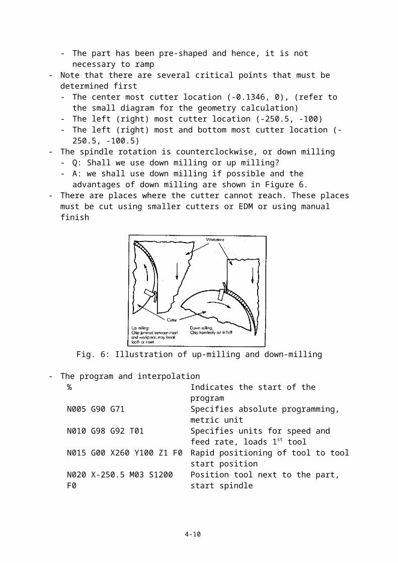
- The spindle rotation is counterclockwise, or down milling- Q: Shall we use down milling or up milling?- A: we shall use down milling if possible and the advantages of down milling are

shown in Figure 6.- There are places where the cutter cannot reach. These places must be cut using smaller

cutters or EDM or using manual finish

4-7

500

200(0, 0)

(-1.346, 0)

(-250.5, -100)

(-250.5, -100.5)

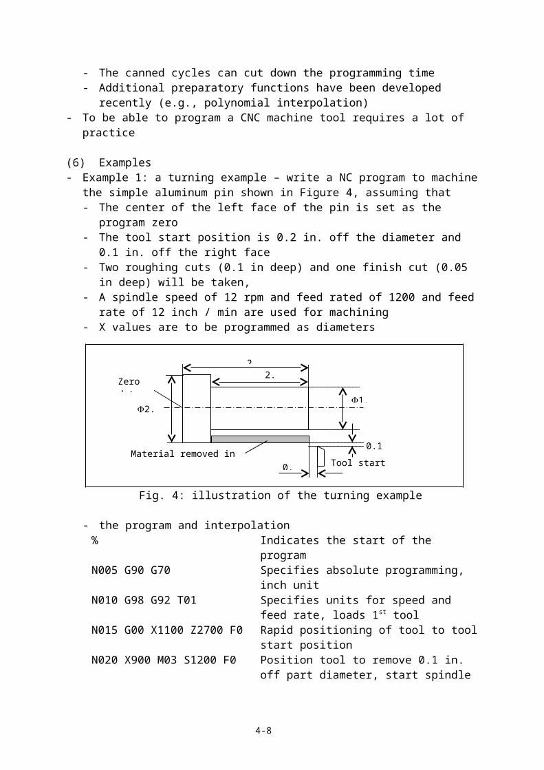
Fig. 6: Illustration of up-milling and down-milling

- The program and interpolation% Indicates the start of the programN005 G90 G71 Specifies absolute programming, metric unitN010 G98 G92 T01 Specifies units for speed and feed rate, loads 1st

toolN015 G00 X260 Y100 Z1 F0 Rapid positioning of tool to tool start positionN020 X-250.5 M03 S1200 F0 Position tool next to the part, start spindleN025 G01 X-1.346 Y0 F3000 Feed tool into workpieceN030 X-250.5 Y-100 Continue to cutN035 Y-100.5N040 X250.5 Clear the bottom…… ……

- There are several additional examples in the textbook

(7) CAM system programming- The need of CAM programming: even using an advanced programming language (e.g.,

APT), CNC programming is tedious and complicated. Sometimes it is nearly impossible (e.g., machining a complex mold or die). Hence, people invent the copy machine, which copies the geometry from a real size wood model. More recently, Computer Aided Manufacturing (CAM) systems become the mainstream.

- Many CAM systems have been developed. I know about 20 such as: CATIA (France), Powercut (England), UniGraphics (USA), I-DEAS (USA), Gibbs (USA), Cimetron (Israel) …

- The procedure of CAM programmingStep 1: job setupStep 2: tool design (generate machine-able volume)Step 3: generate rough machining tool pathStep 4: generate finish machining tool pathStep 5: run a computer simulation and testStep 6: download the tool path to the machine tool

We will discuss these steps in more details below.

(8) Job setup in a CAM system- While CAM systems may be different, they all require a procedure to setup the job first

4-8

- The job setup shall include- Read in the design of the part (a mold, a die, or a tool)- File conversion - some CAM systems use their own special internal data format and

hence they will convert a design file (mostly in IGES format or STEP format) to its own format first

- Read in the stock- Read in the machine tool setup (the coordinate system and zero datum)

- Job setup is the most confusing step to the beginners. As they first get in a CAM system, there are many icons, commands, and etc. laid in front. It is rather difficult to figure out where to start.

(9) Tool design (generate machine-able volume)- Many (if not all) CAM systems have built-in functions for computer aided design- The basic operation of the tool design is to generate machine-able volume by impinging

the part on the stock as shown Fig. 7.- Note that the molds and dies always come in pair. In addition, there may be several

inserts

Fig. 7: Illustration of tool design based on the part

- It should be noted that the design of the mold or die is much more than impinging the part on the stock. It also involves the design of raisings, run ways, cooling lines, mounting holes, etc.

(10) Generate rough machining tool path- In roughing, the objective is to remove as much material as possible in a short time. - Roughing is usually done using flat end mills cutting one layer at a time. Hence, it is

sometime referred to as step machining.- The first step of roughing tool path generation is to decide on manufacturing strategies. In

the previous chapter, we have studied the machining process somewhat in details and knew how to calculate the optimal cutting speed, tool life and machining time. The same principles are applied here as well.

- The additional problems encountered here include:

4-9

Stock tool

Part

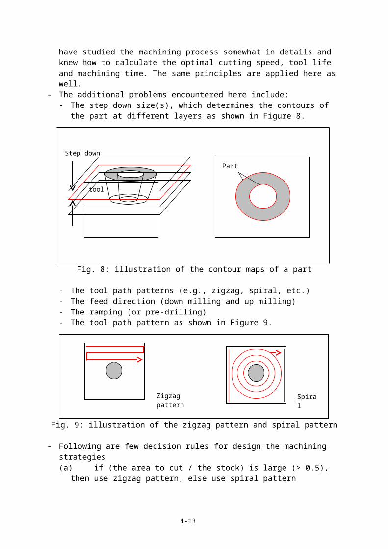
- The step down size(s), which determines the contours of the part at different layers as shown in Figure 8.

Fig. 8: illustration of the contour maps of a part

- The tool path patterns (e.g., zigzag, spiral, etc.)- The feed direction (down milling and up milling)- The ramping (or pre-drilling)- The tool path pattern as shown in Figure 9.

Fig. 9: illustration of the zigzag pattern and spiral pattern

- Following are few decision rules for design the machining strategies(a) if (the area to cut / the stock) is large (> 0.5), then use zigzag pattern, else use spiral

pattern(b) if there are multiple islands / cavities, decompose the cutting areas into several zones

and machining them one at a time(c) ……

- The key to the roughing tool path is contour offset- Given a plane curve, {x(t), y(t)}, its offset curve can be represented as follows:

where, d is the offset distance.

4-10

Zigzag pattern

Spiral pattern

tool

Step down size

Part contour

- An example: give a line segment:x(t) = x1 + t(x0 – x1)y(t) = y1 + t(y0 – y1)

the derivatives are:

the offset line segment is:

- Offset calculation is in fact rather complicated as shown in the previous example. The following figure shows another example

Fig. 10: illustration of the contour offset in roughing

(11) Generate finish machining tool path- Rough machining lefts a number of steps on the part. The objective of finish machining is

to remove these steps and to get the final shape as close as possible- There are two types of finish machining methods: 3 axes machining using ball end mills

or 5 axes machining using Taurus mills. The former is the most commonly used methods while the later is more efficient, though more complicated.

- Finish machining tool path is also based on offset: surface offset- For complicated surfaces, the surface offset calculation is very complicated. Hence, most

CAM systems use surface data maps and calculate the surface offset based on triangulation. The details of this method are beyond the scope of this class.

(12) Run a computer simulation and test- In order to ensure that the tool path runs correctly, it is necessary to conduct a computer

simulation so that the user can examine the tool path section by section.

4-11

Part contour

Loops in the tool path

- Most CAM systems have build in computer simulation functions.- Advanced computer simulation can also identify the materials left and generate another

tool path to clear them. This greatly helps to improve the accuracy of machining and to minimize the subsequent manual polishing operations

(13) Download the tool path to the machine tool- After the tool path is verified, it can be directly download to the machine tool. This is

done through the standard computer I/O ports such as RS232 series port. New machine tools have parallel ports as well.

- The current trend is to have a cutter path generation on the shop floor next to the machine tool. In other words, there are two computers working side by side. One is used to control the machine tool. The other is used by the operator to generate and examine the tool path for the subsequent cuts.

(14) A special lab is organized to show a CAM system, Gibbs.

4.3 Programmable Logic Controller (PLC)(1) Today, most machines and manufacturing processes are still controlled not by PC

(personal computer but by PLC (programmable logic controller). This is mainly due to two reasons. First, the required control functions are relatively simple (e.g., on-off control, sequence control, etc.). Second, the controller must be very reliable under various situations.

(2) PLC was first developed in 1960s to handle logic (on / off) and sequential controls. Today, the major manufacturers of PLC include Texas Instrument, Allen-Bradley and Toshiba. PLC has several advantages including:

- easy to program- able to handle a large number of I/Os with high and low voltages- very reliable(3) Examples of PLC applications- lifts in buildings- traffic lights- injection molding machines- electric power generation stations

4-12

Memory I/O

Power supply

CPU

Fig. 11: the construction of a PLC

- ……(4) As shown in Figure 11, PLC consists of four parts: (a) CPU, (b) memory, (c) power

supply and (d) I/O.- Most PLCs use special CPUs rather than Intel Pentium- Most PLCs have an EPROM (memory) for customer programs- PLCs must have a power supply - PLCs can handle a large number of I/Os (say a couple of thousand).- The accessories of PLC include: Keyboard or teach pendant and Monitor(5) How to program a PLC.- As pointed out early, PLC is used to deal with logic and sequential control. So, the key to

program a PLC is to develop the logic- There are a number of ways to represent a logic operation. The following examples

shown three different methods by means of a simple example.- An simple example: machine control by authorized person only

Fig. 12: an simple control example: machine access by authorized person only

- In this example, it is required that the machine being controlled (turn-on or turn-off) by authorized person (have a key) only.

- Define:- K = 0 (no key is presented) and K = 1 (key is presented)- S = 0 (switch to off position) and S = 1 (switch to on position)- M = 0 (the machine is not running) and M = 1 (the machine is running)- MC = 0 (the machine is stopped) and MC = 1 (the machining is started)

- The control logic can be represented by the truth table:

K S M MC0 0 0 00 0 1 10 1 0 00 1 1 11 0 0 01 0 1 01 1 0 11 1 1 1

- The truth table is simple and straightforward. However, it is tedious and difficult to use in dealing with complicated problems.

4-13

M machinekey

switch

K

S

- The second method is to use Boolean operators. For the above example, it can be shown that the problem can be represented by the Boolean operator below:

which can be verified case by case.- However, the Boolean operators are usually difficult to find. In fact, for complicated

problems with dozens of variables, it is very difficult to find the right Boolean operator.- The third and the most effective method is the ladder diagram.

(6) Ladder diagram- The ladder diagram constructs the logic step by step.- A ladder diagram consists of just a few basic elements:

- The left rail represents the power line- The right rail represents the ground

- Between the two rails, there may be as many rugs as possible and each rug represents an independent logic operation such as “and” (represented by series connection) or “or” (represented by parallel connection) or “not” (represented by a cross bar).

- Each rug may have many contacts, representing the logic conditions, but must have a load, representing the power sink (otherwise, there will be short circuit).

- The load of a rug can be the contacts of other rugs and itself.- All the rugs are executed simultaneously.

- Figure 13 shows the ladder diagram of the console lock example above- Enter the ladder diagram to PLC

- Modern PLCs have graphic user interface- We can use the PLC language as well. For the above example, a sample PLC program

is:MC = (K.and.S).or.(not.K.and.M)

- Each PLC manufacturer may have its own format but they are all similar.- Today, graphic driven programming tools are also available.

(7) The other important components in PLC: contact, counter and timer- PLC may be connected to contacts or relays. In this case, their logic must be considered

as well.- As shown in Figure 14, there are several types of contacts including:

- Normal on- Normal off- Push on- Push off

4-14

K S

K M

MC

Fig. 13: the ladder diagram

- Rotary contactsIt should be noted that Normal on is the opposite of Normal off, Push on is the opposite of Push off.

- It is interesting to know that PLC was first developed to replace the contacts.- Counter is very important. There are several types of counters

- Counter up (CTU)- Counter down (CTD)- Counter reset (CTR)

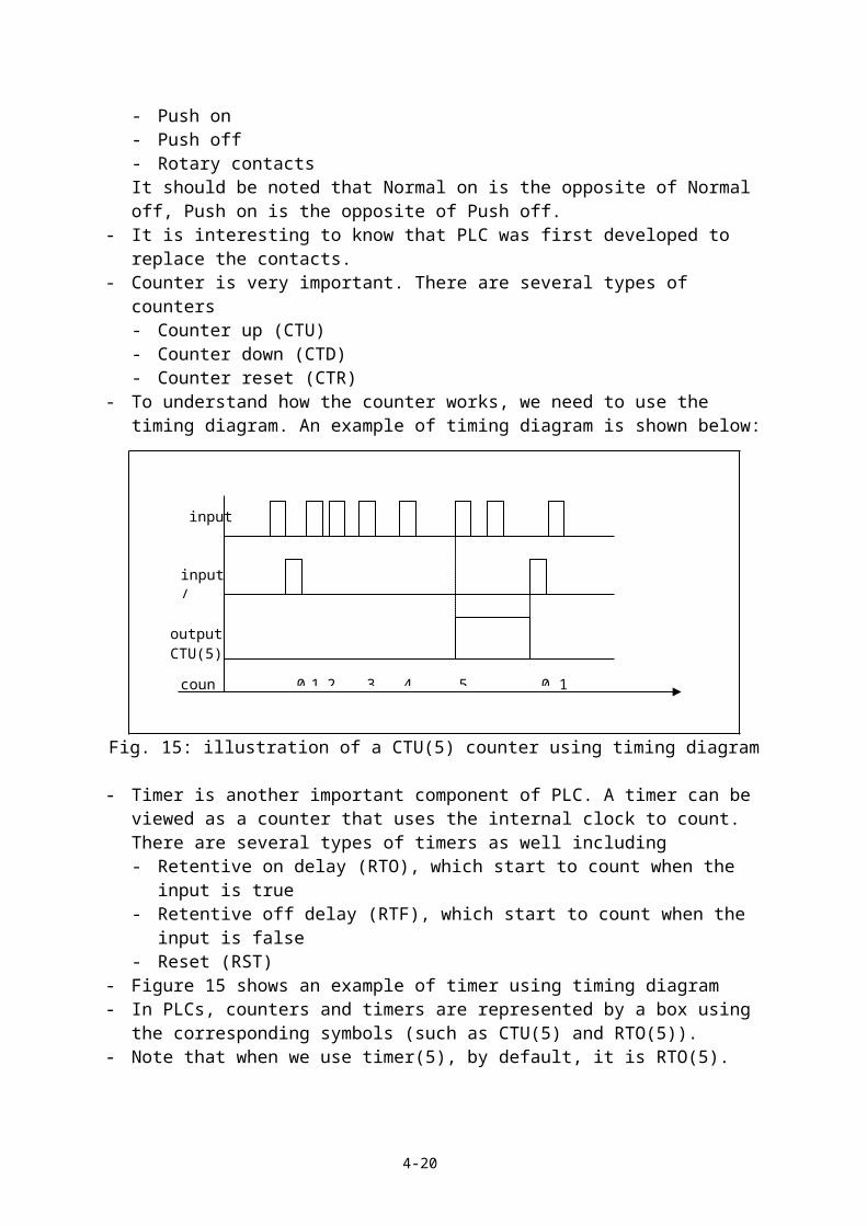
- To understand how the counter works, we need to use the timing diagram. An example of timing diagram is shown below:

Fig. 15: illustration of a CTU(5) counter using timing diagram

- Timer is another important component of PLC. A timer can be viewed as a counter that uses the internal clock to count. There are several types of timers as well including- Retentive on delay (RTO), which start to count when the input is true- Retentive off delay (RTF), which start to count when the input is false- Reset (RST)

- Figure 15 shows an example of timer using timing diagram- In PLCs, counters and timers are represented by a box using the corresponding symbols

(such as CTU(5) and RTO(5)). - Note that when we use timer(5), by default, it is RTO(5).

4-15

input

input / reset

outputCTU(5)

count 0 21 3 4 5 0 1

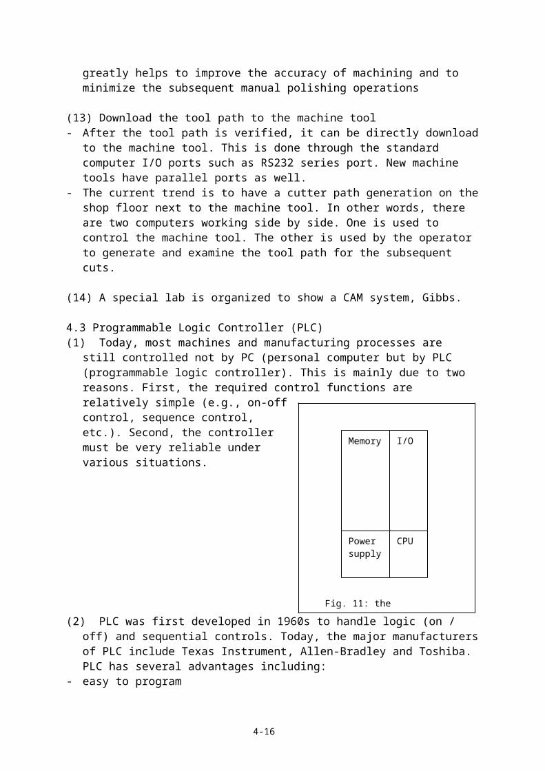
Fig. 15: illustration of a timer using timing diagram

(8) PLC programming- PLC programming consists of four steps:

Step 1: setup the I/OsStep 2: develop the ladder diagramStep 3: test the ladder diagram (computer simulation)Step 4: download

- The best way to show how to program PLC is by means of examples. We had a very simple example above and we will give two additional examples below.

(9) Example 1: machine loading and unloading to AGV (Automatic Guided Vehicle)- This example is in the textbook (example 6.6)- Actions required:

- Sensor 1 signals the arrival of the AGV- Sensor 2 signals AGV bring in raw parts - Sensor 3 signals AGV has room available to carry completed parts- Sensor 4 signals the machine being loaded or signals the completion of processing a

part - Robot unloads a completed part from machine to AGV- Robot loads a new part from AGV to machine- AGV dispatches

- PLC programming Step 1: defining the I/OI/O Meaning / Associated actions01020304202122

AGV has arrivedAGV is carrying a new part to be processedAGV has space to store a processed partMachine has a finished part to be unloadUnload completed part from machine onto AGVPick a new part from the AGV and load onto the machineDispatch the AGV

- PLC programming Step 2: develop the ladder diagram- There are three loads (20, 21, 22) and hence, we need at least three rungs

4-16

clock

input / reset

output RTO(5)

count 0 21 3 4 5 0

- The first rung represents the logic of unloading a completed part from machine onto AGV, and its condition is AGV has arrived (01) and AGV has space to store a processed part (03) and machine has a finished part to be unload (04)

- The second rung represents the logic of picking a new part from the AGV and loading onto the machine, and its condition is that the part has been unloaded from (20) or AGV has arrived (01) and machine does not have finished to unload (~ 04), and AGV is carrying a new part to be processed (02)

- The third rung represents the logic of dispatching the AGV. You are invited to figure out the logic.

In summary, the ladder diagram is shown below.

Fig. 16: the ladder diagram of the AGV example

- PLC programming Step 3: testing the ladder diagram. - PLC programming Step 4: downloading

(10) Example 2: traffic light control- Action required: control the traffic light following the timing (in sec.) below:

LightStreet Red Yellow Green TotalMain St. 30 10 40 80Jordan St. 50 10 20 80

Note that the row sum must be equal.- Definition of I/Os:

- There is no input (timing based on an internal clock)- Outputs:

64 – JR (Jordan red)65 – JY (Jordan yellow)

4-17

20

21

22

01 03 04

20

21

0401

01

20

02

02

04

01

02

20

04

03

21

22

66 – JG (Jordan green)74 – MR (Main red)75 – MY (Main yellow)76 – MG (Main green)

- the timing diagram

Fig. 17: the timing diagram of the traffic light example

- There are several ways to develop the control logic. In fact, for most applications, there is more than one solution. For the traffic light example, there are at least two ways to turn the JR on as shown below:- If neither JG nor JY is on, then JR is timed for 50 sec.- If either MR or MY is on, then JR is timed for 50 sec.

Fig. 18: Two different ladder diagrams for a same purpose

- In summary, the ladder diagram is shown in Figure 19.

4-18

JR

JY

JG

MR

MY

MG

0 80

Timer(50) 6

4

65

66

Timer(50) 6

4

74

75

(a) (b)

Fig. 19: The PLC diagram of the traffic light control example

- In practice, much more situations must be considered such as- Synchronization with the other traffic lights- Emergency situation (traffic accidents)- Power outrage- ……

(11) Group discussions and presentations.

4.4 Manufacturing Systems Information Control(1) In the previous sections, we have learnt how to control various machines including CNC

machine tools (position control) and transfer lines (sequence control). There are several special types of machines that have their own methods of control. For example, robot and AGV have their own control systems and programming language. From a manufacturing system point of view, however, we need another type of control. That is to control the production flow, the material flow, job flow, etc. We call such a system the manufacturing shop floor control system.

4-19

64

65

66

64

65

74

66

75

76

Timer(50)

65

66

Timer(10)

66

65

Timer(20)

74

76

Timer(30)

75

76

Timer(10)

76

75

Timer(40)

64

64

75

74

74

(2) In theory, the manufacturing operation shall follow the designed process plan (as we discussed in Chapter 3). In practice, however, many problems may occur, such as machine break down, material supply halt, worker absent. Therefore, it is necessary to continuously monitor the manufacturing operations. This is another reason to use the manufacturing shop floor control system.

(3) Figure 21 illustrates the manufacturing shop floor control system.

Fig. 21: Illustration of manufacturing shop floor control system

- The objective of the manufacturing shop floor control system is to collect information regarding to the operation (and take reactions accordingly). Note that human managers are needed to implement the control such as change the production schedule and order spare parts.

- The primarily hardware of a manufacturing shop control system include:- Main server and accessories (e.g., printer)- PC computers- Bar code readers

- As shown in the figure, a typical manufacturing shop floor control system will have a main server, which connects to several PCs. Each PC interface to a number of bar code readers that collect information on material flow, job flow and etc.

- The critical technology in manufacturing shop floor control systems include information collection devices (bar code reader and smart card) and computer networking (hardware, software and network protocol). Since the later has been discussed in other courses, in the remaining of this chapter, we will focus on bar code reader and smart card.

(4) The basics of bar code reader- Although simple, bar bode reader is a critical component that changes the face of modern

manufacturing.- The bar code itself consists of a sequence of thick and narrow dark bars separated by

thick and narrow spaces as shown below.

4-20

Main server printer

PC PC PC

Bar code reader

Bar code reader

Bar code reader

Bar code reader

Bar code reader

Bar code reader

Fig. 22:

Illustration of the working principle of a bar code reader

- The bar code reader consists of a scanner and a decoder. The scanner emits a beam of light that is swept past between the bars and spaces. The light reflections are sensed by a photodetector that converts the spaces into an electric signal (1) and the bars into absence of an electric signals (0).

- Bar codes can be attached onto the parts using various methods such as- Direct printing- Self stick label- Laser etching- …

- There are various codes. The most commonly used codes include:- Universal Product Code (UPC), adopted by the grocery industry.- Code 39 (or 3 of 9 code), adopted by the U. S. Dept. of DefenseThe other codes are briefly described in the textbook.

(5) Code 39- Code 39 is so named because the code consists of 9 elements (bars and spaces) are used

and 3 of which must be wide elements (bars and spaces). Similarly, Code 25 (2 of 5 Code) consists of 5 elements and 2 of which must be wide elements.

- It uses a uniquely defined series of wide and narrow elements to represent 0-9, the 26 alpha characters, and special symbols as shown in Figure 22. The wide element is equivalent to 1 and the narrow element is equivalent to 0.

- The width of the narrow bars and spaces, called the X dimension, provides the basis for a scheme of classifying bar codes into three code densities;- High density: X dimension is 0.010 inch or less- Medium density: X dimension is between 0.010 and 0.030 inch- Low density: X dimension is 0.030 inch or greaterWith X 0.02 inch, it is the wide element, else it is the narrow element. Whatever the wide-to-narrow ratio, the width must be uniform throughout the code.

- As an example, Figure 23 shows a bar and its interpretation. Note that the “quiet” zones in the beginning and the end of the code.

(6) The use of bar code in manufacturing shop floor control systems- With a properly setup of bar code system, one can easily trace the material flow and job

flow in the shop floor- Figure 24 shows an example of job order based on the bar code technologies- Other applications of bar code in factory automation include:

- Service and maintenance tracking

4-21

light

Reception signal

- Order and spare parts tracking- …

(7) Smart cards- The history of cards: cards have been used for centuries to retain / send simple messages.

However, in the past two decades, with the advance of computer technology, we have now the banking card, the telephone card, the security card, the credit card, … Arguably, we cannot even live without them.

- There are several types of smart cards commonly used today. These include:- Identification cards (it uses bar codes)- Magnetic strip cards- Optical cards- Chip cards

- These cards are very cost effective. Following table shows the costs of these cards in US dollars.

Card unit cost Attached reader Standalone readerMagnetic strip 0.15 – 0.6 15 – 20 (2 tracks)

25 – 50 (3 tracks)150 – 600 (with PC)300 – 1000 (POS)10,000 (ATM)

Optical 4 – 8 N / A 800 – 3000 (PC)Chip cards

Memory 0.5 – 5 100 – 200 (with PC)Smart card 3 – 15 300 – 900 (with PC)

Super smart 20 – 50Contact-less 5 - 20

- Let us first look at the magnetic strip cards. Figure 25 illustrates the working principle of a magnetic card.

Fig. 25: Illustration of the working principle of magnetic cards

- Magnetic cards are passive cards (the operations must be initiated and done by external devices) and their storage capacity is limited. In comparison, the chip cards (smart cards) provide more storage space and operations.

- Figure 26 shows an example of smart card, in which an miniature computer is build in the card. Consequently, it can handle much more information and operations.

4-22

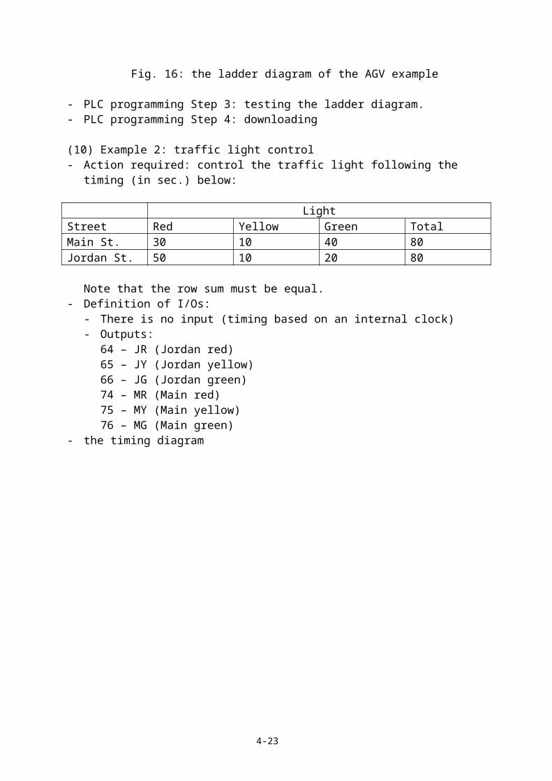
Fig. 26: Illustration of the working principle of a magnetic card.

(8) Concluding remarks- Currently most manufacturing shop floor control system are really supervision (instead of

control) system as it only collects information and the human managers have to react accordingly (e.g., change the production schedule, order additional material and etc.). More advanced manufacturing control systems are also used in practice, for which the students are referred to the references.

4-23