Chapter 4: Landslide model (SLIDE}

This chapter deals with the mathematical background, assumptions and programming

of the coupled hydrological-soil mechanical landslide prediction model script (called

SLIDE). By definition, physically based statistical and deterministic models (Section

1.3) such as the one described in this chapter, consist of various separate calculations

for the hillslope hydrology and slope stability components (Sidle et al., 1985).

Calculations are based on the models of Montgomery and Dietrich (1994), Borga et al.

(1998) and others (Chapter 3). Equation variables will be replaced by the field

measurements listed in Table 3.1.

Programming of the SLIDE script was done with PCRaster Geographic Information

System (GIS) (Utrecht University, 1994). Motivation for modelling in a GIS is twofold:

first, the drainage direction of water over undulating topography can be· simulated

spatially and second, landslides have spatial occurrence and predictions made by the

SLIDE model can easily be viewed and interpreted on a model output map.

4.1 Equations for the landslide prediction model (SLIDE)

The model used for landslide prediction in the Injisuthi Valley is composed of two

parts: a planar infinite-slope Coulomb failure model (Section 4.1.1) and a steady state

subsurface flow model (Section 4.1.2). Planar infinite slope analysis has previously

been applied in investigations of slope stability, particularly where the thickness of the

soil mantle is much lower than the length of the slope and where the failure plane is

approximately parallel to the slope surface (Terlien, 1996; Borga et al., 1998). In this

study the infinite slope model will be applied to the Injisuthi Valley where the

landscape is represented by maps with symmetrical pixels or grids containing values

as they were measured in the field (Chapter 3).

A hydrological model for steady state subsurface flow computes the depth of the flow

for each map grid in the basin. In the model, slope-parallel flow assumption is adopted

because it is designed for shallow translational failure. Deviations from slope-parallel

flow have been noted to occur, especially in deeper soils where the flow vector will

affect the calculations of shear strength (section 3.3.4.2) (Iverson and Major, 1986).

However, an order of magnitude difference in hydraulic conductivity between the soil

and subsurface stratum can cause groundwater to flow nearly parallel to the drainage

barrier (Reid and Iverson, 1992). While assuming parallel flow, SLIDE is underpinned

by the following assumptions:

1. The lateral subsurface flow rate is assumed to be proportional to the local slope of

the terrain. This implies kinematic flow and that the water table is parallel to the

topography (Borga et al., 1998).

2. Hydraulic conductivity varies between two soil layers (Chap~er 3; section 3.3). The

upper and lower layers are assumed to take up similar fractions with varying soil

depths throughout the study area S.

3. Recharge is assumed to be spatially uniform within the study site.

4. Steady-state conditions are assumed to apply so the subsurface flow rate is

proportional to the recharge and the specific up-slope area as defined by the local

drainage direction map.

5. Recharge rate is defined by Darcy's law of water flow.

6. Storage, inputs and outputs of water in each pixels are subject to the mass

conservation principle (Thomas and Huggett, 1980), therefore a general water

storage equation of the block may be written as: change of water in block is equal

to water inputs minus water outputs.

7. As the soil becomes saturated, the excess precipitation that cannot enter the soil

profile is lost in the form of saturation excess overland flow.

8. Hortonian overland flow occurs where rainfall intensity exceeds the infiltration

capacity of the topsoil layer.

9. As a rule, cohesive soils form a circular rather than planar slip surface (Veder,

1981). One exception to this rule, however, is where vertical stratification of the

cohesive soil layers are present, a planar slip surface is likely to form (Veder,

1981). In Chapter 3 (section 3.4) the vertical stratification of the soil is discussed

with regards to the orthic A and soft plintic B horizons and therefore model

calculations assume a planar slip surface, discussed in next section.

4. 1. 1 Infinite slope concept

After the parameters involved in slope instability have been identified, slope instability

must be quantified. Selby (1993) describes three basic failure model types that can be

used as the basis for landslide modelling. The first is the planar slip surface analysis

(infinite slope model). Second, the circular slip surface analysis, where a curved failure

plane is involved and the slope is divided into segments, and third, the noncircular slip

surface analyses, where the slip surface is divided into more segments in a irregular

slip surface (Selby, 1993). Of the three techniques the infinite slope analysis has the

broadest application for determining slope instability (Selby, 1993), and several

shallow landslide models for use at the basin scale have been developed on the basis

of the infinite slope equation (e.g. Montgomery and Dietrich, 1994; Wu and Sidle,

1995, Borga et al., 1998). According to Selby (1993) the infinite slope equation is also

the best for predicting surficial rainfall triggered landslides, as occur in the Injisuthi

Valley (Chapter 2).

The infinite slope concept was first described in 1776 by Coulomb who defined it as a

slope with a constant slope angle, infinite length and uniform condition at a certain

depth under the soil surface (Selby, 1993). Theoretically, a sliding plane of an infinite

slope runs parallel to the ground surface (Figure 4.1). Although the assumption for

uniformity is in reality never met, because the sliding plane will be slightly curved in

some instances, the infinite slope model forms a good basis for the analysis of slope

stability (Selby, 1993).

Upthrust= Yw' z...coS> a.

Normal stress(I" Ys.z.cos' a.

Forces acting on an element in a theoretically infinite slope (after Selby,

1993).

Forces acting at a point on a shear plane of a potential shallow slide are illustrated in

Figure 4.1. Selby (1993) describes the detailed derivation of equations and only the

most important steps will be highlighted here. The graVitational stress acts vertically

(overburden), the normal stress (an) is normal to the shear plane and it partly opposed

by the upthrust or buoyancy effect of pore-water pressure (Figure 4.1). The shear

stress ('t) acts down the shear plane and is restricted by the shear strength of the soil

(Figure 4.1). Effective shear strength ('tf) opposing the shear stress ('t) is given in the

Coulomb equation 4.1.

= effective cohesion (Pa=kN/cm2)

= normal stress imposed by the weight of solids and water (kN/cm2)

= pore water pressure derived from the unit weight of water (kN/cm2)

= effective angle shearing resistance (0)

The value of O"n is function of the weight imposed on a slope by water and soil and can

be determined indirectly through measurements of the vertical thickness of the soil

(Selby, 1993). The height to where the water table rises (zw) in a rainfall event may

reach a maximum height of the soil body (z). Changes in the water height cause

changes in the pore pressure and shear strength of the soil (equation 4.2).

= unit weight of soil (kN/cm3)

= unit weight of water (kN/cm3)

= z wlz (dimensionless)

= depth of failure surface below the surface (cm)

= height of water table above water surface (cm)

= angle of the topographical slope (0)

The factor of safety (F) (equation 4.3) can be calculated by dividing the shear strength

('tf) by the shear stress (were 't = Wsina, and hence 't = Ys zcosasina).

When shear strength and shear stress forces are in equilibrium, the slope is at the

point of failure and the safety factor (F) is equal to 1 (equation 4.3). When the shear

strength is smaller than the shear stress, the safety factor is smaller than 1 and the

slope will fail (in theory) (Selby, 1993). At the moment of failure, the shear stress

mobilises the shear strength of the slope (Selby, 1993), and F is therefore rather an

evaluation of the relationship between shear stress and mobilised shear strength.

Evident from equation 4.3 is that the height of the water table (z.,Jz) and SUbsequently

the pore water pressure are important components in slope stability analysis. In a

perfectly infinite slope with a uniform laminar flow in only one direction (downwards)

the equation (4.3) described above would be sufficient to construct a slope stability

model. In reality, however, the undulating topography of the Injisuthi valley results in

different drainage directions in the landscape and therefore different pore water

pressures exist at any specific point. Further, the amount of water that percolates to a

downstream pixel is dependent on the various soil moisture contents of the entire up

slope contributing area (or map pixels). For each specific pixel, two questions may be

asked. First, how much water will percolate into and out of a pixel at a specific time?

Second, in which direction does the water percolate? These questions will be

addressed in the next section on hydrological calculations.

4. 1.2 Hydrological calculations

Landslide locations in the Injisuthi Valley are directly related to the hydrological

changes in the soil (Chapter 2). Rainfall-induced landslides all over the world, for

example Italy (Borga et al., 1998) and Colombia (Van Westen and Terlien, 1996), are

caused ultimately by a relative increase in pore pressure of the soils, which often

develop over a contact between texturally different soil horisons (the case for the

Injisuthi Valley, Chapter 3) or between the soil and bedrock contact. Components of

the hydrological cycle that are relevant to shallow landslide modelling are summarised

in Figure 4.5 as a series of storages and flows. The sequence of numerical

calculations in SLIDE follow the sequence starting with atmospheric water eventually

reaching the soil as groundwater (Figure 4.2) where the changes in pore water

pressure influence slope stability.

Three main components where water changes can be measured are identified in

Figure 4.2, namely the surface detention layer, soil water and groundwater layers.

Layers are not physical identities, but fictive between modelling steps, where water

can stop. The surface detention layer is not a soil layer but (in case of precipitation) a

water layer. In the case where the rainfall intensity exceeds the measured infiltrationcapacity of the soil, Hortonian overland flow occurs. Once water enters the soil profile

it may either form saturation excess overland flow (if the soils are saturated), or it can

percolate as throughflow to a downstream pixel, eventually reaching a river channel.

Water that stays in the soil form groundwater of which base flow reaches the river

channels and a small percentage gets lost to the geology and is not available forbaseflow.

Evapo-transpiration

Hortonianoverland flow

Saturation excessoverland flow

Channelstorage

Elements of hydrological cycle expressed as a series of water storage's

and flows that are used in the landslide prediction model SLIDE (after

Kirkby et al.,1987).

The amount of water that percolates through the soils is dependent on the saturated

infiltration capacity and moisture content of the soil (Chapter 3). The National Soil

Erosion Laboratory (1995) has formulated percolating flux in the soils as follows

(equation 4.4):

= Percolating flux (em/day)

Ks = Saturated hydraulic conductivity (em/day)

S = Actual volumetric soil moisture content (cm3/cm3)

Sr = Residual volumetric moisture content (cm3/cm3)

Ss = Saturated volumetric moisture content (cm3/cm3)

Bi = constant

Percolating water results in a change of the hydraulic gradient of soils as described by

Darcy in 1856 (Ward and Robinson, 1990). Darcy's law for saturated flow is written as:

In this equation V is the macroscopic velocity of the groundwater, K is the saturated

hydraulic conductivity and (oh/ol) is the hydraulic gradient comprising the change in

hydraulic head (h) with distance along the direction of flow (I) (Ward and Robinson,

1990). In the model, discharge is related to the hydraulic gradient as defined by

Darcian flow within the permeable soil and equation 4.6 is used based on the work of

Beven (1982) as well as Borga et al. (1998).

= ground water flow (cm3/day)

Ks = Saturated hydraulic conductivity (em/day)

Zw = height of the ground water table (em)

B = width of flow (or pixel) (em)

sina = the sine of the slope

4.1.3 Safety factor interpretation and classification

Equation 4.3 shows that changes in water height contribute to changes in the safety

factor (F). The relationship between the safety factor and the probability of sliding is

not linear. A safety factor for a part of a slope that is double the safety factor for

another part of the slope does not imply that the part of the slope with double size

safety factor is twice as stable as the other part of the slope. The landslide prediction

model is deterministic and therefore the value of the safety factor cannot be

interpreted directly as the probability of failure. Incorporating probabilities of failure is

possible, when the original input data also have probability values; this is then referred

to as a stochastic model (Section 1.3).

Classification of the safety values is based on the four classes defined by Montgomery

and Dietrich (1994) as unconditionally unstable, unstable, stable and unconditionally

stable. Hillslopes are unconditionally unstable if the pixels are predicted to be unstable

even when dry. In theory, the slope angle is greater than the angle of internal friction

(tana>tan<!». Unstable pixels are those predicted to fail according to equation 4.3.

Stable pixels have insufficient drainage area to fail and unconditionally stable pixels

are those predicted to be stable even when saturated, this condition holds when

tana<tan<!>(1-(yw!ys))(Borga et al., 1998).

4. 1.4 Critical rainfall value

Shallow landslides in the Injisuthi Valley are initiated by a transient loss of shear

strength, resulting from the increase in pore water pressure, caused by intense rainfall

onto surficial soil overlaying firmer, less permeable layers (Chapter 3). The

fundamental assumption is that a critical water content is required to initiate failure.

Once the rainfall threshold between stability and instability is crossed the soil

(represented by pixels) will become unstable at rainfall rates equal to and higher than

the threshold value (in theory). This minimum steady-state rainfall needed to predict

unstable pixels, is referred to by Borga et al. (1998) as the critical rainfall (Rc) and is

calculated in the model as follows:

= Up slope contributing area (cm2)

C = Contour length (cm)

Underlying the development of equation 4.7 is an assumption that all points with the

same value of Rc have equal topographic control on shallow landslide initiation (Borga

et al., 1998). Elements with lower Rc are interpreted as being more susceptible to

shallow landsliding. Conversely, elements with higher Rc are interpreted as more

stable, as a less frequent rainfall event would be required to cause instability.

Inspection of the structure of equation 4.7 reveals that the critical rainfall increases

with a decrease in the local slope and decrease with an increase of the up-slope area

(Borga et al., 1998). Borga et al. (1998) noted that the lowest critical rainfall to the

headwater valley were between the falling slope and increasing drainage area in a

down-slope direction. On a typical convex-concave profile, the minimum Rc values

tend to occur down-slope of the convex-concave transition (Borga et al., 1998).

Equation 4.7 assumes that the same physics apply for the propagation of both

subsurface and surface flow, which makes the interpretation of the Rc more difficult,

since different lengths of time are required for every point on the hillslope to reach

subsurface for surface drainage equilibrium (Borga et al., 1998). Barling et al. (1994),

however, has developed a quasi-dynamic wetness index, with a user specified

drainage period for each element to solve this problem. Although this algorithm is not

available in PCRaster, SLIDE is intrinsically based on the quasi-dynamic wetness

index drainage period that depends on time selected for model runs. This is opposed

to steady state rainfall used by Borga et al. (1998) in a model similar to SLIDE.

An important assumption of the critical rainfall determination in SLIDE based on Borga

et al. (1998) is that it is influenced by two components: 'antecedent soil water' and

'event water'. Event water refers to the daily rainfall and the 'antecedent water' is

represented by the soil water status. Essentially, the soil water status is an index of the

soil water content based on the climatic water balance. Soil water status is calculated

using equations 4.4 and 4.6 where various environmental characteristics including the

soil infiltration capacity, depth, water drainage, evapotranspiration, moisture content

etc. are relevant.

Interpretation of the results of the critical rainfall (Rc) calculations is based on the

descriptions by Crozier (1999) where the negative values represent the soil storage

below field capacity, held in the form of capillary or hygroscopic water. The positive

values are considered to represent gravitational water that accumulates as

groundwater in certain slope locations (Crozier, 1999). Calculated Rc values can be

used for model verification (Chapter 5) where pixels with high Rc values will coincide

with the pixels predicted to be unconditionally stable. Pixels that are known to be

unstable (Chapter 3) will have Rc values within the range of the rainfall values for the

area.

An alternative approach in some landslide and climate research, involves the

delimitation of triggering thresholds by using characteristic of the triggering storms

such as rainfall intensity and duration (Caine, 1980). Although some success has been

achieved with this method, it is limited in its ability to assess landslide probabilities

prior to the triggering event (Crozier, 1999). The choice of an approach to climatic

landslide modelling needs to be based on a knowledge of which climatic parameters

are the most important in generating unstable conditions. In some regions the

antecedent conditions have a major influence on and in other regions the storm

characteristics have a major influence on landslide initiations. In this study the model is

based on the antecedent as well as the rainfall characteristics, following findings by

Garland and Oliver (1993) in Durban where they showed the importance of

accumulated rainfall in setting the conditions for shallow failure. Researchers such as

Hong et al. (1997) for Korea and Finlay et al. (1997) for Hong Kong landslides also

highlight the importance of antecedent rainfall.

4.1.5 Vegetation interception

A thorough review of the contribution of vegetation to landslides is summarised by

Heiken (1997). Vegetation plays a role in mass movement by adding cohesion to the

soil through vertical reinforcement of the roots and influences the water balance of the

soils through processes of interception and transpiration. According to Everson et al.

(1998) it is difficult to measure interception for low, multi-stemmed vegetation such as

grassland in the Drakensberg (section 3.5.1). Although the water loss through

interception may be small, it can be accounted for in the model by using equation 4.8

derived by Terlien (1996) for grasslands and trees.

= percentage of the rainfall not intercepted (0-100)

R = rainfall (mm)

a,b = constants depending on type of vegetation (dimensionless)

For grass: a = 7.6 and b = 7175.0

For trees: a = 20.3 and b = 1.0

Although more sophisticated interception models are available (Terlien, 1996), this

equation will be used to estimate interception because of its simplicity and because of

the lack of data for calibrating and verifying more sophisticated models. General trends

of interception such as the percentage of rain intercepted by trees being greater than

that intercepted by grass and that there is a decrease in the percentage of rain

intercepted as the total amount of rain increases is however described in this equation.

Constants used in equations 4.4 (percolation) and 4.8 (interception), were not

measured in the Injistuthi Valley and are dependent on field measurements based in

"Northern Hemisphere" countries and therefore their direct application for the Injisuthi

Valley should be handled with caution and their impact and effect on model

calculations tested. All the other equations, however, are based on physical principles

having the advantage of application to other regions within South Africa.

4.2 SLIDE model inputs

Model inputs used in the SLIDE model script consist of constants, maps and time

series files. Constants and maps are based on the field measurements (Chapter 3,

Table 3.1) and are substituted in equations 4.1 to 4.8 in the model script. Time series

files on the other hand contain the daily fluctuations in rainfall and potential

evapotranspiration (PET) for the Injisuthi Valley.

4.2.1 Topographical maps and derivatives

The blueprint for constructing the various model-input maps was a 1:20 000 scale

topographic map (Survey Department, 1970). The map was digitised in ArcView 3.1®

and a vector Triangular Irregular Network (TIN) interpolated from the contours and

converted to a raster Digital Elevation Model (OEM) with a resolution of 10m by 10m

(Environmental Systems Research Institute, 1992). Interpolation of a TIN before

conversion to a OEM is necessary as ArcView 3.1® is a vector GIS program and

according to Weibel and Brandli (1995) this procedure also yields a more accurate

raster OEM, than direct interpolation from contour lines.

Heights on the Injisuthi Valley OEM vary between 1280m and 2000m a.s./.. The OEM

was exported in ASCII format with 20m contour intervals to PCRaster programming

package. Parameter maps that were derived from the base map OEM and their logical

operations are summarised in Figure 4.3. Where applicable, the minimum slope angle

was altered from 0° to 0.05° to prevent undefined infinite values in arithmetic

operations.

r- --------------------: Triangular irregular :~ ~:~~~~~r~~~~:Digital elevation model

(OEM)II

ArcView ! Export ASCII raster+-----------j----------------------------------------------------------------------+PCRaster :

IIdd.map=lddcreate(dem. map,

1e35,1e35, 1e35, 1e35)

r----------------------,I Idd.map :1 2

slope. map=scarfar(if( slope. map Ie0.00175,0.00175, slope. map))

Local drainage direction(ldd.map)r- -----------,

: slope.map :'. _ _ .1

.- - - - - - - - - - - - I

: Drainage pit :: (pit.map) :-----------

Out.map=boolean(if(pit.map==2,1,0))

pit.map==10pit.map==36

Out260.mapOut140.map

depth.map=lookupscalar

(depth.tbl, slope. map)

Ksat1.map:lookupscalar

(ksat1.tbl, slope. map)

Ksat2.map=lookupscalar

(ksat2.tbl, slope. map)

Soil depth(depth.map)

Infiltration top layer(ksat1.map)

Infiltration bottom soil(ksat2.map)

peRcale operationsExport operations

>-----3>

Intermediate maps

Final maps

.------,I I1 1

Flow diagram showing the PCRaster commands and tables (*.tbl) for

deriving the landslide model (SLIDE) input maps (*.map) based on the

digital elevation model (OEM).

In Figure 4.3 the OEM defines the local surface topography, local slope angle as well

as surface water flow convergence, as shown the local drainage directions (LDD) map

for the study area (Figure 4.4). Jenson & Domingue (1988) introduced the concept of

LDD for which the flow path key resembles the numeric keypad on the computer

keyboard, with flow in eight different directions (Figure 4.4). Key number five has no

drainage direction and is referred to as a pit. Pit cells were used to establish

monitoring sites at three points in the landscape having soil depths of 3.7m, 2.6m and

1.4m respectively (Figure 4.3 and Figure 4.4). Outlet points were used to monitor daily

fluctuations in the water height, moisture content, water percolation and saturation

excess overland flow, as calculated by the model. Daily monitoring of the water

fluctuations is important for model calibration, discussed in Chapter 5.

Outflow point370 cm

Legend

c::::J Study area boundaryRivers

• Drainage pits

Local drainage direction_1_ 2_ 3_ 4_ 5_ 6

~ 7c::::J 8c=J 9

Local drainage direction key

7 at 9Jf,4 5 6 140 cm+-- Pit -.1¥ 2+ 3~

200 0 200 Meters

Figure 4.4: Local drainage direction (LDD) map showing the monitoring sites; two

pits (with soil depths of 140cm and 260cm) and the outflow point

(370cm).

Drainage in the study area is predominantly northwest, north and northeast as

represented by the LDD codes of 7, 8 and 9 (Figure 4.5). A few cells have drainage

directions towards the south, for the LDD codes 1-3 have low pixel counts of 2,4 and 7

respectively. At the border of the study area some pixels drain into the western

(LDD4=112) and eastern (LDD6=81) rivers that form the boundary of the study area:

Pits (LDD code 5) forms natural ends of a flow path. The PCRaser "Iddrepair"

operation was used (Figure 4.3) to ensure that all downstream flow paths do end in a

pit cell and a total of 58 pit cells occurred in the study area.

Q) 7"8§ 6

i'C 5Q)OlCllC.~"0

liig 3-l

Attributes of the PCRaster SLIDE model input maps (Figure 4.3) are specified with the

use of clone maps with details shown in Figure 4.6. All the model-input maps share

the details.

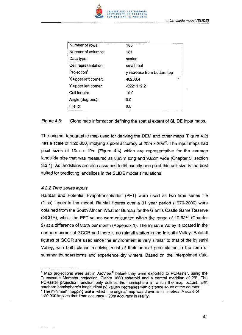
Number of rows:

Number of columns:

Data type:

Cell representation:

Projection1:

X upper left corner:

Y upper left corner:

Cell length:

Angle (degrees):

File id:

185

131

scalar

small real

y increase from bottom top46263.4

-3221172.2

10.0

0.00.0

The original topographic map used for deriving the OEM and other maps (Figure 4.2)

has a scale of 1:20000, implying a pixel accuracy of 20m x 20m2. The input maps had

pixel sizes of 10m x 10m (Figure 4.4) which are representative for the average

landslide size that was measured as 8.93m long and 9.82m wide (Chapter 3, section

3.2.1). As landslides are also assumed to fill exactly one pixel this cell size is the best

suited for predicting landslides in the SLI DE model simulations.

4.2.2 Time series inputs

Rainfall and Potential Evapotranspiration (PET) were used as two time series file

(*.tss) inputs in the model. Rainfall figures over a 31 year period (1970-2000) were

obtained from the South African Weather Bureau for the Giant's Castle Game Reserve

(GCGR), whilst the PET values were calcualted within the range of 10-62% (Chapter

2) at a difference of 8.5% per month (Appendix 1). The Injisuthi Valley is located in the

northern corner of GCGR and there is no rainfall station in the Injisuthi Valley. Rainfall

figures of GCGR are used since the environment is very similar to that of the Injisuthi

Valley; with both places receiving most of their annual precipitation in the form of

summer thunderstorms and experience dry winters. Based on the interpolated data

1 Map projections were set in ArcView® before they were exported to PCRaster, using theTransverse Mercator projection, Clarke 1880 spheroid and a central meridian of 29°. ThePCRaster projection function only defines the hemisphere in which the map occurs, withsouthern hemisphere's longitudinal (y) values decreases with distance south of the equator.2 The minimum mapping unit in which the original map was drawn is millimetres. A scale of1:20 000 implies that 1mm accuracy = 20m accuracy in reality,

from CCWR3 the rainfall values are almost identical and the satistics for rainfall figures

of CCWR3 are therefore considererd representative for the Injisuthi Valley. Rainfall

figures for the Valley ranges between 0.0 to 142.5mm per day for the total of 11 423

days (Figure 2.5).

4.3 PCRaster programming of SLIDE

Mathematical equations for soil moisture fluctuations and resulting changes in slope

stability (section 4.1) were rewritten in PCRaster programming language. Wesseling etal. (1996) provides an elaborate overview of this modeling language. Where

appropriate the calculation units are centimeters (cm), kilo Newton (kN) and days. In

general PCRaster scripts are divided into different sections responsible for different

operations. Basic sections needed for building a sequential model are identified using

the section keywords: binding, areamap, timer, initial, dynamic and report and will be

discussed in the sections below.

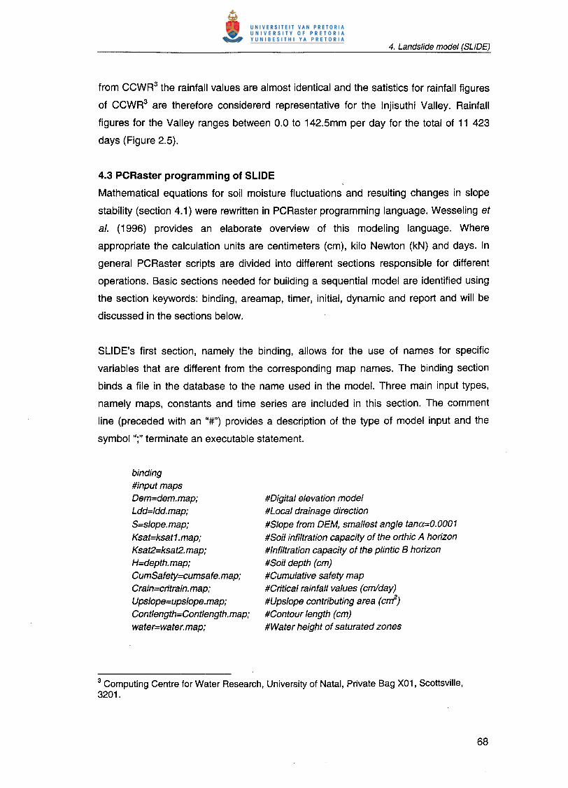
SLIDE's first section, namely the binding, allows for the use of names for specific

variables that are different from the corresponding map names. The binding section

binds a file in the database to the name used in the model. Three main input types,

namely maps, constants and time series are included in this section. The comment

line (preceded with an "#") provides a description of the type of model input and the

symbol ";" terminate an executable statement.

binding#inputmapsOem=dem.map;Ldd=ldd.map;S=slope.map;Ksat=ksat 1.map;Ksat2=ksat2.map;H=depth.map;CumSafety=cumsafe.map;Crain=critrain.map;Upslope=upslope.map;Contlength=Contlength.map;water=water.map;

#Oigital elevation model#Local drainage direction#Slope from OEM, smallest angle tana=O.0001#Soil infiltration capacity of the orthic A horizon#Infiltration capacity of the plintic B horizon#Soil depth (em)#Cumulative safety map#Critical rainfall values (em/day)#Upslope contributing area (eM)#Contour length (em)#Water height of saturated zones

3 Computing Centre for Water Research, University of Natal, Private Bag X01, Scottsville,3201.

#input constantsB=1000;TanPhi=0.554309051 ;Tetamax=0.43;Tetar=0.04;Tetafield=0.10;Cohes=0.00000038;Cohesroots=0.000002;BUlk=O.000 15;Loss=0.1;Gamma Wat=0.00000932;

#monitoring pointsOutFlowPoint=oufflow.map;Out260=out260.map;Out140=out140.map;

#SoillayersFrh1=0.17;Frh2=0.83;

#Pixel size: 10m (1000cm)#Slope angle internal friction#Maximum moisture content (1/100)#Minimum moisture content (1/100)#Soil moisture at field capacity (1/100)#Cohesion (kN/crrt)#Cohesion by grass roots (KN/crrt)#Bulk density (kN/cm3)

#Loss to subsurface geology (em/day)#Unit weight of water (kN/cm3

)

#Oufflow point with soil depth 370cm#Oufflow point with soil depth 260cm#Outf/ow point with soil depth 140cm

#Fraction of orthic A horizon#Fraction of soft plintic B horizon

Areamap, here one map is defined for its location attributes. These location attributes

form the blueprint for all the other input maps in the model that must have similar

location attributes. All the maps generated after running the model are assigned the

attributes of the areamap, in this case the OEM.

areamap

dem.map;

Model calculations are excecuted for 11324 days (31 years) as defined by the rainfall

and PET timeseries files. Iterations can also be set to hours or minutes if required and

if the rainfall and PET data are available at similar scales. Rainfall values for the

Injisuthi Valley were only available per day. There is scope, however, to refine

temporal model predictions by using hourly rainfall data. In the model the timer section

controls the attributes that are responsible for the changes in spatial data over time.

The duration and time slice of the model through three parameters, the start time (day

1), end time (day 11 324) and time slice (1 day).

At the first time step in the model: 1 January 1970, the rainfall does not enter

completely dry soil profile. Instead, it is realistic to expect some intial soil moisture

content as well as an existing soil water height. The initial moisture content was

determined using the volumetric moisture content of the soil in the field during a dry

period, as shown in Equation 4.9 (Morgan et al., 1998).

= volumetric soil moisture content

8m = gravimetric soil moisture content

Ys = dry bulk density of soil (g/m3)

Yw = density of water (0.001 g/m3)

Based on equation 4.9 the initial soil moisture content was calculated as 8v = 1.0 x

0.0001/0.001 = 0.1 for both the orthic A and soft plintic B horizons. The initial value for

water height is estimated at 10cm. In the initial section in the model the initial attribute

values used for the first calculation of the dynamic section, are included as follows:

#initial waterheight

Waterheight =scalar(10);

#initial moisturecontent for day 1 in percentage

Moisturecont1 =scalar(O. 1);

Moisturecont2 =scalar(O. 1);

Overlandflow =scalar(O. 1);

The 'dynamic' section of the model script contains the calculations with all the input

maps written in the sequence in which they occur in the model. It is an iterative section

that is repeated for each time. First, the depths of the unsaturated layers are

determined. Textural differences between the two model layers are distinguished

based on the division between the orthic A and the soft plintic B horizons (Chapter 3,

Sections 3.3.1 and 3.3.3.1), characterized by H1 and H2 respectivley in the model

script. Depth of the unsaturated layers delimits the physical boundaries where water in

the model will move. The quantitly of water that can fluctuate in the soil profile is

determined by the rainfall and potential evapotranspiration (PET) values for the study

area (Chapter 2), as summarised in the timeseries files.

Dynamic

#New depth (cm) of unsaturated layers

H 1 =max(O. 025*H, (H- Waterheight) *Frh 1);

H2 =max(O. 025*H, (H- Waterheight) *Frh2);

#Rainfall and PET in cm per day, both time series files

Precip=timeinputscalar(rain31.tss,clone.map );

PET =timeinputscalar(pet31.tss,clone.map);

PET can only take place when there is more moisture in the soil than the soil moisture

at field capacity (10%). The actual evapotranspiration (AET) is expressed as the actual

evaporation occurring when the soil moisture content is higher than 10%.

The above model statement assumes a linear relationship between AET and rainfall

per day contributing to soil moisture. In reality, however, the AET of water from soil is

constant for a few days after it stopped raining (Ward and Robinson, 1990). After

prolonged dry periods the initial AET would be more than the average percentage PET

calculated in the time series file "pet31.tss' as a result of the dryness of the soil and air

(Ward and Robinson, 1990). Model calculations seem to have abrupt boundaries

determining whether AET will take place. However, working on a scale where the

spatial instability predictions are made per day the AET boundaries are sufficient, as

opposed to predictions that are made per hour or minute where a more precise scale

for PET will be more favorable.

Total moisture that is available for infiltration in the soil profile (Deltamoist1) is

influenced by the amount of precipitation, evaporation and interception (Figure 4.2).

Interception is calculated using the Deltamoist1 values were the AET is already

subtracted from the precipitation. The reason for this is that the natural logarithm (In) in

the PCRaster programming language cannot be applied directly to time series data,

but requires scalar data (Karssenberg, 1994); this results in calculating slightly less

interception. Calculations for include a conversion from cm to mm (section 4.1.5) and

the 'Grass' value is converted from percentage interception to a fraction (1-Grass).

The moisture content minus AET and interception can now enter as the soil profile as

soil water (Figure 4.2).

#Increase (and decrease) in moisture content due to rainfall and evaporation

Deltamoist1 =max(Precip-AET,0.01);

eport dmoist. tss=timeoutput(OutFlowPoint,Deltamoist 1);

#Vegetation interception (Equation 4.8)

Grass=max(O.01 ,(1-((7.6*ln(7175. o*Deltamoist 1))/100)));

Intercept=(Deltamoist1*Grass);

report intercep.tss=timeoutput(OutFlowPoint, Intercept);

#SOIL WATER (Fig 4.2)

Deltamoist=max( (Deltamoist1-lntercept), O.0 1);

#quantity of water entering top soil layer

report atwater. tss=timeoutput(OutFlowPoint, Deltamoist);

If the daily atmospheric water available for infiltration exceeds the infiltration capacity

of the soil (ksat), Horton overland flow will occur (Ward and Robinson, 1990). The

accuthresholdflux operator (Karssenberg, 1994) determines the water flux from the soil

whenever saturated infiltration capacity (Ksat) is exceeded and transports the Horton

overland flow down slope over the local drainage direction map.

Hortonianflow=accuthresholdflux(Ldd, Deltamoist, Ksat);

report horton. tss=timeoutput(OutFlowPoint,Hortonianflow);

When the daily intensity of atmospheric water is less than Ksat, the water will

percolate into the soil. Water percolation in the soils is based on equation 4.4 and the

outflow point defined in Figure 4.2 is used as the point to monitor percolation changes

in both the soil layers.

#Percolation (Equation 4.4)

Bi=(-2. 655)/log 1O(TetafieldIT etamax);

Kteta 1=(Ksat*( (Moisturecont1 )/(Tetamax)) .•.•Bi);

Kteta2=(Ksat2*( (Moisturecont2)/(Tetamax)) .•.•Bi);

Percolation 1=if(Moisturecont1 <Tetafield,O,Kteta 1);

Percolation2=if(Moisturecont2< Tetafield, 0,Kteta2);

report perco 1.tss=timeoutput(OutFlowPoint,Percolation 1);

report per co2. tss=timeoutput(OutFlowPoint,Percolation2);

Water percolating to the subsoil (groundwater in Figure 4.2) results in a decrease in

soil moisture of the upstream pixels and an increase in moisture content for down

stream pixels. Fluctuations in the moisture content falls within the defined minimum

(Tetar=4%) and maximum moisture content (Tetamax=43%) boundaries as measured

in the field and stated in the initial section of the model. Daily changes in the moisture

content for each soil layer at the point of outflow is documented as a time series file.

#Upper soil layer

Moisturecont1 =max(min(Tetamax,Moisturecont1 +(Deltamoist-Percolation 1)/H 1),Tetar);

report moist1. tss=timeoutput(OutFlowPoint,Moisturecont1 );

#Percolating moisture contribution from top soil layer

#Resulting moisture of lower soil layer (slip plane)

Moisturecont2=max(min(Tetamax,Moisturecont2+(Percolation 1-

Percolation2)/H2), Tetar);

report moist2.tss=timeoutput(OutFlowPoint,Moisturecont2);

Water discharged from upstream pixels is based on the local drainage direction of

each pixel and is influenced by the soil depth, slope angle, distance, water height and

infiltration capacity of the soil.

#Water discharge of lower soil layer (Equation 4.6)

#Base flow (Figure 4.2)

Q=Ksat2*S*B*Waterheight;

Inflow and outflow from each pixel results in water height changes. Maximum water

height is determined by the soil depth of each pixel and is a function of the moisture

changes in the soil.

##PORE WATER PRESSURE CHANGE

#Change in water height (pore pressure) of lower soil layer

#First, current water balance (Deltawaterheight)

#Second, inflow from upstream pixels, also lower soil layer

#Third, new water height as a result of inflow and outflow

#Fourth, pore water pressure changes with water height changes

Totalwater=max( ((Waterheight+lnflowdeltawaterheight-Deltawaterheight)

+((Percolation2-Loss)/(Tetamax+0. °1-Moisturecont2))), 0);

report water370. tss=timeoutput(OutFlowPoint, Totalwater);

report water260.tss=timeoutput(Out260, Totalwater);

report water140.tss=timeoutput(Out140, Totalwater);

Waterheight=min(Totalwater, H 1+H2);

report waterh.tss=timeoutput(OutFlowPoint, Waterheight);

report water=Waterheight;

Vertical changes in the water height to a water content higher than the soil depth will

result in saturation excess overland flow. This can be contrasted to Hortonian overland

flow which is a function of the infiltration capacity of the soil being smaller than the

rainfall intensity and the excess of precipitation will flow over the ground surface as

overland flow (Horton, 1933). Saturation excess overland flow is monitored at soil

depths of 3.7m, 2.6m and 104mrespectively. Fluctuations in the water height are also

documented in a time series file (waterh.tss).

#Water height exceeding soil depth is saturation excess overlandflow

#Overlandflow=accuthresholdflux(Ldd, Totalwater,H);

over370=max(if(Totalwater gt 370, Totalwater-370,0),0);

over260=max(if(Totalwater gt 260, Totalwater-260,0),0);

over140=max(if(Totalwater gt 140,Totalwater-140, 0), 0);

#Overlandflow=max(Totalwater-(H1 +H2), 0);

report Land370. tss=timeoutput(OutFlowPoint, over370);

report Land260. tss=timeoutput(Out260,over260);

report Land140. tss=timeoutput(Out140, over140);

Changes in the water height of pixels imply changes in the pore water pressure of the

soil. Changes are the hydrological trigger for slope instability in the Injisuthi Valley

(Chapter 2). In the formula for calculating the pore water pressure changes, the unit

weight of water (GammaWat) is a constant of 9.32kN/m3 (Gardiner and Dackombe,

1983) this was converted to 9.32 x 10-6 kN/cm2 to comply with the model dimensions.

#Changes in pore water pressure.

Porepr =Waterheight*Gamma Wat*sqr( cos( atan(S) ));

The safety factor (F) which is the final calculation expressing probable slope instability

and various factors influencing this ratio, including the changes in pore water pressure

(calculated above), the angle of internal friction of the material (Section 3.3.3.3, Figure

3.8) and the soil cohesion (Section 3.4.5.1). Cohesion is a measure of the average

shear strength and is included in the model as a constant with the value of 3.8x10-7

kN/cm2 (the average measured value). The cohesive effects of grass roots in the area

are added as a constant of 2.0x10-6 kN/cm2 based on the work of Mulder (1991). It is

important to note here that a constant shear strength value gives an indication of the

real cohesion of the soils, and does not allow for the dynamic changes in the cohesion

as a result of the pore water pressure changes in the soils.

report Safety=min(1.5,if(H==0.1, 1.5,((Cohes+Cohesroots)+(H*Bulk*sqr(cos(atan(S)))-

Porepr) *TanPhi) /(H*Bulk*sin( atan(S)) *cos(atan(S)))));

For each pixel the number of days it becomes unstable is recorded in the cumulative

safety map (CumSafety). Where F < 1 a pixel is unstable.

#number of days with safety factor F<1.

report CumSafety =scalar(if(Safety Ie 1,CumSafety+ 1,CumSafety));

The critical rainfall (equation 4.7) for each pixel defines the amount of rainfall needed

to trigger a landslide for a specific pixel. Various PCRcaic operations are summarizedin Figure 4.7.

Digital elevation model(dem.map) .

cel/area. map=scalar(if(dem. mapge 0,1000000,dem.map))

------- -------I

: cellarea.map1- _ _ _ _ _ _ _ _ contiength.map=lookupscalar

(cont.tbl, dem.map)

upslope.map=slopelength

(Idd.map, cel/area.map)

upslope.map=scalar(if(upslope.map Ie 0.01,0.01,upslope.map))

Upslope contributing area(upslope.map)

Contour lengths(contlength.map)

Intermediate maps

Final maps

r - - ---,I ,

t:::J

PCRaster operations for the construction of an up slope contributing

area and contour length map needed for calculating critical rainfall.

At any specific time step, the amount of water in a pixel is dependent on all the

upstream pixels contributing moisture over a local drainage direction. Total up slope

contributing (Figure 4.7) has pixel areas of 1000cm by 1000cm as pixels have sizes of

10m by 10m.

Contour lengths were exported from ArcView 3.1 to Excel and converted to cm with

the altitude categories set at 20m intervals (Appendix 10). The excel file was exported

in ASCII format to PCRaster create a table (contours.tb~ from which a contour length

map was calculated (Figure 4.7). The slope length operation in PCRaster sums the

total amount of pixels that contribute to the downstream pixels based on the local

drainage direction network. All the contributing pixels are assigned the value of the"eel/area. map'.

#Critical rainfall (Equation 4.7)

Crain 1=Ksat*sin(S) *(ContlengthIUpslope) *(Bulk/Gamma Wat) *(1-(SlTanPhi));

Crain2=scalar(if(Crain1 gt 0, Crain+Crain1, Crain));

Crain3=scalar(if(Crain1Ie -2,-2, Crain2));

#rainfall maximum of 20cm is reported.

report Crain=scalar(if(Crain3 ge 20,20,Crain3));

Critical rainfall (Rc) was reported in a map with the defined maximum boundary of

200mm/day and a minimum value of -2mm/day. Although the maximum rainfall for the

period 1970 to 2000 was measured as 142.5mm/day values are documented up to

200 mm/day because these Rc values will not vary as long as the environmental

characteristics are constant. If rainfall data in the future exceed the current maximum

then the probable unstable pixels can still be identified. High Rc values imply stable

pixels and negative Rc values imply pixels where hygroscopic water is present (Borga

et al., 1998).

4.4 Chapter summary

Equations taken from work of Selby (1993), Montgomery and Dietrich (1994) and

Borga et al. (1998) were applied to constructing a hydrological slope stability model

that predict shallow translational landslides in the Injisuthi Valley. Model calculations

have two focuses, namely hydrological changes and mechanical changes in the soil.

Hydrological equations are coupled to the soil mechanical equations through the

fluctuations in water height causing soil pore pressure changes, the main cause of

slope instability.

The SLIDE model was written in PCRaster programming language and a complete

model script is included in Appendix 11. In this script two soil layers are identified in

the model and representing the orthic A and soft plintic B horizons. In each horizon the

hydrological fluctuations are monitored through the creation of time series files and

include daily fluctuations in Horton, saturation excess overland flow, moisture content,

percolation and water height. The time series files will be used to validate the model

performance against field observations, as discussed in the next chapter.

Chapter 5: Model outcome, discussion and predictive power

In this chapter results of the coupled hydrological-slope stability model (called

SLIDE) are presented, discussed and the model is compared to similar existing

models. First, a sensitivity analysis for the constant inputs for SLIDE (Table 3.1) was

conducted after wh~ch the constants are calibrated to optimise model predictions

(Figure 5.1). After optimisation, model instability predictions are compared to the

actual noted landslide positions in the study area. The optimised model is then

applied to an independent northern facing site in the Injisuthi Valley for verification

(Figure 5.1).

Input sensitivityanalysis

Calibration andoptimisation

Landslide predictionmodel

Verification at othersites

The accuracy of the original input topographic map, model calculations and the

fieldwork inputs of the model affect prediction accuracy of SLIDE. Special attention is

given to the accuracy with which the two soil layers are represented by the model, as

the contact between them form the shear plane for landsliding.

SLIDE fundamentally consists of two sub-models, a hydrological model and a soil

mechanical model. The hydrological model is confirmed through the creation of time

series files for soil moisture, percolation and water height fluctuations, as well as

Horton and saturation excess overland flow. The soil mechanical model is confirmed

by comparing the predicted landslides with observed landslide locations. Statistical

expression of model accuracy in terms of correct landslide predictions is based on,

the confusion matrix.

5.1 Statistical analysis of model results

Models that predict the presence or absence of data (Le. landslides) can be judged

by the number of prediction errors, summarised as mainly two types: false positives

and false negatives (Fielding and Bell, 1997). False positives are the pixels predicted

to have landslides when none occurred in reality, while false negatives are the pixels

where landslides are noted in the field but none are predicted by the model (Fielding

and Bell, 1997). By cross tabulating the observed and predicted presence/absence

patterns the performance of a model can be assessed (Fielding and Bell, 1997). This

tabulation is known as a confusion (or error) matrix (Figure 5.2) in which the

categories are presented as pixel counts.

Modelpredictions

+ -+ a b

True positive False positive

- C dFalse negative True negative

Fielding and Bell (1997) describe a variety of measures that can be calculated from a

confusion matrix, and measures applied to the SLIDE model results are summarised

in Tab.le 5.1. Various measures are used as this provides a more thorough test of

model accuracy than would be obtained by purely comparing pixels predicted to be

unstable with those where instability is observed (a true positive test).

Measures of model accuracy based on the confusion matrix classes,

N=a+b+c+d (Figure 5.2) (after Fielding and Bell, 1997).

Measure Definition Calculatio

n1. Sensitivity Ratio of correctly predicted landslides. a/(a+c)

2. Specificity Ration of correctly predicted no landslide d/(b+d)

areas.

3. False positive rate Ratio of wrong landslide predictions. b/(b+d)

4. False negative rate Sites where landslides do occur but where c/(a+c)

not predicted by the model.

5. Correct prediction rate Total correct predictions for landslides and (a+d)/N

no landslide areas.

6. Misclassification rate Wrongly classified landslide and no-landslide (b+c)/N

areas as a ratio of the total area.

Statistics based on the confusion matrix are applied to analysis on the angle of

internal friction (section 5.2.2.2), cumulative safety maps (section 5.3.2) and model

validation (section 5.5) in this chapter and in all the cases the following assumptions

are made:

• Landslides occurring on hillslopes and those occurring in the riverbank slopes are

analysed separately, as river undercutting may trigger landslides.

• Pixel counts on the cumulative safety maps include the inherently unstable pixels

(tan<l»tana) in the classes a and b above, depending on whether they coincide

with observed landslide locations or not. This is done because landslides often

reoccur on old landslide scars on 'inherently unstable' hillslopes.

The model sensitivity analyses, calibrations and optimisations are based on model

runs for the years 1999 and 2000 (731 model iterations), unless otherwise stated.

This time period is selected to save computing time, and also because it coincided

with the fieldwork time of the project. The time selection (1999 and 2000) is further

representative for daily fluctuations between the minimum and maximum rainfall (0-

115mm/day) as the whole modelling time 1970 to 2000, have an annual average of

0-108mm/day with the extreme maximum for the total 31years as 143mm/day. Model

confirmation for the critical rainfall values and total instability days is, however, done

for the total 31 year modelling time, thereby including the maximum rainfall values.

5.2 Sensitivity analysis and calibration of SLIDE

Sensitivity analysis of SLIDE involves measuring the effect of the input parameters

(maps, constants and time series) on the output landslide susceptibility map. For

some of the fieldwork measurements one input constant represents the field-

measured ranges (Le. cohesion and bulk density). Literature estimations for both the

water loss to subsurface geology and the angle of internal friction (</» are te~ted.

Constant model inputs may have a large influence on the model predictions and the

models sensitivity needs to be tested in order to calibrate constants that will optimise

model predictions. Model optimisation and calibration is divided into two sections.

First, the hydrological model and second the mechanical slope stability model.

5.2. 1 Hydrological model

Hydrological fluctuations in the model water height, soil moisture content and

percolation are assessed through the creation of time series files in the SLIDE script

(Chapter 4). Hydrological fluctuations can be assessed by in situ measurements of

water heights if equipment is available (Le. with a tensiometer) (Senarath et al.,

2000), otherwise the hydrological fluctuations can be compared to the original input

quantity of rainfall, as is done in this study. Although this option does not validate the

model against reality, recording fluctuations in soil moisture content can highlight

potential model errors by showing non-monotic behaviour in the time series files.

Further, water entering the soil profile can behave in a predictable manner in a

relative simplistic system such as the SLIDE model. Calibration of some hydrological

parameters may be important to optimise the shallow landslide predictions.

Available water for infiltration in the soil profile ranges between 0-2cm/day for the

years 1999 and 2000 (Figure 5.3). Approximately half of the precipitation is lost to

evapotranspiration and interception before the water enters the soil profile (Figure

5.3) where it can contribute to landslide activity.

- PETRAIN

- VEG-- WATER

Rainfall (RAIN), PET, vegetation interception (VEG) and final

atmospheric water available for infiltration (WATER) during the years

1999 and 2000.

5.2.1.1 Water loss to subsurface geology

Leakage is a factor determined by the porosity of the geology of the area (Figure

4.2), and is practically impossible to measure in the field and therefore usually

estimated (Terlien, 1996) or ignored in landslide models (e.g. Montgomery and

Dietrich, 1994). The effect of water losses can be assessed through time series files

fluctuations in the soil water height. There are no published methods for the

calibration of loss in landslide models and it was therefore decided that water height

fluctuations should resemble seasonal rainfall changes, without excessive build-up or

loss of water during each year.

In Chapter 3 the loss input for SLIDE was set at 0.25 em/day (Terlien, 1996). The

annual average moisture contribution from the atmosphere to the soil is 0.23cm/day

irrespective of season. Based on the known moisture input various different loss

scenarios ranging between 0-1em/day is tested in the model. Zero water loss is

included to access a no-loss scenario and the effect of excessive daily water losses

(1 em/day) included (Figure 5.4).

~ 300EOl~ 200

J> 100

LOSS_O- LOSS_005- LOSS0075- LOSS_01-----. LOSS0125

~ 300EOl~ 200CD

~ 100

i>-;----..'o:.·~-::.~·~""'::C-O~··... ....{/ "............ ...._----------

.~ " .........,;;~~// "

~ LOSS_015- LOSS0175-----. LOSS_025- LOSS_050- LOSS_1

Various water loss scenarios and the influence thereof on the water

height fluctuations, as monitored at the out flow point (Soil depth =370cm).

Losses, exceeding the average daily moisture contribution of rainfall (O.23cm/day),

namely the original SLIDE input: 0.2S em/day (LOSS_02S) and also O.SOcm/day

(LOSS_OSO)and 1 em/day (LOSS_1), all result in dry soil profiles over time (lower

Figure S.4). Evidently these losses are too high to be realistic for the study area.

A zero loss scenario (LOSS_O)on the other hand, results in sudden peaks of water

height increases up to 4S0cm (Figure S.4). Inserting minor water loss in SLIDE

prevents this sudden unnatural concentration of water in the soil, as is evident from

the losses of O.OSem/day (LOSS_OOS),0.07Scm/day (LOSS_007S) and a loss of 0.1

em/day (LOSS_01) (Figure S.4). Of these minor losses, the curve of water height

fluctuations with a loss of 0.1em/day most clearly resembles seasonal fluctuations in

the water height (Figure S.4) and this value will replace the original loss of 0.2S

em/day in the model.

5.2.1.2 Moisture content and percolation

To confirm the texturally different behaviour of the two soil layers in SLIDE, namely

the orthic A and soft plintic B horizons of the Westleigh soil form, fluctuations in the

soil moisture and water percolation are compared (Figure 5.5).

~ 0.14

1~ 0.10'

M1

2001 - M2

Moisture content and percolation fluctuations in the orthic A (M1 and

P1) and soft plintic B (M2 and P2) horizons of a 370 cm deep soil with

a water loss of 0.1 cm/day to the subsurface geology.

Figure 5.5 clearly shows the larger fluctuations in the moisture of the orthic A horizon

compared to the lower soft plintic B horizon. This modelling is realistic as water

percolation is influenced by the infiltration capacities of the soils. Higher infiltration

capacity for the upper orthic A horizon results in a higher soil moisture content, with

larger quantities of water available for percolation, compared to the lower plintic B

horizon. Apart from differences in infiltration capacity the soft plintic B horizon

contains more clay than the upper soils (Chapter 3), and the water retention ability is

higher resulting in less water percolation. Increased clay content of lower soil layer is

also responsible for a higher average moisture content, seldom falling below the soil

moisture at field capacity (0.10) although the model script leaves scope to fall to

minimum moisture boundary (0.04) as can be observed in the top soil layer. In

general moisture content fluctuations (Figure 5.5) fall within the boundaries of the

field measurements where the minimum is 4%, field capacity 10% and the maximumof 43% soil moisture.

Soil moisture and percolation differences in the model are realistic for the two

different soil layers with regard to soil moisture and water percolation. In practice

water will percolate through the top soil layer, having a higher infiltration capacity, but

concentrate at the infterlace between the orthic A and the more clay rich soft plintic B

horison. Local pore water pressure within this region of the soil rises, resulting in

potential instability at the shear plane between the two soil horisons. This observed

phenomena is accurately modelled with SLIDE.

5.2.1.3 Horton and saturation excess overland flow

In the orthic A soil horizon, Horton overland flow occurs when rainfall intensity

exceeds the infiltration capacity. It is expected that no Horton overland flow will

occur, as the maximum rainfall intensity 143cm/day for 1970-2000 and the minimum

infiltration capacity of the orthic A horizon is 158cm/day. Model output for Horton

overland flow confirmed this expectation with Oem/dayfor all 31 years. High rainfall

intensities frequently occur for the duration of a few minutes that will result in Horton

overland flow, which implies that a finer temporal modelling scale (Le. daily or hourly

predictions) will result in Horton overland flow.

When soil water heights in the orthic A and soft plintic B horizons increase to exceed

the total soil depth, saturation excess overland flow (SAT) occurs. Using a water loss

of 0.1em/day in the model, fluctuations of SAT is monitored at the three different

control points with soil depths of 370cm, 260cm and 140cm respectively (Chapter 4).

Fluctuations in the water height (w in Figure 5.6) and SAT (0 in Figure 5.6) are

presented in Figure 5.6.

Evident from Figure 5.6 is that SAT is likely to occur in shallower soils (0140 AND

0260) as no SAT is noted at a soil depth of 370cm. SAT is defined as the total soil

water minus the total soil depth. Not only does soil depth, but also position on the

landscape influence the amount of saturation excess overland flow that will occur

(Le. pixels with a larger upstream contributing are area will have larger quantities of

overland flow).

i~Gmmmm:mmmmmmm:mmmmmm:m:1 - W3703: -50 ~~~~--~~~~. ~~. ~~~~~~~~~. '-'-'1999 2000 2001 - 0370

Water height fluctuations (w) and saturation excess overland flow (0)

for monitoring points with soil depths of 140cm, 260cm and 370cm

respectively.

5.2.2 Mechanical slope stability model constants

Three model constants describing soil properties, namely bulk density, cohesion and

angle of internal friction are assessed for model sensitivity. This is done by

comparing the cumulative instability maps, as defined in the infinite slope equation

for instability (Equation 3.3), the method described by Borga et al. (1998).

5.2.2.1 Bulk density and cohesion

Bulk density and cohesion are model constants based on the arithmetic mean of field

measurements. The minimum, mean and maximum of the field-measured ranges

(Table 5.2) are substituted in the model and the cumulative instability maps

compared.

Bulk density and cohesion ranges as tested in the cumulative safety

map covariance correlation (in model units: kN/cm3).

Minimum Mean MaximumBulk density kN/cm;jx 10·;j 0.05 0.10 0.15Cohesion kN/cm~x 10.0 0.21 0.38 0.56

Differences in the eventual cumulative safety map are analyzed using a map

covariance correlation in the Grid Analyst extension in ArcView 3.1®. The control map

(Table 5.3) had mean values for both the bulk density and cohesion as listed in Table

5.2. The other four maps have the minimum or maximum of bulk density and

cohesion respectively. Map comparisons for cumulative safeties are done over a 31-

year period (1970-2000) and the spatial covariance matrices (Table 5.2) for the

cumulative instability maps showed a correlation between 99.84% and 100%.

Covariance correlation matrix for cumulative safety maps with a range

of cohesion and bulk density values.

Control Cohesmin Cohesmax Bulkmin Bulkmax

Control 1.00 1.00 1.00 0.9988 0.9998

Cohesmin 1.00 1.00 1.00 0.9988 0.9998

Cohesmax 1.00 1.00 1.00 0.9988 0.9998

Bulkmin 0.9988 0.9988 0.9988 1.00 0.9984

Bulkmax 0.9998 0.9998 0.9998 0.9984 1.00

Changes in cohesion do not at all influence model predictions, whilst changes in bulk

density cause minor changes in the model landslide susceptibility map (Table 5.3).

Using average bulk density values in SLIDE, results in safety maps that are 99.88%

similar to maps where the minimum bulk density values are used and 99.98% similar

to when maximum bulk density values are used. From Table 5.3 it is evident that all

the maps are all very similar to each other, and it can be concluded that SLIDE is not

sensitive to the measured ranges for bulk density and cohesion. It is further safe to

assume that cohesion and bulk density can be represented by the arithmetic mean of

the field-measured ranges in the SLIDE model.

An additional factor for increased cohesion as a result of reinforcement of grass roots

(O.000002kN/cm2, Chapter 4) is added in the model. This cohesion factor plus the

mean cohesion is in the vicinity of the maximum tested cohesion, and it will not affect

the instability predictions. Yet, it makes the model more realistic and is therefore

added.

5.2.2.2 Angle of internal friction

Angle of internal friction (<1»is a constant of 31° used in the SLIDE model (Section

3.3.3.3), based on the range of 28°-34° proposed Gardiner and Dackombep983) for

sandy soils. Literature examples of threshold angels, are extremely varied and

include angles of 6°-14° for soils form weathered clays and shales in semi-frictional

conditions with the possibility of high water-tables; 19°-28° for semi-frictional sandy

soils in upland England and Wyoming, 21°_42° in the Ardennes, and 33°-55° for

frictional soils in Colorado and California (Van Asch, 1983; Selby, 1993). In order to

calibrate and optimise the model with respect to <1>,various values starting at: <1>=10

followed by various intervals of <1>ranging between 14° to 44° for each model run

(1999-2000) are used. The effect of variations in <1>are determined by comparing pixel

counts on the cumulative landslide susceptibility maps.

Counts of the confusion matrix categories are obtained using the Grid Analyst

extension and extracting the x,y,z values for each model run in ArcView 3.1®. Details

of the counts are summarised in Appendix 12. Counts are used in different measures

to express model accuracy that are based on the confusion matrix (Table 5.3).

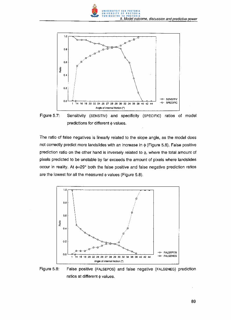
Figure 5.7 summarises the rate of correctly predicted landslides (sensitivity) and

correctly predicted non-landslide areas (specificity) for different <1>values. Evident

from Figure 5.7 is that sensitivity and specificity is equally high at <1>=29°.Sensitivity

increases at lower <1>values as a result of all the slopes being predicted unstable and

thereby including all the possible landslide predictions. Specificity behaves as the

inverse of sensitivity and increases with higher <1>where fewer areas correctly

predicted to have no landslides.

1.0

0.8

0.6

.2(;jcr

0.4

0.2

--<>- SENSITIV-0- SPECIFIC1 14 16 18 20 22 24 26 27 28 29 30 32 34 36 38 40 42 44

Angle of internal friction (0)

Sensitivity (SENSITIV) and specificity (SPECIFIC) ratios of model

predictions for different <1> values.

The ratio of false negatives is linearly related to the slope angle, as the model does

not correctly predict more landslides with an increase in <1> (Figure 5.8). False positive

prediction ratio on the other hand is inversely related to <1>, where the total amount of

pixels predicted to be unstable by far exceeds the amount of pixels where landslides

occur in reality. At <1>=29° both the false positive and false negative prediction ratios

are the lowest for all the measured <1> values (Figure 5.8).

1.0

0.8

0.6

a.~cr

0.4

0.2

0.0

....0

.....p.

O'.Q....O···

0 ...-0....0 ...0 ..--<>- FALSEPOS-0- FALSENEG1 14 16 18 20 22 24 26 27 28 29 30 32 34 36 38 40 42 44

Angle of internal friction (0)

False positive (FALSEPOS) and false negative (FALSENEG) prediction

ratios at different <1> values.

Correct classification ratio peaks at high <I>values whilst the misclassifications are

high at low <I>values (Figure 5.9). At an angle of internal friction lower than 14°

(Figure 5.9) the correct and misclassifications ratios are both 50%. At a <1>=29°the

misclassification rate is 0.16 and the correct classification rate is 0.84.

1.0

0.8

0.6

°~a:0.4

0.2

0.0

D.."0.

"0 .

.'0.."0 ..'0·..0....0....0

.

0 ....0....0

.

·0....

1 14 16 18 20 22 24 26 27 28 29 30 32 34 36 38 40 42 44

Angle of internal friction (0)

-0- CORRECT--0- MISCLASS

Correct (CORRECT) and misclassification (MISCLASS) ratios at different

<I>values.

According to Figure 5.9 the model correct classification rate for <1»40°is 1 and the

misclassification rate is 0, a seemingly perfect prediction ratio. These ratios, however

should be treated with caution, as high <I>values (larger than 40°) only include the

landslides occurring on slopes in the region of 40° angles. The statistical behaviour

of both the curves in Figure 5.9 can be explained by the relative differences in pixels

counts for classes in the confusion matrix, where a possible 37 pixels represent

correct landslides predictions versus a total of 6111 possible pixels representing the

rest of the study area. Further, the correct no-landslide locations has also large pixel

counts (6111-37) and this resulting invariably in very high and very low ratios for high

angles of internal friction, and inversely for low <I>values. Large differences in pixel

counts dominate the correct and misclassification ratios and these ratios should

therefore be applied with caution for very high or low <I>values.

An alternative approach to evaluate the accuracy of model predictions is presented

by multiplying the ratio of correct no landslide predictions by the number of correctly

predicted landslides, as follows: [(diN) x a/(a+c)]. This ratio includes three categories

of the confusion matrix as well as the total number of pixels. In Figure 5.10 it is

evident that model predictions, based on this ratio, peak at <1>=29°.

0.8

0.7

0.6

°.~ 0.5c:

~ 0.4"Cl'!Q.

U 0.3~0(..)

0.2

0.1

1 14 16 18 20 22 24 26 27 28 29 30 32 34 36 38 40 42 44

Angle of internal friction (')

Figure 5.10: Ratio of correctly predicted no-landslide and landslide pixels for

different <1>values.

In order to optimise model predictions, the range of input values for the angle of

internal friction of soils (<1» are tested. Model predictions, measured in terms of the

false positive and false negative prediction ratios, sensitivity and specificity all

confirm optimum model predictions at <1>=29°. This <1>value falls within the literature

suggested values for sandstone soils ranging between <1>=28° to 34° (Gardiner and

Dackombe, 1983). Since the ratio of correctly predicted landslides and no landslides

areas also indicate optimum model predictions at <1>=29° this value is used in the

model, replacing the previously used arithmetic mean of the literature suggested

range (<1>=31°).

In this section of model calibration and optimization, two model constants have been

adjusted. In the hydrological section of the model a loss of water to subsurface

geology is added to give realistic fluctuations in the hydrology of the study area, and

in the soil mechanical section the angle of internal friction of the soils are changes to

optimise model predictions at <1>=290•Based on Figure 5.1 the optimized model are

used run and predicted instability zones compared to actual landslide zones,

described in the next section.

5.3 Model confirmation

Model confirmation again focuses on the two sections of the model separately.

Critical rainfall figures are used to assess the hydrological section of the model and

the cumulative instability map is used to assess combined effects of hydrology and

mechanical slope stability.

5.3.1 Critical rainfall

Critical rainfall (Rc) of a pixel is the static amount of water needed to cause instability

under existing topographic conditions. It is calculated independently of the available

rainfall in a specific environment (equation 4.7), and is therefore an ideal way of

confirming predicted Rc values with realistic rainfall figures of the area. It is expected

that high Rc values correlate with unconditionally stable pixels, whilst low Rc values

for pixels indicate unstable pixels. Figure 5.11 is the critical rainfall value map

calculated for SLIDE. Observed landslide locations are overlayed with the Rc map

and occur in areas where no rainfall is needed to trigger landslides, in other words

inherently unstable areas (Figure 5.11). Critical rainfall (Rc) areas above 5cm/day are

the flatter areas in the study site while Rc values above 15cm/day are never

predicted unstable in the study area for the 31 year modelling time (Figure 5.11).

Based on Figure 5.11 the Rc value classes for all the landslide pixels (divided into

hillslopes and riverbank slope landslides) as opposed to the percentage noted for the

whole study area is summarised in Table 5.4. Landslides occurring on hillslopes

mostly contain Rc values for hygroscopic water and imply that no water is needed to

trigger landslides (Table 5.4). Eight percent (3 of 37 pixels) of the hillslope landslides

require rainfall figures between 0-143cm/day to cause instability, this is within the

rainfall boundaries for the modelling time 1970-2000. Only four landslide pixels (11%)

fall outside the modelling time boundaries, and will not be predicted unstable.

Of the landslides occurring in river banks, 36% could possibly occur during the

modelling time, and 64% were stable pixels that required more rainfall to be triggered

than actually occurred during 1970-2000 (Table 5.4). In the total study area 83% of

the pixels (n=6111) were predicted as being inherently unstable and 81% (n=37) of

the observed landslides occur within this predicted area (Table 5.4). This shows a

strong correction between the actual and predicted location of landslides based on

Rc values. The mean Rc value for 95% of the pixels representing the study area fall

within 10.9 ±9.0cm/day.

Legend

c:=:J study area boundaryRivers

• Landslides

Cirtieal rainfall (em/day)c:=:J <0c:=:J 0c::::::::J 1-5~ 5-10_ 10-15_ 15-20

In SLIDE Rc was calculated using the equation form Borga et al. (1998) with

principles of the quasi-dynamic wetness index (Barling et al., 1994). Borga et al.

(1998) also used Rc to define potential zones of instability. The quasi-dynamic

wetness index and Rc as calculated in SLIDE allow for an increase in the up-slope

contributing area for cells placed downstream of bedrock outcrops. The model also

allows for the incorporation of storms having varying intensity-duration-frequency-

characteristics. The Rc values predicted to induce slope instability may not readily

apply to actual rainfall values necessary to trigger landsliding but provide a relative

index of the potential for shallow landsliding (Montgomery et al., 1998). Pixels of

equal Rc values can be interpreted to have similar environmental controls on shallow

landslide initiation.

Catchment and observed landslide percentage areas in each critical

rainfall range.

% Observed landslide areas % Predicted Rc ofCritical rainfall (Rc)

Hillslopes Riverbank Study area

Hygroscopic water <Oem/day81 0 83

(Unconditionally unstable)

Rainfall 0-14.3cm/day 8 36 3

Rainfall 14.3-20cm/day11 64 14

(Unconditionally stable)

The Rc values calculated in the model reflect a single static figure and do not give an

indication of the changes in Rc with different rainfall intensities. In reality, Rc values

are dynamic e.g. a low intensity of rainfall over a three-day period can raise regolith

moisture content above a critical level for stability, whilst high rainfall over a longer

period allows pore water pressure to dissipate before it becomes critical (Borga et al.,

1998). The high rainfall intensities over a short period may result in more runoff and

less infiltration, and thereby not influence instability. Garland and Oliver (1993) noted

a tendency for events with large numbers of landslides occurs towards the end of the

wet season reflects the seasonal build-up of regolith moisture content in creating

suitable mass movement conditions, and could be the reason for King's (1982)

earlier "two event hypothesis". Water from the first event needs time to soak the

weathered overburden thoroughly before the second rainstorm can trigger a failure.

The critical rainfall value is complex and dependent on the local conditions. Campbell

(1975) noted that landslides might be expected on days where the rainfall exceeds

235mm. Can uti et al. (1985) observed that precipitation in excess of 10mm over a 1

to 3 day period caused landslides in marly arenaceous rocks. An important

theoretical premise of the critical rainfall value is that both the antecedent soil water

and event water have an important contribution towards shallow landsliding (Crozier,

1999). For example, Pasuto and Silvano (1998) found that the peak rainfall at 24-48

hours preceding the onset of movements is important. Accumulated rainfall also sets

conditions for shallow failure as shown by Garland and Oliver (1993). Antecedent

water in the Injisuthi Valley is accounted for in SLIDE through soil water height

fluctuations that increase during times of increased rainfall and sets the conditions for

shallow landslides that are then triggered by varying amounts of 'event' water.

5.3.2 Classification of the safety factor

The cumulative instability map contains four safety factor classes, summarised in

Table 5.5, based on definitions of Montgomery and Dietrich (1994). From Table 5.5 it

is evident that discrepancies between the stable and unconditionally stable classes

are not effective for SLIDE as the unconditionally stable pixels (tana < 0.938.tanlj»

with tan29°=0.554, and stable pixels (Table 5.5) are merged in this model as tanlj>is

multiplied with a factor of 0.938 and this does not leave much scope for pixels to be

included in the stable class. The stable and unconditionally stable classes are

actually one class.

Pixel counts for the classification of the safety factor based on the

cumulative safety map.

Safety factor Definition Pixel count

1. Unconditionally unstable tana>tanq, 972

2. Unstable Predicted to fail according to Equation 138

3.3.

3. Stable Insufficient drainage area to fail. 0

4. Unconditionally stable tana < tanq,(1-(y.Jy)) 5001

Total pixels 6111

Unconditionally instable pixels (Table 5.5) imply slopes with an exposed soft plintic B

horizon. From Table 5.5 138 pixels (16%) are predicted to fail according to the safety

factor equation; of these only four pixels are not included in the unconditionally

unstable class. The four pixels not included above correlate with the four pixels of

which the critical rainfall values are larger than the observed rainfall figures for the 31

year modelling time. Unconditionally stable classes overlap to the extent that they

comprise one class that includes 82% of the study area. Unstable pixels formed 2%

of the study area of site are predicted to be unconditionally unstable. 73% of the

observed landslides coincide with unconditionally unstable areas. Montgomery and

Dietrich (1994) and Borga et al. (1998) who observed more than 80% of the

predicted landslides to be unconditionally unstable or to fail with low rainfall.

Unconditionally unstable pixels as identified by the cumulative safety map, correlate

with the critical rainfall maps and clearly shows the trend that shallow landslides

often occur on top of old landslide scars. The model predicts this phenomenon

correctly as is observed in the field.

Some of the inherently unstable pixels occur on slopes with gradients steeper than

50° and soil depths of 0.1cm (Chapter 3). In general slope angles in the study area

vary between 0.1°-70.9° with an average slope of 17.6°. Ninety five percent of the

slopes in the study fall within slopes of 17.6°±13.4°, containing enough soil for

shallow landslides.

Figure 5.12 shows the model predicted landslide locations as overlaid by observed

landslides. The mean predicted unstable days over 31 years is 1652 days. The

model does not predict landslides occurring in the riverbank slopes, as the scale of

topography is too small to show topographical changes as a result of river incision,

such as steep riverbanks. SLIDE is also written with assumptions and equations

(Chapter 3) for rainfall triggered landslides, and not for river undercutting triggers

resulting in shallow landslides. The model can be more accurate with larger scale

topographic maps. Another factor influencing accuracy is the pixels sizes used for

the maps. Shallow landslides, however, occurring on slopes are successfully

predicted by the model (Figure 5.12).

The SLIDE model frequently predicts shallow landslides to occur on inherently

unstable slopes (tana,>tan<1».The inherently unstable slopes consist of exposed

plintic B horizon, or old landslide scars. On top of the scars shallow recurring

landslides are predicted by the model as it has been noted in the field. Conditions

resulting in instability in the recent past are still active on the slopes. Old landslide

scars may also be the collecting places for water and the heads of the drainage

network. Faces of spurs may be at frictional angles and hollows containing fine-

grained soil may have high pore-water pressures and are probably close to semi-

frictional angles, a state of inherent instability.

Legend

C=:J Study areaRivers

Landslidesoland'" river

Total unstable daysC=:J 0C=:J 1 - 100C=:J 100 - 200lWAI 200 - 500_ 500-1000_ 1000-5000_ 5000 - 11324

According to Van Asch (1983), inherently unstable slopes predicted by the model are

not constantly in a process of mass movement but may contain a phase during which

the regoliths are in a state of temporary stability. Slope angles may have reached a

certain threshold value, which depends on the strength characteristics of the regolith

and the possibility to build up positive pore-water pressure within it (Van Asch, 1983).

When the conditions of strength and pore-water pressure in the regolith change, the

regolith becomes unstable and mass movement will occur until a lower threshold

angle of the slope is achieved (Van Asch, 1983). Phases of stability may alternate

with phases of instability due to changes in the strength of the regolith by weathering

processes or climatological changes (Van Asch, 1983). The slopes in the study area

are, therefore, characterised by a succession of stable (threshold slopes) and

unstable phases, not always predicted by the model, but confirm field observations.

Generalisation and uncertainty of original input data (soil depth, moisture content,

soil strength, bulk density etc.) to calculate the stability of the slope is expressed as a

safety factor. According to Selby (1993) this safety factor can not been seen as

absolute stability value of a slope as there is a non-linear relationship between the

safety factor and the danger of sliding (Selby, 1993). This implies that the distinction

between inherently unstable pixels and stable pixels may be clear in theory. In

practise the total amount of days that a pixel is unstable does not render it more

unstable, as there is not linear relationship. It is therefore also acceptable for

observed landslide locations to overlap with pixels that are inherently unstable.

5.4 Model accuracy

Accuracy of SLIDE will be discussed the next section and include aspects of the pixel

size and local drainage direction.

5.4. 1 Pixel size

Topographic map used in the SLIDE analysis is captured at a scale of 1:20000. The

effect of scale on the accuracy of model predictions is assessed by applying SLIDE

to two sets of identical models the one using maps with pixels sizes of 20m x 20m

and the other with maps of 10m x 10m pixels. SLIDE was originally constructed using

pixels sizes of 10m by 10m as these most closely represent the average landslide

sizes (as noted in Chapter 3). Differences in the cumulative safety maps for the years

1999-2000 are presented in Figure 5.13.

In the 20m x 20m cumulative safety map, 12 landslides out of the possible 37 are

correctly predicted (Figure 5.13 (A)). This compared to the 31 out of 37 correctly

predicted landslides using 10m pixel maps, is very low (Figure 5.14(8)). The 10m-

pixel map predicts larger unstable areas and more landslides fall within unstable

regions. At first sight the 20m pixel map (A) seems as if the unstable predicted areas

include the landslide locations but with the actual landslide locations overlay it is not

clearly visible that these areas fall outside the landslide locations.

Statistics based on the confusion matrix (Figure 5.2) indicate the influence of pixels

size on the prediction accuracy. Pixels sizes of 10m x 10m result have high

sensitivity and specificity ratios and relatively low ratio of wrongly predicted landslide

or no-landslide areas (false positive and false negative rates) when compared to the

20m x 20m pixel maps.

Nw-tELegend

• Landslides

s Rivers

c=J Stable pixels

300 0 300 Meters ~ Unstable pixels

Figure 5.13: SLIDE cumulative safety maps for model iterations using pixel sizes of

(A) 20m x 20m and (8) 10m x 10m.

Table 5.6: Model accuracy as influenced by map pixel size.

Map pixel size

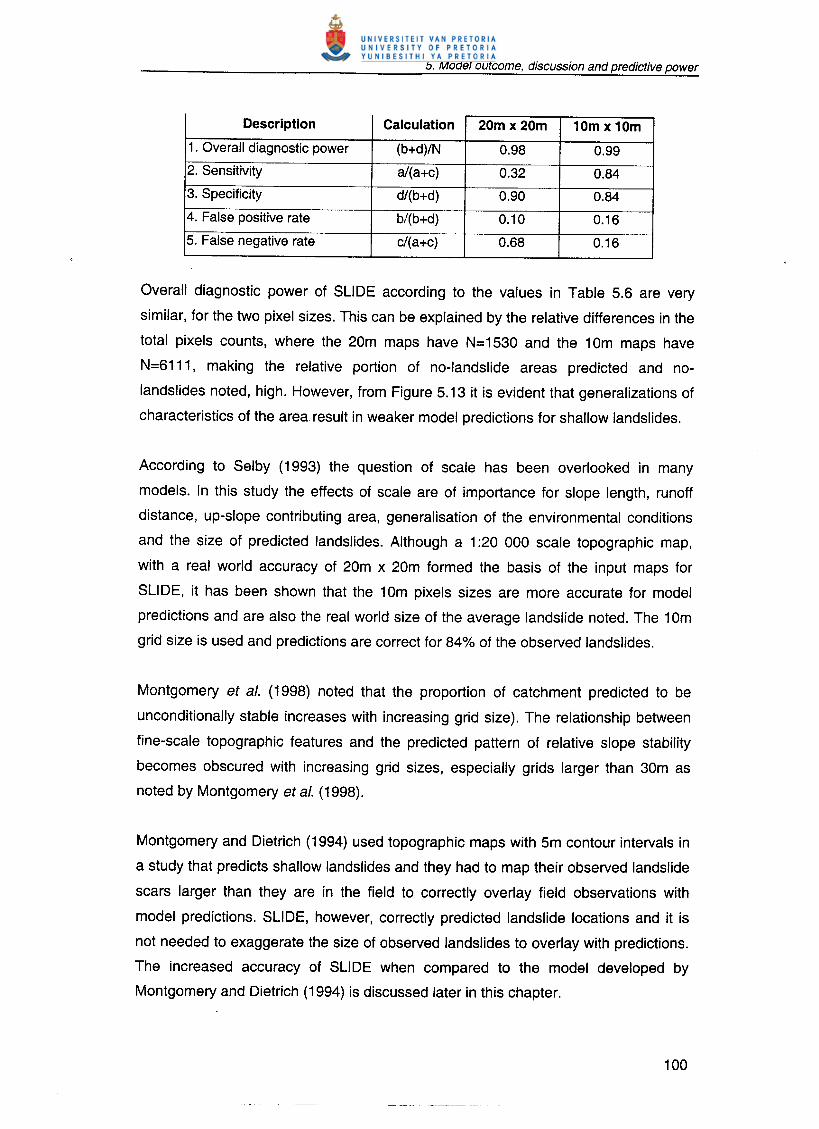
Description Calculation 20m x 20m 10m x 10m

1. Overall diagnostic power (b+d)/N 0.98 0.99

2. Sensitivity a/(a+c) 0.32 0.84

3. Specificity d/(b+d) 0.90 0.84

4. False positive rate b/(b+d) 0.10 0.16

5. False negative rate c/(a+c) 0.68 0.16

Overall diagnostic power of SLIDE according to the values in Table 5.6 are very

similar, for the two pixel sizes. This can be explained by the relative differences in the

total pixels counts, where the 20m maps have N=1530 and the 10m maps have

N=6111, making the relative portion of no-landslide areas predicted and no-

landslides noted, high. However, from Figure 5.13 it is evident that generalizations of

characteristics of the area result in weaker model predictions for shallow landslides.

According to Selby (1993) the question of scale has been overlooked in many

models. In this study the effects of scale are of importance for slope length, runoff

distance, up-slope contributing area, generalisation of the environmental conditions

and the size of predicted landslides. Although a 1:20 000 scale topographic map,

with a real world accuracy of 20m x 20m formed the basis of the input maps for

SLIDE, it has been shown that the 10m pixels sizes are more accurate for model

predictions and are also the real world size of the average landslide noted. The 10m

grid size is used and predictions are correct for 84% of the observed landslides.

Montgomery et al. (1998) noted that the proportion of catchment predicted to be

unconditionally stable increases with increasing grid size). The relationship between

fine-scale topographic features and the predicted pattern of relative slope stability

becomes obscured with increasing grid sizes, especially grids larger than 30m as

noted by Montgomery et al. (1998).

Montgomery and Dietrich (1994) used topographic maps with 5m contour intervals in

a study that predicts shallow landslides and they had to map their observed landslide

scars larger than they are in the field to correctly overlay field observations with

model predictions. SLIDE, however, correctly predicted landslide locations and it is

not needed to exaggerate the size of observed landslides to overlay with predictions.

The increased accuracy of SLIDE when compared to the model developed by

Montgomery and Dietrich (1994) is discussed later in this chapter.

Montgomery et at. (1998) also noted that OEM's do not always adequately represent

relevant topographic attributes (eg. fine-scale hollows, channel slope and channel

confinement, further, mountain drainage basins are characterised by temporal

variably in landscape characteristics that arise from disturbance and recoveryprocesses.

5.4.2 Loca/ drainage direction (LOO)

Flow paths of ground water are presented in a LDD map, where a drainage direction

is assigned to one pixel. The LDD successfully represented water flow in the study

area to be predominantly downward (to the north) and identifies areas of water

concentration.

A more sophisticated LDD map with multiple flow directions for one pixel is described

by Borga et at. (1998) within the modules of WOOITEM (Watershed Oriented Digital

TErrain Model). Where cumulative flow at a point should be distributed among more

than one neighbouring down-slope pixel, multiple flow directions are assigned to

pixels (Borga et a/., 1998). The concept of multiple down slope flow represents the

convergence or divergence of flow under the control of topographic curvature, more

accurate than the modules in PCRaster does. However, at the scale of modelling

SLIDE is constructed, the uni-directional LDD accurately presented the landscape.

5.5 Vegetation recovery and landslide age

As indicated in Figure 3.11, most of th~ landslides in the study area are noted to

have 60% or more vegetation recovery, and only a small number of the slides show

no vegetation recovery. It is assumed in the model that landslides showing more

vegetation recovery are older scars than those with no recovery. This is not always

realistic as slides on very steep slope sections may take a longer time for grass

seeds to disperse and grow within the scars. However, SLIDE predicts most of the

landslides to occur on inherently unstable slopes, which in reality they have

significant grass recovery. Older landslides can therefore occur on inherently

unstable slopes, as it has been frequently observed that almost fully recovered

landslides have smaller secondary sliding within the original scar. The older

landslides do, therefore, occur on inherently unstable slopes. Refinement of the

temporal predictions of the model can be done in combination with the vegetation

recovery rate, as described by Guariguata (1990), Myster et al. (1997), Myster and

Walker (1997) and Robertson and Augspurger (1999).

5.6 Model verification

A north facing site directly west of the study area (Figure 5.14) is selected to validate

SLIDE. All the field measured and literature model input parameters derived for study

area S were applied to the validation area (V in Figure 5.14). A new set of maps were

constructed based on the topography of area V (scale 1:20 000) which result in a

unique LDD and slope angles (Figure 4.3). Although the validation area is

independent of the original fieldwork done in area S, the geology, soil and vegetation

properties on northern facing sites in the Little Berg are homogenous (Chapter 2). As

a result of the validation area being independent of the model calibrations based on

prediction accuracy of study area S, the application of the model to area V forms a

test for model predictive power for northern facing slopes in the Injisuthi Valley in

general.

Evident from Figure 5.14 is that steeper sections in the validation area (V) are

predicted to be unstable in the same manner as for the study area (S). For the study

area (S) 31 of the 37 landslides (84%) are correctly predicted in comparison with the

validation area (V) where 36 of the 44 landslides (82%) are correctly predicted to

occur within unstable predicted zones. It is evident that SLIDE predictions for both

the sites are high and this also illustrates that the study area selected for fieldwork

(Chapter 3) is representative with regards to geology, soils and vegetation for

northern facing sites in the Injisuthi Valley, located in the Little Berg (Chapter 2). The

results support that SLIDE can be applied to other northern facing areas in the Little

Berg, KZN Drakensberg and it will yield a high correct landslide prediction ration

using the inputs provided (Chapter 3).

...~ .N."~P!

S

Legend

Total unstable daysc==J 0c==J 1 - 100~ 100-500_ 500-1000_ 1000-5000_ 5000 - 11324

ContoursRivers(S) Study area boundary(V) Validation area boundaryLandslides

Landslide susceptibility map and observed landslide positions

for the validation (V) and study area (S).

5.7 Comparison to other existing hydrological-slope stability models

Various shallow landslide models have been based on the infinite slope equation

combined with hydrology. Some major differences and improvements, which SLIDE

offers, are briefly outlined using two similar published models (Table 5.7). O'Loughlin

(1986) developed TOPOG a model that uses a steady state rainfall and maps of

spatial pattern of equilibrium soil saturation based on the analysis of up-slope

contributing area to predict shallow landslides. Montgomery and Dietrich (1994)

applied TOPOG to a 1.2km2 basin in California and a O.3km2 drainage basin in

Oregon. The second model for comparison is WODITEM (Watershed Oriented

Digital TErrain Model) applied to a 5 km2 catchment in northern Italy (Borga et a/.,

1998). The primary assumptions and equations of SLIDE, TOPOG and WODITEM

are similar with differences outlined in Table 5.7.

SLIDE TOPOG WODITEMDEM scale 1: 20 000 1: 4800 1: 10000Grid sizes used 10m 5m 10mStudy area 3km£ 1.2 km£and 0.3 km£ 5km£Landslide GPS fieldwork Aerial photograph Field identificationidentification recognitionFieldwork derived • Bulkdensity x • Bulkdensityinputs • Soilthickness • Soilthickness

• Saturatedinfiltrationcapacity

• CohesionLiterature derived • Angleof internal • Angleof internal • Angleof internalinputs friction friction friction

• Vegetation • Saturated • Saturatedcohesion infiltrationcapacity infiltrationcapacity

• Vegetation • Cohesion • Cohesioninterception • Bulkdensity

• SoilthicknessRainfall data Real-life data Steady state amounts Steady state amountsSoil horizons Two texturally Assume spatially Assume spatially

different layers uniform layer uniform layerHorton overland flow 1/ x XSaturation excess 1/ Xoverland flow x

Critical rainfall 1/ .,I .,I

Although TOPOG uses 5m contour intervals for the model predictions they are not as

accurate as the predictions of SLIDE. This could be a result of the literature derived

inputs for TOPOG that are too general to sufficiently represent the study areas (Table

5.7). SLIDE, on the other hand, uses field measurements and literature derivations

based on fieldwork (Le. angle of internal friction based on texture analysis) for model

inputs. This results in higher representability of the study site and increases model

predictive power. In the TOPOG model the position of existing landslides were

determined using aerial photograph observations (see Chapter 3 for a critique on

these techniques) as opposed to GPS positioning of landslides for SLIDE

confirmation (Table 5.7). Consequently the known landslide locations of TOPOG had

to be exaggerated to fall within the predicted instability zones, while the position of

landslides in SLIDE were accurate within the 10m by 10m scale.

WODITEM and TOPOG both assume a spatially uniform soil layers while two

texturally different soil horizons are accurately modelled in SLIDE with the contact

between the two layers acting as the shear plane for landslides. Scripts for Horton or

saturation excess overland flow are included in SLIDE, which are ignored in

WODITEM and TOPOG (Table 5.7). The models TOPOG and WODITEM offer

limited scope for effective temporal predictions if they are not based on observed

rainfall quantities but static state rainfall values (Table 5.7). Realistic rainfall values

are used in SLIDE for the northern facing Injisuthi Valley and offer scope forexpanding temporal predictions.

5.8 Chapter summary

Calibration and optimization of the components of water loss to subsurface geology

in the model are set to 0.1 cm/day and the soil angle of internal friction is set to

<1>=29°.Map covariance correlation matrixes of the cumulative landslide susceptibility

maps showed that SLIDE is not sensitive to the field measured ranges for bulk

density and cohesion and that the mean of these ranges can successfully represent

the ranges as constants in SLIDE. The differences in the orthic A and soft plintic B

horizon were successfully represented by differences in the moisture content and

water percolation fluctuations predicted by the model.

The effect of pixel size on the accuracy of model predictions revealed that 10m pixels

resulted in more accurate landslide predictions as opposed to 20m pixel maps. At

10m the landscape is more defined and landslide predictions closer to the real world

size of shallow landslides as noted in the study area (Chapter 3). Cumulative

susceptibility maps (with 10m pixels) successfully predict 31 of the 37 observed

landslides occurring in the slope in the study area Sand 36 of the 44 landslides in

the validation area.

Landslides noted in the river bank soil are not predicted by the model and this is a

result of the map scale not showing changes in topography where rivers incise.

Consequently the steep slopes of riverbanks are not inserted in SLIDE. Landslides in

riverbanks are further frequently triggered by river incision as opposed to slope

landslides that are triggered by rainfall. SLIDE predictions takes into account both the

slope angle and rainfall intensity of each pixel when calculating instability. This

explains why no landslides occurring in the riverbanks are predicted by SLIDE.

Critical rainfall values for each map pixel confirmed cumulative instability maps for

shallow landslides on slopes. Most of the correctly predicted landslides occur on

inherently unstable slopes requiring no rainfall to slide. This phenomenon is

observed in the field as new landslides recurring at old landslide scar locations, Le.

on inherently unstable slopes.

Chapter 6: Conclusion

In this study a coupled rdrOIOgiC-SIOpestability model (called SLIDE) for theprediction of shallow, rainfal -triggered translational landslides on the northern slopes

of the Injisuthi Valley was de eloped. SLIDE assesses the relative potential for shallow

landslide initiation in steep, soil-mantled terrain underlain by sandstone geology, with

soil and vegetation properties typical for slopes of the Little Berg (Chapter 2) in the

KZN Drakensberg.

Landform in the model was represented by a digital elevation model (OEM). Various

field measurements based on the approach by Mulder (1991), Montgomery and

Dietrich (1994) and Borga et a/. (1998) included soil saturated infiltration capacity, soil

depth, soil texture, bulk density, cohesion and vegetation type was taken. All the

environmental parameters contributed to the timing, size and behaviour of shallow

landslides in the Injisuthi Valley. Field measurements, local drainage direction maps

and rainfall figures for the area proVided constraints in hydrologic behaviour of the

landslide prediction model (SLIDE) based on daily rainfall data for 31 years (1970-

2000).

By using equations for shallow landslide assessment (Montgomery and Dietrich, 1994

and Borga et a/., 1998) two main sections namely a hydrological section and a slope

mechanical section were identified. Equations defining both sections were written in

PCRaster dynamic modelling language, a GIS package. Hydrological fluctuations in

the model were monitored through the creation of time series files. Time series files for

soil moisture and percolation revealed different hydrological behaviour of the orthic A

and more clay rich soft plintic B horizons of the Westleigh soil type. The orthic A

horizon had a higher infiltration capacity, and consequently higher moisture andpercolation fluctuations compared to the soft plintic B horizon. This hydrological

difference results in water concentration at the interface between the texturally

different soil horizons and a local increase in pore water pressure at the interface

between the two soil layers and forms the shear plane for landsliding. In the upper soil

layer (orhtic A) the model script accommodated Horton overland flow when rainfall

intensity exceeded the saturated infiltration capacity of the soil. Saturation excess

overland flow occurred in shallow soils after increases in water height exceeded the

total height of the orthic A plus soft plintic B horizons.

Model sensitivity analysis for parameters that were inserted in the model as constants

showed that the model was not sensitive for the field measured ranges of bulk density

and shear strength. The mean of these ranges can be used to represent the soils in

the model. Optimisation of model predictions through calibrating for water loss to

subsurface geology simulated seasonal fluctuations in soil water height. The angle of

internal friction for the soils was calibrated to 29° based on the prediction accuracy of

the model.

Prediction accuracy of the model was assessed using a confusion matrix where four

pixel categories were identified, namely landslides and no-landslide areas for the two

classes of observed and predicted pixels. Various statistics based on the relationship

between these classes were used to express model accuracy. In the study area,

where model inputs were measured 84% (31 of 37) of the observed landslides were

correctly predicted, after model calibration and optimisation. To validate ttie model it

was applied to an independent north facing slope in the Injisuthi Valley where 82% (36

of 44) of the observed landslides were correctly predicted. This confirms that the

litohological, soil and vegetation properties of the Little Berg (lower than 2000m a.s.l.)

which were similar throughout the northern facing Injisuthi Valley.

SLIDE landslide susceptibility maps predicted that shallow landslides were generally

concentrated on slopes ranging between 15°-45° in the Injisuthi Valley. Evidently, the

local surface topography was one of the dominant controls in landsliding, defining the

local slope, soil thickness and shallow subsurface flow convergence. Landslides

occurred within an optimum slope range of 15°-45° where the soils are deep enough to

cause sliding and the gravitational force contributes significantly to the shear stress.

The SLIDE susceptibility maps successfully delineated areas on the landscape with

similar topographic control on shallow landslide initiation, as was observed in the field.

Critical rainfall values (Rc) for each pixel gave an indication of the amount of water

needed under prevailing topographic and environmental conditions to cause instability.

Rc values were correlated with safety factor values, and unstable areas had low Rc

values, which indicated possible instability. Although the Rc value was one static value

the antecedent water in the Injisuthi Valley was accounted for in SLIDE through soil

water height fluctuations. Water height fluctuations increased during times of

increased rainfall and set the conditions for shallow landslides, which were then

triggered by varying amounts of 'event' water. Event water (Rc) calculated in SLIDE

confirmed landslide susceptibility calculations, as predicted instability zones had lowRc values.

Several advantages of SLIDE over existing hydrological-slope stability models include

the simulation of two texturally different soil layers (orthic A and soft plintic B) where

differences in soil moisture and percolation fluctuations are critical for defining the

shear plane for sliding. Further, scripts for Horton and saturation excess overland

flows are included in SLIDE, as it is realistic to assume that not all the atmospheric

water contributes to soil water and eventually landsliding. The GPS positioning of

observed landslides proved an accurate way to confirm landslide locations compared

to aerial photo identification and field mapping used in other landslide models. As a

result of all the above-mentioned factors the prediction accuracy SLIDE was higher

than similar existing models.

Although the prediction accuracy of SLIDE is high (>80%) there is scope for

improvement. SLIDE ignores the hydrological complication caused by the presence of

natural soil pipes and possibly other macropores carrying significant downslope flows

that were observed in some parts in the study area. Soil pipes act as bypasses to soil

flow and additionally the speed delivery to the slope base of whatever inflow received.

The presence of soil pipes connected with the surface posed serious limitations to the

representativenes of the hydrological model. However, owing to difficulties and

uncertainties in pipeflow modelling, according to Borga et al. (1998) it is a likely

component to remain and intratable part of the hydrological model. The influence of

soil pipes may, however, be assessed by applying SLIDE and monitoring of landslide

dynamics in the areas present and adjacent to soil pipes.

SLIDE can further be extended to include rotational landslides, of which there were 13

noted in the study area. Rotational slides are based on other equations and

assumptions than translational landslides, of which 85 where noted in the study area.

This would also add to the understanding of the contemporary landscape of the

Injistuhi Valley. The current translational landslide susceptibility analysis was based on

topography as depicted by a OEM. Extrapolations of SLIDE for predicting future

landslide susceptibility zones could be based on patterns of landslides that reflect the

current fire and land management regimes (Bijker et al., 2001). Additionally patterns of

high intensity rainfall that can localise shallow landsliding in mountainous terrain

(Montgomery et al., 1998). Within this context a simple physically based model of the

topographic control (SLIDE) on the potential for shallow landslide initiation can provide

spatially explicit hypotheses against which to interpret observed pattern of slope

instability. Additionally improving temporal predictions using fine scale rainfall data

may extend SLIDE using topographical maps with 5m contour intervals to define

riverbank incisions in the landscape. Steep slopes should be identified at the

riverbanks and the local drainage direction network of the area resulting in water

concentrations in certain areas and increasing probability for instability. Expression of

the cumulative susceptibility map as probabilities and not as total days may also be an

option to consider for future modelling. A variety of technical developments (Le

improved OEM interpolation and LDD derivation) will in future lift the constraints that

currently bind the accuracy of any physical based landslide model in a GIS.

Development of expertise on shallow landslide modelling in South Africa will also

improve the knowledge and rigorous experimental procedures of applying theory to

models.

From a research perspective, SLIDE is the first known attempt to develop an

integrated model for shallow landslide prediction in South Africa. Natural processes

operating on a slope to cause shallow landslides are successfully represented by themodel. SLIDE is a tool that can be used by the KwaZulu-Natal Wildlife for field

management and selecting sites for development such as roads or hiking trails and in

the Little Berg. Areas susceptible for potential shallow landsliding are delineated, while

the application to land use decisions still requires evaluation and requires jUdgement

of values external to the model framework, Le. additional weight of road, or number of

hikers on a slope etc. For naturally triggered landslides, however, the delineation of

unstable areas is accurate for north-facing sites in the Injisuthi Valley. The equations

used to construct SLIDE, are based on physical relationships between hydrology and

slope instability and can therefore be easily applied to other areas experiencing

shallow landslides in South Africa, with re-measurement of the model inputs. SLIDE

can be applied in its present condition to other areas in South Africa and also forms a

stepping stone for further development of geomorphological modelling of our

subcontinent.